Constraining biospheric carbon dioxide fluxes by combined top-down and bottom-up approaches

While the growth rate of atmospheric CO₂ mole fractions can be measured with high accuracy, there are still large uncertainties in its attribution to specific regions and diverse anthropogenic and natural sources and sinks. A major source of uncertainty is the net flux of carbon dioxide from the biosphere to the atmosphere, the net ecosystem exchange (NEE). There are two major approaches to quantifying NEE: top-down approaches that typically use atmospheric inversions and bottom-up estimates that rely on process-based or data-driven models or inventories. Both top-down and bottom-up approaches have known strengths and limitations. Atmospheric inversions (e.g., those used in global carbon budgets) produce estimates of NEE that are consistent with the atmospheric CO₂ growth rate at regional and global scales but are highly uncertain at smaller scales. Bottom-up data-driven models based on eddy-covariance measurements (e.g., FLUXCOM) match local observations of NEE and their spatial variability but have difficulty in accurately upscaling to a reliable global estimate.

In this study, we propose combining the two approaches to produce global NEE estimates, with the goal of capitalizing on each approach's strengths and mitigating their limitations. We do this by constraining the data-driven FLUXCOM model with regional estimates of NEE derived from an ensemble of atmospheric inversions from the Global Carbon Budget 2021. To do this, we need to overcome a series of scientific and technical challenges when combining information about diverse physical variables, which are influenced by different processes at different spatial and temporal scales. We design a modeling structure that optimizes NEE by considering both the model's performance at the in situ level, based on eddy-covariance measurements, and at the level of large regions, based on atmospheric inversion estimates of NEE and their uncertainty. This resulting “dual-constraint” data-driven flux model improves on information based on single constraints (either top down or bottom up), producing robust locally resolved and globally consistent NEE spatio-temporal fields.

Compared to reference estimates of the global land sink from the literature, e.g., Global Carbon Budgets, our double-constraint inferred global NEE shows a considerably smaller bias in global and tropical NEE compared to the underlying bottom-up data-driven model estimates (i.e., single constraint). The mean seasonality of our double-constraint inferred global NEE is also more consistent with the Global Carbon Budget and atmospheric inversions. At the same time, our model allows for more robustly spatially resolved NEE. The improved performance of the double-constraint model across spatial and temporal scales demonstrates the potential for adding a top-down constraint to a bottom-up data-driven flux model.

1 Introduction

The annual growth of carbon dioxide in the atmosphere has been directly measured with high accuracy since 1957 (Keeling et al., 1989). However, attributing changes in atmospheric CO₂ to regional fluxes and to the respective anthropogenic and natural sources and sinks is prone to uncertainties. One of the main sources of uncertainty is the land biosphere, which has large uncertainties both in the human-related and the natural flux components (Friedlingstein et al., 2022). Improved understanding of processes driving variations in the global carbon cycle requires, among other things, improved observational constraints on the net flux of carbon dioxide from the land surface to the atmosphere or net ecosystem exchange (NEE) across local, regional, and global scales (Bastos et al., 2022; Ciais et al., 2022; Gaubert et al., 2019; Saeki and Patra, 2017; Thompson et al., 2016).

Two different approaches to constrain sources and sinks of carbon dioxide can be distinguished: top-down and bottom-up estimates (Crisp et al., 2022; Friedlingstein et al., 2022). Top-down approaches typically correspond to atmospheric inversions, which infer the surface fluxes over land and ocean based on observations of atmospheric CO₂ mole fractions based on a Bayesian inversion framework using prior estimates of the flux of carbon dioxide and an atmospheric transport model (Chevallier et al., 2005; Peylin et al., 2013; Crisp et al., 2022; Ciais et al., 2022). Bottom-up approaches typically rely on in situ observations and/or remote-sensing data combined with statistical upscaling techniques or process-based terrestrial biosphere and land surface models to infer local to regional or global NEE (Jung et al., 2020; Kondo et al., 2020)

The strengths and limitations of each approach are largely inherited from the “point of view” of the system. Top-down approaches, using regional and global observations and mesoscale to global-scale atmospheric transport, view the integral of fluxes from large areas. They produce reliable estimates of the magnitude and variability of latitudinal distribution of NEE, finding solutions that are in line with the global atmospheric growth rate (Gaubert et al., 2019; Friedlingstein et al., 2022). However, this aggregated view can compromise the local estimates of NEE, as the system adjusts sub-regional NEE to match the overall target, with estimates becoming increasingly uncertain for smaller regions (Ciais et al., 2010). Inverse models are rarely evaluated at the scale of individual ecosystem sites as the mismatch in spatial scales represented is simply too large.

Bottom-up approaches include a diversity of measurements, from small-scale direct observations at the leaf, plant, plot, and ecosystem scale to remote-sensing observations of relevant proxies (e.g., biomass, greenness) (Friedlingstein et al., 2022; Jung et al., 2020; Kondo et al., 2020). These approaches are sensitive to small-scale heterogeneity in the land surface and can provide information on the local distribution and magnitude of NEE. The FLUXCOM project (Jung et al., 2020) produced a comprehensive comparison of data-driven bottom-up approaches for upscaling terrestrial biosphere carbon dioxide and water fluxes based on eddy-covariance measurements. The FLUXCOM ensemble produced consistent spatial patterns of global NEE compared with process-based models (Jung et al., 2020), indicating that the model ensemble captured the relevant ecosystem-level processes. However, data-driven ecosystem-level flux models, including FLUXCOM, have a strong bias for NEE in the tropics compared to top-down estimates (Kondo et al., 2015; Jung et al., 2020), given that they depend on unevenly distributed eddy-covariance observations, which are particularly sparse in the tropics (Tramontana et al., 2016; Chu et al., 2017). Furthermore, micrometeorological conditions under the canopy in tropical forests can lead to data collection problems at tropical towers due to low nighttime turbulence (Hayek et al., 2018; Fu et al., 2018; Jung et al., 2020) creating an incorrect learned relationship between driver variables and NEE. These two limitations result in global estimates of NEE that are far from other best estimates of NEE (Jung et al., 2020).

Previous studies have suggested that observations of atmospheric CO₂ could provide an additional constraint to bottom-up data-driven flux models (Jung et al., 2020; Anav et al., 2015). However, given the mismatch in spatial scales, processes, and uncertainties between the two approaches (Ciais et al., 2022), even reconciling such estimates constitutes a challenge (Deng et al., 2022; Friedlingstein et al., 2022; Crisp et al., 2022; Ciais et al., 2022; Bastos et al., 2022). The two approaches also produce a different view of the flux, sensitive to different scales and processes of the land surface, such as fire and inland waters (Ciais et al., 2022). Thus, it is not trivial to constrain a bottom-up data-driven flux model with a top-down view of atmospheric CO₂. Here, we aim to test the hypothesis, proposed in these previous studies, that a bottom-up data-driven flux model trained with a complementary constraint based on top-down atmospheric inversions can improve the estimates of regional and global land surface CO₂ fluxes. To do this, we first create a data-driven flux model analogue to a FLUXCOM member (Jung et al., 2020) trained on the observed NEE from eddy-covariance sites. Then, in parallel, we test the effect of adding an additional top-down constraint to the model's objective function used in NEE optimization. This top-down constraint is based on the regional integrals of NEE from an ensemble of atmospheric inversions. The addition of a top-down constraint to the bottom-up model requires solving a number of technical challenges to realistically link the two very different types of reference datasets in the objective function used to optimize NEE. We then evaluate the ability of the double-constrained model to estimate global and regional NEE, its spatial variability, and its temporal variability from seasonal to inter-annual timescales.

2 Data

2.1 Net ecosystem exchange

The carbon fluxes included in estimates from top-down and bottom-up approaches are not exactly the same, as described in detail in Ciais et al. (2022). The primary observational constraint of top-down methods is atmospheric CO₂ observations, which are sensitive to nearly all carbon exchanges between the atmosphere and land ecosystems, as well as fluxes from inland water systems (lakes, rivers). In contrast, eddy-covariance flux measurements reflect carbon exchange across a smaller footprint of typically a few hundred meters, and their location is often selected to explicitly exclude the influence of fires and inland water systems. A meaningful comparison between fluxes derived from each thus requires adjusting for both fires and inland water fluxes, as also discussed in Friedlingstein et al. (2022), Ciais et al. (2022), and Deng et al. (2022). In this study, we account for these inherent differences as described in Sect. 2.3. From hereon, we refer to “NEE” as land carbon exchanges excluding inland water systems and fire fluxes.

2.2 Eddy-covariance site-level data

This study uses the same in situ data as used in the FLUXCOM system in Jung et al. (2020) and Tramontana et al. (2016) (see the supplement from Tramontana et al., 2016 for a full list of included sites). The data-driven flux models are trained using meteorological observations and NEE data collected by globally distributed eddy-covariance towers in the La Thuile synthesis dataset of the and CarboAfrica network (Valentini et al., 2014) FLUXNET network (https://fluxnet.fluxdata.org/data/la-thuile-dataset/, last access: 15 May 2022). Following Tramontana et al. (2016), driver variables are created using a set of remotely sensed and meteorological data from the Moderate Resolution Imaging Spectroradiometer (MODIS) data (http://daac.ornl.gov/MODIS/, last access: 15 May 2022) and the European Center for Medium-Range Weather Forecasting ERA5 atmospheric reanalysis dataset (https://www.ecmwf.int/en/forecasts/dataset/ecmwf-reanalysis-v5, last access: 15 May 2022) (Table A2). At tower locations, the meteorological data are derived from the FLUXNET towers using ERA5 data for gap-filling following Tramontana et al. (2016), while the global dataset uses only ERA5 data. See Tramontana et al. (2016) for a full discussion of the handling of meteorological data. Furthermore, the FLUXCOM-RS+METEO V1 NEE ensemble data using ERA5 meteorological forcing from Jung et al. (2020) were used to generate the regional sparse linear models described below.

2.3 Atmospheric inversions

Atmospheric inversions use observed CO₂ mole fraction from in situ measurement stations and flask network, or satellite retrievals of total column CO₂ (XCO₂), with estimates of the non-biogenic fluxes to infer the exchange of carbon between the land, oceans, and atmosphere. The land–atmosphere fluxes from atmosphere inversions correspond better to net biome productivity, or the total regional gain or loss of carbon from all processes, i.e., including the signal from fires and other disturbances, land use change and management, and river evasion (Ciais et al., 2022).

Chevallier et al. (2005)van der Laan-Luijkx et al. (2017)Rödenbeck et al. (2003, 2018)Feng et al. (2016)Palmer et al. (2019)Niwa et al. (2022)

Table 1 Atmospheric inversions from the Global Climate Project 2022 (Friedlingstein et al., 2022), respective period covered, and original references.

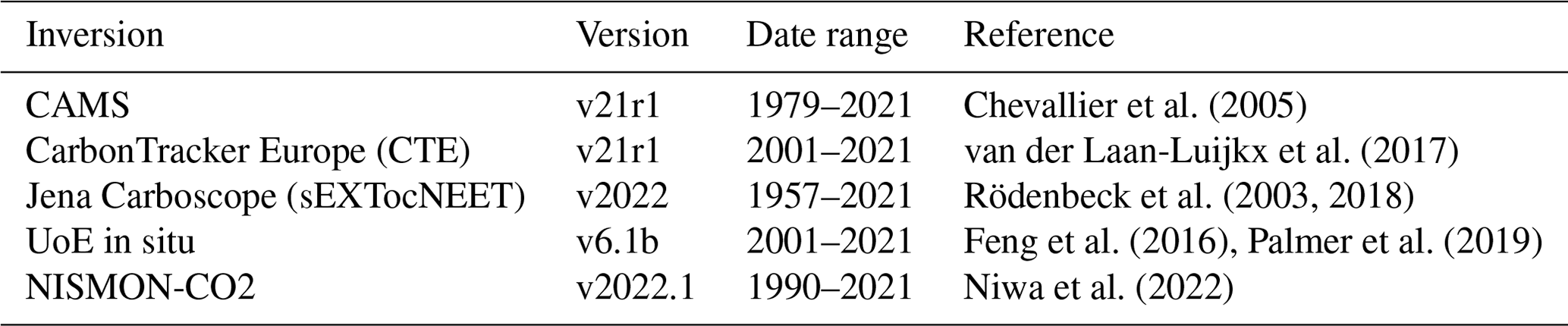
For the top-down constraint (referred to as “atmospheric”), we use the estimates of the land–atmosphere exchange from five models from the ensemble of atmospheric inversions from the Global Climate Budget (Friedlingstein et al., 2022, GCB2022) as described in Table 1. See Friedlingstein et al. (2022) for a full discussion of inversion systems. Only atmospheric inversions based on surface observations are used since they cover the study period used here, i.e., 2001–2017 (Table 1). All inversion results were provided on a common 1° × 1° lat–long grid and monthly temporal resolution.

The inversion estimates as provided by Friedlingstein et al. (2022) have been adjusted to rectify small differences in prescribed fossil fuel emissions, cement production, carbonation fluxes, and lateral riverine CO₂ transport. We further subtracted fire emissions for each individual inversions at grid cell level. For the fire emission adjustment, we used the gridded fire fluxes from CAMS Global Fire Assimilation System (GFAS) (Di Giuseppe et al., 2018) without additional adjustment, which is consistent with the CarbonTracker Europe treatment of fire. The resulting fluxes thus represent land ecosystem carbon exchange excluding inland waters and fires, comparable with NEE estimates based on upscale of eddy-covariance measurements.

While pixel-level NEE estimated by atmospheric inversions are known to be under-constrained (Ciais et al., 2010; Kaminski and Heimann, 2001) and are unlikely to provide robust constraints of NEE to train our model, atmospheric inversions produce reliable estimates of the magnitude and variability of latitudinal distribution of NEE, finding solutions that are in line with the global atmospheric growth rate (Gaubert et al., 2019). Therefore, we aggregate the NEE from the inversions by a set of 18 very large regions consistent with the regions in the Regional Carbon Cycle Assessment and Processes-2 (RECCAP2) project (Tian et al., 2018). This aggregation leverages the growing consensus about the magnitude of global NEE from atmospheric inversions (Gaubert et al., 2019) allowing for a “global” constraint from a set of smaller regional constraints which cover the land surface.

Note that the ensemble of inversions used here is not the source of the land sink estimate of the GCB2022, which is calculated as the residual land sink derived from other major independent terms in the global carbon budget (emissions from fossil fuels and industry (E_FF) + emissions from land use change (E_LUC) − the ocean sink (S_ocean) − atmospheric growth rate (G_ATM)), and used here as reference for the global evaluation of our NEE estimates.

3 Methods

This study is based on two models, illustrated in Fig. 1: a bottom-up data-driven model that upscales NEE from eddy-covariance measurements using a neural network with remote-sensing and meteorological predictors (hereafter referred to as the EC model) and a single objective function (training term 1 in Fig. 1), similar to the FLUXCOM model (Jung et al., 2019), and a model that uses the same neural network structure but uses a dual-objective function, which includes training term 1 (as in the EC model) and a second training term (training term 2) based on top-down regional constraint based on atmospheric inversions (hereafter referred to as the EC-ATM model). The optimization of NEE by EC-ATM is challenged by the spatial, temporal, and physical units mismatch between the two training terms: training term 1 is based on daily in situ NEE from eddy covariance (in g C m⁻² d⁻¹) and training term 2 is based on monthly NEE integrated over very large regions from atmospheric inversions (in Pg C per month). In order to link effectively across scales in the training of EC-ATM, we connect the neural network with a pre-computed statistical model that acts as a “bridge” between site-level NEE and regional integrals, allowing the neural network to learn efficiently from both bottom-up and top-down data streams.

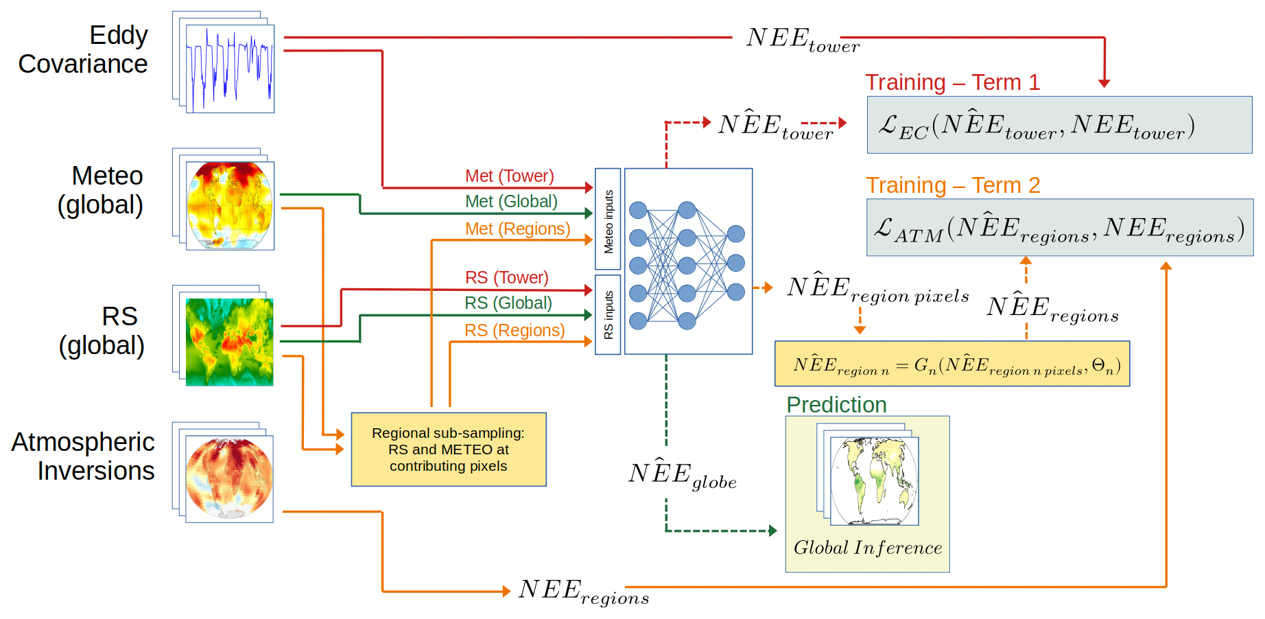
Figure 1 The EC model considers only the first term of the objective function (red lines). The EC-ATM model consists of the bottom-up data-driven flux model (red lines) plus an additional constraint derived from atmospheric inversions (orange lines). In the first training pass, the neural network takes meteorological observations from eddy-covariance towers, along with remotely sensed (RS) data to create an inference of NEE, which is compared with the observed NEE in the first term of the objective function. In the second training pass, the neural network takes meteorological and RS variables at pre-selected pixels for each region. The inferred NEE at these pixels is fed into the regional bridge models to create inferences of regional NEE, which are compared with the regional integrals from an ensemble of atmospheric inversions. For global inference the neural network takes global meteorological data from ERA5 along with RS data to estimate NEE for all land pixels (green lines).

In this section, we first present a description of the predictors used for NEE upscale (referred to as driver data (Sect. 3.1), then a description of the single- and double-constraint EC and EC-ATM models (Sect. 3.2 and 3.3), including the statistical approach proposed to bridge across scales in EC-ATM (Sect. 3.3), then we discuss the training approach for each model (Sect. 3.4) and finally the post hoc analysis performed (Sect. 3.5).

3.1 Model driver data

We use the driver variables from the FLUXCOM-RS+METEO with ERA5 forcing ensemble as in Jung et al. (2020), i.e., enhanced vegetation index (EVI), fraction of absorbed photosynthetically active radiation (fAPAR), daytime land surface temperature (LST_day), nighttime land surface temperature (LST_night), the medium infrared reflectance band (MIR), Normalized Difference Vegetation Index (NDVI), Normalized Difference Water Index (NDWI), extracted for each site and globally from MODIS, and the ERA5 variables of incoming global radiation (R_g), top-of-atmosphere potential radiation (R_pot), water availability index (WAI), and air temperature (T_air). The full set of drivers were constructed following Jung et al. (2020) and Tramontana et al. (2016); see Appendix Table A2 for the driver formulation. These variables are computed globally and stored by plant functional type (PFT) derived from the MODIS Land Cover Type yearly L3 global 500 m dataset collection 5 (Friedl et al., 2010) and are reconstructed here by the percentage of the component PFTs in each pixel following the approach in Jung et al. (2019) and Tramontana et al. (2016). Two drivers, WAI and T_air, are used at daily time step, while the other eight are constructed from the mean seasonal cycle (MSC) signal across the component variables. All are used at a 0.5° spatial resolution.

3.2 EC model description

The bottom-up data-driven flux model takes as input observations of meteorological and remotely sensed drivers at a location, available from either eddy-covariance towers or satellite platforms, and outputs an inference of the NEE for that location. This bottom-up model consists of a feed-forward neural network or a set of fully connected network layers, which we train using the standard gradient-based backpropagation algorithm (Kelley, 1960). The fully connected layers consist of nodes or “neurons”, which are exposed to the output of all neurons in the previous layer. Nonlinearity is introduced by passing each node output through a nonlinear activation function. Our network is a set of three fully connected layers with the Rectified Linear Unit (ReLU) activation function (Agarap, 2019). We provide a detailed illustration of the model architecture in Appendix Fig. B1.

The bottom-up model (EC model) is trained using an objective function with one term which compares the model's inference of NEE and the observed NEE at the eddy-covariance site. The EC model is run and trained only on data from eddy-covariance towers and co-located pixels. The EC model is identical to an ensemble member of the FLUXCOM system (Jung et al., 2020; Tramontana et al., 2016). For each experimental run we train the EC model independently (Fig. 1, red lines), to provide a paired test of the impact of the additional atmospheric constraint.

3.3 EC-ATM model description

To improve regional and global upscaling performance, this study builds a second model (EC-ATM model), starting with the same bottom-up model, to which we add a second term to the objective function comparing the NEE output, inferred at regional scale using the regional models, with the integrals of regional NEE from an ensemble of atmospheric inversions (Fig. 1, orange lines). To rule out effects of parameter initialization, we use the same initial state for the EC and EC-ATM neural networks.

Statistical bridge models

When calculating the atmospheric term of the objective function, running the bottom-up model for every land pixel and fully calculating the global integral of NEE is too computationally intensive to train a data-driven model in a reasonable time frame. This study solves this problem by using pre-computed statistical models to calculate fast approximations of the regional integral based on a limited number of pixels for each region. We build this set of bridge models from the FLUXCOM RS+METEO NEE results (Jung et al., 2020) by finding stable linear relationships between the NEE at fixed spatial locations within the region with the regional integral of NEE in the same time period.

The bridge models are created using least absolute shrinkage and selection operator (Lasso) regression. Lasso regression extends ordinary least squares (OLS) regression by adding a term to the objective function (Eq. 1) where N is the number of observations, P is the number of independent variables, and y is the dependent variable. This term is a weighted ℓ₁ norm, or the mean of the absolute values of the parameters of the linear model β, times the weighting term α. This additional term has the effect of driving some weights to zero as α is increased (Tibshirani, 1996).

$$\begin{array}{}\text{(1)}& \mathrm{Minimize}:\sum _{i=\mathrm{1}}^N{\left(y_i-\sum _{j=\mathrm{1}}^P{x}_{ij}{\mathit{\beta }}_j\right)}^{\mathrm{2}}+\mathit{\alpha }\sum _{j=\mathrm{1}}^P\left|{\mathit{\beta }}_j\right|\end{array}$$

The dependent variable for the Lasso regression is the regional integral of the monthly ensemble mean NEE derived from the global NEE data from the FLUXCOM intercomparison, specifically the RS+METEO setup (Jung et al., 2020). The regional integrals are calculated as the sum of NEE for all non-zero pixels p∈P_t in the region for time steps t in all times T (Eq. 2). The independent variables are the per-pixel monthly mean values of NEE, p∈P_t, for time step t. Using this formulation, the spatial logic of the regression is to find a stable set of weights relating the NEE at geographic locations within the region to the regional integral of NEE. This logic is then extended using Lasso regression (Eq. 3), where the reduction of weights in the model to zero creates a sparse solution. This can be interpreted as discovering a subset of geographic locations whose NEE values are minimally sufficient to produce a high-quality estimate of the regional NEE from the FLUXCOM RS+METEO results. This quality is quantified as the R² value of the NEE inferred by the sparse Lasso model regressed against the regional integrals of NEE. The FLUXCOM RS+METEO data are thereafter only used for model evaluation.

$$\begin{array}{}\text{(2)}& {\displaystyle }{\mathrm{NEE}}_t=\sum _{p=\mathrm{0}}^P{\mathrm{NEE}}_{tp}\text{(3)}& {\displaystyle }\mathrm{Minimize}:\sum _{t=\mathrm{0}}^T{\left({\mathrm{NEE}}_t-\sum _{p=\mathrm{0}}^{P_s}{\mathrm{NEE}}_{tp}{\mathit{\beta }}_p\right)}^{\mathrm{2}}+\mathit{\alpha }\sum _{p=\mathrm{1}}^{P_s}\left|{\mathit{\beta }}_p\right|\end{array}$$

The full set of independent variables, or pixels in the region, are reduced to improve the stability of the regression and to test the reliability of the technique by way of randomized trials. The reduced set of candidate pixels, p∈P_s, for region s∈S_r, is selected using stratified random sampling from a set of clusters generated using dynamic time warping (DTW) (Tormene et al., 2008) as a metric of similarity, followed by spectral clustering. DTW is a method for comparing two time series that finds a minimum distance between them by allowing non-aligned time steps to be paired in the distance calculation as a similarity metric. This reduction attempts to reduce the number of candidate spatial locations while preserving the variance of the region. For each region a threshold of 0.95 R² is set, and the training loop iterates, reducing the α term and increasing the number of non-zero weights in the region until the correlation threshold is reached using the training set. This result is tested using k-fold cross-validation. These resulting minimal set of spatial locations are the “contributing” pixels for the region. The locations of the contributing pixels and the corresponding weights and biases of the regional linear model constitute the statistical bridge model that will be used in model training.

The robustness of the sparse linear model was tested by 1000 runs with random stratified sampling within the discovered classes. The output shows stable spatial locations of contributing pixels within each region. A representative heat map of contributing pixels (Fig. B2), where the pixel value shows the log-scaled number of inclusions of that location in an iteration of the Lasso regions, shows that the Lasso approach repeatedly finds similar pixel locations and will select spatial neighbors if the most advantageous pixels are not included in the randomization.

The stability of these spatial regimes indicate that there is a statistical link at the spatial resolution of the analysis between the contributing pixels and the regional integral of the EC model. The contributing pixels cover the range of the PFTs in the region (Fig. B3). The EC and EC-ATM models receive no PFT information during training, and the included PFT breakdown is based on the majority class at 0.5° resolution, not the available PFT information at the eddy-covariance sites, which is specific to the footprint of the EC tower.

3.4 Model training

Each data-driven flux model is trained using a 10-fold cross-validation scheme, splitting the eddy-covariance observations by site into 10 equal subsets or “folds”, holding out one fold per training cycle for validation, creating 10 model members. The composition of the folds is the same as those in Tramontana et al. (2016) for comparability. For the atmospheric inversion training data used by the EC-ATM model, 2 random years from the full 18-year set are held out for validation. There are insufficient years available for a fully independent set of test years outside the training and validation folds. We use the residual land sink from the CGB22 as independent data to test the model at global scale. Comparisons with the atmospheric inversions in results below are the same inversion data that are used in training. The reported results are for the ensemble mean across the 10 folds or members. For both the EC and EC-ATM models, the ensemble members are the data-driven flux model with the weights from the epoch with the best validation result for that fold. These members are used for a full forward run across the period 2001–2017. The results discussed below are calculated from these forward runs. Except for the very small number of pixels considered by the sparse linear models, these data are not considered during the training of the model. Unless otherwise stated, the results of the EC or EC-ATM model refer to the ensemble mean across the 10 members.

3.4.1 EC model training

At each training step, the EC model neural network f with parameters ω is run for a set of driver variables from eddy-covariance towers, and co-located RS measurements x_batch over a randomized subset of times and towers selected from all training observations (Eq. 4). The resulting inferences, $\widehat{\mathrm{NEE}}$, are used to calculate the first term in the objective function, the loss at the EC tower locations, ℒ_EC, which is the mean squared error (MSE) between the $\widehat{\mathrm{NEE}}$ and the observed NEE at the tower locations in the training batch NEE_obs (Eq. 5).

$$\begin{array}{}\text{(4)}& {\displaystyle }\widehat{\mathrm{NEE}}=f\left(\mathit{\omega },x_{\mathrm{batch}}\right)\text{(5)}& {\displaystyle }{\mathcal{L}}_{\mathrm{EC}}=\mathrm{MSE}\left({\mathrm{NEE}}_{\mathrm{obs}},\widehat{\mathrm{NEE}}\right)\end{array}$$

3.4.2 EC-ATM model training

The EC-ATM model has two constraints. The first, ℒ_EC, is based on EC tower observations of NEE and driver variables measured at the EC tower sites and co-located RS data. This term is identical to the objective function of the EC model described above.

To create the second constraint, ℒ_ATM, at each training step the EC-ATM model neural network f with parameters ω is run for a set of meteorological and RS driver variables collected at the “contributing” pixel locations in each region r in all regions R, for all days d∈D in months m, notated x_d,r (Eq. 6). These monthly values ${\widehat{\mathrm{NEE}}}_r$ are then used to run the statistical bridge model for region r, with parameters (Θ_r,b_r), which produces an inference of the monthly integral of NEE for the month m and region r (Eq. 7).

$$\begin{array}{}\text{(6)}& {\displaystyle }{\widehat{\mathrm{NEE}}}_r={\displaystyle \frac{\mathrm{1}}{D}}\sum _{d=\mathrm{1}}^{D}f\left(\mathit{\omega },x_{d,r}\right)\text{(7)}& {\displaystyle }{\widehat{\mathrm{NEE}}}_{m,r}={\widehat{\mathrm{NEE}}}_r\cdot {\mathrm{\Theta }}_r+b_r\end{array}$$

This regional monthly estimate, ${\widehat{\mathrm{NEE}}}_{r,m}$, is compared using the ℓ₃ norm with inversion-based estimates from inversions a∈A of regional NEE, a_r,m, producing the monthly regional loss ℒ_r,m (Eq. 8). The ℓ₃ norm was chosen because it improved the interannual variability (IAV) of the final NEE estimates.

$$\begin{array}{}\text{(8)}& {\mathcal{L}}_{r,m}=\sqrt[\mathrm{3}]{{\displaystyle \frac{\mathrm{1}}{A}}\sum _{a=\mathrm{1}}^A{\left|{\mathrm{NEE}}_{a,r,m}-{\widehat{\mathrm{NEE}}}_{r,m}\right|}^{\mathrm{3}}}\end{array}$$

This ℒ_r,m term is normalized by the range (Eq. 9) of the regional NEE from atmospheric inversions A for that month range_r,m (Eq. 10). This reduces the weight of the loss where the atmospheric inversion ensemble has a higher uncertainty. The weighted losses are averaged for all months in M creating a regional loss term ℒ_ATM,r. The area-weighted average of the regional losses creates an atmospheric loss term ℒ_ATM (Eq. 11). The normalization by the range of the inversions accounts for the uncertainty between the inversion systems. It acts to reduce the weight of the error term in proportion to this relative uncertainty for each step.

$$\begin{array}{}\text{(9)}& {\displaystyle }{\mathrm{range}}_{r,m}=max\left({\mathrm{NEE}}_{A,r,m}\right)-min\left({\mathrm{NEE}}_{A,r,m}\right)\text{(10)}& {\displaystyle }{\mathcal{L}}_{\mathrm{ATM},r}={\displaystyle \frac{\mathrm{1}}{M}}\sum _{m=\mathrm{1}}^M\left({\displaystyle \frac{{\mathcal{L}}_{r,m}}{\mathrm{1}+{\mathrm{range}}_{r,m}}}\right)\text{(11)}& {\displaystyle }{\mathcal{L}}_{\mathrm{ATM}}=\sum _{r=\mathrm{1}}^R{\mathcal{L}}_{\mathrm{ATM},r}\times {\displaystyle \frac{\mathrm{land}{\mathrm{area}}_r}{\mathrm{land}{\mathrm{area}}_{\mathrm{globe}}}}\end{array}$$

The two terms of the objective function, ℒ_EC and ℒ_ATM are combined using an empirically learned weighting scheme (Kendall et al., 2018), which learns the appropriate relative weights for the set of losses. To do this, the method adds a parameter to the learned weights of the data-driven model that estimates the task-dependent, homoscedastic uncertainty for each of the different terms of the objective function, which is dependent on the inherent noise in the data, rather than the scale or quality of the inputs. This term is an estimate of the variance of the error term for each component loss of the objective function over all training steps. For the EC-ATM model these parameters, ${\mathit{\sigma }}_{\mathrm{EC}}^{\mathrm{2}}$ and ${\mathit{\sigma }}_{\mathrm{ATM}}^{\mathrm{2}}$, are added to the model training weights and updated by the regular backpropagation step of the neural network training. The ${\mathit{\sigma }}_{\mathrm{LOSS}}^{\mathrm{2}}$ parameter is used to create a weighting term w_LOSS (Eq. 12) and a regularization term s_LOSS (Eq. 12) for each component term of the objective function, $\mathrm{LOSS}\in [\mathrm{EC},\mathrm{ATM}]$. These are then combined to provide a learned estimate of the total loss, balanced by the learned uncertainty of the terms (Eq. 14).

The total loss of the EC-ATM model is then calculated as follows:

$$\begin{array}{}\text{(12)}& {\displaystyle }{w}_{\mathrm{EC}}={\displaystyle \frac{\mathrm{1}}{\mathrm{2}{\mathit{\sigma }}_{\mathrm{EC}}^{\mathrm{2}}}},w_{\mathrm{ATM}}={\displaystyle \frac{\mathrm{1}}{\mathrm{2}{\mathit{\sigma }}_{\mathrm{ATM}}^{\mathrm{2}}}},\text{(13)}& {\displaystyle }{s}_{\mathrm{EC}}=\log \sqrt{{\mathit{\sigma }}_{\mathrm{EC}}^{\mathrm{2}}},s_{\mathrm{ATM}}=\log \sqrt{{\mathit{\sigma }}_{\mathrm{ATM}}^{\mathrm{2}}},\text{(14)}& {\displaystyle }{\mathcal{L}}_{\mathrm{total}}=\left(w_{\mathrm{EC}}\times {\mathcal{L}}_{\mathrm{EC}}\right)+\left(w_{\mathrm{ATM}}\times {\mathcal{L}}_{\mathrm{ATM}}\right)+s_{\mathrm{EC}}+s_{\mathrm{ATM}}.\end{array}$$

3.5 Post hoc analysis

After training any specific model, we carefully checked the validity of our assumptions, and the appropriateness of using bridge models. A known limitation of this method is the instability caused by large changes in the learned spatial pattern of NEE during training. These changes can lead to a decoupling between the model response and the NEE data from FLUXCOM RS+METEO V1 underlying the bridge models. This means the ℒ_ATM is reduced, while the difference between the full integral of inferred NEE moves away from the inversion estimate. This decoupling destabilizes the learning process because the regional integral of NEE that is encoded in the regional bridge model is no longer valid for the output of the model being trained. This leads to a situation where certain random states of model initialization create unrealistic model results. We conduct a post-hoc test of the relationship between the regional sparse linear bridge models and the calculated integrals by applying the regional sparse linear models over the contributing pixel locations within the output of our training runs. This allows us to diagnose these changes in the learned spatial pattern of NEE during training.

3.6 One-against-many inversion sensitivity analysis

We assume that the spread across the inversion estimates of regional NEE at each training set allows for improved NEE constraints by providing a measure of their uncertainty. In order to evaluate how the EC-ATM NEE estimates depend on this uncertainty constraint, we performed a sensitivity analysis where we trained several models with the atmospheric constraint coming from either one inversion (zero spread), two randomly selected inversions, or three randomly selected inversions, in addition to the standard setup with five inversions. The goal of this analysis is to evaluate how NEE from the EC-ATM model trained with these limited subsets differs from NEE calculated using the full ensemble of inversions. This allows us to better understand how our use of an ensemble of inversions in training, and the uncertainty normalization strategy influence the use of information in the model.

4 Results

4.1 Mean annual fluxes and inter-annual variability

We first compare the global NEE estimates from the EC and the EC-ATM models (Fig. 2) with the residual estimate of the land sink from the Global Carbon Budget (GCB22) (Friedlingstein et al., 2022). The addition of an atmospheric constraint to a data-driven flux model (i.e., the EC-ATM model) leads to a global estimate of NEE (−3.14 ± 1.75 Pg C yr⁻¹ (±1σ)) that is closer to the current best estimates from GCB22 (−2.99 ± 0.9 Pg C yr⁻¹ (±1σ)) than the model only based on eddy-covariance flux data (EC model, −20.28 ± 1.75 Pg C yr⁻¹). The GCB22 estimate represents an independent view of the sink magnitude as it is calculated from as the residual of other major independent terms in the global carbon budget ($E_{\mathrm{FF}}+E_{\mathrm{LUC}}-S_{\mathrm{ocean}}-G_{\mathrm{ATM}}$) which are not used in our approach. Moreover, it agrees well with estimates of the land sink from other recent studies (Table C1). The EC-ATM annual mean NEE has an RMSE of 0.91 Pg C yr⁻¹ (compared to GCB22) for the period 2001–2017, compared to an RMSE of 17.32 Pg C yr⁻¹ for the EC model. The EC model estimates are consistent with the original FLUXCOM RS+METEO V1 estimates (Jung et al., 2020) (Fig. 2, yellow line).

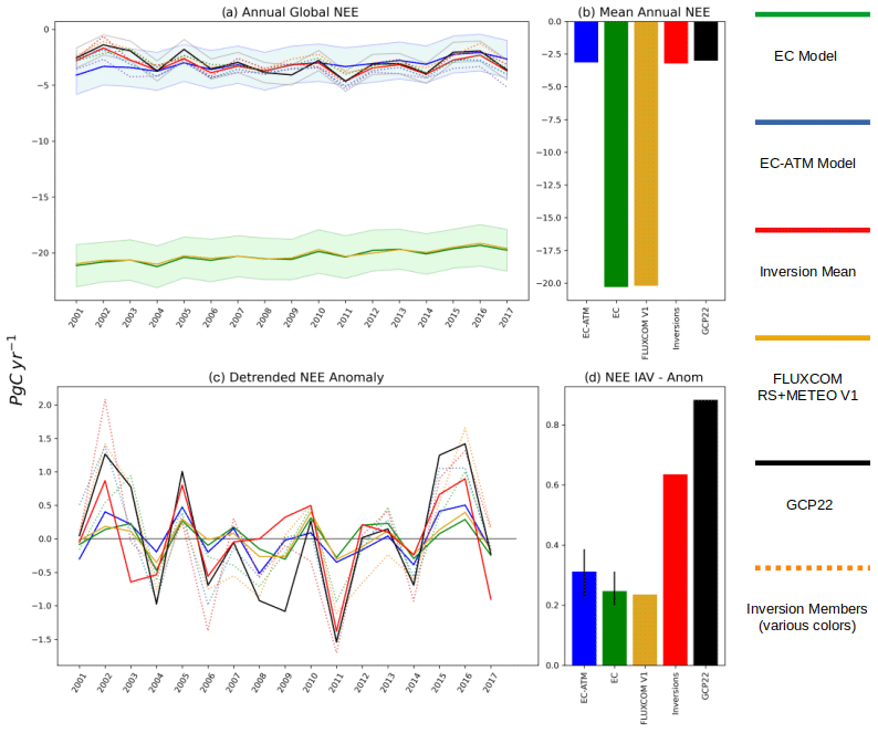
Figure 2 Panel (a) is the global annual NEE (in Pg C yr⁻¹). The blue line is the EC-ATM ensemble mean across the 10 members. The blue shaded area is the EC-ATM uncertainty across the ensemble (±1σ). The green line is the EC ensemble mean across the 10 members. The green shaded area is the EC-ATM uncertainty across the ensemble (±1σ). The red line is the ensemble mean of the atmospheric inversions. The individual inversions are shown in dotted lines. The black line is the GCP22 residual land sink. The grey shaded area is the published GCB22 uncertainly. The yellow line is the ensemble mean of FLUXCOM RS+METEO V1. Panel (b) is the annual mean across 2001–2017. Panel (c) shows the detrended anomalies (in Pg C yr⁻¹). Panel (d) shows the magnitude of IAV, estimated as the standard deviation of detrended annual anomalies. The bars on the EC and EC-ATM bars indicate the spread of IAV across the 10 members.

The GCB22 results are not available at the RECCAP2 regional level, so to assess the performance of the models at regional scale we use the ensemble of atmospheric inversions for comparison. We acknowledge that the estimates are not fully independent, since they are based on the same data used to train our model, but we expect our training approach (see Sect. 3.4 above) to make NEE estimates from the EC-ATM model sufficiently distinct from the ensemble mean of atmospheric inversions that is not used in directly the training.

Figure 2b shows that the mean anomaly of NEE estimated by the EC-ATM model largely captures the sign of the atmospheric inversion and GCB22 anomalies, but the IAV is still underestimated by both the EC-ATM and EC models, which is a persistent issue with the FLUXCOM approach (see Jung et al., 2020 for full discussion) as well as a general issue with statistical learning. The EC-ATM annual mean is strongly correlated with the detrended standardized annual anomalies of the atmospheric inversion ensemble mean (R² of 0.67), producing very similar results to the FLUXCOM RS+METEO results (Fig. 2b).

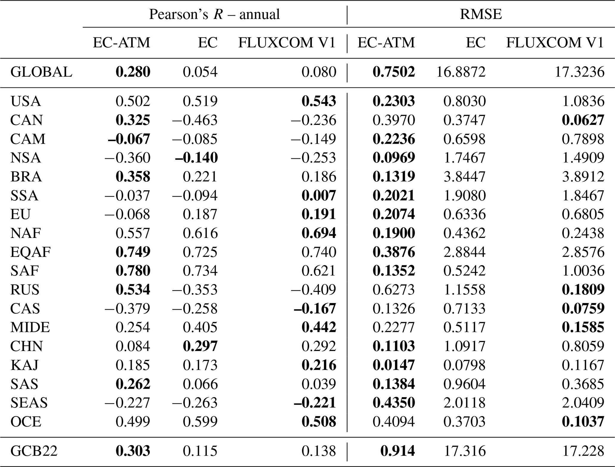
In annual regional results (Table 2), the EC-ATM model generally outperforms the EC and FLUXCOM RS+METEO models in the tropics, with more mixed results in the extratropical regions. There is an improvement in RMSE for most regions. The RMSE for Brazil improves over the FLUXCOM RS+METEO, going from 3.89 to 0.13 Pg C yr⁻¹, and Europe improves from 0.68 to 0.21 Pg C yr⁻¹. The EC-ATM model appears to have lower performance for boreal regions compared with FLUXCOM. Both Canada (CAN) and Russia (RUS) have higher RMSE compared with the inversion ensemble mean (0.63 Pg C yr⁻¹ for the EC-ATM compared with 0.18 Pg C yr⁻¹ for FLUXCOM in RUS). The correlation does not show clear or systematic improvement. The Pearson's R for most regions are largely similar (see result for the USA, Equatorial Africa (EQAF), and Southeast Asia (SEAS)). This is consistent with the overall low performance in capturing the IAV signal with data-driven flux models. Of note is the fact that while the boreal regions have higher errors, they have stronger correlations (0.53 Pg C yr⁻¹ for the EC-ATM compared with −0.41 Pg C yr⁻¹ for the EC in RUS), indicating a larger magnitude of error but better estimation of the monthly ecosystem dynamics.

Table 2 Results of annual NEE aggregated by regions. Pearson's correlation coefficient (R) of the annual integral of NEE from the inversion ensemble mean with the machine-learned model estimates from EC-ATM, EC, and FLUXCOM. The final row is the Pearson's R and RMSE globally for the three models compared with the GCB22 results. Values are given in units of Pg C yr⁻¹. Bold numbers denote the best-performing model by region and metric. Country and region abbreviations are expanded in Appendix Table A1.

4.2 Monthly and seasonal variability

We evaluate the performance of the EC and EC-ATM models in capturing the overall temporal variability in NEE by estimating the normalized Nash–Sutcliffe model efficiency (nNSE) metric for regional monthly NEE values over all years (2001–2017) (Fig. 3). Normalized Nash–Sutcliffe model efficiency is a transformation of standard Nash–Sutcliffe metric, which assesses the predictive skill of a model in regard to a reference set of values, in this instance, the monthly regional integrals of the atmospheric inversion ensemble. The normalization transforms the range of the metric from $(-\mathrm{\infty },\mathrm{1})$ to (0,1). An nNSE of 1.0 represents perfect skill where the EC-ATM or EC perfectly reproduce this reference. An nNSE of 0 represents no skill. An nNSE of 0.5 is where the model predicts the reference better than repeating the annual regional mean integrals of the atmospheric inversion ensemble. Figure 3 shows that in almost all regions the EC-ATM model is better able to predict the atmospheric inversions than the EC model.

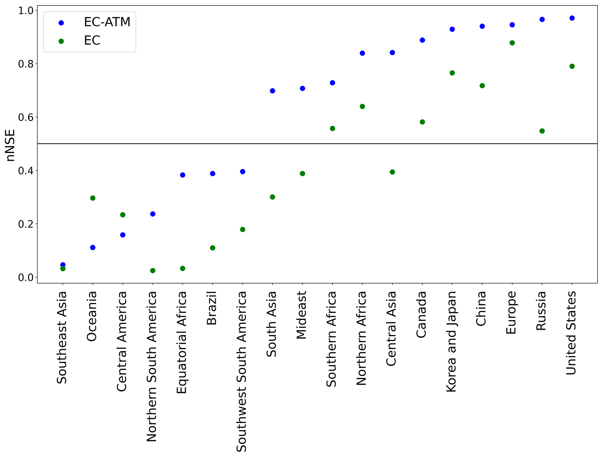
Figure 3 Normalized Nash–Sutcliffe model efficiency over all regions ordered by EC-ATM performance. An nNSE of 1.0 represents perfect skill where the EC-ATM or EC perfectly reproduce the monthly regional integrals of the atmospheric inversion ensemble. An nNSE of 0 represents no skill. An nNSE of 0.5 is where the model predicts the reference better than repeating the annual mean of the atmospheric inversion ensemble.

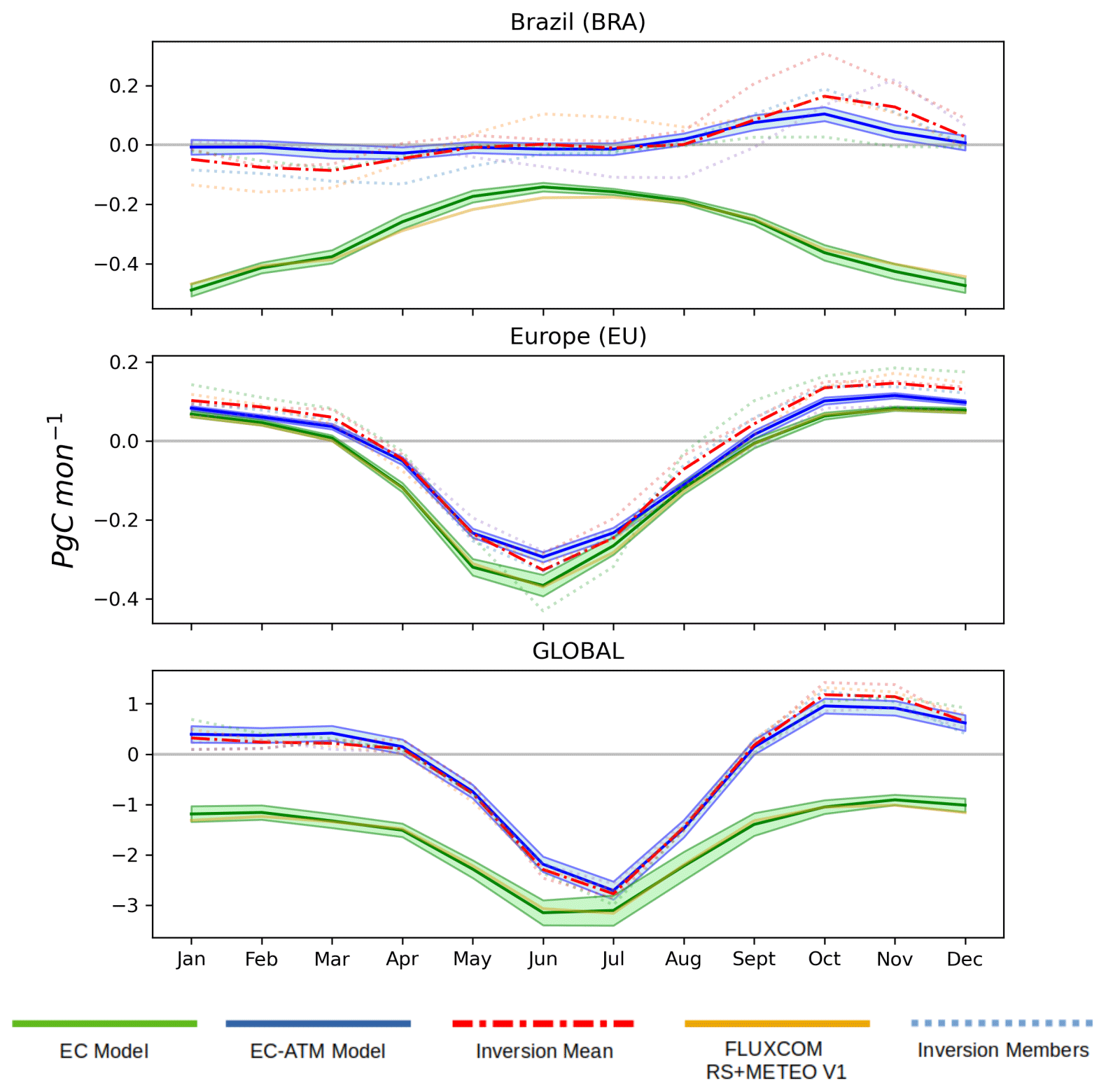
Figure 4 Mean seasonal cycle of ensemble mean of monthly NEE (Pg C per month) for a representative tropical region (Brazil, BRA), extratropical region (Europe, EU), and the globe for the years 2001–2017. The solid line shows the ensemble mean, and the shaded region is the mean ± the ensemble standard deviation.

The mean seasonal cycle (MSC) of the global NEE estimated by the EC-ATM model shows a clear adjustment towards the atmospheric inversion ensemble mean and away from the estimates from the EC model and FLUXCOM RS+METEO results, consistent with the rationale to use a double-constraint approach (Fig. 4). In extratropical regions (e.g., EU in Fig. 4) the MSC of the EC-ATM is very close to the FLUXCOM RS+METEO and inversion ensemble mean results. But globally and in tropical regions the MSC shows a meaningful improvement (Table 3). The range of the global MSC (3.66 Pg C) is closer to the atmospheric inversion ensemble mean (3.88 Pg C) compared with 2.24 Pg C in the EC model (Fig. 4). The EC-ATM MSC has an RMSE of 0.13 Pg C compared with 1.54 Pg C for FLUXCOM RS+METEO and 1.5 Pg C for the EC model. The seasonality of the EC-ATM inferred flux is also closer to that of the atmospheric inversion ensemble mean, although the EC-ATM model appears to underestimate the source during the Northern Hemisphere winter and conversely overestimate it in the Northern Hemisphere early spring (Appendix Fig. C1).

Table 3 Results of monthly NEE aggregated by region: Pearson's R and RMSE of the monthly time series of regional and global integrals over the period 2001–2017 and the corresponding monthly NEE from atmospheric inversions, the Pearson's R of the regional and global mean seasonal cycle (MSC) of NEE, the RMSE of the MSC relative to the inversion mean, and the model MSC. FLUXCOM refers to the RS+METEO V1 product (Jung et al., 2020). Bold numbers denote the best-performing model by region and metric. Country and region abbreviations are expanded in Appendix Table A1.

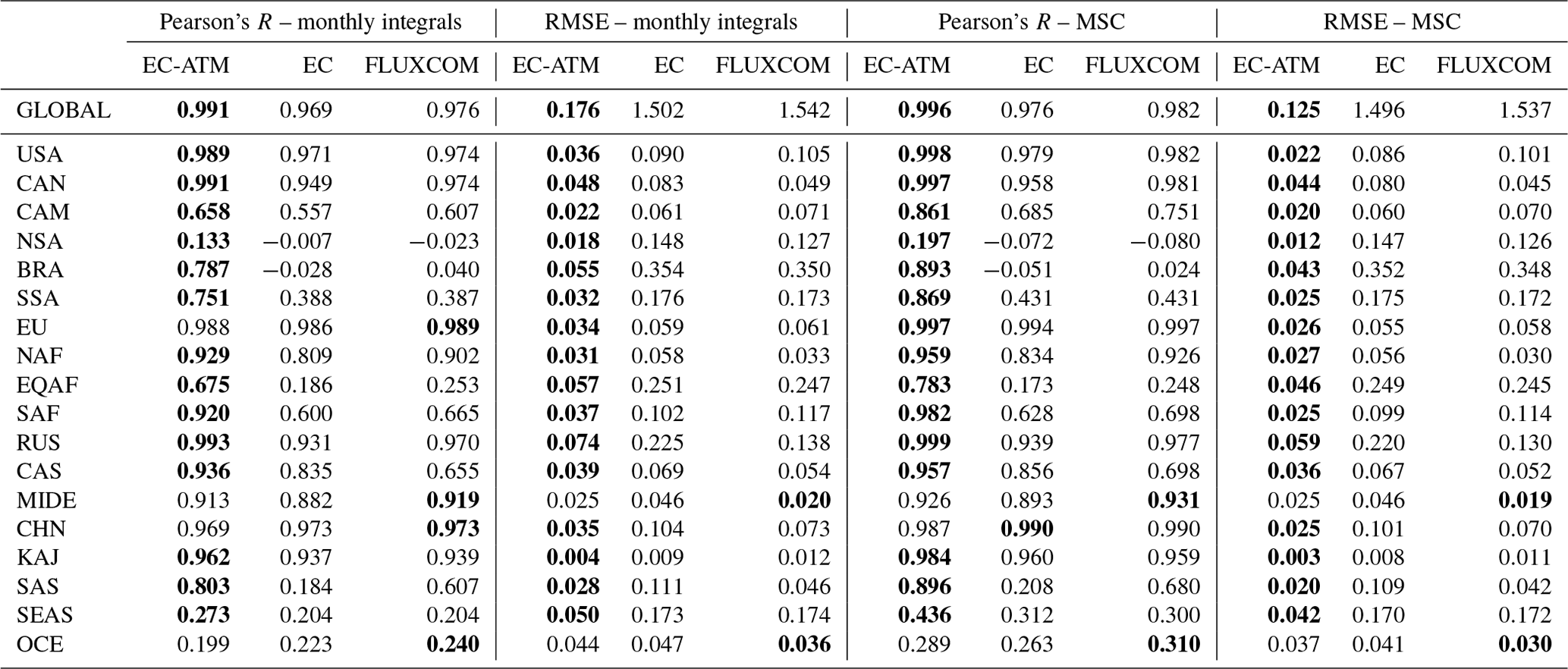
The EC-ATM model shows an improvement in the global RMSE of monthly NEE from 1.54 Pg C per month for the EC mean to 0.13 Pg C per month for the EC-ATM model mean (Fig. 3). The regional monthly performance of the EC-ATM model shows improvements in both the monthly time series and MSC for almost all regions (Table 3). In extratropical regions the improvements are small. The EC-ATM NEE for Canada (CAN) has a monthly Pearson's R of 0.991 compared with 0.969 for the EC model, and 0.949 for FLUXCOM RS+METEO. However, in tropical regions the change is much larger. The EC-ATM NEE for Brazil (BRA) has a monthly Pearson's R of 0.787 compared with 0.028 for the EC model and 0.040 for FLUXCOM. Regions where the EC or FLUXCOM outperform the EC-ATM results are all in regions where all three models perform very similarly.

In Appendix Fig. C1 impact of the atmospheric information on the seasonality of the MSC is quite clear. In tropical regions (e.g., Central America (CAM), South Asia (SAS), BRA) the EC-ATM result has a very different seasonality than the EC and FLUXCOM RS+METEO results, including different ranges and means. The correspondence between the inversion ensemble mean and EC-ATM MSC is close, but the differences reflect the balance between eddy covariance and atmospheric information during model training, and the higher uncertainty between inversions in tropical regions. The difference between the EC model MSC and the FLUXCOM RS+METEO MSC can be attributed to different initial model states. The EC model is an analog for a member of the FLUXCOM RS+METEO ensemble, the mean of which is used here for comparison. In the extratropical regions, the estimates of NEE MSC by EC and EC-ATM are very similar in range and seasonality.

These results indicate that additional atmospheric constraints are indeed reflected in the EC-ATM model at seasonal and continental scales, i.e., the scales where atmospheric data are most informative.

Figure 4 shows the following two selected regions: (1) Brazil, which is representative of tropical regions with sparse EC observations and potential systematic bias in the EC data, and (2) Europe, which is representative of extratropical regions with a dense EC network. In Brazil, the EC-ATM model mean shows closer temporal evolution and magnitude of the MSC to the mean of the atmospheric inversions, than the EC model estimates. At a monthly time step, the correlation of the EC-ATM with the atmospheric inversions is largely similar with the FLUXCOM RS+METEO V1 (0.99 and 0.98, respectively), only out-performing it in some tropical regions, such as BRA, EQAF, and Southwest South America (SSA). The results in Europe are very similar for the EC, EC-ATM, and FLUXCOM models, with all three producing a MSC very close (RMSEs of 0.055, 0.026, 0.058 Pg C per month respectively) to the ensemble mean of the atmospheric inversions. Overall, the EC-ATM shows a persistent improvement in the RMSE of the MSC (relative to the inversion mean) across almost all regions (Table 3).

4.3 Spatial variability

The spatial patterns of mean annual NEE estimated by the EC-ATM model are considerably different from those estimated by the EC model (Fig. 5). Specifically, the EC model estimates a strong mean annual sink across the tropics, while the EC-ATM model estimates more heterogeneous patterns, with sources and sinks across the tropical regions. For example, in the Amazon, the EC model estimates a strong sink of more than 1.5 Tg C yr⁻¹ per pixel, while the mean of the atmosphere inversions shows a weak and rather homogeneous source of around 0.1–0.2 Tg C yr⁻¹ per pixel, and the EC-ATM model infers a mixed pattern of strong sinks and sources. The noisy pattern in the Amazon basin estimated by the EC-ATM model may indicate some instability of the model or an amplification of the limited signal coming from the low density of eddy-covariance sites. In tropical Africa, the EC-ATM model shows an annual source while both the EC model and the atmospheric inversions estimate a moderate to strong sink.

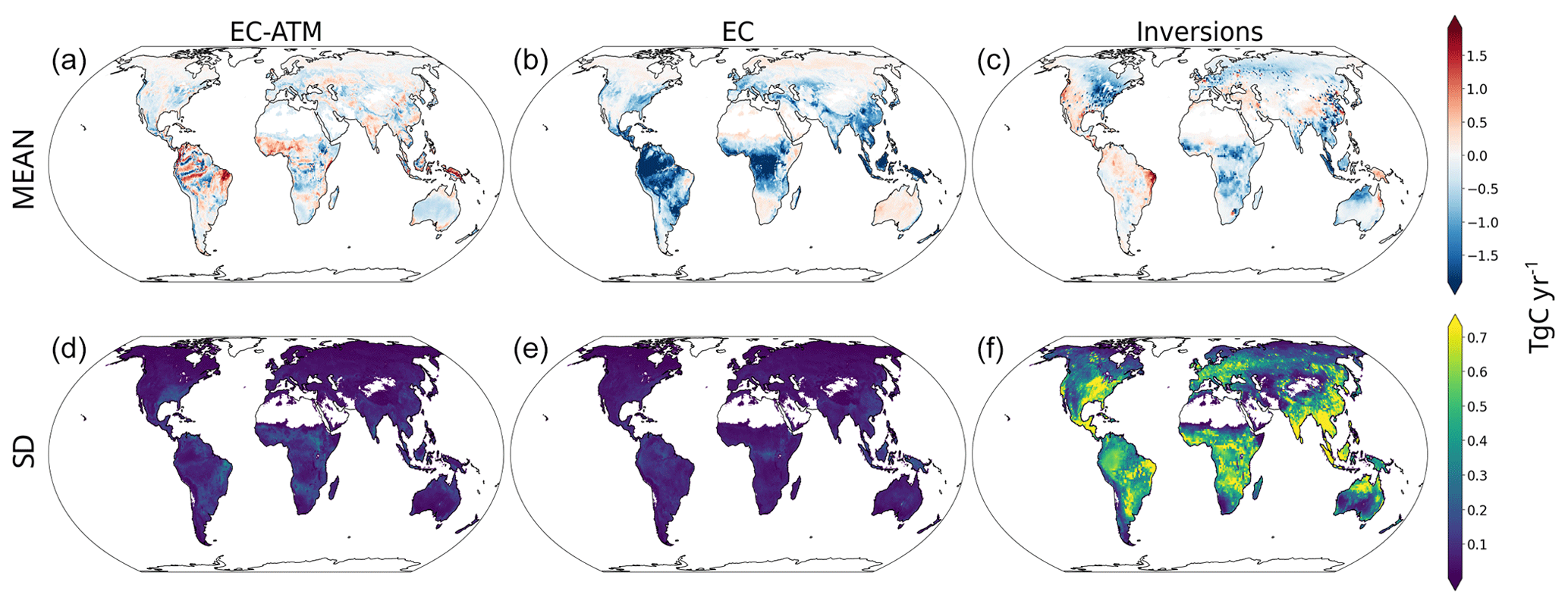
Figure 5 Mean (a–c) and standard deviation (d–f) of the ensemble mean annual NEE from the EC-ATM and EC models compared to the ensemble mean of the atmospheric inversions. Panels (b)–(c) show the per-pixel mean of the annual NEE. Panels (d)–(f) show the per-pixel standard deviation of the annual NEE (in Tg C m⁻² yr⁻¹).

It should be noted that there is a known large disagreement between atmospheric inversions in the tropical regions and the location of sources and sinks varies strongly across atmospheric inversion models (Friedlingstein et al., 2022; Gaubert et al., 2019; Palmer et al., 2019). The integration of bottom-up constraints in a unified model (EC-ATM) is not likely to resolve these spatial differences across top-down estimates but rather to achieve NEE that is in between top-down and bottom-up approaches, as exemplified by the patterns in Fig. 5.

Similar to the results of global IAV, the EC-ATM and EC model estimates display much weaker year-to-year variability in annual NEE compared to the mean of inversions (Fig. 5). While atmospheric inversions estimate IAV of about 0.5–0.8 Tg C yr⁻¹ in many tropical pixels, eastern North America, and western Eurasia, the EC and the EC-ATM models does not exceed 0.38 and 0.42 Tg C yr⁻¹, respectively. This difference highlights the difficulty that both the EC and EC-ATM models have in capturing the magnitude of the interannual variability, as also shown in Jung et al. (2020).

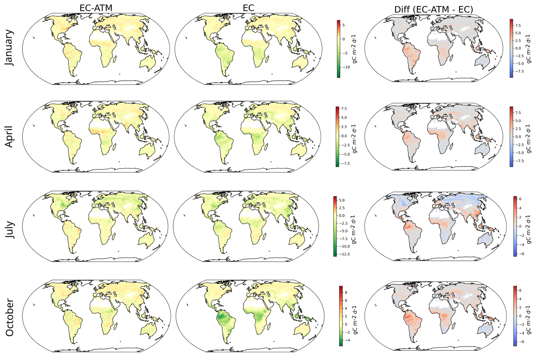
Figure 6 Monthly mean fluxes for 2001–2017 for 4 selected months. The left column shows the EC model results, the middle column shows EC-ATM model results, and the right column shows the difference between them (EC-ATM − EC).

We further evaluate the spatial distribution of NEE for 4 selected months representative of different seasons: January, April, July, and October (Fig. 6). The distribution of the EC-ATM mean monthly flux from years 2001 to 2017 shows the reduced flux in the tropics throughout the year (red regions in the right column). The EC model estimates a stronger sink than the EC-ATM model in the tropical regions and over the whole year and especially during the wet season (October). On the contrary, the EC-ATM model indicates a stronger sink in the Northern Hemisphere during boreal summer (North America, Europe, northern Eurasia in July), and in semi-arid regions in Southern Africa and Oceania during most of the year.

The spatial distribution of mean annual and monthly NEE estimated by the EC-ATM model is largely consistent with that estimated by the EC model, while reducing the tropical sink. EC-ATM shows some irregularities in the spatial patterns where there is insufficient information in either the eddy-covariance data or atmospheric inversions to robustly localize the NEE.

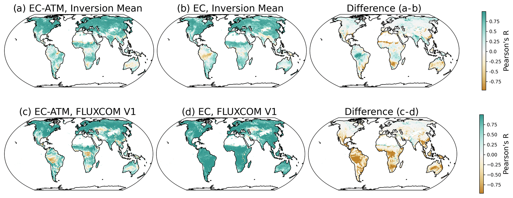
Figure 7 Spatial patterns of the per-pixel temporal correlation (Pearson's R) between EC-ATM and EC monthly NEE and the atmospheric inversion monthly mean (a, b) and FLUXCOM RS+METEO V1 monthly results (Jung et al., 2020) (c, d). Panels (a–b) and (c–d) show the difference between the EC-ATM and EC correlation.

We then compare the monthly pixel-level correlation between NEE estimated by the EC and EC-ATM models and by the atmospheric inversions (Fig. 7). Note that pixel-level estimates of NEE by atmospheric inversions are not expected to be robust. Nevertheless, this analysis allows us to better understand how the EC-ATM model learns spatiotemporal variability in NEE. We find that both the EC-ATM and EC models correlate well with the inversion mean in the extratropics where both products are better constrained by observations, with temporal correlations greater than 0.5. In the tropics, the EC model has a negative correlation with the inversion mean in the tropics (ca. −0.4), while the EC-ATM model estimates weak but positive correlations with the inversion mean (ca. 0.2–0.4). While there is low confidence in atmospheric inversions' estimates at the pixel level; nevertheless, this result shows that including regionally aggregated top-down constraints in the EC-ATM model results in changes to the temporal variability also at pixel level (where EC-ATM pixel-level variability departs from FLUXCOM RS+METEO V1, lower-right panel in Fig. 7). This demonstrates that the model is not simply learning a bias correction but a new pattern of land flux that incorporates some but not all of the information in the atmospheric inversions.

4.4 In situ model comparison

The comparison of EC and EC-ATM modeled NEE at the eddy-covariance sites (Fig. 8) shows that the EC-ATM and EC models have a similar RMSE with observed NEE globally. Both the EC and EC-ATM model RMSE performances of 1.349 and 1.321 g C m⁻² d⁻¹, respectively, are similar to the median results of RMSE for NEE using the setup in Tramontana et al. (2016) of 1.298 g C m⁻² d⁻¹. The optimization of the model hyperparameters (i.e., number of neurons, learning rate) for EC-ATM performance based on the large-scale top-down constraints may lead to a slight underperformance when these are also applied in the EC model.

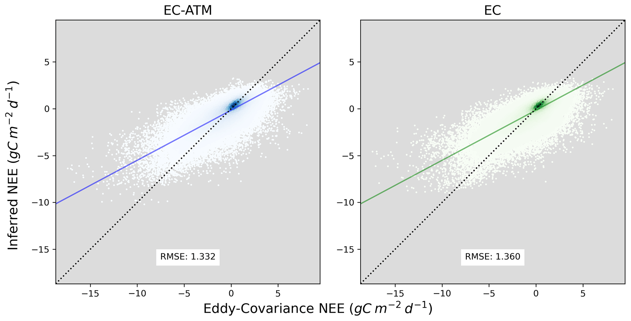
Figure 8 Comparison of inference of daily NEE from the EC-ATM and EC models with corresponding tower observations, across the whole set of available eddy-covariance observations. The x axes show the eddy-covariance observations (in g C m⁻² d⁻¹), the y axes show the NEE EC-ATM and NEE EC (in g C m⁻² d⁻¹). The blue and green lines are the line of best fit for the EC-ATM and EC results respectively, and the dotted line is the x=y line.

The RMSE of inferred NEE at the eddy-covariance tower level for the EC and EC-ATM models is very similar across tower sites globally, and by the PFT that is most represented in the pixel, or majority PFT. A breakdown of tower performance by the pixel-majority PFT is available in the Appendix C2. This may indicate that, for the majority of tower sites, the information of regional NEE by atmospheric inversions acts as a complementary constraint, improving, albeit very slightly, the EC-ATM model estimates of NEE across the full set of eddy-covariance observations considered here.

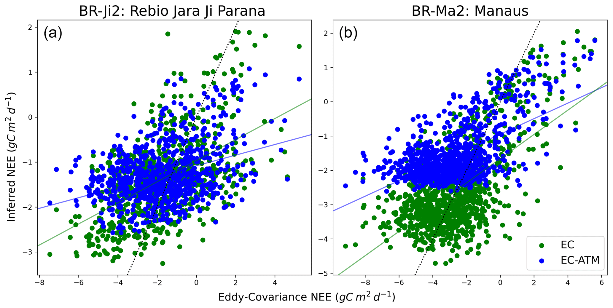
Figure 9 Comparison of EC and EC-ATM model output at two Brazilian eddy-covariance sites. The y axes are the NEE EC-ATM and NEE EC (in g C m⁻² d⁻¹), the x axes are the eddy-covariance observations (in g C m⁻² d⁻¹). The dotted black line is the x=y line. The blue and green lines are the line of best fit for the EC-ATM and EC results, respectively. This figure shows the different learned response in the EC-ATM model (blue) from the atmospheric constraint at a tower location compared with the EC model and the tower observations. Panel (a) shows where the learned response is similar. Panel (b) shows where the atmospheric constraint was not complementary with the eddy-covariance constraint, and the model has a larger bias than the EC model when compared with tower observations.

At individual tower sites the EC-ATM model can learn different responses than the EC model. At tower BR-Ji2 (see Fig. 9a) the EC and EC-ATM models show very similar skill in capturing variability of NEE measurements, with both estimating a smaller sink compared to the tower observations. At BR-Ma2 (see Fig. 9b), the EC-ATM model learns an overall smaller sink, compared with the EC model and tower observations, increasing the bias relative to NEE measurements at the tower site compared with the EC. This demonstrates that the information from the atmospheric constraint can act as a non-complementary constraint. Here it reduces the accuracy of the EC-ATM model at the EC tower level as it learns the smaller regional tropical sink from the atmospheric information.

5 Discussion

In this study, we aimed to evaluate the hypothesis that combining top-down and bottom-up estimates of land–atmosphere carbon fluxes could contribute to improve the estimates of regional and global land carbon sinks (Jung et al., 2020; Anav et al., 2015). To do this, we created a data-driven flux model trained on the observed NEE from eddy-covariance sites. Then, in parallel, we tested the effect of adding an additional top-down constraint based on the regional integrals of NEE from an ensemble of atmospheric inversions to the model's objective function used in NEE optimization. Our results show that adding regional atmospheric constraints to a bottom-up data-driven flux model improves NEE estimates from monthly to inter-annual and local to global scales. This approach minimizes the limitations of both top-down and bottom-up systems. It yields a model that preserves the local, small-scale view of the bottom-up approach while bringing the regional and globally integrated results in line with other best estimates of NEE.

At the global annual level the EC-ATM results show much closer correspondence with the GCPB22 residual land sink (Fig. 2). This indicates that the EC-ATM model, which runs at the pixel level with no additional larger spatial or temporal context, has learned a new response from the drivers at the ecosystem level, leading to a more realistic global integral of NEE. This demonstrates the efficiency of the atmospheric constraint, and its ability to appropriately transmit information from the region down to the ecosystem level. At the monthly regional level, the EC-ATM outperforms the EC and FLUXCOM RS+METEO V1 results in Pearson's R and RMSE (see Table 3). The EC-ATM model improves the seasonal pattern and magnitude of the MSC across regions (see Fig. C1) when compared with other the EC model and FLUXCOM. This indicates that the additional information does not create a simple global or regional bias-correction term, but rather a more complex constraint that varies effectively in both space and time. This is also evident in the correction at some tower locations (Fig. 9). The difference between the observed and inferred NEE by the EC and EC-ATM models at specific EC towers demonstrates that the atmospheric information acts locally during training and can provide both complementary and non-complementary information to the constraint from eddy covariance.

The impact of the complementary or non-complementary function of the combined constraints in the final model can be seen in the differences between tropical and extratropical regions. In general, the EC, EC-ATM, and FLUXCOM results are quite similar in extratropical region, especially in the northern extratropics where the eddy-covariance network is dense and the eddy-covariance data collection method is more robust, and the atmospheric inversions have lower uncertainty (see USA and EU data in Tables 2 and 3 and Fig. C1). Here, the two constraints are providing complementary information, and the eddy-covariance data appears sufficient. In tropical regions, where the eddy-covariance record is sparse, eddy-covariance measurements are more prone to error, and the inversions are more uncertain, the EC-ATM model learns a temporally and spatially dependent mixing of the two constraints, which may or may not work in a complementary way. The results for Brazil (BRA) show that the EC-ATM model has corrected its response at the annual and seasonal time frame, but spatially (Figs. 7, 5) we see that the spatial and temporal distribution of NEE is different both from the inversion ensemble and FLUXCOM RS+METEO V1.

We note that this approach only partly resolved some of the weaknesses of data-driven models. The EC-ATM shows very limited improvement relative to the EC model and the FLUXCOM RS+METEO V1 (Jung et al., 2020) in reducing the underestimation of NEE IAV magnitude, compared with atmospheric inversions and the land sink from global carbon budgets (Friedlingstein et al., 2022). This may be due to the fact that the optimization of the neural network and formulation of the driver variables is the same as used in FLUXCOM RS+METEO V1. Specifically, the driver variables in both the EC and EC-ATM models are largely based on mean season cycles of the underlying remotely sensed data (Table A2) or data derived from seasonal metrics, such as the minimum and range of the mean season cycle of water availability. This limits the amount of information available for the EC or EC-ATM model to learn about the IAV component of the signal. Moreover, the magnitude of IAV is small compared to the seasonality of NEE. Therefore, since we optimize fluxes at sub-annual timescales (daily for training term 1 and monthly for training term 2), the EC-ATM model may tend to optimize for the signal with larger contribution to the objective function, i.e., the seasonal variability, rather than IAV.

Another reason for the IAV underestimation in both EC and EC-ATM models might be missing information in the training set, for example due to the fact that semi-arid tropical regions, where the NEE is strongly impacted by climate variance and that account for a very large portion of IAV in the global land sink (Ahlström et al., 2015; Poulter et al., 2014), are under-represented in the FLUXNET network. We expect the regional top-down constraint by atmospheric inversions to partly improve this, but atmospheric inversions tend to assign less IAV to the tropical semi-arid regions than land surface models used in global carbon budgets (Piao et al., 2020) and also tend to infer lower sensitivity of NEE IAV to tropical water and temperature variability (Wang et al., 2022).

While model structure could contribute to this issues, experiments (not shown) with varying architecture (number of neurons, number of layers, layer connectivity), activation functions, and loss terms of the EC and EC-ATM models were not successful in reducing the bias in the magnitude of NEE IAV. We also conducted sensitivity experiments on the objective function both structurally and in its formulation. Structurally, the number of regions included in the atmospheric term at each step and the number of months included at each step were varied. The best results, as indicated in the methods, was considering a full year for each region at each training step.

5.1 Uncertainty in top-down constraints

The sparsity of observations concerns not only the FLUXNET network but also the network of atmospheric monitoring sites used by atmospheric inversions. Given the small number of tropical observations considered in top-down constraints and the inherited uncertainty from priors and transport models, which are not directly managed by the system in this study (Baker et al., 2006), the EC-ATM model result might still be prone to large uncertainties in the tropics. Here, we discuss the handling of uncertainty in the EC-ATM model in more detail.

The system presented in this study is still dependent on the priors and transport models in the underlying atmospheric inversions and is still subject to the underlying uncertainty of these data, particularly in the tropics where both bottom-up and top-down systems lack sufficient observations. During training, the EC-ATM model tries to account for uncertainties in two ways: the error between the inference and the inversion data is normalized in the loss atmospheric loss term by the spread of the inversion estimates by time and region, which reflects uncertainty across inversion models (Eq. 10); additionally, the model learns to weight the objective term relative to the estimated uncertainty in the atmospheric loss term, which should tend to reduce the weight where there is larger systematic disagreement between inversion systems (Eq. 12).

We perform a “one-against-many” sensitivity analysis, where we trained several models with the atmospheric constraint coming from either one inversion (zero spread), two randomly selected inversions, or three randomly selected inversions. This analysis, shown in the Appendix​​​​​​​ (Figs. C3, C4, C5) allows us to evaluate how the specific inversion NEE estimates interact with the loss mixing scheme in the model training. In extratropical regions where the eddy-covariance and atmospheric observations are dense, the specific inversion NEE trained on does not critically influence the model response. There is strong correspondence between all EC-ATM instances with individual or smaller groups of inversions and the full inversion ensemble mean. In tropical regions, there is definite movement towards the specific inversion NEE trained on (the dotted lines in Figs. C3, C4, and C5). This response is balanced against the model initialization and the learned weighting scheme during training. At the global level there is a closer agreement between the trained models and the target inversions, as the relative noise of the tropical regions is dampened by the more consistent extratropical regions. As additional inversions are added, there is a tendency for EC-ATM NEE to move closer to the inversion mean, as the target for optimization contains a larger amount of NEE values from the ensemble of inversions. This analysis demonstrates that the EC-ATM model inherits the uncertainty from the ensemble of atmospheric inversions, with the largest uncertainty remaining in the tropical regions where the available observations for both top-down and bottom-up approaches are lacking.

Our results also show the potential for a confounding effect from the training process. The EC-ATM model is a learned statistical response between the drivers and the training data. There are mismatches between the EC-ATM inference of NEE and the atmospheric data used for the top-down constraint. The atmospheric inversion NEE data, despite being adjusted for fossil fuel, fire, and riverine fluxes, still implicitly includes disturbance and trade fluxes, along with other flux components that are not seen by eddy-covariance measurements and are not accounted for in our model. This means that in reducing the loss terms (Eq. 14), these flux components are implicitly incorporated into the EC-ATM inference, although the model lacks the necessary process information that is not included in the drivers. Furthermore, given the statistical nature of the network used and the training process, the data-driven model should not be considered an analog for a process-based model, where individual terms can be more easily backed out. Training using our double constraint should become less confounded as more additional spatially explicit flux components become available. However, despite these data mismatches, training a data-driven flux model using a dual constraint does create a useful estimate of the NEE at multiple scales.

6 Outlook and conclusions

Our study aimed to demonstrate that adding an atmospheric top-down constraint can positively impact the evolution of a bottom-up data-driven flux model during training, leading to meaningful improvement in local to global NEE estimates. The study demonstrated the positive impact of regional atmospheric information on the training of a well-established data-driven flux model (Jung et al., 2020) and the applicability of using observational constraints of NEE at different spatial scales.

In this study, we combined regional integrals of NEE from atmospheric inversions with in situ NEE from eddy-covariance measurements. We note, however, that these could be multiple data streams at different scales (temporal, spatial) or in different formats (grid, point). Incorporating these different data streams would require different model formulations, potentially including neural network architecture and objective functions, as well as data-driven or physics-based bridge models to create the link from the data-driven flux model to these new data.

This multi-scale approach proposed here may allow us to leverage large volumes of additional data for constraining a data-driven flux model. By substituting a physical model for the statistical bridge model used here, a double-constraint data-driven flux model could generate an inference of NEE across diverse temporal and spatial scales. Because, unlike the statistical bridge models, these additional data could vary with the local meteorology, covering a range of biomes, the data-driven flux model would see a more diverse training set. This could improve the performance of the data-driven flux model by learning from a more representative distribution of the driver variables across the land surface. In the future, this logic could be used for a variety of datasets, for example by pairing the archive of eddy-covariance observations with tall-tower observations of the mole fraction of CO₂ or with novel “flux towers in the sky” (Schimel et al., 2019) estimates from satellite retrievals of total column CO₂ (XCO₂).

Appendix A: Data

Table A1 RECCAP2 region ID, names, and abbreviations.

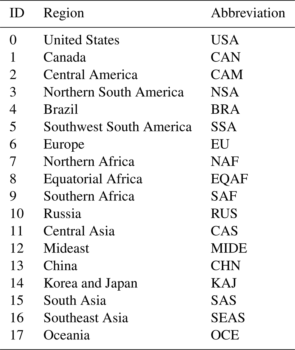
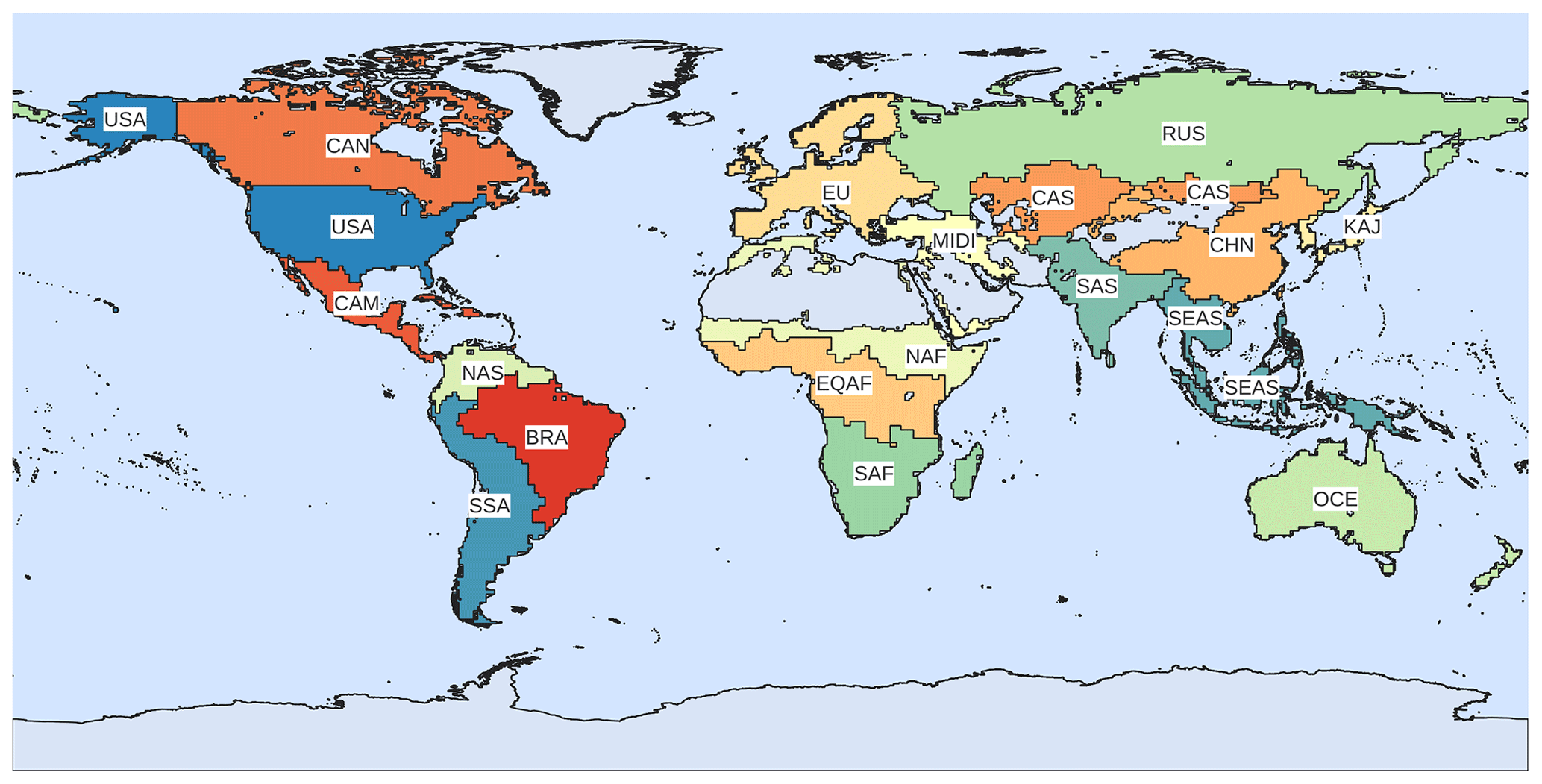
Figure A1 RECCAP2 regions.

Tramontana et al., 2016

Table A2 Driver variables used for the data-driven EC and EC-ATM models and the calculation of the drivers from the base variables above. The global dataset uses only the MODIS and ERA5 data, while the data used at the eddy-covariance sites also uses meteorological observations from the tower instruments. See Tramontana et al. (2016) for a full discussion.

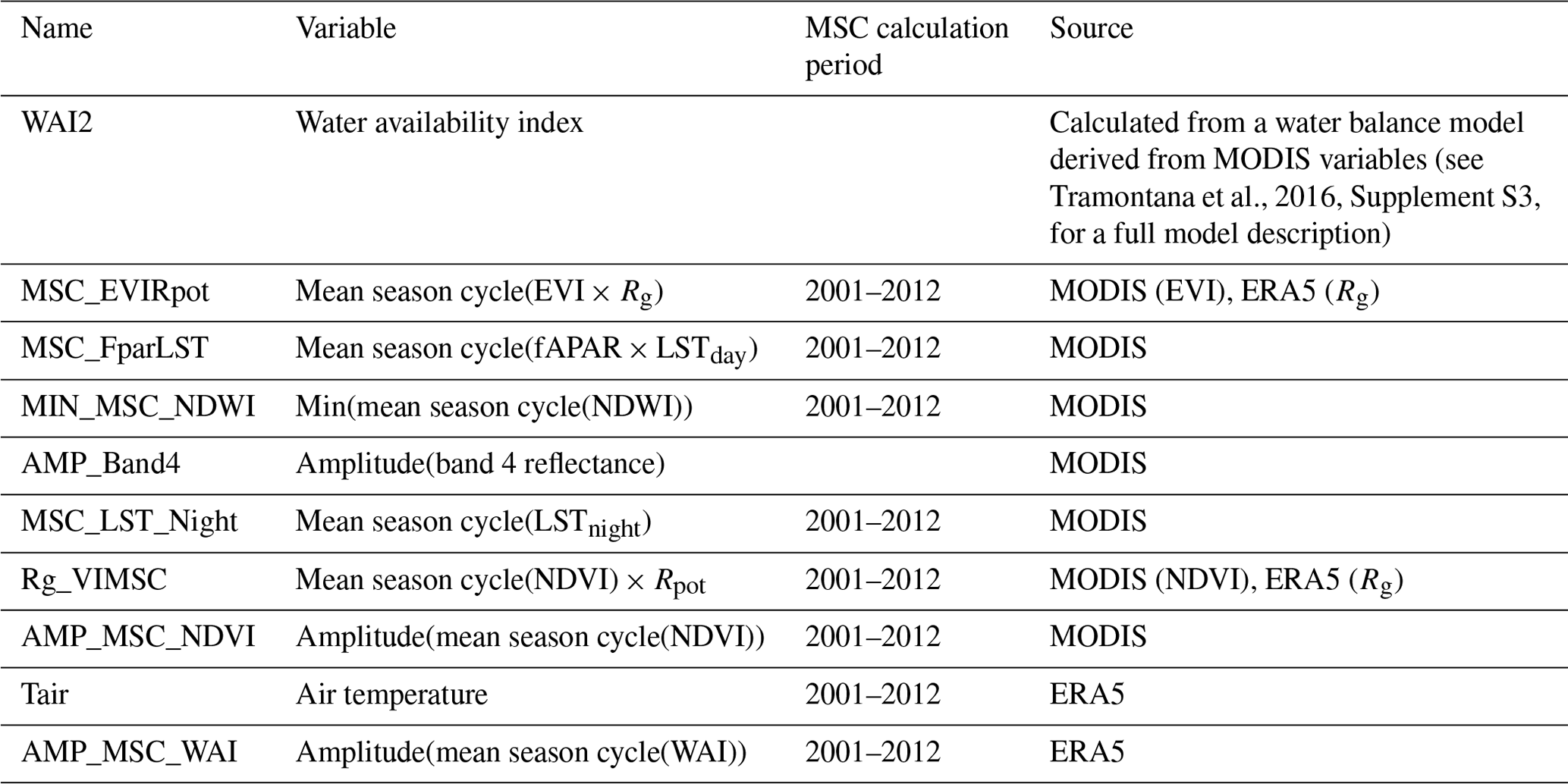
All variables are daily values for 2000–2017 at 0.5° spatial resolution.

Appendix B: Technical implementation

Table B1 Hyperparameters for reported EC and EC-ATM model runs.

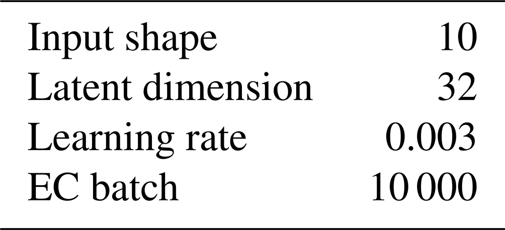
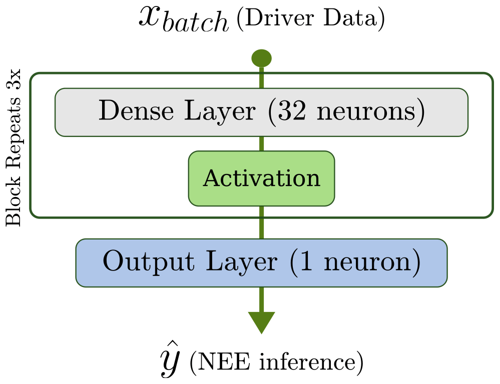
Figure B1 Model architecture showing that the model is a feed-forward neural network or a set of fully connected network layers. The fully connected layers consist of nodes or “neurons”, which are exposed to the output of all neurons in the previous layer. Nonlinearity is introduced by passing each node output through a nonlinear activation function. Our network is a set of three fully connected layers with the ReLU activation function (Agarap, 2019).

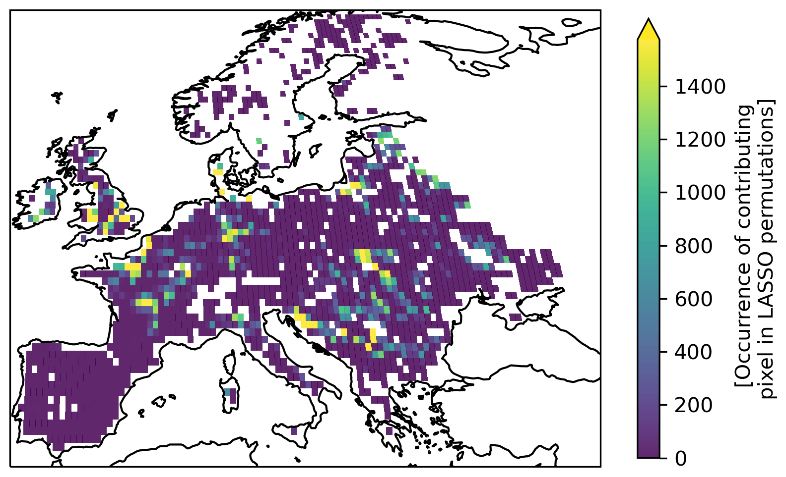
Figure B2 Robustness of contribution pixel selection. A heat map of pixel inclusion in the sparse linear model using Lasso regression is shown. Values represent the log-scaled number of pixel inclusions in the non-zero set of parameters across 500 regressions using a randomized subset of the data. Pixels that are most often included provide a more important constraint on the calculation of a regionally summed NEE, minimizing Eq. (1).

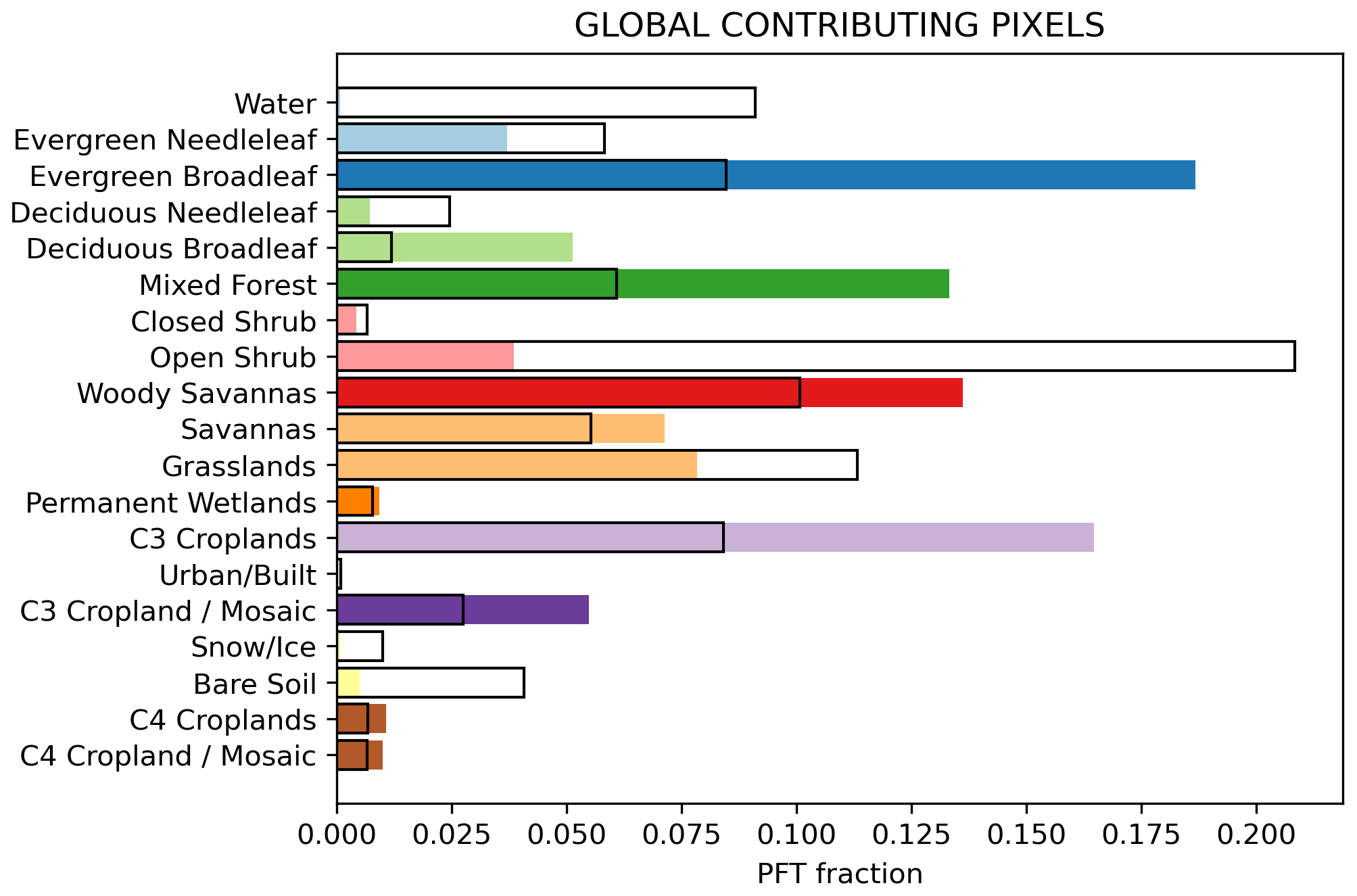
Figure B3 The representation of PFTs across all contributing pixels in all regions. All PFTs are the majority type per pixel. This image shows the relative number of times a certain PFT is included in the optimal set of contributing pixels that construct a regional integral of NEE when selecting from all global land pixels. The black outlines show the proportion of that majority PFT type globally. A per-region analysis of PFT inclusion is available in Appendix B4.

Figure B4 Regional composition of PFT in contributing pixels.

Appendix C: Results

Crisp et al. (2022)Friedlingstein et al. (2022)Gaubert et al. (2019)Ruehr et al. (2023)

Table C1 Estimates of NEE from land from recent studies.

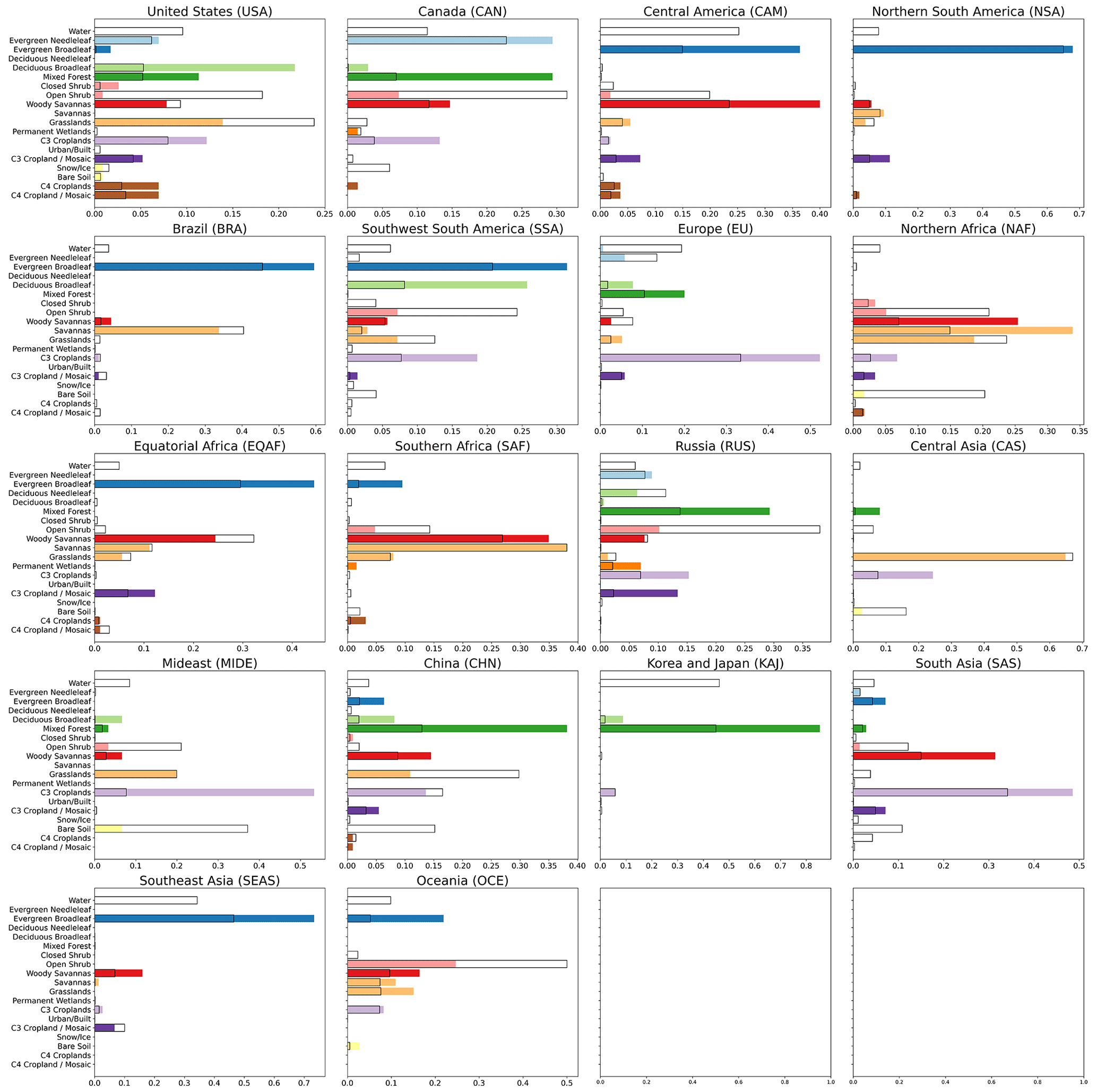
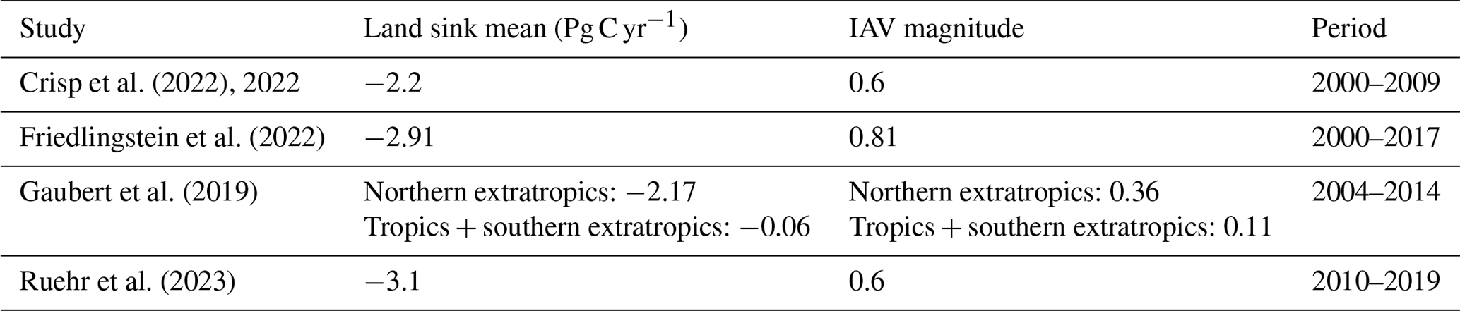
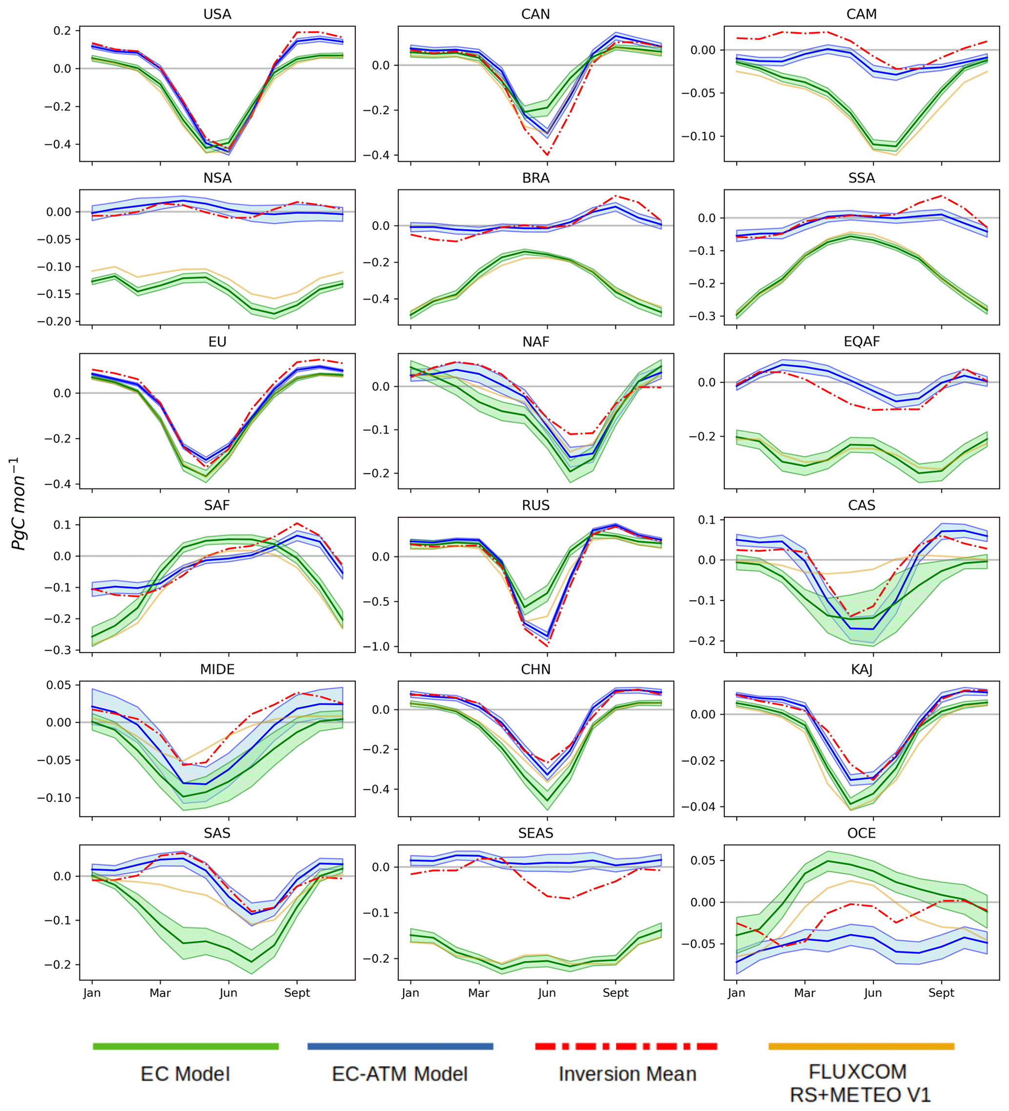
Figure C1 MSC of the ensemble mean of all regions (in Pg C per month). The solid line is the ensemble mean, and the shaded region is the mean ± the ensemble standard deviation.

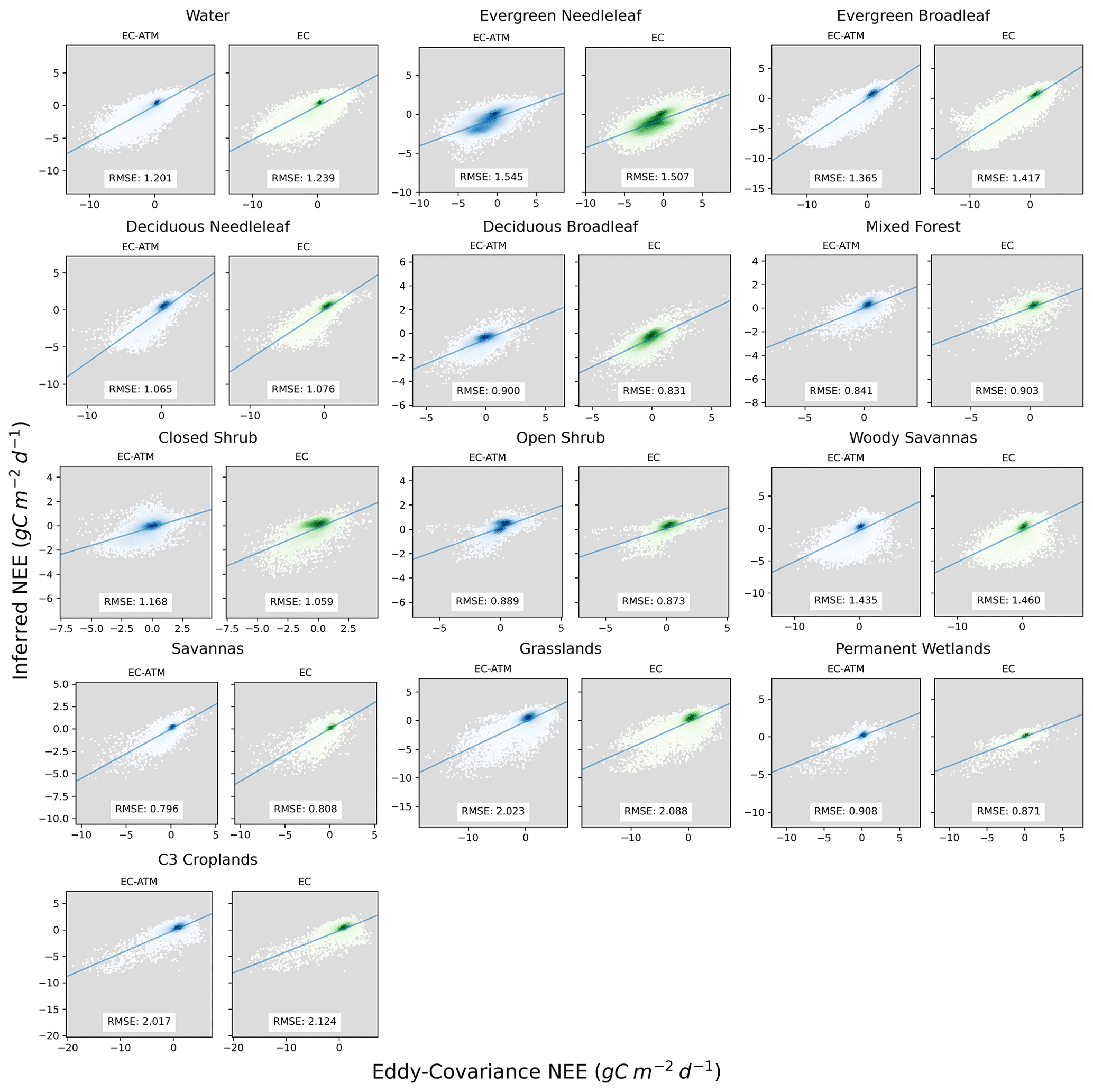
Figure C2 Scatterplots of eddy-covariance NEE (x axis) and inferred NEE (y axis) by PFT and model (ATM-EC, EC).

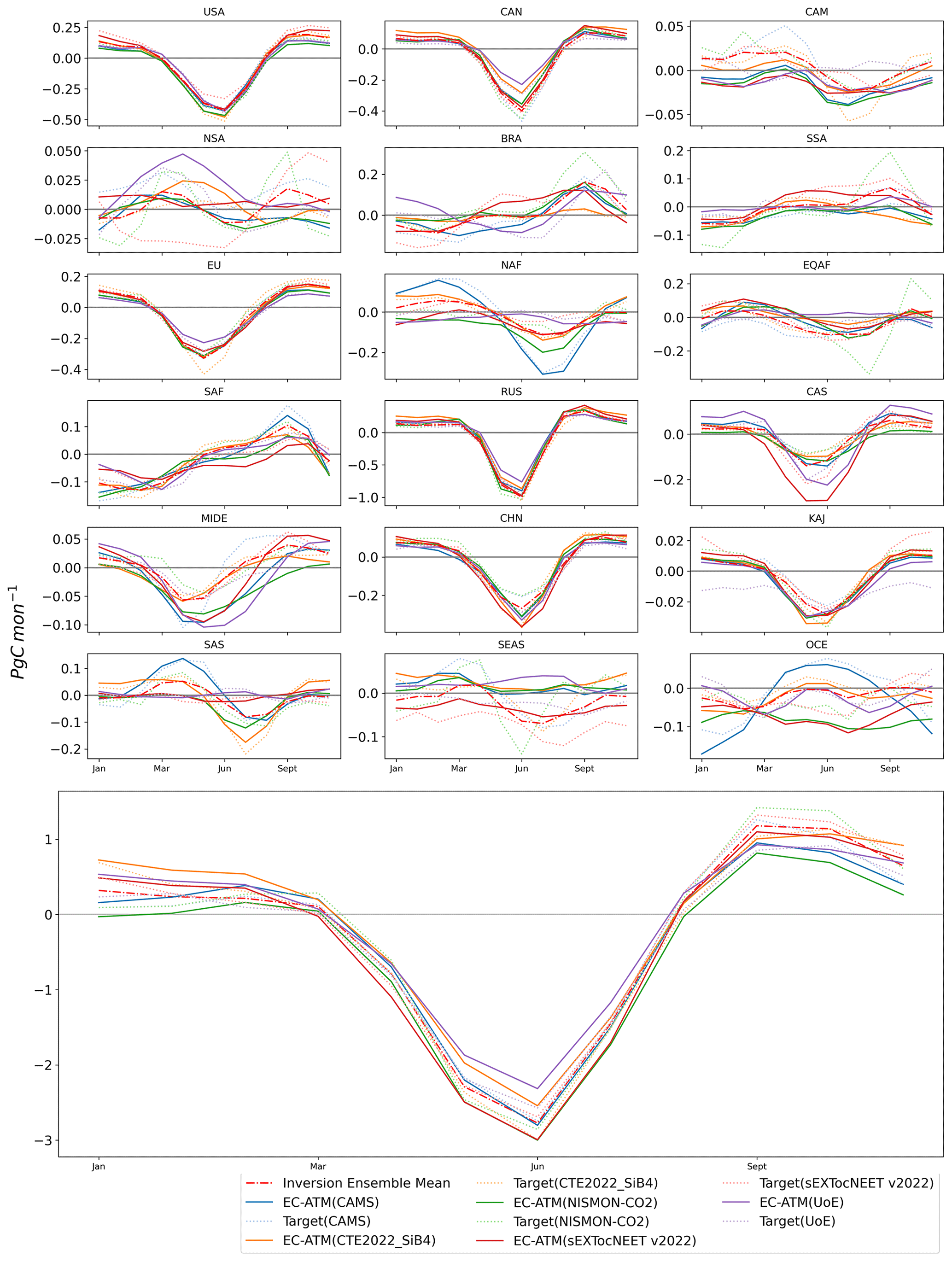
Figure C3 The MSC results for the “one-against-many” training runs. A separate EC-ATM model was trained for each individual inversion system to test the impact of the full ensemble and loss normalization in the full study. The solid lines are the EC-ATM models trained using the named inversion system, and the dotted lines are MSC of the inversion system regional and global integrals. For all panels, the x axis is the yearly cycle, while the y axis is Pg C per month.

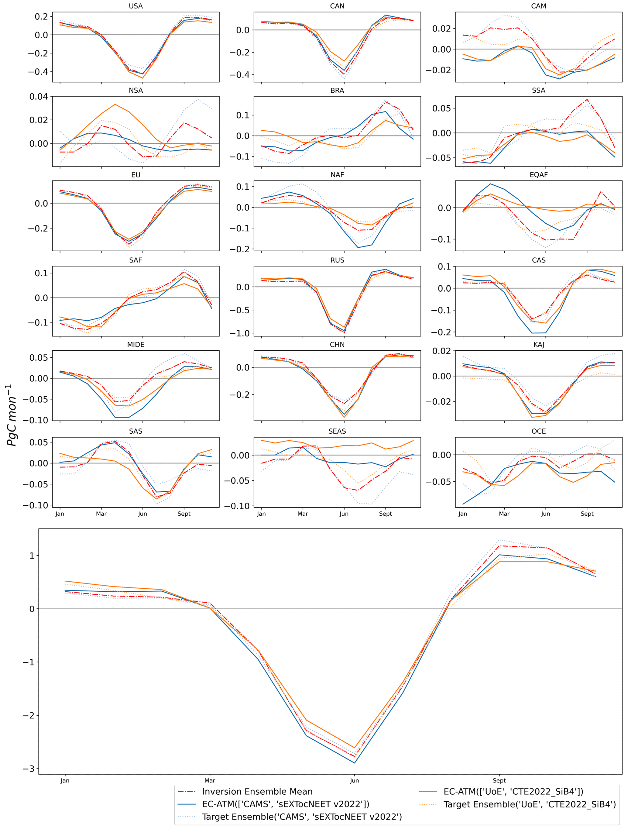
Figure C4 The MSC results for the “one-against-many” training runs, with EC-ATM models optimized against two inversion systems. The solid lines are the EC-ATM models trained using the named pair of inversion systems, and the dotted lines are MSC of the named pair's mean regional and global integrals. For all panels, the x axis is the yearly cycle, while the y axis is Pg C per month.

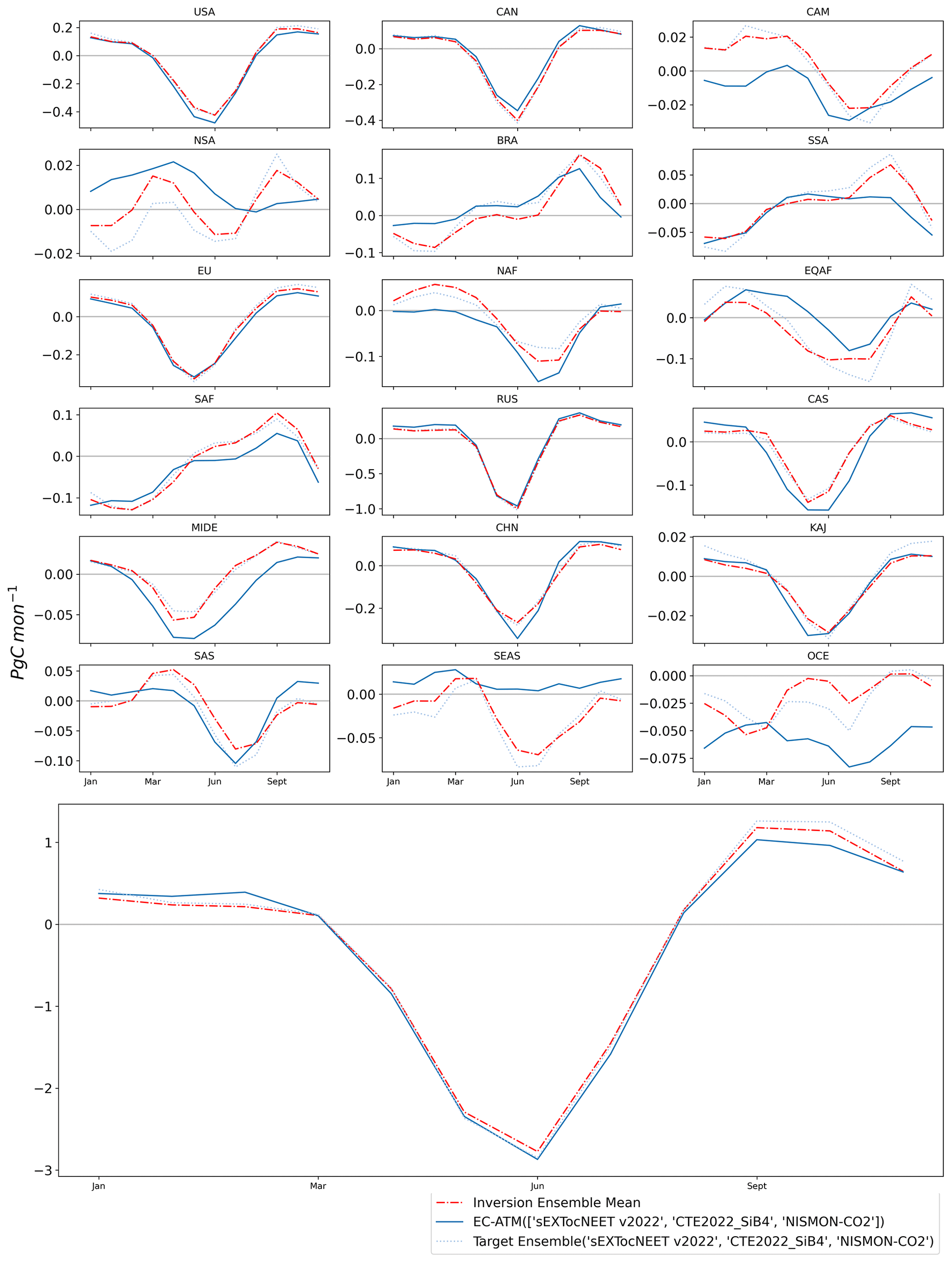
Figure C5 The MSC results for the “one-against-many” training runs, with an EC-ATM model optimized against three inversion systems. The solid line is the EC-ATM model trained using the named set of inversion systems, and the dotted line is the MSC of the named set's mean regional and global integrals. For all panels, the x axis is the yearly cycle, while the y axis is Pg C per month.​​​​​​​