Evaluation of WRF-Chem-simulated meteorology and aerosols over northern India during the severe pollution episode of 2016

We use a state-of-the-art regional chemistry transport model (WRF-Chem v4.2.1) to simulate particulate air pollution over northern India during September–November 2016. This period includes a severe air pollution episode marked by exceedingly high levels of hourly PM_2.5 (particulate matter having an aerodynamic diameter ≤ 2.5 µm) during 30 October to 7 November, particularly over the wider Indo-Gangetic Plain (IGP). We provide a comprehensive evaluation of simulated seasonal meteorology (nudged by ERA5 reanalysis products) and aerosol chemistry (PM_2.5 and its black carbon (BC) component) using a range of ground-based, satellite and reanalysis products, with a focus on the November 2016 haze episode. We find the daily and diurnal features in simulated surface temperature show the best agreement followed by relative humidity, with the largest discrepancies being an overestimate of night-time wind speeds (up to 1.5 m s⁻¹) confirmed by both ground and radiosonde observations. Upper-air meteorology comparisons with radiosonde observations show excellent model skill in reproducing the vertical temperature gradient (r>0.9). We evaluate modelled PM_2.5 at 20 observation sites across the IGP including eight in Delhi and compare simulated aerosol optical depth (AOD) with data from four AERONET sites. We also compare our model aerosol results with MERRA-2 reanalysis aerosol fields and MODIS satellite AOD. We find that the model captures many features of the observed aerosol distributions but tends to overestimate PM_2.5 during September (by a factor of 2) due to too much dust, and underestimate peak PM_2.5 during the severe episode. Delhi experiences some of the highest daily mean PM_2.5 concentrations within the study region, with dominant components nitrate (∼25 %), dust (∼25 %), secondary organic aerosols (∼20 %) and ammonium (∼10 %). Modelled PM_2.5 and BC spatially correlate well with MERRA-2 products across the whole domain. High AOD at 550nm across the IGP is also well predicted by the model relative to MODIS satellite (r≥0.8) and ground-based AERONET observations (r≥0.7), except during September. Overall, the model realistically captures the seasonal and spatial variations of meteorology and ambient pollution over northern India. However, the observed underestimations in pollutant concentrations likely come from a combination of underestimated emissions, too much night-time dispersion, and some missing or poorly represented aerosol chemistry processes. Nevertheless, we find the model is sufficiently accurate to be a useful tool for exploring the sources and processes that control PM_2.5 levels during severe pollution episodes.

1 Introduction

Atmospheric particle pollution in India is a persistent environmental issue and a leading health risk factor for its 1.4 billion population (Pandey et al., 2021). In 2019, ambient air pollution was estimated to cause almost a million premature deaths in India (Pandey et al., 2021). The State of Global Air 2022 (HEI, 2022) reports that over 90 % of the Indian population resides in areas where the annual mean concentrations of PM_2.5 (particulate matter having an aerodynamic diameter smaller than 2.5 µm) exceed even the minimal interim target of 35 µg m⁻³ recommended by the World Health Organization air quality guidelines (WHO, 2021). The country is home to 18 of the 20 cities worldwide with the greatest rise in PM_2.5 pollution in the last decade (HEI, 2022). This upward trend in degraded air quality is projected to continue across South Asia under current policies, including more frequent high-pollution incidents over northern India (R. Kumar et al., 2018; Paulot et al., 2022). These trends have huge consequences for the future life expectancy of the 400 million residents of this region which is currently reported to be reduced by more than 9 years under the current pollution burden (Greenstone and Fan, 2020).

The Indo-Gangetic Plain (IGP) is situated south of the Himalayas and stretches from parts of Pakistan in the west, through north and east India and Nepal, to Bangladesh in the east. The IGP is a heavily populated region (home to over 40 % of the total Indian population) with many rural, suburban and urban clusters (Fig. 1a). It is characterized by intensive multi-cropping systems, rapid industrialization and a growing economy, which results in a heterogeneous mix of particle and gaseous pollutant emissions (Venkataraman et al., 2018; A. Kumar et al., 2020). The region is a global centre for poor air quality (Singh et al., 2017), underpinned by India being one of the largest emitters of anthropogenic aerosols in the world (Lu et al., 2011). The anthropogenic sources include vehicles, industry, the burning of crop waste and garbage, residential cooking, and mining. The emissions contributions are dominantly composed of nitrate and sulfate precursors and carbonaceous aerosols, driven by a rapid increase in demand for energy (Lu et al., 2011). Black carbon (BC) is fine particulate matter's light-absorbing component (Lack and Cappa, 2010) and is released during incomplete combustion of carbon-containing fossil fuels like coal, oil and gas and biofuels like wood, agricultural residues and forest fires. BC particles are short-term climate forcers with a net positive radiative forcing (Ramanathan et al., 2001; Bond et al., 2013; Wang et al., 2014). BC emissions from India are some of the highest globally and significantly impact the Indian summer monsoon, regional climate and human health (Ramanathan et al., 2001). Natural particle sources such as mineral dust also substantially influence the air quality over the IGP and broader northern India (Li et al., 2017). Additionally, air quality over the IGP region is greatly affected by the prevailing meteorology, topography and long-range transport of pollutants (Kaskaoutis et al., 2014; Kumar et al., 2014; Schnell et al., 2018; Ojha et al., 2020).

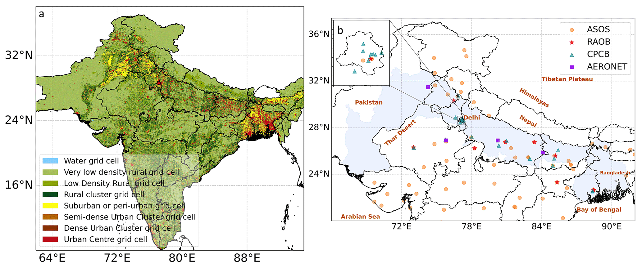
Figure 1 (a) Degree of urbanization based on 2015 human population size and built-up area density data over India from GHS-SMOD (Schiavina et al., 2022). (b) Locations of the observation sites used for comparison in this study; the legend indicates the different datasets (ASOS – automatic weather stations, RAOB – radiosonde observations, CPCB – Indian Central Pollution Control Board PM_2.5 ground monitoring stations, AERONET – Aerosol Robotic Network ground remote sensing observations). The inset figure is an enlarged map of Delhi capital, and the geographical area falling under the IGP region is highlighted in light blue.

In addition to the year-round poor air quality over the IGP region, recurring intense post-monsoon and winter haze episodes have been reported in numerous studies (Ram et al., 2016; M. Kumar et al., 2018; Kanawade et al., 2020; Beig et al., 2019; Bharali et al., 2019; Thomas et al., 2019; Dhaka et al., 2020; Kumari et al., 2021; Gupta et al., 2022). Most of these severe episodes coincide with the biomass burning period (mid-October to November), during which agricultural land is cleared in open fields by burning crop residue, primarily paddy (Singh et al., 2020). Although highly seasonal, the emissions from these multiple small to large fires emit large amounts of reactive gases and particles such as carbon monoxide (CO), nitrogen oxides (NO_x), volatile organic compounds (VOCs), carbonaceous particles and other components of PM_2.5 (Singh et al., 2020; Kumar et al., 2021). One such severe haze event over northern India occurred between 30 October and 7 November 2016, leading to daily mean PM_2.5 concentrations of 300–600 µg m⁻³, some 20–40 times greater than the 24 h WHO (2021) air quality guideline of 15 µg m⁻³ (Mukherjee et al., 2018; Sawlani et al., 2019; Kanawade et al., 2020; Jethva et al., 2019). Jethva et al. (2019) reported that crop residue fire counts over north-west India were particularly high in the 2016 post-monsoon period. Alongside crop biomass burning emissions, the unfavourable meteorology and accumulation of local urban emissions contributed to this week-long episode of extremely high pollution (Kanawade et al., 2020; Sawlani et al., 2019).

Modelling studies characterizing air pollution over India have utilized a variety of regional chemistry transport models (Nair et al., 2012; Kumar et al., 2012a, b; Moorthy et al., 2013; Pan et al., 2015; Srivastava et al., 2016; Schnell et al., 2018; Ghosh et al., 2023). These studies highlight various problems in simulating atmospheric composition over the Indian subcontinent, such as capturing the high aerosol loading, erroneous boundary-layer parameterizations, underestimations in emissions inventories, complex mountain topography and inaccurate moisture transport. This is especially true for simulations of surface BC concentrations, which utilize regional South Asian emissions inventories that are thought to underestimate the BC emissions (Kumar et al., 2015; Govardhan et al., 2019). Equally important is simulating the vertical distribution of BC particles and understanding their effect on atmospheric stability, for which only limited measurements have been made over India. These studies found high BC loadings vertically (up to 8 km altitude) over north-west and central India during different months (Babu et al., 2011; Bisht et al., 2016; Brooks et al., 2019). The role of these absorbing particles in modifying the vertical boundary layer structure during a haze episode over the northern Indian region has been poorly explored to date (Bharali et al., 2019).

This study aims to evaluate the WRF-Chem regional atmospheric chemistry transport model's ability to simulate the meteorology and aerosol chemistry across north India and the IGP in September–November 2016. Our choice to analyse the 2016 seasonality and the pollution episode differs from the previous literature (R. Kumar et al., 2020; Jena et al., 2020; Sengupta et al., 2022; Govardhan et al., 2023b) in several aspects, listed below.

• i.

  We use an updated WRF-Chem version (v4.2.1) and utilize the MOZART-MOSAIC chemical scheme (detailed in Sect. 2.1), which explicitly resolves the aerosols into four size bins and represents the chemistry of secondary organic and inorganic aerosols that make up the dominant components of PM_2.5 in the post-monsoon season, as compared to the GOCART scheme employed in these earlier studies which lacks particle size information.

• ii.

  The 2016 pollution episode over the IGP was one of the worst for air quality (since 2004) and anomalous for the highest rice crop production (since 2002) in NW Indian states, resulting in high crop residue burning in that year (Voiland and Jethva, 2017; Jethva et al., 2019; Sembhi et al., 2020). As shown by multiple trend analyses, 2016 had the highest number of agricultural fires of the last decade during the post-monsoon season (Sarkar et al., 2018; Mukherjee et al., 2018; Thomas et al., 2019; Kulkarni et al., 2020; Sembhi et al., 2020; Liu et al., 2021; Jethva, 2022; Gupta et al., 2023). Moreover, although several modelling studies have analysed the air quality during intense post-monsoon pollution episodes in the years after 2016 (e.g. Dekker et al., 2019; Beig et al., 2019; Kulkarni et al., 2020; Roozitalab et al., 2021), studies for 2016 are fewer (Sembhi et al., 2020; Mukherjee et al., 2020). It is, therefore, necessary to understand the implications of this particularly extreme episode with a chemistry transport model whose performance at simulating prevailing seasonal meteorology over a sufficiently long period has been evaluated.

• iii.

  The use of hourly fifth-generation European Centre for Medium-Range Weather Forecasts (ECMWF) reanalysis (ERA5) data to drive the model meteorology and a comprehensive comparison of the simulated meteorology and biases across northern India are an additional novelty of this work, as is the use of a wide range of ground and satellite observations as well as reanalysis products in the evaluation.

We first evaluate WRF-Chem simulations of surface and vertical meteorology against multiple available observations from weather stations and radiosonde profiles and reanalysis datasets. We then evaluate the modelled chemistry and aerosol optical properties against ground-based measurements, reanalysis products and satellite-retrieved data. The study focuses on characterizing monsoon to post-monsoon changes in meteorology and the atmospheric chemical composition of modelled PM_2.5 and BC in 2016.

2 Data and methods

2.1 WRF-Chem model description and configuration

The Weather Research and Forecasting model (version 4.2.1) coupled with Chemistry (WRF-Chem) (Grell et al., 2005; Fast et al., 2006) is an atmospheric chemistry transport model widely applied to the South Asia region, including its development as an air quality early-warning system for Delhi (Jena et al., 2021; R. Kumar et al., 2020). It has a terrain-following vertical coordinate system and is available with a range of physical parameterizations (Skamarock and Klemp, 2008). The transport of trace gases and aerosol species in WRF-Chem uses identical vertical and horizontal coordinates, allowing for feedback between meteorology and chemistry via radiation and photolysis (Grell et al., 2005). This makes WRF-Chem well-suited for investigating and isolating the interactions between aerosols and meteorology.

The single domain for this study covers the northern part of South Asia (20–38^∘ N, 66–90^∘ E) at 12 km horizontal resolution (Fig. 1b), with 33 vertical levels from the surface to the model top which is fixed at 50 hPa. The lowest 10 levels are below 1 km. The configurations of WRF-Chem dynamical and chemical parameterizations used in this study are adopted from the literature available for South Asia and are summarized in Table S1 in the Supplement. ERA5 data at a horizontal resolution of $\mathrm{0.25}{}^{\circ }\times \mathrm{0.25}{}^{\circ }$ are used for initializing the meteorology, boundary conditions and nudging in the model (Hersbach et al., 2020). Temperature, winds and water vapour are nudged towards ERA5 values above the planetary boundary layer (PBL) every 6 h, using grid nudging with a nudging coefficient of $\mathrm{6}\times {\mathrm{10}}^{-\mathrm{4}}$ s⁻¹ (Stauffer and Seaman, 1994). Terrestrial and land-use data are static and obtained from the MODIS IGBP 21-category land-cover classification (Friedl et al., 2002).

Time-varying boundary conditions for chemistry are taken from simulations of the global 6-hourly Model for Ozone and Related Chemical Tracers (MOZART-4)/Goddard Earth Observing System Model version 5 (GEOS-5) (NCAR, 2016). The simulation of gas-phase chemistry in WRF-Chem is provided by the updated MOZART-4 scheme (Emmons et al., 2010, 2020), which includes treatment of biogenic hydrocarbons and aromatics (Hodzic and Jimenez, 2011; Knote et al., 2014). Aerosol chemistry is simulated using the Model for Simulating Aerosol Interactions and Chemistry (MOSAIC) four-bin scheme (Zaveri et al., 2008). MOSAIC includes detailed solid-, liquid- and mixed-phase equilibria and thermodynamic gas–particle partitioning to compute aerosol composition and a simple parameterization of secondary organic aerosol (SOA) aqueous chemistry using glyoxal (Knote et al., 2014) but does not explicitly include detailed aqueous-phase chemistry, such as that described in Acharja et al. (2023). The aerosol processes in the mechanism include aerosol transport, dry and wet removal, water uptake, nucleation, coagulation, and condensation processes. The MOSAIC scheme uses a sectional approach to divide dry aerosol diameter into four discrete bins: 0.039–0.156, 0.156–0.625, 0.625–2.5 and 2.5–10 µm (the coarse-PM bin) (Zaveri et al., 2008). The aerosol distribution scheme includes both in-cloud and impaction scavenging and assumes aerosols to be internally mixed within the same bin and externally mixed between the bins (Riemer et al., 2019). MOSAIC simulates sulfate (SO${}_{\mathrm{4}}^{\mathrm{2}-}$), nitrate (NO${}_{\mathrm{3}}^{-}$), ammonium (NH${}_{\mathrm{4}}^{+}$), calcium (Ca²⁺), carbonate (CO${}_{\mathrm{3}}^{\mathrm{2}-}$), black carbon (BC), primary organic mass (OM), liquid water (H₂O), sea salt (NaCl) and other inorganic species such as minerals and trace metals (Zaveri et al., 2008). The Fast Tropospheric Ultraviolet–Visible (FTUV) photolysis scheme (Tie et al., 2003) provides photolysis rates and accounts for the aerosol feedback on photolysis (Hodzic and Knote, 2014).

Monthly anthropogenic emissions at $\mathrm{0.1}{}^{\circ }\times \mathrm{0.1}{}^{\circ }$ horizontal resolution are obtained from the 2010 Emission Database for Global Atmospheric Research for Hemispheric Transport of Air Pollution version 2.2 (EDGAR-HTAPv2.2; https://edgar.jrc.ec.europa.eu/dataset_htap_v2, last access: 13 February 2024). The emission sectors included in EDGAR-HTAPv2.2 are industrial, residential, transportation, agriculture, shipping, energy and aviation. For emissions from India, EDGAR-HTAPv2.2 incorporates the regional emissions inventory from the Model Inter-Comparison Study for Asia Phase III (MICS-Asia III) to derive emissions maps at a common grid resolution of $\mathrm{0.1}{}^{\circ }\times \mathrm{0.1}{}^{\circ }$ (Janssens-Maenhout et al., 2015). Within MICS-Asia III, a mosaic of regional anthropogenic emission inventories was developed by combining the nationally reported estimates by Argonne National Laboratory (ANL-India) and REAS2 (Regional Emission inventory in Asia) (Lu et al., 2011; Li et al., 2017). The total emissions for SO₂, NO_x, NH₃, PM₁₀, PM_2.5, BC, organic carbon (OC) and non-methane volatile organic compounds (NMVOCs) are speciated in the model following the MOSAIC-MOZART chemistry mechanism. The anthropogenic emissions exhibit a diurnal variation, with a simple transition between daytime and night-time values at 05:30 and 17:30 LT (local time) for each emitted pollutant, as specified by the preprocessor tool anthro_emis utility in the model (https://www2.acom.ucar.edu/wrf-chem/wrf-chem-tools-community, last access: 13 February 2024). The use of the 2010 EDGAR-HTAPv2.2 inventory to model air quality during 2016 adds some uncertainties to the model results as the emissions over India evolved from 2010 to 2016. Emissions of OC, CO, NO_x, SO₂ and NMVOCs from anthropogenic sectors such as industrial and energy sectors increased because of rapidly increasing demand, whilst primary particulate emissions of BC, OC and PM_2.5 from residential and informal industry sectors reduced due to cleaner fuel policies (such as the Ujjawala scheme; http://www.pmujjwalayojana.in/, last access: 13 February 2024) (McDuffie et al., 2020). The estimates derived from the global CEDS inventory reported by McDuffie et al. (2020) show a combined increase from road transport, energy, industry and agricultural sectors in annual NH₃, SO₂, NO_x and NMVOC emissions over India between 2010 and 2016. The reported increases in emissions of these pollutants across India are ∼17 %, ∼11 %, ∼12 % and ∼10 %, respectively. These changes in emissions may mean our model simulations underestimate the BC, primary OC and secondary aerosol contributions to total PM. However, it is challenging to fully isolate the impact of these changes in an atmospheric chemistry model because the model output also depends substantially on other factors, such as the meteorology, which drives online emissions. Compared with other global inventories of coarser resolution (e.g. ECLIPSE), the use of EDGAR-HTAPv2.2 has been found to simulate air quality over India with a greater local heterogeneity and to show slightly smaller overall biases when compared against reanalysis and satellite products (e.g. Upadhyay et al., 2020). Hence, although the EDGAR-HTAPv2.2 emissions are from 2010, we believe that they have been widely evaluated and are amongst the best available for our simulations.

In India, the post-harvest agricultural residue is largely cleared by burning it in open fields, and this is a dominant contributor to Indian PM_2.5, BC, OC, SO₂, NO_x and NMVOC emissions (Venkataraman et al., 2018). As EDGAR emissions do not include any biomass burning emissions (from agricultural fires, wildfires or prescribed fires), these are derived from the Fire Inventory from NCAR, version 1.5 (FINNv1.5) (Wiedinmyer et al., 2011). The emissions are based on satellite-measured locations of active fires and emission factors relevant to the underlying land cover (Akagi et al., 2011). The FINNv1.5 fire emissions inputs are distributed at 1 km spatial and hourly temporal resolution for 2016 (https://www.acom.ucar.edu/Data/fire/, last access: 13 February 2024).

Biogenic emissions are calculated online (updated every 30 min) using the Model of Emissions of Gases and Aerosol from Nature (MEGAN v2.0) (Guenther et al., 2006). MEGAN uses satellite-driven land-cover and modelled meteorological information (e.g. temperature and photosynthetically available radiation, PAR) to estimate VOCs, NO_x and CO from vegetation at spatial resolution. Dust emissions are generated online by incorporating the Goddard Global Ozone Chemistry Aerosol Radiation and Transport (GOCART) scheme from terrain data and modelled meteorology (Chin et al., 2002). The GOCART scheme, described in detail elsewhere (Ginoux et al., 2001; Zhao et al., 2010, 2013), utilizes the information about 10 m wind speed, threshold wind velocity (minimum value to reach for the dust emission to occur) and potential dust source region factors to calculate the dust emission flux. The total dust emission fluxes are calculated by multiplication by an empirical dimensional constant, which is taken from Ginoux et al. (2001). The GOCART scheme then distributes the emitted dust particles into four size bins (described earlier).

For our evaluation of WRF-Chem performance, hourly simulations are conducted for 1 September to 30 November 2016, allowing 6 d of spin-up (from 25–30 August). September falls within the south-west (SW) monsoon season (its withdrawal typically begins in mid-September), whilst October and November are in the post-monsoon season (India Meteorological Department, 2017). This permits a comparative assessment of meteorology and air quality between the two seasons. Although 2015–2016 was widely recorded as subject to a pronounced El Niño event, its effects over India only lasted until the summer of 2016 (India Meteorological Department, 2017) and therefore should not significantly impact the study period. In terms of general climatology, the 2016 SW monsoon rainfall was recorded to be normal over the country, aside from a deficit in rainfall over parts of north-west India.

2.2 Meteorological data

WRF-Chem-simulated meteorology is compared with observational networks measuring daily surface weather (Iowa Environmental Mesonet-Automated Surface Observing System; IEM-ASOS network) and atmospheric soundings (radiosonde observations (RAOB), University of Wyoming). Figure 1b shows the locations of the observation sites from these networks. The data links and access details are given in Table S2.

The IEM-ASOS network is an archive of global automated airport weather observations from weather stations operated by national agencies and airport authorities. Hourly 2 m air temperature (T2), relative humidity (RH), wind speed (WS) and wind direction (WD) data for 49 observation sites (Table S4) within the study domain are used. Processing and general quality control of the data are undertaken by the IEM network so the downloaded data were only checked for missing values before comparison with model output.

Radiosonde measurements for vertical meteorology profile comparison are available for eight sites within the model domain. Pilot balloon soundings are undertaken by the India Meteorological Department, and rigorous quality checks are performed before making them freely available (Durre et al., 2006). The radiosonde measurements are available each day at 00:00 UTC (05:30 and 17:30 IST (Indian standard time), respectively). No station has complete soundings for the entire study period, so model-measurement comparisons only include times when observations are available. The sounding observations are vertically interpolated to the model's pressure levels from 1000 to 100 hPa. The average vertical temperature, virtual potential temperature (VPT), WS and RH profiles are compared for individual sites, and temporal variability (as standard deviation) is reported for the entire period across all the pressure levels.

The spatial features of modelled meteorology are compared against the global MERRA-2 reanalysis (Gelaro et al., 2017) dataset available at a latitude–longitude grid resolution of $\mathrm{0.5}{}^{\circ }\times \mathrm{0.625}{}^{\circ }$ and 72-hybrid-eta levels at 6 h frequency. MERRA-2 reanalysis data are provided by NASA's Global Modelling and Assimilation Office (GMAO). The meteorological variables are re-gridded to WRF-Chem spatial resolution (12 km), and comparison was undertaken for T2, 10 m WS, water vapour mixing ratio (QV) and planetary boundary layer height (PBLH) variables.

2.3 Ground-based PM_2.5

We evaluate the performance of WRF-Chem in simulating aerosols by comparing modelled PM_2.5 mass concentrations and aerosol optical depth (AOD) at 550 nm with observations and reanalysis products. The measurements of surface PM_2.5 used for model comparison are undertaken by the Central Pollution Control Board of India (CPCB), accessed via the OpenAQ platform (Table S1, Fig. 1b). In addition to general quality control procedures applied by CPCB, the hourly PM_2.5 mass concentration data for 20 stations in the study domain were filtered for missing, zero and negative values. Days with <40 % of hourly measurements were also removed before comparing with the modelled PM_2.5 mass concentrations. Since Delhi has many more individual sites than other states in the domain, the data are grouped into two categories: all sites within the Delhi region (n=8) and the remaining sites (referred to as “Others”, n=12), the majority of which are located within the IGP region (Fig. 1b, Table S4).

2.4 Reanalysis PM_2.5 and black carbon concentrations

The spatial distributions of modelled surface PM_2.5 and BC concentrations are compared with MERRA-2 global reanalysis products, which are based on the GOCART scheme employed in GEOS-5 atmospheric model (Randles et al., 2017). The GOCART model in MERRA-2 employs the online coupling of radiatively active aerosols with meteorology in the GEOS-5 model. GOCART in MERRA-2 simulates OC, BC, sea salt, dust and sulfate aerosols, which are used to derive the total PM_2.5 mass concentrations, but it lacks information on size distribution and composition of aerosols. Additionally, the aerosols in the GOCART scheme are externally mixed and exclude the treatment of nitrate and secondary organic aerosols (Randles et al., 2017) due to which the MERRA-2 PM_2.5 is underestimated during high-pollution events (Buchard et al., 2017). Whilst the MERRA-2 AOD is directly constrained by the assimilation of observations, the aerosol diagnostics (such as PM_2.5) also partly depend upon systematic biases and assumptions of aerosol speciation and optical properties in the GEOS-5/GOCART model used in MERRA-2, as noted by Buchard et al. (2017). This is likely to influence the total PM_2.5 comparisons between WRF-Chem and MERRA-2, as WRF-Chem simulates a wider range of aerosol species. However, the utilization of MERRA-2 reanalysis data still serves as a useful reference for assessment of spatial and seasonal trends of aerosols between the two modelled datasets. AOD in MERRA-2 is assimilated using multiple satellite and ground-based observation data, including bias-corrected AOD from the Moderate Resolution Imaging Spectroradiometer (MODIS), Advanced Very High-Resolution Radiometer (AVHRR) instruments, Multi-angle Imaging Spectroradiometer (MISR) and Aerosol Robotic Network (AERONET). The aerosol assimilation uses satellite radiance and albedo from observing sensors and bias-corrected AOD, described in detail in Randles et al. (2017). Based on past studies and recommendations, the PM_2.5 concentration from MERRA-2-produced aerosol fields is calculated via the following summation of aerosol components in the size bin ≤ 2.5 µm diameter.

$$\begin{array}{}\text{(1)}& \begin{array}{rl}\left[{\mathrm{PM}}_{\mathrm{2.5}}\right]& =\left[\mathrm{BC}\right]+\mathrm{1.6}\times \left[\mathrm{OC}\right]+\mathrm{1.375}\times \left[{\mathrm{SO}}_{\mathrm{4}}^{\mathrm{2}-}\right]\\ & +\left[\mathrm{dust}\right]+\left[\mathrm{sea}\mathrm{salt}\right]\end{array}\end{array}$$

The multiplication factor of 1.375 on the sulfate ion concentration is based on the assumption in MERRA-2 that sulfate is primarily present as neutralized ammonium sulfate (Buchard et al., 2016; Provencal et al., 2017; Song et al., 2018). OC in MERRA-2 is scaled up to organic matter concentration using values ranging from 1.2–2.6, and this study uses the factor 1.6, which is commonly used for urban carbonaceous particles (Chow et al., 2015; Buchard et al., 2016; Provencal et al., 2017; Song et al., 2018).

2.5 Satellite and ground-based AOD data

WRF-Chem AOD at 550 nm is compared with satellite observations from the MODIS sensor on board the Terra and Aqua polar orbiting satellites. The AOD products from MODIS have a 10 km horizontal resolution at equatorial local overpass times of 10.30 (Terra) and 13.30 (Aqua). AOD retrievals from MODIS are based on combined Dark Target (DT: retrieval algorithm over dark land and ocean surfaces) and Dark Blue algorithms (DB: bright land surface) and re-gridded to the WRF-Chem resolution of 12 km. AOD in WRF-Chem is simulated between wavelengths 300–1000 nm and interpolated to 550 nm using the Ångström power law (Ångström, 1964; Kumar et al., 2014). In addition, ground-based AERONET version 2 level 2.0 (quality-assured and cloud-screened) AOD is available at four locations (Fig. 1b) within the study domain and is used for comparison with modelled results. AERONET is a global network (Holben et al., 1998) that has been extensively used for validating satellite observations over South Asia (Sayer et al., 2014; Mhawish et al., 2017).

2.6 Statistical metrics

Statistical metrics used here for the evaluation of model performance include mean bias (MB), normalized mean bias (NMB), mean absolute error (MAE), root mean square error (RMSE) and Pearson's correlation coefficient (r). Definitions of these metrics are provided in Table S3.

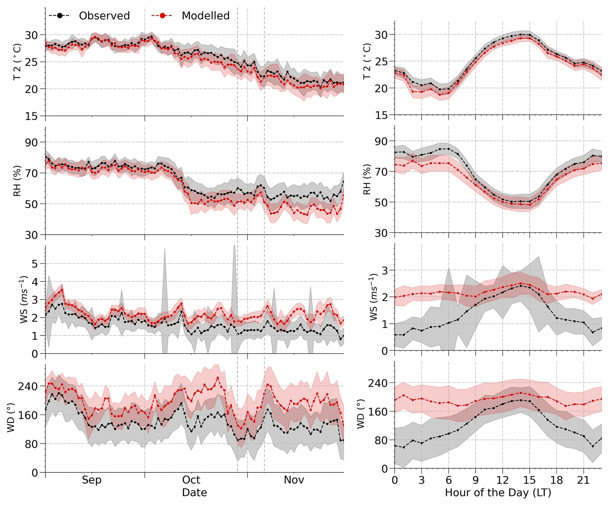
Figure 2 Daily-mean time series (left panels) and mean diurnal cycle (right panels) of observed (black) and modelled (red) meteorological variables from 1 September–30 November 2016 averaged across the 49 ASOS measurement sites shown in Fig. 1b. From top to bottom: daily mean 2 m temperature, relative humidity, wind speed and wind direction. The shaded regions indicate the standard deviation in the spatial variability in the model and measured variables. The vertical dashed lines delineate the period of severe high pollution between 30 October and 7 November.

3 Meteorology evaluation results

3.1 Near-surface meteorological fields

Figure 2 shows modelled and measured time series of daily means and mean diurnal cycles T2, RH, WS and WD derived from hourly data and averaged across all the observational sites. The statistical comparison metrics for the 3 months are provided in Table 1. As the exact measurement heights at individual sites are not known, the comparisons are made assuming the standard above-ground heights of 2 m for temperature and RH and 10 m for wind speed and direction. Daily average T2 variability correlates well between the model and observations for all the months (r>0.85), with maxima and minima captured well (Fig. 2). Model MB for T2 is slightly lower but by less than −0.8 ^∘C for all months. The T2 diurnal profile is also well represented by the model, with differences slightly larger (up to 2 ^∘C) during night-time.

Table 1 Summary of statistical comparison of modelled and observed meteorology variables derived from hourly data between September and November 2016 and averaged across the 49 ASOS measurement sites shown in Fig. 1b. The statistical metrics used for comparison are mean bias (MB), normalized mean bias (NMB), mean absolute error (MAE), root mean square error (RMSE) and Pearson's correlation coefficient (r).

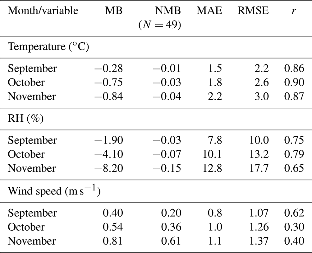
The general day-to-day variability in modelled surface RH also compares reasonably well with the observations (r range across the months: 0.65–0.79), with slight underestimations that gradually increase from −1.9 % in September to −8.2 % in November mainly due to underestimations seen in the night-time RH peaks. The observed diurnal RH cycle is also well simulated by the model although as for T2 with larger differences during the night when RH is greatest.

The differences in simulated 10 m wind patterns are relatively higher than those for T2 and RH, with modelled WS showing a relatively poor correlation of r≤0.4 and overestimations of about 0.5–0.8 m s⁻¹ (36 %–61 %) in October and November. However, better correlation (r=0.62) and lower biases (MB = 0.4 m s⁻¹ and NMB = 0.2) are observed for September. The diurnal variation of WS during daytime is captured quite well by the model, while the bias is higher at night (up to 1.5 m s⁻¹); this is the reason for the observed large biases in modelled daily variabilities in WS. Since local WD is highly variable across sites in different regions, it is hard for a model to capture the daily variabilities. Differences between modelled and observed WD are smallest during the daytime when the general wind direction is south-westerly and largest at night.

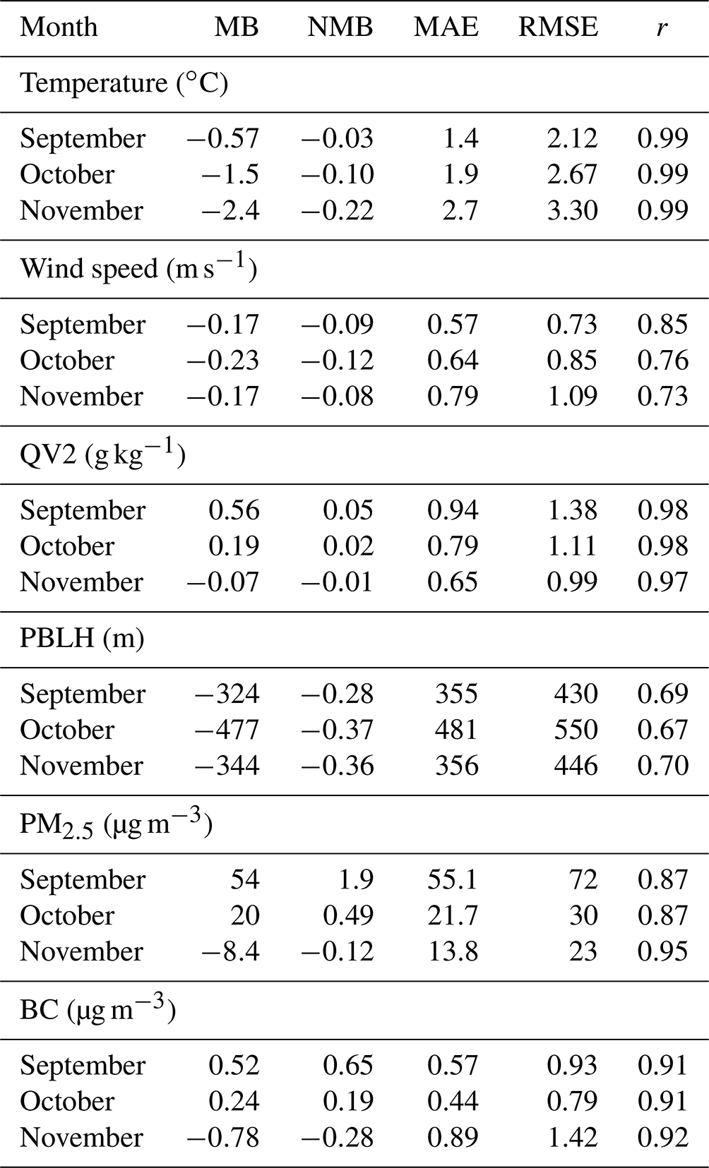
Table 2 provides the statistical evaluation results from the comparison of WRF-Chem and MERRA-2 global reanalysis data for mean T2, 10 m wind speed, water vapour mixing ratio (QV) and planetary boundary layer height (PBLH). The spatial maps of these variables are presented in Figs. S1 and S2 in the Supplement. Except for PBLH, the meteorological variables generally show good spatiotemporal agreement between the model and MERRA-2, with the best agreement for T2 and QV, as reflected in the high spatial correlations (r≥0.97). However, regional heterogeneities exist between the two datasets which are generally more evident temporally across all the variables. The largest spatial differences are seen for WS and QV, which show overall underestimations by WRF-Chem for WS (in contrast to observed overestimations as compared to the measured data) and overestimations for QV (in contrast to observed underestimations as compared to the measured data) in the wider IGP region. There is a stronger west–east gradient in PBLH in MERRA-2 compared to WRF-Chem which possibly influences the PM_2.5 concentrations in MERRA-2.

Table 2 Summary of statistical comparison of WRF-Chem- and MERRA-2-derived meteorology variables from September to November 2016. The statistical metrics used for comparison are mean bias (MB), normalized mean bias (NMB), mean absolute error (MAE), root mean square error (RMSE) and Pearson's correlation coefficient (r).

A seasonal dry bias in the WRF model over the Indian region due to possible errors in moisture fluxes has been reported previously (Kumar et al., 2012b; Conibear et al., 2018), and night-time underestimations in modelled RH similar in magnitude to this study were noted by Gunwani and Mohan (2017). A comparison of modelled results, including ERA5 (used to drive WRF-Chem here) and independent MERRA-2 global reanalysis datasets with hourly ground observations (Fig. S3), shows the highest positive bias in RH in ERA5 during all the months, while WRF-Chem and MERRA-2 tend to underestimate RH across all the months. This may affect the model's ability to capture the diurnal evolution of secondary aerosols by hygroscopic growth, particularly at night.

The observed positive bias in simulated 10 m WS (also seen in Fig. S1 meteorology comparison with ERA5 and MERRA-2) is well known, and the observed magnitude of the bias is largely consistent with previous studies (Zhang et al., 2016; Mues et al., 2018; Gunwani and Mohan, 2017; Wang et al., 2021). First, this could be in part due to inaccurate land-surface parameterizations (such as roughness length or surface drag and urban canopy), yielding smaller friction velocities and stronger winds in the model. Second, it could also be due to unknown differences in heights of measured and modelled WS. However, the afternoon-simulated WS levels are close to the observations, which suggests there are underlying weaknesses in nocturnal stable boundary layer decoupling in the model. The associated turbulent fluxes and thermodynamic exchanges occurring in the atmospheric boundary layer are important for model-simulated PBL and pollutant dispersal (Shen et al., 2023; Nelli et al., 2020). However, during the extreme-pollution episode (30 October to 7 November), both the model and observations agree on a reduction in WS (although with varying magnitudes) and a shift in WD. These changes highlight the role of stagnant meteorology in greatly enhancing the near-surface pollution lasting over a week.

3.2 Vertical profiles

Figures 3 and 4 show averaged modelled and observed sounding profiles over individual RAOB sites (Fig. 1) for temperature (T), virtual potential temperature (VPT) and wind speed (WS) at 05:30 IST (00:00 UTC) and 17:30 IST (12:00 UTC), respectively. The corresponding summaries of statistical metrics are presented in Tables 3 and 4. The upper-air meteorology and thermodynamic structure are crucial parameters of the atmosphere as they impact the transport and convective distribution of pollutants. Of all the meteorological quantities examined here, vertical profiles of T and VPT are represented best by the model, with correlations of r≥0.95 across all the sites and r=1.0 for most of the sites at both times. At 05:30 IST, modelled T profiles show a warm bias of up to 1.5 ^∘C at six sites and a cold bias of up to 2 ^∘C at Delhi and Gwalior sites up to about 980 hPa (Fig. 3a), which gradually decreases with altitude. The model also captures the observed marked inversion near the surface in morning T and VPT profiles reasonably well at most sites. Agreement at 17:30 IST is even better (Fig. 4a): biases in modelled T profiles are less than 0.5 ^∘C below 980 hPa at all sites except Ranchi and negligible aloft. Overall, across all sites, the average MB, NMB and RMSE values are generally lower for VPT compared to T at both times (Tables 3 and 4).

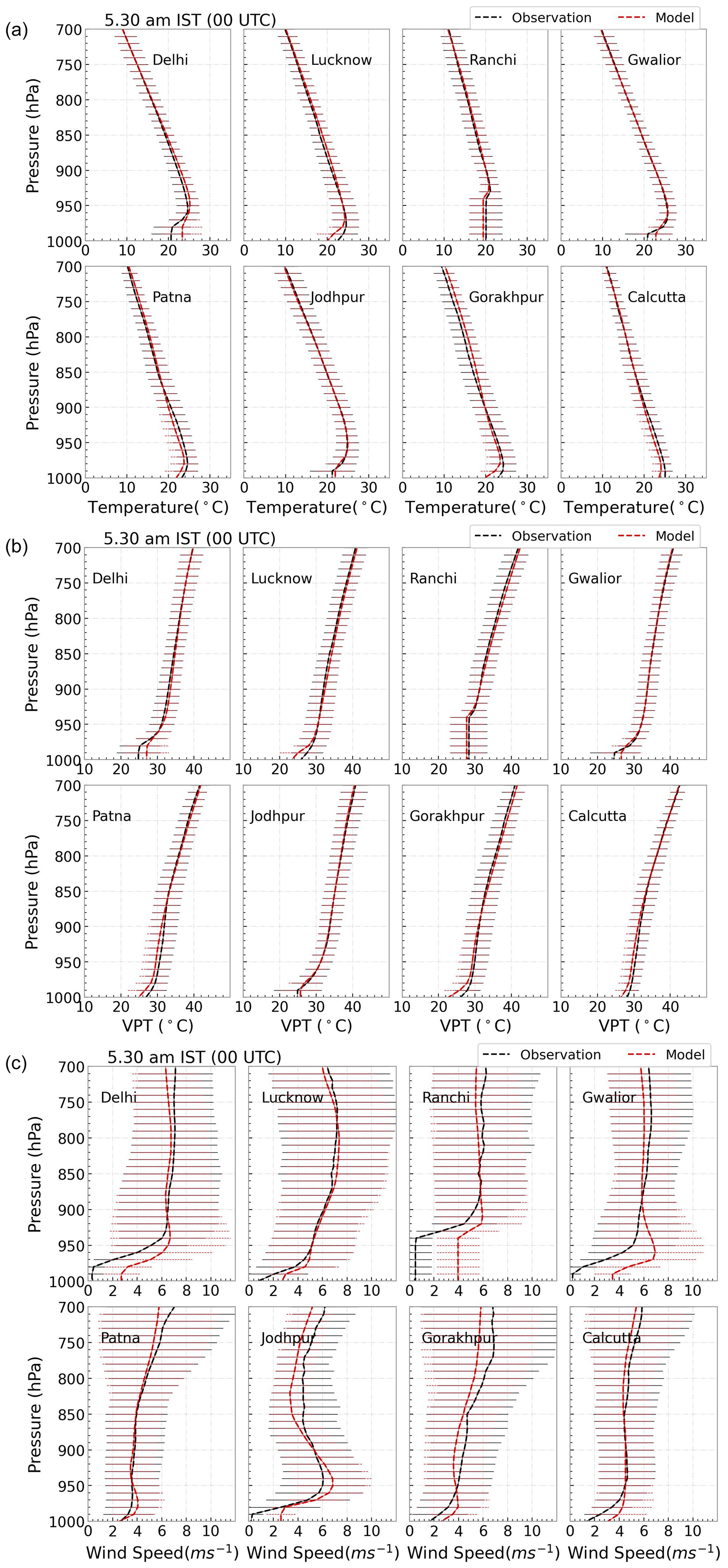
Figure 3 Top to bottom: comparisons of vertical profiles of temperature (^∘C), virtual potential temperature (VPT; ^∘C), and wind speed (m s⁻¹) between the model (red) and radiosonde observations (black) for eight sites at 00:00 UTC (05:30 IST) averaged for September–November 2016. The horizontal lines show the standard deviation in the day-to-day temporal variability during the comparison period.

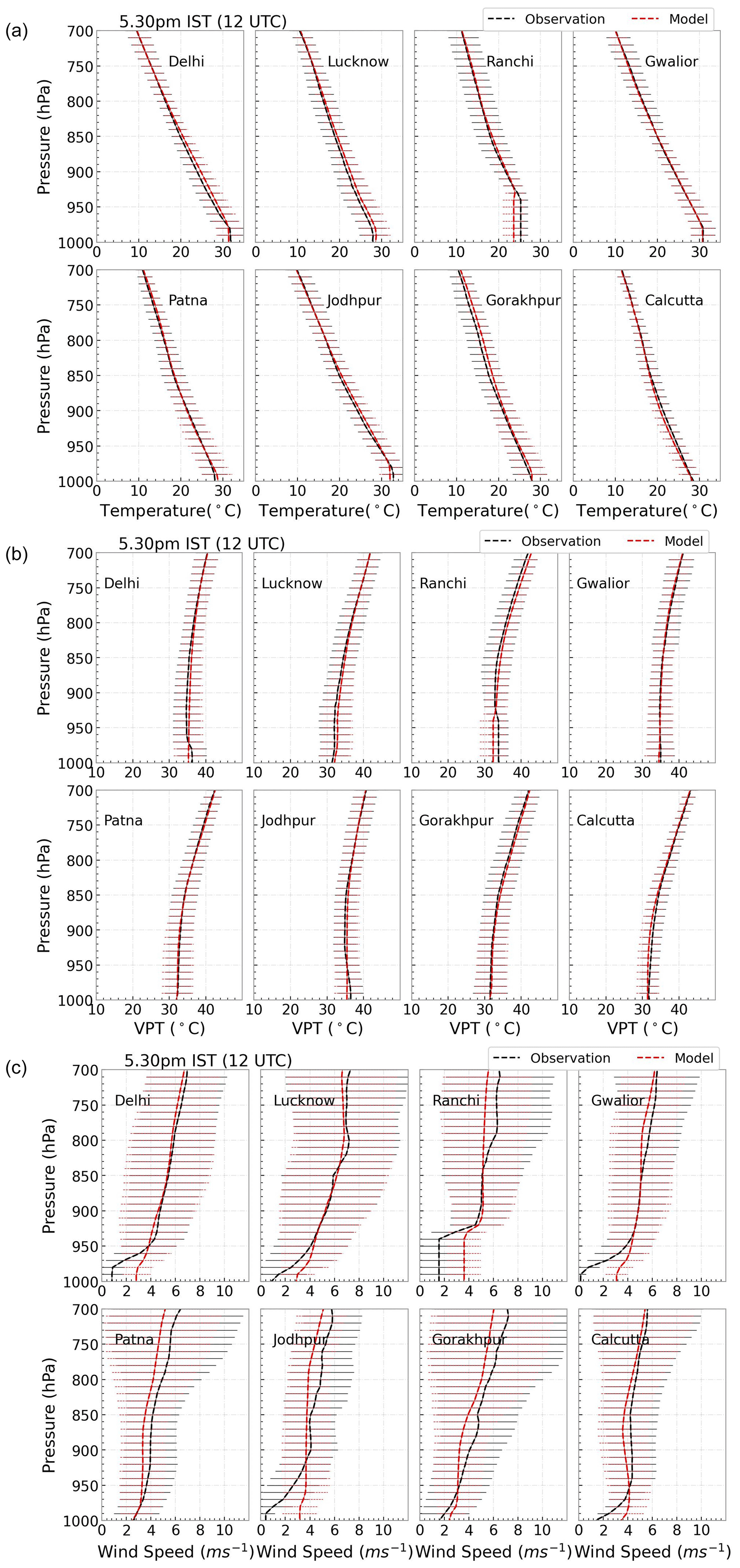
Figure 4 Top to bottom: comparisons of vertical profiles of temperature (^∘C), virtual potential temperature (VPT; ^∘C), and wind speed (m s⁻¹) between the model (red) and radiosonde observations (black) for eight sites at 12:00 UTC (17:30 IST) averaged for September–November 2016. The horizontal lines show the standard deviation in the day-to-day temporal variability during the comparison period.

Table 3 Summary of statistical comparison of modelled and observed 05:30 IST profiles derived from radiosonde data for the individual RAOB stations shown in Fig. 1b averaged from September to November 2016. The statistical metrics used for comparison are mean bias (MB), normalized mean bias (NMB), mean absolute error (MAE), root mean square error (RMSE) and Pearson's correlation coefficient (r).

Table 4 Same as Table 3 but for 17:30 IST profiles.

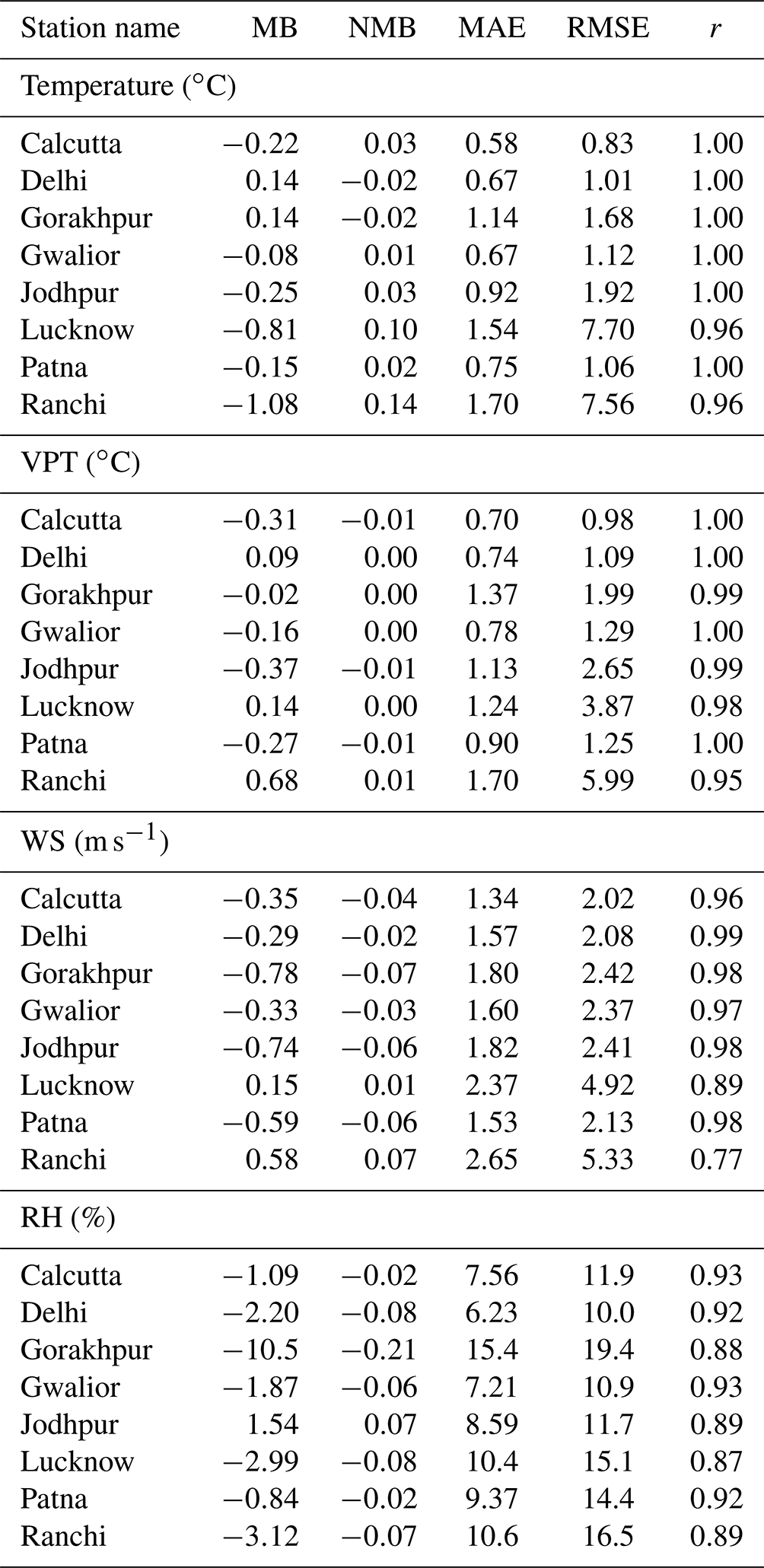
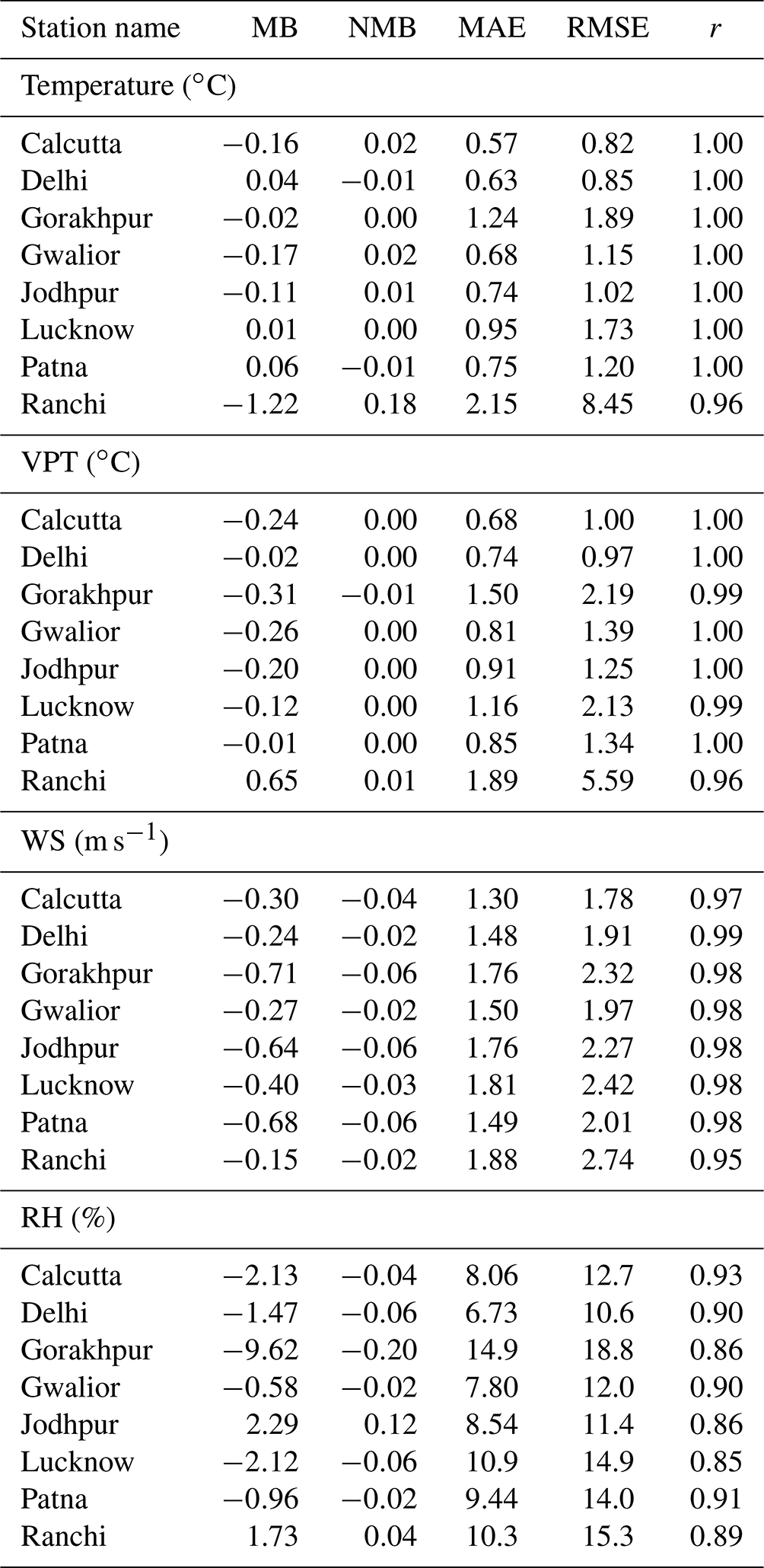
The simulated WS vertical profiles have larger variations across most of the sites at both times compared to T and VPT profiles (Figs. 3c and 4c). Consistent with the 10 m WS comparisons, the model tends to overestimate WS vertically by up to 4 m s⁻¹ at 05:30 IST and up to 3 m s⁻¹ at 17:30 IST in the lower layers but better captures it aloft (above ∼900 hPa), with only slight differences across all the sites (Fig. S4). Despite the considerable positive bias within the bottom layers, the model reproduces the observed higher WS at higher altitudes reasonably well, resulting in good correlations of r≥0.77 at 05:30 IST and r≥0.95 at 17:30 IST. As an exception, the modelled WS profiles are very well represented over the Patna site (in the east) during both times. The results here differ from those of Mohan and Bhati (2011), who noted increased deviation in simulated WS at higher altitudes over Delhi during the summer months.

The simulated RH profiles were also evaluated (Fig. S4) and show underestimations by up to 20 % in the lower layers of the model across most sites at both times, which decreases in magnitude at higher altitudes except at Gorakhpur. These biases vertically are generally more negative at 05:30 IST compared to 17:30 IST, indicating a dry bias in the early morning hours in the model, consistent with the ground observation comparisons.

VPT profiles are particularly useful in understanding the stability and turbulence of the atmosphere, which helps in the dilution of the pollutants within the mixed boundary layer. By accounting for moisture and temperature, a VPT profile indicates buoyancy and stability in the atmosphere and can be used to derive planetary boundary layer heights (Liu et al., 2019; Vogelezang and Holtslag, 1996). Figure 3 shows that, at all sites, observed and simulated temperature inversion layers are close to the surface at 05:30 IST, demonstrating the typical formation of an urban nocturnal stable boundary layer. In contrast, at 17:30 IST (Fig. 4), both the observed and modelled VPTs exhibit a typical well-mixed late-afternoon profile due to surface heating, with higher values of VPT near the surface (33–36 ^∘C surface) that remains nearly constant up to about 850 hPa across most sites. The negligible biases and error statistics in T and VPT profiles (Tables 3 and 4) across all sites provide high confidence in model skill in simulating the thermodynamic structure of the atmosphere. This is an improvement on Mues et al. (2018), who reported larger biases in T profiles (up to 3 and 7 ^∘C at 05:30 and 17:30 IST, respectively) at the Delhi site in winter and summer 2013. As noted in Sect. 3.1, and elsewhere (Mohan and Bhati, 2011; Gunwani and Mohan, 2017), errors in simulated WS are highly sensitive to local roughness length and model topography and are thus subject to greater noise. Given these limitations, we find the model performance statistics comparable to previous studies (Mohan and Bhati, 2011; Kumar et al., 2012b) and close to the benchmarks provided by Emery and Tai (2001).

4 Chemistry evaluation results

4.1 Ground-based PM_2.5

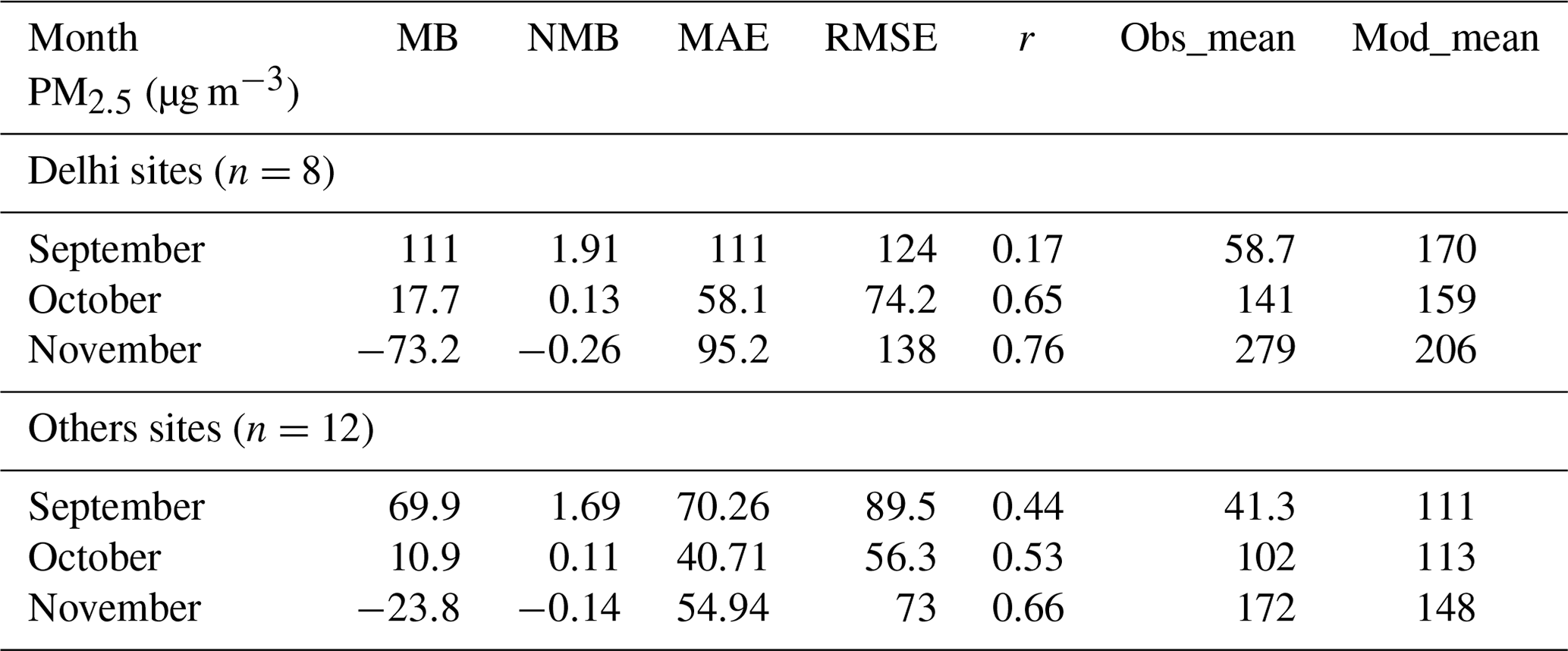
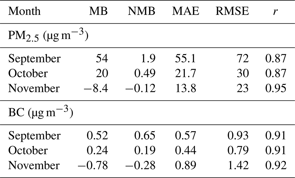
Figure 5 compares the modelled and measured daily averaged time series (left) and diurnal variability (right) of surface PM_2.5 concentrations from hourly samples from September to November 2016. The observations are spatially averaged across 8 sites in Delhi and 12 sites across the rest of the domain (referred to as “Others”). The statistical summary is presented in Table 5. The model adequately captures the day-to-day variation of PM_2.5 for October–November, when it is biased low, while it fails to reproduce the daily variability during September when it is strongly biased high. On average, during September, the model overestimates surface PM_2.5 concentrations by more than a factor of 2 (NMB range: 1.69 to 1.91) across all the sites and underestimates in November by 26 % over Delhi and by 14 % over Others. Overall, the model and observed daily surface PM_2.5 correlate reasonably well during October (Delhi – r=0.65, Others – r=0.53) and November (Delhi – r=0.76, Others – r=0.66). Correlation for these months is better across Delhi sites but shows relatively larger mean biases (+17.7 to −73.2 µg m⁻³) and NMBs (+0.13 to −0.26) compared to Others. Additionally, the model tends to predict PM_2.5 concentrations with a fairly broad range of monthly RMSE values (56.3–138 µg m⁻³).

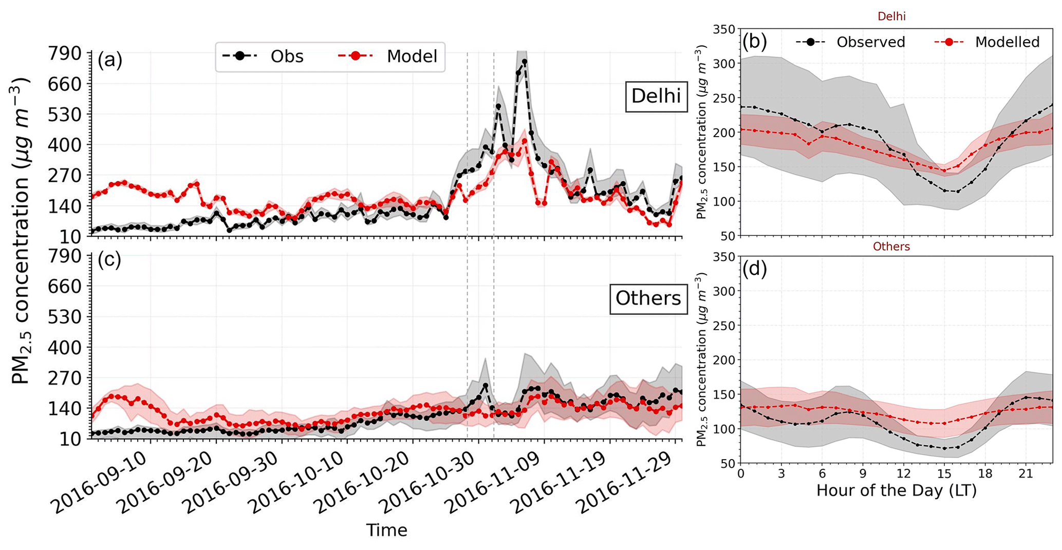
Figure 5 Time series of daily means (a, c) and mean diurnal cycles (b, d) of observed and modelled PM_2.5, averaged across 8 sites in Delhi and 12 sites over the rest of the domain (labelled “Others”) from September–November 2016. The shaded area in both panels shows standard deviation of the spatial variability of the model and measured PM_2.5. The locations of the ground measurement sites are shown in Fig. 1b. The vertical dashed lines delineate the period of severe high pollution between 30 October and 7 November.

Table 5 Statistical summary of comparisons of modelled and observed PM_2.5 concentrations derived from hourly data between September and November 2016 for Delhi (top) and Other stations (bottom). The statistical metrics are mean bias (MB), normalized mean bias (NMB), mean absolute error (MAE), root mean square error (RMSE) and Pearson's correlation coefficient (r). n denotes the number of available measurement stations in the group.

The spatially averaged diurnal cycle for modelled surface PM_2.5 shows a pronounced diurnal trend matching observations for Delhi sites, while the diurnal cycle is less pronounced at Others sites. Generally, diurnal trends are in good agreement across all sites, although on average, the model tends to underpredict the afternoon dips and night-time peaks compared to the observations, indicating missing anthropogenic activities from the simplified diurnal emissions patterns derived from monthly estimates used in the model. The lack of a representation of a realistic diurnal activity cycle in the anthropogenic emissions highlights that meteorology could be driving the modelled PM_2.5 variation. However, this might partly be affected by the imperfectly represented diurnal variability of WS in the model (Sect. 3.1).

During the 30 October–7 November pollution episode, both observations and the model show the highest daily mean surface PM_2.5 (observed – 300–750 µg m⁻³, modelled – 150–420 µg m⁻³) across Delhi, while relatively lower concentrations are seen across Others sites during this period (observed and modelled: <200 µg m⁻³) (Fig. 5). The observed daily mean PM_2.5 concentrations exceed the 24 h average 2021 WHO air quality guideline of 15 µg m⁻³ (WHO, 2021) by nearly 50 times, and the predicted concentrations are exceeded by nearly 28 times. The maximum negative differences (up to 350 µg m⁻³) between the daily mean modelled and observed PM_2.5 also occur during this episode. During this period, the observed hourly PM_2.5 concentrations exceed 1000 µg m⁻³ (mostly at night) at the Delhi US embassy site (in central Delhi) and exceed 800 µg m⁻³ at all the sites across Delhi and two downwind stations in the lower IGP (Lucknow and Kanpur). The corresponding modelled hourly concentrations at these locations and times underestimate PM_2.5 by a factor of 2–3 (380–520 µg m⁻³), in part attributable to overestimated surface WS.

One study characterizing this 2016 high-pollution episode over Delhi reported exceptionally high night-time mean PM_2.5 concentrations of 2924 µg m⁻³ on 30 October (Diwali festival night), 1520 µg m⁻³ on 5 November and daytime mean values of nearly 1500 µg m⁻³ on 6 November (Sawlani et al., 2019). The modelled and observed daily average PM_2.5 across downwind Others sites only peaks (>250 µg m⁻³) towards the end of the high-pollution episode, suggesting a regional distribution of PM_2.5 over time. The observed and simulated near-surface meteorology during this time over northern India shows stagnant conditions conducive to the build-up of pollutants: smaller WS (1–1.5 m s⁻¹), lower PBLH (<500 m) and a nearly 2–3 ^∘C drop in near-surface temperature, leading to atmospheric inversion (Fig. 2). These stagnant conditions combined with regional and local anthropogenic emissions facilitate pollution accumulation within the shallow continental boundary layer over wider northern India. After the extreme-pollution days (9 November onwards), the model captures the magnitude of daily PM_2.5 variation well everywhere except for an observed peak across Delhi on 17 November.

4.2 Modelled PM_2.5 composition

The daily time series and average diurnal variability of modelled mean surface PM_2.5 composition over observation sites in Delhi and Others are shown in Fig. 6. Due to the lack of observed PM_2.5 speciation data for this period, only modelled results are presented here. These are qualitatively compared with literature for other years as the aerosol loading over the Indian region exhibits stronger intra-annual variabilities than interannual variabilities (Conibear et al., 2018; Mhawish et al., 2021). The largest variations in daily PM_2.5 components across all months are observed for secondary organic aerosol (SOA) and secondary inorganic aerosol (SIA) (sulfate, nitrate and ammonium) over all the sites. The concentration of fine dust particles dominates most evidently at the beginning of September and reduces to almost half in October and November but remains a non-negligible contributor to total PM_2.5 on average (15 %–25 %) across all sites. The fine dust component is mainly responsible for the overestimations seen in modelled PM_2.5 in September compared to the measurement. Another notable change is in the nitrate component which dramatically peaks during the high-pollution period, together with SOA, ammonium and primary aerosols (OC, BC). The modelled peaks in PM_2.5 and its components largely follow the observed PM_2.5 trend (October–November period), which highlights the model's skill in representing the diversity of aerosols during dramatic shifts in surface particle pollution and is more clearly seen across Delhi sites than Others. Among SIA, the PM_2.5 composition in November is dominated by nitrate aerosols (10 %–30 %), which are comparable to reported measurements. For example, a high nitrate fraction (20 %–27 %) in post-monsoon months has been reported in various measurement studies over India (Ram and Sarin, 2011; Schnell et al., 2018; Patel et al., 2021; Talukdar et al., 2021). The average modelled BC contribution over Delhi during September (3 µg m⁻³), October (8.2 µg m⁻³) and November (13.2 µg m⁻³) is comparable to the measured elemental carbon (EC; assumed to be equivalent to modelled BC) concentrations (∼3, ∼6 and ∼12 µg m⁻³, respectively) reported by Sharma et al. (2018). The dominance of secondary particle contribution to modelled PM_2.5 during post-monsoon months is fully consistent with other studies (Gani et al., 2019; Talukdar et al., 2021), although the relative abundance is lower. The diurnal variation of PM_2.5 components over Delhi shows more pronounced dips in primary and secondary inorganics, suggesting the influence of local emissions, while the fine dust component remains relatively stable, suggesting both local and natural non-local emissions influence.

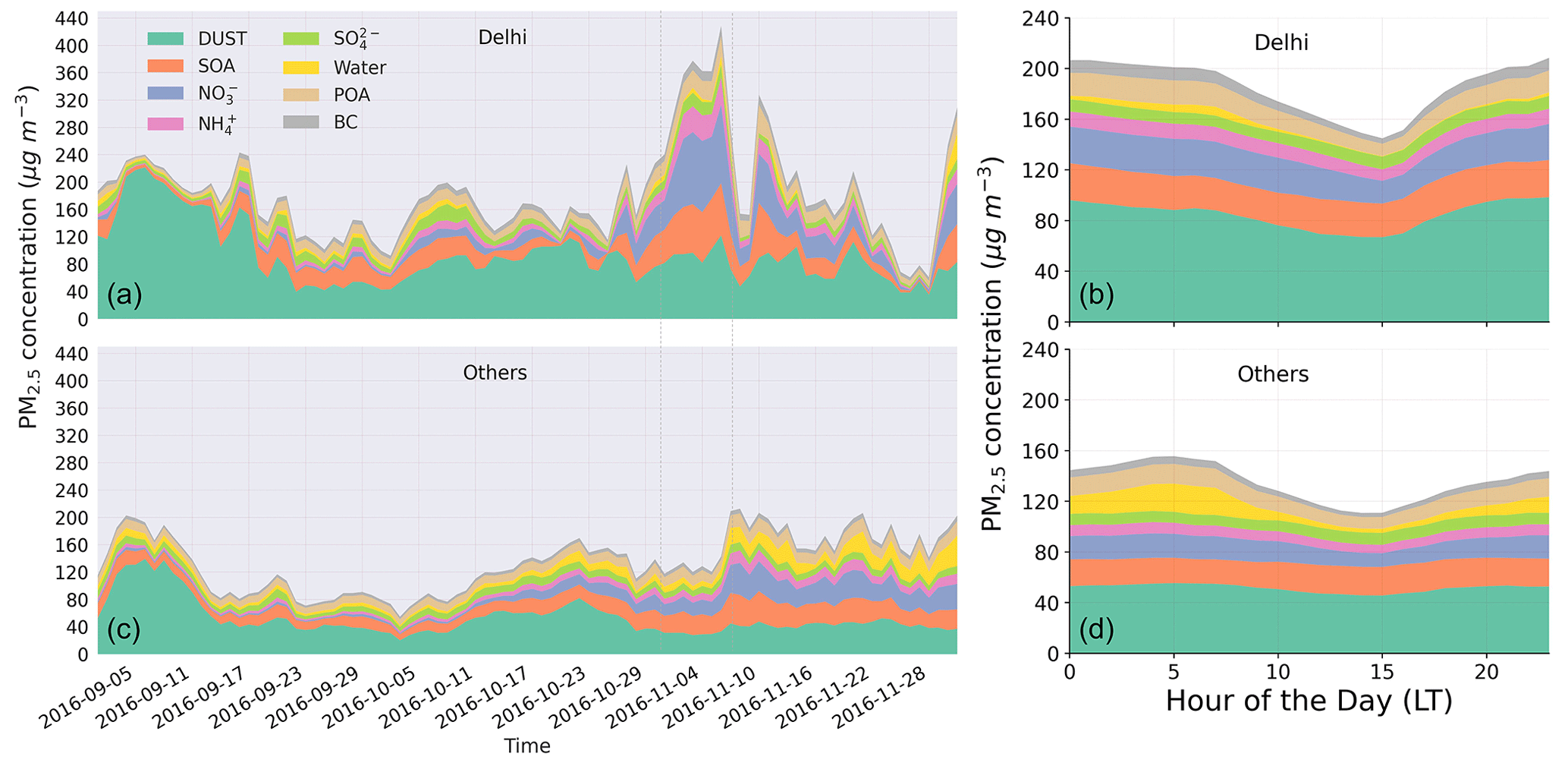
Figure 6 Time series of daily means (a, c) and mean diurnal cycles (b, d) of modelled individual PM_2.5 components averaged across 8 stations in Delhi and 12 stations over the rest of the domain (labelled “Others”) from September–November 2016. The individual species contribution abbreviations are as follows: SOA (secondary organic aerosol), POA (primary organic aerosol), SO${}_{\mathrm{4}}^{\mathrm{2}-}$ (sulfate), NH${}_{\mathrm{4}}^{+}$ (ammonium), NO${}_{\mathrm{3}}^{-}$ (nitrate) and BC (black carbon). The vertical dashed lines delineate the period of severe high pollution between 30 October and 7 November.

4.3 Comparison of PM_2.5 and black carbon distribution with reanalysis products

Figure 7 compares the monthly averaged spatial distribution of WRF-Chem-modelled and MERRA-2-reanalysis-derived surface PM_2.5 and BC concentrations. The corresponding domain-averaged performance statistics are summarized in Table 6. The overall spatial agreement between the model and MERRA-2 is excellent for both PM_2.5 and BC (r>0.87, Fig. S6). However, on a regional scale, the modelled PM_2.5 is biased high over parts of arid western India and eastern Pakistan in September, resulting in a domain-wide NMB of 1.9. The model shows a stronger west–east gradient in PM_2.5 than MERRA-2, with the highest modelled concentrations of >250 µg m⁻³ in the western and north-western regions. Agreement between the model and MERRA-2 improves for October–November.

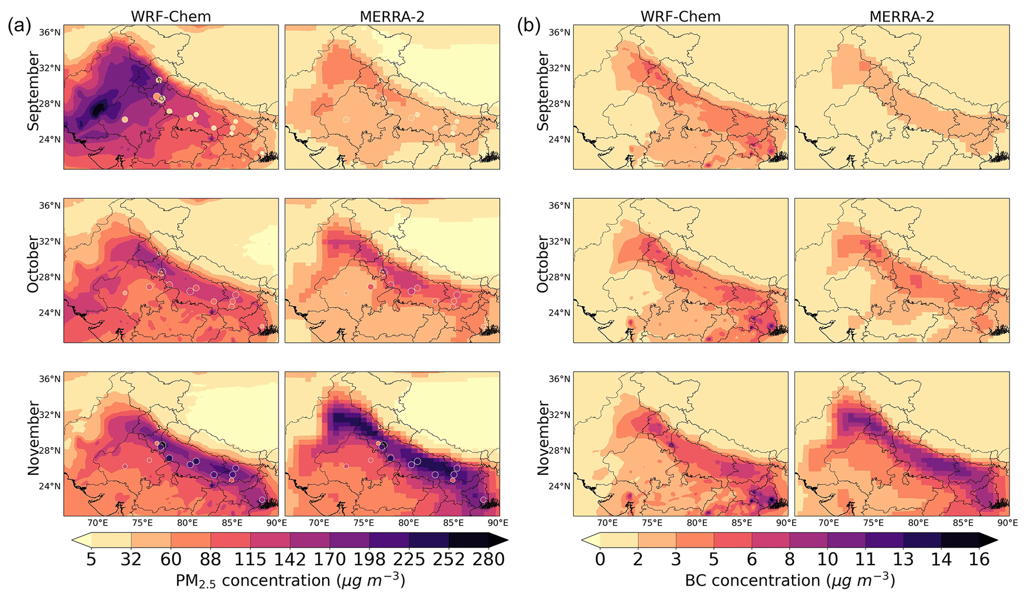
Figure 7 Spatial distributions of monthly mean concentrations (µg m⁻³) of (a) PM_2.5 and (b) black carbon from the WRF-Chem model and MERRA-2 for September to November 2016. The monthly mean PM_2.5 at the measurement sites is shown in circles in (a).

Table 6 Statistical summary of comparisons of concentrations (µg m⁻³) of PM_2.5 and black carbon from the WRF-Chem model and MERRA-2 from September to November 2016. The statistical metrics are mean bias (MB), normalized mean bias (NMB), mean absolute error (MAE), root mean square error (RMSE) and Pearson's correlation coefficient (r).

The high simulated PM_2.5 loading over some parts of north-western India during September is most likely due to erroneous dust uplift by overestimated winds from the Thar Desert in the west (Fig. S6), the major seasonal natural dust source region (Bali et al., 2021; M. Kumar et al., 2018). This overestimation could further be enhanced by the underestimation of dust deposition in the model arising from a dry bias over the land region in the domain (Ratnam and Kumar, 2005; Conibear et al., 2018). The notable change in modelled PM_2.5 over the dust source region along the western borders from September to November shows a strong seasonality in dust emissions in the model. Compared to WRF-Chem, MERRA-2 shows a slightly better comparison with monthly mean surface PM_2.5 (Fig. 7a) for individual monitoring sites, with smaller differences between the model-measured mean and WRF-Chem (especially for September).

In contrast, the highest BC concentrations occur along the IGP for all the months and increases from September to November (Fig. 7b). During October and November, the north-west and eastern parts of the IGP exhibit the highest PM_2.5 and BC concentrations in both datasets. Compared to MERRA-2, modelled BC shows more distinguishable spatial features including localized hotspots coinciding with densely populated major metropolitan and industrial cities with clusters of coal-fired power plants (Singh et al., 2018). For instance, conspicuous localized regions appear over dense urban centres like Ahmedabad, Delhi, Calcutta, the steel industrial city of Jamshedpur, Raipur with heavy mining, Singrauli with ore-processing industries in the upper central domain and Jharia coal belts in the east having clusters of coal-fired power plants. Overall, the spatial variabilities of BC and PM_2.5 are quite similar in both WRF-Chem and MERRA-2, with WRF-Chem estimating slightly lower PM_2.5 and BC in November over the majority of the IGP except over Delhi.

Table 7 Statistical summary of comparisons modelled and observed AOD at 550 nm derived from MODIS and at the four AERONET stations at an hourly temporal resolution between September and November 2016. The statistical metrics are mean bias (MB), normalized mean bias (NMB), mean absolute error (MAE), root mean square error (RMSE) and Pearson's correlation coefficient (r).

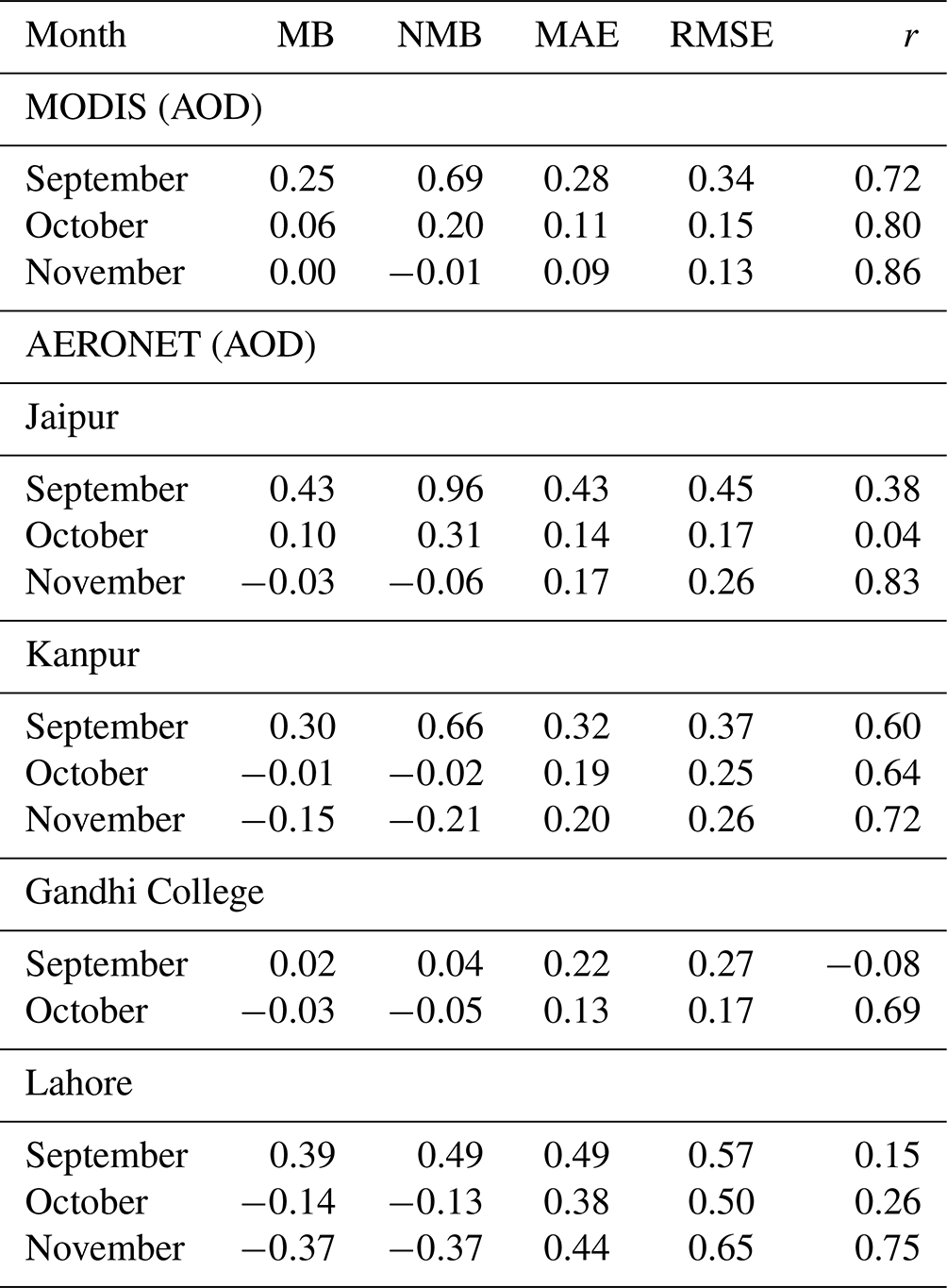
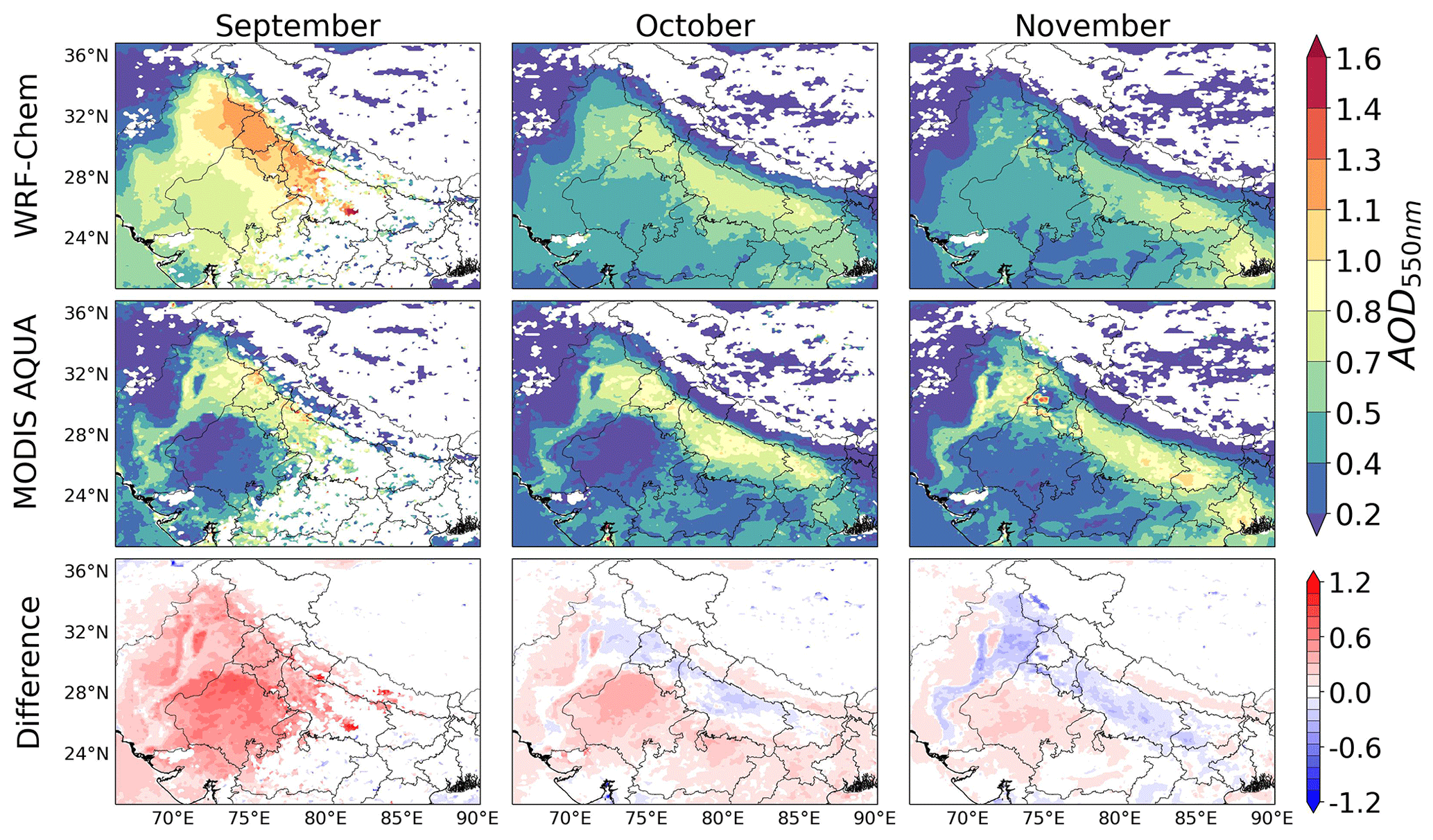
Figure 8 Spatial variation of monthly mean AOD at 550 nm derived from the model and MODIS sampled at local overpass times of 10.30 (Terra) and 13.30 (Aqua) for September to November 2016. Absolute differences of model minus satellite AOD are shown in the bottom row.

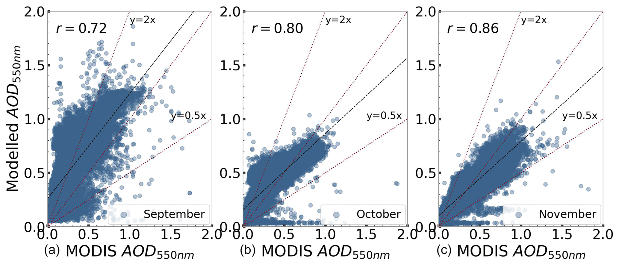
Figure 9 Scatter plots of monthly averaged model versus MODIS-derived AOD at 550 nm for the months (from left to right) September, October and November 2016. The 2:1, 1:1 and 1:2 lines (dashed red lines), the best-fit line (black line) and Pearson's correlation coefficient r are also shown for each month.

4.4 Evaluation of aerosol optical depth with satellite and AERONET observations

Figure 8 compares WRF-Chem-simulated and MODIS (Aqua)-retrieved monthly averaged distribution of AOD at 550 nm. The unitless quantity AOD is a measure of particle extinction within the atmospheric column from the surface to the top atmosphere and provides a useful spatial estimate of particle loading using satellite instruments. The spatial distributions of modelled and MODIS AOD agree well for all months (r≥0.72, Table 7), although regional biases similar to the MERRA-2 comparisons occur over northern and western parts of the domain. As with MERRA-2 PM_2.5 comparisons, during September the model captures the high AOD well (up to 1.2) over north-western India and along the borders with north-east Pakistan but predicts higher AOD over the western arid region (Fig. 8), indicated by the overall NMB of 0.69. The statistical evaluation metrics for all the months (Table 7) show there is a good overall agreement between modelled and satellite AOD, which gradually improves from September to November. In both model and satellite data, AOD values are generally low (<0.5) outside of the broader IGP region in all the months. Although the satellite AOD shows higher spatial variability, a good spatial correlation exists between the two datasets in October–November (r=0.80 and 0.86, respectively) (Fig. 9). The domain-averaged modelled AOD (0.39 and 0.34, respectively) during these months is comparable to satellite-retrieved AOD (0.32 and 0.34, respectively). Despite the overall underestimations during the biomass burning period of mid-October to mid-November, the model captures high AOD values over some small, localized parts in Punjab and Haryana in northern India and north-eastern Pakistan, though with slightly lower magnitudes. The higher AOD along the entire IGP region is more apparent from the satellite observations in November, which show AOD values reaching ∼2.0 (underestimated in the model by about 10 %) over parts of Punjab in the north and Uttar Pradesh and Bihar in the east (AOD > 1.8). Interestingly, the regional hotspots along the IGP region, over eastern Uttar Pradesh and eastern Bihar, as observed in modelled PM_2.5 maps during October–November, are evident in the MODIS AOD distribution but less discernible in modelled AOD maps (Fig. 8). It is important to note that the MODIS satellite overpass times of 10:30 and 13:30 LT limit comparisons to the afternoon each day. Therefore, it is the modelled meteorological conditions typical of daytime (deep PBL height, increased WS) that affect the modelled AOD column. In a similar model set-up over northern India, Roozitalab et al. (2021) and Kulkarni et al. (2020) found comparable estimates of modelled AOD distribution during the 2017 post-monsoon high-pollution event.

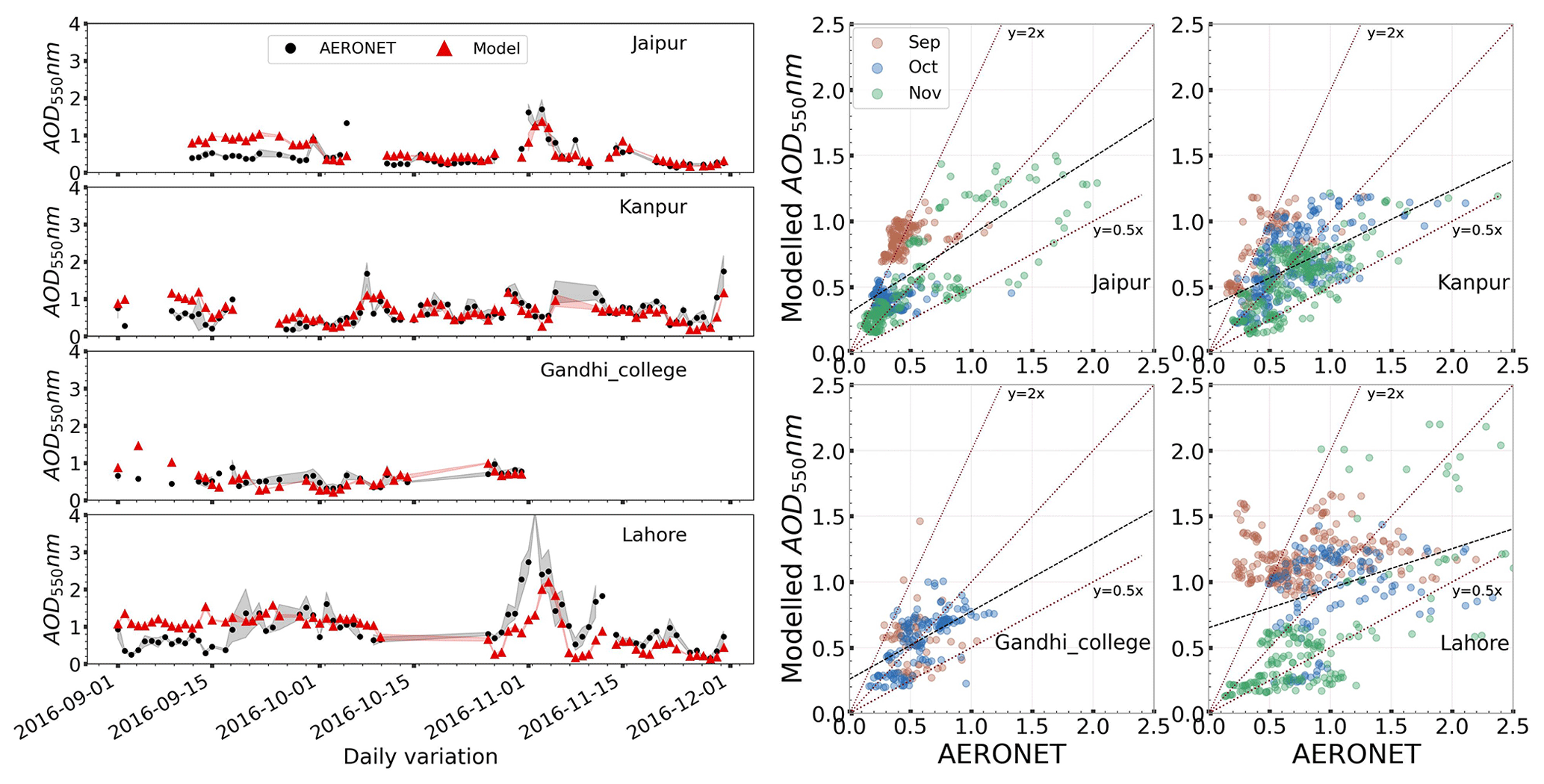
Figure 10 Time series (left panels) and scatter plots (right panels) of modelled and AERONET daily averaged AOD at 550 nm over the four AERONET stations shown in Fig. 1b for the period September to November 2016.

To further evaluate model skill in predicting the optical properties of aerosols, the modelled daily averaged AOD at 550 nm is compared in Fig. 10 against the four AERONET sites (Fig. 1b) in the study domain. There are missing data at all the sites, with Kanpur in the east and Jaipur in the west (both dense urban locations) having the most data coverage. The daily variabilities of AOD comparison with point observations show similar trends to those previously noted for comparison with satellite AOD and ground-based and MERRA-2 PM_2.5 comparisons. The model evaluation against AERONET AOD largely agrees with the PM_2.5 evaluations, including higher disparities seen for September, with a positive MB (0.02 to 0.43) across all the sites. However, the high daily averaged AERONET AOD (>1.0) at all sites during the high-pollution event at the start of November is captured reasonably well by the model except in Lahore, a large city in eastern Pakistan, where the model underestimates AOD the most. Of the four sites, crop residue burning occurs in Lahore (Kulkarni et al., 2020), which is also situated close to other biomass burning regions of north-western India. This AERONET site shows the highest observed (∼3.0) and modelled (∼2.0) AOD values during the high-pollution episode.

Additionally, to check for consistency between satellite and ground measurements, the time series of satellite, AERONET and modelled AOD at 550 nm at the four observation locations are shown in Fig. 11. To compare the three datasets, the data points corresponding to the local overpass time of MODIS are selected from the hourly AERONET and WRF-Chem datasets. The satellite AOD generally matches AERONET more closely at lower values and misses the magnitude of high AOD during high-pollution days. Earlier studies have attributed the inaccuracies in MODIS AOD retrievals to dense haze hanging over north India and the IGP region during severe pollution days (Mhawish et al., 2022). The modelled AOD captures the hourly AOD trend quite well but also underestimates AOD in absolute magnitude during high-pollution days across the sites. Overall, the modelled AOD agrees well with satellite and ground observations during October and November despite some underestimations in absolute magnitudes.

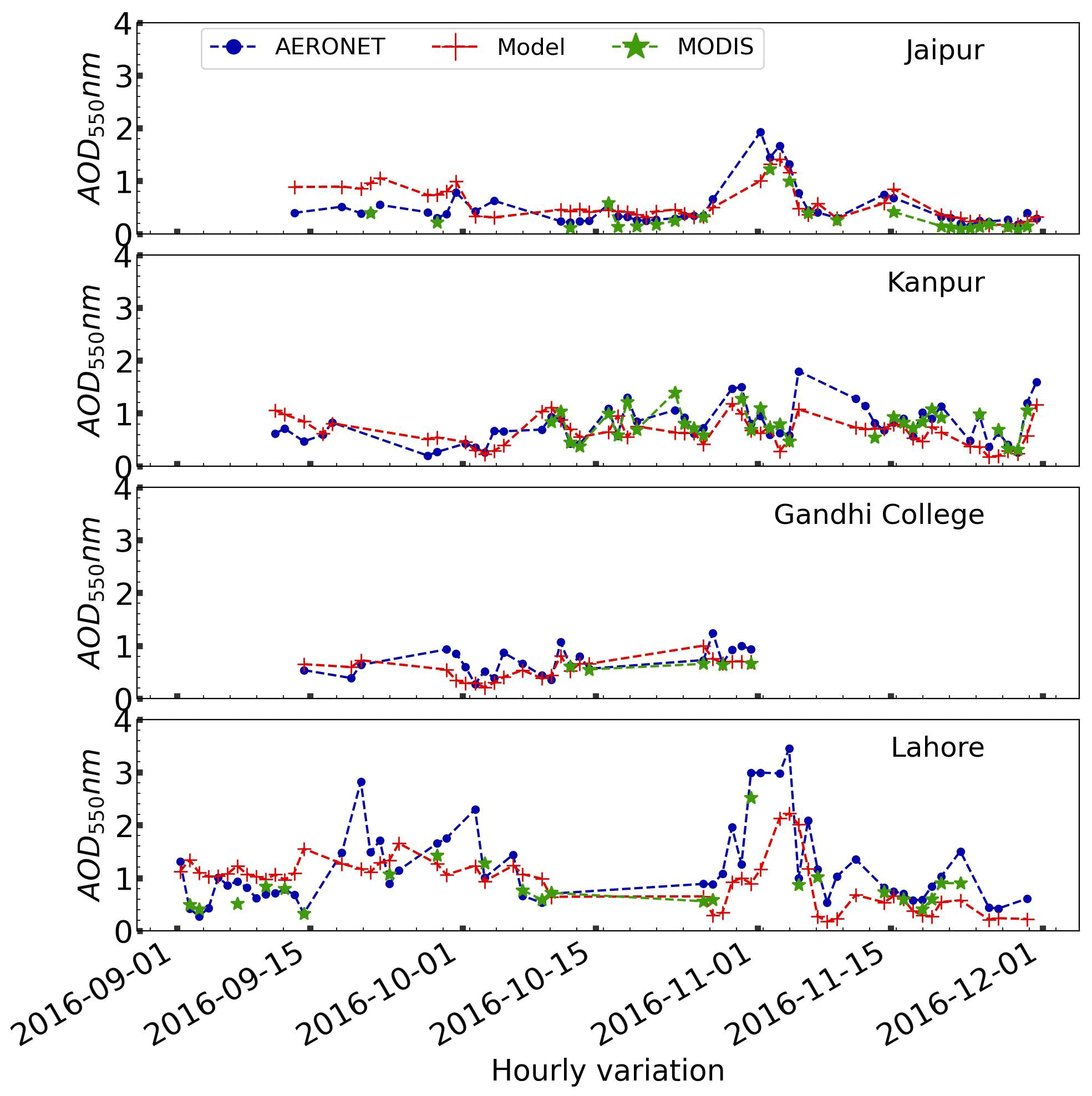
Figure 11 Time series of MODIS-retrieved (green), modelled (red) and AERONET (blue) AOD at 550 nm sampled at 13:30 IST over the four AERONET stations shown in Fig. 1b: from top to bottom, Jaipur, Kanpur, Gandhi College and Lahore.

4.5 Discussion

The discrepancies in model–observation particulate matter comparisons for September have also been noted in other studies for India and suggest inaccuracies in modelling moisture transport during the monsoon season, which affects particle deposition and washout (Conibear et al., 2018; Mogno et al., 2021). Furthermore, in 2016, almost all the ground stations were in urban locations of the IGP region, which prevents the evaluation of the model at more spatially representative rural locations. In addition, nearly all the measurement sites are in or near dense urban areas, with heavy influences from traffic and local anthropogenic activities (for example, trash burning and residential cooking), which may not be fully reflected in the monthly anthropogenic emission inputs. The sudden jumps in particulate matter during an extreme-pollution event are especially difficult to capture within the model (despite adequate meteorological fields) without updated emissions estimates and knowledge of dynamic local activity data (for instance, diurnal activity profiles specific to Indian regions). For example, residential emissions are a major contributor to poor air quality in rural and suburban areas in northern India, with an estimated 16 % to 80 % contribution towards SOA components of PM_2.5 (Rooney et al., 2019).

Diurnally, the nocturnal biases in wind speeds in the model allow for an increased dispersal of the pollutants near the surface, leading to underestimated PM_2.5 concentrations during the night. Furthermore, the inaccuracies in simulating individual fractions of total PM_2.5 also add to the observed model biases; for example, high contributions from dust in the MOSAIC scheme could lead to overestimations (Georgiou et al., 2018). Overestimated modelled dust aerosols were also observed by Kalenderski et al. (2013) and Zhao et al. (2010), who tuned the online dust emission flux calculation based on region-specific AERONET measurements for a dust event and found modelled AOD estimates to improve. The lack of aqueous-phase chemistry in our model framework further adds some biases in reproducing accurate amounts of secondary aerosol components of PM (such as SO${}_{\mathrm{4}}^{\mathrm{2}-}$, NH${}_{\mathrm{4}}^{+}$ and NO${}_{\mathrm{3}}^{-}$) and their subsequent scavenging by aqueous chemistry in the cloud or water droplets (Tuccella et al., 2012; Balzarini et al., 2015). Furthermore, underestimations in modelled PM_2.5 concentrations across Delhi could also be due to the lack of input emissions of hydrogen chloride (HCl) gas, typically from seasonal local rubbish and crop residue burning, which adds substantial chloride aerosols to total PM_2.5 by its partitioning between gas and aerosol phases (Cash et al., 2021; Lalchandani et al., 2022; Pawar et al., 2023). The temporal mismatch due to changes in emissions between the anthropogenic emissions inventory (2010) and the simulated year (2016) also contributes to the likely underestimation in the modelled PM_2.5 and its components for our study period. Notably, a few studies simulating other years also report positive seasonal biases in simulating surface and column concentrations of trace gases like NO_x (Kumar et al., 2012a) and concentrations of SO₂ (Conibear et al., 2018) over urban areas in India . These biases further contribute to uncertainties in simulating reactive trace gas and secondary PM_2.5 subspecies.

Significant post-harvest crop residue burning takes place in north-western states of India from late October to mid-November (Jethva et al., 2019), which impacts the air quality locally as well as in downwind regions of central and eastern IGP (Bhardwaj et al., 2016; Kanawade et al., 2020; Kulkarni et al., 2020; Singh et al., 2021; Mhawish et al., 2022; Govardhan et al., 2023a). Other uncertainties in simulating PM_2.5 concentrations arise from errors in scaling biomass burning emissions estimates, which largely depend on the limited number of daily satellite-based retrievals and are sometimes compromised by dense smoke from fires being misrepresented as cloud cover in the detection algorithm (Cusworth et al., 2018). In their study, Singh et al. (2021) report the annual mean contribution of biomass burning to PM_2.5 over India to be 8 % but with a strong seasonal dependence (up to 39 % in October–November in Delhi). As previously discussed in the literature, MODIS fire detection is susceptible to missing small fires like agricultural burning (Cusworth et al., 2018; Roozitalab et al., 2021). In addition to the surface measurements, comparisons with MERRA-2 products highlight a good agreement between the WRF-Chem simulations and the reanalysis approach of employing satellite data assimilations. Navinya et al. (2020) and others, however, find MERRA-2 to underestimate simulated PM_2.5 over India in comparison to the measurements. As noted in Sect. 2.5, several factors need to be considered when comparing the WRF-Chem aerosol concentrations with MERRA-2 reanalysis products. These include (but are not limited to) a coarser resolution of MERRA-2; limited observations data available for assimilation; input anthropogenic emissions lacking seasonal variability; the GOCART chemistry scheme missing nitrate and SOA treatment; and the quality of aerosol transport dynamics from the GEOS-5/GOCART model, wherein the reanalysed aerosol mass concentrations are not directly constrained by the observations as is the case with the AOD (Buchard et al., 2017). These points, therefore, suggest the use of aerosol assimilation capabilities in combination with the chemistry representing complex aerosol processes is potentially a more accurate way to predict air quality across polluted regions such as northern India.

Overall, the evaluation of the WRF-Chem-simulated chemistry demonstrates adequate performance during October and November for PM_2.5 and is found to be suitable for investigating the atmospheric dynamics during extreme-pollution events. The modelled results presented here, and in other studies of pollution episodes and aerosol climatology over India, clearly show that the October–November period has higher aerosol loading over most of the domain compared to other times of the year. A mix of factors like emission patterns, meteorology shifts and topography intensify the existing high-pollution levels in some parts of India (Kulkarni et al., 2020; M. Kumar et al., 2018; Mhawish et al., 2022; Kanawade et al., 2020). Sawlani et al. (2019) and Kanawade et al. (2020) attribute the 2016 haze episode to a mix of coinciding factors: local emissions from fireworks, enhanced fire counts from agricultural crop residue burning in north-western states, stagnant conditions resulting from low temperatures, shallow PBL, weaker north-westerly winds and high ambient RH. The crop residue burning in 2016 (over Punjab, Haryana and Uttar Pradesh in north-west India and Pakistan) detected by combined VIIRS and MODIS sensors reveals higher total burning events by up to 30 % and 41 % compared to 2017 and 2018, respectively (Chhabra et al., 2019). Similar high-pollution events have been reported during post-monsoon months in later years (Dekker et al., 2019; Kulkarni et al., 2020; Takigawa et al., 2020; Roozitalab et al., 2021; Beig et al., 2021; Mhawish et al., 2022). Additionally, a few studies also report a layer of biomass burning smoke aerosols at 2–3 km altitude above the IGP region using CALIPSO (Cloud-Aerosol Lidar and Infrared Pathfinder Satellite Observations) retrievals (Shaik et al., 2019; M. Kumar et al., 2018).

5 Conclusions

We comprehensively compare the WRF-Chem v4.2.1 modelled meteorology and aerosol chemistry with a wide range of observational data that include ground-based, satellite and reanalysis products over northern India. The simulations are performed at a spatial resolution of 12 km for the 2016 monsoon (September) to post-monsoon (October–November) transition, with a focus on the severe haze pollution episode from 30 October to 7 November.

The meteorological fields show strong seasonal and spatial variability over the IGP region, with a marked decrease in temperature, WS and PBLH from monsoon to post-monsoon, most notably for PBLH. Overall, we find that the model accurately represents meteorology during the afternoon hours. The surface daily and diurnal trend in temperature is best reproduced by the model, followed by relative humidity, with negligible biases across all sites. In contrast, daily mean model wind speed is widely biased high (by 0.5–0.8 m s⁻¹), largely due to strong night-time overestimations (up to 1.5 m s⁻¹), while the afternoon WS is reasonably reproduced by the model. This suggests a potential model failure in surface layer decoupling at night.

Comparison of upper-air meteorology with radiosonde profiles shows negligible biases and excellent correlations for temperature and virtual potential temperature (r>0.9) across all sites. The model overestimates wind speed in the lowest layers, consistent with surface observation comparisons whilst matching well with observed WS aloft. In comparison to MERRA-2 reanalysis products, modelled PBLH generally has negative mean bias of >25 % in all the months but agrees well spatially.

Modelled and observed PM_2.5 concentrations show good agreement (except during September) with overall slightly better correlations for 8 sites averaged across Delhi (r>0.6) compared to 12 sites across the remaining domain (r>0.5). In September, model concentrations show large biases due to overestimation in dust generation over the western arid region and possible long-range transport across the measurement sites.

The model simulates the high-pollution episode with notable peaks in daily mean PM_2.5 concentrations but underestimates the exceptionally high observed daily PM_2.5 (300–750 µg m⁻³) by a factor of 2–3. Despite the accurate representation of the vertical temperature gradient, the model underestimates high surface PM_2.5 concentrations due to stronger simulated WS favouring the dispersion of the surface pollutants, together with uncertainties in the emissions inventories. Both the model and surface measurements show that Delhi experiences the highest PM_2.5 concentrations during the severe pollution episode, followed by the regional dispersal of pollutants downwind. During the episode, daily simulated anthropogenic PM_2.5 composition comprised high fractions of nitrate (5 %–25 %) and secondary organic aerosols (10 %–20 %), consistent with previous measurement and modelling studies. The contribution of BC and primary organic matter to the total simulated PM_2.5 mass also increases in November.

Comparison with MERRA-2 reanalysis data shows the spatiotemporal distribution of surface PM_2.5 to have systematic high biases in September along the dry western region of the domain and low bias in October–November in the IGP region. However, the model captures the high PM_2.5 and BC concentrations quite well over the IGP, including Delhi and upwind biomass burning regions during November. Variability in modelled AOD compared with satellite retrievals from MODIS is captured very well with r≥0.8 in October–November. The model likewise compares well with ground-based AERONET measurements of daily AOD (r≥0.7) across all sites except during September.

Our evaluations consistently reveal the best performance of the model in simulating PM_2.5 and BC concentrations is for November followed by October, with model underestimations largely stemming from the extreme episodic nature of the pollution event. The lack of measurement data for individual PM_2.5 components and the limited spatial coverage of measurement sites restrict the extent of the evaluation of this period. Overall, however, the model is found adequate for investigation of the vertical distribution of particle components and their interactions with meteorology through sensitivity simulations, including investigation of different emissions datasets, which forms part of our future work. Our results also suggest that improved diurnal characterization of boundary layer processes could considerably enhance the model performance over this region.