the Creative Commons Attribution 4.0 License.
the Creative Commons Attribution 4.0 License.
 | 20 Feb 2024
Investigation of the renewed methane growth post-2007 with high-resolution 3-D variational inverse modeling and isotopic constraints
Marielle Saunois
Antoine Berchet
Isabelle Pison
Philippe Bousquet
We investigate the causes of the renewed growth of atmospheric methane (CH4) amount fractions after 2007 by using variational inverse modeling with a three-dimensional chemistry-transport model. Together with CH4 amount fraction data, we use the additional information provided by observations of CH4 isotopic compositions (13C : 12C and D : H) to better differentiate between the emission categories compared to the differentiation achieved by assimilating CH4 amount fractions alone. Our system allows us to optimize either the CH4 emissions only or both the emissions and the source isotopic signatures (δsource(13C,CH4) and δsource(D,CH4)) of five emission categories. Consequently, we also assess, for the first time, the influence of applying random errors to both emissions and source signatures in an inversion framework. As the computational cost of a single inversion is high at present, the methodology applied to prescribe source signature uncertainties is simple, so it can serve as a basis for future work. Here, we investigate the post-2007 increase in atmospheric CH4 using the differences between 2002–2007 and 2007–2014. When random uncertainties in source isotopic signatures are accounted for, our results suggest that the post-2007 increase (here defined using the two periods 2002–2007 and 2007–2014) in atmospheric CH4 was caused by increases in emissions from (1) fossil sources (51 % of the net increase in emissions) and (2) agriculture and waste sources (49 %), which were slightly compensated for by a small decrease in biofuel- and biomass-burning emissions. The conclusions are very similar when assimilating CH4 amount fractions alone, suggesting either that random uncertainties in source signatures are too large at present to impose any additional constraint on the inversion problem or that we overestimate these uncertainties in our setups. On the other hand, if the source isotopic signatures are considered to be perfectly known (i.e., ignoring their uncertainties), the relative contributions of the different emission categories are significantly changed. Compared to the inversion where random uncertainties are accounted for, fossil emissions and biofuel- and biomass-burning emissions are increased by 24 % and 41 %, respectively, on average over 2002–2014. Wetland emissions and agricultural and waste emissions are decreased by 14 % and 7 %, respectively. Also, in this case, our results suggest that the increase in CH4 amount fractions after 2007 (despite a large decrease in biofuel- and biomass-burning emissions) was caused by increases in emissions from (1) fossil fuels (46 %), (2) agriculture and waste (37 %), and (3) wetlands (17 %). Additionally, some other sensitivity tests have been performed. While the prescribed interannual variability in OH can have a large impact on the results, assimilating δ(D,CH4) observations in addition to the other constraints has only a minor influence. Using all the information derived from these tests, the net increase in emissions is still primarily attributed to fossil sources (50 ± 3 %) and agriculture and waste sources (47 ± 5 %). Although our methods have room for improvement, these results illustrate the full capacity of our inversion framework, which can be used to consistently account for random uncertainties in both emissions and source signatures.
- Article
(7371 KB) - Full-text XML
- BibTeX
- EndNote


Atmospheric methane (CH4) has a large influence on both climate and atmospheric chemistry. The globally averaged tropospheric CH4 amount fraction has increased by a factor of 2.6 since pre-industrial times (Gulev et al., 2021), and it reached a new high of 1912 nmol mol−1 in 2022 (global average from marine surface sites; Lan et al., 2023). Neglecting indirect effects related to ozone, water vapor and nitrogen oxide production, a consequence of this large increase in CH4 amount fractions since the pre-industrial era is that CH4 now contributes 16 % of the current radiative forcing from well-mixed greenhouse gases (carbon dioxide, methane, nitrous oxide, halogens) (Forster et al., 2021). CH4 therefore makes the second largest contribution to the additional greenhouse effect, behind carbon dioxide (CO2). CH4 amount fractions increased quasi-continuously since the pre-industrial era until 1999, but then stabilized between 1999 and 2006. The growth resumed after 2007, at a rate exceeding 10 for some years. Nisbet et al. (2019) pointed out that the dramatic increase in the CH4 burden is contrary to pathways compatible with the goals of the Paris Agreement of the 2015 United Nations Framework Convention on Climate Change and that urgent action is required to bring CH4 back to a pathway more in line with the goals of the Paris Agreement. A proper understanding of the CH4 budget could highly facilitate such actions by increasing the effectiveness of mitigation policies.
CH4 is emitted into the atmosphere by multiple sources (wetlands, livestock, rice cultivation, waste, fossil fuel exploitation, biomass burning, …), with distinct processes involved (microbial, thermogenic, pyrogenic). This species is mainly removed from the atmosphere through oxidation by the hydroxyl radical (OH), which represents about 92 % of the total sink (Saunois et al., 2020; Thanwerdas et al., 2022b). Other sinks include oxidation by atomic oxygen (O1D), chlorine (Cl) and methanotrophs in the soil, which contribute about 1.5 %, 1.5 % and 5 %, respectively, to the total removal of CH4 (Saunois et al., 2020; Thanwerdas et al., 2022b). Note that these numbers come with non-negligible uncertainties and vary from one study to another.
Estimating these sources and sinks is challenging, especially at the global scale, yet it is necessary to better understand the CH4 budget and to anticipate its evolution. The scientific community has developed two approaches to estimate CH4 emissions at different scales. On the one hand, bottom-up approaches aim to estimate these emissions using both inventories that combine statistical activity data with emission factors for anthropogenic emissions (e.g., Höglund-Isaksson, 2012, 2017; Janssens-Maenhout et al., 2019) and process-based models for natural and fire emissions (e.g., van der Werf et al., 2017; Poulter et al., 2017). Bottom-up estimates provide valuable sectorial and regional information, although their global emissions are not constrained by atmospheric observations. On the other hand, top-down approaches use inversion methods (Newsam and Enting, 1988; Enting and Newsam, 1990) and chemistry-transport models (CTMs) to statistically optimize model parameters (e.g., emissions) and minimize model–observation differences (e.g., Houweling et al., 2017, and references therein). These approaches provide posterior estimates that are consistent with both atmospheric observations (e.g., CH4 amount fractions) and prior estimates (typically derived from bottom-up estimates). The inversion problem is considered to be “ill posed” because a wide range of surface flux configurations can equally well explain the observational data in the atmosphere. Since the 1980s, surface monitoring networks have nevertheless significantly increased the spatial coverage and the precision of their observations, narrowing the range of possible flux configurations and improving the relevance of inversion methods.
Although Saunois et al. (2020) recently showed that the consistency between top-down and bottom-up estimates has improved over time, the 1999–2006 plateau and the subsequent renewed growth still generate considerable attention and controversy (Rice et al., 2016; Schwietzke et al., 2016; Schaefer et al., 2016; Nisbet et al., 2016; Patra et al., 2016; Bader et al., 2017; Turner et al., 2017; Rigby et al., 2017; Worden et al., 2017; Saunois et al., 2017; Morimoto et al., 2017; McNorton et al., 2018; Thompson et al., 2018; Schaefer, 2019; Nisbet et al., 2019; Fujita et al., 2020; Zimmermann et al., 2020; Jackson et al., 2020; Chandra et al., 2021). Most of these studies suggest that the renewed growth is partially explained by an increase in microbial emissions (wetlands, livestock and/or rice cultivation), while some of them localized the increase to the tropics (Nisbet et al., 2016; Patra et al., 2016; Schaefer et al., 2016; Schwietzke et al., 2016). Multiple studies have also concluded that the renewed growth was driven by an increase in both microbial and fossil fuel emissions (Rice et al., 2016; Patra et al., 2016; Bader et al., 2017; Worden et al., 2017; Saunois et al., 2017; McNorton et al., 2018; Thompson et al., 2018; Jackson et al., 2020; Chandra et al., 2021; Lan et al., 2021; Basu et al., 2022), although they provide a very wide range of individual contributions. An increase in fossil fuel emissions was also supported by an independent work that used ethane-based approaches (Hausmann et al., 2016). However, other studies found that these emissions decreased or stabilized (Schwietzke et al., 2016; Schaefer et al., 2016; Fujita et al., 2020) over the period of renewed growth. Some studies also found that an increase in emissions was not the main driver and that a large decrease in OH concentrations could explain the recent variations (Turner et al., 2017; Rigby et al., 2017).
Such controversy partly arises from the difficulty in separating contributions from individual CH4 sources. Despite the high number of observations over some regions, many of the sources are co-located, and isolating the contribution from each source to the local increase in CH4 amount fractions is challenging. Atmospheric carbon and hydrogen isotope compositions, δ(13C,CH4) and δ(D,CH4), can help us to differentiate co-emitted emission categories because each CH4 production process (microbial, thermogenic, pyrogenic) has its own characteristic isotopic signature (Sherwood et al., 2021, 2017). δ(13C,CH4) and δ(D,CH4) are generally defined as the deviation of the sample's atomic isotopic ratio ( or relative to a specific standard ratio:
Here, X(12CH4), X(13CH4), X(CH3D) and X(CH4) denote the 12CH4, 13CH4, CH3D and CH4 amount fractions, respectively. is the standard ratio of Pee Dee Belemnite (PDB) (Craig, 1957) and is the Vienna Standard Mean Ocean Water (VSMOW) ratio (Hagemann et al., 1970; Wit et al., 1980). δ(13C,CH4) and δ(D,CH4) are expressed in ‰. Broadly summarized, CH4 sources have a δ(13C,CH4) isotopic signature, hereinafter denoted by δsource(13C,CH4), of between −65 ‰ and −55 ‰ for microbial sources, between −45 ‰ and −35 ‰ for thermogenic sources, and between −25 ‰ and −15 ‰ for pyrogenic sources (Sherwood et al., 2021, 2017). However, the full distributions of isotopic signatures are wider than these ranges, with overlaps between the distributions for the different production processes. Similarly, there are different δsource(D,CH4) distributions for different production processes. Their approximate ranges are between −350 ‰ and −100 ‰ for thermogenic sources, between −400 ‰ and −250 ‰ for microbial sources, and between −250 ‰ and −175 ‰ for pyrogenic sources (Sherwood et al., 2021, 2017). Notably, the microbial and thermogenic δsource(D,CH4) distributions show a smaller overlap than that of the corresponding distributions for δsource(13C,CH4), and thermogenic sources have signatures that are less distinguishable from others.
Variations in atmospheric isotopic composition are not caused by sources only. Reactions between sink species (OH, O1D and Cl) and CH4 have rates that depend on the isotopologue. This effect is called fractionation and is represented, for a specific reaction, using the ratio of the reaction rates achieved with the lightest and the heaviest members of a couple of isotopologues (e.g., 12CH4 and 13CH4). The fractionation effect explains why the atmospheric isotopic composition is not equal to the flux-weighted mean source signature for all the CH4 sources. It acts to shift this mean source composition towards less negative values when CH4 enters the atmosphere and gets removed by the sinks. This effect is particularly important for δsource(D,CH4) because the flux-weighted mean source signature and the observed isotopic composition are approximately −330 ‰ and −95 ‰, respectively (Sherwood et al., 2017). For δ(13C,CH4), this effect is smaller, shifting the source signature from approximately −53.6 ‰ to −47.3 ‰ in the atmosphere (Sherwood et al., 2017).
The post-2007 CH4 increase is notably associated with a decrease of 0.2 ‰–0.3 ‰ in δ(13C,CH4) since 2007 (Rice et al., 2016; Schaefer et al., 2016; Nisbet et al., 2016, 2019). Such significant isotopic variations provide an additional atmospheric constraint to better estimate the relative contribution of CH4 sources to this renewed atmospheric CH4 growth. Some of the aforementioned studies that focused on the drivers of both the plateau and the renewed growth were conducted using inversion methods that included isotopic constraints. Those studies implemented either three-dimensional (3-D) CTMs coupled with analytical inversion methods that estimated emissions for aggregated large regions only (Rice et al., 2016; McNorton et al., 2018), box models with analytical inversion methods (Schwietzke et al., 2016; Turner et al., 2017; Rigby et al., 2017), or 2-D CTMs with variational inversion methods (Thompson et al., 2018). Analytical methods are not fit to use for large-dimension problems, i.e., those with both a large number of optimized variables and observations, and these methods generally need to aggregate emissions across large regions. By contrast, variational inversion methods can easily both optimize the emissions at the grid-cell scale (the model's horizontal resolution) and assimilate large observational datasets. Furthermore, 3-D CTMs can better capture the spatial variability of sources, sinks and observations than box models and 2-D CTMs.
This paper utilizes the system designed by Thanwerdas et al. (2022a) to investigate changes in CH4 emissions from 1998–2018 by running 3-D variational inversions at the grid-cell scale. The original system has been improved and can assimilate both 13CH4 : 12CH4 and CH3D : CH4 observations. The optimization of source isotopic signatures is also tested here because, at present, they remain a large source of uncertainty (Sherwood et al., 2017; Turner et al., 2017; Feinberg et al., 2018) that should be considered.
In Sect. 2, we provide a detailed methodology describing the inversions performed in this study. In Sect. 3, the results are presented. First, we evaluate the agreement between model outputs and assimilated data and compare our simulations to independent data. As a second step, we provide an analysis of posterior emissions and isotopic signatures estimated by the reference inversion and the sensitivity tests. To the best of our knowledge, the methodology developed by Basu et al. (2022) is the only one that presents high similarities to ours. They investigated the same problem with a variational inversion framework and a 3-D CTM. However, substantial differences exist between our techniques. In their paper, they included a comparison between their work and Thanwerdas et al. (2022a). Based on our new results, we propose an updated comparison in Sect. 3.9. Conclusions are drawn and a discussion is provided in Sect. 4.
2.1 The chemistry-transport model
The general circulation model (GCM) LMDz is the atmospheric component of the coupled model from the Institut Pierre-Simon Laplace (IPSL-CM), developed at the Laboratoire de Météorologie Dynamique (LMD) (Hourdin et al., 2006). The version of LMDz used here is an offline version dedicated to the inversion framework created by Chevallier et al. (2005): the precalculated meteorological fields provided by the online version of LMDz are given as input to the model, considerably reducing the computation time. The model is built at a horizontal resolution of 3.8∘ × 1.9∘ (96 grid cells in longitude and latitude), with 39 hybrid sigma-pressure levels reaching an altitude of about 75 km. The time step of the model is 30 min and the output values have a resolution of 3 h. Horizontal winds are nudged towards the ECMWF meteorological analyses (ERA-Interim) in the online version of the model. Vertical diffusion is parameterized by the local approach of Louis (1979), and deep convection processes are parameterized by the scheme of Tiedtke (1989). The offline model LMDz is coupled with the Simplified Atmospheric Chemistry System (SACS) to represent CH4 oxidation by radicals (Pison et al., 2009; Thanwerdas et al., 2022a).
We simulate atmospheric 12CH4 and 13CH4 amount fractions to retrieve both the CH4 amount fractions and the δ(13C,CH4) signal. Four clumped isotopologues (12CH4, 12CH3D, 13CH4 and 13CH3D) are simulated in one sensitivity simulation (see Sect. 2.7) to retrieve both the δ(13C,CH4) and δ(D,CH4) compositions.
Oxidations by OH, O(1D) and Cl are included in the chemical scheme of LMDz-SACS. Time-varying 3-D fields of OH and O(1D) with daily resolution, simulated beforehand with the LMDz-INCA chemistry model (Hauglustaine et al., 2004), are prescribed for each oxidant species to simulate the associated chemical loss. The same meteorological data were used for generating these fields and running the simulations presented in this study.
The resulting OH field, named OH-INCA, exhibits a global mean tropospheric mass-weighted concentration of 11.1 × 105 cm−3 over 1998–2018, consistent with the previous estimates from Zhao et al. (2019) (11.7 × 105 cm−3) and Prather et al. (2012) ((11.2 ± 1.3) × 105 cm−3) and well within the range derived from the Atmospheric Chemistry and Climate Model Intercomparison Project (ACCMIP) (10.3–13.4 × 105 cm−3; Voulgarakis et al., 2013). It is, however, slightly larger than the very recent estimate from Zhao et al. (2023), obtained by constraining OH with observations of its precursors. The interhemispheric ratio is 1.14, lower than the mean value of 1.3 inferred by Zhao et al. (2019) but more consistent with recent estimates from Zhao et al. (2023) and an interhemispheric parity obtained from methyl-chloroform-based inversions (Bousquet et al., 2005; Patra et al., 2014). Global concentrations of OH-INCA increased by 4 % between 2002 and 2014.
As suggested by Thanwerdas et al. (2022b), the Cl concentrations derived by Wang et al. (2021) are prescribed here for all simulations. Their work suggests that the Cl sink accounts for only 0.8 % of the total CH4 oxidation, which is lower than other estimates used in the literature (1.8 %–5 %; Allan et al., 2007; Sherwen et al., 2016; Hossaini et al., 2016).
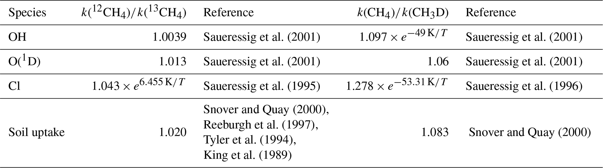
The fractionation effect must also be represented in the modeling framework. Table 1 provides the fractionation coefficients applied for each loss reaction. For the OH sink, we adopted the estimate derived by Saueressig et al. (2001). Burkholder (2019) recommends using the Saueressig et al. (2001) rates but suggests increasing the uncertainty in the OH fractionation to account for the estimate (1.0054) from Cantrell et al. (1990). As shown by Basu et al. (2022), switching estimates from that of Saueressig et al. (2001) to that of Cantrell et al. (1990) has a large influence on the results, despite the fact that those authors did not optimize source signatures in their setup. As Saueressig et al. (2001) indicate that their data is of considerably higher experimental precision and reproducibility than that from previous studies, in particular Cantrell et al. (1990), we prefer to allocate computational time to a sensitivity inversion testing a different OH field rather than testing a different OH fractionation coefficient. In addition, these estimates of fractionation coefficients come with uncertainty ranges that we could also consider in our inversions (e.g., with a Monte Carlo approach). In our case, the main limitation remains the large computational cost of one inversion (see Sect. 2.9). In the future, we hope to be able to increase the number of sensitivity tests and account for this uncertainty. For this work, the values we adopt are the best estimates for each fractionation coefficient.
Saueressig et al. (2001)Saueressig et al. (2001)Saueressig et al. (2001)Saueressig et al. (2001)Saueressig et al. (1995)Saueressig et al. (1996)Snover and Quay (2000)Snover and Quay (2000)Reeburgh et al. (1997)Tyler et al. (1994)King et al. (1989)Table 1Fractionation coefficients for loss reactions with OH, O(1D) and Cl and soil uptake. T denotes the temperature.
2.2 Inverse modeling with a variational approach
Inversions were performed using the Community Inversion Framework (CIF; Berchet et al., 2021). This framework was designed to rationalize and bridge development efforts made by the scientific community within the same flexible, transparent and open-source system. This system was recently enhanced by Thanwerdas et al. (2022a) to allow it to assimilate δ(13C,CH4) together with CH4 observations and to optimize both CH4 emissions and the source signatures δsource(13C,CH4) at the same time. For the purpose of this study, δ(13C,CH4) and δ(D,CH4) observations are assimilated together in the same inversion, and the system optimizes both the source signatures (δsource(13C,CH4) and δsource(D,CH4)).
The notations introduced here to describe the variational inversion method follow the convention defined by Ide et al. (1997) and Rayner et al. (2019). x is the control vector and includes all the variables optimized by the inversion system. Prior information about the control variables is included in the vector xb. Its associated errors are assumed to be unbiased and Gaussian and are described within the error covariance matrix B.
Here, the observation vector yo includes all available observations, namely the atmospheric CH4 amount fraction, δ(13C,CH4) and δ(D,CH4) data for one sensitivity test. The associated errors are also assumed to be unbiased and Gaussian and are described within the error covariance matrix R. This matrix accounts for all errors contributing to mismatches between simulated and observed values.
ℋ is the observation operator that projects the control vector x into the observation space. This operator mainly consists of the CTM but is also followed by spatial, time and isotope-conversion operators. Following Thanwerdas et al. (2022a), prescribed source signatures and CH4 fluxes are first combined to generate isotope fluxes. These fluxes are then fed to the model to simulate the mixing ratios of the different isotopes over the time period considered. After the forward run, the simulated fields are interpolated to produce simulated equivalents of the observed amount fractions and isotopic compositions at specific locations and times, ensuring that a comparison between simulations and observations is possible. Adjoint versions of these forward operations are also implemented in order to perform the complementary adjoint run.
In a variational formulation of the inversion problem that allows ℋ to be nonlinear, the cost function J is defined as
Here, the minimum of J is reached iteratively with the descent algorithm M1QN3 (Gilbert and Lemaréchal, 1989), which requires several computations (40–50) of the gradient of J with respect to the control vector x:
ℋ* denotes the adjoint operator of ℋ.
The reference inversion (INV_REF) assimilates CH4 and δ(13C,CH4) observations over 1998–2018. CH4 emissions and δ(13C,CH4) source signatures for five categories of emissions – biofuel and biomass burning (BB), wetlands (WET), fossil fuels and geological sources (FFG), agriculture and waste (AGW), and other natural sources (NAT) – are optimized. The initial conditions for CH4 and δ(13C,CH4) are also optimized (see Sect. 2.6).
2.3 Prior emissions and uncertainties
For prior CH4 emissions, we adopt the bottom-up estimates compiled for the inversions performed as part of the Global Methane Budget and described in detail in Saunois et al. (2020). In short, anthropogenic (including biofuel) and fire emissions are based on EDGARv4.3.2 (Emissions Database for Global Atmospheric Research version 4.3.2; Janssens-Maenhout et al., 2019) and GFED4s (Global Fire Emissions Database version 4s; van der Werf et al., 2017), respectively. Statistics from British Petroleum (BP) and the Food and Agriculture Organization of the United Nations (FAO) have been used to extend EDGARv4.3.2 (which ends in 2012) until 2017. The natural source emissions are based on averaged literature values: Poulter et al. (2017) for wetlands, Kirschke et al. (2013) for termites, and Lambert and Schmidt (1993) and Etiope (2015) for geological (onshore) sources and oceanic sources that include geological (offshore) and hydrate sources. Prior emissions for 2018 are set equal to the emissions in 2017. Globally averaged emissions over 1998–2018 are listed in Table 2.
BB emissions are the combination of biomass-burning emissions from GFED4s and biofuel-burning emissions from EDGARv4.3.2. FFG emissions are the combination of oil, gas, coal, industrial and transport emissions from EDGARv4.3.2 and geological (onshore) source emissions from Etiope (2015), whose global emissions were scaled down to 15.0 Tg a−1 in the protocol of Saunois et al. (2020). AGW emissions are the combination of enteric fermentation, rice agriculture, manure management and waste emissions from EDGARv4.3.2. NAT emissions are the combination of termite and oceanic emissions, i.e., emissions from all natural sources apart from wetlands and geological sources.
Table 2Information about emissions and flux-weighted isotopic signatures for the different categories. Emissions and source signatures are averaged over 1998–2018. The uncertainty (unc.) indicates the prior uncertainty as a percentage of the square of the maximum of the prior emissions over the cell and its eight neighbors during each month (or over a continental region for the signatures). This uncertainty is used to fill the matrix B. The number of optimized scaling factors (optim.) can be either (1) 3PMPG: three scaling factors per month and per grid cell, (2) PYR: one scaling factor per year and per continental region, or (3) PR: one scaling factor per continental region for the full assimilation window.
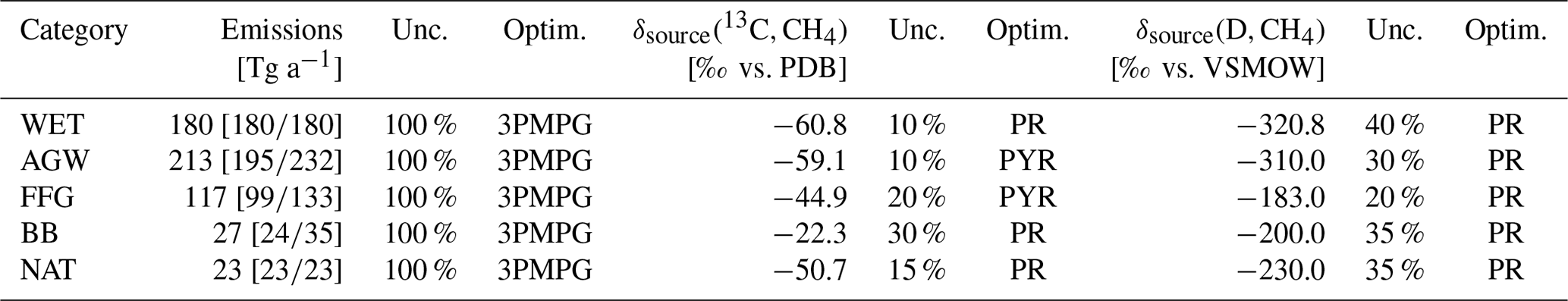
Emissions are optimized at the grid-cell scale (one scaling factor per grid cell). For each category, diagonal elements of the matrix B are filled with the variances set to 100 % of the square of the maximum of the prior emissions over the cell and its eight neighbors during each month. Spatial error correlations (off-diagonal elements) are prescribed using an e-folding correlation length of 500 km on land and 1000 km over the oceans, without any correlation between land and ocean grid points. No temporal error correlations are prescribed.
2.4 Prior source signatures and uncertainties
δsource(13C,CH4) values for each emission category are also optimized and therefore included in the control vector. Prior information is built using the references given in Table 3. When regional information could be found, regional source signature values were prescribed for 11 continental regions (see Fig. 1, lower-right panel) for each subcategory. Isotopic signatures for subcategories are flux-weighted averaged to create signatures for categories, which results in signatures that are grid-cell dependent, although signatures for subcategories are set constant within a continental region. Signatures for wetlands are the only ones prescribed at the grid-cell scale, following Ganesan et al. (2018). We optimize the source signatures at the regional scale rather than at the grid-cell scale to avoid substantial posterior differences between two adjacent grid cells. At present, there would not be enough data to corroborate, explain, or reject such differences. We therefore apply only one scaling factor per continental region and per category.
Livestock source signatures have likely been decreasing over time since the 1990s due to changes in the C3 C4 diet within the major livestock producing countries (Chang et al., 2019). Also, FFG regional source signatures can vary over time due to variations in the contributions from different sectors (coal, oil and gas) to the emissions of a specific region (Schwietzke et al., 2016; Feinberg et al., 2018). For AGW and FFG source signatures, we therefore optimize one scaling factor per year for each continental region. As for the other emission categories, only one scaling factor for the entire period and for each continental region is optimized. Error covariances are prescribed following the same methods as those applied to CH4 emissions.
As for δsource(D,CH4), we adopted global values suggested by Warwick et al. (2016) and in agreement with the intervals given by Röckmann et al. (2016). One exception is for WET sources, for which the boreal (−360 ‰) and tropical (−320 ‰) regions are differentiated. All values are summarized in Table 2. For each category and each continental region, only one scaling factor is optimized for the entire period.
Table 3Global flux-weighted values and references for δsource(13C,CH4) source signatures associated with the different emission categories and subcategories. Values for subcategories are taken from the literature and prescribed either globally (G), regionally (R, see Fig. 1, lower-right panel), or at the pixel scale (P). E19: Etiope et al. (2019); CH19: Chang et al. (2019); GA18: Ganesan et al. (2018); TH18: Thompson et al. (2018); SH17: Sherwood et al. (2017); SH16: Schwietzke et al. (2016); WA16: Warwick et al. (2016); ZA16: Zazzeri et al. (2016); TO12: Townsend-Small et al. (2012); KL10: Klevenhusen et al. (2010); BO06: Bousquet et al. (2006); BR01: Bréas et al. (2001); SA01: Sansone et al. (2001); CH00: Chanton et al. (2000); HO00: Holmes et al. (2000); CH99: Chanton et al. (1999); BE98: Bergamaschi et al. (1998); LE93: Levin et al. (1993).
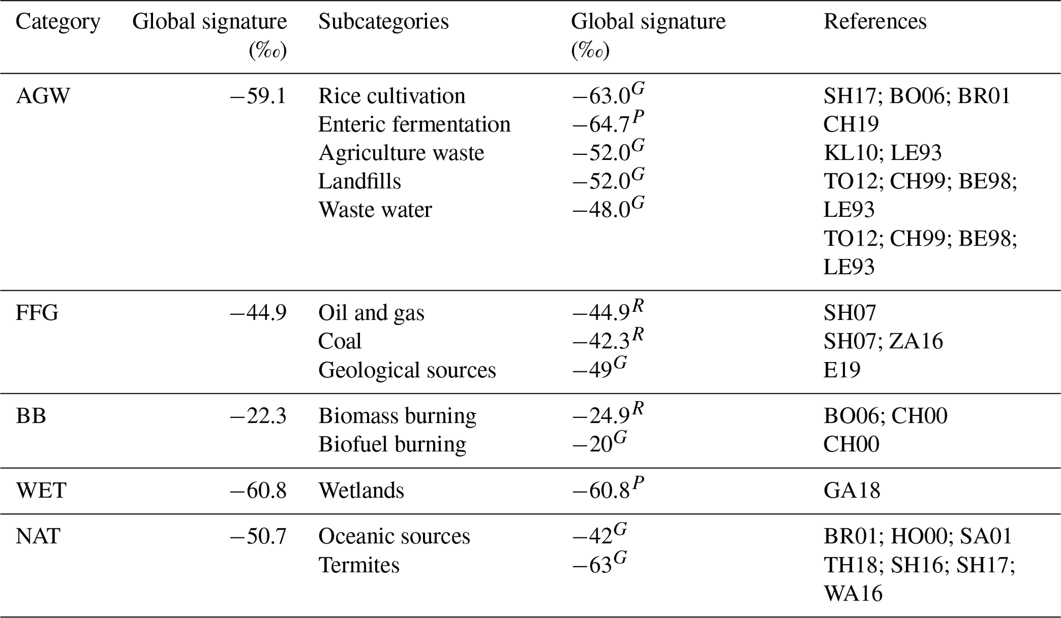
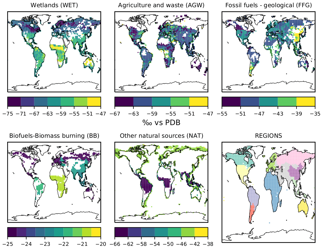
Figure 1Prior estimates of δsource(13C,CH4) isotopic signatures for each of the five emission categories averaged over the 1998–2018 period. The regions over which the values are optimized are shown in the lower-right panel. WET source signatures are dependent on the latitude, with more depleted values occurring in boreal regions than in tropical regions. BB source signatures are dependent on the vegetation (C3 C4). Burning C4 vegetation in tropical regions releases CH4 that is more 13C enriched than the CH4 released when burning C3 vegetation. The AGW source signature is dependent on the country/region and the C3 versus C4 livestock diet. FFG source signatures mainly depend on both the location and the contributions from coal, oil, gas and geological sources to the total FFG emissions of a specific country/region. For example, China's large 13C-enriched coal emissions greatly contribute to the FFG source signature in this region, which is notably 13C enriched compared to other regions.
δsource(13C,CH4) uncertainty values that are used to fill the diagonal elements of the matrix B are summarized in Table 2. These values have been chosen by compiling data from several studies (Sherwood et al., 2017; Ganesan et al., 2018; Feinberg et al., 2018; Zazzeri et al., 2016). The observed variability over the whole globe (standard deviation σ or minimum–maximum range) presented in these studies for each category is compiled and applied here as an uncertainty (1σ), thus adopting the same value for all regions. Note that for BB sources, Sherwood et al. (2017) indicates a global standard deviation of about 20 %. However, this value is not weighted by the proportion of C3 versus C4 vegetation. Therefore, we inflated this uncertainty to 30 % to account for the uncertainty in the type of vegetation. δsource(D,CH4) uncertainty values were derived from the minimum–maximum ranges suggested by Röckmann et al. (2016). We could have also used the standard deviation provided by Sherwood et al. (2017). However, as the amount of data for AGW, BB, WET and NAT source signatures is very low compared to the δsource(13C,CH4) values, we prefer to use larger uncertainties and examine whether the assimilation of δ(D,CH4) observations modifies the results. For future studies, additional δ(D,CH4) data to derive realistic regional estimates, especially for non-fossil sources, would be invaluable.
We acknowledge the fact that our methods are not perfect and that the prescribed regional uncertainties might be too large compared to the regional observed uncertainties that are currently estimated, especially for δsource(13C,CH4). As our inversion system is used for the first time over a time period exceeding 10 years, it is difficult to predict the influence of the setup on the results. As the time required to run an inversion is very high at the moment (see Sect. 2.9), we prefer to assess the behavior of this system in response to a simple (and probably slightly loose) setup and to estimate whether such uncertainties are small enough to help better constrain the CH4 budget. Additionally, source signature data representativeness is generally poor, owing in part to the small number of samples and the lack of data for several regions, particularly for non-fossil sources. It might therefore be challenging to derive a robust uncertainty using a data-driven approach for each region of the world. However, there is definitely room for improvement, and future work will build on the present work to improve this methodology and assess and prescribe better uncertainties.
Note that random uncertainties are only one side of the coin when it comes to uncertainties. Systematic uncertainties must also be investigated when using isotopic constraints. In particular, Oh et al. (2022) derived source signature maps for wetland sources that carry systematic uncertainties. Typically, inverse modelers address such uncertainties by conducting numerous inversions using parameters designed to account for these systematic errors. The high computational cost associated with our system prevents us from running a large number of inversions. Nevertheless, only one scaling factor is applied for each region and each category. Consequently, there is a strong regional correlation between random errors. To some degree, this approach enables the detection and correction of regional systematic errors by our system. It is important to note, however, that this correction does not rely on any existing sensitivity analysis (e.g., Lan et al., 2021; Basu et al., 2022), but rather uses solely the information provided by atmospheric isotopic observations.
2.5 Observations
2.5.1 Assimilated data
Our study uses observations from the NOAA Global Monitoring Laboratory (NOAA GML) Global Greenhouse Gas Reference Network. CH4 measurements are made by NOAA GML (Lan et al., 2022), and isotopic measurements are made at the Stable Isotope Laboratory at the Institute of Arctic and Alpine Research (INSTAAR) (White et al., 2021, 2016). This ensemble was selected to provide the largest number of consistent CH4 and isotopic data since 1998. Seventy-nine stations (four of which were mobile stations) provided CH4 measurements between 1998 and 2018 (not necessarily over the full period), 22 stations provided δ(13C,CH4) measurements between 1998 and 2018, and 15 stations provided δ(D,CH4) measurements between 2005 and 2010 (see Fig. 2). Missing CH4 instrumental errors are filled with the maximum value of this error at the station over the monitoring period. For δ(13C,CH4) and δ(D,CH4) measurements, missing instrumental errors are filled with a value of 0.1 ‰ and 3 ‰, respectively (Quay et al., 1999). Variances (diagonal elements) in the covariance matrix R are defined as the sum of the instrumental and model errors (variances). For each station and each year, we used the residual standard deviation (RSD) between the measurements and a fitting curve function as a proxy for the model error (Thanwerdas et al., 2022a; Locatelli et al., 2015; Bousquet et al., 2006). The fitting function includes three polynomial parameters (quadratic) and eight harmonic parameters, sine and cosine, as in Masarie and Tans (1995). We also remove outliers that are outside three times the residual standard deviation, as such extreme values cannot be reasonably reproduced at the horizontal grid resolution of LMDz. Typical values for observation errors are 20 nmol mol−1 for CH4, 0.3 ‰ for δ(13C,CH4) and 7 ‰ for δ(D,CH4).
2.5.2 Satellite data used for comparison
The Greenhouse Gases Observing Satellite (GOSAT), which carries a Fourier-transform spectrometer within its Thermal And Near-infrared Sensor for carbon Observation (TANSO-FTS) (Kuze et al., 2016), provides radiance measurements in a spectral band centered on a value close to 1.6 µm, in which CH4 has a high absorption capacity. The University of Leicester's retrieval algorithm is able to produce column-average dry air amount fractions of CH4 from these radiances. Although this quantity is commonly referred to with the symbol XCH4 in the existing literature, it is denoted here by because this is considered a more valid notation. We use version 9.0 of the GOSAT Proxy dataset provided by the University of Leicester (Parker et al., 2020) to evaluate the after the inversion process. To this end, vertical profiles simulated by LMDz-SACS are sampled at the observation location and time and convolved with the retrieval of the prior vertical profiles and column averaging kernels provided by the University of Leicester. Finally, within each grid cell, all the individual differences between the satellite observations and model outputs are averaged.
Satellite data are not assimilated here because inversions assimilating both satellite and surface data have not yet been performed with LMDz-SACS. Before using satellite data and isotope data together in an inversion, we need to rigorously assess the added value of satellite data without isotope constraints.
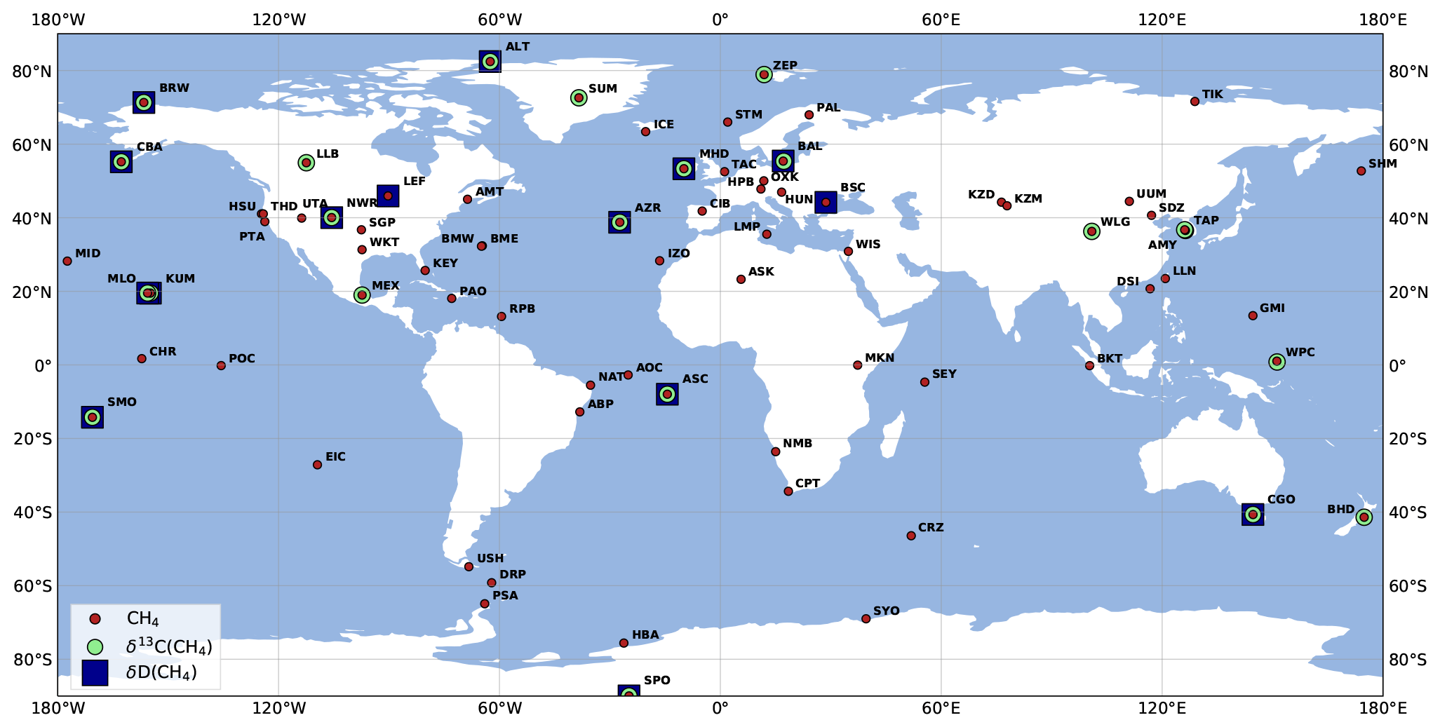
Figure 2Locations of surface CH4, δ(13C,CH4) and δ(D,CH4) stations in the NOAA GML network. Samples from several stations are retrieved and analyzed by INSTAAR to provide δ(13C,CH4) and δ(D,CH4) observations. More information about the stations can be found in Appendix A. Note that mobile stations (AOC, PAO, POC and WPC) are each indicated by a single point for clarity.
2.6 Initial conditions
To infer the initial CH4 and δ(13C,CH4) conditions for 1998, we run an inversion between 1988 and 1998 using the same prior emissions and isotopic signatures as that of INV_REF. We assimilate CH4 measurements from the NOAA GML network (56 stations) and δ(13C,CH4) measurements retrieved at five stations across the globe by the University of Washington (UW) between 1988 and 1996 (Quay et al., 1999; Bousquet et al., 2006), which we offset by 0.1 ‰ to account for measurement differences between INSTAAR and UW (Umezawa et al., 2018).
We also run a forward simulation from 1998–2010 to obtain a good spatial distribution of the δ(D,CH4) field and then apply a global offset to match the observed mean δ(D,CH4) value between 2005 and 2010. As we acknowledge that both methods are not perfect, considering the equilibration times of these isotopic compositions (Tans, 1997), we also prescribe large uncertainties in these initial conditions: 10 % for CH4, 3 % for δ(13C,CH4) and 20 % for δ(D,CH4). To optimize the initial conditions, the globe is regularly discretized using latitudinal and longitudinal bands. A step of 30∘ is applied to generate the bands, resulting in 6 × 12 = 72 regions. One scaling factor is optimized for each of these regions.
2.7 Description of the sensitivity tests
The reference inversion was first introduced in Sect. 2.2, and its setup is detailed in previous sections. Three sensitivity tests were conducted to investigate the influence of the setup of our system on posterior estimates when assimilating isotopic observations:
-
INV_CH4 is an inversion that only assimilates CH4 observations, not δ(13C,CH4) nor δ(D,CH4) observations, and thus only optimizes CH4 emissions for the five categories.
-
INV_DD assimilates CH4, δ(13C,CH4) and δ(D,CH4) observations and optimizes both δsource(13C,CH4) and δsource(D,CH4) source signatures. Note that δ(D,CH4) observations only span the period from 2005–2010, and therefore the full run cannot be fully constrained by this data.
-
INV_LOCKED is an inversion that assimilates CH4 and δ(13C,CH4) observations but does not optimize δ(13C,CH4) source signatures (fixed to prior values). This run considers source signatures fixed to prior values and thus investigates the influence of overconstrained isotopic signatures on posterior estimates.
We also investigate the influence of the OH interannual variability (IAV) on our results. The OH IAV in the troposphere is usually derived from inversions using CH3CCl3 constraints (Montzka et al., 2011; Rigby et al., 2017; Turner et al., 2017; Naus et al., 2019) or using global atmospheric chemistry–climate models (He et al., 2020; Dalsøren et al., 2016). CH3CCl3 inversion-based studies suggest a decrease in post-2005 OH after a peak in 2000–2002. By contrast, the chemistry modeling studies derive a post-2005 stabilization after a quasi-continuous increase between 1990 and 2005, consistent with the OH IAV estimated by LMDz-INCA (see Fig. 3). We therefore perform two more sensitivity tests:
-
INV_TURNER is designed to investigate the influence of the IAV on our results. We apply the IAV suggested by Turner et al. (2017) to the OH-INCA field. The associated OH field is named OH-TURNER, and its global concentrations decrease by 7 % between 2002 and 2014.
-
INV_FLATOH removes the IAV from our OH-INCA field by prescribing the concentrations for the year 2000 over the full period. The associated field is named OH-FLAT.
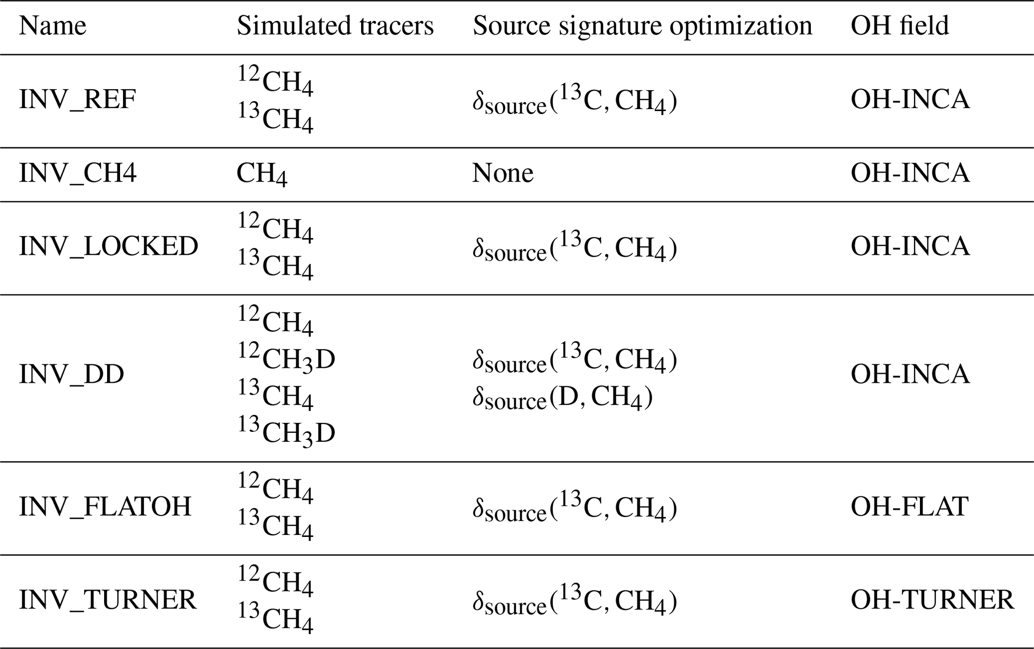
All the sensitivity tests are summarized in Table 4.
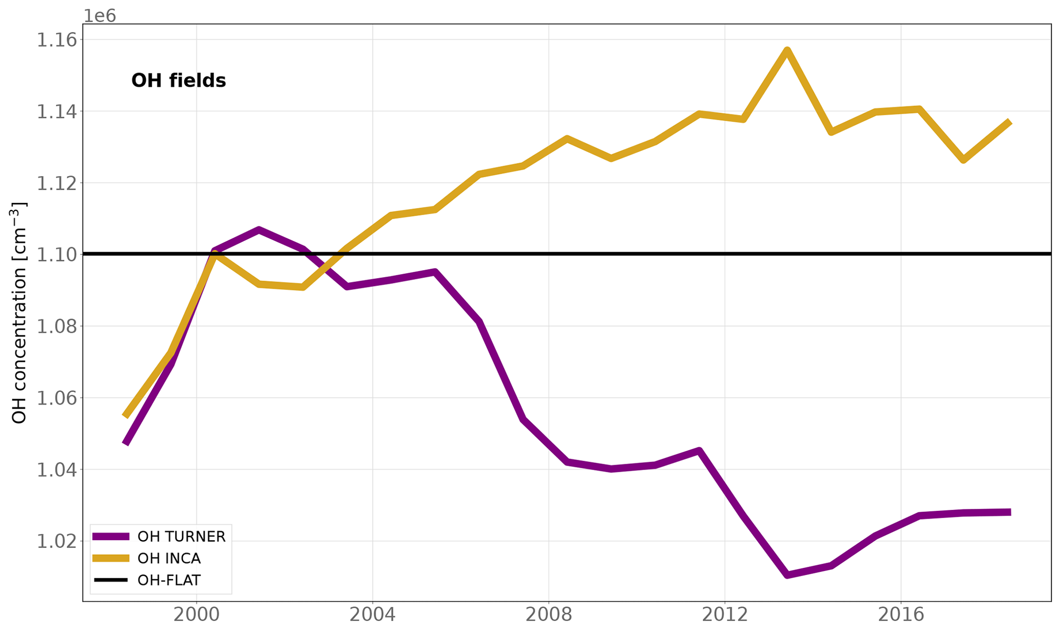
Figure 3Time series of the global volume-weighted tropospheric OH annual concentrations for the 1998–2018 period. OH-INCA was simulated by the LMDz-INCA chemistry model. OH-TURNER was obtained by applying the IAV from Turner et al. (2017) to the OH-INCA field. OH-FLAT has no interannual variability and concentrations are set equal to those of OH-INCA in 2000. In 1980, the OH-INCA mean concentration is very close to 10.0 × 105 cm−3, which was also taken as a reference value by Turner et al. (2017). This year is therefore taken as a reference to derive the anomalies.
2.8 Analysis period
Thanwerdas et al. (2022a) suggested that the results of the inversion should be discarded for the period up to 2–3 years after the beginning and the period 2–3 years before the end of the assimilation window. Although the term “spin-up” is not quite appropriate for the beginning of the window because the reason for discarding those results is slightly different, the outcome is still similar. The spin-up time, for an inversion, typically refers to a period at the beginning of the inversion when the errors in the assumed initial concentration field might influence the posterior fluxes. If the adopted spin-up period is too short, the inversion may fit the data by compensating for errors in the initial conditions with artificial emission adjustments. If the initial concentrations are also optimized, which is the case here, this effect can be reduced (Houweling et al., 2017). However, source signatures are optimized, and, for a certain period after the start of the inversion, it is easier for the system to optimize the initial δ(13C,CH4) fields than the source signatures to fit the δ(13C,CH4) data. Thanwerdas et al. (2022a) found that the optimized source signatures slowly move away from the prior value over time. After 2–3 years, the posterior value finally reaches a new and rather stable state. In other words, as the influence of the initial conditions on the isotopic composition decreases, the system prefers to optimize the source signatures, hence slowly reaching the posterior value. The equilibration time for δ(13C,CH4) and δ(D,CH4) is larger than the CH4 equilibration time (Tans, 1997), and therefore the signatures are more affected than the fluxes. For the end of the inversion, the reason for discarding the results is a lack of constraints, resulting in a slow return to the prior value. In this case, the use of the term “spin-down” is correct.
In addition, the strong 1997–1998 El Niño event leads to fire emission anomalies of about 20 Tg a−1 according to GFED4s data and studies (Bousquet et al., 2006; Langenfelds et al., 2002). Similarly, the following 1999–2000 La Niña event produced a wetland emission anomaly that persisted until 2002 (Zhang et al., 2018). Finally, OH concentrations were also likely affected by this El Niño–Southern Oscillation (ENSO) phase (Zhao et al., 2020a). We therefore only analyze the results of the 2002–2014 period to limit the consequences of these effects. This period of time is large enough to explain the variations that caused the post-2007 CH4 renewed growth and the associated δ(13C,CH4) shift to more negative values.
2.9 Computational aspects
The same convergence criterion was used for all inversions in order to ensure consistency between the results. The minimization process was stopped when at least 35 iterations (forward + adjoint runs) had been performed and the gradient norm ratio had fallen below 1 % of its initial value for four successive iterations.
A similar number of iterations (approx. 40) were necessary for all sensitivity tests. About 260 CPU hours were necessary to run a single iteration on LSCE (Laboratoire des Sciences du Climat et de l'Environnement) computational clusters consisting of Intel® Xeon® Gold 5317 central processing units (CPUs) with a frequency of 3.00 GHz. For this work, eight CPUs were run in parallel, resulting in a runtime of 32.5 h for a single iteration. More CPUs could not increase the overall performance because of some I/O (input/output) limitations of our offline model. With only one tracer to simulate, INV_CH4 therefore required about 2 months to reach the convergence criterion. Because the runtime is proportional to the number of simulated tracers, double this runtime was needed for the other inversions (two tracers), except for INV_DD, which required four times this runtime (four tracers).
While the number of CPU hours needed for these complex inversions remains reasonable, the overall runtime is excessive. It is therefore an important limitation of our system. Further developments of parallelization methods are being implemented to enable a significant reduction of the computational cost (e.g., Chevallier, 2013). This method consists of breaking down the full assimilation window into multiple sub-windows and running smaller inversions in parallel for each sub-window. If source signatures remain constant, we expect the results to closely resemble those of a longer-term window inversion. Conversely, if source signatures are optimized, the influence of the initial conditions on the atmospheric isotopic composition might persist over a time that is larger than the length of the sub-window. In this case, source signatures might remain unchanged and the results could be impacted. Therefore, it is crucial to rigorously validate this parallelization method before interpreting its outcomes.
In this section, we first verify the quality of the model's fit to the constraining observations and evaluate it against independent data (Sects. 3.1 and 3.2). After this, we examine the posterior estimates of our reference inversion for emissions and source signatures and compare them to prior estimates (Sects. 3.3 and 3.4). Subsequently, we attribute the CH4 increase and downward shift in δ(13C,CH4) post-2007 to changes in CH4 emissions and source signatures (Sects. 3.5 and 3.6). Finally, we analyze the sensitivity of our results to setup modifications (Sects. 3.7 and 3.8).
3.1 Model–observation agreement
Before analyzing the optimized emissions and source signatures, we verify the quality of the model's fit to the constraining observations and evaluate it against independent data. A good fit shows that the system is operational over long time periods and that posterior emissions and source signatures are consistent with the observed state of the atmosphere.
The observed globally averaged CH4 amount fraction as well as the observed globally averaged δ(13C,CH4) isotopic composition at the surface are well captured by all the posterior simulations (see Fig. 4b, d). INV_REF shows a Pearson's moment correlation coefficient r of 0.994 for CH4 (RMSE is 2.8 nmol mol−1) and 0.936 for δ(13C,CH4) (RMSE is 0.04 ‰). The posterior simulation therefore captures the observations much better than the prior simulation does (RMSEs of 71.2 nmol mol−1 and 1.44 ‰, respectively). The inversion that best captures the δ(13C,CH4) isotopic composition is INV_DD, with a RMSE of 0.02 ‰. This shows that assimilating δ(D,CH4) observations slightly increases the agreement with isotopic observations without performing additional iterations.
The 2002–2007 δ(13C,CH4) stabilization is well reproduced by the model in INV_REF, with a mean RMSE of 0.02 ‰ over the period. However, the post-2007 trend is not as consistent (0.05 ‰), mainly due to an overestimation of the decreasing rate (0.03 ‰ a−1 against 0.02 ‰ a−1). The simulated δ(13C,CH4) seasonal cycle amplitude is also slightly smaller than the observed one (0.12 ‰ against 0.14 ‰, respectively), although the two signals are well phased. Note that our results are, however, still within the prescribed observation uncertainty range.
For the sake of completeness, we also provide a comparison between δ(D,CH4) observations and prior and posterior simulations from INV_DD in Appendix B (Fig. B1). After the inversion, simulations capture the observed δ(D,CH4) data much better, reducing the RMSE from 9.3 ‰ to 1.2 ‰. Although the δ(D,CH4) data are much more limited than the δ(13C,CH4) data, linear regressions indicate a small negative trend (−0.23 ± 0.12 ‰ a−1) between 2005 and 2009. Additionally, the trend is positive between 2005 and 2007 (+0.86 ± 0.42 ‰ a−1) and negative between 2007 and 2009 (−0.47 ± 0.25 ‰ a−1). This shows that δ(D,CH4) observations might also carry some information about the renewed growth of CH4 post-2007.
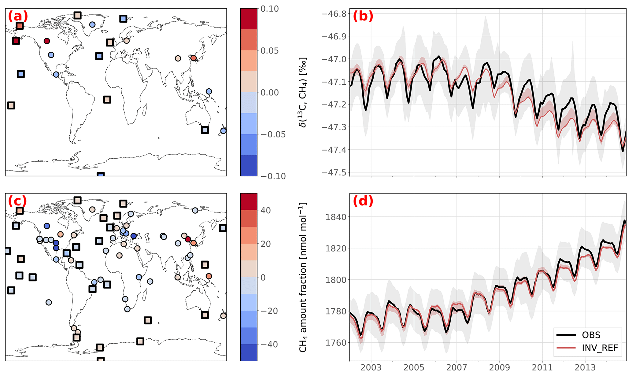
Figure 4Posterior agreement between INV_REF and assimilated observations. Panels (a) and (c) show the posterior CH4 and δ(13C,CH4) biases at the surface stations over the 2002–2014 period. Marine boundary layer stations are indicated by squares rather than circles. Panels (b) and (d) show the observed (solid black line) and simulated (solid red line) globally averaged trends in CH4 and δ(13C,CH4). The red-shaded area shows the minimum and maximum values over the sensitivity tests. The gray-shaded area shows the standard error of the globally averaged observed trend. This error is based on the error prescribed in the matrix R, i.e., the sum of the measurement and model errors. The same figure with prior data is provided in Appendix B (Fig. B2).
The model–observation agreement varies across the stations for both CH4 and δ(13C,CH4) (see Fig. 4a and c). CH4 at marine boundary layer (MBL) stations (i.e., where site samples consist mainly of well-mixed MBL air) is very well reproduced by the model (mean RMSE of 17.7 nmol mol−1 and mean bias of −1.87 nmol mol−1). The model has more difficulties in simulating amount fractions at several polluted stations, such as Lac La Biche, Canada (54.95∘ N, 112.45∘ W), Shangdianzi, People's Republic of China (40.65∘ N, 117.12∘ E), Anmyeon-do, Republic of Korea (36.54∘ N, 126.33∘ E), or the Southern Great Plains, United States (36.62∘ N, 97.48∘ W), presumably owing to transport errors, representation errors and/or inaccurate estimates of CH4 prior fluxes around these stations. The δ(13C,CH4) at MBL stations is generally correctly simulated, with RMSEs of 0.2 ‰–0.3 ‰, comparable to the prescribed uncertainties. However, posterior simulations slightly overestimate δ(13C,CH4) in Northern America and underestimate it in Central America and temperate North America. This suggests an over- and underestimation of flux-weighted source signatures in these regions, respectively. This is further investigated in Sect. 3.4.
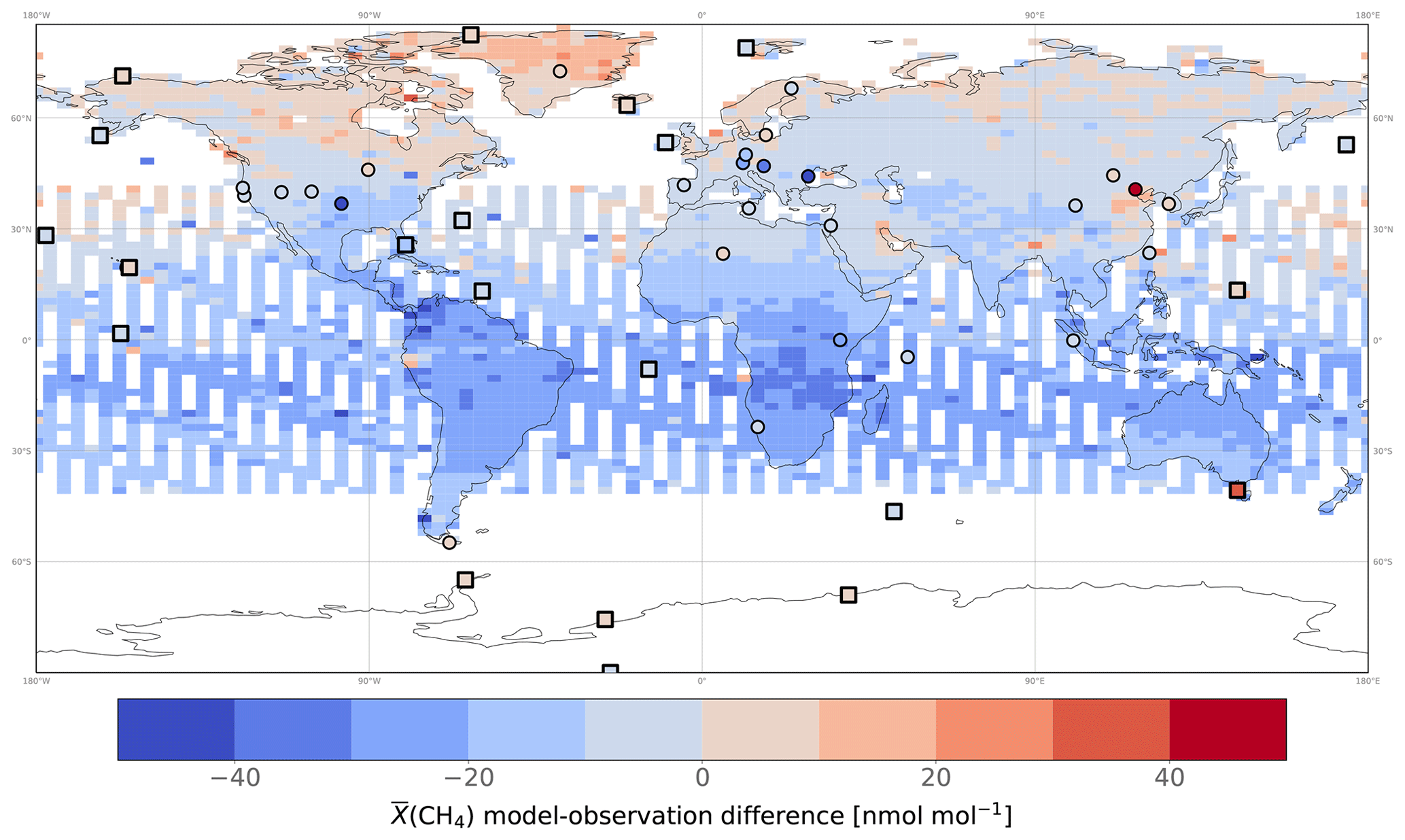
Figure 5Mean posterior model–observation differences in averaged over 2010 and gridded at the model resolution. Model outputs were obtained using the posterior estimates of INV_REF and by applying the averaging kernels provided by the University of Leicester. Model–observation differences at assimilated surface stations are also displayed for comparison. We acknowledge that the temporal sampling by surface stations is not identical to that of satellite data, which might affect the comparison. To limit this effect, only stations providing at least one observation for each month of 2010 are displayed to reduce the seasonal influence. MBL stations are indicated by squares rather than circles.
3.2 Comparison of model-optimized with satellite-derived column-average CH4 amount fractions
For comparison, we performed one forward simulation with posterior fluxes obtained with INV_REF to compare our simulated to independent (i.e., not assimilated) satellite observations in 2010 and evaluate the optimized atmosphere (see Fig. 5). The posterior mean bias is −13.0 nmol mol−1, indicating that the GOSAT observations are higher overall than our optimized , even after the inversion. Further analysis reveals that the mean bias (−17.5 nmol mol−1) in the tropics (30∘ S–30∘ N) is larger in absolute value than the bias in the northern mid-latitudes (30–60∘ N; −5.7 nmol mol−1) or in the northern high latitudes (60–90∘ N; +3.0 nmol mol−1). Parker et al. (2020) also reported observing a negative mean bias (−6.55 nmol mol−1) when using the TM5 model and posterior estimates deduced from a surface-based inversion. Similar to ours, the TM5 biases were mostly located in the tropics and northern mid-latitudes. Ostler et al. (2016) reported that model errors when simulating stratospheric CH4 amount fractions could contribute to the bias. However, they did not find a strong improvement for LMDz and TM5 when replacing model simulations with MIPAS (Michelson Interferometer for Passive Atmospheric Sounding) stratospheric CH4. While this suggests that the biases in the GOSAT simulation presented here are probably not caused by stratospheric discrepancies, it is important to note that the same authors conclude that current satellite measurements of stratospheric CH4 may lack the precision necessary to eliminate these biases.
If we assume that the biases are solely the result of emission discrepancies, our findings indicate that the estimated tropical posterior emissions from our inversions might still be underestimated. Although posterior biases are lower at the surface stations in the tropics (the mean value is −5.3 nmol mol−1), the number of stations is limited in this area, especially in South America and Central Africa. Saunois et al. (2020), using configurations similar to ours but no isotopic constraints, found that differences between emissions from GOSAT-based and surface-based inversions mainly occurred in the tropical regions.
The in situ-only and the GOSAT-only inversions performed by Lu et al. (2021) provided 113 and 212 independent pieces of information, respectively, highlighting that additional constraints can be gained using satellite data. As tropical fluxes likely had a significant influence on the renewed increase of CH4 around 2007, it would be interesting to assimilate satellite observations to increase the constraints in the tropics. Furthermore, jointly assimilating satellite observations and isotopic observations might be valuable because tropical emissions largely dominate the total global release of CH4. Consequently, a change in tropical emissions might influence the global flux-weighted source signature and impact the results of an inversion performed with isotopic constraints. Our system is capable of performing such a joint assimilation; however, since we are analyzing the influence of adding isotope constraints here, we prefer to assimilate only surface data as a first step.
3.3 Posterior–prior emission differences
Global emissions are estimated by INV_REF at 590 Tg a−1 when averaged over the 2002–2014 period, which is larger than prior estimates by 28 Tg a−1 (see Fig. 7). This change mainly arises from increases in Asia (+15 Tg a−1), Central and South America (+6 Tg a−1), and Africa (+3 Tg a−1). About 50 % and 25 % of the increase in Asia is due to the AGW and FFG categories, respectively, suggesting that the prior estimates in EDGARv4.3.2 for these regions are underestimates. However, global emissions estimated by inverse modeling are strongly dependent on the chemical loss prescribed in the CTM. OH is responsible for most of this loss and therefore the prescribed OH field greatly influences the results of the inversion. In particular, Zhao et al. (2020b) showed that a 1 × 105 cm−3 increase in prescribed OH concentrations leads to an increase in CH4 global posterior emissions of 40 Tg a−1. Here, we are more interested in the trends in various CH4 emission categories and their contributions to the total emissions. Therefore, we have only used a single OH field with several trends. The influences of the trends on the dedicated inversions are further discussed in Sect. 3.8.
The posterior global distribution of emissions across the individual categories is only slightly different from the prior one (see Fig. 6). Relative posterior–prior emission differences averaged over 2002–2014 are larger for WET (+7 %) than for AGW (+4 %), FFG (+6 %) or BB (+5 %). The increase in WET emissions is mainly located in the Amazon basin (43 %) and is responsible for a small shift in the WET contribution to the total emissions (from 32.1 % to 32.6 %), which is offset by a similar reduction in the AGW contribution (from 37.9 % to 37.4 %). The tropics (90∘ S–30∘ N), the northern mid-latitudes (30–60∘ N) and the high latitudes contribute about 60 %, 35 % and 5 % to the global emissions, respectively. Apart from a small reduction in the contribution from high latitudes, the latitudinal distributions of emissions are not modified.
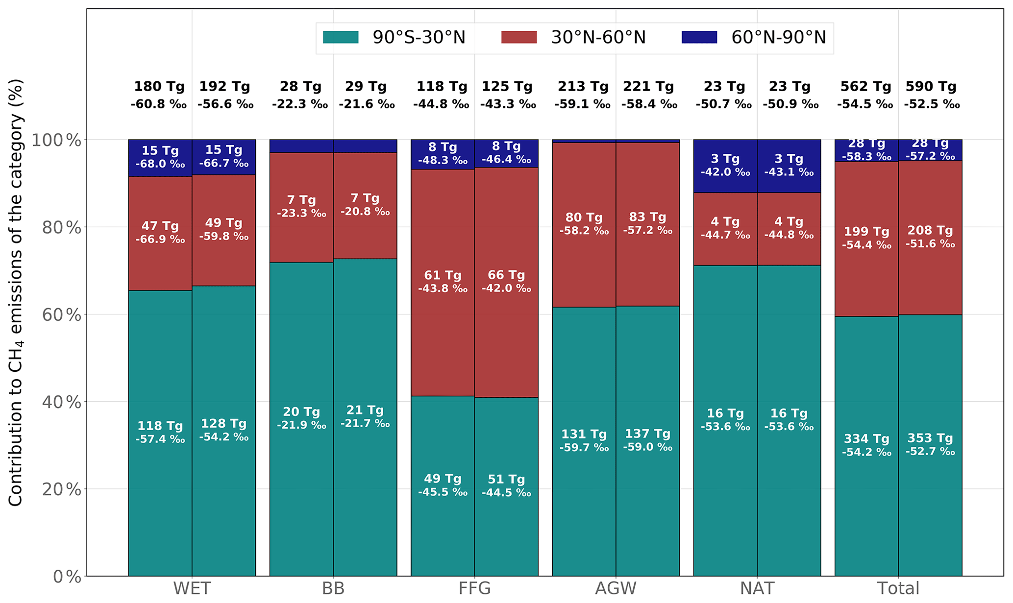
Figure 6Prior (left) and posterior (right) contributions from three latitudinal regions to global CH4 emissions for each emission category. Posterior emissions are taken from INV_REF. The latitudinal bands are (1) the tropics (90∘ S–30∘ N), (2) the northern mid-latitudes (30–60∘ N) and (3) the high latitudes (60–90∘ N). Emissions and source signatures for each region and category are given in the associated bars. The total emissions and global source signatures for each category are given on the top of each bar.
3.4 Posterior–prior source signature differences
Global and regional source isotopic signatures are calculated using a flux-weighted average to account for the global and regional source mixture, respectively. Therefore, they may be modified by the system due to a source mixture change and/or a source signature change in a specific region.
The inversion system shifts the global source signature considerably upward from −54.5 ‰ to −52.5 ‰ (see Fig. 6). The global signature is highly constrained by the fractionation coefficients and the concentrations of radicals (OH, Cl and O1D) prescribed in the CTM. Our posterior global source signature is higher (less negative) compared to other estimates (Sherwood et al., 2017; Rigby et al., 2017; Schaefer et al., 2016), mainly because we chose to prescribe Cl concentrations and an OH fractionation that are at the low ends of the existing ranges. Each additional percent of oxidation caused by the prescribed Cl sink would lead to a drop in the global source signature of about 0.5 ‰ (Thanwerdas et al., 2022b; Strode et al., 2020). Using other recent estimates of Cl tropospheric concentrations (see Sect. 2.1), our posterior global source signature would range between −54.5 ‰ and −52.5 ‰. In addition, the application of the fractionation value derived by Cantrell et al. (1990) instead of that derived by Saueressig et al. (2001) would likely shift the global signature downward by another 1.5 ‰.
AGW, BB and FFG source signatures are shifted upward by 0.7 ‰, 0.7 ‰ and 1.3 ‰, respectively. Most notably, the posterior global flux-weighted WET signature is considerably higher (−56.6 ‰) than the prior estimate (−60.8 ‰) (see Fig. 6) with regard to recent estimates (Sherwood et al., 2017; Feinberg et al., 2018; Ganesan et al., 2018; Oh et al., 2022). This global shift mainly arises from upward regional source signature shifts in the tropics (+3.2 ‰) and in the northern mid-latitudes (+7.1 ‰), which together contribute 97 % of the posterior–prior global WET isotopic signature difference. The remaining contribution is due to an increase in the contribution from tropical WET emissions. Our posterior global estimate of the WET source signature strongly disagrees with the recent estimates. In Appendix B, Fig. B3 compares our prior and posterior signatures to observations from Supplement Data 1 provided by Oh et al. (2022). Overall, prior estimates show a better agreement with observations than posterior estimates. This poor agreement suggests that prescribed uncertainties might be too large (at least for WET) and supports the idea that the system yields an important adjustment of the WET signature in order to keep fossil/microbial flux partitioning unchanged. Notably, the isotopic signature in Canada is shifted upward from −70.0 ‰ (prior) to −59.4 ‰ (posterior), whereas that of Russia is shifted downward from −68.7 ‰ to −73.8 ‰. Although this demonstrates that the system is capable of applying offsets with different signs across different regions, it also appears to be unphysical, as the processes driving the source signatures in these high-latitude regions are similar (Ganesan et al., 2018; Oh et al., 2022). Nevertheless, the number of observations of WET source signatures is small and local uncertainties are considerable, especially in the tropics, where emissions from WET are the largest and where our system applies the most impactful adjustment. It is therefore difficult to invalidate the posterior adjustment. Further investigation, including a better assessment and prescription of the random and systematic uncertainties, is needed.
Figures B4 and B5 in Appendix B show the full temporal variations for the prior and posterior source signatures. For FF, high variations indicate a change in activities associated with fossil fuel extraction, e.g., switching from one location with a specific signature to another, transitioning from one fuel type (oil, gas, coal) to another, or a combination of both. For example, the substantial shift that occurred around 2009 in the United States was caused by a large increase in emissions from the extraction of natural gas. As we chose not to prescribe temporal error correlations between different years, the system is free to optimize each year independently to better fit δ(13C,CH4) observations. For certain continental regions, such as Africa, temperate Asia, or South Asia, the interannual variability of the source signature adjustments is large and rather unrealistic, especially when compared to the emission adjustments in the same regions (see Fig. 7). It is unlikely that these changes occurred without detectable changes in emissions in the same areas, especially for temperate Asia, which exhibits larger emissions from FF than in the United States. These results suggest the need to prescribe yearly temporal error correlations to dampen this artificial interannual variability. However, the example from the United States also indicates that large changes can occur, and it is reasonable to assume, considering the lack of isotopic data, that the prior data might not contain any information about potential substantial changes. Therefore, while implementing stronger temporal correlations could be a way to mitigate unrealistic interannual variability for this category, it diminishes the likelihood of detecting such changes that remain undetected by the prior data. Nevertheless, it might be sufficient to reduce the prescribed uncertainties in the source signatures in order to balance out the pressure applied by the system on the emissions and the source signatures. Overall, the same reasoning applies to AGW, although there is no evidence from the prior data that AGW source signatures can change as rapidly as those of FF. Due to the scarcity of existing data on the temporal variability of source signatures, designing a data-driven methodology to estimate potential temporal correlations, especially at the regional scale, remains highly challenging. Investigating the correlations that the system creates between the uncertainties associated with source signatures and fluxes could offer a promising avenue for extending the analysis. Due to the high computational cost of an inversion performed with our inversion system, it is impossible to derive robust posterior uncertainties. This impossibility is a major drawback, and additional studies with this system cannot be performed in the future without tackling this issue.
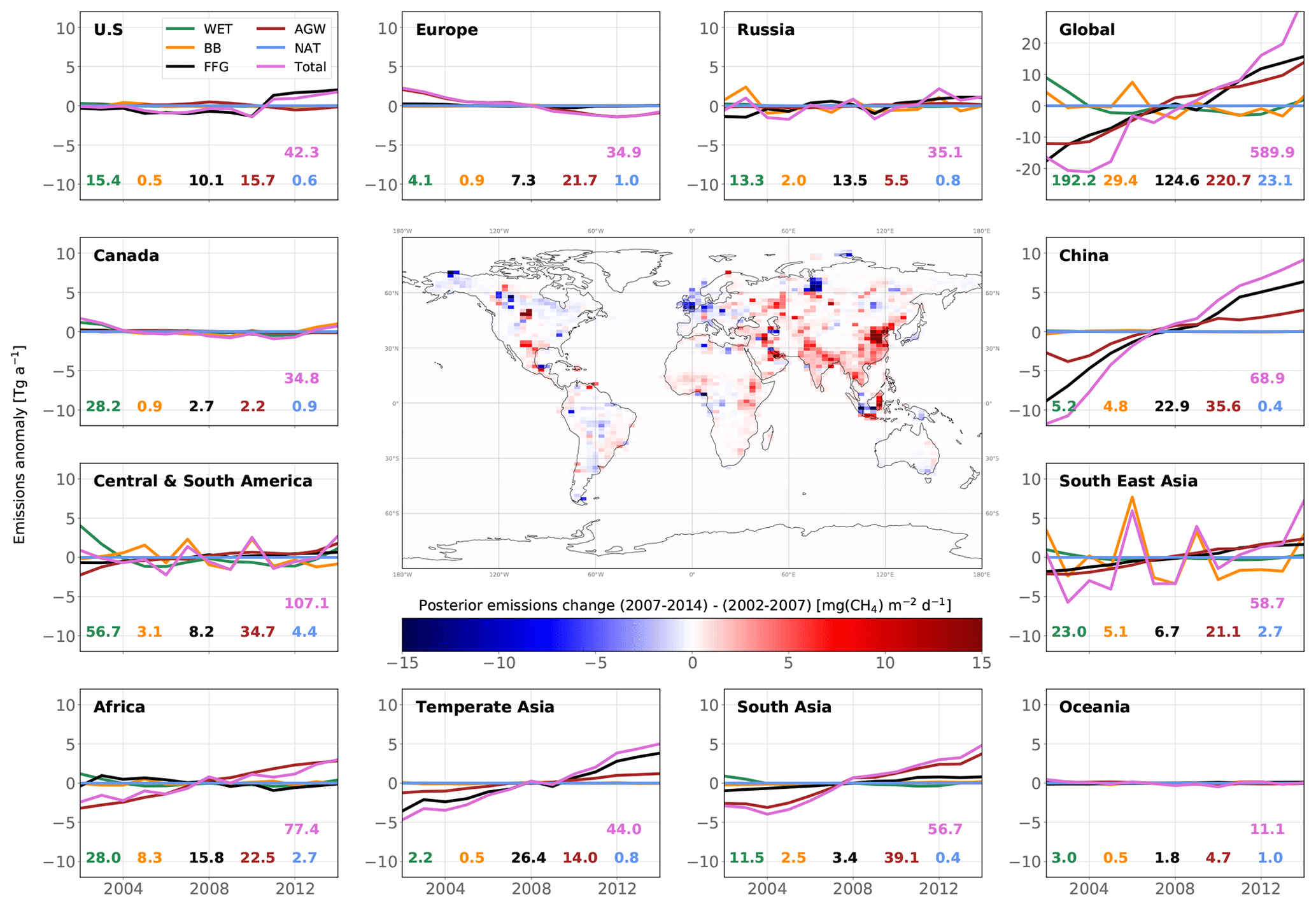
Figure 7Map of changes in posterior emissions from INV_REF between 2002–2007 and 2007–2014 (center panel) and time series of posterior emission estimates from INV_REF for multiple regions and all categories (panels around the map). For each panel, the time series show anomalies around the 2002–2014 mean value. For each category in each panel, the associated mean value is displayed in the same color as the solid line. The units of the variations and means are Tg a−1. The design of the figure is inspired by Fig. 1 in Chandra et al. (2021).
3.5 Attribution of the post-2007 CH4 increase
We now present trend results comparing the time periods before (2002–2007) and after (2007–2014) the renewed increase. Posterior global emissions show a net increase of 24.0 Tg a−1 (see Fig. 7). This occurred in most of the regions aside from Europe (−1.8 Tg a−1), Canada (−0.7 Tg a−1) and Oceania (−0.2 Tg a−1). China, South Asia (mainly India), temperate Asia, Southeast Asia and Africa accounted for 40 %, 18 %, 18 %, 10 % and 9 % of the associated positive increase (+26.7 Tg a−1), respectively. These results are consistent with prior information that estimated a rise of 27.5 Tg a−1. The large contribution from China to the global increase since 2002 agrees well with the regional estimate (40 %) from Thompson et al. (2015). We also estimate that Central and South America did not contribute to the renewed growth, in contrast with Chandra et al. (2021), who suggest a large contribution from Brazil (11.5 %) to the increase in global emissions. In this region, we find that small increases in AGW emissions (+1.4 Tg a−1) and FFG emissions (+0.7 Tg a−1) are offset by decreases in WET emissions (−0.8 Tg a−1) and BB emissions (−0.8 Tg a−1).
Global AGW emissions increased by 14.2 Tg a−1 between 2002–2007 and 2007–2014. Europe is the only region where these emissions substantially decreased (−1.7 Tg a−1). 80 % of the net AGW increase occurred in Asia, and the rest occurred in Africa and South America. FFG emissions increased by 14.9 Tg a−1, with 50 % of this increase occurring in China. These emissions notably decreased in Africa (−0.7 Tg a−1), Europe (−0.2 Tg a−1) and Canada (−0.1 Tg a−1). By contrast, WET emissions decreased by 2.4 Tg a−1, with 71 % of the net decrease located in Central and South America (33 %), Canada (25 %), and Africa (13 %). BB emissions also decreased by 2.7 Tg a−1, mainly due to decreases in Southeast Asia (55 % of the net decrease) and South America (24 %). Note that the analysis period does not include the 2015 El Niño event.
Our results therefore suggest that the renewed CH4 growth post-2007 (until 2014) was equally and mainly driven by increases in global AGW (49 %) and FFG (51 %) emissions. The decreases in global WET and BB emissions as well as the increase in global OH concentrations partially balanced this renewed growth. These findings are in partial agreement with recent studies (Chandra et al., 2021; Jackson et al., 2020; Thompson et al., 2018; Saunois et al., 2017), although only Jackson et al. (2020) explained the renewed growth with equal contributions from the AGW and FFG categories. The small decrease in BB emissions is consistent with other estimates (Thompson et al., 2018; Worden et al., 2017), but the decrease in WET emissions does not agree with recent findings that suggest either a constant trend or a positive trend (Chandra et al., 2021; Zhang et al., 2018; McNorton et al., 2018; Poulter et al., 2017; Bader et al., 2017).
However, posterior global WET emissions show negative anomalies between 1998 and 1999 and positive anomalies between 1999 and 2004. These anomalies are mainly located in South America, where about 30 % of WET emissions originate. Zhang et al. (2018) suggested that the 1998–2000 ENSO (El Niño–Southern Oscillation) caused negative anomalies in WET emissions between 1998 and 2000 because of El Niño and subsequent positive anomalies between 2000 and 2002 because of La Niña. The fact that positive anomalies persist until 2004 rather than 2002 in our posterior emissions cannot be easily explained. Also, the positive anomalies last 4–5 years in total, which is not consistent with the 2–3 years inferred by Zhang et al. (2018). As AGW emissions are also large in South America, the inversion system might be wrongly attributing large but decreasing emissions between 2002 and 2004 to WET emissions rather than AGW emissions. If the period 2002–2004, which exhibits large positive anomalies, is discarded, we find a small increase of 0.3 Tg a−1 in global WET emissions between 2004–2007 and 2007–2014, which is more consistent with the studies mentioned before.
3.6 Attribution of the post-2007 downward shift in δ(13C,CH4)
The posterior global flux-weighted δsource(13C,CH4) decreased from −52.1 ‰ in 2002 to −53.1 ‰ in 2010 and then experienced an upturn to −52.5 ‰ in 2012–2014. Notably, between 2007 and 2010, the decline in the source signature was rapid (−0.2 ‰ a−1), propagating into the atmosphere and contributing to the similar trend that appears in the observed globally averaged δ(13C,CH4). The subsequent increase after 2012 led to a stabilization of the associated atmospheric signal.
Between 2002–2007 and 2007–2014, all regional isotopic signatures were shifted downward (about −0.5 ‰ over the globe), except in China (+0.6 ‰). This is mainly explained by an increase in emissions from 13C-depleted sources in most of the regions but also by a decrease in emissions from 13C-enriched sources and a decrease in AGW and FFG source signatures.
Additionally, we use a simple mathematical framework to attribute the shift in the global flux-weighted signature to the different emission categories. Here, denotes the global flux-weighted δsource(13C,CH4). A first-order estimate of is given by
where fi denotes the global CH4 emissions from a specific category, N is the number of emission categories (five here), is the total CH4 emissions, and is the contribution from each category to the total emissions. A small variation in the global flux-weighted source signature, , can therefore be calculated using the derivatives dδi and dfi:
with
Using this simplified linear relationship, we find that the 0.34 ‰ decrease in (see Fig. 8) between 2002–2007 and 2007–2014 was due to
-
a decrease in the global AGW source signature (resulting in a shift in of −0.22 ‰),
-
a small decrease in BB emissions (resulting in a shift in of −0.15 ‰),
-
a large increase in AGW emissions (resulting in a shift in of −0.14 ‰),
-
a decrease in the FFG isotopic signature (resulting in a shift in of −0.09 ‰).
This decrease is partially offset by
-
a large increase in FFG emissions (resulting in a shift in of +0.24 ‰),
-
a small decrease in wetland emissions (resulting in a shift in of +0.02 ‰).
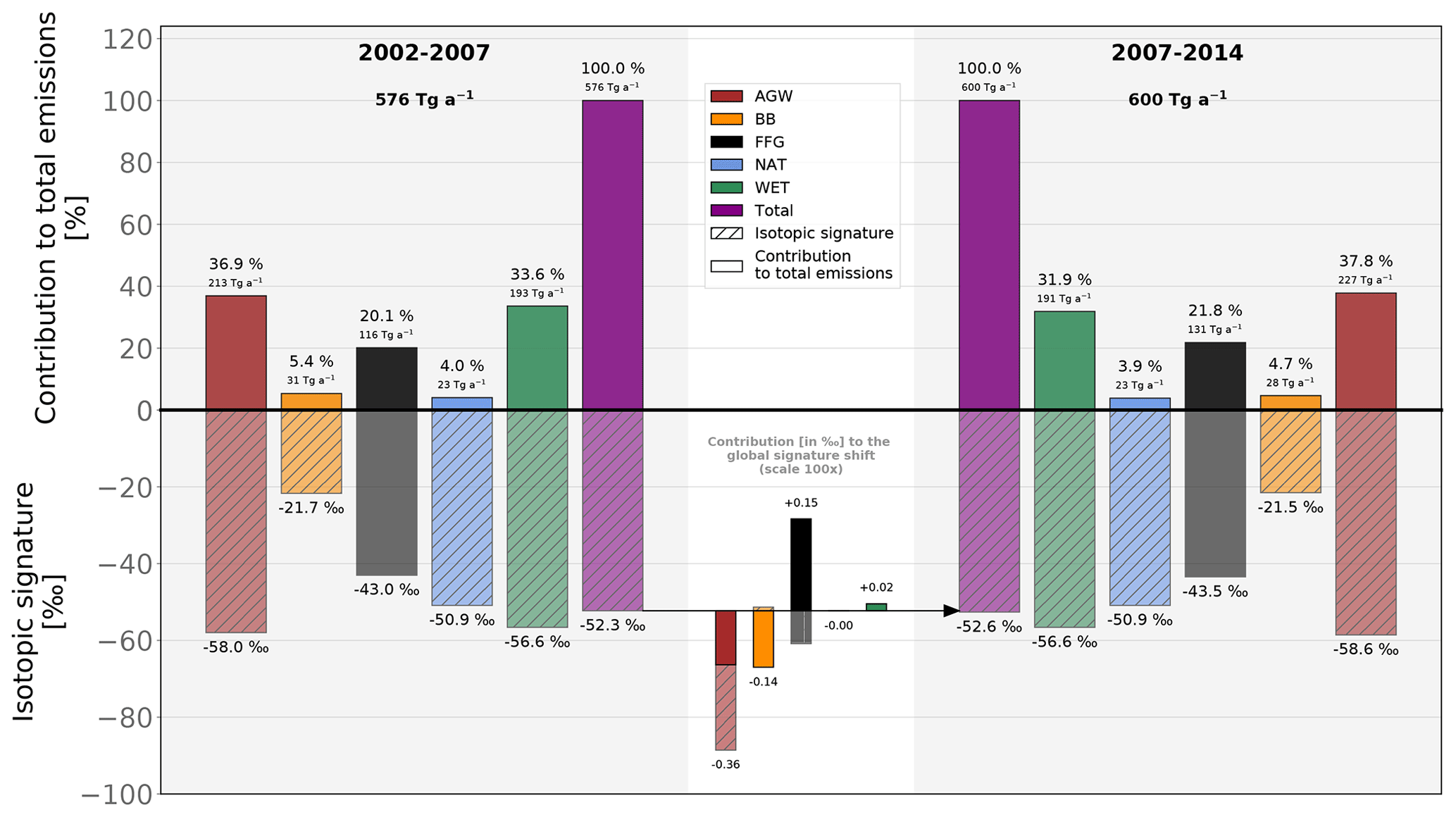
Figure 8Contributions of the changes in CH4 emissions and δsource(13C,CH4) source isotopic signatures to the global source signature shift between 2002–2007 (left side) and 2007–2014 (right side) in INV_REF. The upper part of the figure shows the contributions from the individual emission categories to the total emissions. Associated bars are non-transparent and non-hashed. Percentages and emissions are displayed on top of the bars. The lower part of the figure shows the isotopic signatures of each category. Associated bars are slightly transparent and hashed. The lower center with a white background shows the contributions from changes in emissions (non-transparent and non-hashed) and source isotopic signatures (slightly transparent and hashed) to the total source signature shift (−0.34 ‰) between the two periods. This part is magnified (×100) for clarity. Results from the other sensitivity tests are given in Table 5.
Table 5Upper part of the table: changes in CH4 emissions (emi.) and isotopic signatures (sign.) between 2002–2007 and 2007–2014 for each emission category and each sensitivity test. Lower part of the table: contributions from changes in emissions and isotopic signatures to the global flux-weighted source signature () shift between 2002–2007 and 2007–2014 for each emission category and each sensitivity test.
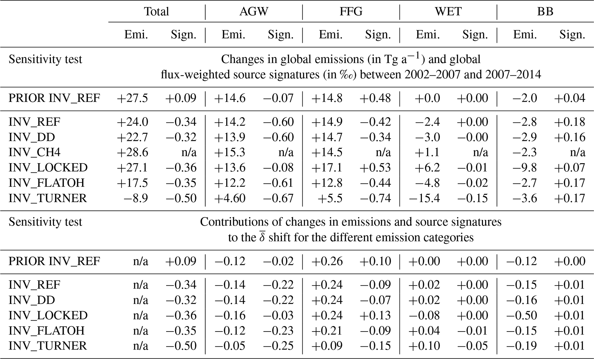
n/a: not applicable.
3.7 Sensitivity of the results to isotopic constraints
The reference inversion assimilates both CH4 and δ(13C,CH4). To quantify the impact of assimilating δ(13C,CH4) data, INV_CH4 assimilates CH4 observations only and does not simulate the isotopic composition. Differences between INV_REF and INV_CH4 therefore provide insight into the influence of the isotopic constraint. Notably, these two inversions show similar results for CH4 emissions. As both inversions are constrained by the same global sink, global emissions estimated by INV_CH4 are only 0.3 Tg a−1 lower on average over the 2002–2014 period. Tropical emissions are increased compared to INV_REF, and the contribution from tropical emissions to the total emissions is shifted from 59.8 % to 60.3 % (+2.5 Tg a−1), mainly due to an increase in WET tropical emissions (+1.6 Tg a−1), which is offset by decreases in the northern mid-latitudes (−1.2 Tg a−1) and high latitudes (−0.2 Tg a−1). WET emissions increase by 1.1 Tg a−1 in INV_CH4 between 2002–2007 and 2007–2014 (Table 5) instead of decreasing in INV_REF. The increases in AGW, FFG and WET emissions contribute 50 %, 47 % and 3 % of the post-2007 renewed growth, respectively, and are therefore slightly different from the results of INV_REF. To summarize, adding the isotopic constraint (INV_REF as compared to INV_CH4) slightly decreases the contribution from tropical emissions to global emissions, removes a very small contribution from WET emissions to the post-2007 renewed growth, and slightly changes the contributions from emission increases to the post-2007 renewed growth.
Differences between INV_REF and INV_CH4 are small, presumably as a result of the large prior uncertainties in source signatures, which allows the inverse system to adjust the atmospheric isotopic compositions at a low cost by changing signatures rather than emissions. To test this hypothesis, we run INV_LOCKED assuming a perfect knowledge of isotopic signatures (no uncertainties in the prior source isotopic signatures). Although the global total emissions obtained with INV_REF and INV_LOCKED are very similar, the individual contributions from each emission category are modified (Fig. 9c). On average over the 2002–2014 period, FFG emissions are increased by 24 % compared to INV_REF, mainly due to large relative increases in China and the Middle East (+30 % to 50 %). Global FFG emissions amount to 153 Tg a−1, making them more consistent with the large revisions (150–200 Tg a−1) derived by Schwietzke et al. (2016) with recent isotopic data. WET emissions located in boreal regions and in South America are decreased by around 30 %, whereas WET emissions from Central Africa are slightly increased, leading to a decrease in global WET emissions of 14 %. Finally, BB emissions are increased by 41 % and AGW emissions are slightly decreased by 7 %, with globally uniform changes (Fig. 9a and b). Furthermore, INV_LOCKED explains the renewed growth through contributions from enhanced FFG (46 %), AGW (37 %) and WET (17 %) emissions between 2002–2007 and 2007–2014 (Table 5). WET emissions therefore actively participate in the post-2007 CH4 growth in INV_LOCKED, as opposed to INV_REF. The FFG, AGW and WET emission increases are, however, offset by a large decrease in BB emissions, nearly three times larger than in the other inversions. Also, emission IAVs are increased for all categories. In particular, the BB emission peaks in 2006 and 2009 are much higher in INV_LOCKED than in INV_REF relative to the mean over the period. Such variations are probably too large to be realistic when compared to prior data and other inversion studies (e.g., Chandra et al., 2021; Basu et al., 2022). However, they provide an upper bound for emission trends as constrained by isotopic values. In many inversion studies (e.g., Rice et al., 2016; Schwietzke et al., 2016; Turner et al., 2017; Rigby et al., 2017; Thompson et al., 2018; McNorton et al., 2018), isotopic signatures are fixed, and our results suggest that this may lead to significant errors in CH4 emission trends. This stresses the importance of finding the right balance between overconstrained signatures, as in INV_LOCKED, and likely underconstrained signatures, as in INV_REF. At present, either isotopic constraints are too loose to yield critical information about sectorial and regional CH4 emissions or our estimates of the associated uncertainties are overestimated in our methodology, which is also a possibility that we will address in future studies.
Finally, assimilating δ(D,CH4) observations and optimizing δsource(D,CH4) source signatures in INV_DD has a very small influence on our posterior emission estimates, as indicated in Table 5. The most significant difference observed is a small positive shift of +0.5 ‰ in the BB posterior source signature compared to INV_REF. Consequently, with our setups, assimilating δ(D,CH4) does not appear to provide any substantial additional constraint on the CH4 budget estimate. Several factors may contribute to this result: (1) the existing network provides comparatively few δ(D,CH4) observations in comparison to δ(13C,CH4) observations; (2) δ(D,CH4) observations only span the period from 2005–2010 and so the full run cannot be fully constrained by this data; and (3) the constraints may be too weak due to an overestimation of the prescribed uncertainties in δsource(D,CH4) source signatures. As including δ(D,CH4) in the inversion doubles the computational cost compared to a setup like INV_REF, we recommend that δ(D,CH4) should not be assimilated in our system until either the computational cost can be reduced, more observations become available or lower uncertainties are established. However, a hypothetical network of δ(D,CH4) measurements obtained at a reasonable frequency and spanning a longer period of time could efficiently complement δ(13C,CH4) observations and provide a wealth of information (Rigby et al., 2012). More specifically, reactions with OH, O1D and Cl have fractionation coefficients that depend on the isotope. Therefore, incorporating δ(D,CH4) constraints might help to disentangle the effects of the associated sinks and provide additional insights into the global sink and its mixture. However, optimizing the sinks introduces additional degrees of freedom and complexifies the inverse problem. With the current system and at such a high resolution for the optimized variables, we recommend against the simultaneous optimization of both the source signatures and the sinks. However, a coarser resolution for the optimized variables, or at least for the sink, might be able to accommodate a simultaneous optimization.
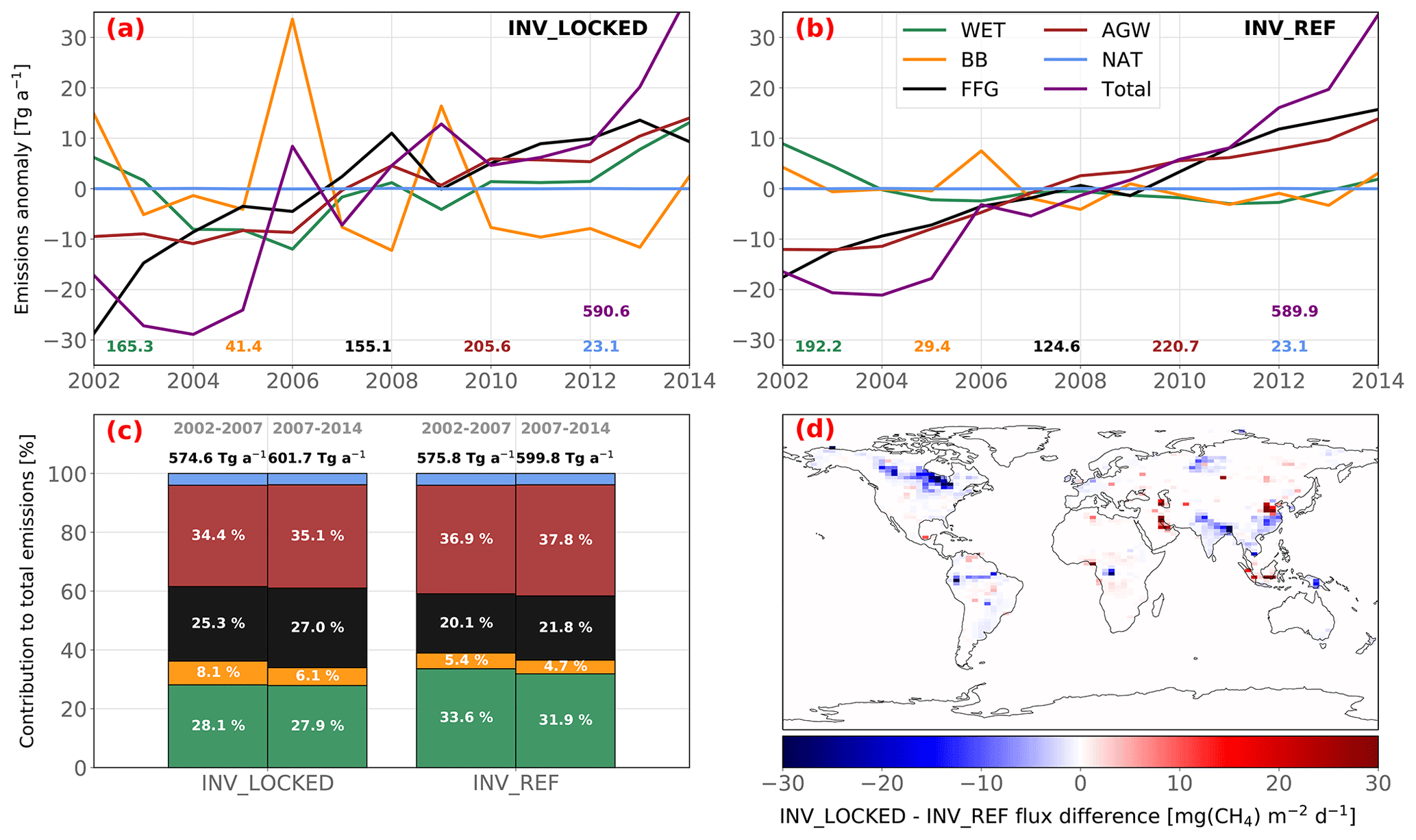
Figure 9Comparison between INV_REF and INV_LOCKED results. Upper panels show the time series of emissions estimated by INV_REF (a) and INV_LOCKED (b). For these panels, the time series show the anomalies around the 2002–2014 mean value. For each category in these panels, the associated mean value is displayed in the same color as the solid line. Lower panels show the contributions from each emission category to the total emissions for 2002–2007 and 2007–2014 (c) and a map of the posterior total emission differences between INV_LOCKED and INV_REF averaged over the 2002–2014 period (d).
3.8 Sensitivity of the results to OH IAV
Last but not least, we have tested the impacts of OH trends on our results. INV_FLATOH and INV_REF show very similar results (Table 5). The main difference is that INV_FLATOH infers a smaller increase in total emissions (+18 Tg a−1) between 2002–2007 and 2007–2014 than INV_REF does (+24 Tg a−1). As a smaller sink is prescribed in INV_FLATOH compared to INV_REF, the increase in total emissions required to fit the observations of CH4 amount fractions is also smaller. The contributions from the emission categories to the total emissions are barely affected (± 0.2 %). The contributions from AGW and FFG emissions to the increase in the total emissions between the two periods are exactly the same as in INV_REF. In addition, as the inter-hemispheric OH ratio is not modified, the contributions from the tropics, mid-latitudes and high latitudes are identical for each emission category. Overall, the differences between INV_REF and INV_FLAT are negligible and do not affect the conclusions deduced from the INV_REF results.
On the contrary, INV_TURNER infers a decline of 1.6 % in global emissions between 2002–2007 and 2007–2014 (Table 5), mainly driven by a large decrease in WET emissions (−15 Tg a−1) and a slightly larger decrease in BB emissions (−4 Tg a−1) than in INV_REF. With this prescribed OH IAV, the renewed CH4 growth post-2007 is therefore entirely caused by a large decline in the global OH sink between the two periods. Changes in AGW and FFG emissions in INV_TURNER are still positive but are 2–3 times smaller than in INV_REF. Using all the information provided by the sensitivity tests inferring a net increase in emissions (i.e., without INV_TURNER), this increase is principally attributed to fossil sources (50 ± 3 %) and agriculture and waste sources (47 ± 5 %). Nevertheless, there is substantial variation in the results between configurations that optimize source signatures and those that do not.
The decline in the OH sink between the two periods affects the δ(13C,CH4) atmospheric signal in two opposite ways:
-
If the OH sink is the only sink, a decline in OH concentrations has no effect on δ(13C,CH4) in the long term (several decades) because the mean fractionation is not affected. However, in the short term (a decade), as OH concentrations decrease, 12CH4 and 13CH4 atmospheric lifetimes increase. Due to the fractionation effect, there is a time lag between increases in 12CH4 and 13CH4 amount fractions. 12CH4 accumulates faster than 13CH4, leading to a decrease in δ(13C,CH4).
-
The total fractionation effect in the atmosphere is the result of averaging all of the fractionation effects associated with the different sinks (OH, O1D, Cl, soils) weighted by their contributions to the total sink. Therefore, if the OH sink is reduced, the contributions from the other sinks (with larger fractionation effects) increase. Consequently, the total fractionation effect is also increased and δ(13C,CH4) values are shifted upward.
As INV_TURNER infers a more depleted global source signature (−0.50 ‰) than INV_REF (−0.34 ‰), we can conclude that the downward shift in δ(13C,CH4) induced by the first mechanism is smaller than the upward shift induced by the second mechanism, resulting in a net upward shift. The enhanced depletion of the global source signature counterbalances this net upward shift. In the inversion, such a depletion is mainly obtained by lowering the source signatures of AGW, FFG and WET sources between 2002–2007 and 2007–2014. Compared to INV_REF, the shifts in source signatures are almost identical for AGW but much larger for FFG and WET. The negative OH trend was obtained by Rigby et al. (2017) and Turner et al. (2017) with box modeling and methyl-chloroform constraints (Patra et al., 2021). However, Naus et al. (2019) suggested that inter-hemispheric transport, stratospheric loss and source and sink spatial distributions are not properly represented using box modeling, resulting in significant errors. They found a positive OH trend over the 1994–2015 period with a 3-D model, which is more consistent with the IAV of our OH-INCA field. Other studies agree with Naus et al. (2019) in finding a small or positive IAV for recent years (Montzka et al., 2011; Lelieveld et al., 2016; Nicely et al., 2018). Therefore, the results from the INV_TURNER inversion seem to be rather unlikely.
3.9 Comparison with Basu et al. (2022)
Basu et al. (2022) – referred to as “BA22” in this subsection – quantify the global CH4 budget and investigate the post-2007 renewed growth, using the TM5-4DVAR inversion framework to assimilate both CH4 and δ(13C,CH4) measurements. In our opinion, their work is strongly relevant and tackles this complex topic with an appropriate and robust methodology. As our goals are similar, we compare our systems and methodologies here.
First, it is worth mentioning that our system is capable of assimilating δ(D,CH4)) observational data and optimizing the associated source signatures. Although this feature has a small influence on our results in this work, we believe that its relevance will grow as more δ(D,CH4)) data become available and the associated uncertainties decrease.
As already stated in their paper, the main difference between our systems is the optimization of source signatures. BA22 prefer to investigate the influence of the source signature uncertainties with different sensitivity tests that adopt various source signature maps. This choice relies on the fact that they can run a large number of inversions at low cost using a parallel configuration. It is a good strategy to assess the influence of systematic errors in source signatures. In our work, we did not investigate this influence, and we decided to optimize source signatures in order to consistently account for random errors in source signatures and emissions at the same time. As both interact and impact the atmospheric composition in very complex ways, it seemed important to us to perform at least one inversion combining all the uncertainties.
We agree with BA22 that the second major difference between the two studies lies in the construction of the prior CH4 fluxes. However, they suggest that we constructed a prior that approximately matches the atmospheric CH4 growth rate in Thanwerdas et al. (2022a). In Thanwerdas et al. (2022a) and in the present study, we derived our prior fluxes and source signatures solely on the basis of bottom-up estimates and literature data. For CH4 emissions, the fact that prior simulations match the atmospheric CH4 growth rate shows that bottom-up estimates are roughly consistent with atmospheric data, even before the inversion process.
We prefer not to adjust prior fluxes to match observational δ(13C,CH4) data because, in this case, we assume that bottom-up estimates suffer from strong systematic uncertainties, which is difficult to demonstrate. When adjusting prior CH4 fluxes, it is also assumed that CH4 emissions derived by bottom-up estimates are more likely to be wrong than source signatures estimates. We believe that the opposite is more plausible because observational data on source signatures are very scarce at present. Therefore, we prefer to start from robust and validated data and let the inversion system combine them with the assimilated atmospheric observations and the random uncertainties. BA22 start with a flat prior, and the posterior results deviate significantly from the prior. As the prior data do not seem to have a strong influence on the posterior results, adjusting prior fluxes prior to the inversion should have no effect on the results. However, this is yet to be confirmed in our case, i.e., with a nonlinear observation operator.
BA22 are able to calculate posterior uncertainties using a large ensemble of inversions. It is a precious feature that we do not possess at present. This is made possible by the relatively low computational cost of their configuration (an adjusted prior and a linear formulation) but also by the fact that they divide the full assimilation window into shorter sub-windows (5 years) that are run in parallel. A 1-year overlap with previous and next sub-windows is applied. It would be interesting to compare the posterior results obtained with this parallelized configuration to an inversion with a complete assimilation window. As the relaxation time for isotopic composition in the atmosphere in response to a perturbation is much larger (decades; Tans, 1997) than that for CH4 itself, we are concerned that using such short time periods might affect posterior results, especially if the observation operator is nonlinear. Modifying the prior data to fit the observed isotopic composition, as in BA22, might be a prerequisite for the success of this method.
It is clear that these setup differences propagate to posterior results. Using the additional δ(13C,CH4) data, BA22 find that fossil CH4 emissions and microbial emissions contributed about 15 % and 85 %, respectively, of the post-2007 CH4 growth. As presented in the previous sections, our results are completely different. Most notably, they find a contribution of 30 % from fossil emissions to the total emissions on average over 1999–2016. While our reference inversion finds a much smaller number (21 %), our inversion with fixed source signatures (INV_LOCKED) gives a closer value (26 %). The small source partitioning discrepancy between INV_LOCKED and BA22's inversion results might also be caused by a difference in prescribed isotopic fractionation, as suggested by the sensitivity analysis of Lan et al. (2021).
We cannot fully explain why BA22's conclusions about the causes of the renewed CH4 growth post-2007 differ so substantially from our own. However, it appears that BA22 also use a robust methodology to study the global CH4 budget and the renewed growth. Despite significant differences, we find good complementarity between our approaches and hope to learn from each other in order to improve our systems and reconcile our results.
We used variational inversion modeling with the 3-D CTM LMDz-SACS to investigate the drivers of the post-2007 renewed growth of atmospheric CH4. We assimilated CH4, δ(13C,CH4) and δ(D,CH4) atmospheric observations and optimized both the fluxes and the source isotopic signatures of five independent emission categories for the period 1998–2017. Implementing multiple setups allowed us to investigate the influences of isotopic constraints and OH IAV on our results.
Most of our inversions find that the post-2007 renewed growth was caused by large increases in fossil fuel and geological emissions (FFG) as well as in agricultural and waste (AGW) emissions between 2002–2007 and 2007–2014. The contributions from these two categories were almost equal (51 % for FFG and 49 % for AGW). These were partially balanced by small decreases in wetland (WET) emissions and biofuel- and biomass-burning (BB) emissions and a small OH increase during this period.
Isotopic constraints, i.e., those achieved by assimilating δ(13C,CH4) and δ(D,CH4) observations, have little influence on the posterior emission estimates. Compared to a CH4-only inversion, an inversion assimilating δ(13C,CH4) observations and optimizing source signatures only slightly reduces tropical emissions (−2.5 Tg a−1), mainly those from wetlands. Notably, the global flux-weighted WET source signature is shifted upward (less negative) due to a shift in the tropics (+3.2 ‰) and in the northern mid-latitudes (+7.1 ‰). To fit the δ(13C,CH4) observations, the system prefers to adjust the source signatures rather than the CH4 emissions. Undoubtedly, the large uncertainties associated with source signatures make them less costly to modify. Our findings also reveal that the global downward shift in δ(13C,CH4) between 2002–2004 and 2007–2014 was caused by an increase in 13C-depleted AGW emissions and a decrease in 13C-enriched BB emissions but also by decreases in the AGW and FFG source signatures. For example, a small change compared to the uncertainties in the AGW source signatures (−0.6 ‰) between the two periods results in a −0.24 ‰ (downward) shift of the global source signature in the reference inversion. These results might be very dependent on the prescribed Cl concentrations, especially in the troposphere, and we decided to use the most recent and consistent Cl concentration estimates to minimize the associated error.
If the δsource(13C,CH4) source signatures are considered to be perfectly known, i.e., with no uncertainty, the relative contributions of the different emission categories are significantly changed by the inversion. Contributions from FFG and BB emissions are increased and those from AGW and WET emissions are decreased. In addition, WET emissions are found to contribute (13 %) to the post-2007 renewed growth, along with AGW (37 %) and FFG (46 %) emissions. Such a partition between fossil and microbial sources is more consistent with recent inversion estimates based on isotopic data. However, none of these recent results account for random uncertainties in source signatures. This shows that reducing the prescribed uncertainties in source signatures is a necessary condition for providing more accurate emission estimates when assimilating isotopic data.
OH IAV also has an influence on the results when a negative trend consistent with the IAV inferred by Turner et al. (2017) is applied. In this case, the post-2007 renewed growth is entirely caused by the decline in OH concentrations, and AGW and FFG emissions only slightly increase over the 2002–2014 period. As recent findings suggest that such a decrease in OH concentrations is unlikely, the results from the other sensitivity inversions should be preferentially considered. Overall, using all the information provided by the sensitivity tests presented in this work, the net increase in global emissions is principally attributed to fossil sources (50 ± 3 %) and agriculture and waste sources (47 ± 5 %).
As this new inversion setup (with isotopic constraints) was used over a long time period for the first time, methods were deliberately simplified in order to provide a background for future inversions and improvements. For instance, our methods to prescribe error statistics in the matrix B obviously have room for improvement, even with the limited amount of data available at the present time. The uncertainties we prescribed for source signatures in the reference inversion might be slightly overestimated. A more robust estimate of current regional random uncertainties in source signatures is necessary before running other inversions with isotopic data.
Also, the main limitation of our inversion system is the associated computational cost and the absence of posterior uncertainties. Formally, posterior uncertainties are given by the Hessian of the cost function (Meirink et al., 2008). This matrix is difficult to compute at an achievable cost considering the size of the inverse problem. Other means must be implemented to obtain the posterior uncertainty, such as estimating a lower-rank approximation of the Hessian using Monte Carlo ensembles of the variational inversion to represent the prior uncertainties (Chevallier, 2007). However, the amount of time required to run a single inversion is too large at present, preventing the derivation of robust posterior statistics as well as attempts to account for systematic uncertainties. Recent developments in the CIF (Chevallier et al., 2023; Chevallier, 2013) may help us to significantly reduce our computational costs and run Monte Carlo ensembles. While these new features have not been tested with realistic configurations yet, preliminary results are promising.
The inversion system proposed in this work benefits from the advantages of both 3-D modeling and variational inversion methods, and it also includes the optimization of the source isotopic signatures. Additionally, it accounts for the observation operator nonlinearity, which is an important component of isotopic data assimilation, particularly when source signatures are also optimized. To our knowledge, such a system is unique and allows us to reconcile emissions and source signatures with the limitation of still-large random uncertainties in the isotopic signatures. More developments are necessary to improve the robustness of the estimates and the relevance of such a system, but we believe that this study represents a significant step towards better quantification of the CH4 sectorial and regional emissions and the global CH4 budget.
Table A1List of surface in situ CH4 observation sites that provided measurements assimilated in the inversions between 1998 and 2018. AOC, PAO, POC and WPC are mobile stations. Their characteristics are compiled into a single line that provides latitude and longitude ranges of the measurements. Stations that retrieved samples consisting mainly of well-mixed marine boundary layer (MBL) air are indicated in bold.
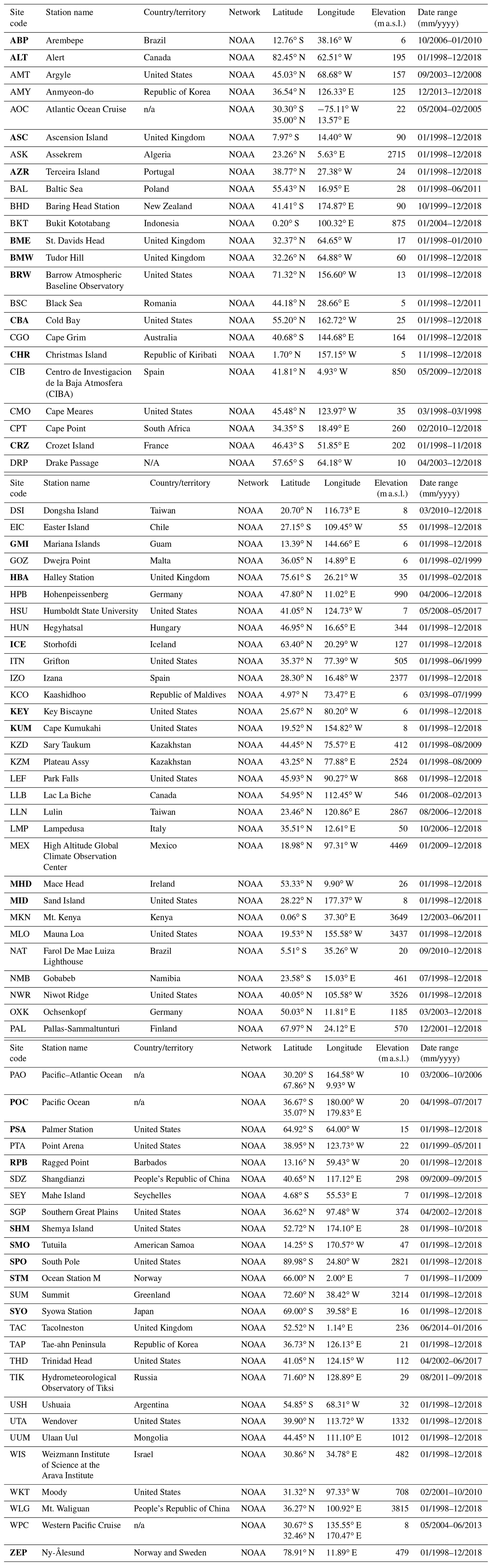
Table A2List of surface in situ δ(13C,CH4) observation sites that provided measurements assimilated in the inversions between 1998 and 2018. WPC is a mobile station. Its characteristics are compiled into a single line that provides latitude and longitude ranges of the measurements. Stations that retrieved samples consisting mainly of well-mixed MBL air are indicated in bold.
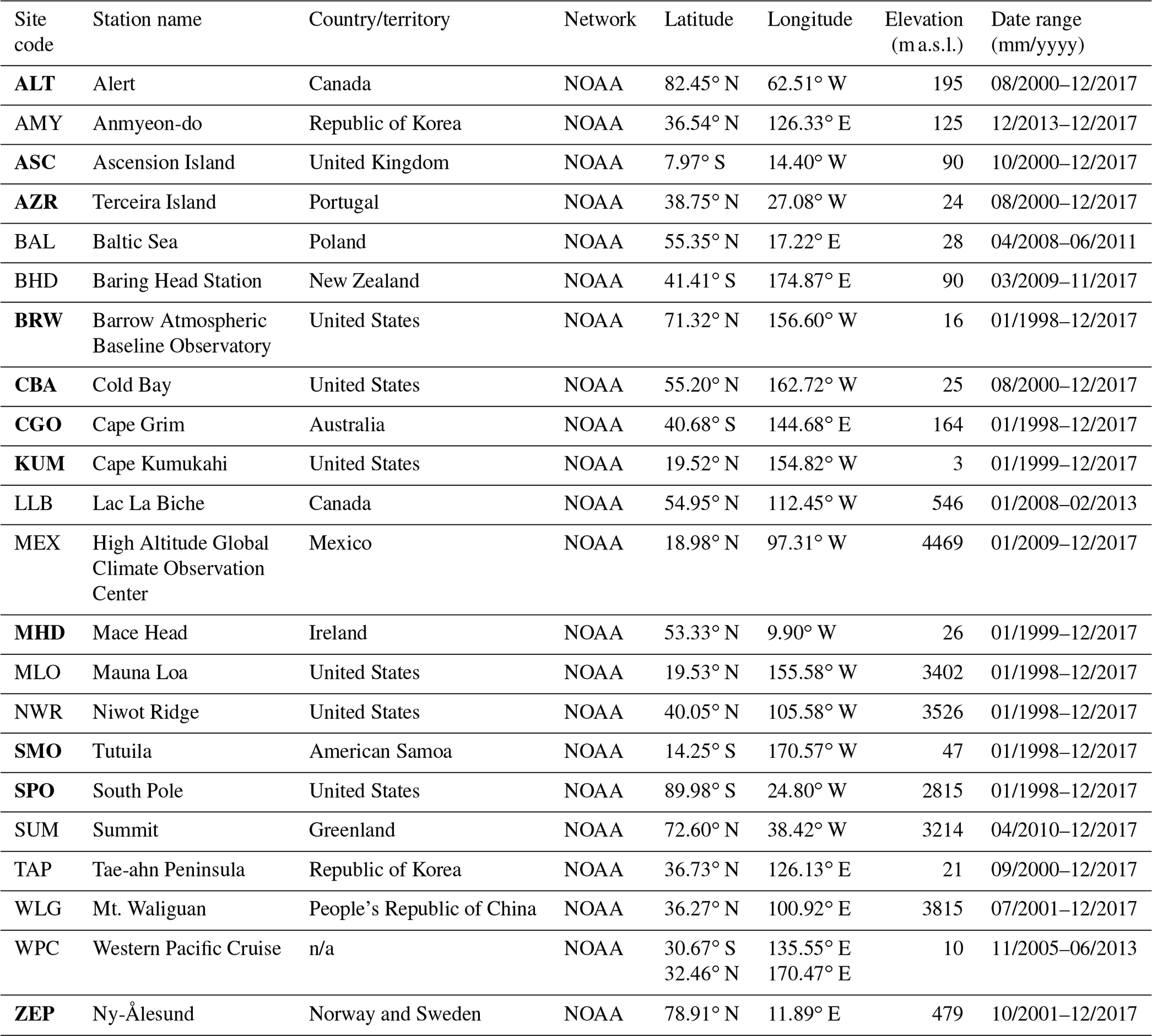
n/a: not applicable.
Table A3List of surface in situ δ(D,CH4) observation sites that provided measurements assimilated in the inversion INV_DD between 2005 and 2010. Stations that retrieved samples consisting mainly of well-mixed MBL air are indicated in bold.
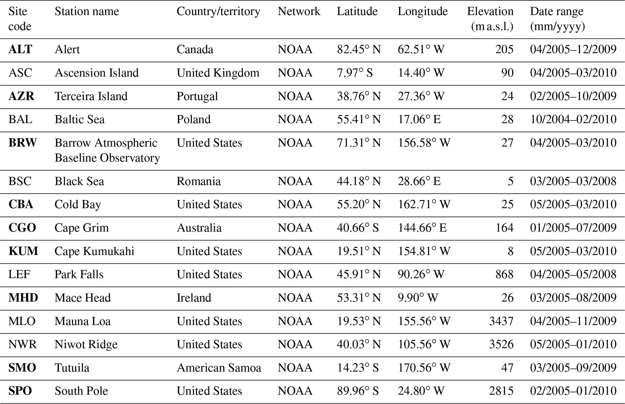
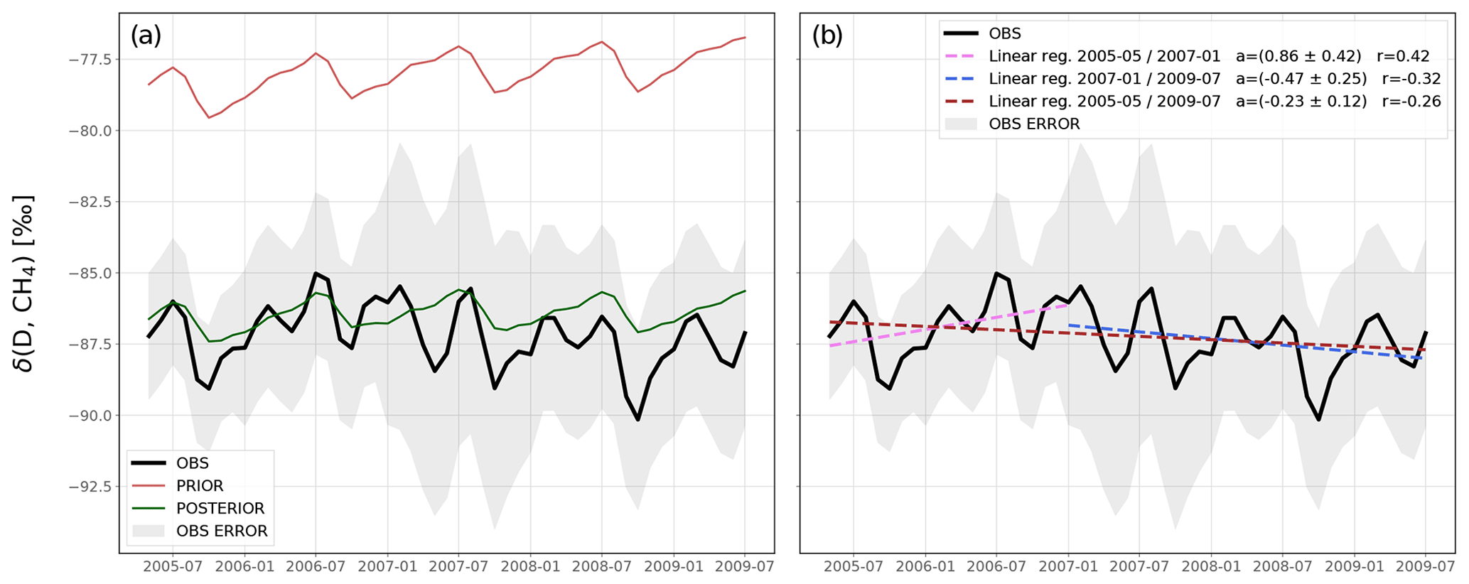
Figure B1Panel (a) shows a comparison between δ(D,CH4) observations and prior and posterior simulations. Panel (b) shows linear regressions applied on the monthly and globally averaged δ(D,CH4) observations. We performed three linear regressions: (1) one over the full data period from May 2005 to July 2009 (brown line), (2) one over the period from May 2005 to January 2007 (violet line), and one over the period from January 2007 to July 2009 (blue line). For each linear regression, the coefficient (a), its standard error and the Pearson's correlation coefficient (r) are displayed in the legend. Note that the x axis stops before 2010, as we have only selected months with sufficient data for the average to be representative of the whole globe.
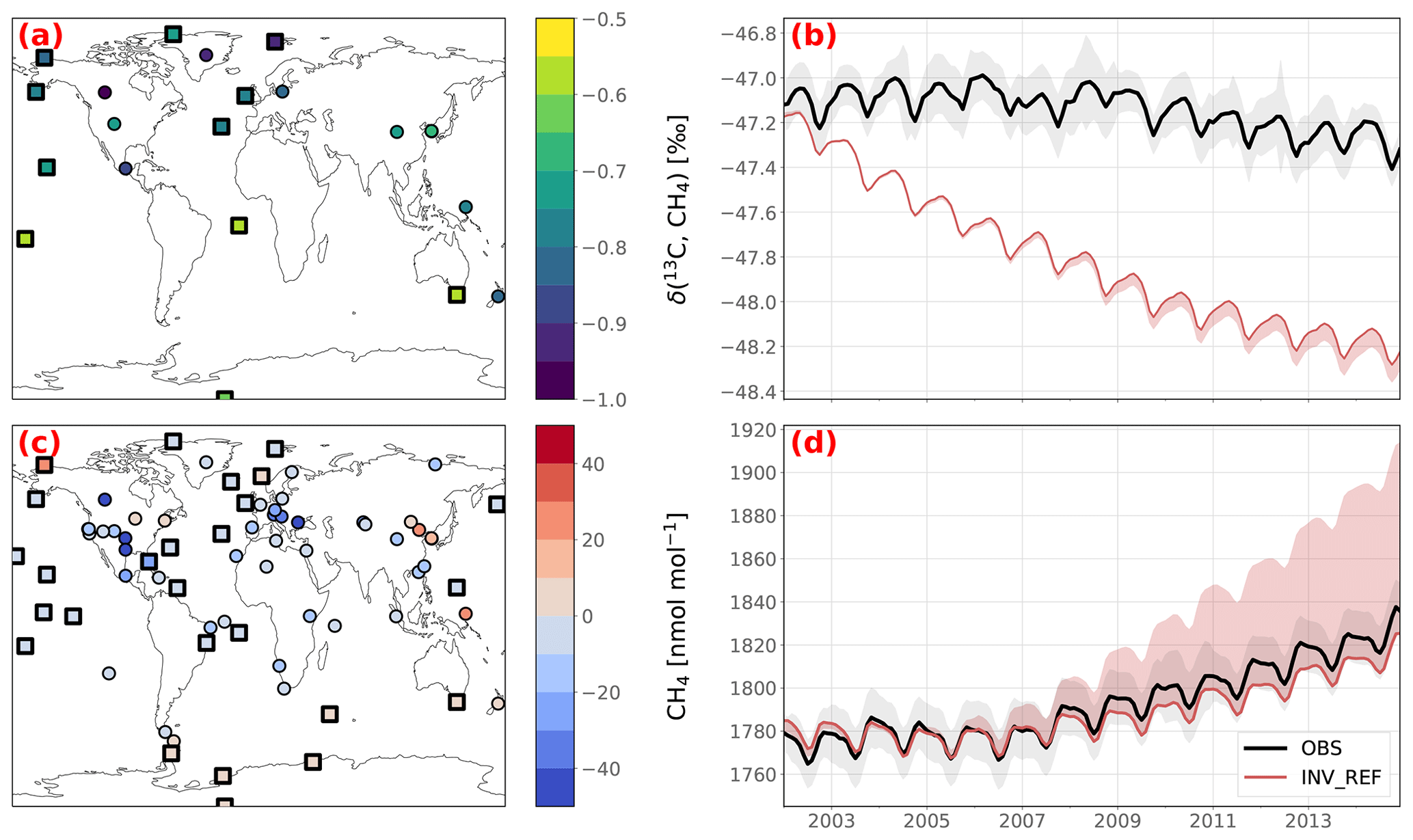
Figure B2Same as Fig. 4 but with prior data. Note that the scale for panel (c) has been modified and is not centered on zero anymore because the prior agreement with δ(13C,CH4) data is too low. The large red-shaded area in panel (d) is caused by a change in the OH sink (INV_TURNER).

Figure B3Comparison between prior–posterior and observed wetland δsource(13C,CH4). Observations are taken from Supplementary Data 1 provided by Oh et al. (2022). For each observation, prior and posterior values are sampled using the grid cell corresponding to the latitude and longitude provided in the dataset. Error bars for each observation point represent the observation uncertainty. Each panel shows a comparison with observations located in a selected region: the tropics (<30∘ N/S), temperate (30–50∘ N/S), western boreal (50–90∘ N and <15∘ W) and eastern boreal (50–90∘ N and >15∘ W). For each panel, the identity line and two linear fitting lines (prior in green and posterior in red) are displayed. The parameters of the fitting lines, the Pearson's correlation coefficients (r) and the root-mean-square error (RMSE) are given in the legend box.
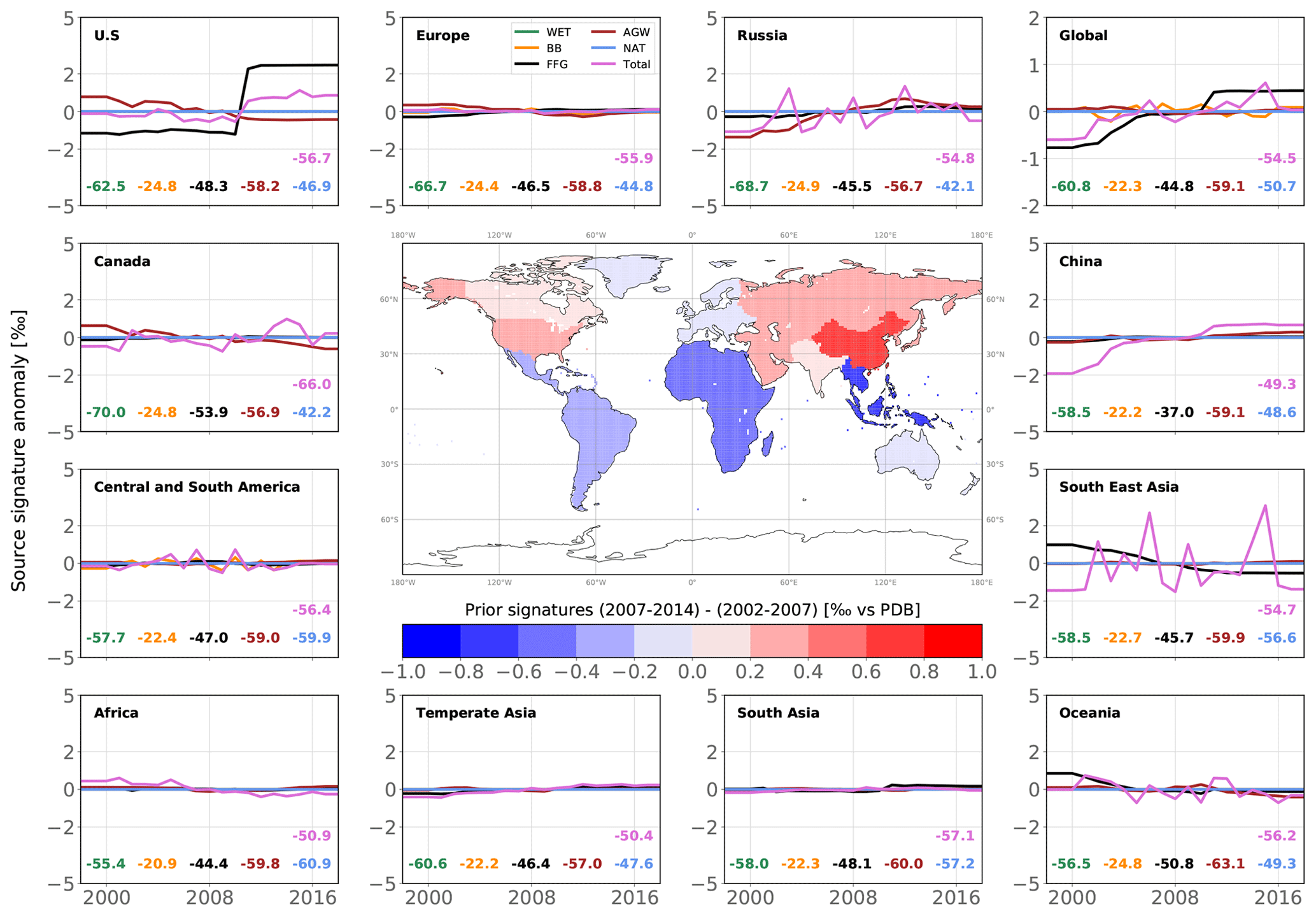
Figure B4Same as Fig.7 but for prior source signatures δsource(13C,CH4). For each panel, the time series show the anomalies around the 2002–2014 mean value. The units of variations and means are ‰. Note that x axis ranges from 1998–2018 to illustrate the effects of the spin-up and spin-down mentioned in Sect. 2.8. Also note that the regions used here are slightly different from the regions selected for the optimization.
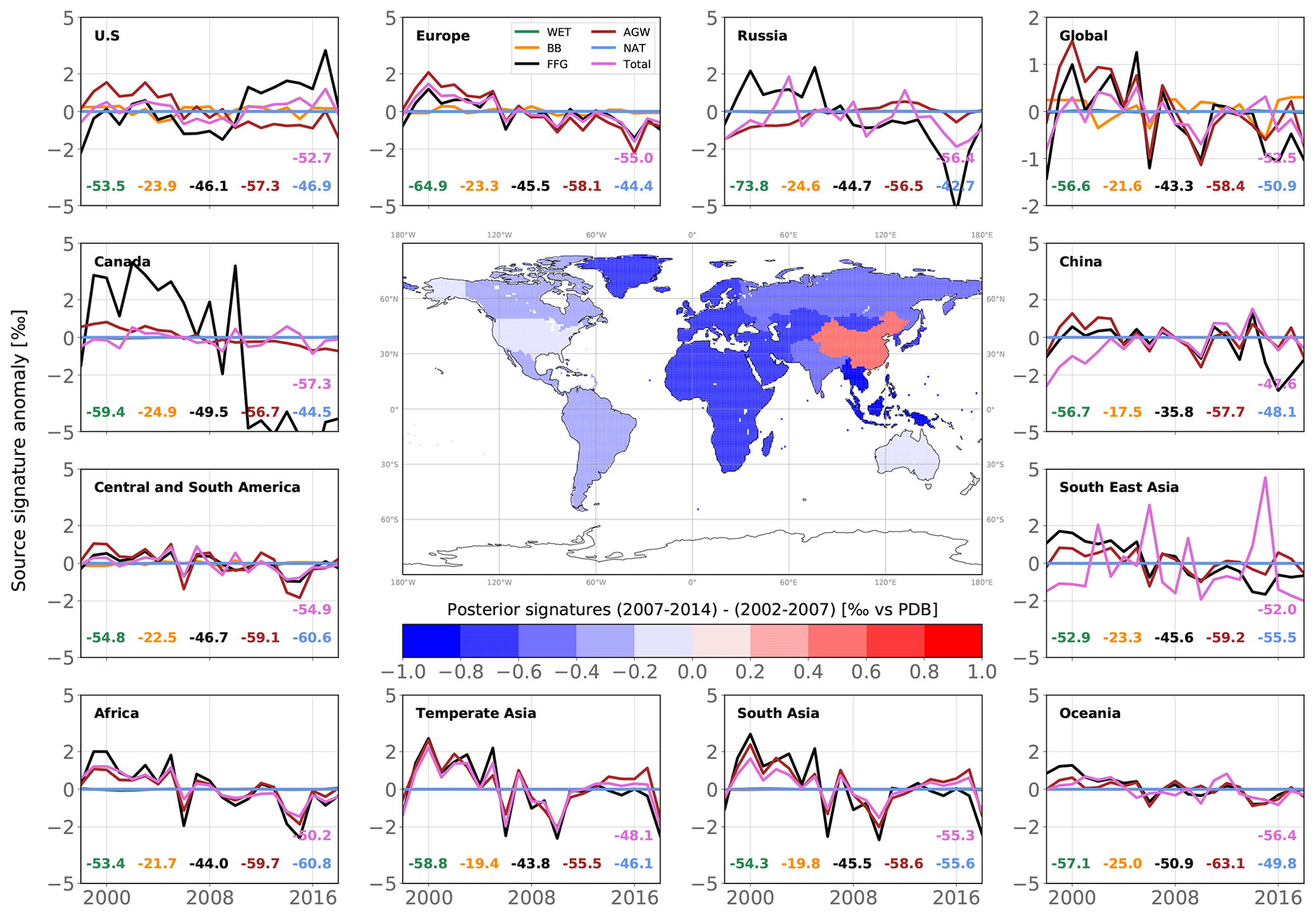
Figure B5Same as Fig. B4 but for posterior source signatures δsource(13C,CH4) from INV_REF. Note that the green (WET) and blue (NAT) lines are flat because (1) the prior signatures are constant over time, (2) these categories do not result from the aggregation of multiple subcategories and (3) we optimize only one scaling factor per region for the entire period. Therefore, these values do not vary with time. Also, note that BB source signatures vary only because the regions used here are slightly different from the regions selected for the optimization. Therefore, the flux-weighted average produces some temporal variability.
Table B1Posterior CH4 emissions for the globe and three different latitudinal bands averaged over 2002–2014 for all inversions and all categories. The units of the values shown are Tg a−1.
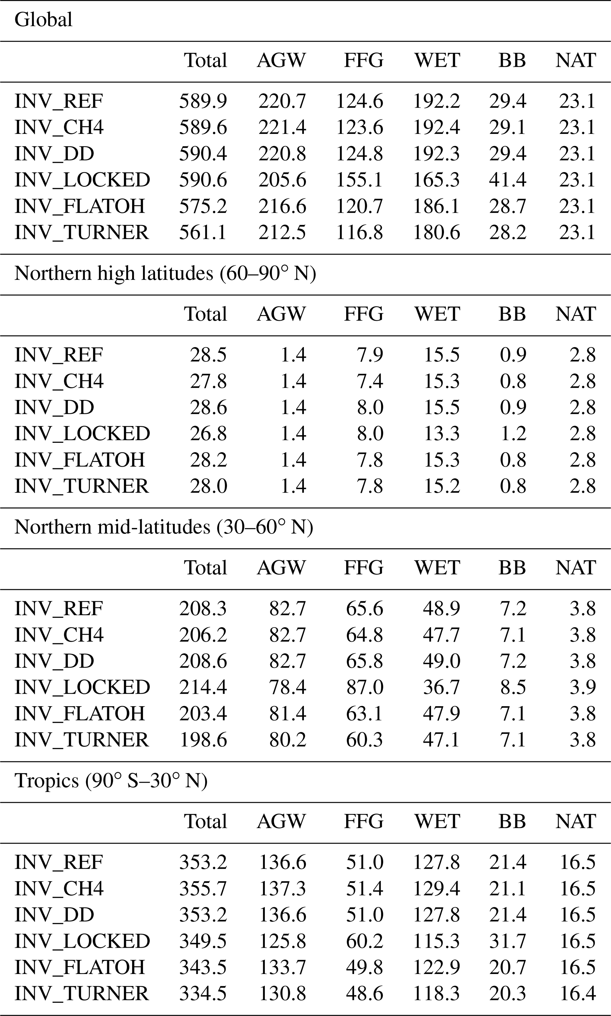
The code files of the CIF version used in the present paper are registered under the following DOI: https://doi.org/10.5281/zenodo.6304912 (Berchet et al., 2022). The CH4 (Lan et al., 2022), δ(13C,CH4) (White et al., 2021) and δ(D,CH4) (White et al., 2016) observational data can be downloaded directly from the NOAA-GML website (https://esrl.noaa.gov/gmd/aftp/data/trace_gases, last access: 12 July 2021). All the other relevant data used to perform the inversions are registered under the following DOI: https://doi.org/10.5281/zenodo.10390430 (Thanwerdas, 2023).
JT designed and ran the inversions and performed the data analysis presented in this paper. MS, AB, IP and PB provided scientific and technical expertise and contributed to the scientific analysis of this work. JT prepared the paper, with contributions from all co-authors.
The contact author has declared that none of the authors has any competing interests.
Publisher’s note: Copernicus Publications remains neutral with regard to jurisdictional claims made in the text, published maps, institutional affiliations, or any other geographical representation in this paper. While Copernicus Publications makes every effort to include appropriate place names, the final responsibility lies with the authors.
The study extensively relies on the meteorological data provided by the ECMWF. Calculations were performed using the computing resources of LSCE, which are maintained by Julien Bruna, François Marabelle and the rest of the LSCE IT team. The authors wish to thank the measurement teams from the NOAA GML and from INSTAAR for their continuous and high-quality work. In particular, the authors would like to express their special thanks to Xin Lan from NOAA and to Sylvia E. Michel, Bruce H. Vaughn and Reid Clark from INSTAAR for their invaluable help and helpful comments, which greatly improved the quality of the submitted draft. Finally, the authors are grateful to the two anonymous referees and the editor for their invaluable insights, which greatly enhanced the quality of the paper.
This research has been supported by the Commissariat à l'Énergie Atomique et aux Énergies Alternatives (grant no. CFR 2018).
This paper was edited by Jan Kaiser and reviewed by two anonymous referees.
Allan, W., Struthers, H., and Lowe, D. C.: Methane carbon isotope effects caused by atomic chlorine in the marine boundary layer: Global model results compared with Southern Hemisphere measurements, J. Geophys. Res., 112, D04306, https://doi.org/10.1029/2006JD007369, 2007. a
Bader, W., Bovy, B., Conway, S., Strong, K., Smale, D., Turner, A. J., Blumenstock, T., Boone, C., Collaud Coen, M., Coulon, A., Garcia, O., Griffith, D. W. T., Hase, F., Hausmann, P., Jones, N., Krummel, P., Murata, I., Morino, I., Nakajima, H., O'Doherty, S., Paton-Walsh, C., Robinson, J., Sandrin, R., Schneider, M., Servais, C., Sussmann, R., and Mahieu, E.: The recent increase of atmospheric methane from 10 years of ground-based NDACC FTIR observations since 2005, Atmos. Chem. Phys., 17, 2255–2277, https://doi.org/10.5194/acp-17-2255-2017, 2017. a, b, c
Basu, S., Lan, X., Dlugokencky, E., Michel, S., Schwietzke, S., Miller, J. B., Bruhwiler, L., Oh, Y., Tans, P. P., Apadula, F., Gatti, L. V., Jordan, A., Necki, J., Sasakawa, M., Morimoto, S., Di Iorio, T., Lee, H., Arduini, J., and Manca, G.: Estimating emissions of methane consistent with atmospheric measurements of methane and δ13C of methane, Atmos. Chem. Phys., 22, 15351–15377, https://doi.org/10.5194/acp-22-15351-2022, 2022. a, b, c, d, e, f
Berchet, A., Sollum, E., Thompson, R. L., Pison, I., Thanwerdas, J., Broquet, G., Chevallier, F., Aalto, T., Berchet, A., Bergamaschi, P., Brunner, D., Engelen, R., Fortems-Cheiney, A., Gerbig, C., Groot Zwaaftink, C. D., Haussaire, J.-M., Henne, S., Houweling, S., Karstens, U., Kutsch, W. L., Luijkx, I. T., Monteil, G., Palmer, P. I., van Peet, J. C. A., Peters, W., Peylin, P., Potier, E., Rödenbeck, C., Saunois, M., Scholze, M., Tsuruta, A., and Zhao, Y.: The Community Inversion Framework v1.0: a unified system for atmospheric inversion studies, Geosci. Model Dev., 14, 5331–5354, https://doi.org/10.5194/gmd-14-5331-2021, 2021. a
Berchet, A., Sollum, E., Pison, I., Thompson, R. L., Thanwerdas, J., Fortems-Cheiney, A., Peet, J. C. A. v., Potier, E., Chevallier, F., Broquet, G., and Berchet, A.: The Community Inversion Framework: codes and documentation, Zenodo [code], https://doi.org/10.5281/zenodo.6304912, 2022. a
Bergamaschi, P., Lubina, C., Königstedt, R., Fischer, H., Veltkamp, A. C., and Zwaagstra, O.: Stable isotopic signatures (δ13C, δD) of methane from European landfill sites, J. Geophys. Res.-Atmos., 103, 8251–8265, https://doi.org/10.1029/98JD00105, 1998. a
Bousquet, P., Hauglustaine, D. A., Peylin, P., Carouge, C., and Ciais, P.: Two decades of OH variability as inferred by an inversion of atmospheric transport and chemistry of methyl chloroform, Atmos. Chem. Phys., 5, 2635–2656, https://doi.org/10.5194/acp-5-2635-2005, 2005. a
Bousquet, P., Ciais, P., Miller, J. B., Dlugokencky, E. J., Hauglustaine, D. A., Prigent, C., Van der Werf, G. R., Peylin, P., Brunke, E.-G., Carouge, C., Langenfelds, R. L., Lathière, J., Papa, F., Ramonet, M., Schmidt, M., Steele, L. P., Tyler, S. C., and White, J.: Contribution of anthropogenic and natural sources to atmospheric methane variability, Nature, 443, 439–443, https://doi.org/10.1038/nature05132, 2006. a, b, c, d
Bréas, O., Guillou, C., Reniero, F., and Wada, E.: The Global Methane Cycle: Isotopes and Mixing Ratios, Sources and Sinks, Isot. Environ. Healt. S., 37, 257–379, https://doi.org/10.1080/10256010108033302, 2001. a
Burkholder, J. B., Sander, S. P., Abbatt, J., Barker, J. R., Cappa, C., Crounse, J. D., Dibble, T. S., Huie, R. E., Kolb, C. E., Kurylo, M. J., Orkin, V. L., Percival, C. J., Wilmouth, D. M., and Wine, P. H.: Chemical Kinetics and Photochemical Data for Use in Atmospheric Studies, Evaluation No. 19, JPL Publication 19-5, Jet Propulsion Laboratory, Pasadena, 2019 http://jpldataeval.jpl.nasa.gov (last access: 9 February 2024), 2019. a
Cantrell, C. A., Shetter, R. E., McDaniel, A. H., Calvert, J. G., Davidson, J. A., Lowe, D. C., Tyler, S. C., Cicerone, R. J., and Greenberg, J. P.: Carbon kinetic isotope effect in the oxidation of methane by the hydroxyl radical, J. Geophys. Res.-Atmos., 95, 22455–22462, https://doi.org/10.1029/JD095iD13p22455, 1990. a, b, c, d
Chandra, N., Patra, P. K., Bisht, J. S. H., Ito, A., Umezawa, T., Saigusa, N., Morimoto, S., Aoki, S., Janssens-Maenhout, G., Fujita, R., Takigawa, M., Watanabe, S., Saitoh, N., and Canadell, J. G.: Emissions from the Oil and Gas Sectors, Coal Mining and Ruminant Farming Drive Methane Growth over the Past Three Decades, J. Meteorol. Soc. Jpn. Ser. II, 99, 309–337, https://doi.org/10.2151/jmsj.2021-015, 2021. a, b, c, d, e, f, g
Chang, J., Peng, S., Ciais, P., Saunois, M., Dangal, S. R. S., Herrero, M., Havlík, P., Tian, H., and Bousquet, P.: Revisiting enteric methane emissions from domestic ruminants and their δ13C source signature, Nat. Commun., 10, 3420, https://doi.org/10.1038/s41467-019-11066-3, 2019. a, b
Chanton, J. P., Rutkowski, C. M., and Mosher, B.: Quantifying Methane Oxidation from Landfills Using Stable Isotope Analysis of Downwind Plumes, Environ. Sci. Technol., 33, 3755–3760, https://doi.org/10.1021/es9904033, 1999. a
Chanton, J. P., Rutkowski, C. M., Schwartz, C. C., Ward, D. E., and Boring, L.: Factors influencing the stable carbon isotopic signature of methane from combustion and biomass burning, J. Geophys. Res.-Atmos., 105, 1867–1877, https://doi.org/10.1029/1999JD900909, 2000. a
Chevallier, F.: Impact of correlated observation errors on inverted CO2 surface fluxes from OCO measurements, Geophys. Res. Lett., 34, 24, https://doi.org/10.1029/2007GL030463, 2007. a
Chevallier, F.: On the parallelization of atmospheric inversions of CO2 surface fluxes within a variational framework, Geosci. Model Dev., 6, 783–790, https://doi.org/10.5194/gmd-6-783-2013, 2013. a, b
Chevallier, F., Fisher, M., Peylin, P., Serrar, S., Bousquet, P., Bréon, F.-M., Chédin, A., and Ciais, P.: Inferring CO2 sources and sinks from satellite observations: Method and application to TOVS data, J. Geophys. Res., 110, D24, https://doi.org/10.1029/2005JD006390, 2005. a
Chevallier, F., Lloret, Z., Cozic, A., Takache, S., and Remaud, M.: Toward High-Resolution Global Atmospheric Inverse Modeling Using Graphics Accelerators, Geophys. Res. Lett., 50, e2022GL102135, https://doi.org/10.1029/2022GL102135, 2023. a
Craig, H.: Isotopic standards for carbon and oxygen and correction factors for mass-spectrometric analysis of carbon dioxide, Geochim. Cosmochim. Ac., 12, 133–149, https://doi.org/10.1016/0016-7037(57)90024-8, 1957. a
Dalsøren, S. B., Myhre, C. L., Myhre, G., Gomez-Pelaez, A. J., Søvde, O. A., Isaksen, I. S. A., Weiss, R. F., and Harth, C. M.: Atmospheric methane evolution the last 40 years, Atmos. Chem. Phys., 16, 3099–3126, https://doi.org/10.5194/acp-16-3099-2016, 2016. a
Enting, I. G. and Newsam, G. N.: Atmospheric constituent inversion problems: Implications for baseline monitoring, J. Atmos. Chem., 11, 69–87, https://doi.org/10.1007/BF00053668, 1990. a
Etiope, G.: Natural Gas Seepage: The Earth’s Hydrocarbon Degassing, Springer International Publishing, ISBN 978-3-319-14600-3, https://doi.org/10.1007/978-3-319-14601-0_8, 2015. a, b
Etiope, G., Ciotoli, G., Schwietzke, S., and Schoell, M.: Gridded maps of geological methane emissions and their isotopic signature, Earth Syst. Sci. Data, 11, 1–22, https://doi.org/10.5194/essd-11-1-2019, 2019. a
Feinberg, A. I., Coulon, A., Stenke, A., Schwietzke, S., and Peter, T.: Isotopic source signatures: Impact of regional variability on the δ13C(CH4) trend and spatial distribution, Atmos. Environ., 174, 99–111, https://doi.org/10.1016/j.atmosenv.2017.11.037, 2018. a, b, c, d
Forster, P., Storelvmo, T., Armour, K., Collins, W., Dufresne, J. L., Frame, D., Lunt, D. J., Mauritsen, T., Palmer, M. D., Watanabe, M., Wild, M., and Zhang, H.: The Earth’s Energy Budget, Climate Feedbacks, and Climate Sensitivity, in: Climate Change 2021: The Physical Science Basis. Contribution of Working Group I to the Sixth Assessment Report of the Intergovernmental Panel on Climate Change, edited by: Masson-Delmotte, V., Zhai, P., Pirani, A., Connors, S. L., Péan, C., Berger, S., Caud, N., Chen, Y., Goldfarb, L., Gomis, M. I., Huang, M., Leitzell, K., Lonnoy, E., Matthews, J. B. R., Maycock, T. K., Waterfield, T., Yelekçi, O., Yu, R. and Zhou, B., Cambridge University Press, Cambridge, United Kingdom and New York, NY, USA, 923–1054, https://doi.org/10.1017/9781009157896.009, 2021. a
Fujita, R., Morimoto, S., Maksyutov, S., Kim, H.-S., Arshinov, M., Brailsford, G., Aoki, S., and Nakazawa, T.: Global and Regional CH4 Emissions for 1995–2013 Derived From Atmospheric CH4, δ13C-CH4, and δD-CH4 Observations and a Chemical Transport Model, J. Geophys. Res.-Atmos., 125, e2020JD032903, https://doi.org/10.1029/2020JD032903, 2020. a, b
Ganesan, A. L., Stell, A. C., Gedney, N., Comyn-Platt, E., Hayman, G., Rigby, M., Poulter, B., and Hornibrook, E. R. C.: Spatially Resolved Isotopic Source Signatures of Wetland Methane Emissions, Geophys. Res. Lett., 45, 3737–3745, https://doi.org/10.1002/2018GL077536, 2018. a, b, c, d, e
Gilbert, J. C. and Lemaréchal, C.: Some numerical experiments with variable-storage quasi-Newton algorithms, Math. Program., 45, 407–435, https://doi.org/10.1007/BF01589113, 1989. a
Gulev, S. K., Thorne, P. W., Ahn, J., Dentener, F. J., Domingues, C. M., Gerland, S., Gong, D., Kaufman, D. S., Nnamchi, H. C., Quaas, J., Rivera, J. A., Sathyendranath, S., Smith, S. L., Trewin, B., von Shuckmann, K., and Vose, R.: Changing State of the Climate System, in: Climate Change 2021: The Physical Science Basis, Contribution of Working Group I to the Sixth Assessment Report of the Intergovernmental Panel on Climate Change, edited by: Masson-Delmotte, V., Zhai, P., Pirani, A., Connors, S. L., Péan, C., Berger, S., Caud, N., Chen, Y., Goldfarb, L., Gomis, M. I., Huang, M., Leitzell, K., Lonnoy, E., Matthews, J. B. R., Maycock, T. K., Waterfield, T., Yelekçi, O., Yu, R., and Zhou, B., Cambridge University Press, Cambridge, United Kingdom and New York, NY, USA, 287–422, https://doi.org/10.1017/9781009157896.004, 2021. a
Hagemann, R., Nief, G., and Roth, E.: Absolute isotopic scale for deuterium analysis of natural waters, Absolute D H ratio for SMOW1, Tellus, 22, 712–715, https://doi.org/10.1111/j.2153-3490.1970.tb00540.x, 1970. a
Hauglustaine, D. A., Hourdin, F., Jourdain, L., Filiberti, M.-A., Walters, S., Lamarque, J.-F., and Holland, E. A.: Interactive chemistry in the Laboratoire de Météorologie Dynamique general circulation model: Description and background tropospheric chemistry evaluation, J. Geophys. Res.-Atmos., 109, D4, https://doi.org/10.1029/2003JD003957, 2004. a
Hausmann, P., Sussmann, R., and Smale, D.: Contribution of oil and natural gas production to renewed increase in atmospheric methane (2007–2014): top–down estimate from ethane and methane column observations, Atmos. Chem. Phys., 16, 3227–3244, https://doi.org/10.5194/acp-16-3227-2016, 2016. a
He, J., Naik, V., Horowitz, L. W., Dlugokencky, E., and Thoning, K.: Investigation of the global methane budget over 1980-2017 using GFDL-AM4.1, Atmos. Chem. Phys., 20, 805–827, https://doi.org/10.5194/acp-20-805-2020, 2020. a
Holmes, M. E., Sansone, F. J., Rust, T. M., and Popp, B. N.: Methane production, consumption, and air-sea exchange in the open ocean: An Evaluation based on carbon isotopic ratios, Global Biogeochem. Cy., 14, 1–10, https://doi.org/10.1029/1999GB001209, 2000. a
Hossaini, R., Chipperfield, M. P., Saiz-Lopez, A., Fernandez, R., Monks, S., Feng, W., Brauer, P., and von Glasow, R.: A global model of tropospheric chlorine chemistry: Organic versus inorganic sources and impact on methane oxidation, J. Geophys. Res.-Atmos., 121, 14271–14297, https://doi.org/10.1002/2016JD025756, 2016. a
Hourdin, F., Musat, I., Bony, S., Braconnot, P., Codron, F., Dufresne, J.-L., Fairhead, L., Filiberti, M.-A., Friedlingstein, P., Grandpeix, J.-Y., Krinner, G., LeVan, P., Li, Z.-X., and Lott, F.: The LMDZ4 general circulation model: climate performance and sensitivity to parametrized physics with emphasis on tropical convection, Clim. Dynam., 27, 787–813, https://doi.org/10.1007/s00382-006-0158-0, 2006. a
Houweling, S., Bergamaschi, P., Chevallier, F., Heimann, M., Kaminski, T., Krol, M., Michalak, A. M., and Patra, P.: Global inverse modeling of CH4 sources and sinks: an overview of methods, Atmos. Chem. Phys., 17, 235–256, https://doi.org/10.5194/acp-17-235-2017, 2017. a, b
Höglund-Isaksson, L.: Global anthropogenic methane emissions 2005-2030: technical mitigation potentials and costs, Atmos. Chem. Phys., 12, 9079–9096, https://doi.org/10.5194/acp-12-9079-2012, 2012. a
Höglund-Isaksson, L.: Bottom-up simulations of methane and ethane emissions from global oil and gas systems 1980 to 2012, Environ. Res. Lett., 12, 024007, https://doi.org/10.1088/1748-9326/aa583e, 2017. a
Ide, K., Courtier, P., Ghil, M., and Lorenc, A. C.: Unified Notation for Data Assimilation: Operational, Sequential and Variational (gtSpecial IssueltData Assimilation in Meteology and Oceanography: Theory and Practice), J. Meteorol. Soc. Jpn. Ser. II, 75, 181–189, https://doi.org/10.2151/jmsj1965.75.1B_181, 1997. a
Jackson, R. B., Saunois, M., Bousquet, P., Canadell, J. G., Poulter, B., Stavert, A. R., Bergamaschi, P., Niwa, Y., Segers, A., and Tsuruta, A.: Increasing anthropogenic methane emissions arise equally from agricultural and fossil fuel sources, Environ. Res. Lett., 15, 071002, https://doi.org/10.1088/1748-9326/ab9ed2, 2020. a, b, c, d
Janssens-Maenhout, G., Crippa, M., Guizzardi, D., Muntean, M., Schaaf, E., Dentener, F., Bergamaschi, P., Pagliari, V., Olivier, J. G. J., Peters, J. A. H. W., van Aardenne, J. A., Monni, S., Doering, U., Petrescu, A. M. R., Solazzo, E., and Oreggioni, G. D.: EDGAR v4.3.2 Global Atlas of the three major greenhouse gas emissions for the period 1970–2012, Earth Syst. Sci. Data, 11, 959–1002, https://doi.org/10.5194/essd-11-959-2019, 2019. a, b
King, S. L., Quay, P. D., and Lansdown, J. M.: The 13C 12C kinetic isotope effect for soil oxidation of methane at ambient atmospheric concentrations, J. Geophys. Res.-Atmos., 94, 18273–18277, https://doi.org/10.1029/JD094iD15p18273, 1989. a
Kirschke, S., Bousquet, P., Ciais, P., Saunois, M., Canadell, J. G., Dlugokencky, E. J., Bergamaschi, P., Bergmann, D., Blake, D. R., Bruhwiler, L., Cameron-Smith, P., Castaldi, S., Chevallier, F., Feng, L., Fraser, A., Heimann, M., Hodson, E. L., Houweling, S., Josse, B., Fraser, P. J., Krummel, P. B., Lamarque, J.-F., Langenfelds, R. L., Le Quéré, C., Naik, V., O'Doherty, S., Palmer, P. I., Pison, I., Plummer, D., Poulter, B., Prinn, R. G., Rigby, M., Ringeval, B., Santini, M., Schmidt, M., Shindell, D. T., Simpson, I. J., Spahni, R., Steele, L. P., Strode, S. A., Sudo, K., Szopa, S., van der Werf, G. R., Voulgarakis, A., van Weele, M., Weiss, R. F., Williams, J. E., and Zeng, G.: Three decades of global methane sources and sinks, Nat. Geosci., 6, 813–823, https://doi.org/10.1038/ngeo1955, 2013. a
Klevenhusen, F., Bernasconi, S. M., Kreuzer, M., and Soliva, C. R.: Experimental validation of the Intergovernmental Panel on Climate Change default values for ruminant-derived methane and its carbon-isotope signature, Anim. Prod. Sci., 50, 159–167, https://doi.org/10.1071/AN09112, 2010. a
Kuze, A., Suto, H., Shiomi, K., Kawakami, S., Tanaka, M., Ueda, Y., Deguchi, A., Yoshida, J., Yamamoto, Y., Kataoka, F., Taylor, T. E., and Buijs, H. L.: Update on GOSAT TANSO-FTS performance, operations, and data products after more than 6 years in space, Atmos. Meas. Tech., 9, 2445–2461, https://doi.org/10.5194/amt-9-2445-2016, 2016. a
Lambert, G. and Schmidt, S.: Reevaluation of the oceanic flux of methane: Uncertainties and long term variations, Chemosphere, 26, 579–589, https://doi.org/10.1016/0045-6535(93)90443-9, 1993. a
Lan, X., Basu, S., Schwietzke, S., Bruhwiler, L. M. P., Dlugokencky, E. J., Michel, S. E., Sherwood, O. A., Tans, P. P., Thoning, K., Etiope, G., Zhuang, Q., Liu, L., Oh, Y., Miller, J. B., Pétron, G., Vaughn, B. H., and Crippa, M.: Improved Constraints on Global Methane Emissions and Sinks Using δ13C-CH4, Global Biogeochem. Cy., 35, e2021GB007000, https://doi.org/10.1029/2021GB007000, 2021. a, b, c
Lan, X., Dlugokencky, E. J., Mund, J., Crotwell, A., Crotwell, M., Moglia, E., Madronich, M., Neff, D., and Thoning, K.: Atmospheric Methane Dry Air Mole Fractions from the NOAA GML Carbon Cycle Cooperative Global Air Sampling Network, 1983–2021, Version: 2022-11-21, NOAA [data set], https://doi.org/10.15138/VNCZ-M766, 2022. a, b
Lan, X., Thoning, K., and Dlugokencky, E. J.: Trends in globally-averaged CH4, N2O, and SF6 determined from NOAA Global Monitoring Laboratory measurements, Version 2023-02, https://doi.org/10.15138/P8XG-AA10, 2023. a
Langenfelds, R. L., Francey, R. J., Pak, B. C., Steele, L. P., Lloyd, J., Trudinger, C. M., and Allison, C. E.: Interannual growth rate variations of atmospheric CO2 and its δ13C, H2, CH4, and CO between 1992 and 1999 linked to biomass burning, Global Biogeochem. Cy., 16, 21-1–21-22, https://doi.org/10.1029/2001GB001466, 2002. a
Lelieveld, J., Gromov, S., Pozzer, A., and Taraborrelli, D.: Global tropospheric hydroxyl distribution, budget and reactivity, Atmos. Chem. Phys., 16, 12477–12493, https://doi.org/10.5194/acp-16-12477-2016, 2016. a
Levin, I., Bergamaschi, P., Dörr, H., and Trapp, D.: Stable isotopic signature of methane from major sources in Germany, Chemosphere, 26, 161–177, https://doi.org/10.1016/0045-6535(93)90419-6, 1993. a
Locatelli, R., Bousquet, P., Saunois, M., Chevallier, F., and Cressot, C.: Sensitivity of the recent methane budget to LMDz sub-grid-scale physical parameterizations, Atmos. Chem. Phys., 15, 9765–9780, https://doi.org/10.5194/acp-15-9765-2015, 2015. a
Louis, J.-F.: A parametric model of vertical eddy fluxes in the atmosphere, Bound.-Lay. Meteorol., 17, 187–202, https://doi.org/10.1007/BF00117978, 1979. a
Lu, X., Jacob, D. J., Zhang, Y., Maasakkers, J. D., Sulprizio, M. P., Shen, L., Qu, Z., Scarpelli, T. R., Nesser, H., Yantosca, R. M., Sheng, J., Andrews, A., Parker, R. J., Boesch, H., Bloom, A. A., and Ma, S.: Global methane budget and trend, 2010–2017: complementarity of inverse analyses using in situ (GLOBALVIEWplus CH4 ObsPack) and satellite (GOSAT) observations, Atmos. Chem. Phys., 21, 4637–4657, https://doi.org/10.5194/acp-21-4637-2021, 2021. a
Masarie, K. A. and Tans, P. P.: Extension and integration of atmospheric carbon dioxide data into a globally consistent measurement record, J. Geophys. Res.-Atmos., 100, 11593–11610, https://doi.org/10.1029/95JD00859, 1995. a
McNorton, J., Wilson, C., Gloor, M., Parker, R. J., Boesch, H., Feng, W., Hossaini, R., and Chipperfield, M. P.: Attribution of recent increases in atmospheric methane through 3-D inverse modelling, Atmos. Chem. Phys., 18, 18149–18168, https://doi.org/10.5194/acp-18-18149-2018, 2018. a, b, c, d, e
Meirink, J. F., Bergamaschi, P., Frankenberg, C., d'Amelio, M. T. S., Dlugokencky, E. J., Gatti, L. V., Houweling, S., Miller, J. B., Röckmann, T., Villani, M. G., and Krol, M. C.: Four-dimensional variational data assimilation for inverse modeling of atmospheric methane emissions: Analysis of SCIAMACHY observations, J. Geophys. Res.-Atmos., 113, D17, https://doi.org/10.1029/2007JD009740, 2008. a
Montzka, S. A., Krol, M., Dlugokencky, E., Hall, B., Jockel, P., and Lelieveld, J.: Small Interannual Variability of Global Atmospheric Hydroxyl, Science, 331, 67–69, https://doi.org/10.1126/science.1197640, 2011. a, b
Morimoto, S., Fujita, R., Aoki, S., Goto, D., and Nakazawa, T.: Long-term variations of the mole fraction and carbon isotope ratio of atmospheric methane observed at Ny-Ålesund, Svalbard from 1996 to 2013, Tellus B, 69, 1380497, https://doi.org/10.1080/16000889.2017.1380497, 2017. a
Naus, S., Montzka, S. A., Pandey, S., Basu, S., Dlugokencky, E. J., and Krol, M.: Constraints and biases in a tropospheric two-box model of OH, Atmos. Chem. Phys., 19, 407–424, https://doi.org/10.5194/acp-19-407-2019, 2019. a, b, c
Newsam, G. N. and Enting, I. G.: Inverse problems in atmospheric constituent studies. I. Determination of surface sources under a diffusive transport approximation, Inverse Probl., 4, 1037–1054, https://doi.org/10.1088/0266-5611/4/4/008, 1988. a
Nicely, J. M., Canty, T. P., Manyin, M., Oman, L. D., Salawitch, R. J., Steenrod, S. D., Strahan, S. E., and Strode, S. A.: Changes in Global Tropospheric OH Expected as a Result of Climate Change Over the Last Several Decades, J. Geophys. Res.-Atmos., 123, 10774–10795, https://doi.org/10.1029/2018JD028388, 2018. a
Nisbet, E. G., Dlugokencky, E. J., Manning, M. R., Lowry, D., Fisher, R. E., France, J. L., Michel, S. E., Miller, J. B., White, J. W. C., Vaughn, B., Bousquet, P., Pyle, J. A., Warwick, N. J., Cain, M., Brownlow, R., Zazzeri, G., Lanoisellé, M., Manning, A. C., Gloor, E., Worthy, D. E. J., Brunke, E.-G., Labuschagne, C., Wolff, E. W., and Ganesan, A. L.: Rising atmospheric methane: 2007–2014 growth and isotopic shift: RISING METHANE 2007–2014, Global Biogeochem. Cy., 30, 1356–1370, https://doi.org/10.1002/2016GB005406, 2016. a, b, c
Nisbet, E. G., Manning, M. R., Dlugokencky, E. J., Fisher, R. E., Lowry, D., Michel, S. E., Myhre, C. L., Platt, S. M., Allen, G., Bousquet, P., Brownlow, R., Cain, M., France, J. L., Hermansen, O., Hossaini, R., Jones, A. E., Levin, I., Manning, A. C., Myhre, G., Pyle, J. A., Vaughn, B. H., Warwick, N. J., and White, J. W. C.: Very Strong Atmospheric Methane Growth in the 4 Years 2014–2017: Implications for the Paris Agreement, Global Biogeochem. Cy., 33, 318–342, https://doi.org/10.1029/2018GB006009, 2019. a, b, c
Oh, Y., Zhuang, Q., Welp, L. R., Liu, L., Lan, X., Basu, S., Dlugokencky, E. J., Bruhwiler, L., Miller, J. B., Michel, S. E., Schwietzke, S., Tans, P., Ciais, P., and Chanton, J. P.: Improved global wetland carbon isotopic signatures support post-2006 microbial methane emission increase, Commun. Earth Environ., 3, 1–12, https://doi.org/10.1038/s43247-022-00488-5, 2022. a, b, c, d, e
Ostler, A., Sussmann, R., Patra, P. K., Houweling, S., De Bruine, M., Stiller, G. P., Haenel, F. J., Plieninger, J., Bousquet, P., Yin, Y., Saunois, M., Walker, K. A., Deutscher, N. M., Griffith, D. W. T., Blumenstock, T., Hase, F., Warneke, T., Wang, Z., Kivi, R., and Robinson, J.: Evaluation of column-averaged methane in models and TCCON with a focus on the stratosphere, Atmos. Meas. Tech., 9, 4843–4859, https://doi.org/10.5194/amt-9-4843-2016, 2016. a
Parker, R. J., Webb, A., Boesch, H., Somkuti, P., Barrio Guillo, R., Di Noia, A., Kalaitzi, N., Anand, J. S., Bergamaschi, P., Chevallier, F., Palmer, P. I., Feng, L., Deutscher, N. M., Feist, D. G., Griffith, D. W. T., Hase, F., Kivi, R., Morino, I., Notholt, J., Oh, Y.-S., Ohyama, H., Petri, C., Pollard, D. F., Roehl, C., Sha, M. K., Shiomi, K., Strong, K., Sussmann, R., Té, Y., Velazco, V. A., Warneke, T., Wennberg, P. O., and Wunch, D.: A decade of GOSAT Proxy satellite CH4 observations, Earth Syst. Sci. Data, 12, 3383–3412, https://doi.org/10.5194/essd-12-3383-2020, 2020. a, b
Patra, P. K., Krol, M. C., Montzka, S. A., Arnold, T., Atlas, E. L., Lintner, B. R., Stephens, B. B., Xiang, B., Elkins, J. W., Fraser, P. J., Ghosh, A., Hintsa, E. J., Hurst, D. F., Ishijima, K., Krummel, P. B., Miller, B. R., Miyazaki, K., Moore, F. L., Mühle, J., O’Doherty, S., Prinn, R. G., Steele, L. P., Takigawa, M., Wang, H. J., Weiss, R. F., Wofsy, S. C., and Young, D.: Observational evidence for interhemispheric hydroxyl-radical parity, Nature, 513, 219–223, https://doi.org/10.1038/nature13721, 2014. a
Patra, P. K., Saeki, T., Dlugokencky, E. J., Ishijima, K., Umezawa, T., Ito, A., Aoki, S., Morimoto, S., Kort, E. A., Crotwell, A., Kumar, K. R., and Nakazawa, T.: Regional Methane Emission Estimation Based on Observed Atmospheric Concentrations (2002–2012), J. Meteorol. Soc. Jpn. Ser. II, 94, 91–113, https://doi.org/10.2151/jmsj.2016-006, 2016. a, b, c
Patra, P. K., Krol, M. C., Prinn, R. G., Takigawa, M., Mühle, J., Montzka, S. A., Lal, S., Yamashita, Y., Naus, S., Chandra, N., Weiss, R. F., Krummel, P. B., Fraser, P. J., O'Doherty, S., and Elkins, J. W.: Methyl Chloroform Continues to Constrain the Hydroxyl (OH) Variability in the Troposphere, J. Geophys. Res.-Atmos., 126, e2020JD033862, https://doi.org/10.1029/2020JD033862, 2021. a
Pison, I., Bousquet, P., Chevallier, F., Szopa, S., and Hauglustaine, D.: Multi-species inversion of CH4, CO and H2 emissions from surface measurements, Atmos. Chem. Phys., 9, 5281–5297, https://doi.org/10.5194/acp-9-5281-2009, 2009. a
Poulter, B., Bousquet, P., Canadell, J. G., Ciais, P., Peregon, A., Saunois, M., Arora, V. K., Beerling, D. J., Brovkin, V., Jones, C. D., Joos, F., Gedney, N., Ito, A., Kleinen, T., Koven, C. D., McDonald, K., Melton, J. R., Peng, C., Peng, S., Prigent, C., Schroeder, R., Riley, W. J., Saito, M., Spahni, R., Tian, H., Taylor, L., Viovy, N., Wilton, D., Wiltshire, A., Xu, X., Zhang, B., Zhang, Z., and Zhu, Q.: Global wetland contribution to 2000–2012 atmospheric methane growth rate dynamics, Environ. Res. Lett., 12, 094013, https://doi.org/10.1088/1748-9326/aa8391, 2017. a, b, c
Prather, M. J., Holmes, C. D., and Hsu, J.: Reactive greenhouse gas scenarios: Systematic exploration of uncertainties and the role of atmospheric chemistry: atmospheric chemistry and greenhouse gases, Geophys. Res. Lett., 39, 9, https://doi.org/10.1029/2012GL051440, 2012. a
Quay, P., Stutsman, J., Wilbur, D., Snover, A., Dlugokencky, E., and Brown, T.: The isotopic composition of atmospheric methane, Global Biogeochem. Cy., 13, 445–461, https://doi.org/10.1029/1998GB900006, 1999. a, b
Rayner, P. J., Michalak, A. M., and Chevallier, F.: Fundamentals of data assimilation applied to biogeochemistry, Atmos. Chem. Phys., 19, 13911–13932, https://doi.org/10.5194/acp-19-13911-2019, 2019. a
Reeburgh, W. S., Hirsch, A. I., Sansone, F. J., Popp, B. N., and Rust, T. M.: Carbon kinetic isotope effect accompanying microbial oxidation of methane in boreal forest soils, Geochim. Cosmochim. Ac., 61, 4761–4767, https://doi.org/10.1016/S0016-7037(97)00277-9, 1997. a
Rice, A. L., Butenhoff, C. L., Teama, D. G., Röger, F. H., Khalil, M. A. K., and Rasmussen, R. A.: Atmospheric methane isotopic record favors fossil sources flat in 1980s and 1990s with recent increase, P. Natl. Acad. Sci. USA, 113, 10791–10796, https://doi.org/10.1073/pnas.1522923113, 2016. a, b, c, d, e
Rigby, M., Manning, A. J., and Prinn, R. G.: The value of high-frequency, high-precision methane isotopologue measurements for source and sink estimation, J. Geophys. Res.-Atmos., 117, D12, https://doi.org/10.1029/2011JD017384, 2012. a
Rigby, M., Montzka, S. A., Prinn, R. G., White, J. W. C., Young, D., O’Doherty, S., Lunt, M. F., Ganesan, A. L., Manning, A. J., Simmonds, P. G., Salameh, P. K., Harth, C. M., Mühle, J., Weiss, R. F., Fraser, P. J., Steele, L. P., Krummel, P. B., McCulloch, A., and Park, S.: Role of atmospheric oxidation in recent methane growth, P. Natl. Acad. Sci. USA, 114, 5373–5377, https://doi.org/10.1073/pnas.1616426114, 2017. a, b, c, d, e, f, g
Röckmann, T., Eyer, S., van der Veen, C., Popa, M. E., Tuzson, B., Monteil, G., Houweling, S., Harris, E., Brunner, D., Fischer, H., Zazzeri, G., Lowry, D., Nisbet, E. G., Brand, W. A., Necki, J. M., Emmenegger, L., and Mohn, J.: In situ observations of the isotopic composition of methane at the Cabauw tall tower site, Atmos. Chem. Phys., 16, 10469–10487, https://doi.org/10.5194/acp-16-10469-2016, 2016. a, b
Sansone, F. J., Popp, B. N., Gasc, A., Graham, A. W., and Rust, T. M.: Highly elevated methane in the eastern tropical North Pacific and associated isotopically enriched fluxes to the atmosphere, Geophys. Res. Lett., 28, 4567–4570, https://doi.org/10.1029/2001GL013460, 2001. a
Saueressig, G., Bergamaschi, P., Crowley, J. N., Fischer, H., and Harris, G. W.: Carbon kinetic isotope effect in the reaction of CH4 with Cl atoms, Geophys. Res. Lett., 22, 1225–1228, https://doi.org/10.1029/95GL00881, 1995. a
Saueressig, G., Bergamaschi, P., Crowley, J. N., Fischer, H., and Harris, G. W.: D H kinetic isotope effect in the reaction CH4 + Cl, Geophys. Res. Lett., 23, 3619–3622, https://doi.org/10.1029/96GL03292, 1996. a
Saueressig, G., Crowley, J. N., Bergamaschi, P., Brühl, C., Brenninkmeijer, C. A. M., and Fischer, H.: Carbon 13 and D kinetic isotope effects in the reactions of CH4 with O(1D) and OH: New laboratory measurements and their implications for the isotopic composition of stratospheric methane, J. Geophys. Res.-Atmos., 106, 23127–23138, https://doi.org/10.1029/2000JD000120, 2001. a, b, c, d, e, f, g, h, i
Saunois, M., Bousquet, P., Poulter, B., Peregon, A., Ciais, P., Canadell, J. G., Dlugokencky, E. J., Etiope, G., Bastviken, D., Houweling, S., Janssens-Maenhout, G., Tubiello, F. N., Castaldi, S., Jackson, R. B., Alexe, M., Arora, V. K., Beerling, D. J., Bergamaschi, P., Blake, D. R., Brailsford, G., Bruhwiler, L., Crevoisier, C., Crill, P., Covey, K., Frankenberg, C., Gedney, N., Höglund-Isaksson, L., Ishizawa, M., Ito, A., Joos, F., Kim, H.-S., Kleinen, T., Krummel, P., Lamarque, J.-F., Langenfelds, R., Locatelli, R., Machida, T., Maksyutov, S., Melton, J. R., Morino, I., Naik, V., O'Doherty, S., Parmentier, F.-J. W., Patra, P. K., Peng, C., Peng, S., Peters, G. P., Pison, I., Prinn, R., Ramonet, M., Riley, W. J., Saito, M., Santini, M., Schroeder, R., Simpson, I. J., Spahni, R., Takizawa, A., Thornton, B. F., Tian, H., Tohjima, Y., Viovy, N., Voulgarakis, A., Weiss, R., Wilton, D. J., Wiltshire, A., Worthy, D., Wunch, D., Xu, X., Yoshida, Y., Zhang, B., Zhang, Z., and Zhu, Q.: Variability and quasi-decadal changes in the methane budget over the period 2000–2012, Atmos. Chem. Phys., 17, 11135–11161, https://doi.org/10.5194/acp-17-11135-2017, 2017. a, b, c
Saunois, M., Stavert, A. R., Poulter, B., Bousquet, P., Canadell, J. G., Jackson, R. B., Raymond, P. A., Dlugokencky, E. J., Houweling, S., Patra, P. K., Ciais, P., Arora, V. K., Bastviken, D., Bergamaschi, P., Blake, D. R., Brailsford, G., Bruhwiler, L., Carlson, K. M., Carrol, M., Castaldi, S., Chandra, N., Crevoisier, C., Crill, P. M., Covey, K., Curry, C. L., Etiope, G., Frankenberg, C., Gedney, N., Hegglin, M. I., Höglund-Isaksson, L., Hugelius, G., Ishizawa, M., Ito, A., Janssens-Maenhout, G., Jensen, K. M., Joos, F., Kleinen, T., Krummel, P. B., Langenfelds, R. L., Laruelle, G. G., Liu, L., Machida, T., Maksyutov, S., McDonald, K. C., McNorton, J., Miller, P. A., Melton, J. R., Morino, I., Müller, J., Murguia-Flores, F., Naik, V., Niwa, Y., Noce, S., O'Doherty, S., Parker, R. J., Peng, C., Peng, S., Peters, G. P., Prigent, C., Prinn, R., Ramonet, M., Regnier, P., Riley, W. J., Rosentreter, J. A., Segers, A., Simpson, I. J., Shi, H., Smith, S. J., Steele, L. P., Thornton, B. F., Tian, H., Tohjima, Y., Tubiello, F. N., Tsuruta, A., Viovy, N., Voulgarakis, A., Weber, T. S., van Weele, M., van der Werf, G. R., Weiss, R. F., Worthy, D., Wunch, D., Yin, Y., Yoshida, Y., Zhang, W., Zhang, Z., Zhao, Y., Zheng, B., Zhu, Q., Zhu, Q., and Zhuang, Q.: The Global Methane Budget 2000–2017, Earth Syst. Sci. Data, 12, 1561–1623, https://doi.org/10.5194/essd-12-1561-2020, 2020. a, b, c, d, e, f
Schaefer, H.: On the Causes and Consequences of Recent Trends in Atmospheric Methane, Curr. Clim. Change Rep., 5, 259–274, https://doi.org/10.1007/s40641-019-00140-z, 2019. a
Schaefer, H., Fletcher, S. E. M., Veidt, C., Lassey, K. R., Brailsford, G. W., Bromley, T. M., Dlugokencky, E. J., Michel, S. E., Miller, J. B., Levin, I., Lowe, D. C., Martin, R. J., Vaughn, B. H., and White, J. W. C.: A 21st-century shift from fossil-fuel to biogenic methane emissions indicated by 13CH4, Science, 352, 80–84, https://doi.org/10.1126/science.aad2705, 2016. a, b, c, d, e
Schwietzke, S., Sherwood, O. A., Bruhwiler, L. M. P., Miller, J. B., Etiope, G., Dlugokencky, E. J., Michel, S. E., Arling, V. A., Vaughn, B. H., White, J. W. C., and Tans, P. P.: Upward revision of global fossil fuel methane emissions based on isotope database, Nature, 538, 88–91, https://doi.org/10.1038/nature19797, 2016. a, b, c, d, e, f, g, h
Sherwen, T., Schmidt, J. A., Evans, M. J., Carpenter, L. J., Großmann, K., Eastham, S. D., Jacob, D. J., Dix, B., Koenig, T. K., Sinreich, R., Ortega, I., Volkamer, R., Saiz-Lopez, A., Prados-Roman, C., Mahajan, A. S., and Ordóñez, C.: Global impacts of tropospheric halogens (Cl, Br, I) on oxidants and composition in GEOS-Chem, Atmos. Chem. Phys., 16, 12239–12271, https://doi.org/10.5194/acp-16-12239-2016, 2016. a
Sherwood, O. A., Schwietzke, S., Arling, V. A., and Etiope, G.: Global Inventory of Gas Geochemistry Data from Fossil Fuel, Microbial and Burning Sources, version 2017, Earth Syst. Sci. Data, 9, 639–656, https://doi.org/10.5194/essd-9-639-2017, 2017. a, b, c, d, e, f, g, h, i, j, k, l
Sherwood, O. A., Schwietzke, S., and Lan, X.: Global δ13C-CH4 source signature inventory 2020, https://doi.org/10.15138/qn55-e011, 2021. a, b, c
Snover, A. K. and Quay, P. D.: Hydrogen and carbon kinetic isotope effects during soil uptake of atmospheric methane, Global Biogeochem. Cy., 14, 25–39, https://doi.org/10.1029/1999GB900089, 2000. a, b
Strode, S. A., Wang, J. S., Manyin, M., Duncan, B., Hossaini, R., Keller, C. A., Michel, S. E., and White, J. W. C.: Strong sensitivity of the isotopic composition of methane to the plausible range of tropospheric chlorine, Atmos. Chem. Phys., 20, 8405–8419, https://doi.org/10.5194/acp-20-8405-2020, 2020. a
Tans, P. P.: A note on isotopic ratios and the global atmospheric methane budget, Global Biogeochem. Cy., 11, 77–81, https://doi.org/10.1029/96GB03940, 1997. a, b, c
Thanwerdas, J.: Investigation of the post-2007 methane renewed growth with high-resolution 3-D variational inverse modelling and isotopic constraints – Input data, Zenodo [data set], https://doi.org/10.5281/zenodo.10390430, 2023. a
Thanwerdas, J., Saunois, M., Berchet, A., Pison, I., Vaughn, B. H., Michel, S. E., and Bousquet, P.: Variational inverse modeling within the Community Inversion Framework v1.1 to assimilate δ13C(CH4) and CH4: a case study with model LMDz-SACS, Geosci. Model Dev., 15, 4831–4851, https://doi.org/10.5194/gmd-15-4831-2022, 2022a. a, b, c, d, e, f, g, h, i, j
Thanwerdas, J., Saunois, M., Pison, I., Hauglustaine, D., Berchet, A., Baier, B., Sweeney, C., and Bousquet, P.: How do Cl concentrations matter for the simulation of CH4 and δ13C(CH4) and estimation of the CH4 budget through atmospheric inversions?, Atmos. Chem. Phys., 22, 15489–15508, https://doi.org/10.5194/acp-22-15489-2022, 2022b. a, b, c, d
Thompson, R. L., Stohl, A., Zhou, L. X., Dlugokencky, E., Fukuyama, Y., Tohjima, Y., Kim, S.-Y., Lee, H., Nisbet, E. G., Fisher, R. E., Lowry, D., Weiss, R. F., Prinn, R. G., O'Doherty, S., Young, D., and White, J. W. C.: Methane emissions in East Asia for 2000–2011 estimated using an atmospheric Bayesian inversion, J. Geophys. Res.-Atmos., 120, 4352–4369, https://doi.org/10.1002/2014JD022394, 2015. a
Thompson, R. L., Nisbet, E. G., Pisso, I., Stohl, A., Blake, D., Dlugokencky, E. J., Helmig, D., and White, J. W. C.: Variability in Atmospheric Methane From Fossil Fuel and Microbial Sources Over the Last Three Decades, Geophys. Res. Lett., 45, 11499–11508, https://doi.org/10.1029/2018GL078127, 2018. a, b, c, d, e, f, g
Tiedtke, M.: A Comprehensive Mass Flux Scheme for Cumulus Parameterization in Large-Scale Models, Mon. Weather Rev., 117, 1779–1800, https://doi.org/10.1175/1520-0493(1989)117<1779:ACMFSF>2.0.CO;2, 1989. a
Townsend-Small, A., Tyler, S. C., Pataki, D. E., Xu, X., and Christensen, L. E.: Isotopic measurements of atmospheric methane in Los Angeles, California, USA: Influence of “fugitive” fossil fuel emissions, J. Geophys. Res.-Atmos., 117, D7, https://doi.org/10.1029/2011JD016826, 2012. a
Turner, A. J., Frankenberg, C., Wennberg, P. O., and Jacob, D. J.: Ambiguity in the causes for decadal trends in atmospheric methane and hydroxyl, P. Natl. Acad. Sci. USA, 114, 5367–5372, https://doi.org/10.1073/pnas.1616020114, 2017. a, b, c, d, e, f, g, h, i, j, k
Tyler, S. C., Crill, P. M., and Brailsford, G. W.: 13C 12C Fractionation of methane during oxidation in a temperate forested soil, Geochim. Cosmochim. Ac., 58, 1625–1633, https://doi.org/10.1016/0016-7037(94)90564-9, 1994. a
Umezawa, T., Brenninkmeijer, C. A. M., Röckmann, T., van der Veen, C., Tyler, S. C., Fujita, R., Morimoto, S., Aoki, S., Sowers, T., Schmitt, J., Bock, M., Beck, J., Fischer, H., Michel, S. E., Vaughn, B. H., Miller, J. B., White, J. W. C., Brailsford, G., Schaefer, H., Sperlich, P., Brand, W. A., Rothe, M., Blunier, T., Lowry, D., Fisher, R. E., Nisbet, E. G., Rice, A. L., Bergamaschi, P., Veidt, C., and Levin, I.: Interlaboratory comparison of δ13C and δD measurements of atmospheric CH4 for combined use of data sets from different laboratories, Atmos. Meas. Tech., 11, 1207–1231, https://doi.org/10.5194/amt-11-1207-2018, 2018. a
van der Werf, G. R., Randerson, J. T., Giglio, L., van Leeuwen, T. T., Chen, Y., Rogers, B. M., Mu, M., van Marle, M. J. E., Morton, D. C., Collatz, G. J., Yokelson, R. J., and Kasibhatla, P. S.: Global fire emissions estimates during 1997–2016, Earth Syst. Sci. Data, 9, 697–720, https://doi.org/10.5194/essd-9-697-2017, 2017. a, b
Voulgarakis, A., Naik, V., Lamarque, J.-F., Shindell, D. T., Young, P. J., Prather, M. J., Wild, O., Field, R. D., Bergmann, D., Cameron-Smith, P., Cionni, I., Collins, W. J., Dalsøren, S. B., Doherty, R. M., Eyring, V., Faluvegi, G., Folberth, G. A., Horowitz, L. W., Josse, B., MacKenzie, I. A., Nagashima, T., Plummer, D. A., Righi, M., Rumbold, S. T., Stevenson, D. S., Strode, S. A., Sudo, K., Szopa, S., and Zeng, G.: Analysis of present day and future OH and methane lifetime in the ACCMIP simulations, Atmos. Chem. Phys., 13, 2563–2587, https://doi.org/10.5194/acp-13-2563-2013, 2013. a
Wang, X., Jacob, D. J., Downs, W., Zhai, S., Zhu, L., Shah, V., Holmes, C. D., Sherwen, T., Alexander, B., Evans, M. J., Eastham, S. D., Neuman, J. A., Veres, P. R., Koenig, T. K., Volkamer, R., Huey, L. G., Bannan, T. J., Percival, C. J., Lee, B. H., and Thornton, J. A.: Global tropospheric halogen (Cl, Br, I) chemistry and its impact on oxidants, Atmos. Chem. Phys., 21, 13973–13996, https://doi.org/10.5194/acp-21-13973-2021, 2021. a
Warwick, N. J., Cain, M. L., Fisher, R., France, J. L., Lowry, D., Michel, S. E., Nisbet, E. G., Vaughn, B. H., White, J. W. C., and Pyle, J. A.: Using δ13C-CH4 and δD-CH4 to constrain Arctic methane emissions, Atmos. Chem. Phys., 16, 14891–14908, https://doi.org/10.5194/acp-16-14891-2016, 2016. a, b
White, J. W. C., Vaughn, B. H., and Michel, S. E.: Stable Isotopic Composition of Atmospheric Methane (2H) from the NOAA ESRL Carbon Cycle Cooperative Global Air Sampling Network, 2005–2009, available at ftp://aftp.cmdl.noaa.gov/data/trace_gases/ch4h2/flask/. (last access: 12 July 2021), 2016. a, b
White, J. W. C., Vaughn, B. H., and Michel, S. E.: Stable isotopic composition of atmospheric methane (13C) from the NOAA ESRL Carbon Cycle Cooperative Global Air Sampling Network [data set], 1998–2018, available at ftp://aftp.cmdl.noaa.gov/data/trace_gases/ch4c13/flask/. (last access: 12 July 2021), 2021. a, b
Wit, J. C. d., Straaten, C. M. v. d., and Mook, W. G.: Determination of the Absolute Hydrogen Isotopic Ratio of V-SMOW and SLAP, Geostandard. Newslett., 4, 33–36, https://doi.org/10.1111/j.1751-908X.1980.tb00270.x, 1980. a
Worden, J. R., Bloom, A. A., Pandey, S., Jiang, Z., Worden, H. M., Walker, T. W., Houweling, S., and Röckmann, T.: Reduced biomass burning emissions reconcile conflicting estimates of the post-2006 atmospheric methane budget, Nat. Commun., 8, 2227, https://doi.org/10.1038/s41467-017-02246-0, 2017. a, b, c
Zazzeri, G., Lowry, D., Fisher, R. E., France, J. L., Lanoisellé, M., Kelly, B. F. J., Necki, J. M., Iverach, C. P., Ginty, E., Zimnoch, M., Jasek, A., and Nisbet, E. G.: Carbon isotopic signature of coal-derived methane emissions to the atmosphere:from coalification to alteration, Atmos. Chem. Phys., 16, 13669–13680, https://doi.org/10.5194/acp-16-13669-2016, 2016. a, b
Zhang, Z., Zimmermann, N. E., Calle, L., Hurtt, G., Chatterjee, A., and Poulter, B.: Enhanced response of global wetland methane emissions to the 2015–2016 El Niño-Southern Oscillation event, Environ. Res. Lett., 13, 074009, https://doi.org/10.1088/1748-9326/aac939, 2018. a, b, c, d
Zhao, Y., Saunois, M., Bousquet, P., Lin, X., Berchet, A., Hegglin, M. I., Canadell, J. G., Jackson, R. B., Hauglustaine, D. A., Szopa, S., Stavert, A. R., Abraham, N. L., Archibald, A. T., Bekki, S., Deushi, M., Jöckel, P., Josse, B., Kinnison, D., Kirner, O., Marécal, V., O'Connor, F. M., Plummer, D. A., Revell, L. E., Rozanov, E., Stenke, A., Strode, S., Tilmes, S., Dlugokencky, E. J., and Zheng, B.: Inter-model comparison of global hydroxyl radical (OH) distributions and their impact on atmospheric methane over the 2000–2016 period, Atmos. Chem. Phys., 19, 13701–13723, https://doi.org/10.5194/acp-19-13701-2019, 2019. a, b
Zhao, Y., Saunois, M., Bousquet, P., Lin, X., Berchet, A., Hegglin, M. I., Canadell, J. G., Jackson, R. B., Deushi, M., Jöckel, P., Kinnison, D., Kirner, O., Strode, S., Tilmes, S., Dlugokencky, E. J., and Zheng, B.: On the role of trend and variability in the hydroxyl radical (OH) in the global methane budget, Atmos. Chem. Phys., 20, 13011–13022, https://doi.org/10.5194/acp-20-13011-2020, 2020a. a
Zhao, Y., Saunois, M., Bousquet, P., Lin, X., Berchet, A., Hegglin, M. I., Canadell, J. G., Jackson, R. B., Dlugokencky, E. J., Langenfelds, R. L., Ramonet, M., Worthy, D., and Zheng, B.: Influences of hydroxyl radicals (OH) on top-down estimates of the global and regional methane budgets, Atmos. Chem. Phys., 20, 9525–9546, https://doi.org/10.5194/acp-20-9525-2020, 2020b. a
Zhao, Y., Saunois, M., Bousquet, P., Lin, X., Hegglin, M. I., Canadell, J. G., Jackson, R. B., and Zheng, B.: Reconciling the bottom-up and top-down estimates of the methane chemical sink using multiple observations, Atmos. Chem. Phys., 23, 789–807, https://doi.org/10.5194/acp-23-789-2023, publisher: Copernicus GmbH, 2023. a, b
Zimmermann, P. H., Brenninkmeijer, C. A. M., Pozzer, A., Jöckel, P., Winterstein, F., Zahn, A., Houweling, S., and Lelieveld, J.: Model simulations of atmospheric methane (1997–2016) and their evaluation using NOAA and AGAGE surface and IAGOS-CARIBIC aircraft observations, Atmos. Chem. Phys., 20, 5787–5809, https://doi.org/10.5194/acp-20-5787-2020, 2020. a
- Abstract
- Introduction
- Methods
- Results
- Conclusion and discussion
- Appendix A: Surface in situ CH4, δ(13C, CH4) and δ(D, CH4) observation sites
- Appendix B: Additional results
- Code and data availability
- Author contributions
- Competing interests
- Disclaimer
- Acknowledgements
- Financial support
- Review statement
- References