the Creative Commons Attribution 4.0 License.
the Creative Commons Attribution 4.0 License.
 | 19 Feb 2024
Increase in precipitation scavenging contributes to long-term reductions of light-absorbing aerosol in the Arctic
Dominic Heslin-Rees
Peter Tunved
Johan Ström
Roxana Cremer
Paul Zieger
Ilona Riipinen
Annica M. L. Ekman
Konstantinos Eleftheriadis
We investigated long-term changes using a harmonised 22-year data set of aerosol light absorption measurements, in conjunction with air mass history and aerosol source analysis. The measurements were performed at Zeppelin Observatory, Svalbard, from 2002 to 2023. We report a statistically significant decreasing long-term trend for the light absorption coefficient. However, the last 8 years of 2016–2023 showed a slight increase in the magnitude of the light absorption coefficient for the Arctic haze season. In addition, we observed an increasing trend in the single-scattering albedo from 2002 to 2023. Five distinct source regions, representing different transport pathways, were identified. The trends involving air masses from the five regions showed decreasing absorption coefficients, except for the air masses from Eurasia. We show that the changes in the occurrences of each transport pathway cannot explain the reductions in the absorption coefficient observed at the Zeppelin station. An increase in contributions of air masses from more marine regions, with lower absorption coefficients, is compensated for by an influence from high-emission regions. The proportion of air masses en route to Zeppelin, which have been influenced by active fires, has undergone a noticeable increase starting in 2015. However, this increase has not impacted the long-term trends in the concentration of light-absorbing aerosol. Along with aerosol optical properties, we also show an increasing trend in accumulated surface precipitation experienced by air masses en route to the Zeppelin Observatory. We argue that the increase in precipitation, as experienced by air masses arriving at the station, can explain a quarter of the long-term reduction in the light absorption coefficient. We emphasise that meteorological conditions en route to the Zeppelin Observatory are critical for understanding the observed trends.
- Article
(4853 KB) - Full-text XML
-
Supplement
(29431 KB) - BibTeX
- EndNote


The Arctic region is undergoing increased rates of warming compared to the global average (Rantanen et al., 2022), a phenomenon known as Arctic amplification (AA). Although the main driver of AA is increased concentrations of greenhouse gases and related feedbacks in the climate system, suspended particles in the atmosphere, i.e. aerosol, could still be an important factor in explaining AA (Shindell and Faluvegi, 2009; Hansen and Nazarenko, 2004). Despite the relatively short lifetime of aerosol particles compared to other climate forcers (Liu and Matsui, 2021), they are still able to exert a major influence on the climate (Bond et al., 2013). Light-absorbing aerosol particles, such as black carbon (BC), can induce radiative warming whilst being suspended in the atmosphere (Bond et al., 2013; AMAP, 2021). Furthermore, the deposition of light-absorbing aerosol on snow and ice increases the impact light-absorbing aerosols can have in all semi-persistent snow areas, such as polar environments, by reducing the albedo and enhancing the melting of snow and ice (Hansen and Nazarenko, 2004; Skiles et al., 2018). Given the short lifetime of BC and its potential impact, any immediate reductions can lead to reduced radiative forcing within a short period, making BC mitigation a highly pertinent issue concerning the Arctic climate (Sand et al., 2016; AMAP, 2015).
Light-absorbing aerosols cover a broad range of aerosol types, with the major component being BC. BC can be of both natural and anthropogenic origin, with BC being a product of incomplete combustion from biomass and fossil fuels (sources include, for example, diesel engines, agricultural burning, wildfires, and residential heating). As a result, BC exists only as a primary aerosol. In the Arctic, the combined total radiative forcing from the interaction BC has with clouds, solar radiation, and the surface albedo of the Earth is significant; nonetheless, there is a great deal of uncertainty. The total forcing of BC for the Arctic is estimated to be 0.96 ± 1.21 Wm−2, an estimation much greater than the global average BC forcing; this is a result of the impact deposited BC has on reducing albedo in snow- and ice-covered regions (AMAP, 2021). In addition, aged light-absorbing aerosols, of sufficient hygroscopicity and size, can also act as cloud condensation nuclei (CCN) (Dalirian et al., 2018) and thus influence cloud properties. For most Arctic sites, including sites on Svalbard, Europe and Asia are considered the main contributors to BC loadings (Winiger et al., 2019; Backman et al., 2014; Shaw, 1982). It is well known that agricultural and boreal forest fire events can dominate aerosol loading for periods at a time (Stohl et al., 2007). In summer the elemental carbon (EC; a mass-based BC analogue) typically originates from biomass burning (BB) at lower latitudes (Winiger et al., 2019). In winter and spring, the proportion of Zeppelin EC from BB decreases (Winiger et al., 2015). Russian gas flaring is considered another potential major source of BC; however, direct measurement of its respective contribution is lacking (Winiger et al., 2019; Stohl et al., 2013).
Like other aerosol particles, BC can be transported over large distances, ending up in pristine environments such as the Arctic. These long-range-transported aerosols in the Arctic exhibit a pronounced seasonality (Tunved et al., 2013), in which mass concentrations are high during late winter and early spring, a period known as the Arctic haze, and low during summer (Shaw, 1995; Freud et al., 2017). The Arctic haze phenomenon is the result of aerosol particles from areas of high emission being transported to the Arctic under favourable transport conditions, with low removal, low turbulent mixing, and fewer frontal passages (Quinn et al., 2007; Garrett et al., 2011). The seasonality of the phenomenon is governed mainly by removal processes (Garrett et al., 2011). The impact of precipitation on the seasonality of BC in the Arctic has led some to suggest that the future Arctic may be cleaner as a result of the influence of wet scavenging on BC (Jiao and Flanner, 2016). Overall, the Arctic haze demonstrates the potential anthropogenic influence regions further south can have on the Arctic.
Long-term measurement sites, such as Zeppelin Observatory, mean that changes in key meteorological and aerosol parameters can be examined over an almost climatic timescale. Maintaining measurements in the Arctic poses numerous challenges, including being able to establish techniques sensitive enough to measure at low aerosol loadings (i.e. ∼ tens of ng m−3) (Sinha et al., 2017; Eleftheriadis et al., 2009; AMAP, 2021); however, despite the challenges, the long-term time series that ZEP provides serve as important assets in understanding the transformations taking place in the Arctic. Studying the changes to aerosol optical parameters over decades sheds light on the anthropogenic influences on the Arctic from regions further south (Shaw, 1982; Stohl et al., 2007); numerous studies have reported significant declines in sulfate aerosol loadings (Acosta Navarro et al., 2016) and BC concentrations measured from the Arctic (Sharma et al., 2013; Collaud Coen et al., 2020a; Bodhaine and Dutton, 1993; Schmale et al., 2022). This has led many to suggest that the decrease in long-range-transported pollutants to the Arctic is the result of the advent of cleaner combustion techniques and the reductions in emissions from Europe and the former Soviet Union (FSU). It is important to note that during the same period, BC global emissions continued to increase due to increased emissions mainly from Asia (Klimont et al., 2017; Schmale et al., 2022). Nonetheless, few studies examine in detail other possible factors in the observed aerosol optical trends. The role that aerosol sinks could play when it comes to trends has received little attention (Garrett et al., 2011), despite the well-documented role scavenging plays in aerosol seasonality in the Arctic (Garrett et al., 2011). This lack of investigation could be one of the reasons why models fail to replicate observations of BC (AMAP, 2021). Furthermore, scavenging could also explain why there is a pronounced difference between trends in atmospheric and BC ice core measurements; ice cores from Svalbard glaciers present rapid increases in BC (operationally defined as elemental carbon) between 1970 and 2004, which contradicts the generally decreasing atmospheric BC concentrations since 1989 (Ruppel et al., 2017, 2014). In this study, in situ measurements of atmospheric light-absorbing aerosol particles are used to explore how concentrations have changed from 2002 to 2023. Concentrations of light-absorbing particles in the Arctic depend on a range of factors including emissions, meteorological conditions, and atmospheric dynamics that promote certain transportation pathways, as well as the effectiveness of various removal processes in the atmosphere; hence, multiple factors within the context of sources, sinks, and transport will be analysed.
The main research questions that this work aims to tackle are as follows: (i) what are the long-term trends in the absorption coefficient (σap) and how has the single-scattering albedo (SSA) changed at the Zeppelin Observatory? (ii) What are the key factors controlling these trends (e.g. changes in scavenging, transport pathways, and/or sources)? (iii) What is the influence of precipitation en route to the Zeppelin Observatory? (iv) Are the calculated long-term trends in σap influenced by extreme events (e.g. biomass burning events and high amounts of accumulated precipitation)? (vi) Which source regions contribute most to observed σap at Zeppelin Observatory, and how have their respective contributions changed over time?
2.1 Measurement site
Measurements were carried out at the Zeppelin Observatory (78.90∘ N, 11.88∘ E), hereafter referred to as ZEP. ZEP is located ∼ 2 km from the research village Ny-Ålesund on the western edge of Svalbard within the Kongsfjorden. ZEP is situated atop a mountain at an altitude of 474 m a.s.l. Measurements are considered to be unaffected by emissions from the research village due to temperature inversions below 500 m and the infrequency of northern wind flows; as a result, the observatory can be regarded as representative of regional background Arctic conditions (Dekhtyareva et al., 2018). ZEP is part of several regional and global monitoring networks including the Global Atmosphere Watch (WMO/GAW), Integrating Carbon Observation System (ICOS), The Aerosol, Clouds and Trace Gases Research Infrastructure (ACTRIS), and European Monitoring and Evaluation Programme (EMEP). For further details on the observatory and past research see Platt et al. (2022).
2.2 Absorption measurement and data treatment
2.2.1 Technical description
Light-absorbing aerosol can be measured by utilising a specific property, its ability to attenuate light, at a given wavelength (λ). The light absorption coefficient (σap) describes the amount of attenuation per given length unit. The absorption coefficient measurements used in this study are from a range of different instrumentation (see Fig. S1 in the Supplement for the data availability); however, they use similar operational principles. Below is a more detailed description of the instruments used for deriving the σap, as well as a short introduction to the nephelometers used for measuring the particle light-scattering coefficient (hereafter σsp). All instrumentation measuring aerosol particles mentioned in this study was connected to the same whole-air inlet, which follows guidelines set out by WMO/GAW for aerosol sampling, similar to the inlet described by Weingartner et al. (1999). The station itself and the whole-air inlet are both slightly heated to temperatures between 5 and 10 ∘C to prevent freezing, meaning no additional drying of the aerosol is required as the relative humidity of sample air inside the station is kept below 30 %–40 %. In addition, the absorption coefficient from the harmonised time series was compared with data from an Aethalometer (Eleftheriadis et al., 2009; Stone et al., 2014; Sharma et al., 2013), which is a filter-based multi-wavelength optical method.
The custom-built particle soot absorption photometer (PSAP-ITM) with a manual filter loader (hereafter referred to as “manual PSAP”) was developed by the Department of Applied Environmental Science (ITM) at Stockholm University. The manual PSAP operated from March 2002 to March 2013 (see Fig. S1), whereby it was effectively replaced by another PSAP-ITM, this time with an automatic filter loader (hereafter, “automatic PSAP”). The automatic PSAP, using the same type of filter and operating principle, operated from November 2012 to October 2016. The manual and automatic PSAPs operated at a wavelength of approximately 525 nm. For further details on the specifics of the PSAP-ITM see Krecl et al. (2007, 2010). The PSAP works by measuring the change in the light transmission through a collection filter induced by laden aerosol particles. The attenuation of light is measured relative to a reference filter. The aerosol particles were collected on Tissuglass E70-2075W filters (Pall Corporation) with a diameter of 90 mm. Typically, the sample flow was around 1 L min−1. The sample spot for the custom-made PSAP is much smaller than the commercial instrument (∼ 3.19 mm in diameter), which allows for lower detection limits for a given sample flow. For the PSAP, there are two main issues associated with measuring the σap, namely the artefacts due to multiple scattering from the filter itself as well as light-scattering particles and the influence of filter loading (see Müller et al., 2011a, for further details). Despite the artefacts related to filter-based aerosol absorption measurements, this instrument exhibits high sensitivity and is simple, robust, and widely used.
A multi-angle absorption photometer (MAAP, Thermo Fisher Scientific Inc., Germany, model 5012) has measured from 2014 to the present. The MAAP utilises the same filter-based principle as the PSAP. However, the MAAP measures the incident radiation penetrating through the filter and simultaneously the radiation scattered back from the filter at two detection angles: θ = 130 and 165∘ (Petzold and Schönlinner, 2004). The MAAP derives an absorption coefficient using radiative transfer calculations, developed by Hänel et al. (1990), with modifications suitable for the evaluation of MAAP data developed by Kopp et al. (1999). The radiative transfer model takes into account multiple-scattering effects between the particle-loaded filter layer and the particle-free filter matrix as well as the scattering within the aerosol layer. MAAP has been widely used as a reference method (Asmi et al., 2021; Müller et al., 2011a). The operational wavelength of the MAAP is assumed to be 637 nm (Petzold et al., 2005; Müller et al., 2011a).
Two integrating nephelometers (Ecotech Pty Ltd., Australia, model Aurora 3000, and TSI Inc., USA, model 3563) were used at ZEP throughout this study. The TSI and Ecotech perform measurements at three wavelengths (λ=450, 550, and 700 nm and λ=450, 525, 635 nm, respectively). Nephelometers are calibrated once a month using CO2 and particle-free air. The correction methods described in Anderson and Ogren (1998) and Müller et al. (2011b) were used to correct the TSI and Ecotech nephelometer data, respectively, and applied to the hourly arithmetic means.
2.2.2 Data treatment
The data cover the period from 2002 to 2023, with each instrument operational during different periods of time (see Fig. S1 in the Supplement). Instead of imposing a mass absorption cross-section coefficient (MAC) value and estimating the equivalent black carbon (eBC), only the optical-derived absorption coefficient is utilised.
For this study, the operational wavelength of the MAAP, λ=637 nm, is used for all optical properties that depend on the choice of λ, unless otherwise stated; σap measurements from instruments with different operational wavelengths were adjusted to λ=637 nm (see Eq. 2 in the Supplement). Moreover, all data sets were corrected for standard temperature and pressure (STP, temperature 273.15 K and pressure 1 atm). Aerosol number and mass concentrations are generally very low (50–250 cm−3, 0.2–0.8 µgm−3) compared with continental sites (Tunved et al., 2013), and thus the instruments are measuring close to their limit of detection. For the absorption coefficient, Asmi et al. (2021) showed, for an Arctic site with 1 h temporal average, that detection limits of 0.012 and 0.002 Mm−1 for the MAAP and PSAP, respectively, could be used. Measurements of absorption and scattering were made sub-hourly. For all data sets, hourly arithmetic means were calculated and used to improve the signal-to-noise ratio. The harmonised σap is temporally collocated with the various other parameters. For simplicity, after resampling to hourly arithmetic means, all positive values were deemed valid (i.e. measurements > 0 Mm−1) despite the differences in sensitivity of the MAAP and PSAPs. It is understood that measurements below the detection limits exhibit large errors.
2.2.3 Harmonisation
The analysis includes the harmonisation of over 20 years of absorption coefficient measurements from various instrument measurements. It should be noted that this work is not an intercomparison of instrumentation under controlled settings; for such work see, for example, Asmi et al. (2021) and Ogren et al. (2017). Instead, the aim here is to describe the evolution of the measurements over time, given all the changes to instrumentation at ZEP from 2002 to 2023 (e.g. calibrations and maintenance). The idea, however, was to find reliable correction factors (CFs) (i.e. constants), which represent the evolution of the measurements and could be applied to the hourly means in order to correct for any systemic biases.
The temporal evolution for the relation between the measurements recorded by the MAAP and automatic PSAP is fairly constant (see Fig. S2); as such, applying a single correction factor (i.e. 0.61) to the measurements from the automatic PSAP seemed justified (see Fig. 1). As a result of the comparison between the measurements of the manual PSAP and the automatic PSAP with the aforementioned CF applied, a constant value of 1.30 for this CF was applied to the manual PSAP measurements. Moreover, the period in which the automatic PSAP and manual PSAP overlapped is limited to winter and early spring, which could have implications for this CF. Moreover, aerosols at ZEP exhibit a single-scattering albedo close to unity (Schmeisser et al., 2018), which can pose additional challenges as the correction schemes utilised are sensitive to high SSA; the CF for the PSAP measurements displayed a seasonality, potentially as a result of the seasonal cycle of SSA and its influence on the reliability of the correct scheme by Bond et al. (1999). For the automatic and manual PSAPs this is not so much of a problem except in summer. Additionally, each set of instrument measurements is compared with the long-term data set of absorption coefficient measurements from an Aethalometer (adjusted to 637 from 880 nm, see Fig. S3; see also Stathopoulos et al., 2021, for details on the instrument).
The harmonisation allows for the generation of a time series that acts as one of the longest sets of measurements for σap in the Arctic (with Alert, Kevo, and Barrow – now Utqiaġvik – having longer time series; see Schmale et al., 2022).
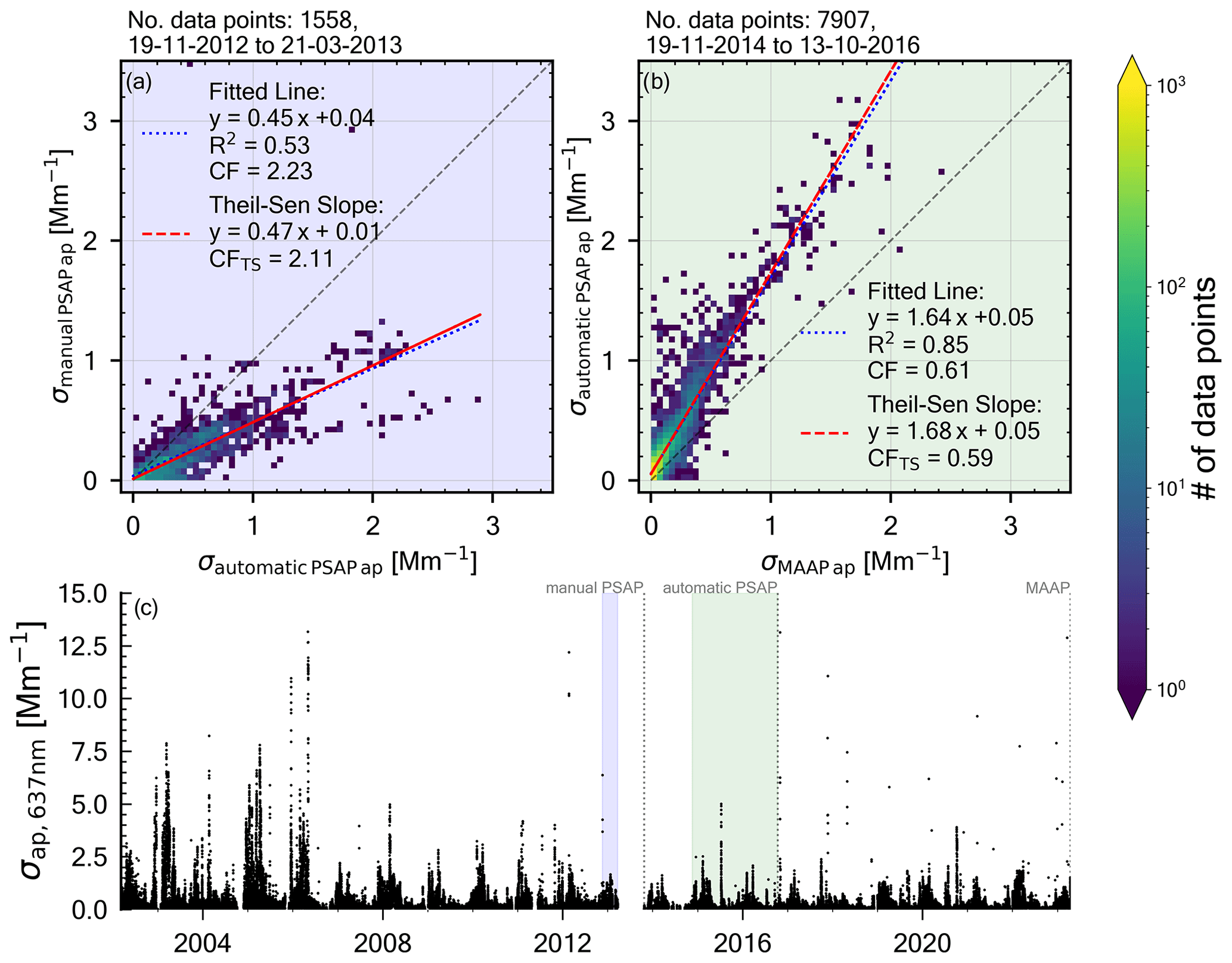
Figure 1Harmonisation of the long-term absorption coefficient (σap) data set: density plot shaded in blue in the top left corner (a) displaying the intercomparisons performed between the manual PSAP and automatic PSAP. The results of both the Theil–Sen slope estimator (TS) and least mean square (LMS) approach are displayed in the top left of the panel. (b) Density plot shaded in green, in the top right corner, displaying the comparison between the automatic PSAP and the MAAP. Both TS and LMS are displayed in the top left of the panel. (c) The time series of homogenised σap measured at 637 nm. The shaded stripes in (c) denote the respective period in which the instruments were measuring at the same time and comparisons between the respective data sets could be made. The dashed vertical line denotes the end time of each respective instrument. Note that the correction factor (CF) for the manual PSAP vs. automatic PSAP is not the CF that is applied to the data. The CF used in this case is the CF generated by comparing the σap from the manual PSAP with the corrected automatic PSAP σap.
2.2.4 Trend analysis
Aerosol optical properties are typically not normally distributed, and as a result, many statistical methods are not suitable for analysis of scattering and absorption data; observations of σap and σsp are better represented by log-normal distributions (Collaud Coen et al., 2020a). Medians are utilised for the trend analysis of σap and σsp because of the non-Gaussian nature of the data distribution and the fact that the use of medians is more robust against outliers. For all other variables though, including the accumulated back-trajectory precipitation (ATP), number of active fires, and emissions of black carbon, the arithmetic mean is utilised to perform the trend analysis.
In accordance with previous trend analysis studies (Collaud Coen et al., 2020a, 2013; Asmi et al., 2013), the Mann–Kendall test, seasonal Mann–Kendall test (hereafter “MK test” and “seasonal MK test”), and Theil–Sen estimator (TS) are utilised to estimate the statistical significance (SS) and magnitude of various long-term trends. The MK is performed on a two-tailed significance test of 95 % to ascertain the SS. The MK test and TS are nonparametric and are thus suitable for use with σap and σsp. A combination of daily, monthly, and seasonal arithmetic means and medians is used throughout the study to provide a range of resolutions that incorporate a range of data amount and degrees of autocorrelation. For daily averages, when the data are more likely to be plagued by autocorrelation, the data are “pre-whitened” using the three pre-whitening method (3PW) (Collaud Coen et al., 2020b). In keeping with similar studies (e.g. Collaud Coen et al., 2020a), daily averages were computed with the requirement that at least 25 % of the day consists of valid data (i.e. ∼ 6 h). For more details about TS see Sen (1968); for the MK test see Hirsch et al. (1982) and Gilbert (1987). The MK tests performed in this study made use of the Python package mannkendall v1.0.0 (https://doi.org/10.5281/zenodo.4134435 Collaud Coen et al., 2020b).
It should be noted that a single linear trend cannot fully capture the fate of light-absorbing aerosol in such a complex region. However, linear trends to simplify long-term changes have been used previously (e.g. Stone et al., 2014; Hirdman et al., 2010; Schmale et al., 2022; Collaud Coen et al., 2020a). Here, they are used to allow for greater exploration and interpretation.
2.3 Aerosol origin and transport
2.3.1 Transport model
The history of air masses arriving at ZEP was analysed using the Hybrid Single-Particle Lagrangian Integrated Trajectory model (HYSPLIT V5.2.1) (Draxler and Hess, 1998; Stein et al., 2015). An ensemble of 27 back trajectories was initialised for every hour. The ensemble was generated by offsetting the meteorological fields in all possible combinations of x and y; a grid of three planes, consisting of nine starting points, where each plane is ± 0.1 sigma (∼ 250 m) apart, was configured. The air parcels in the model arrive at an altitude of 250 m above the ground to avoid any issues related to the displacement of the ensemble members. The back trajectories were run for 10 d back in time, a compromise between capturing potential source regions and reducing the increased uncertainty generated by longer-run back trajectories. It should be noted that there was a change in the meteorological database used for the HYSPLIT back trajectories (end of 2004). The choice of input meteorological fields is considered the most important factor contributing to uncertainties (Dadashazar et al., 2021; Gebhart et al., 2005). The meteorological fields were obtained from the National Oceanic and Atmospheric Administration (NOAA); the period 2002–2004 uses the FNL (Final) Operational Global Analysis archive data from the National Weather Service's National Centers for Environmental Prediction (NCEP), and 2005–2023 uses the Global Data Assimilation System (GDAS) 1∘ × 1∘ archive data (http://ready.arl.noaa.gov/archives.php, last access: 7 December 2023). GDAS has been used in previous analyses of ZEP (e.g. Tunved et al., 2013). For the analysis here, a 1∘ × 1∘ rotated grid was initialised such that ZEP acted as the new north pole. To obtain continuous coverage of surface precipitation along the air mass transport pathway and prevent issues related to the change in meteorological fields (i.e. FNL to GDAS), the back trajectories were temporally and spatially collocated with fifth-generation ECMWF reanalysis (ERA5) hourly surface-level data (Hersbach et al., 2018) such that each end point (i.e. points along the back trajectories) was matched with the total surface precipitation variable from ERA5 for their respective geographical and temporal position. As a result, the precipitation variable is a product of the spatial coordinates of the HYSPLIT model runs using FNL (i.e. 2002–2004) and GDAS (i.e. 2005–present) as well as the surface precipitation data from ERA5. The accumulated surface precipitation was calculated by integrating along the back trajectory; hereafter, this parameter will be referred to as the accumulated trajectory precipitation (ATP) (a comparison of the GDAS–FNL and ERA5 ATP monthly medians can be found in Fig. S5 in the Supplement). The Python package PySPLIT (Cross, 2015) was used to generate the ensemble back trajectories.
2.3.2 Air mass backward-trajectory analysis
Back trajectories were classified into different air transportation pathways using a k-means clustering method. The sklearn.cluster Python package is used within scikit-learn v.1.2.1 (Pedregosa et al., 2011). The k-means clustering algorithm was performed on coordinates transformed from geographic coordinates (i.e. latitude, longitude, and altitude) to their equivalent Cartesian coordinates (i.e. ). The k-means clustering was performed on back-trajectory ensembles (i.e. 27 back trajectories per hour). Furthermore, the data were temporally collocated with the absorption coefficient data set such that only time stamps in which both data sets had valid data were used. In order to assign a cluster to each measurement a criterion was imposed such that more than 50 % of the 27 ensemble members had to have been assigned the same cluster. By specifying this criterion, 90 % of the data remained and ensembles with a mixed back-trajectory and air mass origin are removed (see Fig. S6). Identifying the transportation pathways enables trends of specific regions to be explored in more detail and for certain rain–aerosol relationships to be more closely analysed. Furthermore, the back trajectories were utilised to develop a concentration-weighted trajectory (CWT) in line with Seibert et al. (1994), Hsu et al. (2003), and Yan et al. (2015). This enabled a spatial overview of the various source regions. However, there is still the possibility that, given the spatial limitations, various source regions are beyond the reach of 10 d back trajectories.
2.3.3 Season definition
Arctic aerosol seasons are defined to account for the pronounced seasonality in aerosol concentrations measured at ZEP; the seasons are used throughout this study and are defined as follows.
-
Arctic haze (AHZ), February–May. AHZ involves enhanced concentrations of accumulation-mode aerosol. Transport is characterised by low amounts of precipitation, on average 2–3 mm of rain experienced by air masses during the 10 d prior to arrival (Tunved et al., 2013).
-
Summer (SUM), June–September. Decreased concentrations of accumulation-mode aerosol particles and enhanced concentrations of Aitken- and nucleation-mode particles characterise summer months. SUM experiences the highest amounts of precipitation, on average 7–8 mm of rain prior to arrival (Tunved et al., 2013).
-
Slow build-up (SBU), October–January. SBU is characterised as a transition period, in which the concentration of accumulation-mode particles begins to increase towards the end of the season, “building” back up to the concentrations observed during the AHZ seasons. The SBU season experiences little sunlight, with the polar night starting in November and ending in late January.
2.3.4 Forest fire identification
The Global Emission Fire Database (GFED) combines information from different satellite and in situ data (Van Der Werf et al., 2017). The fourth version with small fires, i.e. GFED4s, is used in partnership with the HYSPLIT back-trajectory data to estimate the fires and subsequent BC emissions which could potentially be transported to ZEP. In addition to GFED, the number of active forest fires recorded by MODIS was used to provide a fire count for each back trajectory. For the GFED, it was combined with HYSPLIT by summing up the emissions of BC within each traversed grid cell. The number of active fires was combined with HYSPLIT by summing up the number of active fires within each 1∘ × 1∘ grid and then counting the number of total active fires for each grid a back trajectory traversed whilst in the mixing layer, as defined by the HYSPLIT model (see example in Fig. S7). Li et al. (2020) found large uncertainties predicting the effects of BB effects with trajectory models; however, they noted that the use of ensemble means displayed the best performance.
3.1 Long-term trends in absorption coefficient and single-scattering albedo
Overall, the last 22 years of observations (2002–2023) have displayed a statistically significant decreasing trend in σap. The long-term trend, based on seasonal medians, is approximately −0.004 Mm−1 yr−1, whilst the trend based on daily medians corresponds to an SS of −0.002 Mm−1 yr−1; the pre-whitened trend (i.e. correcting for autocorrelation) is −0.0006 Mm−1 yr−1 (see Fig. 2). In relative terms (i.e. the ratio of the trend over the average), the rate of decline in σap corrected for autocorrelation corresponds to −0.82 % yr−1. All seasons experience decreasing trends of −0.001 Mm−1 yr−1 once corrected for autocorrelation. The relative trends are −0.793 % yr−1, −1.226 % yr−1, and −1.793 % yr−1 for the seasons AHZ, SBU, and SUM, respectively. The fact that all seasons display negative trends suggests that the Arctic haze is not the only season which experiences the influence of long-range air pollution. It is interesting to note that reduction in σap has not been consistent, and in fact we report an AHZ minimum of ∼ 0.02 Mm−1 in σap between 2016 and 2017. Thus to aid in the interpretation we can divide the time series into two periods: 2002–2016 and 2016–2023. The more recent period, 2016–2023, is characterised by an increasing tendency during the Arctic haze season of 0.004 Mm−1 yr−1 (see Fig. S8 in the Supplement. This shift in sign with the general reduction in the rate of decrease has been referred to as a “stagnation” (Schmale et al., 2022). The single-scattering albedo experienced an increase in the period from 2002 to 20, from 0.9 to close to 1 (see Fig. S9 in the Supplement). During this period of time, the increase in the SSA is a combination of a long-term increase in σsp (Heslin-Rees et al., 2020) and a decrease in σap (as presented here).
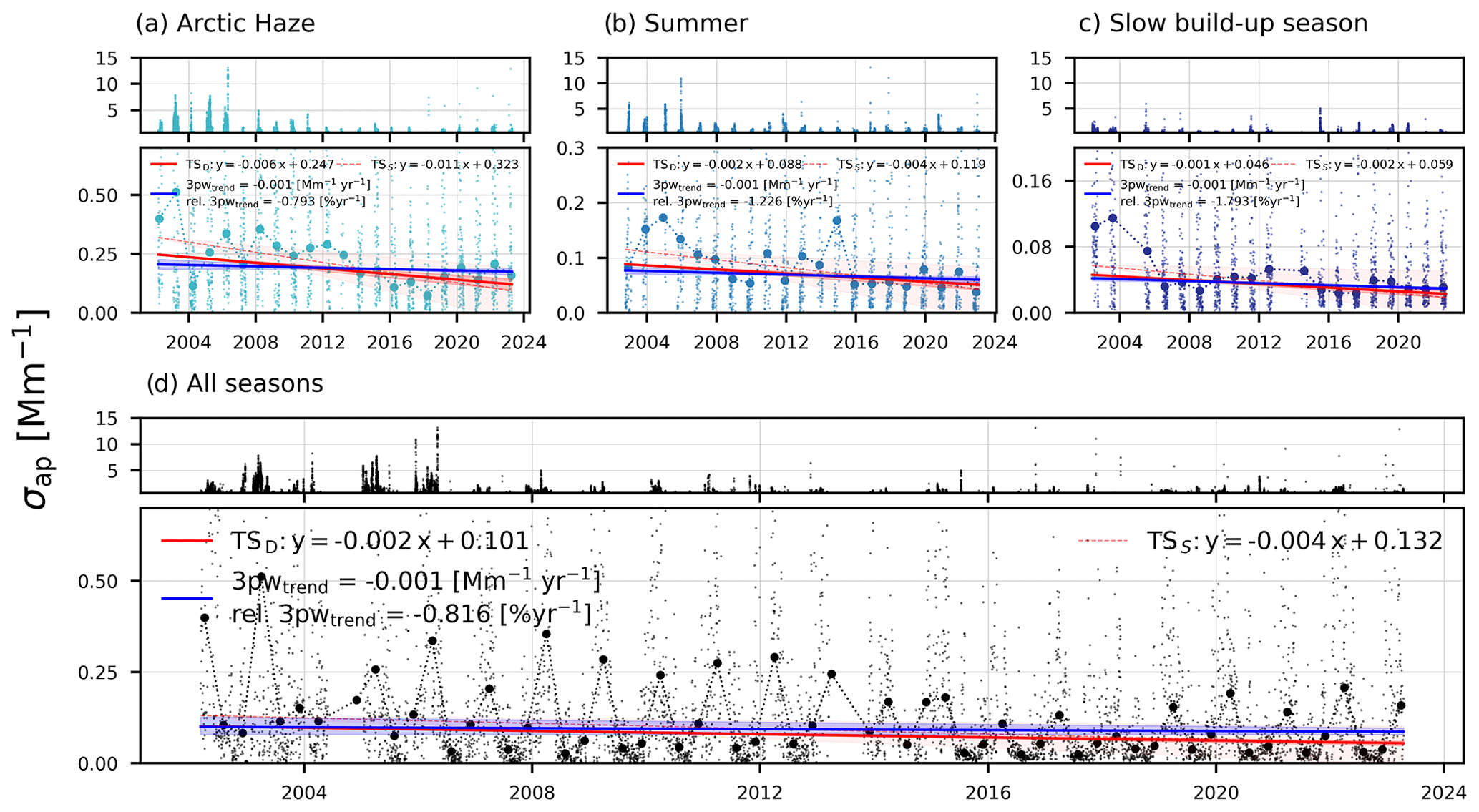
Figure 2Harmonised time series for the absorption coefficient (σap) measured at Zeppelin Observatory for the (a) Arctic haze season (February to May), (b) summer (June to September), (c) slow build-up season (October to January), and (d) the whole time series. The panels are split into two to display values greater than the maximum of the panel below. Both daily and seasonal medians are displayed in their respective colours; a colour represents each season, whilst black represents all seasons present. The trends for both daily (solid) and seasonal (dashed) medians are presented as red lines. The seasonal trends are homogeneous at the 83 % confidence limit (Gilbert, 1987; Sirois, 1998). The 3PW was performed using mannkendall v1.0.0. The trends for panels (a), (b), and (c) are the following: (a) Arctic haze – TS + 0.247, TS + 0.323, with 3PW Mm−1 yr−1 and relative 3PW % yr−1; (b) summer – TS + 0.088, TS + 0.119, with 3PW Mm−1 yr−1 and relative 3PW % yr−1; and (c) slow build-up – TS + 0.046, TSS = −0.002x + 0.059, with 3PW Mm−1 yr−1 and relative 3PW % yr−1.
3.2 Sources, sinks, and transport
Concentration-weighted trajectory (CWT) mappings are used to identify potential source areas (Hsu et al., 2003); σap measured at ZEP is weighted based on the time back trajectories spend traversing each grid cell within the mixing layer. CWT mappings possess information on sources, sinks, and transport. Grid cells with higher CWT values suggest that air masses from these areas contribute more to the absorption coefficient measured at ZEP. It is apparent that regions around north-central Eurasia contribute the most to the measured σap; however, there is a great deal of interannual variability in the magnitude and spatial distribution of CWT values (see Fig. S10 in the Supplement presenting the CWT mappings for each year). We have performed a spatial and temporal trend analysis of the CWT mappings (see Fig. 3). Essentially, the trend is calculated for each and every grid cell on an annual resolution.
Figure 3 signifies that the largest declines in the CWT value during the last 2 decades occurred in central Russia. Furthermore, we can ascertain that the long-term trends in the CWT value are mainly negative, with a slight increase in the contribution originating either in south-eastern Europe (i.e. regions neighbouring the Caspian and Black seas) or beyond. We argue that despite the limitations and uncertainties in the use of HYSPLIT, the overall spatial trends displayed in Fig. 3 resemble the trends in the emission inventories (see Fig. S11). In Fig. 3, regions furthest from ZEP can be expected to exhibit the largest uncertainties due to the increased length of time the model is run. Furthermore, we cannot exclude the influence of sources which are beyond the 10 d of transport modelled by HYSPLIT.
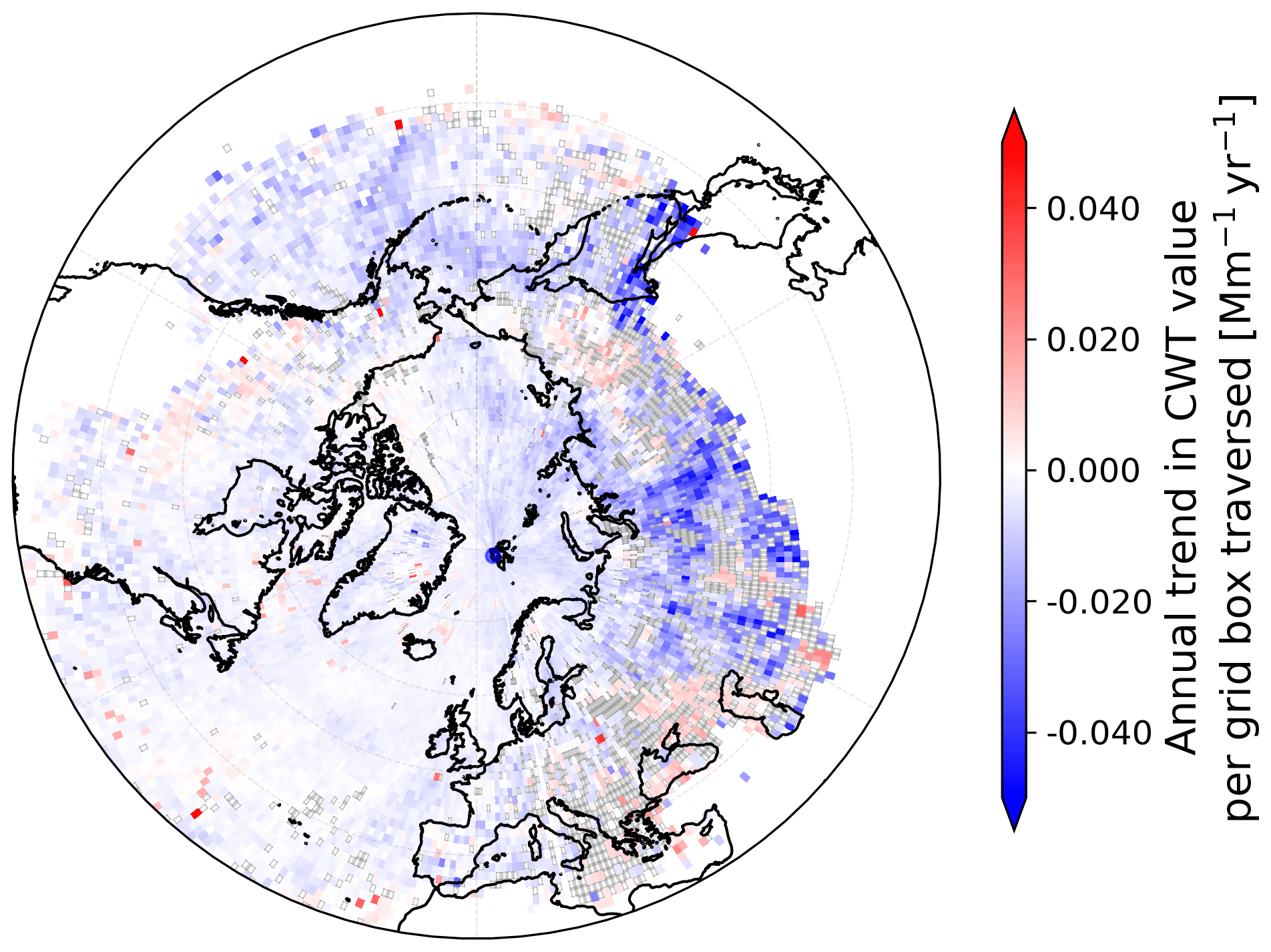
Figure 3Long-term trend in the annual CWT values for σap for the years 2002–2022 (the last year is not included as it is not a full year). A threshold of 15 data points for each 1∘ × 1∘ grid cell is applied to the mapping. All grid cells are statistically significant (p<0.05), unless the grid cell includes a grey border in which case it is not statistically significant. Statistical significance is determined by the 3PW method (Collaud Coen et al., 2020b). A confidence limit of 95 % is applied to the data.
The Eurasian continent has been shown to be one of the most important contributors to σap measured at ZEP (see Fig. S10), a finding which is in agreement with multiple other studies (Hirdman et al., 2010; Backman et al., 2014; Stathopoulos et al., 2021). The fact that this region contributes most to observations of σap is the result of a combination of source strength, air mass transport, and removal processes. For example, during the Arctic haze season, air masses coming from the direction of Siberia and Eurasia are more frequent (see Fig. S12) and are able to transport pollutants effectively to the Arctic. An area of particular interest is the Yamal–Nenets gas flaring region in central Russia; this potential source appears in Fig. S10, where there are elevated CWT σap values (AMAP, 2015; Stohl et al., 2013; Klimont et al., 2017; Stathopoulos et al., 2021). It also appears to be one of the regions exhibiting the largest reductions in CWT σap values (see Fig. 3). Klimont et al. (2017), based on the ECLIPSE V5a emission inventory, noted that emissions of BC decreased in regions affecting the Arctic such as western Europe, the USA, and the Russian region including several former Soviet Union countries (i.e. “Russia+”) in the period 2000 to 2010, with Russia+ exhibiting one of the largest relative reductions. Previous analysis of long-term trends has suggested that the declines in wintertime BC in the Arctic are the result of emissions changes in the former Soviet Union (Sharma et al., 2013), despite increasing BC emissions from source regions such as East Asia. In this work, we have seen that the spatial trends related to the CWT maps display large reductions for the central Russian region, whilst south-eastern Europe experiences increased CWT σap values (see Fig. 3). The positive trend in south-eastern Europe could be explained by increases in BC emissions, based on emission inventories from 2000 to 2010, in central Europe and nearby regions (e.g. Turkey, the Middle East, and parts of central Asia) (i.e. “Asia-Stan” as described in Klimont et al., 2017). This can also be seen in the trend analysis of the ECLIPSE V6b global emission inventories (see Fig. S11 in the Supplement or the spatial changes in emissions in AMAP, 2021). In regards to the CWT trends in Fig. 3, another possible explanation for the increase displayed in the region south-east of Europe could be changes to the contributions from sources further south (e.g. emissions from the Indo-Gangetic Plain over central Asia and into the high Arctic; Backman et al., 2014).
3.3 Transport
3.3.1 Trajectory source analysis
The clusters, with a total of five different clusters each signifying a potential transport pathway, are shown in Fig. 4. Typically, air masses arriving from Siberia (cluster 4 in Fig. 4) and Eurasia (cluster 5 in Fig. 4) exhibit the highest average concentrations of σap, with average values corresponding to 0.14 and 0.20 Mm−1, respectively. The Arctic Ocean cluster (3) is the most frequent, arriving approximately 31 % of the time. It is followed by the Siberia cluster (4) at 29 %, the North Atlantic cluster (1) at 19 %, and clusters 2 and 5 contributing to 11 % of the air masses. These average contributions vary throughout the year. The NA cluster is most present during the summer months (i.e. JJA), coinciding with reduced concentrations in σap observed on an annual basis. The Siberian cluster increases its contribution during the Arctic haze season (i.e. February to May) and decreases its contribution in SUM. The Eurasian cluster is most frequently present during the transition season and the start of the AHZ season (i.e. DJF). See Fig. S12 in the Supplement for more details on the seasonality of the clusters.
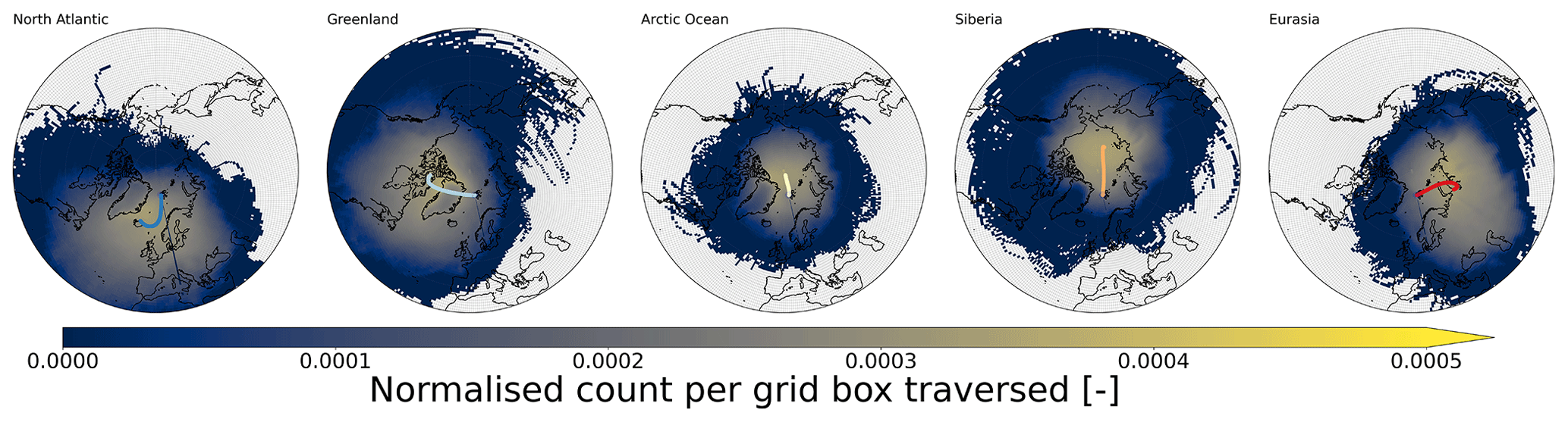
Figure 4Cluster analysis performed using the latitude, longitude, and altitude (converted to their equivalent Cartesian coordinates, i.e. ) of all data points in the collocated data set. The length of each back trajectory was set at 10 d. The centroids are shown in each cluster's respective colours. The centroids are arithmetic means of the respective Cartesian coordinates for each end point along a back trajectory. The mappings are normalised by dividing by the sum of the entire number of end points. The clusters are labelled based on their respective origins (clockwise direction based on the longitude of the last centroid endpoint): cluster 1 corresponds to the North Atlantic (NA) denoted by dark blue, cluster 2 to Greenland (G) denoted by light blue, cluster 3 to the Arctic Ocean (AO) shown in yellow, cluster 4 to Siberia (S) shown in orange, and cluster 5 to Eurasia (E) displayed in red.
By analysing the long-term trends in σap for the five clusters, we can observe that all of the clusters, except the Eurasian cluster, display a similar decreasing trend in σap (i.e. ∼ −0.003 Mm−1yr−1 for clusters 1–4) (see Fig. S13 in the Supplement for the trend in the Eurasian cluster). The Eurasian cluster, i.e. cluster 5, is the only transportation pathway which displays a positive trend in terms of seasonal medians, roughly 0.002 Mm−1 yr−1. This is in agreement with the CWT trend analysis (see Fig. 3 in Sect. 3.2), which shows that south-eastern Europe and also central Asia are among the few regions where there is an increasing trend in terms of contributions to σap measured at ZEP.
3.3.2 Trends in transport pathways
We can look at the frequency of the five clusters over the time span of 2002–2023, and in regards to changes in transportation, we can see that the frequency of various air masses arriving at ZEP has transitioned (see Fig. 5b). Most prominently, the North Atlantic and Greenland clusters have increased in their respective contributions; both of these transportation pathways are associated with little anthropogenic influence and therefore contribute to lower values of σap at ZEP. For example, the NA cluster is one of the cleanest air masses (with a median of 0.045 Mm−1). There is also an increased contribution from the Eurasian cluster (5), bringing air masses more influenced by anthropogenic sources; the Eurasian air masses exhibit the largest mean σap values and have increased their contribution from 15 % to 22 %.
Figure 5a is based on the same approach used in Hirdman et al. (2010); a fixed absorption coefficient value, based on the first 3 years of data, is assigned to each cluster, i.e. . The fixed values, , for each respective cluster are as follows: = 0.21 Mm−1, = 0.22 Mm−1, = 0.21 Mm−1, , = 0.42 Mm−1, and = 0.69 Mm−1). To estimate the influence of changing transportation pathways, a predicted σap is calculated by weighting each by their normalised frequency of occurrence. The long-term annual trend based on perturbing the fixed mean values, , in accordance with the changing relative proportions of each cluster is effectively zero (∼ 0.00031). The annual trend in the mean observed σap, however, shows a decreasing trend of −0.013 Mm−1. Note that along with Hirdman et al. (2010), the calculations here are based on the use of arithmetic means, which are more sensitive to outliers, as opposed to medians.
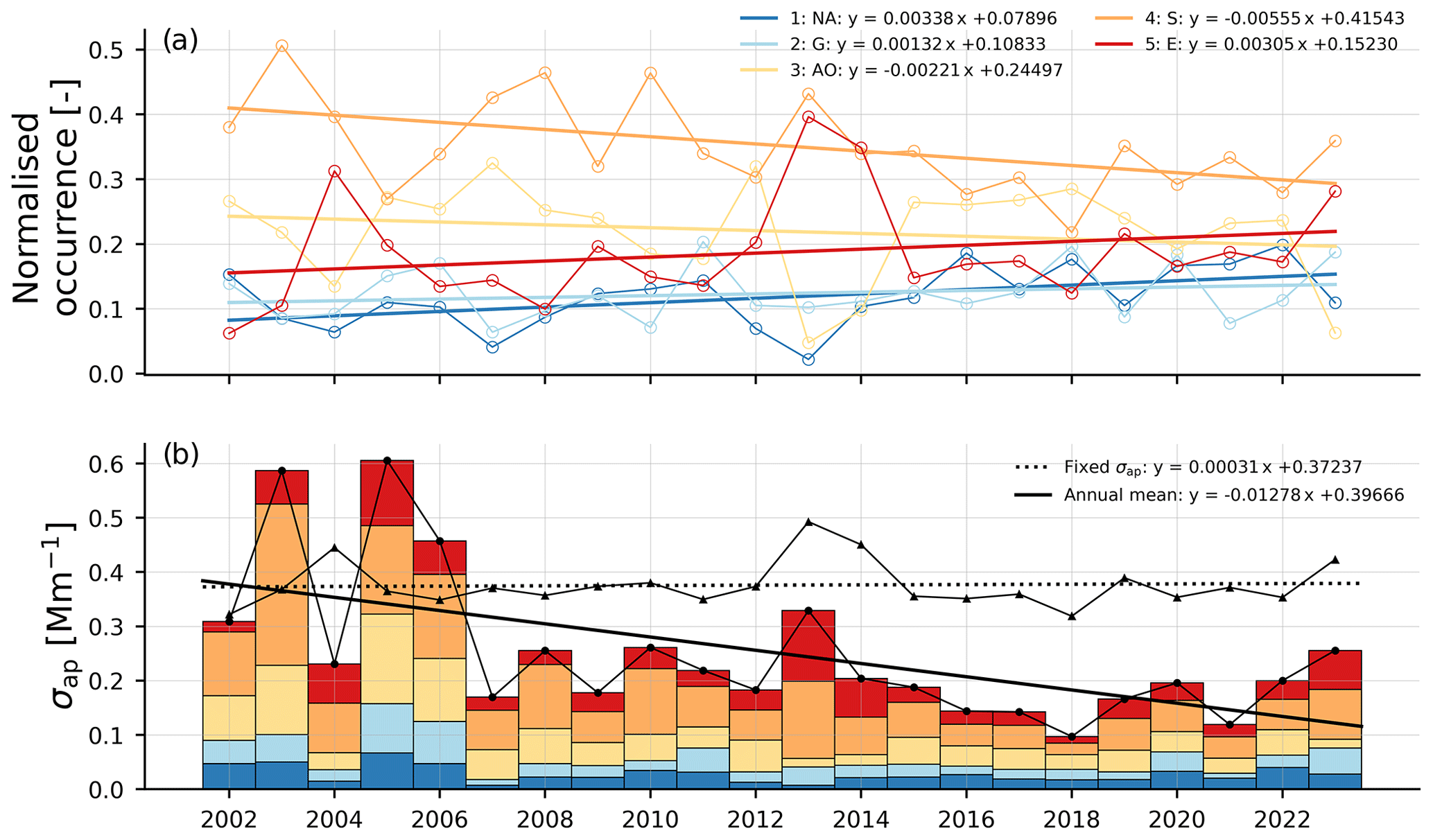
Figure 5The annual trends in (a) the occurrences of each respective cluster (1–5) and (b) the mean absorption coefficient (σap) estimated using the least mean square (LMS). Cluster 1 corresponds to the North Atlantic (NA) denoted by dark blue, cluster 2 to Greenland (G) denoted by light blue, cluster 3 to the Arctic Ocean (AO) shown in yellow, cluster 4 to Siberia (S) shown in orange, and cluster 5 to Eurasia (E) displayed in red. In (b) the height of each bar represents the annual mean σap and is subdivided based on the occurrence of each respective cluster. The dashed line describes the trend that would be associated with σap if fixed initial values were used and were only perturbed based on the changes in the frequency of occurrence of the various clusters.
In line with Hirdman et al. (2010), we argue that the changes in the various frequencies of different transportation pathways (i.e. clusters) are not a controlling factor explaining the reduction in σap. One possible reason for this may be the fact that there is a compensating effect taking place, where despite an increased contribution from cleaner air masses (i.e. Greenland and the North Atlantic), there is also an increased contribution from air masses from high-emission regions (i.e. Eurasia). In regards to the increased single-scattering albedo measured at ZEP, this could still be the result of an increased contribution of marine air masses, which bring with them sea spray aerosol consisting of an SSA close to unity. Previous studies have suggested that this increase in the contribution of more marine air masses is likely the result of changes in air circulation patterns (Heslin-Rees et al., 2020). In regards to changes in large-scale circulation patterns, additional studies have shown that the phase of the Scandinavian pattern can affect the variability in transported BC (Stathopoulos et al., 2021); during the cold period and when the Scandinavian pattern (SCAN) is in its negative phase, higher concentrations of BC were present when sources were limited to more northern regions (e.g. the Yamal gas flaring region), as opposed to during SCAN+ when source regions extended further south, were more diffused, and potentially experienced more wet removal.
3.4 Sinks and transport
Light-absorbing aerosol can be removed from the atmosphere via the process of wet deposition; there are two mechanisms by which these aerosol particles are removed: in-cloud scavenging and below-cloud scavenging (Pruppacher and Klett, 2010; Zieger et al., 2023). In-cloud scavenging occurs when aerosols act as CCN, forming cloud droplets, or when aerosols collide with preexisting droplets. Below-cloud scavenging describes the removal of ambient aerosol by falling hydrometers. Here, we focus on precipitation, in particular accumulated precipitation along the back trajectories, with the assumption that aerosols en route to ZEP, which have acted as CCN, are removed. For below-cloud scavenging, there is the chance that the impact of ATP is overestimated as aerosol particles can be above cloud height; however, ATP can also be underestimated if precipitation fails to reach the surface. This type of analysis places the focus on the removal of aerosol from the atmosphere, without emphasis on whether it is necessarily driven by in-cloud or below-cloud scavenging. Precipitation scavenging is assumed to act as a sink of aerosol.
3.4.1 Trends in precipitation
The overall trend in mean accumulated back-trajectory precipitation (ATP) using the 3PW method is statistically significant, positive, and approximately 0.028 mm yr−1 (p∼0.009), representing a relative annual increase of ∼ 0.35 % yr−1 (see Fig. 6). The most significant increase in average accumulated precipitation occurred during 2002–2012. After 2014, the positive trend in accumulated precipitation appears to have stagnated or shown a slight decline. We conclude that the air masses arriving at ZEP have witnessed increased surface precipitation, a finding that is related to an increase in the amount of precipitation and not that air masses en route to ZEP are spending more time at lower and wetter latitudes. The finding that the air masses en route to the Arctic have experienced an increase in accumulated precipitation is in agreement with previous studies showing that the Arctic is getting wetter (Bintanja, 2018; Yu and Zhong, 2021). The periods that experienced the largest reductions in seasonal average σap coincided with periods experiencing increasing ATP. The period in which σap declines the least (if not increases) occurs during a period of little change to ATP (i.e. 2016 onwards for σap).
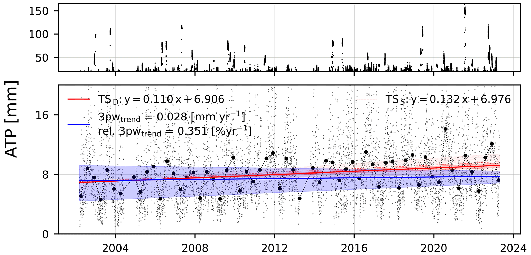
Figure 6Time series of average accumulated precipitation experienced by 10 d back trajectories arriving at ZEP. The precipitation at the surface is taken from ERA5 reanalysis. The data are not selected such that the air mass is within the mixing layer; instead it is assumed the air mass is influenced by the precipitation regardless of altitude. The seasonal trends are homogeneous at the 80 % confidence limit, with the use of mannkendall v1.0.0.
Extreme-ATP events (ATP values, after applying a 15 d rolling 99th percentile to the data set) increased over time as well; approximately 18 % of the clean days (i.e. days on which σap was within the 1st percentile) coincided with days with exceptionally high ATP (i.e. 99th percentile). This suggests that extreme amounts of rainfall during the air mass transport to ZEP are an explanation for a significant number of the exceptionally low σap values (see Fig. S15). Extreme accumulated precipitation events can have a meaningful impact on the overall arithmetic mean σap such that when periods coinciding with high-ATP events are removed from the data set, the mean σap increases. However, in terms of trends it has been seen that extreme precipitation events do not dictate the trends (not shown here); all trend analyses that utilised daily medians (as opposed to arithmetic means) seemed to be quite robust to the removal of extreme-ATP periods.
To gauge the extent to which the aforementioned increasing trend in accumulated back-trajectory precipitation (ATP) can influence σap, the trend in σap was recreated. The variable , denoting a calculated σap as opposed to an observed σap, was produced. uses the dependency between σap and ATP to map the ATP variables onto values. The dependency between σap and ATP reflects the influence of precipitation scavenging and was analysed for all three seasons (AHZ, SUM, and SBU) and all five source regions (NA, G, AO, S, and E) such that 15 empirical relationships were ascertained (see Fig. S17). Essentially, cluster- and season-specific relationships for σap and ATP were utilised to try and simulate the long-term trend in σap; the relation between ATP and the median σap was used on a seasonal basis to account for different precipitation regimes. For each cluster and for each season, every 1 or 2 mm of ATP was compared to its respective median σap value; linear interpolation was used to extend the resolution beyond 1 or 2 mm. The relationship between ATP and σap was developed using random samples of different fractions of the data set. The amount of data used (i.e. ≤ 50 % of the data) is a compromise between having enough data points for a robust analysis of the relationship and not using all of the data in the development of the parameterisation. For the majority of transportation clusters and seasons, σap decreases as ATP increases; however, the extent of the decline in σap as ATP increases varies depending on the cluster and season (see Fig. S17). It should be noted that a key assumption in these calculations is that σap is solely dependent on ATP and that there are no additional factors.
was able to mimic the seasonality in σap well, with the distinctive Arctic haze events towards the end of winter (when ATP is low). However, underestimated any large seasonal averages; regardless, the reproduced seasonality signifies that ATP is a major factor in controlling the annual cycle.
In terms of long-term trends, multiple subsamples of the data of varying length were used to generate time series. The trend analysis was performed on the pre-whitened time series, and the trend in the calculated absorption coefficient is compared with the 3PW trend for in situ measurements. Figure 7 shows decreasing trends in , suggesting that ATP plays a role in the decline in σap. The resultant average trend for is approximately −0.00016 Mm−1yr−1. Overall, the 22-year-long trend in was found to be dependent on the trend in ATP. The trend in the calculated σap, i.e. , was roughly 26 % of the magnitude of the trend in the in situ σap observations (i.e. −0.00016 Mm−1 yr−1 compared to the observed trend of −0.00064 Mm−1 yr−1).
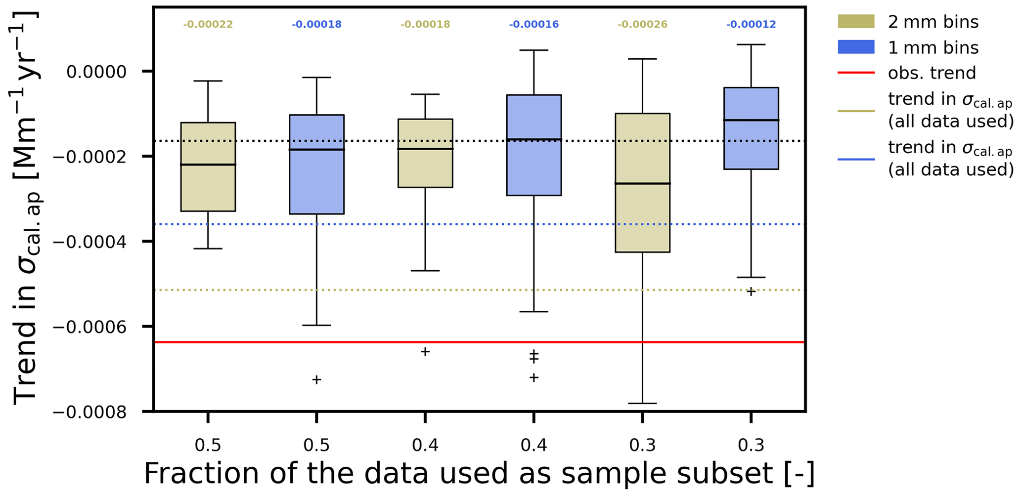
Figure 7The trend in the calculated after performing the analysis 50 times for a random subset of data. The trend is calculated using the 3PW method such that it is corrected for autocorrelation. The box plots are displayed as a function of the fraction of the data used for the subsampling and the size of the binning performed (i.e. median σap every 1 mm of ATP). The fraction of the data is displayed along the x axis, whilst the colour of the box plots signifies whether the data are binned per every 1 mm (blue) or every 2 mm (khaki). The long-term trend analysis was based on daily medians. The red line signifies the long-term trend for the observed absorption coefficient (σap). The khaki and blue lines correspond to the trend in the calculated absorption value (σcal.ap) if all the data are used (i.e. fraction = 1.0). The limits of the box are from the first quartile to the third quartile, with the line signifying the median. The whiskers extend to 1.5× the interquartile range (IQR). Outliers are marked by the + symbol and represent trends outside the extent of the whiskers. The values displayed above the boxes denote the median value of the respective box.
It is well documented that the distinct seasonality of aerosol particles in the Arctic is influenced by precipitation (Garrett et al., 2011; Tunved et al., 2013). Less precipitation is experienced by air masses during the Arctic haze season (see Fig. S14), meaning that the aerosol particles undergo less removal. Tunved et al. (2013) demonstrated that wet removal largely controls the aerosol size distributions observed in the Arctic. The summer generally exhibits the greatest amount of accumulated precipitation, while the Arctic haze season experiences the least. Furthermore, Tunved et al. (2013) noted that there is an exponential decrease in particle mass with accumulated precipitation; the reduction in mass is most apparent for the first few incremental increases in ATP (a finding also demonstrated in Fig. S17 in the Supplement where σap is also reduced with an increase in ATP, suggesting that light-absorbing particles are wet-scavenged effectively with the initial increases in ATP). We argue here that the increased precipitation experienced by air masses transported to ZEP has led to light-absorbing aerosol being more efficiently scavenged en route to the Arctic, thus resulting in a cleaner Arctic. In general, more work is required to see how different aerosol types and different types of precipitation can impact the degree of wet scavenging and hence estimated σap. Moreover, it should be noted that other parameters are important when analysing wet removal processes. The efficiency of wet deposition can depend on the temperature and type of precipitation, not only the amount; for example, wet deposition efficiency is lower in winter as snow is less effective at removing BC than rain (Croft et al., 2009). Another aspect depends on the hydrophilic fraction of BC. As BC ages, it changes from hydrophobic to hydrophilic. If BC ages more slowly as it is transported to the Arctic, it could mean that the hydrophobic fraction will be larger, and thus it may be less effectively scavenged en route to the Arctic. For a more rigorous analysis, additional parameters that affect wet scavenging, such as temperature (above 0 ∘C), relative humidity, precipitation type, cloud phase, and aerosol chemical composition, need to be taken into account as it is not only ATP that controls wet scavenging. The work by Zieger et al. (2023) at the same observatory showed, for example, that the ability of eBC to be incorporated into cloud droplets via nucleation scavenging was positively correlated with cloud water content and was reduced at low temperatures. Reduction in sources is often mentioned as the only factor controlling long-term reductions in BC in the Arctic (Stohl et al., 2013), despite wet scavenging commonly being cited as the controlling factor when it comes to the distinct seasonality seen in the Arctic (Garrett et al., 2011; Shen et al., 2017; Tunved et al., 2013).
3.5 Sources and transport
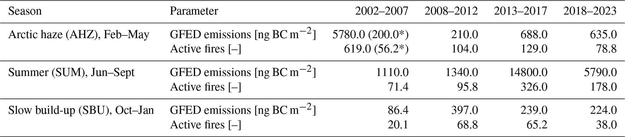
Wildfires have led to an increase in BC emissions in the Arctic in recent years (McCarty et al., 2021), and it has been suggested that forest fires are also becoming more frequent and severe (Rogers et al., 2020). This source of BC has been shown to dominate the σap measurements during summer (Winiger et al., 2019); however, it remains unknown whether or not this dominance during the summer is a new phenomenon (Schmale et al., 2022). The air masses arriving at ZEP have experienced an increasing influence from active forest fires during the study period (see Table 1). The average number of active forest fires each back trajectory traversed has increased since 2002, with the most notable shift occurring after 2015. The same can be said for biomass burning BC emissions based on the GFED. Stathopoulos et al. (2021) observed from their analysis of aerosol light-absorbing carbon from 2001–2015 that emission rates from open fires increased by factors of between 3.4 and 3.6 for the warm period (May–October) for the years 2006–2010 and 2011–2015 relative to 2001–2005.
Table 1Seasonal arithmetic means for the accumulated black carbon (BC) emissions and the accumulated number of active fires along the 10 d back trajectories. The BC emissions are defined by the Global Fire Emission Database (GFED), which has a spatial resolution of 0.25∘. From 2003, GFED operated on a 3-hourly resolution (emissions were divided by 3 to collocate the one-ensemble per hour back trajectories). The number of active fires is based on a constructed 1∘ × 1∘ grid of the active fire frequency. The number of active fires is taken from MODIS and is of X resolution. Only air masses within the mixed layer along the back trajectories are selected and counted. The asterisks (*) signify the seasonal average if the 2006 agricultural fire is removed, i.e. between 21 April 2006 and 7 May 2006 (Stohl et al., 2007).
There are several examples of high-σap-concentration episodes observed at Arctic sites, caused by emissions from fires (e.g. Stohl et al., 2007; Markowicz et al., 2016). For the purposes of this study, extreme BB events were classified as such using a 15 d rolling 99th percentile of the BC emissions from GFED (similar methods were utilised by Della-Marta et al., 2007); the rolling percentile was applied to the data set representing the accumulated BC emissions from global fires. To explore the influence of these extreme BB events, the σap measurements coinciding with these BB events were removed from the data set. When measurements coinciding with these BB events were removed (∼ 3 % of the total number of σap data points), it was shown that these BB events could have a significant impact on seasonal summer mean σap values, in particular after 2014. By removing the extreme events the arithmetic σap mean is reduced by as much as ∼ 33 % for SUM 2015 (see Fig. S16 in the Supplement). The seasonal median σap values, however, were essentially unaltered by the removal of these time periods from the data set.
Despite the increase in BB and the related impact on the arithmetic seasonal means, the removal of periods corresponding to extreme BB events had no noticeable influence on the long-term σap trends (not shown here). The trend analyses in this study are based on medians and thus less sensitive to the influence of extreme events such as BB events, suggesting the trends are dictated by background conditions rather than sporadic but increasing extreme events. Schmale et al. (2022) suggested that another possible explanation for the lack of a BB signature in the long-term σap and eBC trends could be related to the height at which wildfire plumes are injected; BC from BB events could be emitted into the atmosphere further aloft and thus arrive at ZEP at higher altitudes, while still slowly filling the Arctic domain with biomass burning aerosol.
In this study, we have successfully harmonised absorption and scattering coefficient data at ZEP from 2002 to 2023. The length of the data set allows for a unique examination of long-term trends in aerosol optical properties in the Arctic. It represents one of the longest aerosol optical time series in the Arctic. We found that ZEP has experienced declines in σap in line with previous trend analysis studies which have detailed reductions in σap and/or eBC (Collaud Coen et al., 2020a; Schmale et al., 2022; Sharma et al., 2013; AMAP, 2015). In addition to the overall decreasing trend, we note that there has been a shift in the sign of the trend from negative to positive after σap displayed a minimum in 2016. In regards to the recent increasing σap tendency during the Arctic haze season, it is argued here that the recent increase in σap is the result of a combination of several factors: an increase in the frequency of occurrence of generally polluted air masses from Siberia, an increase in contributions from sources in the south-east of Europe or beyond, and a decline in the precipitation en route during the last 10 d of transport to Zeppelin station from 2015 onwards.
The aerosol properties were temporally collocated with the arrival time of the back trajectories to understand which atmospheric parameters were potential factors in influencing averages, seasonality, and overall long-term trends. Our analysis especially looks at the effect of accumulated precipitation and biomass burning events on the characteristics of atmospheric light-absorbing aerosol.
We conclude that the observed trends in σap are not the result of changes in the frequencies of certain transportation pathways due to the compensating nature of the five prevailing transportation pathways. Instead, we argue that changes in sources, along with increases in accumulated back-trajectory precipitation (ATP), have governed the decline in σap. In this study, we argue that increases in ATP have aided the reduction in light-absorbing aerosol concentrations, signifying a tendency towards a wetter, but cleaner, Arctic. It should be noted that if trends in wet scavenging were to increase in a warmer and wetter Arctic climate, then any further increases in ATP would result in a reduced impact on σap, as σap cannot be reduced further. Finally, in regards to additional sources of natural BC such as forest fires, these sources have shown that they can significantly alter seasonal means; however, trends remain robust to their increases in frequency.
The code for this study is available on GitHub via https://doi.org/10.5281/zenodo.10456676 (dominichr1, 2024).
The data from this study are available in the Bolin Centre Database (https://doi.org/10.17043/zeppelin-heslin-rees-2024-light-scattering-1, Heslin-Rees et al., 2024).
The supplement related to this article is available online at: https://doi.org/10.5194/acp-24-2059-2024-supplement.
DH-R, RK, and PZ together designed the study. DH-R performed data analysis and wrote the paper together with RK with input from PT, JS, PZ, IR, AK, PT, and JS. JS set up the custom-built PSAP at ZEP. RC ran back trajectories to 2020. KE provided Aethalometer data. All authors read and commented on the paper.
At least one of the (co-)authors is a member of the editorial board of Atmospheric Chemistry and Physics. The peer-review process was guided by an independent editor, and the author also has no other competing interests to declare.
Publisher's note: Copernicus Publications remains neutral with regard to jurisdictional claims made in the text, published maps, institutional affiliations, or any other geographical representation in this paper. While Copernicus Publications makes every effort to include appropriate place names, the final responsibility lies with the authors.
We would like to thank research engineers Birgitta Noone, Tabea Henning, and Ondrej Tesar from ACES and the staff from the Norwegian Polar Institute (NPI) for their on-site support. NPI is also acknowledged for substantial long-term support in maintaining the measurements at Zeppelin Observatory. We would also like to thank Kai Rosman for developing the software we used for the instrumentation at Zeppelin.
We thank the Norwegian Institute for Air Research (NILU) for providing the ambient meteorological data and for maintaining the EBAS database.
This research has been supported by ACTRIS–Sweden and the Horizon Europe EU Project FOCI (project 101056783), the Framework Programme Project FORCeS (grant agreement no. 821205), the European Research Council (Consolidator Grant INTEGRATE, agreement no. 865799), and the Knut and Alice Wallenberg Foundation (project grant ACAS, Wallenberg Scholarship AtmoCLOUD agreements nos. 2021.0169 and 2021.0298). The article processing charges for this open-access publication were covered by Stockholm University.
This paper was edited by Birgit Wehner and reviewed by two anonymous referees.
Acosta Navarro, J. C., Varma, V., Riipinen, I., Seland, Ø., Kirkevåg, A., Struthers, H., Iversen, T., Hansson, H.-C., and Ekman, A. M.: Amplification of Arctic warming by past air pollution reductions in Europe, Nat. Geosci., 9, 277–281, 2016. a
AMAP: AMAP assessment 2015: Black Carbon and Ozone as arctic climate forcers, Arctic Monitoring and Assessment Programme (AMAP), Oslo, Norway, https://www.amap.no/documents/doc/amap-assessment-2015-black-carbon-and-ozone (last access: 1 September 2023), 2015. a, b, c
AMAP: AMAP Assessment 2021: Impacts of Short-lived Climate Forcers on Arctic Climate, Air Quality, and Human Health, Arctic Monitoring and Assessment Programme (AMAP), Tromsø, Norway. x+ 375 pp., 2021. a, b, c, d, e
Anderson, T. L. and Ogren, J. A.: Determining aerosol radiative properties using the TSI 3563 integrating nephelometer, Aerosol Sci. Technol., 29, 57–69, 1998. a
Asmi, A., Collaud Coen, M., Ogren, J. A., Andrews, E., Sheridan, P., Jefferson, A., Weingartner, E., Baltensperger, U., Bukowiecki, N., Lihavainen, H., Kivekäs, N., Asmi, E., Aalto, P. P., Kulmala, M., Wiedensohler, A., Birmili, W., Hamed, A., O'Dowd, C., G Jennings, S., Weller, R., Flentje, H., Fjaeraa, A. M., Fiebig, M., Myhre, C. L., Hallar, A. G., Swietlicki, E., Kristensson, A., and Laj, P.: Aerosol decadal trends – Part 2: In-situ aerosol particle number concentrations at GAW and ACTRIS stations, Atmos. Chem. Phys., 13, 895–916, https://doi.org/10.5194/acp-13-895-2013, 2013. a
Asmi, E., Backman, J., Servomaa, H., Virkkula, A., Gini, M. I., Eleftheriadis, K., Müller, T., Ohata, S., Kondo, Y., and Hyvärinen, A.: Absorption instruments inter-comparison campaign at the Arctic Pallas station, Atmos. Meas. Tech., 14, 5397–5413, https://doi.org/10.5194/amt-14-5397-2021, 2021. a, b, c
Backman, J., Virkkula, A., Vakkari, V., Beukes, J. P., Van Zyl, P. G., Josipovic, M., Piketh, S., Tiitta, P., Chiloane, K., Petäjä, T., Kulmala, M., and Laakso, L.: Differences in aerosol absorption Ångström exponents between correction algorithms for a particle soot absorption photometer measured on the South African Highveld, Atmos. Meas. Tech., 7, 4285–4298, https://doi.org/10.5194/amt-7-4285-2014, 2014. a, b, c
Bintanja, R.: The impact of Arctic warming on increased rainfall, Sci. Rep., 8, 1–6, 2018. a
Bodhaine, B. A. and Dutton, E. G.: A long-term decrease in Arctic haze at Barrow, Alaska, Geophys. Res. Lett., 20, 947–950, 1993. a
Bond, T. C., Anderson, T. L., and Campbell, D.: Calibration and intercomparison of filter-based measurements of visible light absorption by aerosols, Aerosol Sci. Technol., 30, 582–600, 1999. a
Bond, T. C., Doherty, S. J., Fahey, D. W., Forster, P. M., Berntsen, T., DeAngelo, B. J., Flanner, M. G., Ghan, S., Kärcher, B., Koch, D., and Kinne, S: Bounding the role of black carbon in the climate system: A scientific assessment, J. Geophys. Res.-Atmos., 118, 5380–5552, 2013. a, b
Collaud Coen, M., Andrews, E., Asmi, A., Baltensperger, U., Bukowiecki, N., Day, D., Fiebig, M., Fjaeraa, A. M., Flentje, H., Hyvärinen, A., Jefferson, A., Jennings, S. G., Kouvarakis, G., Lihavainen, H., Lund Myhre, C., Malm, W. C., Mihapopoulos, N., Molenar, J. V., O'Dowd, C., Ogren, J. A., Schichtel, B. A., Sheridan, P., Virkkula, A., Weingartner, E., Weller, R., and Laj, P.: Aerosol decadal trends – Part 1: In-situ optical measurements at GAW and IMPROVE stations, Atmos. Chem. Phys., 13, 869–894, https://doi.org/10.5194/acp-13-869-2013, 2013. a
Collaud Coen, M., Andrews, E., Alastuey, A., Arsov, T. P., Backman, J., Brem, B. T., Bukowiecki, N., Couret, C., Eleftheriadis, K., Flentje, H., Fiebig, M., Gysel-Beer, M., Hand, J. L., Hoffer, A., Hooda, R., Hueglin, C., Joubert, W., Keywood, M., Kim, J. E., Kim, S.-W., Labuschagne, C., Lin, N.-H., Lin, Y., Lund Myhre, C., Luoma, K., Lyamani, H., Marinoni, A., Mayol-Bracero, O. L., Mihalopoulos, N., Pandolfi, M., Prats, N., Prenni, A. J., Putaud, J.-P., Ries, L., Reisen, F., Sellegri, K., Sharma, S., Sheridan, P., Sherman, J. P., Sun, J., Titos, G., Torres, E., Tuch, T., Weller, R., Wiedensohler, A., Zieger, P., and Laj, P.: Multidecadal trend analysis of in situ aerosol radiative properties around the world, Atmos. Chem. Phys., 20, 8867–8908, https://doi.org/10.5194/acp-20-8867-2020, 2020a. a, b, c, d, e, f
Collaud Coen, M., Andrews, E., Bigi, A., Martucci, G., Romanens, G., Vogt, F. P. A., and Vuilleumier, L.: Effects of the prewhitening method, the time granularity, and the time segmentation on the Mann–Kendall trend detection and the associated Sen's slope, Atmos. Meas. Tech., 13, 6945–6964, https://doi.org/10.5194/amt-13-6945-2020, 2020b. a, b, c
Croft, B., Lohmann, U., Martin, R. V., Stier, P., Wurzler, S., Feichter, J., Posselt, R., and Ferrachat, S.: Aerosol size-dependent below-cloud scavenging by rain and snow in the ECHAM5-HAM, Atmos. Chem. Phys., 9, 4653–4675, https://doi.org/10.5194/acp-9-4653-2009, 2009. a
Dadashazar, H., Alipanah, M., Hilario, M. R. A., Crosbie, E., Kirschler, S., Liu, H., Moore, R. H., Peters, A. J., Scarino, A. J., Shook, M., Thornhill, K. L., Voigt, C., Wang, H., Winstead, E., Zhang, B., Ziemba, L., and Sorooshian, A.: Aerosol responses to precipitation along North American air trajectories arriving at Bermuda, Atmos. Chem. Phys., 21, 16121–16141, https://doi.org/10.5194/acp-21-16121-2021, 2021. a
Dalirian, M., Ylisirniö, A., Buchholz, A., Schlesinger, D., Ström, J., Virtanen, A., and Riipinen, I.: Cloud droplet activation of black carbon particles coated with organic compounds of varying solubility, Atmos. Chem. Phys., 18, 12477–12489, https://doi.org/10.5194/acp-18-12477-2018, 2018. a
Dekhtyareva, A., Holmén, K., Maturilli, M., Hermansen, O., and Graversen, R.: Effect of seasonal mesoscale and microscale meteorological conditions in Ny-Ålesund on results of monitoring of long-range transported pollution, Polar Res., 37, 1508196, https://doi.org/10.1080/17518369.2018.1508196, 2018. a
Della-Marta, P. M., Haylock, M. R., Luterbacher, J., and Wanner, H.: Doubled length of western European summer heat waves since 1880, J. Geophys. Res.-Atmos., 112, D15, https://doi.org/10.1029/2007JD008510, 2007. a
dominichr1: dominichr1/ACP_DHR_2024: 1.1.1. In Increase in precipitation scavenging contributes to long-term reductions of light-absorbing aerosol in the Arctic, (1.1.1), Zenodo [data set], https://doi.org/10.5281/zenodo.10456676, 2024. a
Draxler, R. R. and Hess, G.: An overview of the HYSPLIT_4 modelling system for trajectories, Aust. Meteorol. Mag., 47, 295–308, 1998. a
Eleftheriadis, K., Vratolis, S., and Nyeki, S.: Aerosol black carbon in the European Arctic: measurements at Zeppelin station, Ny-Ålesund, Svalbard from 1998–2007, Geophys. Res. Lett., 36, 2, https://doi.org/10.1029/2008GL035741, 2009. a, b
Freud, E., Krejci, R., Tunved, P., Leaitch, R., Nguyen, Q. T., Massling, A., Skov, H., and Barrie, L.: Pan-Arctic aerosol number size distributions: seasonality and transport patterns, Atmos. Chem. Phys., 17, 8101–8128, https://doi.org/10.5194/acp-17-8101-2017, 2017. a
Garrett, T. J., Brattström, S., Sharma, S., Worthy, D. E., and Novelli, P.: The role of scavenging in the seasonal transport of black carbon and sulfate to the Arctic, Geophys. Res. Lett., 38, 16, https://doi.org/10.1029/2011GL048221, 2011. a, b, c, d, e, f
Gebhart, K. A., Schichtel, B. A., and Barna, M. G.: Directional biases in back trajectories caused by model and input data, J. Air Waste Manage. Assoc., 55, 1649–1662, 2005. a
Gilbert, R. O.: Statistical methods for environmental pollution monitoring, John Wiley & Sons, 1987. a, b
Hänel, G., Weidert, D., and Busen, R.: Absorption of solar radiation in an urban atmosphere, Atmos. Environ. B, 24, 283–292, https://doi.org/10.1016/0957-1272(90)90034-R, 1990. a
Hansen, J. and Nazarenko, L.: Soot climate forcing via snow and ice albedos, P. Natl. Acad. Sci. USA, 101, 423–428, 2004. a, b
Hersbach, H., Bell, B., Berrisford, P., Biavati, G., Horányi, A., Muñoz Sabater, J., Nicolas, J., Peubey, C., Radu, R., Rozum, I., Schepers, D., Simmons, A., Soci, C., Dee, D., and Thépaut, J.-N.: ERA5 hourly data on single levels from 1959 to present., https://doi.org/10.24381/cds.adbb2d47, copernicus Climate Change Service (C3S) Climate Data Store (CDS), 2018. a
Heslin-Rees, D., Burgos, M., Hansson, H.-C., Krejci, R., Ström, J., Tunved, P., and Zieger, P.: From a polar to a marine environment: has the changing Arctic led to a shift in aerosol light scattering properties?, Atmos. Chem. Phys., 20, 13671–13686, https://doi.org/10.5194/acp-20-13671-2020, 2020. a, b
Heslin-Rees, D., Tunved, P., Ström, J., Cremer, R., Zieger, P., Riipinen, I., Ekman, A., Eleftheriadis, K., and Krejci, R.: Light absorbing aerosol along with air mass history measured at the Zeppelin observatory in Svalbard. Dataset version 1, Bolin Centre Database, Stockholm University [code], https://doi.org/10.17043/zeppelin-heslin-rees-2024-light-scattering-1, 2024. a
Hirdman, D., Burkhart, J. F., Sodemann, H., Eckhardt, S., Jefferson, A., Quinn, P. K., Sharma, S., Ström, J., and Stohl, A.: Long-term trends of black carbon and sulphate aerosol in the Arctic: changes in atmospheric transport and source region emissions, Atmos. Chem. Phys., 10, 9351–9368, https://doi.org/10.5194/acp-10-9351-2010, 2010. a, b, c, d, e
Hirsch, R. M., Slack, J. R., and Smith, R. A.: Techniques of trend analysis for monthly water quality data, Water Resour. Res., 18, 107–121, 1982. a
Hsu, Y.-K., Holsen, T. M., and Hopke, P. K.: Comparison of hybrid receptor models to locate PCB sources in Chicago, Atmos. Environ., 37, 545–562, 2003. a, b
Jiao, C. and Flanner, M. G.: Changing black carbon transport to the Arctic from present day to the end of 21st century, J. Geophys. Res.-Atmos., 121, 4734–4750, 2016. a
Klimont, Z., Kupiainen, K., Heyes, C., Purohit, P., Cofala, J., Rafaj, P., Borken-Kleefeld, J., and Schöpp, W.: Global anthropogenic emissions of particulate matter including black carbon, Atmos. Chem. Phys., 17, 8681–8723, https://doi.org/10.5194/acp-17-8681-2017, 2017. a, b, c, d
Kopp, C., Petzold, A., and Niessner, R.: Investigation of the specific attenuation cross-section of aerosols deposited on fiber filters with a polar photometer to determine black carbon, J. Aerosol Sci., 30, 1153–1163, 1999. a
Krecl, P., Ström, J., and Johansson, C.: Carbon content of atmospheric aerosols in a residential area during the wood combustion season in Sweden, Atmos. Environ., 41, 6974–6985, 2007. a
Krecl, P., Johansson, C., and Ström, J.: Spatiotemporal variability of light-absorbing carbon concentration in a residential area impacted by woodsmoke, J. Air Waste Manage. Assoc., 60, 356–368, 2010. a
Li, Y., Tong, D., Ngan, F., Cohen, M., Stein, A., Kondragunta, S., Zhang, X., Ichoku, C., Hyer, E., and Kahn, R.: Ensemble PM2.5 forecasting during the 2018 camp fire event using the HYSPLIT transport and dispersion model, J. Geophys. Res.-Atmos., 125, e2020JD032768, https://doi.org/10.1029/2020JD032768, 2020. a
Liu, M. and Matsui, H.: Improved simulations of global black carbon distributions by modifying wet scavenging processes in convective and mixed-phase clouds, J. Geophys. Res.-Atmos., 126, e2020JD033890, https://doi.org/10.1029/2020JD033890, 2021. a
Markowicz, K. M., Pakszys, P., Ritter, C., Zielinski, T., Udisti, R., Cappelletti, D., Mazzola, M., Shiobara, M., Xian, P., Zawadzka, O., and Lisok, J.: Impact of North American intense fires on aerosol optical properties measured over the European Arctic in July 2015, J. Geophys. Res.-Atmos., 121, 14–487, 2016. a
McCarty, J. L., Aalto, J., Paunu, V.-V., Arnold, S. R., Eckhardt, S., Klimont, Z., Fain, J. J., Evangeliou, N., Venäläinen, A., Tchebakova, N. M., Parfenova, E. I., Kupiainen, K., Soja, A. J., Huang, L., and Wilson, S.: Reviews and syntheses: Arctic fire regimes and emissions in the 21st century, Biogeosciences, 18, 5053–5083, https://doi.org/10.5194/bg-18-5053-2021, 2021. a
Cross, M.: PySPLIT: a Package for the Generation, Analysis, and Visualization of HYSPLIT Air Parcel Trajectories, in: Proceedings of the 14th Python in Science Conference, edited by: Huff, K. and Bergstra, J., 133–137, https://doi.org/10.25080/Majora-7b98e3ed-014, 2015. a
Müller, T., Henzing, J. S., de Leeuw, G., Wiedensohler, A., Alastuey, A., Angelov, H., Bizjak, M., Collaud Coen, M., Engström, J. E., Gruening, C., Hillamo, R., Hoffer, A., Imre, K., Ivanow, P., Jennings, G., Sun, J. Y., Kalivitis, N., Karlsson, H., Komppula, M., Laj, P., Li, S.-M., Lunder, C., Marinoni, A., Martins dos Santos, S., Moerman, M., Nowak, A., Ogren, J. A., Petzold, A., Pichon, J. M., Rodriquez, S., Sharma, S., Sheridan, P. J., Teinilä, K., Tuch, T., Viana, M., Virkkula, A., Weingartner, E., Wilhelm, R., and Wang, Y. Q.: Characterization and intercomparison of aerosol absorption photometers: result of two intercomparison workshops, Atmos. Meas. Tech., 4, 245–268, https://doi.org/10.5194/amt-4-245-2011, 2011a. a, b, c
Müller, T., Laborde, M., Kassell, G., and Wiedensohler, A.: Design and performance of a three-wavelength LED-based total scatter and backscatter integrating nephelometer, Atmos. Meas. Tech., 4, 1291–1303, https://doi.org/10.5194/amt-4-1291-2011, 2011b. a
Ogren, J. A., Wendell, J., Andrews, E., and Sheridan, P. J.: Continuous light absorption photometer for long-term studies, Atmos. Meas. Tech., 10, 4805–4818, https://doi.org/10.5194/amt-10-4805-2017, 2017. a
Pedregosa, F., Varoquaux, G., Gramfort, A., Michel, V., Thirion, B., Grisel, O., Blondel, M., Prettenhofer, P., Weiss, R., Dubourg, V., Vanderplas, J., Passos, A., Cournapeau, D., Brucher, M., Perrot, M., and Duchesnay, E.: Scikit-learn: Machine Learning in Python, J. Mach. Learn. Res., 12, 2825–2830, 2011. a
Petzold, A. and Schönlinner, M.: Multi-angle absorption photometry—a new method for the measurement of aerosol light absorption and atmospheric black carbon, J. Aerosol Sci., 35, 421–441, 2004. a
Petzold, A., Schloesser, H., Sheridan, P. J., Arnott, W. P., Ogren, J. A., and Virkkula, A.: Evaluation of multiangle absorption photometry for measuring aerosol light absorption, Aerosol Sci. Technol., 39, 40–51, 2005. a
Platt, S. M., Hov, Ø., Berg, T., Breivik, K., Eckhardt, S., Eleftheriadis, K., Evangeliou, N., Fiebig, M., Fisher, R., Hansen, G., Hansson, H.-C., Heintzenberg, J., Hermansen, O., Heslin-Rees, D., Holmén, K., Hudson, S., Kallenborn, R., Krejci, R., Krognes, T., Larssen, S., Lowry, D., Lund Myhre, C., Lunder, C., Nisbet, E., Nizzetto, P. B., Park, K.-T., Pedersen, C. A., Aspmo Pfaffhuber, K., Röckmann, T., Schmidbauer, N., Solberg, S., Stohl, A., Ström, J., Svendby, T., Tunved, P., Tørnkvist, K., van der Veen, C., Vratolis, S., Yoon, Y. J., Yttri, K. E., Zieger, P., Aas, W., and Tørseth, K.: Atmospheric composition in the European Arctic and 30 years of the Zeppelin Observatory, Ny-Ålesund, Atmos. Chem. Phys., 22, 3321–3369, https://doi.org/10.5194/acp-22-3321-2022, 2022. a
Pruppacher, H. and Klett, J.: Microphysics of Clouds and Precipitation, Springer, Springer Science+Business Media B.V. 2010, Atmospheric and Oceanographic Sciences Library, XXII, 954, https://doi.org/10.1007/978-0-306-48100-0, 2010. a
Quinn, P. K., Shaw, G., Andrews, E., Dutton, E., Ruoho-Airola, T., and Gong, S.: Arctic haze: current trends and knowledge gaps, Tellus B, 59, 99–114, 2007. a
Rantanen, M., Karpechko, A. Y., Lipponen, A., Nordling, K., Hyvärinen, O., Ruosteenoja, K., Vihma, T., and Laaksonen, A.: The Arctic has warmed nearly four times faster than the globe since 1979, Commun. Earth Environ., 3, 1–10, 2022. a
Rogers, B. M., Balch, J. K., Goetz, S. J., Lehmann, C. E., and Turetsky, M.: Focus on changing fire regimes: interactions with climate, ecosystems, and society, Environ. Res. Lett., 15, 030201, https://doi.org/10.1088/1748-9326/ab6d3a, 2020. a
Ruppel, M. M., Isaksson, E., Ström, J., Beaudon, E., Svensson, J., Pedersen, C. A., and Korhola, A.: Increase in elemental carbon values between 1970 and 2004 observed in a 300-year ice core from Holtedahlfonna (Svalbard), Atmos. Chem. Phys., 14, 11447–11460, https://doi.org/10.5194/acp-14-11447-2014, 2014. a
Ruppel, M. M., Soares, J., Gallet, J.-C., Isaksson, E., Martma, T., Svensson, J., Kohler, J., Pedersen, C. A., Manninen, S., Korhola, A., and Ström, J.: Do contemporary (1980–2015) emissions determine the elemental carbon deposition trend at Holtedahlfonna glacier, Svalbard?, Atmos. Chem. Phys., 17, 12779–12795, https://doi.org/10.5194/acp-17-12779-2017, 2017. a
Sand, M., Berntsen, T. K., von Salzen, K., Flanner, M. G., Langner, J., and Victor, D. G.: Response of Arctic temperature to changes in emissions of short-lived climate forcers, Nat. Clim. Change, 6, 286–289, 2016. a
Schmale, J., Sharma, S., Decesari, S., Pernov, J., Massling, A., Hansson, H.-C., von Salzen, K., Skov, H., Andrews, E., Quinn, P. K., Upchurch, L. M., Eleftheriadis, K., Traversi, R., Gilardoni, S., Mazzola, M., Laing, J., and Hopke, P.: Pan-Arctic seasonal cycles and long-term trends of aerosol properties from 10 observatories, Atmos. Chem. Phys., 22, 3067–3096, https://doi.org/10.5194/acp-22-3067-2022, 2022. a, b, c, d, e, f, g, h
Schmeisser, L., Backman, J., Ogren, J. A., Andrews, E., Asmi, E., Starkweather, S., Uttal, T., Fiebig, M., Sharma, S., Eleftheriadis, K., Vratolis, S., Bergin, M., Tunved, P., and Jefferson, A.: Seasonality of aerosol optical properties in the Arctic, Atmos. Chem. Phys., 18, 11599–11622, https://doi.org/10.5194/acp-18-11599-2018, 2018. a
Seibert, P., Kromp-Kolb, H., Baltensperger, U., Jost, D., Schwikowski, M., Kasper, A., and Puxbaum, H.: Trajectory analysis of aerosol measurements at high alpine sites, Transport Transform. Pollut. Tropos., 15, 689–693, 1994. a
Sen, P. K.: Estimates of the regression coefficient based on Kendall's tau, J. Am. Stat. Assoc., 63, 1379–1389, 1968. a
Sharma, S., Ishizawa, M., Chan, D., Lavoué, D., Andrews, E., Eleftheriadis, K., and Maksyutov, S.: 16-year simulation of Arctic black carbon: Transport, source contribution, and sensitivity analysis on deposition, J. Geophys. Res.-Atmos., 118, 943–964, 2013. a, b, c, d
Shaw, G. E.: Evidence for a central Eurasian source area of Arctic haze in Alaska, Nature, 299, 815–818, 1982. a, b
Shaw, G. E.: The Arctic haze phenomenon, B. Am. Meteorol. Soc., 76, 2403–2414, 1995. a
Shen, Z., Ming, Y., Horowitz, L. W., Ramaswamy, V., and Lin, M.: On the seasonality of Arctic black carbon, J. Climate, 30, 4429–4441, 2017. a
Shindell, D. and Faluvegi, G.: Climate response to regional radiative forcing during the twentieth century, Nat. Geosci., 2, 294–300, 2009. a
Sinha, P., Kondo, Y., Koike, M., Ogren, J., Jefferson, A., Barrett, T., Sheesley, R., Ohata, S., Moteki, N., Coe, H., and Liu, D.: Evaluation of ground-based black carbon measurements by filter-based photometers at two Arctic sites, J. Geophys. Res., 122, 3544–3572, 2017. a
Sirois, A.: A brief and biased overview of time series analysis or how to find that evasive trend in GAW Report No. 133: WMO/EMEP workshop on advanced statistical methods and their application to air quality data sets, World Meteorological Organization (WMO), Geneva, 14–18 pp., 1998. a
Skiles, S. M., Flanner, M., Cook, J. M., Dumont, M., and Painter, T. H.: Radiative forcing by light-absorbing particles in snow, Nat. Clim. Change, 8, 964–971, 2018. a
Stathopoulos, V., Evangeliou, N., Stohl, A., Vratolis, S., Matsoukas, C., and Eleftheriadis, K.: Large Circulation Patterns Strongly Modulate Long-Term Variability of Arctic Black Carbon Levels and Areas of Origin, Geophys. Res. Lett., 48, e2021GL092876, https://doi.org/10.1029/2021GL092876, 2021. a, b, c, d, e
Stein, A. F., Draxler, R. R., Rolph, G. D., Stunder, B. J. B., Cohen, M. D., and Ngan, F.: NOAA’s HYSPLIT Atmospheric Transport and Dispersion Modeling System, B. Am. Meteorol. Soc., 96, 2059–2077, https://doi.org/10.1175/BAMS-D-14-00110.1, 2015. a
Stohl, A., Berg, T., Burkhart, J. F., Fjǽraa, A. M., Forster, C., Herber, A., Hov, Ø., Lunder, C., McMillan, W. W., Oltmans, S., Shiobara, M., Simpson, D., Solberg, S., Stebel, K., Ström, J., Tørseth, K., Treffeisen, R., Virkkunen, K., and Yttri, K. E.: Arctic smoke – record high air pollution levels in the European Arctic due to agricultural fires in Eastern Europe in spring 2006, Atmos. Chem. Phys., 7, 511–534, https://doi.org/10.5194/acp-7-511-2007, 2007. a, b, c, d
Stohl, A., Klimont, Z., Eckhardt, S., Kupiainen, K., Shevchenko, V. P., Kopeikin, V. M., and Novigatsky, A. N.: Black carbon in the Arctic: the underestimated role of gas flaring and residential combustion emissions, Atmos. Chem. Phys., 13, 8833–8855, https://doi.org/10.5194/acp-13-8833-2013, 2013. a, b, c
Stone, R. S., Sharma, S., Herber, A., Eleftheriadis, K., and Nelson, D. W.: A characterization of Arctic aerosols on the basis of aerosol optical depth and black carbon measurementsA characterization of Arctic aerosols, Elementa: Sci. Anthropoc., 2, 000027, https://doi.org/10.12952/journal.elementa.000027, 2014. a, b
Tunved, P., Ström, J., and Krejci, R.: Arctic aerosol life cycle: linking aerosol size distributions observed between 2000 and 2010 with air mass transport and precipitation at Zeppelin station, Ny-Ålesund, Svalbard, Atmos. Chem. Phys., 13, 3643–3660, https://doi.org/10.5194/acp-13-3643-2013, 2013. a, b, c, d, e, f, g, h, i
van der Werf, G. R., Randerson, J. T., Giglio, L., van Leeuwen, T. T., Chen, Y., Rogers, B. M., Mu, M., van Marle, M. J. E., Morton, D. C., Collatz, G. J., Yokelson, R. J., and Kasibhatla, P. S.: Global fire emissions estimates during 1997–2016, Earth Syst. Sci. Data, 9, 697–720, https://doi.org/10.5194/essd-9-697-2017, 2017. a
Weingartner, E., Nyeki, S., and Baltensperger, U.: Seasonal and diurnal variation of aerosol size distributions (10<D<750 nm) at a high-alpine site (Jungfraujoch 3580 m asl), J. Geophys. Res.-Atmos., 104, 26809–26820, https://doi.org/10.1029/1999JD900170, 1999. a
Winiger, P., Andersson, A., Yttri, K. E., Tunved, P., and Gustafsson, O.: Isotope-based source apportionment of EC aerosol particles during winter high-pollution events at the Zeppelin Observatory, Svalbard, Environ. Sci. Technol., 49, 11959–11966, 2015. a
Winiger, P., Barrett, T., Sheesley, R., Huang, L., Sharma, S., Barrie, L. A., Yttri, K. E., Evangeliou, N., Eckhardt, S., Stohl, A., et al.: Source apportionment of circum-Arctic atmospheric black carbon from isotopes and modeling, Sci. Adv., 5, eaau8052, https://doi.org/10.1126/sciadv.aau8052, 2019. a, b, c, d
Yan, R., Yu, S., Zhang, Q., Li, P., Wang, S., Chen, B., and Liu, W.: A heavy haze episode in Beijing in February of 2014: characteristics, origins and implications, Atmos. Pollut. Res., 6, 867–876, 2015. a
Yu, L. and Zhong, S.: Trends in Arctic seasonal and extreme precipitation in recent decades, Theor. Appl. Climatol., 145, 1541–1559, 2021. a
Zieger, P., Heslin-Rees, D., Karlsson, L., Koike, M., Modini, R., and Krejci, R.: Black carbon scavenging by low-level Arctic clouds, Nat. Commun., 14, 5488, https://doi.org/10.1038/s41467-023-41221-w, 2023. a, b