Measurement report: Violent biomass burning and volcanic eruptions – a new period of elevated stratospheric aerosol over central Europe (2017 to 2023) in a long series of observations

The highlight of the meanwhile 50 years of lidar-based aerosol profiling at Garmisch-Partenkirchen has been the measurements of stratospheric aerosol since 1976. After a technical breakdown in 2016, they have been continued with a new, much more powerful system in a vertical range up to almost 50 km a.s.l. (above sea level) that allowed for observing very weak volcanic aerosol up to almost 40 km. The observations since 2017 are characterized by a number of spectacular events, such as the Raikoke volcanic plume equalling in integrated backscatter coefficient that of Mt St Helens in 1981 and severe smoke from several big fires in North America and Siberia with backscatter coefficients up to the maximum values after the Pinatubo eruption. The smoke from the violent 2017 fires in British Columbia gradually reached more than 20 km a.s.l., unprecedented in our observations. The sudden increase in frequency of such strong events is difficult to understand. Finally, the plume of the spectacular underwater eruption on the Tonga Islands in the southern Pacific in January 2022 was detected between 20 and 25 km.

1 Introduction

In view of its impact on the radiation budget and air chemistry the stratospheric aerosol layer has been monitored since 1972 with balloon- and satellite-borne sensors as well as with lidar (Deshler et al., 2006; Deshler, 2008; Kremser et al., 2016; Vernier et al., 2016; Bingen et al., 2017; Thomason et al., 2018, 2021). Ground-based lidar with its good vertical resolution became an important tool almost right from the beginning of long-term sounding (McCormick et al., 1978; Simonich and Clemesha, 1997). A number of stratospheric aerosol sounding stations provided routine long-term measurements at different latitudes (e.g. Osborn et al., 1995; Jäger, 2005; Deshler et al., 2006; Deshler, 2008; Trickl et al., 2013; Khaykin et al., 2017, 2018; Zuev et al., 2017, 2019; Chouza et al., 2020) and since the 1990s in part adopted by the Network for the Detection of Stratospheric Change (NDSC, now NDACC, Network for the Detection of Atmospheric Composition Change).

The observations have yielded evidence of the mainly volcanic nature of the stratospheric aerosol. Long-lasting aerosol loading is only expected for a significant penetration of a volcanic plume into the stratosphere (Deshler, 2008). Secondary sources are strong injections from biomass burning (e.g. Fromm and Servranckx, 2003; Fromm et al., 2000, 2008a, b, 2010, 2019, 2022; de Laat et al., 2012; Khaykin et al., 2020; Lestrelin et al., 2021; Ohneiser et al., 2022; Peterson et al., 2021), likely to be more important in a warmer climate, or emissions by air traffic. Also a potential influence of the growing Asian SO₂ emissions from coal burning has been discussed (Hofmann et al., 2009; Vernier et al., 2015). In addition, desert dust from Africa and Asia has been observed in the lower stratosphere (Trickl et al., 2013; Murphy et al., 2021).

The mid-latitude stratospheric aerosol level after a significant particle injection is subject to decay. Time series yield a full decay time of about 5 years for tropical eruptions such as those of El Chichón (1982) and Pinatubo (1991), with the $\mathrm{1}/e$ decay time for the Pinatubo plume over Europe being 15 months (Ansmann et al., 1997). This is explained by an atmospheric updraught creating a tropical stratospheric reservoir layer. Poleward transport of aerosol from this reservoir in the Brewer–Dobson circulation (Trepte and Hitchman, 1992; Butchart et al., 2006; Butchart, 2014) leads to filling the mid-latitude losses by downward transport for many years. Aerosol removal is also due to dilution (Fromm et al., 2008b) and, in the mid-latitudes, by processes like tropopause folding (Holton et al., 1995; Stohl et al., 2003). In fact, aerosol has been observed in stratospheric air intrusions into the troposphere after pronounced eruptions (e.g. Browell et al., 1987; Trickl et al., 2016). Total decay times for mid-latitude eruptions or fires are of the order of 1 year or less.

North American and Siberian fires can yield very strong contributions over Europe. Pronounced Canadian events have been frequently observed in the troposphere (e.g. Forster et al., 2001; Müller et al., 2005; Petzold et al., 2007; Ancellet et al., 2016; Trickl et al., 2015; Markowicz et al., 2016). Also in the stratosphere, dense Canadian smoke plumes have been observed with growing frequency (e.g. Fromm et al., 2010, 2020, 2021; and other papers cited above). The most spectacular event was that of the wild fires in British Columbia (BC) starting in August 2017. Peterson et al. (2018) and Fromm et al. (2021) report that the mass of smoke aerosol particles injected into the lower stratosphere from five near-simultaneous intense pyrocumulonimbus (pyroCb) events occurring in western North America on 12 August 2017 was comparable to that of a moderate volcanic eruption and 1 order of magnitude larger than previous benchmarks for extreme pyroCb activity.

These plumes were registered and followed in time at many stations within EARLINET (Khaykin et al., 2018; Ansmann et al., 2018; Baars et al., 2019; EARLINET, European Aerosol Lidar Network, Bösenberg et al., 2003). As we will discuss in this paper (Sect. 3) the smoke gradually rose to more than 20 km above the northern Alps. Ansmann et al. (2018) determined an extreme aerosol optical thickness (AOT) close to 1.0 at 532 nm in this layer that crossed central Europe at a height of 3 to 17 km on 21 to 22 August 2017. They concluded from measurements at three stations (Leipzig, Germany; Hohenpeißenberg, Germany; Košetice, Czech Republic) that the stratospheric light-extinction coefficients observed at a height of 14 to 16 km were up to 20 times higher than the maximum extinction coefficients reached after the Pinatubo eruption in June 1991 (Ansmann et al., 1997; Jäger, 2005).

This event was just the first of several strong fires that yielded significant aerosol loading of the stratosphere in recent years. In this paper, we discuss the related measurements in Garmisch-Partenkirchen (Germany). The period since 2017 has been one of the most interesting segments in the long-term stratospheric lidar sounding series that now covers a total of 47 years (Jäger, 2005; Trickl et al., 2013). We first outline the history of the three lidar systems so far used (Sect. 2.1) and describe the most important properties of the demanding data-evaluation procedure in order to underline the quality of the data (Sect. 2.2). In Sect. 3.1 we present the Garmisch-Partenkirchen series of the stratospheric integrated aerosol backscatter coefficient presented that extends from October 1976 to October 2023, including a few gaps due to technical issues. In Sect. 3.2 and 3.3, we analyse the rather eventful period since 2017 with five aerosol peaks in the lower stratosphere from the 2017 fires in British Columbia, the Raikoke volcanic eruption, the Colorado fires in autumn 2020, violent fires in British Columbia in 2021, and the highly explosive Tonga eruption in 2022. The analysis benefits for the first time in our series from transport modelling over almost 2 weeks combined with satellite data, as well as information in the source region and information available on the aerosol bursts themselves.

2 Methods

2.1 System history

The stratospheric lidar measurements were made until January 2016 with two lidar systems at IMK-IFU (until 2001 IFU, Institut für Atmosphärische Umweltforschung of the Fraunhofer Society; 47^∘28^′37^′′ N, 11^∘3^′52^′′ E; 730 m a.s.l., above sea level). In the following, lidar operation was resumed with a new system at the nearby high-altitude station Schneefernerhaus (UFS, Umweltforschungsstation Schneefernerhaus, 47^∘25^′00^′′ N, 10^∘58^′46^′′ E; 2675 m a.s.l.) on the south side of the Zugspitze (2962 m a.s.l.), about 9 km to the south-west of IMK-IFU.

2.1.1 Ruby lidar

The first system was delivered in 1973 by Impulsphysik GmbH. It was based on a ruby laser, and yielded experience gleaned from a large number of routine and campaign-type tropospheric measurements (e.g. Reiter and Carnuth, 1975; Jäger et al., 1988; various unpublished reports). After adding a photon-counting system the lidar has been almost continually used for nighttime measurements of stratospheric aerosol since October 1976 (Reiter et al., 1979; Jäger, 2005).

2.1.2 Lidar container

After the ruby laser quit operation in 1990 the lidar was rebuilt in a container as a transportable, spatially scanning system with a Nd:YAG (neodymium-doped yttrium aluminium garnet) laser (Quanta-Ray, GCR 4, 10 Hz repetition rate, about 700 mJ per pulse at 532 nm), starting in 1991 for additional investigation of contrails (Freudenthaler, 2000; Freudenthaler et al., 1994, 1995). The 0.52 m Cassegrain receiver of the 1973 system was retained. The laser was delivered early enough to resume the measurements just before the Pinatubo eruption. The lidar was used for both free-tropospheric (e.g. Jäger et al., 2006; Forster et al., 2001; Trickl et al., 2003, 2011) and stratospheric (Jäger, 2005) measurements. The vertical bins of this 300 MHz multichannel scaler (FAST ComTec) were set to 75 m. Four subsequent measurements were made without attenuation and with three different attenuators, the strongest one being used for the near-field detection. A high-speed chopper was set to cut off the strongest part of the signal. For each attenuation step a different chopper delay was applied (minimum distance achieved: 1.3 km).

This second lidar system contributed to both NDACC (Network for the Detection of Atmospheric Composition Change; https://ndacc.larc.nasa.gov, last access: 8 February 2024) and EARLINET. The data in the databases are not smoothed, which in the case of strong extinction leads to noise spikes in the lowest data segments up to the tropopause region where the photon-counting signals were attenuated for minimizing counting dead-time (pulse-overlap) effects. With this lidar system rather small aerosol structures exceeding roughly 2 % of the Rayleigh return at 532 nm (that corresponds to a visual range of more than 400 km above 3 km) could be resolved within the free troposphere and lower stratosphere. The aerosol backscatter coefficients could be calculated with a relative uncertainty of 10 % to 20 % under optimum conditions.

This lidar container was used to extend the stratospheric aerosol series (Jäger, 2005; Trickl et al., 2013) until 2016. The end was caused by a degradation of the container and components, eventually leading to fatal problems in the data transfer from the counting system to the computer after a measurement. These problems are reflected by the diminishing number of stored data in 2014 and 2015 and led to abandoning the system in early 2016.

2.1.3 UFS lidar (2675 m a.s.l.)

The new lidar at UFS is integrated into the water-vapour differential-absorption lidar (DIAL; Vogelmann and Trickl, 2008) by sharing its 0.65 m diameter Newtonian receiver (providing a 56 % gain in area) and its polychromator box. On 29 September 2017 a SpitLight DPSS frequency-doubled injection-seeded Nd:YAG laser from InnoLas (wavelength: 532.24 ± 0.02 nm) replaced the pump laser of the DIAL. Thus, the repetition rate could be increased from 20 to 100 Hz, with the second-harmonic pulse energy being 140 mJ instead of 200 mJ. The number of laser shots in a single measurement was gradually increased to 100 000 (16.7 min; Table 1).

Table 1 Some operating conditions of the new lidar system.

The operation of the system at this elevated site offers the benefit of much clearer average conditions because it is frequently located outside the Alpine boundary layer (e.g. Carnuth and Trickl, 2000; Carnuth et al., 2002), including cloud-free conditions during nighttime. In addition, despite shortening the distance to the stratosphere by just 1945 m a considerable gain in signal is obtained. This is explained by the extreme near-field drop of the backscatter signal with the distance and the requirement to select the same setting of the maximum detector output voltage at both locations (typically 70 mV into 50 Ω for the detector type used; see below). A simulation shows that even at 25 km a.s.l. the gain in signal is still a factor of 1.5. This factor, together with the larger receiver, helps to avoid a lot of expensive additional laser photons.

The polychromator of the DIAL is used as described by Vogelmann and Trickl (2008). Near-field and far-field signals are separated by a beam splitter. The far-field channel contains a blade placed in a focal point that cuts off the near-field return. Residual background radiation (e.g. scattered light from local sources) is strongly reduced by an interference filter with 0.5 nm full width at half maximum (Barr Associates). In the near-field channel the very strong return is attenuated by 2 decades by a neutral-density filter (Andover).

The electronics used share the highly linear approach of the lidar systems of IMK-IFU (Trickl et al., 2020a, 2023; Klanner et al., 2021). The high linearity of the data is ensured by Hamamatsu R7400U-03 photomultiplier tubes (with actively stabilized socket and a high-speed discriminator junction from RSV, Romanski Sensor- und Verstärkertechnik), Licel transient digitizers (12 bit, 20 MHz, equipped with ground-free input) and a FAST ComTec MCS6A 5 GHz photon-counting system. The data are processed at 7.5 m height intervals.

One great advantage of the new data acquisition is that it is no longer exclusively based on single-photon counting as until 2015, which had required strong attenuation of the signals in the case of near-field detection in order to avoid the photon pulse-overlap issues. Without attenuation the relative contribution of the near-field noise is greatly reduced. The analogue signal for the near-field and far-field detectors is fully linear up to distances r of more than 15 and more than 30 km, respectively (after a tiny exponential correction, Trickl et al., 2020a). Due to the narrow spectral filtering the noise from the solar background is sufficiently reduced to allow for daytime measurements with the analogue channels up to 30 km. The best performance of the analogue channels is achieved if the peak signal is kept below 70 mV.

The photon-counting data are useful without smoothing to more than 50 km a.s.l. The PMT tests over 1 h (Klanner et al., 2021) have demonstrated the absence of dark counts (thermal emission from the photocathode). The nighttime lidar background is not fully zero (about 50 counts), which may be improved.

Another great advantage of this system over the old ones is that it can be operated under remote control, in particular benefitting from the corresponding features of the new laser. During a field campaign in the United States in summer 2018 the routine measurements at UFS were started from the other side of the Atlantic Ocean.

We also plan to add a 355 nm channel, a depolarization channel and a 532 nm high-spectral-resolution channel for extinction measurements during periods of strong stratospheric aerosol loading, as a contribution to the European ACTRIS (Aerosol, Clouds and Trace Gases Research Infrastructure) network.

2.2 Data evaluation

The quality of stratospheric aerosol backscatter coefficients critically depends on the procedures applied. Because of the ongoing discussions within NDACC we outline in the following the most important properties of the approach chosen. The careful procedure, just very briefly outlined by Jäger (2005), has been refined, motivated by the improved signal-to-noise ratio of the new system.

For the measurements until 2011 (Jäger, 2005; Trickl et al., 2013) an iterative approach for calculating the aerosol backscatter coefficients was chosen. Afterwards, an extended Klett (Klett, 1985) programme has been used that was originally developed and very successfully quality-assured for aerosol retrievals within EARLINET. The sign error in Eq. (20) of Klett (1985) is corrected, yielding Eq. (2) of Eisele and Trickl (2005; see also Speidel and Vogelmann, 2023). The Klett downward inversion typically starts at a distance of 45 km (47.675 km a.s.l.). This programme uses an approach for the extinction-to-backscatter ratio (lidar ratio) with up to 10 layers. Since 2012, a lidar ratio of 50 sr has been applied in the troposphere and 45 sr has been applied in the stratosphere. The latter value is valid approximately within ±7 sr for periods outside the extreme eruptions of El Chichón and Pinatubo (Jäger and Deshler, 2003). Because of the mostly low extinction of stratospheric aerosol, the choice of the lidar ratio is normally not critical. In the presence of cirrus clouds or particularly strong aerosol peaks at least one additional layer is introduced whenever a calibration of the aerosol backscatter coefficients is possible below the clouds (Eisele and Trickl, 2005). In cirrus layers typical values of the lidar ratio of 10 to 30 sr are retrieved, with the higher values most likely corresponding to cases of non-persistent clouds during the measurement period.

A key issue of the retrieval is an accurate calculation of the Rayleigh backscatter coefficients (see Appendix A). This requires the calculation of the atmospheric air density from sufficiently accurate meteorological data. The molecular return is simulated by calculating the atmospheric density from the routine radiosonde ascents at Oberschleißheim (“Munich” radiosonde, station number 10868, 101 km roughly to the north; http://weather.uwyo.edu/upperair/sounding.html, last access: 8 February 2024) and, above the maximum altitude of the sondes, by using NCEP (National Centers for Environmental Prediction) meteorological data up to more than 50 km, which are interpolated daily for our station for 12:00 UTC (13:00 CET; meanwhile available at https://www-air.larc.nasa.gov/missions/ndacc/data.html#, last access: 8 February 2024). All sonde and NCEP altitudes are converted from geopotential to absolute units.

The new approach accounts for Raman scattering (see Appendix A). In the near-field channel the complete Raman band is detected. The interference filter in the far-field channel cuts off most of the S- and O-branch contributions of oxygen and nitrogen.

As an example of the high data quality we show in Fig. 1 the results of the retrieval for a measurement on 7 January 2021 between 18:18 and 18:35 CET (central European time: UTC + 1). The Klett solutions for the three detection channels are displayed. The agreement of the curves in regions of overlap is excellent, after very small exponential corrections of the analogue signals (Sect. 2.1) that are optimized by comparison with the photon-counting signal in aerosol-free altitude ranges. At large distances r, the noise of the values from the photon-counting data is significantly lower than that of the analogue data, and no artificial structure is seen. The counting noise level in the raw data decreases with altitude. Due to the multiplication of the signals with r² during the Klett inversion an almost constant noise level is reached.

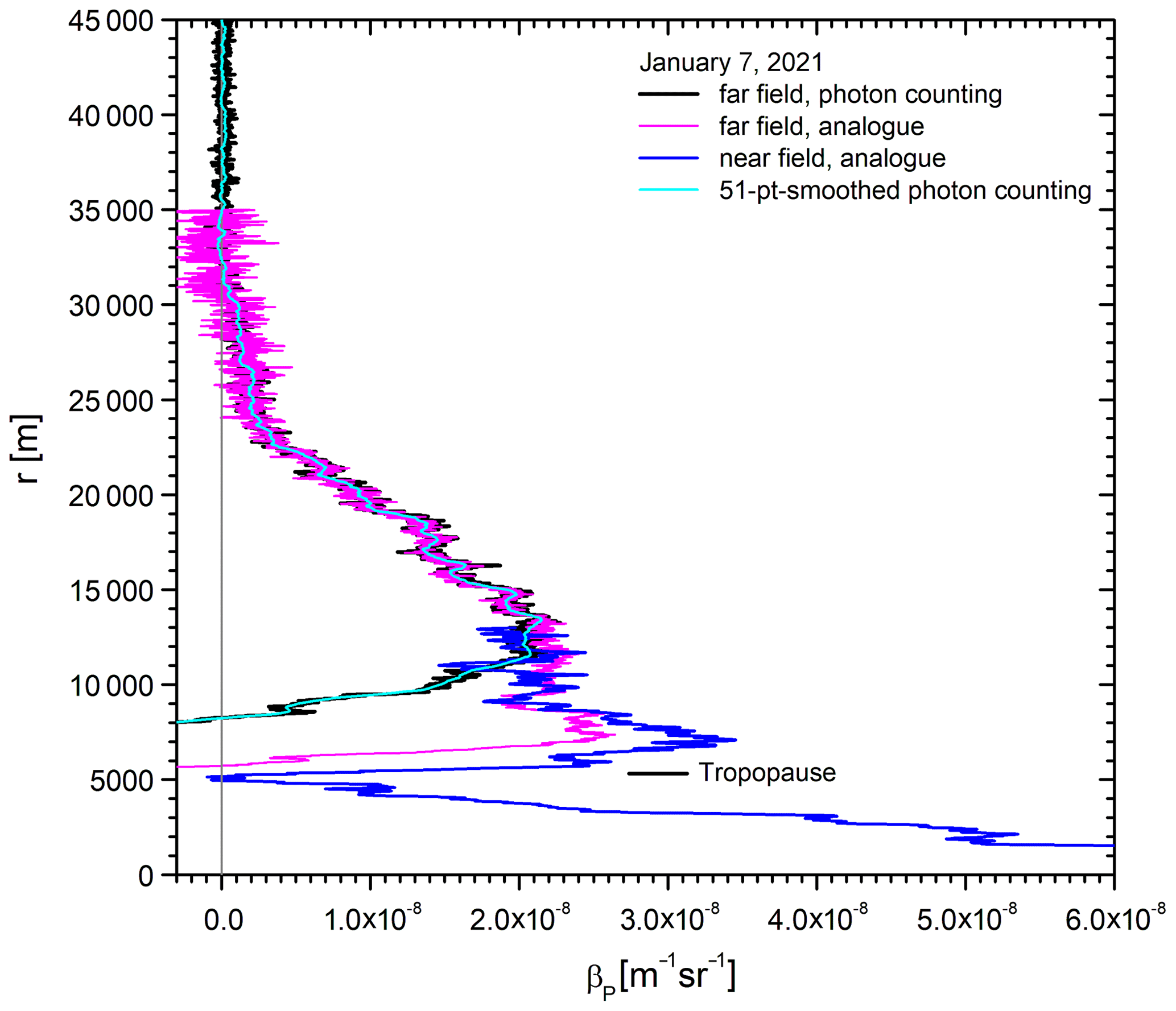
Figure 1 Backscatter coefficients from the Klett inversions of the data of the near- and far-field detection channels in the evening of 7 January 2021 (100 000 laser shots); the values are displayed with bin sizes of 7.5 m (old system: 75 m, same noise amplitude up to 40 km). The photon-counting values are smoothed with a ±25-bin sliding average that reveals the high far-field performance of the system. Please note the low wintertime Munich tropopause at r=5.3 km (h=8.0 km). r=0 m corresponds to 2675 m a.s.l. (laboratory at UFS). The aerosol below 5 km was advected from Ukraine and Türkiye.

The calibration of the backscatter coefficients is additionally controlled by the requirement that the backscatter coefficients must stay positive. Here, it is beneficial that layers without aerosol quite frequently occur in the upper troposphere.

The raw backscatter signals have been corrected for the light absorption by ozone in the stratosphere cross section for both the ruby wavelength (before 1990) and the wavelength of the frequency-doubled Nd:YAG laser (Brion et al., 1998; http://igaco-o3.fmi.fi/ACSO/cross_sections.html, last access: 8 February 2024). The values for λ_air=532.092 nm are almost temperature independent, ranging between 2.812 × 10⁻²⁵ m² (295 K) and 2.805 × 10⁻²⁵ m² (218 K). Climatological, seasonally varying ozone profiles have been taken, kindly provided by the nearby Meteorological Observatory Hohenpeißenberg (MOHp) of the German Weather Service (Deutscher Wetterdienst, DWD). Figure 2 shows that these corrections are by no means negligible in the altitude range of maximum ozone concentrations.

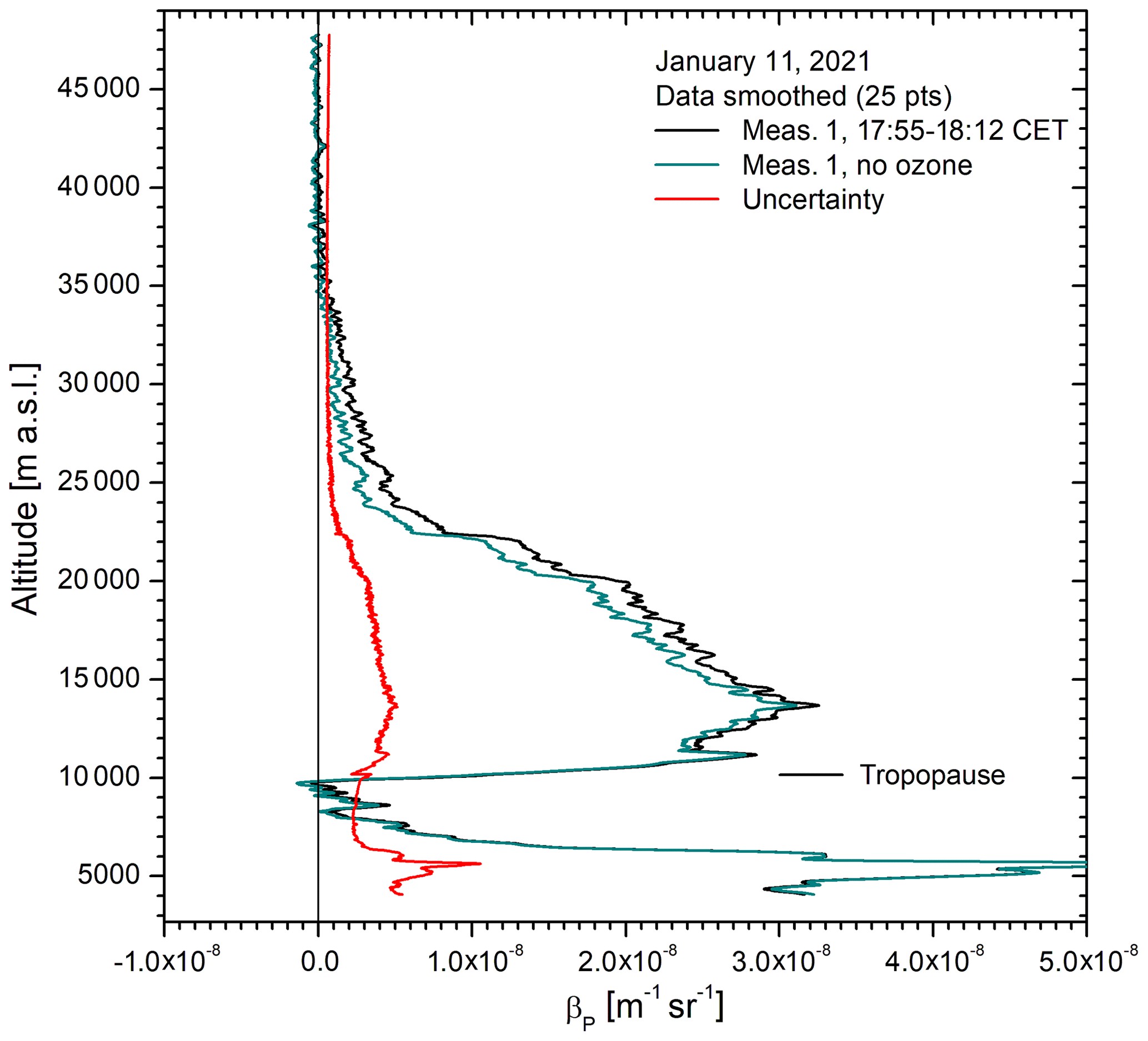
Figure 2 Comparison of the retrievals with (black curve) and without (blue curve) ozone correction (11 January 2021); the data were smoothed with a running arithmetic average over ±12 bins (±90 m).

An accurate determination of the tropopause altitude is crucial for the accurate calculation of the integrated backscatter coefficient in the stratosphere. It is normally extracted from the temperature data from the Munich radiosonde. Both the values for the World Meteorological Organization (WMO) criterion (WMO, 1986) and the temperature minimum are calculated. These values have been compared since 2012 with a number of ancillary data and modified if necessary (in rare cases). The validation and modification is derived from the ozone rise provided by the ozone differential-absorption lidar at IMK-IFU (Trickl et al., 2020a) whenever available, the drop of relative humidity in the sonde data and the upper edge of cirrus clouds (if present). Also the aerosol distribution in the tropopause region (e.g. cirrus clouds) has been used for refinements in unclear situations.

Because of the strong drop in signal the near-field raw data were smoothed with a linearly growing interval, using the Blackman-type numerical filter of Trickl et al. (2020a). At r=10 km the interval size reaches ±13 bins (±100 m), corresponding to a vertical resolution of roughly 40 m in the VDI definition and roughly 70 m as defined by the full width at half maximum of the response to a delta function (Trickl et al., 2020a).

A discussion of the uncertainties is given in Appendix B.

3 Results

3.1 Series of the integrated backscatter coefficient (1976–2023)

Figure 3 shows the updated version of the time series of the stratospheric integrated backscatter coefficient from 26 October 1976 to 11 October 2023. The integration starts at 1 km above the tropopause in order to reduce the influence of contributions of mixed tropospheric and stratospheric character. Since we cannot easily repeat the evaluation of the old data with all the microphysical details, we continued our tradition and converted the values from 532.24 nm to the ruby-laser wavelength of 694.3 nm (Jäger and Deshler, 2002, 2003).

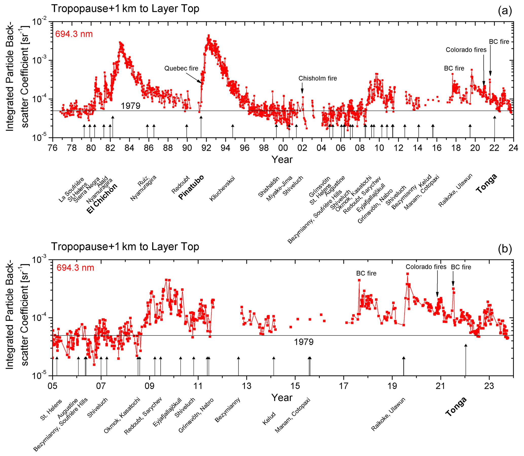
Figure 3 (a) Time series of the integrated stratospheric backscatter coefficient from the lidar measurements at Garmisch-Partenkirchen: the backscatter coefficients are integrated from 1 km above the tropopause to the upper end of the layer. (b) Section of (a) from 2005 to 2023.

In 2014 and 2015 the number of the measurements that could be stored in the computer strongly diminished due to data transfer issues, and the old lidar system was abandoned after a final measurement on 29 January 2016. Typical scattering ratios were about 1.05, i.e. rather low but higher than the very small pre-2006 background.

With the new system the routine sounding was resumed in 2017, after one test measurement on 17 March 2016. Until the end of the series several pronounced peaks are seen. The decay in 2022 led to values near the 1979 level, before a new phase of elevated aerosol prevented a return to a more pronounced background phase. In Table 1 we list some of the conditions of the measurements since 2017.

There is an obvious winter–summer modulation, visible in particular during the low-background period. This is mostly due to the changing tropopause. For example, the peak in January 2019 is mainly caused by tropopause altitudes of about 10 km, whereas they were of the order of 12 km in February. The seasonal cycle is somewhat obscured by occasional plumes just above the tropopause.

Between early 2014 and August 2017 there were just three major eruptions, all in the tropics (https://volcano.si.edu/, last access: 8 February 2024; more information on individual cases: https://volcano.si.edu/index.cfm, last access: 8 February 2024), and, thus, although they are not so important for observations at our latitude, these can contribute to the background with a delay of the order of half a year (Jäger, 2005). The Kelut plume (Java; volcanic explosivity index (VEI, Newhall and Self, 1982) = 4) reached as high as 17 km on 13 February 2014, and Manam (New Guinea) reached 19.8 km in a possibly brief explosion on 31 July 2015. The eruption of Cotopaxi is special since this volcano in Ecuador is the highest active volcano on the planet (5897 m). The material reached 17.9 km a.s.l. on 15 August 2015, not far from the tropical tropopause.

Between 2017 and February 2023 three eruptions may have influenced our series. In 2019 the volcanoes Raikoke (Kuril Islands) and Ulawun (New Guinea) spewed material into the stratosphere. On 15 January 2022 a particularly explosive eruption was reported on the Tonga Islands that reached about 58 km (Proud et al., 2022; Taha et al., 2022). Due to its occurrence in the Southern Hemisphere related particles were detected above Garmisch-Partenkirchen not before October, except for a single, accidental observation on 29 June 2022.

The pronounced peaks of the integrated backscatter coefficient registered with the new system since 2017 will be discussed in the following. Most importantly, in addition to the volcanic eruptions, a number of exceptionally violent fires led to significant rises in stratospheric aerosol. These fire events make this period particularly interesting, with peak backscatter coefficients and peak altitudes unprecedented for smoke in our series. In contrast to earlier years a much better analysis of the sources of stratospheric aerosol has become possible by a combination of extended transport modelling and satellite data.

3.2 Sudden increase in the occurrence of fire plumes deeply penetrating into the stratosphere

Until July 2017 volcanic eruptions were the main source of stratospheric aerosol detected above our site. An exception was the remarkable aerosol loading following a fire in Quebec in June 1991 just before the arrival of the Pinatubo plume (Fig. 3) that reached roughly 17 km a.s.l. above Garmisch-Partenkirchen (Carnuth et al., 2002; Fromm et al., 2010). After the big Chisholm fire in 2001 the IMK-IFU lidar detected aerosol to more than 6 km above the tropopause (Fromm et al., 2008b, Fig. 3) for a short period of time. However, in the measurements in recent years penetration into the stratosphere to more than 20 km has been observed (Baars et al., 2019; Torres et al., 2020).

Although an increase in the occurrence of strong fires might be expected in a drier climate (Fig. 2 of Trickl et al., 2013), the sudden rise in the number of cases and their outstanding violence is rather surprising.

3.2.1 British Columbia fires, 2017

The first and particularly spectacular signature after resuming the measurements at UFS in 2017 was identified as the result of the pyroCbs in British Columbia (BC) on 11 and 12 August 2017 that acted like a volcanic eruption (Peterson et al., 2018; Fromm et al., 2021). In general, the BC fire season during that year lasted several months, starting on 6 July. The tropospheric smoke plumes were repeatedly detected with the 313 nm channel of our ozone DIAL.

Our first observation of the BC plume with the UFS aerosol lidar took place on 25 August (Fig. 4), after a 17 d period without measurements. The daytime measurements (08:00 to 12:00 CET) with analogue data acquisition, apart from a few smaller peaks, showed a giant aerosol spike as high as 16 to 17 km a.s.l. The 532 nm backscatter coefficients ranged between 1.3 × 10⁻⁶ and 1.9 × 10⁻⁶ m⁻¹ sr⁻¹, corresponding to scattering ratios (ratio (β_R+β_P)$/{\mathit{\beta }}_R$ of the backscatter coefficients, where R denotes Rayleigh and P denotes particle) between 7.2 and 10.3. This value is exceptionally high for the stratosphere. For comparison, the Pinatubo maximum scattering ratio above our site in early 1992 was about 10 at 21 km. As mentioned in the Introduction, even higher stratospheric aerosol loading caused by the BC fires was reported by Ansmann et al. (2018) farther to the north, a few days earlier.

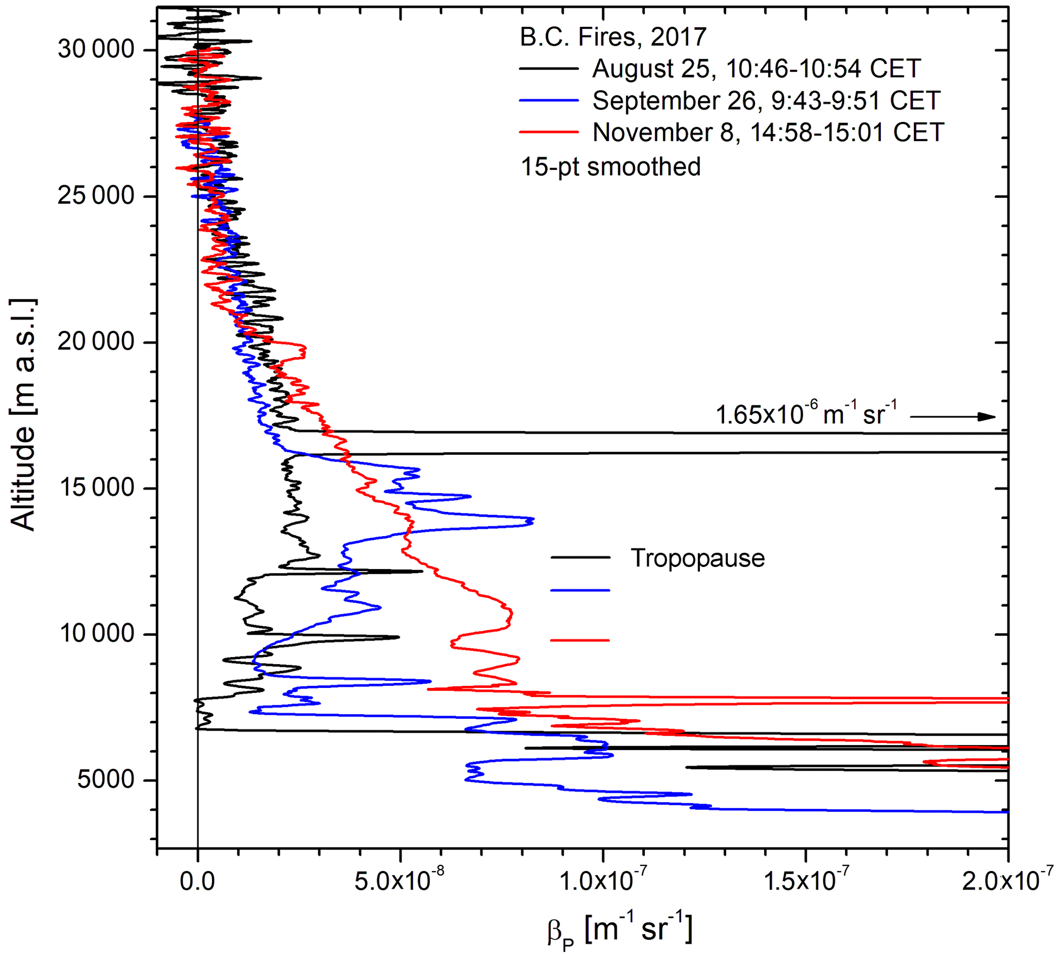
Figure 4 Three examples of 532 nm backscatter coefficients following the British Columbia (BC) fires in 2017; the data are slightly smoothed (sliding arithmetic average over ±7 bins) because of elevated noise due to analogue data acquisition, daytime conditions and just 20 000 laser shots. The corrected tropopause altitudes from the Munich radiosonde are marked in the colours of the corresponding backscatter coefficients.

The first burst of pyroCbs was reported by Fromm et al. (2021) for 12 August, at about 23:00 UTC; the last one was at about 06:45 UTC on the following day. Several times altitudes between 13 and 13.7 km were recorded by the Prince George radar.

Forward simulations with the HYSPLIT model (https://www.ready.noaa.gov/HYSPLIT_traj.php, last access: 8 February 2024; Draxler and Hess, 1998; Stein et al., 2015) initialized over the pyroCb area at that time showed passage above the Bavarian Alps on 20 and 22 August, in agreement with the observations by Ansmann et al. (2018) carried out before our first available measurement day (25 August; see Fig. 4). The forward trajectories do not show the rise to more than 16 km that is documented in Fig. 4. One cannot exclude a thermally induced rise (de Laat et al., 2012; Khaykin et al., 2018; Torres et al., 2020; Lestrelin et al., 2021; Ohneiser et al., 2023). The rise of the plume was verified by the “curtains” of the space lidar CALIOP (Cloud-Aerosol Lidar with Orthogonal Polarization, https://www-calipso.larc.nasa.gov/products/lidar/browse_images/production/, last access: 8 February 2024). Fromm et al. (2021) show a rise from 13 km over the Canadian western Arctic Ocean to more than 15 km over the northern part of the Hudson Bay. Lestrelin et al. (2021) followed the CALIOP images to Europe and found splitting of the plume into three parts and a rise to higher altitudes.

An approximate source–receptor relationship for 25 August was established by 315 h HYSPLIT ensemble backward trajectories (reanalysis mode), run for start altitudes above Garmisch-Partenkirchen between 15 300 and 17 200 m a.s.l. at intervals of 50 m. In this altitude range two principal branches are seen, one showing air passing over the United States (SB, southern branch) and one reaching the Canadian Arctic (northern branch, NB). Below 15 850 m the SB is almost exclusive. Above this altitude the NB becomes increasingly important.

In numerous transport studies (e.g. Trickl et al., 2013, 2015, 2020b) during the past decade we found that the HYSPLIT trajectories explain our observations better in the reanalysis mode (using National Center for Environmental Prediction reanalysis data). In this case and a case presented further below, the GDAS (Global Data Assimilation System) mode performs significantly better. In Fig. 5 we show the GDAS result for the altitude of 16 860 m, which yields the best proximity to the source region. The NB trajectories pass over the Arctic regions where the plume was located with the CALIOP images and almost perfectly hit the pyroCb source region within less than half a day of the most active period, on 12 August after 12:00 UTC. Given the uncertainty in trajectory calculations, the considerable spreading of the trajectories towards the west and the complex meteorology associated with the pyroCbs (Lestrelin et al., 2021), this result is highly satisfactory. Most importantly, we do not know about any other similarly strong aerosol source for that period.

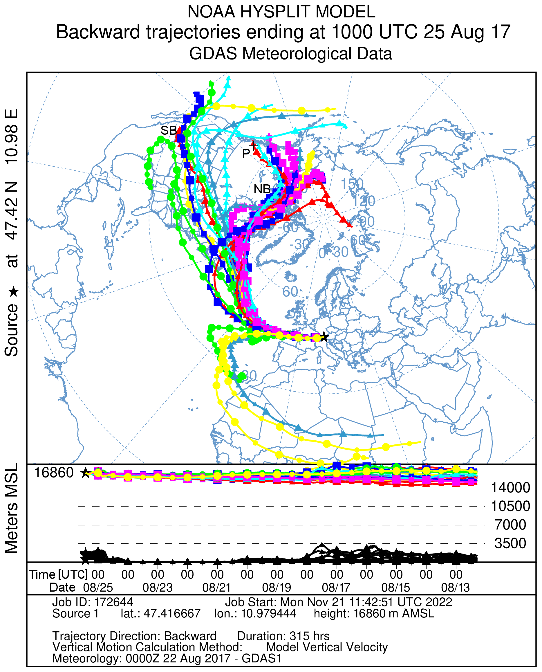
Figure 5 HYSPLIT 315 h backward ensemble trajectories initiated at 16 800 m a.s.l. above Garmisch-Partenkirchen (black asterisk). The cross labelled with P marks the approximate area of the pyroCbs. The two labels NB and SB mean northern branch and southern branch, respectively.

Fromm et al. (2021) show in their Figs. 3 and 9 the propagation of the densest part of the smoke close to the western end of the Great Slave Lake. In Fig. 5, the trajectories pass this area farther to the west, where less aerosol is depicted in that figure. This could explain why our peak backscatter coefficient is lower than that published by Ansmann et al. (2018). The backward trajectories slightly descend towards the source region, although not enough to exclude a thermal rise of the plume.

Between 25 August 2017 and the end of the year a total of 30 measurements were conducted. For the series image in Fig. 3 just one measurement per day was selected. Frequently daytime measurements took place. Until spring 2018 just analogue data acquisition was available that is fortunately highly linear after just minor correction (Sect. 2, Table 1).

On the following measurement day, 29 August (not shown), the big feature at 16.5 km from the first passage over central Europe had disappeared. In October another maximum of the integrated backscatter coefficients was reached, tentatively ascribed to a more dispersed phase of the plume with a higher probability of passing over southern Germany. The plume decayed considerably until December 2017 (for two autumn examples, see Fig. 4). The layer top rose from 17 km (25 August 2017) to more than 24 km in February 2018. This is slightly above the highest altitudes reported by Baars et al. (2019) in an overview for the EARLINET stations. The spiky structure of the backscatter profile gradually became smoother and disappeared in winter 2018 (not shown). The short decay of less than 1 year is typical of mid-latitude aerosol plumes in the stratosphere, as can be concluded from Fig. 3 (e.g. the eruption of Mt St Helens, 1980).

Apart from spreading to other latitudes stratospheric aerosol can be diminished by removal from the lowermost stratosphere in tropopause folds (e.g. Browell et al., 1987; Trickl et al., 2016). Also in autumn 2017 aerosol was found in stratospheric intrusion layers in our ozone soundings in the valley at IMK-IFU, this time during a period of aerosol from biomass instead of a volcanic plume in the lower stratosphere. Figure 6 shows three ozone and 313 nm aerosol profiles obtained with our ozone DIAL (Trickl et al., 2020a) on the morning of 2 October 2017, before the arrival of clouds (see aerosol spike at 9.45 km) around noon stopped the measurements. The descending intrusion layer, originating at more than 10 km over northern Canada 3 to 4 d earlier, is characterized by ozone mixing ratios up to almost 140 ppb, in agreement with the morning balloon-borne measurement at Hohenpeißenberg, 38 km to the north of UFS (Trickl et al., 2023). The minimum Hohenpeißenberg sonde RH is constantly 2 %, most likely a wet bias (Trickl et al., 2014, 2016). The aerosol backscatter coefficient in this layer reached 2 × 10⁻⁷ sr⁻¹ m⁻¹, which is moderate in comparison with other cases, in particular the record-setting 2.35 × 10⁻⁶ m⁻¹ sr⁻¹ observed on 7 September 2009 after the violent eruption of Sarychev (Trickl et al., 2020b). It is interesting to see that the elevated aerosol backscatter coefficients do not fill the entire intrusion layer, although the width scales similarly to that of elevated ozone. In the case described by Trickl et al. (2016) the aerosol maximized in the upper part of the intrusion.

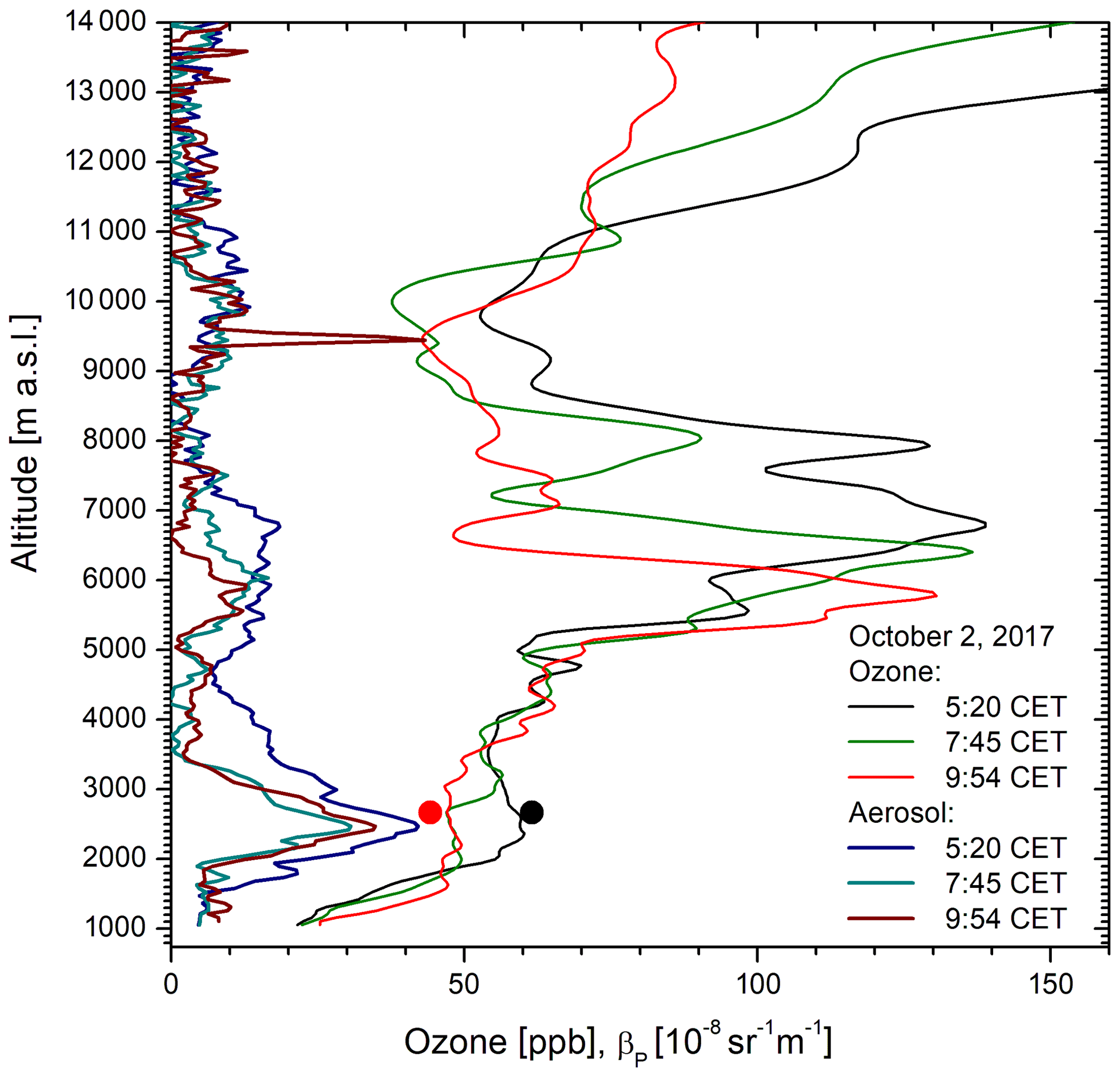
Figure 6 Ozone mixing ratios and 313 nm aerosol backscatter coefficients derived from measurements of the ozone DIAL at IMK-IFU on 2 October 2017, showing aerosol in a descending intrusion layer giving rise to a 313 nm aerosol backscatter coefficient of almost 2 × 10⁻⁷ m⁻¹ sr⁻¹ between roughly 5 and 7 km. The aerosol spike at 9.45 km could be a weak cirrus and mark the upper end of the troposphere. For comparison we also give the ozone mixing ratios measured at UFS at 05:30 and 10:00 CET (filled circles).

3.2.2 Siberia fires, 2019

Parallel to violent volcanic eruptions (Sect. 3.3) extreme and long-lasting wildfires in central and eastern Siberia were reported in the summer of 2019 (Johnson et al., 2021); Ohneiser et al. (2021) describe an Arctic field campaign in September and October 2019 with an advanced multi-wavelength polarization Raman lidar on board the German icebreaker RV Polarstern. The high lidar ratio indicated that the stratospheric aerosol observed at high latitudes was smoke. The air mass could be traced back to fires in Siberia. Also over central Europe they report for Leipzig and other lidar stations a contribution of these fires (see also Ansmann et al., 2021). In the absence of strong pyroconvection they conclude that the biomass-burning particles were limited to altitudes up to 13 km.

Without the planned high-spectral-resolution detection channel it is difficult for us to distinguish between the volcanic aerosol and the Siberian smoke. For more information on this period, see Sect. 3.3.

3.2.3 Colorado fires, 2020

The measurements in November and December 2020 were characterized by numerous spikes in the backscatter profiles in the upper troposphere and lower stratosphere (Fig. 7; the number of profiles is too low for a contour plot). The rather narrow structures on a broad background indicate sources just shortly backward in time. We ascribe these narrow aerosol layers to very late fires in Colorado. The narrow features harden the idea of rather fresh emissions. Indeed, HYSPLIT ensemble backward trajectories show an air-mass passage over that region. According to the MODIS (Moderate Resolution Imaging Spectroradiometer on board NASA's Aqua satellite) website the 2020 Colorado fire season has been devastating and record-breaking. The three largest fires in Colorado history all occurred during this year (https://modis.gsfc.nasa.gov//gallery/individual.php?db_date=2020-10-27, last access: 8 February 2024). The two most violent fires occurred in October 2020, very late in the year. The Cameron Peak Fire burned 844 km², and the East Troublesome Fire burned 779 km². The Cameron Peak Fire began in August and is the largest fire in state history; the nearby East Troublesome Fire pyroCb ignited on 14 October and explosively grew until 21 October (13.2 km) to capture the number-two title. At least 11 fires continued to be active in the state on 26 October.

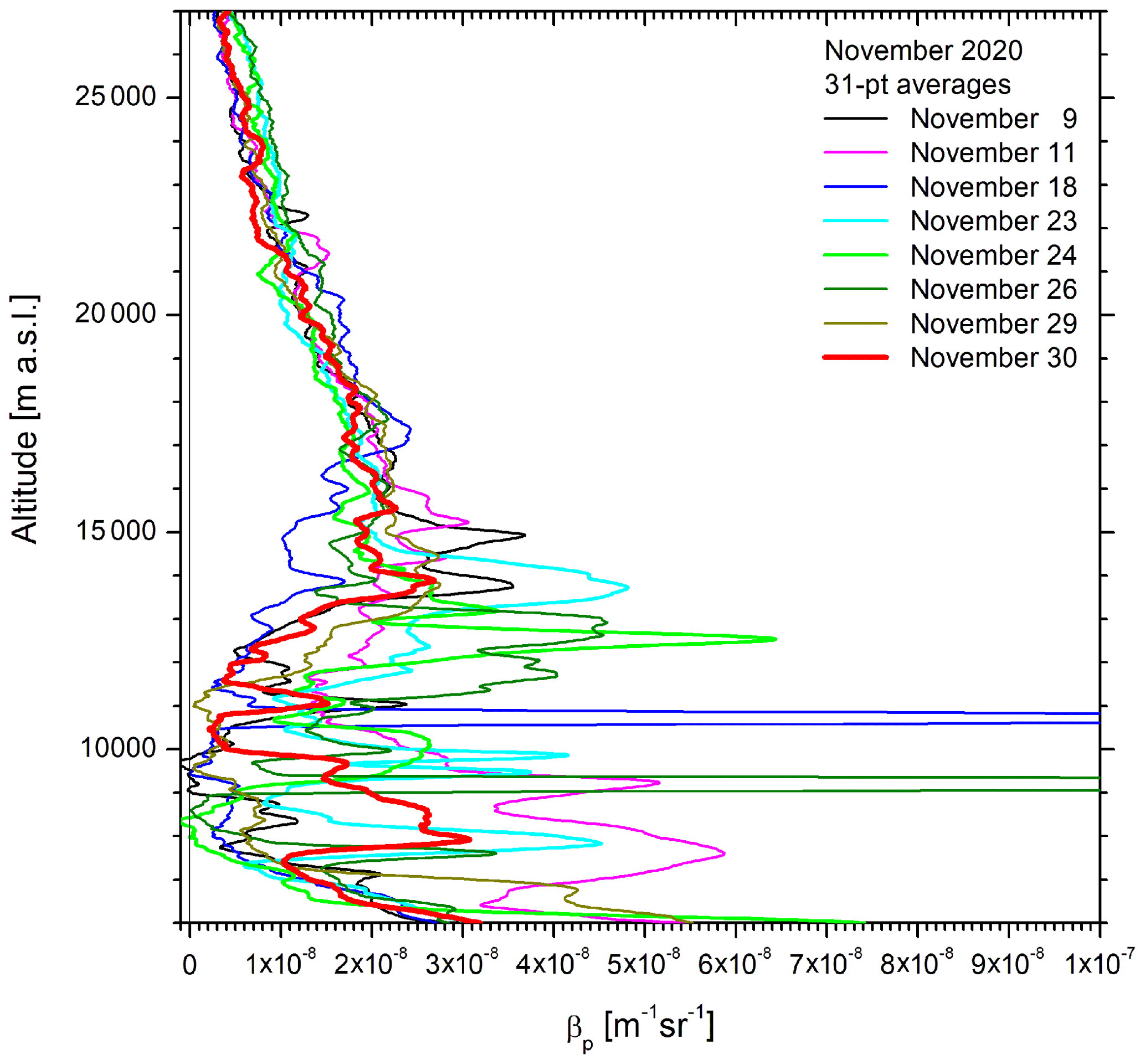
Figure 7 The 532 nm aerosol backscatter coefficients from the nighttime measurements in November 2020 showing the influence of the fires in Colorado; the two spikes leaving the scale are caused by cirrus clouds. The corrected tropopause altitudes of the Munich radiosonde are 12.65, 13.13, 12.57, 11.41, 11.40, 10.93, 12.34 and 13.06 km, respectively. See Fig. 1 for the situation after these plumes tapered off.

The plume was traceable around the world with satellite-based instruments such as MODIS, CALIOP and vertical soundings of the Micro-Pulse Lidar Network (MPLNET, https://mplnet.gsfc.nasa.gov/, last access: 8 February 2024). The particles from the 21 October East Troublesome Fire pyroCb in Colorado can be seen to flow over the Atlantic Ocean to reach Europe and North Africa on 25 October. Our first lidar measurement after the occurrence of the pyroCb on 28 October (not shown) shows small aerosol peaks above the smooth background between the tropopause and 14 km that could be a first indication of the fire plume. HYSPLIT ensemble backward trajectories initiated in this altitude range show zonal flow from Colorado to the Alps within just 3 d. The measurements during the following weeks (Fig. 7) show strongly varying structures and were not analysed in detail because of this complexity except for 9 November. The source–receptor relationship for the lidar measurements UFS on 9 November was hardened by the satellite and MPLNET measurements mentioned above, connected via HYSPLIT forward and backward trajectories. HYSPLIT ensemble trajectories initiated at and around 14.5 km a.s.l. above UFS on 9 November show a rather coherent near-zonal flow around the globe passing over North America twice within 315 h.

While the East Troublesome Fire pyroCb is a plausible source for these November stratospheric layers, we cannot rule out contributions from earlier pyroCbs in the USA. For instance, the Creek fire in California developed its own spectacular pyroCb on 3 September, injecting smoke upward of 16 km (Hu et al., 2022; Lareau et al., 2022). Late Californian contributions (26 October to 3 November) were found in the upper troposphere above the Mediterranean region (Michailidis et al., 2023; Mamouri et al., 2023).

3.2.4 Spectacular pyrocumulonimbus in British Columbia on 30 June 2021

The measurements on 11 and 21 July 2021 show pronounced stratospheric aerosol signatures that lead to clearly enhanced backscatter coefficients (Fig. 3). We discuss here just the particularly spectacular case of 11 July (Fig. 8). We observed enhanced aerosol structure in the upper troposphere and in the stratosphere up to about 19.5 km. This upper edge is absent in earlier measurements during this season. There are four pronounced spikes between 13 and 16 km. The big spike at 15.6 km with a remarkable backscatter coefficient of 7.07 × 10⁻⁷ m⁻¹ sr⁻¹ is very thin, which indicates an event just a few days backward in time. The maximum value is more than half that obtained for the 2017 fires (see above). The 532.2 nm integrated backscatter coefficient rose to 6.59 × 10⁻⁴ sr⁻¹ (3.16 × 10⁻⁴ sr⁻¹ at 694.3 nm, Fig. 3).

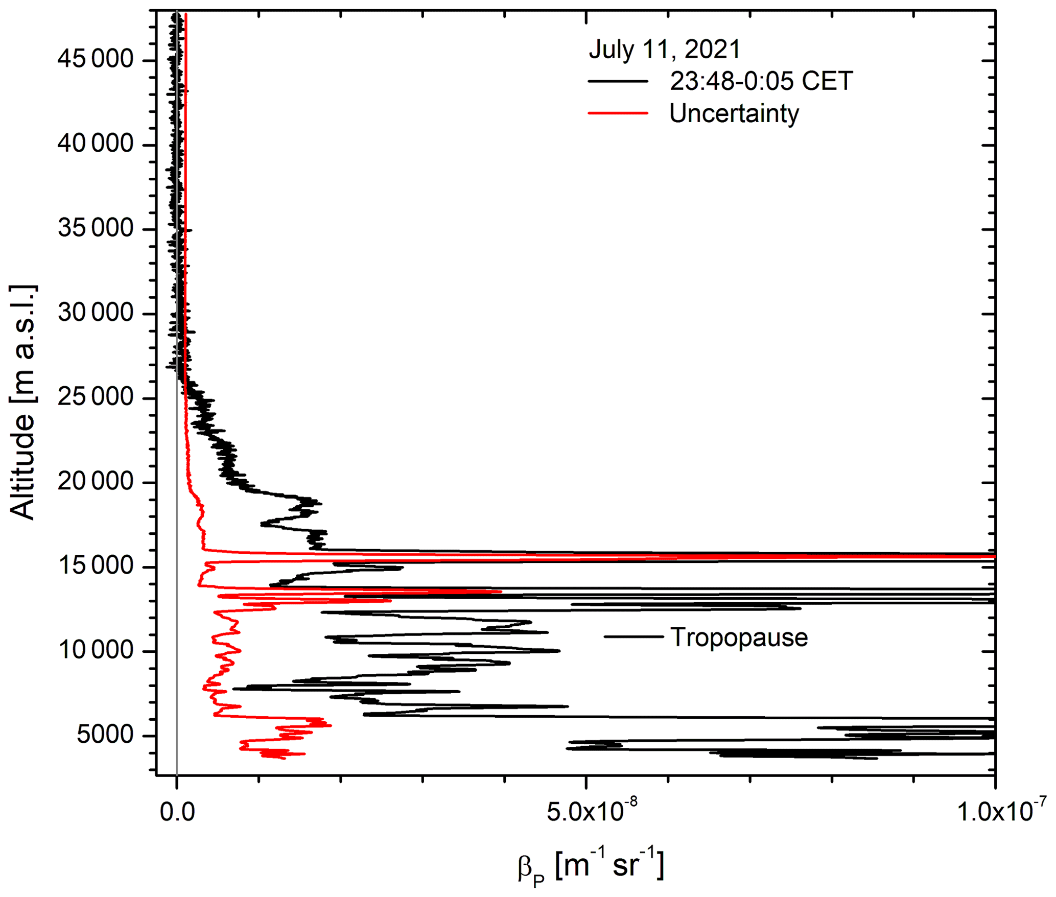
Figure 8 The 532 nm aerosol backscatter coefficients on 11 July 2021; the two maximum values are 2.63 × 10⁻⁷ m⁻¹ sr⁻¹ at 13.5 km and 7.07 × 10⁻⁷ m⁻¹ sr⁻¹ at 15.6 km. The relative uncertainty at 15.6 km is estimated to be 18 %.

We relate this observation to high pyroCb activity on 30 June, again in British Columbia. There are reports on record-setting temperatures of more than 45 ^∘C in that region, a drought, numerous lightning strikes under dry conditions and huge fires. An article from The Washington Post on 1 July 2021 (https://washingtonpost.com/weather/2021/07/01/wildfires-british-columbia-lytton-heat/, last access: 8 February 2024) gives a good overview, citing several scientists, and includes a picture with an impressive, very thick smoke “mushroom” clearly reaching into the stratosphere. The pyroCb burst most likely responsible for our observation occurred at 51.0^∘ N, 120.8^∘ W, at times between 19:00 UTC on 30 June and after UTC midnight. The Seattle radar yields a maximum altitude of 17.3 km at 02:12 UTC. This altitude exceeds that of the largest peak in Fig. 7.

Unfortunately, we could not find a suitable “aerosol curtain” in the images derived from the measurements of CALIOP visualizing the fire plume right after the event. However, we inspected numerous graphics of the Multi-angle Imaging SpectroRadiometer (MISR, https://misr.jpl.nasa.gov/, last access: 8 February 2024) and the Micro-Pulse Lidar Network (https://mplnet.gsfc.nasa.gov, last access: 8 February 2024) to establish the path of the smoke.

The interpretation was hardened by running numerous HYSPLIT 315 h forward and backward trajectories for different start altitudes with the GDAS option. As in the case of the 2017 fires there is no homogeneous flow pattern, with the path of the trajectories strongly varying with altitude. In Fig. 9 we show ensemble trajectories initiated at 15.6 km a.s.l. and 23:00 UTC (24:00 CET) above IMK-IFU; the position of the largest aerosol spike in Fig. 8 and start positions varied by one grid point. As mentioned there is a strong sensitivity on start time and position. One trajectory bundle leads backward towards British Columbia, and three trajectories from this bundle end not far from the position of the main pyroCb 261 h backward in time (1 July, 02:00 UTC, almost within the pyroCb period mentioned above). The trajectory results for the aerosol peaks between 12.3 and 13.8 km are less perfect. Again, this result is highly satisfactory given the complex meteorology of a pyroCb including radiation-induced lofting (see 2017 case).

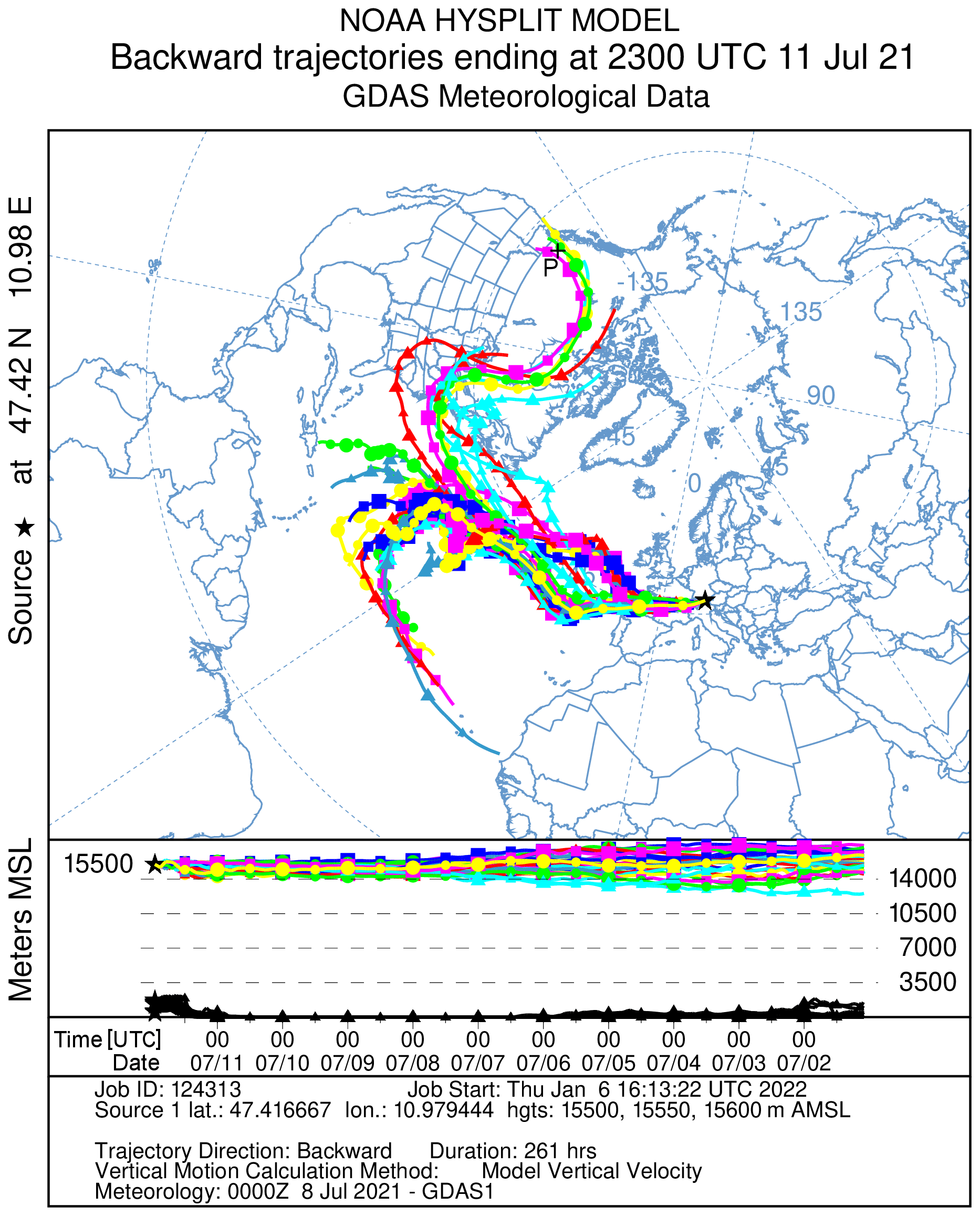
Figure 9 HYSPLIT ensemble backward trajectories initiated at 15.55 km ± 0.05 km a.s.l. above UFS (Garmisch-Partenkirchen) on 11 July 2021 (23:00 UTC). The duration of the trajectories is 261 h (see text); the most likely pyroCb position at 51.0^∘ N, 120.8^∘ W is marked with a black cross (labelled with P).

The trajectory results provide evidence that the main burst of the plume directly passed over our site during the first round around the globe. This explains the very sharp structure of the spikes.

3.3 Volcanic eruptions in June 2019 and January 2022

3.3.1 Eruptions in 2019

In June 2019 there was the interesting case of an almost co-incident volcanic eruption in the tropics and in the mid-latitudes. According to information from the Global Volcanism Program (GVP) of the Smithsonian Institution (https://volcano.si.edu/index.cfm, last access: 8 February 2024) the Raikoke volcano on the Kuril Islands (48.292^∘ N, 153.23^∘ E; summit 558 m a.s.l.) erupted on 21 June 2019. Cameron et al. (2021) reported strong SO₂ after the Raikoke eruption at 24 km, tapering off within 4 months. Boone et al. (2022) and Knepp et al. (2022) discuss the satellite observations of SO₂ and sulfate, with the latter having been observable until the following spring, obviously at a different cut-off level.

Subsequently, Ulawun (New Guinea, 5.05^∘ S, 151.33^∘ E; summit: 2334 m a.s.l.) violently erupted on 26 June 2019. The maximum altitude reached was 19.2 km which should be within the tropical stratosphere. A plume component at 16.8 km is reported to having drifted north-eastward to north-westward. Both eruptions were studied by Kloss et al. (2021).

Our first observation of two small aerosol peaks just above the tropopause that could be related to the Raikoke plume took place on 19 July 2019. The signal could not be inverted because tropospheric clouds strongly attenuated the signal. From 23 July to 1 September a number of spikes appeared between the tropopause and 19.5 km, i.e. less than the maximum plume height reported by Cameron et al. (2021). The spiky distribution gradually changed to a less structured hump (Fig. 10). The maximum backscatter coefficient above the respective tropopause was 4.18 × 10⁻⁷ m⁻¹ sr⁻¹ on 23 July (the unidentified spike at 12.8 km with 7.53 × 10⁻⁷ m⁻¹ sr⁻¹ could be due to a cirrus). This is quite high for stratospheric aerosol. The maximum integrated backscatter coefficient was calculated for 22 August (5.4 × 10⁻⁴ m⁻¹ sr⁻¹, 693.4 nm). It exceeded those for the eruptions of Mt St Helens and Alaid in the early 1980s and is the third highest in our series, following the maxima for Pinatubo and El Chichón. The temporary minimum of the integrated backscatter coefficient in September 2019 is caused by very high tropopause levels up to 15 km. The structured contributions after the Raikoke eruption gradually tapered off until January 2020, reaching a maximum altitude of 22 km. They were followed by a smooth hump with elevated aerosol (up to 5 × 10⁻⁸ m⁻¹ sr⁻¹) ending between 20 and 21 km.

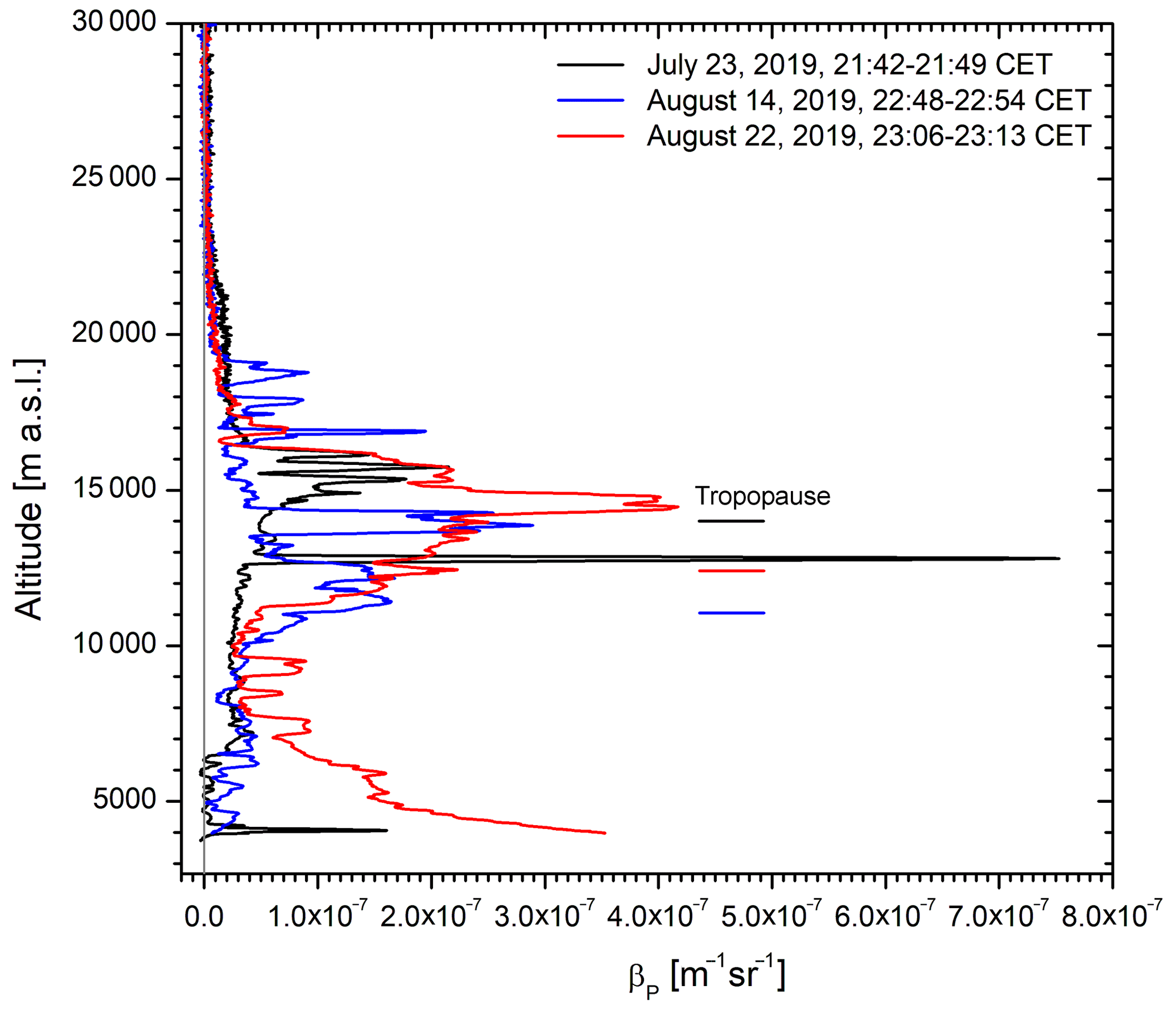
Figure 10 High 532 nm aerosol backscatter coefficients following the Raikoke volcanic eruption in June 2019; the tropopause levels are 13.89, 11.06 and 12.40 km, respectively. We tend to assume that the spike at 12.8 km on 23 July was caused by a cirrus cloud because it is located below the tropopause. However, the Munich relative humidity at that altitude was less than 30 %. The tropopause altitudes are marked in the colours of the respective backscatter coefficients.

As mentioned in Sect. 3.2 Ansmann et al. (2021) and Ohneiser et al. (2021) emphasize the additional influence of Siberian fires during that summer. We defer to the view in that paper, derived from differences in the retrieved extinction-to-backscatter ratios. Ohneiser et al. (2021) conclude that the volcanic portion of the aerosol is mostly that at higher altitudes.

It is interesting that the decay of the integrated stratospheric backscatter coefficient is slower than after most mid- and higher-latitude volcanic eruptions (Fig. 3). We speculate that this could be due to the larger area of these strong fires in comparison with a volcanic point source and longer-lasting burning, leading to wider horizontal spread of the particles. Alternatively, Khaykin et al. (2022a) describe a long-lasting anticyclone that circumnavigated the globe three times and ascended diabatically to 27 km altitude through radiative heating of volcanic ash in the plume.

There is some indication that we are able to distinguish between contributions from both 2019 eruptions in our data. This distinction is based on a delayed arrival of what we could ascribe to the tropical component (see Jäger, 2005) for the eruptions of El Chichón and Pinatubo. On 20 December 2019 a sudden rise in the upper boundary of the stratospheric aerosol to clearly beyond 30 km started. Such a rise would require a Brewer–Dobson-type lifting of the tropical air mass.

In Fig. 11 we give a few examples of smoothed scattering ratios from the times before, during and after that period of enhanced aerosol. Up to 35 km the uncertainty of these values stays within ±0.03. The noise level above 35 km becomes rather high (up to ±0.1) because the scattering ratio implies a division by the strongly decreasing molecular backscatter coefficient. It is, therefore, difficult to determine precisely the cut-off altitude if it lies between 35 and 40 km. The scattering ratio was almost constant up to the upper boundary and typically ranged between 1.04 and 1.10. This indicates a rather homogeneous aerosol distribution in agreement with the idea of long transport times.

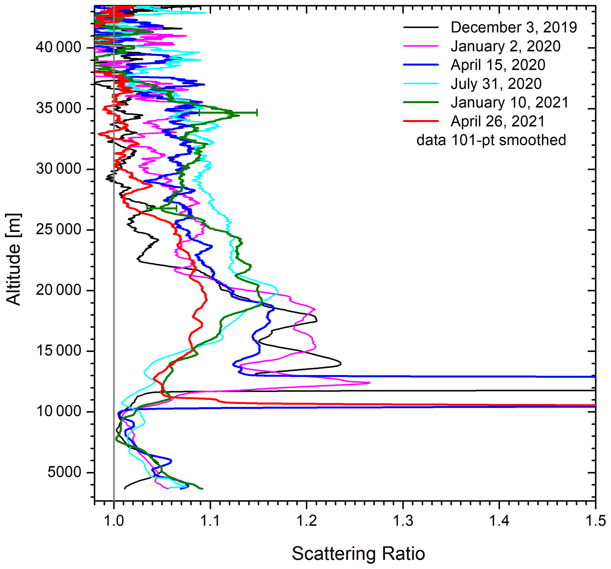
Figure 11 The 532 nm scattering ratios smoothed by gliding ±50-bin averages for selected measurements in 2019, 2020 and 2021; starting in January 2021 the aerosol layer expanded to more than 28 km a.s.l., possibly caused by northward propagation of the plume from the tropical eruption of Ulawun in the Brewer–Dobson circulation. The uncertainty in the values strongly grows above 35 km because the relative noise in the data starts to exceed the size of the aerosol features.

Figure 12 shows the time series of the principal aerosol upper boundaries determined from the retrieved profiles of the backscatter coefficients. The boundaries are crude estimates and (if discernible) correspond to altitudes where the aerosol disappears or reaches a bottom line. On 26 April 2021 the layer extension to beyond 30 km completely disappeared (Fig. 13). Apart from very small occasional peaks this remained unchanged until the end of the measurements included in this paper.

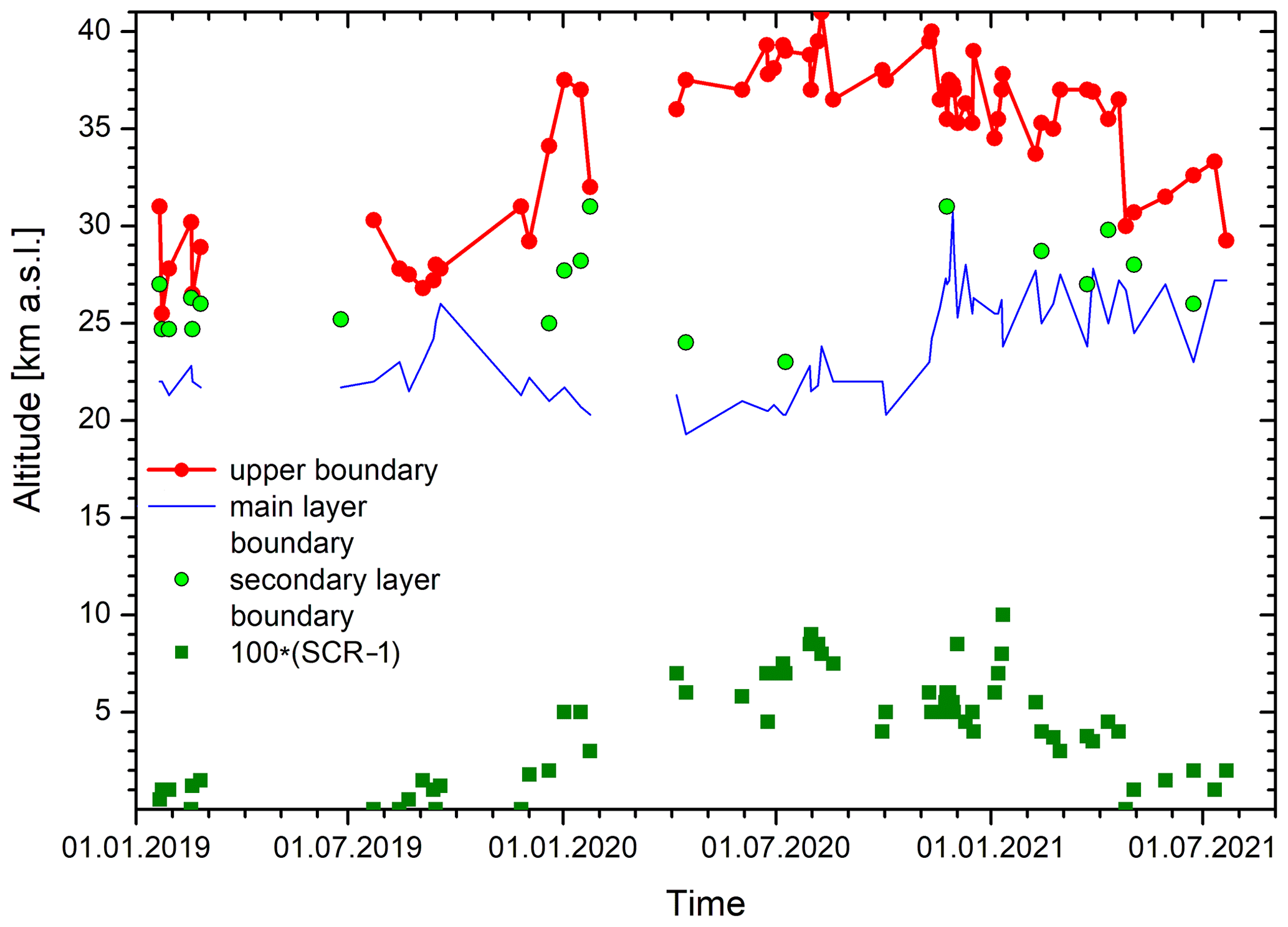
Figure 12 Upper boundaries of the top aerosol layers after the two big volcanic eruptions in July 2019: “main layer” (blue) means more a pronounced aerosol feature already present before that period. We speculate that the rise in the upper part of the top boundary (red) was caused by northward propagation of the tropical eruption of Ulawun in the Brewer–Dobson circulation. The average scattering ratio (SCR) above 30 km is slightly elevated. The date format used in this figure is day.month.year.

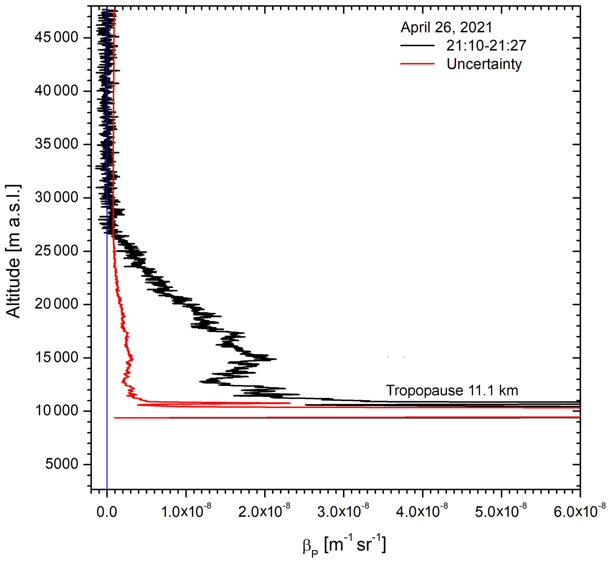
Figure 13 The 532 nm aerosol backscatter coefficients for 26 April 2021: there are no longer aerosol contributions above 30 km. The strong cirrus signal did not allow for reasonable data evaluation within the troposphere.

These observations are further discussed in Sect. 4, in comparison with the Pinatubo results (Jäger, 2005).

3.3.2 Hunga Tonga, 2022

The most violent volcanic eruption in recent history occurred on 15 January 2022, lasting just 11 h. The Hunga Tonga–Hunga Ha'apai submarine volcano (20.55^∘ S, 175.4^∘ W) injected material, including huge amounts of steam (Schoeberl et al., 2022; Xu et al., 2022; Vömel et al., 2022), into the stratosphere up to as high as 58 km, far beyond the 40 km reached by the Pinatubo eruption (Proud et al., 2022; Taha et al., 2022). The bulk of the plume circulated the globe in the Southern Hemisphere at altitudes between 20 and 30 km. Most of the poleward expansion occurred in the Southern Hemisphere. However, some material also reached the Arctic. In the tropics maxima between 20 and 45 ppm of water vapour were detected between 25 and 26 km by sonde ascents (Vömel et al., 2022).

Also at high latitudes observations of the plume were made. Taha et al. (2022) traced an aerosol layer observed at 83^∘ N, 29^∘ E and 21 km on 4 April 2022 back to the Hunga Tonga cloud. Khaykin et al. (2022b) verified northward transport to 80^∘ N within 3 to 4 months by using satellite and lidar measurements. The altitude range was 20 to 25 km (see also Mishra et al., 2022).

The only measurement of the UFS aerosol lidar showing a conspicuous feature in spring and summer 2022 was made on 29 June (Fig. 14). A small aerosol peak, not seen in other measurements during that period, occurred at 22.75 km. This is between the altitudes in the observations of the Tonga plume at Haute Provence (southern France) and Kühlungsborn (northern Germany) as presented by Khaykin et al. (2022b).

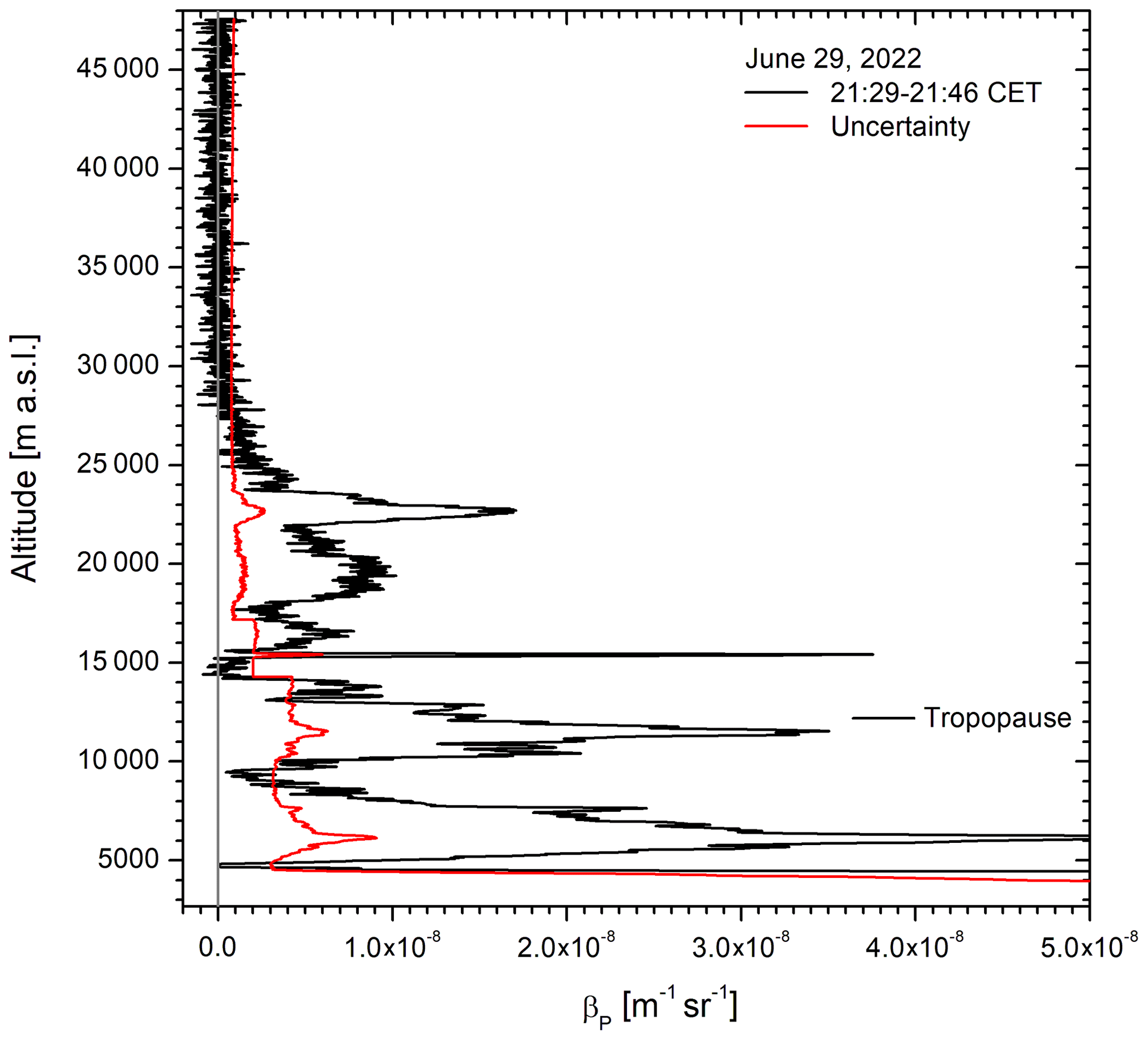
Figure 14 The 532 nm backscatter coefficients for the nighttime measurement on 29 June 2022: the peak at 22.75 km is attributed to aerosol from the Hunga Tonga eruption on 16 January 2022 (see text). Please note the rather low backscatter coefficients between 15 and 20 km that indicate the progress of aerosol removal from the stratosphere above our region after the recent events (see Fig. 12).

In order to identify the advection path for the peak in Fig. 14 we calculated HYSPLIT 315 h backward trajectories for re-analysis data and in ensemble mode (Fig. 15). The air mass arrived from the east and passed over China on 17 June. Figure 16 shows aerosol curtains of the Ozone Mapping and Profiler Suite (OMPS) limb sounder for the start and end times of the trajectories. On 29 June the orbits closest to Garmisch-Partenkirchen (UFS) a feature with elevated aerosol extinction ratio around 22.5 km conforms to the lidar observation. This is just indicative of the presence of Tonga particles. However, the Asian orbit on 17 June (lower panel) reveals a direct connection to the Tonga plume depicted in a dark colour at the same altitude across the Equator.

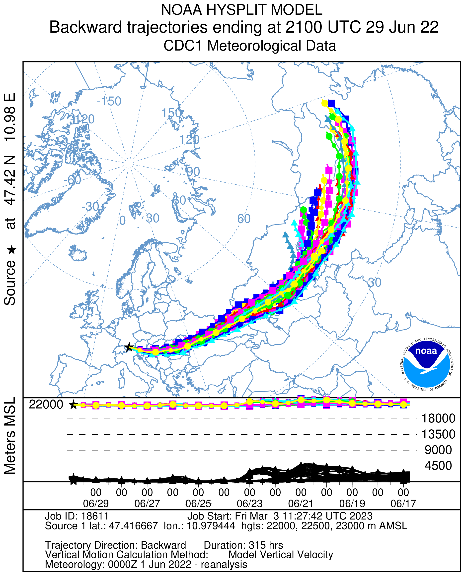
Figure 15 HYSPLIT 315 h ensemble backward trajectories initiated above UFS on 29 June 2022 at 22:00 CET.

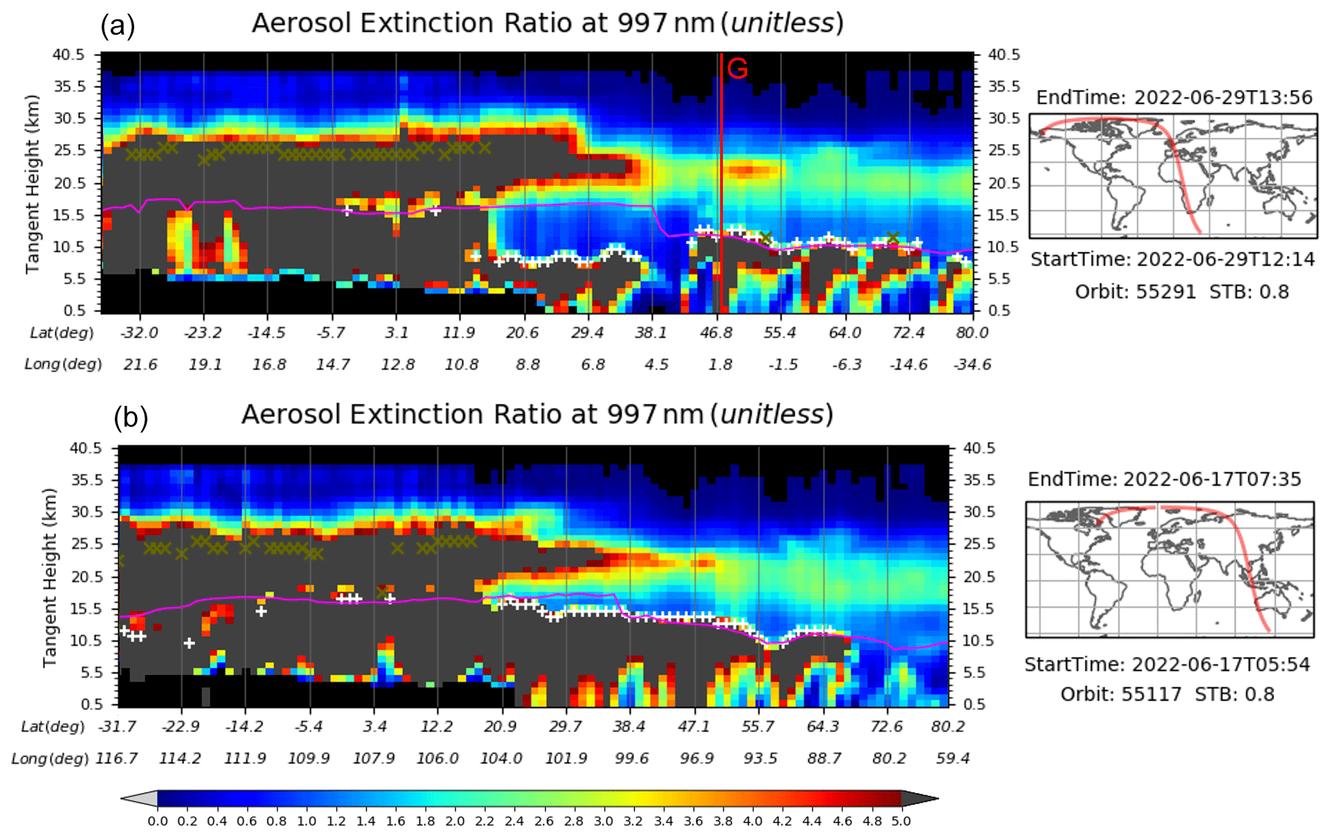
Figure 16 OMPS vertical distribution of the 997 nm aerosol extinction ratio for orbits (a) closest to UFS on 29 June and (b) over East Asia on 17 June as indicated in Fig. 15; the vertical red line labelled with G marks the latitude of Garmisch-Partenkirchen. The panels to the right show the corresponding orbits of the satellite (red lines).

No peak around this altitude was seen again before the measurement on 5 October. Starting in October elevated aerosol was found around and below 20 and below 25 km. In Fig. 17 we show the scattering ratios for four selected measurements from the period between October 2022 and February 2023. The relative importance varies with time; a minimum was found for the end of December and January. This (and the changing tropopause) explains the strong variation in the integrated backscatter coefficients in Fig. 3.

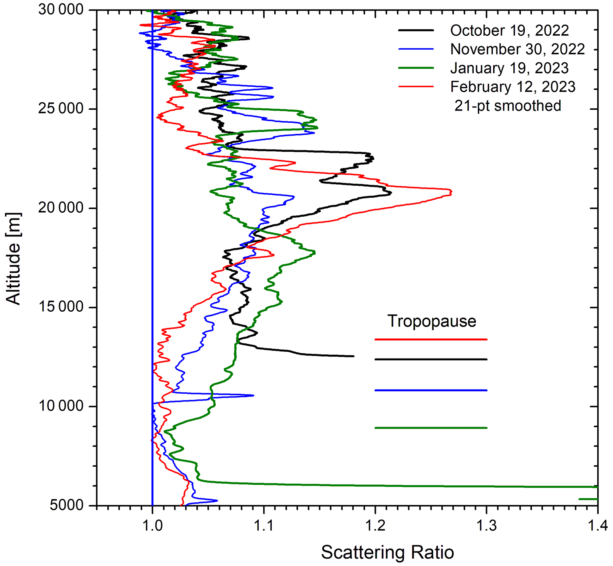
Figure 17 Four selected profiles of aerosol scattering ratios between October 2022 and February 2023; the data are smoothed with ±10-bin gliding arithmetic averages. The tropopause altitudes are marked in the colours of the respective scattering ratios.

On 19 October for the first time a particularly pronounced peak structure was retrieved (Fig. 17). This is confirmed by an OMPS aerosol curtain (Fig. 18). We prefer to display the extinction coefficients instead of the extinction ratio for greater clarity. This reduces the sensitivity for the aerosol structures in the Northern Hemisphere. As in Fig. 16 the stratospheric aerosol maximizes in the tropics and the Southern Hemisphere, as one would expect from the position of the Tonga archipelago. The x-shaped crosses at 25 km indicate a separate aerosol layer, slightly above the lidar peak.

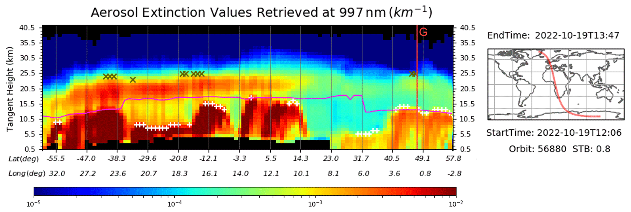
Figure 18 Section of an OMPS curtain of the aerosol extinction coefficient along an orbit passing not far from Garmisch-Partenkirchen depicted in the right panel (19 October 2022); the elevated stratospheric aerosol caused by the Tonga eruption is located between roughly 56^∘ S and 15^∘ N, with dark crosses marking pronounced aerosol layers. Slightly elevated aerosol is seen around 47^∘ N, where also a few dark crosses are visible at 25 km. The violet line corresponds to the tropopause. The vertical red line visualizes the latitude of Garmisch-Partenkirchen (G).

Also during the following months the lidar aerosol maxima are located below the OMPS crosses. Around the latitude of UFS (47.5^∘ N) no cross exists anyway, in agreement with lower structures in the UFS backscatter coefficients. Figure 19 shows the situation for 12 February 2023: the OMPS aerosol below 20 km had grown considerably, which is confirmed by the pronounced peak for 12 February in Fig. 19. The corresponding OMPS extinction ratio (not shown) exceeds the colour scale in that image.

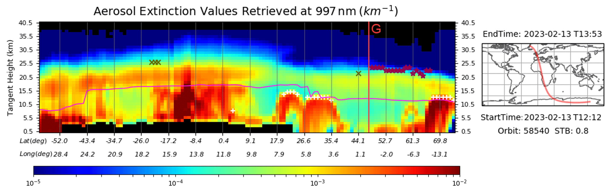
Figure 19 Section of an OMPS curtain of the aerosol extinction coefficient along an orbit passing to the west of Garmisch-Partenkirchen depicted in the right panel (13 February 2023), with dark crosses marking pronounced aerosol layers and red asterisks marking polar stratospheric clouds as determined by the OMPS algorithm. Slightly elevated aerosol is seen around 47^∘ N, where also a few dark crosses are visible at 25 km. The violet line corresponds to the tropopause. The vertical red line visualizes the latitude of Garmisch-Partenkirchen (G).

Motivated by the results of Vömel et al. (2022) we inspected the relative humidity (RH) distribution in the Munich radiosonde data. Normally, the RH values of the RS41 sonde launched by DWD decrease to 1 % within a few kilometres above the tropopause, with 1 % mostly being the lowest value listed. Starting in October 2022 RH ≥2 % became more and more frequent. By February 2023, the maximum RH ranged between 3 % and 5 %, with 12 % on 13 February. The range of particularly elevated humidity was located clearly above the aerosol maximum.

The elevated RH values are strongly indicative of the Tonga plume. However, the RH maxima are located above the aerosol maxima. However, Khaykin et al. (2022b) demonstrated that the humidity layers may differ in altitude from layers with depolarizing particles.

Measurements with our Raman lidar (Klanner et al., 2021) in February 2023 indicate an increase in the water-vapour mixing ratio above 17 to 20 km, with an indication of further rise towards higher altitudes. However, the laser power was low, which resulted in strongly enhanced uncertainty starting in this altitude range, and we prefer not to emphasize these findings.

The stratospheric aerosol quickly diminished in summer 2023. The upper boundary in October 2023 was roughly 26 km. This changed on 11 November, when we surprisingly observed some aerosol structure up to 34 km. The backscatter coefficients at the high altitudes were not strong, which seems to exclude a fresh powerful eruption. Thus, we speculate on a return of the Hunga Tonga plume. Given the resubmission deadline, we did not analyse this further.

4 Discussion and conclusions

With the new lidar at UFS the long-term Garmisch-Partenkirchen stratospheric aerosol series has been continued since March 2016. The signal-to-noise ratio of the system has greatly improved, allowing for a better performance for 7.5 m vertical bins than previously with 75 m bins. The data evaluation, based on a Klett algorithm, now starts at r=45 km (h=47.7 km), but this could be extended even to larger distances. The limit is given by the NCEP pressure and temperature data used for the calibration of the aerosol backscatter coefficients that end before 55 km a.s.l.

The integrated aerosol backscatter coefficients (Fig. 3) are dominated by the contributions from the first kilometres above the tropopause. Here, particles from moderate mid- and high-latitude volcanic eruptions, pyroCbs, desert dust (Trickl et al., 2013), and aircraft emissions cause a pronounced variability, sometimes featuring a spiky structure. These aerosols are removed at short to moderate timescales by stratosphere-to-tropopause transport (e.g. tropopause folding, Fig. 6; Stohl et al., 2003) and dilution. Above 25 km the aerosol contributions in our data mostly disappear within less than 1.5 years. After the removal at low and high altitudes the maximum scattering ratio is typically observed around 20 km.

Vernier et al. (“Do lidar systems have enough sensitivity to detect annual cycling in stratospheric aerosol scattering ratio?”, personal communication, 2013) concluded from satellite-based measurements that a calibration of an aerosol lidar with stratospheric capability must take place beyond 40 km. This is definitely true for tropical stations where the aerosol is likely to extend to higher altitudes than in the mid-latitudes. Indeed, the Mauna Loa lidar observations quite often show aerosol at 37 to 38 km (John Barnes, personal communication, 2021). However, for our mid-latitude station we normally find upper boundaries of the aerosol between 25 and 30 km. In any case, given the performance of the new system, we are now prepared for periods with minor amounts of aerosol reaching to at least 35 km as found during a 1-year period in recent years (see below).

The background phase of 1999 to 2008 was rather special. The particularly low integrated backscatter coefficients during that period yielded integrated backscatter coefficients down to about 40 % of the 1979 average background (horizontal line in Fig. 3) that were never reached again later on. Most likely, the 1979 background did not represent a minimum during that period because of the tropical Fuego eruption in 1974. The very remarkable aerosol depletion on some measurement days calls for more elaborate analysis of the reasons, such as troposphere-to-stratosphere transport (TST).

Indeed, TST was observed by us in a few cases in recent years and resulted in low aerosol up to a few kilometres above the tropopause (not presented here). For example, the occurrence of TST has been associated with upward transport in warm conveyor belts (WCBs; e.g. Stohl and Trickl, 1999; Trickl et al., 2003). Stohl (2001), Wernli and Bourqui (2002), and Madonna et al. (2014) estimated that overshoots of WCB air into the stratosphere can reach 10 % or more. In addition, frequent vertical exchange between the troposphere and the stratosphere occurs along the subtropical jet stream (Sprenger et al., 2003; Trickl et al., 2011).

Aerosol sources were not completely absent during the low-background period. In particular there were strong eruptions in the tropics (Vernier et al., 2011a), but obviously they did not significantly influence our observations. Most relevant for our station are mid-latitude eruptions to at least 10 km (Table 1 of Trickl et al., 2013). However, mid-latitude events with layer tops of 12 km and higher did not occur before 2006.

After the background phase there were two periods with clearly enhanced stratospheric loading, 2008 to 2012 and since 2017, which is the most spectacular phase since the Pinatubo eruption. In 2020 and early 2021 some aerosol extended to more than 35 km, tentatively ascribed to the tropical Ulawun eruption. This would be supported by Stenchikov et al. (2021), who report a maximum altitude of 35 km on the basis of model calculations and SAGE data (cited by these authors as Thomason and Peter, 2006), after a rise from initial 17–26 km (Winker and Osborn, 1992; Guo et al., 2004).

It is interesting to compare this case with the more violent burst of Pinatubo. We, thus, inspected the evaluated profiles for 1991 to 1995 and mostly found rather sharp cut-offs near 30 km. Resolvable aerosol backscatter coefficients up to 2 × 10⁻⁹ m⁻¹ sr⁻¹ (given the 75 m bin size chosen for the photon counter) rarely extend to more than 32 km.

The absence of discernible aerosol contributions beyond 32 km during the Pinatubo period suggests caution regarding the 2020 case. One possible explanation could be a temporary offset of the NCEP data. However, it is difficult to assume such a bias for more than a year. Other sources, particularly the record-setting Australian fires, are less realistic since they started in late December 2019 (Khaykin et al., 2020). This is too late to justify an impact on our observations, at least in early 2020.

As an additional stratospheric contribution to the 2019 eruptions Ohneiser et al. (2021) report large Siberian fires in July and August 2019. They observed the plume in the polar vortex up to 18 km by lidar measurements on board the research vessel RV Polarstern between October 2019 and May 2020. The origin of the particles in these fires was concluded by a high lidar ratio of 85 sr at 532 nm. Without the planned high-spectral-resolution channel we could not fully answer the question on how much of the Siberian smoke passed over our station at just 45.455^∘ N.

The observations of enhanced stratospheric aerosol in the Arctic could provide an answer to the question why the integrated backscatter coefficient decreased so slowly in 2020. Grooß and Müller (2021) report a particularly stable Arctic vortex and a pronounced ozone hole until early April 2020. This could have led to a retarded outflow of aerosol-loaded air from the vortex. Indeed, the HYSPLIT trajectories for our 2 measurement days, 7 April and 15 April, show a transition from an almost circular vortex to one with a more folded structure. The tropopause was rather high in March and April, which reduces the integrated backscatter coefficients, but Fig. 3 reveals an upward step.

Since 2017 a sudden increase in violent pyroCbs injecting smoke into the stratosphere has contributed to our observations. Indeed, Peterson et al. (2021) report an increasingly large stratospheric influence of pyroCbs. Khaykin et al. (2020) report on Australian fires up to 35 km. In our time series (Fig. 3) the first pronounced contribution of a pyroCb was the Quebec fire in May and June 1991 (Fromm et al., 2010) just preceding the arrival of the Pinatubo plume and, therefore, initially not correctly identified (Carnuth et al., 2002). The recent rather sudden rise in strong loading of the stratosphere with particles from biomass burning up to even more than 20 km suggests further research. It is interesting to note in this context that the area burnt in the US discussed by Trickl et al. (2013) has no longer increased since 2005.

During the period 2017 to present, discussed in this paper, there have been several opportunities to study the depletion of stratospheric aerosol. The depletion is mainly due to stratosphere-to-troposphere transport from the tropopause region, dilution (Fromm et al., 2008), advection of clean air masses (Vernier et al., 2011b; Khaykin et al., 2017) or sedimentation (Kremser et al., 2016). Unfortunately, the aerosol injections into the stratosphere were too frequent to allow us to observe a depletion down to the lowest values in the time series. As obvious from Fig. 3 the stratospheric aerosol loss in the case of the mid-latitude eruption of Mt St Helens in 1980 occurred within a single year. Also after the first British Columbia pyroCb in 2017 the recovery of the stratosphere occurred within less than 1 year. The decay after the Raikoke eruption was much slower. It is reasonable to assume that additional aerosol contributions reached the stratosphere during that period, such as the tropical Ulawun eruption. What we realized in 2021 and 2022 is that aerosol depletion took place first at high altitudes and then also just above the tropopause.

We are glad that more and more sources of stratospheric aerosol can be identified by following satellite measurement curtains, transport modelling or a combination of both. A particular success was the identification of the Tonga plume in our profiles. The tools meanwhile available on the internet, in particular transport models such as HYSPLIT or FLEXPART (https://www.flexpart.eu/, last access: 8 February 2024), make an interpretation of the observations in much more detail more possible than a few decades ago. Still, it is a challenge to follow plumes that have been in the stratosphere for more than the 2 weeks for which transport modelling in the free troposphere and stratosphere is applicable (e.g. Trickl et al., 2011, 2015) such as in the case of transport from the tropics to the mid-latitudes. However, the growing information on strong aerosol sources allows one to determine the origin of pronounced features in the retrieved aerosol distributions.

Appendix A: Rayleigh scattering

The calculation of the Rayleigh backscatter coefficients can be done with a relative uncertainty of about 0.5 % in the visible spectral range for a careful approach, if the atmospheric density is known with sufficient reliability. The details of Rayleigh scattering as applied in the IMK-IFU lidar algorithms are described in a review prepared in 2013 for the NDACC Lidar Working Group (“ISSI Team”, Leblanc et al., 2016a, b; meetings held at the International Space Science Institute, Bern, Switzerland) that is available in a revised version on the internet (Trickl, 2023). Because of its importance for NDACC quality assurance, we describe here a few important facts.

The total particle-free atmospheric scattering cross section is (with a slight modification to Goody, 1964)

$$\begin{array}{}\text{(A1)}& {\mathit{\sigma }}_R={\displaystyle \frac{\mathrm{24}{\mathit{\pi }}^{\mathrm{3}}}{{\mathit{\lambda }}^{\mathrm{4}}{N}^{\mathrm{2}}}}{\displaystyle \frac{(n^{\mathrm{2}}-\mathrm{1}{)}^{\mathrm{2}}}{(n^{\mathrm{2}}+\mathrm{2}{)}^{\mathrm{2}}}}{F}_{\mathrm{K}},\end{array}$$

with the refractive index n of air, the air density N and the King correction factor F_K that implies the influence of Raman scattering. We traditionally (Kempfer et al., 1994) take the refractive index of air from a computer programme reproducing the algorithm of Owens (1967) that provides the refractivity of air with an relative uncertainty of about 10⁻⁸, including CO₂ and humidity. The calculations of n−1 are based on the Lorentz–Lorenz formalism, which, consequently, was adopted also in Eq. (A1). This ensures that σ_R is constant as a function of the air density to within 7 × 10⁻⁷.

Introducing the isotropic part α of the polarizability, the leading term can also be written as (e.g. She, 2001)

$$\begin{array}{}\text{(A2)}& {\displaystyle \frac{\mathrm{8}\mathit{\pi }}{\mathrm{3}}}{\displaystyle \frac{{\mathit{\pi }}^{\mathrm{2}}}{{\mathit{\lambda }}^{\mathrm{4}}}}{\mathit{\alpha }}^{\mathrm{2}}={\displaystyle \frac{\mathrm{24}{\mathit{\pi }}^{\mathrm{3}}}{{\mathit{\lambda }}^{\mathrm{4}}{N}^{\mathrm{2}}}}{\displaystyle \frac{(n^{\mathrm{2}}-\mathrm{1}{)}^{\mathrm{2}}}{(n^{\mathrm{2}}+\mathrm{2}{)}^{\mathrm{2}}}},\end{array}$$

neglecting wavelength differences.

Bates (1984) lists F_K−1 for wavelengths from 200 to 1000 nm with an estimated relative uncertainty of 1 % (about 0.5 % visible spectral region). A least-squares fit to the F_K−1 of these values using the expression

$$\begin{array}{}\text{(A3)}& F_{\mathrm{K}}-\mathrm{1}=\sum _{i=\mathrm{0}}^{\mathrm{2}}{p}_i{\mathit{\lambda }}^{-\mathrm{2}i},\end{array}$$

where λ is in nanometres and yields the fit parameters (in brackets: relative standard uncertainties)

$$\begin{array}{rl}& p_{\mathrm{0}}=\mathrm{4.69541179}\times {\mathrm{10}}^{-\mathrm{2}}(\mathrm{3.49}\times {\mathrm{10}}^{-\mathrm{3}}),\\ & p_{\mathrm{1}}=\mathrm{3.25031532}\times {\mathrm{10}}^{+\mathrm{2}}(\mathrm{1.06}\times {\mathrm{10}}^{-\mathrm{1}}),\\ & p_{\mathrm{2}}=\mathrm{3.86228507}\times {\mathrm{10}}^{+\mathrm{7}}(\mathrm{3.63}\times {\mathrm{10}}^{-\mathrm{2}}).\end{array}$$

The F_K−1 data are approximated within Eq. (A1) and are mostly within clearly less than 1 % between 200 and 1000 nm, respectively, implying a negligible relative deviation for F_K. The 532.24 nm backward differential cross section without Raman contribution is 5.86612 × 10⁻³² m⁻², with the King factor being F_K=1.048583.

In the backward direction the correction factor is

$$\begin{array}{}\text{(A4)}& F_{\mathrm{K}}\left(\mathit{\pi }\right)=\mathrm{1}+\mathrm{0.7}(F_{\mathrm{K}}-\mathrm{1}).\end{array}$$

The factor of 0.7 differs from the value of 1.0 used in many lidar applications. In the classical theory for polarized scattered radiation and unpolarized detection the differential backscatter cross section for the Q-branch component of the central (Cabannes) line is

$$\begin{array}{}\text{(A5)}& \begin{array}{rl}{\displaystyle \frac{\mathrm{d}{\mathit{\sigma }}_Q}{\mathrm{d}\mathrm{\Omega }}}\left(\mathit{\pi }\right)& =\mathrm{0.25}{\displaystyle \frac{{\mathit{\pi }}^{\mathrm{2}}}{{\mathit{\lambda }}^{\mathrm{4}}}}{\mathit{\alpha }}^{\mathrm{2}}\left[\mathrm{0.7}(F_{\mathrm{K}}-\mathrm{1})\right]\\ & =\mathrm{0.25}{\displaystyle \frac{{\mathit{\pi }}^{\mathrm{2}}}{{\mathit{\lambda }}^{\mathrm{4}}}}{\mathit{\alpha }}^{\mathrm{2}}\left[{\displaystyle \frac{\mathrm{7}}{\mathrm{45}}}{\displaystyle \frac{{\mathit{\gamma }}^{\mathrm{2}}}{{\mathit{\alpha }}^{\mathrm{2}}}}\right],\end{array}\end{array}$$

with γ being the anisotropic part of the polarizability. For the quantum solution just a small correction is needed for the first factor: for example, for T=280 K we derive 0.25545 (nitrogen) and 0.26015 (oxygen), with the sum over all three rotational branches being 1.0000 (Trickl, 2023). The sum of the S- and O-branch relative line strengths is just slightly below 0.75.

The influence of the interference filter in the far-field channel was estimated by calculating the nitrogen Raman spectrum from spectroscopic data (Placzek and Teller, 1933; Herzberg, 1950; Trickl et al., 1993, 1995). A relative contribution of the S and O branches of just 3 % of the full sum of about 0.75 of the relative O- and S-branch line strengths was determined for the 0.5 nm width of the spectral filter in the far-field channel of the receiver. This fraction is taken for the data evaluation in the filtered channel, but the influence in the retrieval is small in comparison with the overall uncertainty.

Appendix B: Uncertainties

Although uncertainties in the backscatter coefficients have been determined in the past (Jäger, 2005), it is important to give, for the first time, a few more details, from the current point of view. The highest contribution to the uncertainty budget is caused by the calibration of the Klett retrieval. The sensitivity of the backscatter coefficients to the far-field calibration is extreme because of the mostly very small values of the Rayleigh backscatter coefficients above the aerosol layer and the noise of the backscatter signal. Any deviation from the best Rayleigh fit is interpreted as aerosol. In the range of zero aerosol backscatter coefficients typically down to 30 km the result must be perfectly centred in the noise (Fig. 1) in order to avoid a bias at altitudes below 30 km that can readily reach 10 % and more otherwise.

The uncertainty in the air density is rather low. During the period under consideration the RS92 and RS41 radiosondes from Vaisala have been used by the Deutscher Wetterdienst (DWD). Steinbrecht et al. (2008) carefully examined the RS80 and RS92 sondes in twin flights. The RS92 sonde turned out to be more accurate, and we assume a similar performance for RS41. The relative uncertainties in the RS92 temperature and altitude are clearly below 1 % and, thus, do not contribute significantly to that of the air density. The pressure uncertainty matters most at low pressures. Between 100 and 3 mbar it is specified as 0.3 mbar, which means a relative uncertainty of 3 % for the air density at the beginning of the calibration range of the lidar.

However, Rayleigh backscatter profiles calculated from the corresponding midnight sonde and the noon NCEP data have perfectly matched the photon-counting backscatter profiles for all low-noise measurements. The photon-counting channel is virtually free of any artefacts. The high reliability could be further hardened by the 1 h temperature measurements even exceeding the range of the NCEP data (Klanner et al., 2021). Up to 53 km a.s.l., where the NCEP data ended in that case, the agreement with the lidar-based temperature was within 2 (≤35 km) to 4 K (53 km). In the case discussed the temperature deviation was caused by a positive altitude offset of the NCEP data growing from 0 to 2 km between 40 and 53 km. More recent measurements demonstrated similar to better agreement. Therefore, the relative uncertainty in the NCEP data is of the order of 1 % and less.

Another source of uncertainty is the variability in stratospheric ozone. The maximum monthly mean ozone density in the MOHp analysis is located at 22 km, where we also see the largest influence in the retrievals shown in Fig. 2. The monthly standard deviations evaluated for the MOHp ozonesonde data range between 4.2 % (October) and 8.6 % (February). This yields a contribution much smaller than the overall uncertainty in the lidar retrieval.

The influence of the lidar ratio on the result of a stratospheric retrieval is small and, as mentioned, is based on values close to the recommended ones. However, there is a strong difference in the case of the extreme biomass-burning case on 25 August 2017. For this day we used a lidar ratio of 70 sr⁻¹ in the thin layer (Sect. 3.2) as determined by Ansmann et al. (2018). The backscatter coefficients below the plume decreased by about 20 % and then matched those above the layer.

For the integrated aerosol backscatter coefficients the chosen position of the tropopause is crucial because the highest contributions occur in the tropopause region. Mostly, the Munich tropopause looks very reasonable. However, as pointed out above, refinement is sometimes necessary. Without additional aerosol features at higher altitudes the highest values of the backscatter coefficients are found in the tropopause region. Thus, the choice of the tropopause is made with care (Sect. 2.2), based on the observations. The uncertainty in the integrated backscatter coefficients due to that of the tropopause normally does not exceed 10 %.

Cirrus clouds no longer influence the far-field signal with the 7400 PMT. In the past, signal-induced nonlinearities were observed in the stratosphere if the EMI PMTs were overloaded even by big cirrus spikes in the tropopause region. Multiple scattering effects must be taken into consideration (Reichardt and Reichardt, 2006). They, indeed, exist in the case of thick cirrus clouds in the 313 nm channel of our ozone DIAL, but it could not be verified in the green channel of the system described here except for a few extreme cases.

Leblanc et al. (2016b) derived a very complex approach to the determination of uncertainties. We strongly reduce the complexity by parameterizing the uncertainty u as

$$u=\sqrt{u_{\mathrm{0}}^{\mathrm{2}}+(u_{\mathrm{1}}{\displaystyle \frac{r^{\mathrm{2}}}{r_{\mathrm{ref}}^{\mathrm{2}}}}{)}^{\mathrm{2}}+(u_{\mathrm{2}}S\left(r\right){)}^{\mathrm{2}}}.$$

The three coefficients u₀, u₁ and u₂ are separately adjusted by sensitivity analyses for all three data channels taken (see Fig. 1 and the related explanations in Sect. 2.2).

We rather conservatively assume a minimum relative uncertainty of 15 % of the aerosol backscatter coefficient (u₂) until more experience is available. This approach chosen has entered the uncertainties archived in the NDACC database for the measurements since 2012.