the Creative Commons Attribution 4.0 License.
the Creative Commons Attribution 4.0 License.
 | 13 Feb 2024
Sea spray emissions from the Baltic Sea: comparison of aerosol eddy covariance fluxes and chamber-simulated sea spray emissions
Ernst Douglas Nilsson
Piotr Markuszewski
Paul Zieger
Eva Monica Mårtensson
Anna Rutgersson
Erik Nilsson
Matthew Edward Salter
To compare in situ and laboratory estimates of sea spray aerosol (SSA) production fluxes, we conducted two research campaigns in the vicinity of an eddy covariance (EC) flux tower on the island of Östergarnsholm in the Baltic Sea during May and August 2021. To accomplish this, we performed EC flux measurements for particles with diameters between 0.25 and 2.5 µm simultaneously with laboratory measurements using a plunging jet sea spray simulation chamber containing local seawater sampled close to the footprint of the flux tower. We observed a log-linear relationship between wind speed and EC-derived SSA emission fluxes, a power-law relationship between significant wave height and EC-derived SSA emission fluxes, and a linear relationship between wave Reynolds number and EC-derived SSA emission fluxes, all of which are consistent with earlier studies. Although we observed a weak negative relationship between particle production in the sea spray simulation chamber and seawater chlorophyll-α concentration and a weak positive relationship with the concentration of fluorescent dissolved organic matter in seawater, we did not observe any significant impact of dissolved oxygen on particle production in the chamber.
To obtain an estimate of the size-resolved emission spectrum for particles with dry diameters between 0.015 and 10 µm, we combined the estimates of SSA particle production fluxes obtained using the EC measurements and the chamber measurements in three different ways: (1) using the traditional continuous whitecap method, (2) using air entrainment measurements, and (3) simply scaling the chamber data to the EC fluxes. In doing so, we observed that the magnitude of the EC-derived emission fluxes compared relatively well to the magnitude of the fluxes obtained using the chamber air entrainment method as well as the previous flux measurements of Nilsson et al. (2021) and the parameterizations of Mårtensson et al. (2003) and Salter et al. (2015). As a result of these measurements, we have derived a wind-speed-dependent and wave-state-dependent SSA parameterization for particles with dry diameters between 0.015 and 10 µm for low-salinity waters such as the Baltic Sea, thus providing a more accurate estimation of SSA production fluxes.
- Article
(2482 KB) - Full-text XML
-
Supplement
(2995 KB) - BibTeX
- EndNote


Sea spray aerosol (SSA) is a major natural source of aerosols produced when wave breaking entrains air into ocean surface water, which subsequently breaks up into bubbles. These bubbles rise to the surface, where they burst and produce both a large number of relatively small film drops resulting from the disintegration of the bubble film cap (for bubbles with diameters > 2 mm) and a smaller number of jet drops resulting from the collapse of the bubble cavity, which are typically larger in size than the film drops (Woolf et al., 1987; Spiel, 1997). Along with wind speed, sea state, seawater temperature, salinity, and the physicochemical and biological state of the ocean have been shown to influence the production of SSA (e.g. Woodcock, 1953; Monahan et al., 1983; Bowyer et al., 1990; Nilsson et al., 2001; Mårtensson et al., 2003; Sellegri et al., 2006; Russell and Singh, 2006; Tyree et al., 2007; Zábori et al., 2012; Modini et al., 2013; Park et al., 2014; Salter et al., 2014, 2015; May et al., 2016; Schwier et al., 2017; Forestieri et al., 2018; Nielsen and Bilde, 2020).
SSA can have a significant impact on Earth's radiation budget by scattering incoming solar radiation directly and by acting as cloud condensation nuclei (Schwartz, 1996; Murphy et al., 1998; Quinn et al., 1998). Although coarse-mode SSA typically dominates mass emissions, fine-mode SSA has a more significant impact on radiative transfer because it more effectively scatters solar radiation under clear-sky conditions (Haywood et al., 1999). In addition, sub-micrometre SSA plays a crucial role in the concentration of cloud condensation nuclei (Fossum et al., 2020). Therefore, it is necessary to parameterize the entire SSA size spectrum to obtain better estimates of climate forcing from model simulations.
Many sea spray source functions have been presented in the literature, varying by more than an order of magnitude at any given wind speed (de Leeuw et al., 2011). One reason for the discrepancy could be the method used to obtain sea spray source functions. For example, Liu et al. (2021) used particle diameters >0.5 µm as a proxy for sea salt, which is not representative of sea spray source functions. Another reason for this may be the large number of environmental variables that impact the SSA production process. For instance, while SSA production has traditionally been parameterized as a function of wind speed, recent studies have attempted to include the impact of seawater temperature (e.g. Monahan et al., 1986; Gong, 2003; Mårtensson et al., 2003; Clarke et al., 2006; Long et al., 2011; Kirkevåg et al., 2013; Ceburnis et al., 2016; Salter et al., 2015). This is because wind-driven wave breaking alone is insufficient to explain the variability of SSA production estimates. In fact, Liu et al. (2021) have demonstrated that accounting for seawater temperature enhances the predictability of observed SSA production compared to using wind speed alone. Seawater temperature is a significant factor impacting SSA formation; however, the specific mechanisms and the nature of this influence remain unresolved. Previous studies have reported contrasting results on how seawater temperature affects SSA production. Many laboratory studies (e.g. Woolf et al., 1987; Bowyer et al., 1990; Mårtensson et al., 2003; Sellegri et al., 2006; Zábori et al., 2012; Salter et al., 2014, 2015; Nielsen and Bilde, 2020; Zinke et al., 2022) reported increased SSA production at decreasing seawater temperatures, while some studies using real seawater (e.g. Schwier et al., 2017; Forestieri et al., 2018) reported a decrease in particle production with decreasing seawater temperature. This disparity could potentially be explained by the presence of organics and biogenic material in the real seawater, which alter the SSA production through changes in the surface tension and bubble persistence compared to inorganic salt solutions (Modini et al., 2013). Despite numerous recent studies, the impact of biological activity on SSA production remains uncertain. Research suggests that the presence of biogenic material can affect the quantity, size, and chemical mixing state of newly formed SSA (e.g. Fuentes et al., 2010; Hultin et al., 2010, 2011; Prather et al., 2013; Alpert et al., 2015; Lee et al., 2015; Wang et al., 2015; Christiansen et al., 2019). However, the extent of these effects varies among the studies and is likely influenced by both the type and amount of organic compounds present in the seawater (e.g. Facchini et al., 2008; Quinn et al., 2014). Salinity is another factor that adds a layer of complexity to our understanding. A number of studies have observed a shift in the modal particle diameter to larger sizes and an increase in particle number production at higher salinities (Mårtensson et al., 2003; Russell and Singh, 2006; Tyree et al., 2007; Zábori et al., 2012; Zinke et al., 2022), while other studies (Park et al., 2014; May et al., 2016) observed no such shift in particle size. The effect of salinity on SSA production has been linked to changes in bubble coalescence (Lewis and Schwartz, 2004; Craig et al., 1993; Slauenwhite and Johnson, 1999) and to effects on the length scale of the rupturing bubble film (Dubitsky et al., 2023). Finally, the sea state has been identified as an important environmental factor influencing SSA emissions. Recent research suggests that parameters like significant wave height or wave Reynolds number provide more accurate predictions of SSA emissions compared to relying solely on wind speed (Norris et al., 2013; Ovadnevaite et al., 2014; Yang et al., 2019). This improvement is likely due to the consideration of enhanced wave breaking in shallow coastal waters within these parameters (Yang et al., 2019). However, it is important to note that the wave Reynolds number likely also incorporates the impact of seawater temperature and salinity, factors integrated through the inclusion of seawater viscosity in this parameter (Ovadnevaite et al., 2014).
The large variability in sea spray source functions produced by different laboratory studies may also be due to the different approaches used to derive them. Three types of approaches have been used to estimate SSA emissions. The first approach uses laboratory experiments to mimic the wave-breaking process (e.g. Monahan et al., 1982, 1994; Mårtensson et al., 2003; Keene et al., 2007; Tyree et al., 2007; Long et al., 2011; Salter et al., 2015). The second approach involves direct measurements of the ambient marine atmosphere using micro-meteorological techniques such as eddy covariance (e.g. Nilsson et al., 2001; Geever et al., 2005; Norris et al., 2008, 2012; Yang et al., 2019; Nilsson et al., 2021) or the gradient method (e.g. Markuszewski et al., 2020). The third approach is the combination of ambient aerosol concentration measurements and source–receptor modelling (e.g. Ovadnevaite et al., 2014; Grythe et al., 2014).
Many studies estimate SSA emission fluxes indirectly using laboratory experiments. In these experiments, SSA is generated under controlled conditions using wave chambers (e.g. Monahan et al., 1982), plunging jets of water (e.g. Salter et al., 2015), or forcing air through diffusers or sintered glass filters below the water surface (e.g. Mårtensson et al., 2003; Keene et al., 2007; Tyree et al., 2007). In most studies that have attempted to derive a source function from laboratory measurements, SSA number concentrations are converted to the size-dependent SSA production flux per whitecap area, which is then multiplied by the whitecap fraction that depends on the wind speed (Monahan and O'Muircheartaigh, 1980). However, it remains unclear how well laboratory experiments represent the wave-breaking process, and the limited scale of the systems may introduce artifacts such as wall effects. Furthermore, accurately determining the whitecap fraction in laboratory SSA simulation chambers is challenging, hindering upscaling of the production fluxes obtained in laboratory experiments to real-world conditions. To overcome this challenge, several studies have attempted to use the volume of air entrained to scale SSA particle production fluxes obtained in laboratory systems (e.g. Long et al., 2011; Salter et al., 2015).
In contrast to indirect laboratory approaches, the eddy covariance (EC) method provides direct estimates of vertical turbulent aerosol fluxes (Buzorius et al., 1998). However, relatively few studies have used the EC method to estimate SSA emission fluxes over the open sea (Nilsson et al., 2001; Geever et al., 2005; Norris et al., 2008, 2012; Yang et al., 2019). Although this approach has the advantage of directly quantifying SSA emission fluxes, a major drawback is the requirement for aerosol instrumentation capable of fast response and sampling rates. Since optical particle counters (OPCs) are currently the only fast-response aerosol instruments that provide size-resolved measurements, the EC method is limited to the particle size range covered by these instruments, typically Dp> 0.1 µm (where Dp denotes the dry particle diameter). Thus, obtaining size-resolved SSA fluxes across the full size spectrum relevant to SSA emissions using the EC method remains challenging. In addition, another drawback of the EC method is that it cannot provide information on the chemical and microbial properties of the aerosols and therefore cannot quantify the emission flux of bacteria associated with SSA, for example.
To circumvent these issues, Nilsson et al. (2021) attempted to scale laboratory-derived SSA emission estimates to in situ EC SSA emissions measured at a coastal sampling site in the Baltic Sea. They obtained a wind-speed-dependent SSA emission flux over the particle size range of µm. However, as their dataset had only a limited number of data points from an open-sea sector, fluxes from sectors with short fetch, and shallow waters that had to be included. As these sectors were likely affected by coastal wave breaking, the usefulness of their measurements in understanding open-sea SSA emissions is likely limited. To address this issue, we conducted two field campaigns in the Baltic Sea. During these campaigns, we conducted EC flux measurements on the island of Östergarnsholm and simultaneously performed measurements using a laboratory sea spray simulation chamber filled with fresh seawater collected within the flux footprint area. Our EC analysis focused on sectors representing open-sea conditions. Combining these two approaches allowed us to directly quantify the magnitude of the SSA flux and to extend our emission estimates below the lower particle size limit of the OPC, obtaining wind-speed- and wave-state-dependent SSA emission fluxes over the particle size range of µm. The parameterizations developed in this study mark the first of their kind for low-salinity waters. While previous parameterizations were based on a global oceanic average salinity of 35 g kg−1, our work specifically addresses the unique conditions of low-salinity environments. Additionally, the scaling factor established through our study will enable quantification of emission fluxes of specific particle classes emitted with SSA, such as organics or bacteria in future work.
To estimate SSA production fluxes using both in situ EC measurements and a laboratory sea spray simulation chamber, we conducted co-located ship-based experiments near the Integrated Carbon Observation System (ICOS) station on the island of Östergarnsholm in the Baltic Sea (57∘25′48.4′′ N, 18∘59′02.9′′ E). We carried out two campaigns, the first using the Polish research vessel Oceania in May 2021 and the second using the Swedish research vessel Electra in August 2021. Throughout both campaigns, the sea spray simulation chamber was positioned aboard ships, which were stationary in close proximity to the flux footprint area of the EC flux tower. To avoid disturbing the EC flux measurements during the first campaign, R/V Oceania was anchored approximately 5 km away from the station. This distance kept the ship outside the flux footprint. During the second campaign, R/V Electra was anchored near the island in a wind sector influenced by the presence of Gotland. We excluded data from this sector since it could have affected our measurements.
Extensive studies have been conducted on the footprint of the EC flux tower, and Rutgersson et al. (2020) identified an open-sea sector from 80 to 220∘ south of the station that has an undisturbed wave field without bottom topography or coastal features. In this sector, the ocean depth rapidly increases to deeper than 20 m. However, in the sector north of 80∘, the water is shallower and the bottom topography is likely to influence SSA emissions. Similarly, SSA emissions in the sector west and north of 220∘ are likely to be influenced by the presence of Gotland and the island of Östergarnsholm, and the bottom topography is likely to affect the wave field properties when the wave period is high. Therefore, in our data analysis, we only used aerosol EC fluxes obtained within the 80–220∘ sector. Figure 1 depicts the locations of the flux station and the ships as well as the wind sectors identified by Rutgersson et al. (2020).
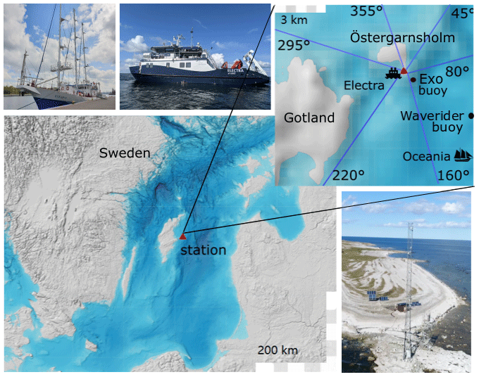
Figure 1This map shows the locations of the EC flux tower on the island of Östergarnsholm (red triangle) and the research vessels, along with the positions of the EXO2 multi-parameter sensor and waverider buoy. Reference pictures of the flux tower are also included. Wind sectors are identified based on the classification by Rutgersson et al. (2020). Map © BSHC.
2.1 EC aerosol flux tower
Stockholm University has installed a 12 m tower for measuring aerosol EC fluxes adjacent to the 30 m ICOS mast on Östergarnsholm, as shown in Fig. 1, which is used to measure EC greenhouse gas fluxes. A horizontal head ultrasonic anemometer (Gill HS, Gill Instruments Ltd, UK) was placed on a platform at the top of the aerosol flux tower, with the three-axis sonic head 12 m above the average sea surface level. Wind speed in three dimensions (u, v, w) and the atmospheric temperature derived from the speed of sound (Tair) were recorded at 20 Hz. The open side of the horizontal head faced south to maximize the quality of measurements in the open-sea sector (80–220∘).
A high-speed open-path H2O and CO2 sensor was mounted at 10.4 m height on a co-located mast with 8 m horizontal separation and recorded at 20 Hz (Licor-7500A, Li-Cor Environmental Ltd, UK).
Ambient air was sampled vertically downward through a 5 m long stainless-steel sampling line with a (6.35 mm) outer diameter (5.35 mm inner diameter). To prevent precipitation from entering the sampling line, a 180∘ bend was installed at the top of the sample line. The sampling line led to an OPC (model 1.109, Grimm Aerosol Technik GmbH, Germany) that sampled at 1.2 L min−1 and that was mounted on a second platform at 7 m height. The OPC was calibrated by Grimm Aerosol Technik GmbH, and its first-order response time (see Sect. A1.2) was measured at the Department of Environmental Science, Stockholm University. The OPC was set to count the aerosol number concentration Ni in 15 size classes i with diameters µm, with a time resolution of 1 s. Given the flow through the sample line and the dimensions of the tube, the flow in the sampling line should have been laminar ( 322), where Q is the sampling flow of the OPC, Dtube is the diameter of the sampling line, and ν is the kinematic viscosity.
Because access to the sampling site is limited and the amount of electrical power at the site is restricted, it was not possible to dry the aerosol sample. Therefore, the OPC conducted all measurements at ambient temperature and humidity. All the instruments were recorded and monitored using a gateway and PC running the LabVIEW software SCOL-EC developed by Stockholm University (Nilsson et al., 2021).
2.2 EC method and calculations
To estimate aerosol fluxes using the EC method, high-frequency measurements of aerosol number concentrations are correlated with the vertical wind speed w. These measurements are averaged over time, typically at 30 min intervals, to obtain the total and size-resolved net aerosol fluxes ( and ), represented here using overlines and primes (′) to denote the 30 min means and turbulent fluctuations, respectively. The net aerosol fluxes are a result of transport caused by both upward motions (emission fluxes) and downward eddy motions (deposition fluxes). However, only emissions from sources within the flux footprint will contribute to upward fluxes. Aerosol particles that originate outside the flux footprint will not have a positive correlation with the vertical wind component w and thus will not contribute to upward fluxes. Instead, they will contribute to downward fluxes through dry deposition. Therefore, by estimating the dry deposition flux and subtracting it from the net aerosol flux, it is possible to derive the SSA emission flux.
The CALCEDDY LabVIEW program, which was developed at Stockholm University (Nilsson et al., 2021), was used for eliminating spikes exceeding 6 times the standard deviation, double rotation of the coordinates, linear detrending of the data, correcting for lags (using a lag time ranging from 0 to 9 s with the largest correlation between N′ and w′), and calculating covariances, averages, and standard deviations.
2.3 EC footprint
In the simplest terms, the flux footprint refers to the area that the instruments on the tower “see”. It represents the area upwind of the tower within which aerosol fluxes are detected by these instruments. Under stationary conditions, the footprint represents the area from where the measured fluxes originate, whether they are fluxes of momentum, heat, gases, or aerosols. The size of the footprint depends on various factors, such as the measurement height zm, atmospheric stability , friction velocity u*, and wind direction. Several methods can be used to determine the footprint. In the case of Östergarnsholm, it has been thoroughly studied using backward dispersion modelling (Smedman et al., 1999) and flux footprint modelling (Gutiérrez-Loza et al., 2022). According to Högström et al. (2008), for measurements taken at a height of 10 m above the surface, 80 % of the fluxes originated 800 m upwind of the tower for unstable atmospheric stability conditions, 1500 m upwind of the tower for neutral atmospheric stability conditions, and 6500 m upwind of the tower for stable atmospheric conditions.
2.4 EC aerosol flux errors
In order to quantify aerosol fluxes using the EC approach, we need to consider potential measurement errors resulting from physical phenomena, instrument problems, and the specifics of our particular set-up. Although there are a number of potential flux errors, many can be prevented, minimized, or corrected. In this section, we introduce the different corrections we have applied to process our data. Further details can be found in Appendix A.
We distinguish between two types of errors: random stochastic errors (ϵ) and systematic errors (δ). For most systematic errors, there are established methods to estimate the error, which allows us to correct the measurements. In this study, systematic errors were calculated in MATLAB version 9.90.2037887 (R2022b) update 8 using the AERosol Eddy Covariance flux errors and corrections (AEREC) 2.0 code developed at Stockholm University. However, for random errors, we can only estimate the magnitude (ϵ) using statistical relationships. In the following, we provide a description of the errors that we have quantified, with an emphasis on aerosol flux errors.
2.4.1 Systematic EC aerosol flux errors
Systematic errors can result in a fixed bias, a relative bias that scales with the magnitude of what is being measured, or a bias that varies over time. In the EC flux system used in this study, the lateral separation between the sonic anemometer and the OPC results in a negligible error (δls), especially considering that the OPC data were only recorded at 1 Hz. We calculated aerosol EC fluxes for 30 min periods, which is a standard approach in many EC studies (e.g. Nilsson et al., 2001, 2021; Geever et al., 2005; Mårtensson et al., 2006; Ahlm et al., 2010). Although a low-cut frequency correction can be applied to account for very large eddies that are not completely sampled during 30 min periods, this issue is more likely to occur over continental sites under very unstable conditions. Since our dataset was obtained in the marine boundary layer under close-to-neutral conditions, this is unlikely to be a problem, and we have not applied this correction.
Differences in the properties of the footprint in the sectors surrounding the mast can also cause errors when the instantaneous wind direction changes during the 30 min flux periods. However, we will only consider data from the open-sea sector in our analysis, assuming that the surface properties of the footprint in this sector are fairly consistent.
Other systematic errors are large enough that we need to try to quantify them and correct the observed flux for these errors. These include the error introduced by flux losses at high frequency in closed-path systems, which is often referred to as low-pass filtering, i.e. signal damping in the sampling line to the OPC and the limited response time of the OPC. We also need to consider the effect of density fluctuations (Webb correction).
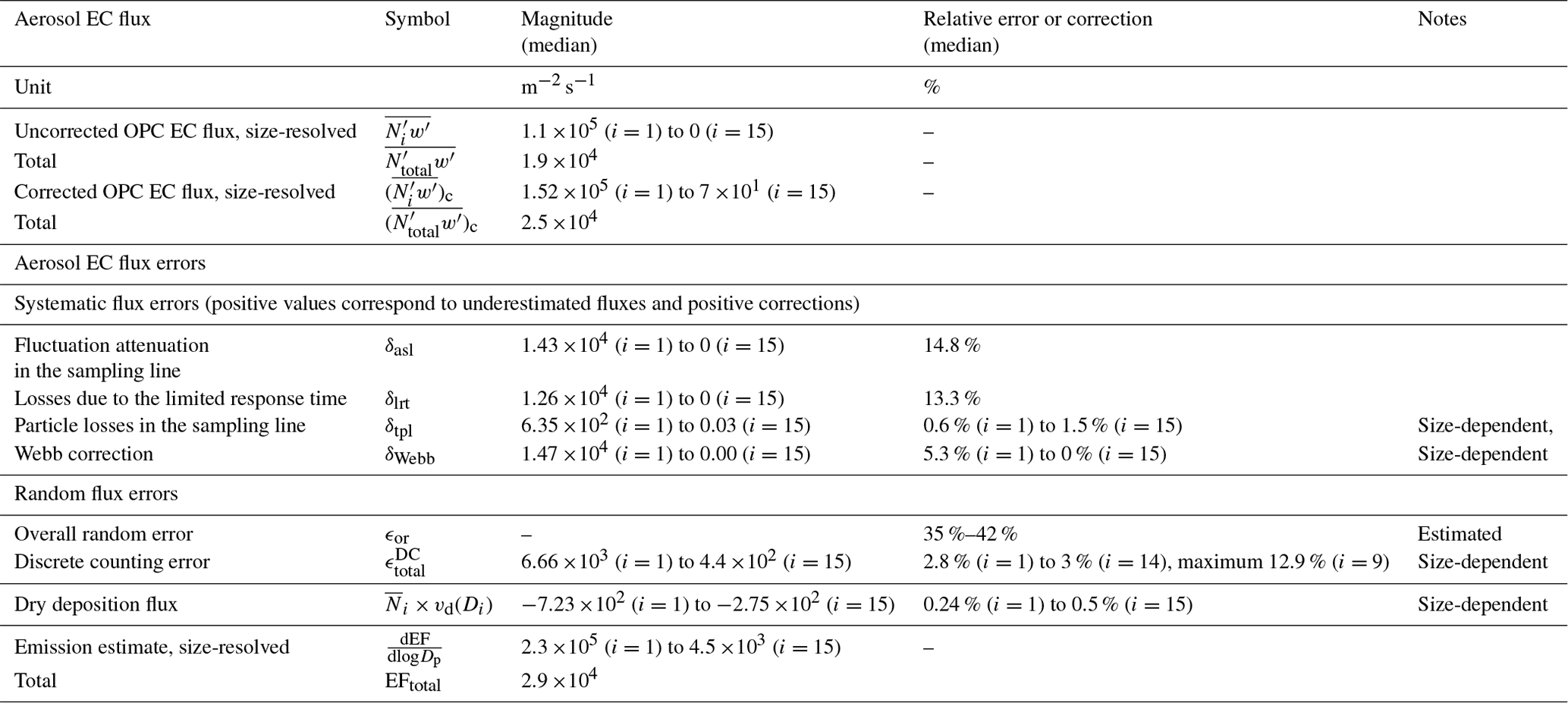
A short summary of systematic errors, along with their estimated magnitudes, is provided below in the order in which they were estimated and corrected. Table 3 in Sect. 3.2 summarizes the results (see also Fig. S1 in the Supplement). For a more detailed description of the error estimation and corrections, refer to Sect. A in the Appendix.
One of the largest sources of error results from the attenuation of turbulent fluctuations in the sampling line and the OPC, which leads to an underestimation of the EC flux that is almost constant across all the particle sizes (except for the largest size bins). This error is significant, corresponding to 14.8 % of the observed EC flux (see Table 3 and Fig. S1).
The impact of the limited response time of the OPC was estimated on the basis of Horst (1997). To include the smallest eddies in EC fluxes, instruments capable of high-frequency measurements (10–20 Hz) are required. However, since the OPC used in this study was only capable of making measurements at 1 Hz, there is a substantial attenuation of the flux in our measurements that is almost constant with size (except for the largest size bins). When normalized to the average total number flux, this error corresponds to 13.3 % of the total aerosol number flux (see also Fig. S1 and Table 3).
High-frequency losses were assessed using two different methods: (1) following the approach by Wolf and Laca (2007) and (2) comparing the co-spectrum to the co-spectrum of heat. The estimated high-frequency flux losses ranged from 1 % to 13.9 %.
Losses of aerosols due to particle diffusion, impaction, and sedimentation within the sampling line can lead to an underestimation of the measured aerosol number concentration that varies with particle size. To estimate these losses, we used a program developed by Hsieh (1991). Since we minimized the bends and the length of the sampling line to the OPC and since most of the particles measured by the OPC fall within the accumulation mode, the losses in the sampling line were relatively small. When normalized to the average total number flux, the errors due to losses in the sampling range were from 0.6 % for the smallest OPC size bin centred at Dp=0.265 µm to 1.5 % for the largest OPC size bin centred at Dp=2.24 µm (see Fig. S1 and Table 3).
To account for the influence of water vapour fluxes on scalar concentrations of interest relative to total moist air, a correction known as Webb correction is required (Webb et al., 1980). This error accounted for 5.3 % relative error in the smallest size bin to 0 % in the largest size bin (see Table 3 and Fig. S1). One possible explanation for the small magnitude of this correction is the damping of density fluctuations in the sampling line. This aligns with the observations of Yang et al. (2016), who noted a significant dampening of water vapour fluctuations in their sampling lines.
2.4.2 Random EC aerosol flux errors
Random errors are dependent on the sample size, and as such a higher number of data points result in smaller random errors because they average out. When calculating EC fluxes, it is essential to consider a number of random errors, including variations in the prevailing wind direction and resulting differences in footprint properties during the 30 min averaging periods. However, as mentioned previously, we only considered fluxes obtained during periods when the wind blew from the open-sea sector, assuming that the footprint surface properties were similar across this sector.
For particle-counting instruments such as OPCs and CPCs, a fraction of the random error is related to the discrete counting of the particles. The discrete counting error increases with increasing particle size and decreasing particle concentration. In the case of this dataset, the discrete counting error accounted for a relative flux error of ∼ 3 % (maximum ∼ 12.9 % at Dp=1.5 µm). The random error was determined to vary between 35 % and 42 %, obtained by shifting N′ and w′ by 3 min and 5 min, respectively, and calculating the standard deviation of the computed co-variance. Unlike systematic errors, random errors cannot be corrected, and instead we will indicate them as error bars in the following data analysis.
2.5 Estimation of sea spray aerosol emission fluxes using an aerosol dry deposition model
To estimate the actual SSA emissions, we need to model the dry deposition fluxes and subtract them from the corrected net aerosol fluxes. To do so, we use
Here vd is the size-dependent aerosol dry deposition velocity for each size bin diameter Di, following the approach of Nilsson et al. (2001) and Nilsson et al. (2021). We use the parameterization of dry aerosol deposition by Schack Jr. et al. (1985) for vd, set for the wind tunnel parameters corresponding to water surfaces at ms−1. Therefore, the emission flux for the entire OPC size range is
2.6 Spectral analysis
To identify EC data points that should be excluded from the analysis, we calculated the turbulence power spectra and co-spectra using a fast Fourier transform (FFT) for each 30 min time period. The power spectra and co-spectra were frequency-weighted and normalized by the variance or covariance, respectively. We excluded a 30 min period if the slope of the power spectrum deviated notably from on the normalized scale in the inertial sub-range or if the slope approached +1 (white noise) at a frequency lower than the expected response time of the instrument. Similarly, we excluded a 30 min period if the slope of the co-spectra deviated notably from the slope. We divided the 30 min time periods into three categories: (A) good data, (B) non-ideal data, and (C) poor data. Examples of the power spectra and co-spectra for aerosol, temperature, horizontal wind speed, and water vapour fluxes for “good data” are presented in Fig. S2. As can be seen in Fig. S3, the impact of the spectral analysis on the size-resolved fluxes was small. In the following analysis, we used only data from 30 min periods that were classified as “good”.
2.7 Production of nascent SSA using a laboratory sea spray simulation chamber
A laboratory sea spray simulation chamber was used to generate nascent SSA during two research cruises in the vicinity of Östergarnsholm. R/V Oceania was stationed there from 19 May 2021 at 16:00 to 22 May 2021 at 00:00 (local time, LT) and again from 23 May 2021 at 00:00 to 24 May 2021 at 04:00 LT. R/V Electra was also in the area from 10 August 2021 at 09:30 to 22 August 2021 at 08:00 LT but had to leave its anchored position on 16 August at 08:00 LT to return to the harbour in Fårösund for refuelling due to poor weather conditions. The ship returned to Östergarnsholm on 18 August at 08:00 LT, but it was not possible to anchor in the same position, and the ship had to return to the nearby harbour each evening (17:00–08:00 LT) until the end of the campaign. Therefore, in the following sections, we only include chamber measurements obtained when the ship was located close to the station on Östergarnsholm.
The sea spray simulation chamber used for the experiments is described in detail in Salter et al. (2014). In summary, SSA particles were generated by a plunging jet that hits the water surface from a height of 40 cm, entraining air into the water. The entrained air rises in the form of bubbles that burst and expel droplets, which are eventually dried and sampled into aerosol instrumentation. The sea spray simulation chamber operates under a slight positive pressure by introducing particle-free sweep air to exclude the possibility of outside air contamination and to ensure that the headspace of the chamber is well-mixed. Although the chamber can be temperature-controlled, it was operated without temperature control in this study because the seawater in the chamber was constantly being replaced and thus was at ambient temperature. This makes our experiments comparable to previous chamber experiments that used a plunging jet and fresh seawater (e.g. Facchini et al., 2008; Hultin et al., 2010, 2011; Zábori et al., 2012, 2013). The chamber was continuously filled with local surface seawater sampled using the seawater inlets of the ships. During the R/V Oceania campaign, inline measurements of seawater temperature, Tseawater, and salinity, S, were made using a seabird conductivity–temperature–depth (CTD) probe (SBE 21 SeaCAT Thermosalinograph, Sea-Bird Scientific, USA) and oxygen saturation was measured with an oxygen meter (Fibox 4 trace, PreSens Precision Sensing GmbH, Germany). During the R/V Electra campaign, the seawater temperature in the chamber was continuously measured using a conductivity sensor (model number 4120, Aanderaa, Norway) and the dissolved oxygen (DO) concentrations in the chamber were measured with an oxygen optode (model number 4175, Aanderaa, Norway). The concentrations of chlorophyll α and fluorescent dissolved organic matter (FDOM) were measured inline with two fluorometers (Cyclops-7F, Turner Designs, USA). Additionally, we utilized salinity data measured by an EXO2 multi-parameter sensor (YSI Inc., Yellow Springs, OH, USA) installed on a mooring 1 km south-east of the station by Uppsala University. Measurements of wave properties were made with a Directional Waverider moored at a depth of 39 m, 4 km south-east of the tower. For more details on the wave measurements, we refer the reader to Rutgersson et al. (2020) and Hallgren et al. (2022).
2.7.1 Measurements of the aerosol size distribution
The size distribution of the aerosols produced in the chamber was measured using a custom-built differential mobility particle sizer (DMPS), which consisted of a Vienna-type differential mobility analyser (DMA) and a condensation particle counter (CPC, model 3772, TSI, USA) with a flow rate of 1 L min−1 that measured particles with electrical mobility diameters between 0.015 and 0.906 µm distributed over 37 size bins. We also used a white-light optical particle size spectrometer with a flow rate of 5 L min−1 (WELAS 2300 HP sensor and Promo 2000 H, Palas GmbH, Germany, hereafter called WELAS), which measured particles with optical diameters between 0.150 and 10 µm distributed over 59 bins. To combine the size distributions measured by the DMPS and WELAS, we have converted the optical diameters measured by WELAS to volume-equivalent diameters assuming a refractive index of for sea salt particles, which corresponds to the value of NaCl (Abo Riziq et al., 2007). We carried out the conversion using the software provided by the manufacturer (PDAnalyze Version No. 2.024, Palas GmbH, Karlsruhe, Germany), which was based on instrument-specific Mie calculations. The diameters of the aerosol particles were also shape-corrected according to Zieger et al. (2017). Before sampling, we dried the particle-laden air in two Nafion dryers (model MD-700-36F/48F, Perma Pure, USA) that were horizontally mounted in front of the DMPS and WELAS. We monitored the temperature and relative humidity (RH) of the sample with two sensors (HYTELOG-USB, B+B Thermo-Technik GmbH) mounted in front of the sampling inlets of the WELAS and DMPS system to ensure that the measured particle diameters could be considered dry diameters. The average RH (measured behind WELAS) was 31.7±2 % for the Oceania campaign and 18.9±1.6 % for the Electra campaign (mean ± standard deviation).
To estimate losses in the sampling lines we used the Particle Loss Calculator Software (von der Weiden et al., 2009). After correcting for all factors, we combined the DMPS and WELAS data at measured particle sizes of 0.35 µm. All sizing instruments were calibrated with polystyrene latex spheres.
2.7.2 Derivation of SSA production fluxes from the chamber measurements using the continuous whitecap method
To estimate the production flux of SSA particles using chamber measurements, we employed the continuous whitecap method (CWM, e.g. Cipriano and Blanchard, 1981; Mårtensson et al., 2003). The CWM combines an estimate of the size-resolved number of SSA particles produced per unit of whitecap area per second in the chamber with an estimate of whitecap coverage to predict the size-resolved interfacial number of SSA particles per unit of ocean surface area per unit of time (Lewis and Schwartz, 2004).
One of the most widely used sea spray source functions is based on the discrete whitecap method (DWM, Monahan and O'Muircheartaigh, 1980). This source function combines laboratory experiments that measured the size-resolved number of SSA particles produced by a simulated breaking wave and the oceanic whitecap coverage (W), which are often parameterized in terms of the wind speed at 10 m above the sea surface (U10 m). For example, Monahan and O'Muircheartaigh (1980) used the following empirical relationship:
It is important to note a key difference between the CWM we used and the DWM developed by Monahan and colleagues (e.g. Monahan and O'Muircheartaigh, 1980). The goal of the DWM, as originally formulated, was not to determine the number of SSA particles produced per unit of whitecap area per second. Instead, this approach aimed to determine the number of SSA particles produced per unit whitecap area from a laboratory-simulated breaking wave over the entire lifetime of the resulting whitecap and the associated degassing bubble plume. See Callaghan (2013) for a detailed discussion of this.
To calculate the SSA production flux , we multiply the flux per whitecap area by the whitecap coverage using the following equation:
where is the measured size distribution, Qsweep is the sweep flow, and Asurface is the seawater surface area inside the chamber covered by bubbles. However, our experimental set-up has a limitation: we did not determine the exact surface area of seawater covered by bubbles. For future research, we recommend measuring both air entrainment and the fraction of the water surface within the chamber covered by bubbles to improve flux estimates through this scaling approach. As an approximation, we estimated the fraction of the water surface covered by bubbles in previous experiments with artificial seawater at a salinity of S=35 g kg−1, C, and Qjet=1.75 L min−1 (Salter et al., 2014). These authors used a wide-angle lens to photograph the water surface inside the chamber, determining that approximately 6 % of the surface was covered by bubbles. Since these photos were taken at higher salinities, with an expectation of more and smaller bubbles, we adjusted the estimate, resulting in whitecap coverages of 2 % and 3 % for the Electra campaign at flow rates of 1.3 and 2.6 L min−1, respectively. Considering the Oceania campaign's significantly higher jet flow rate (3.5 L min−1) leading to increased bubble formation, we estimate that 21 % of the water surface in the chamber was covered by bubbles during this campaign. Those whitecap coverage estimates were determined by comparing the flux that would result from 100 % whitecap coverage to the magnitude of the emission fluxes derived from the EC measurements in the overlapping size range.
2.7.3 Derivation of SSA production fluxes from the chamber measurements using air entrainment
Another method for obtaining estimates of the production flux of SSA particles from breaking waves and whitecaps using sea spray simulation chambers has been developed by Long et al. (2011) and Salter et al. (2015). These authors combined the number of particles produced per unit time in a logarithmic interval of Dp with measurements of air entrainment or detrainment. This approach assumes that all air entrained into the water column detrains as bubbles that produce particles and does not consider other factors that may affect the air entrainment flux, such as breaking wave strength or sea state.
To apply this approach, we measured the volume of air entrained in a manner similar to Salter et al. (2014) under conditions relevant to our field measurements, using seawater from the footprint area (S=6 g kg−1, C, and C, respectively, for the May and August campaigns). To measure the volume of air entrained by the plunging jet, we enclosed the jet in a stainless-steel tube, with the base of the tube submerged 10 mm below the seawater surface, and recorded the volumetric air flow 30 times using a flow meter (Gillibrator 2, Sensidyne, USA). Using these estimates of air entrainment, Qair, we can estimate the particle production rate f (per cubic metre) as follows:
The size-resolved interfacial flux is then obtained by multiplying the particle production rate by a parameterization of the air entrainment flux (Long et al., 2011):
2.7.4 Derivation of SSA production fluxes by scaling size-resolved chamber measurements to ambient fluxes
Combining EC flux measurements with chamber measurements enables us to estimate the sea spray source across the full particle size range. To achieve this, we compared the aerosol number concentration (Nj) measured in the sea spray simulation chamber across WELAS size bins (j) with the vertical aerosol number flux () from the EC flux system over size bins (i) and obtained a scaling factor. Because the WELAS operating on the sea spray chamber and the Grimm OPC-measuring EC fluxes on the tower are different and operate using different size bins, we interpolated the WELAS data to the EC flux OPC data range ( µm) using the MATLAB spline function. This enabled us to estimate the ratio (R) of the EC flux to the concentration of particles measured in the sea spray simulation chamber (SSSC):
where has the unit metre per second.
It is important to note that the particles produced in the chamber experiments were dried before being sized and counted by DMPS and WELAS, while the EC flux OPC measured particles at ambient RH ≈80 %. For comparability, we have converted all diameters to radii at RH =80 % and referred to them as R80, unless explicitly stated otherwise. We used only the flux measurements obtained simultaneously with the chamber experiments to scale the chamber data.
3.1 Synoptic-scale and micro-meteorological overview
Figure 2 displays a time series of micro-meteorological and synoptic parameters including wind speed, direction, friction velocity, air temperature, and RH as well as ambient aerosol concentrations and net fluxes from all the sectors. The fluxes from the coastal-influenced sector, which were excluded from the analysis, are indicated in grey. Upward aerosol fluxes dominated during both campaigns, with 491 half-hour periods being dominated by upward aerosol fluxes and 157 half-hour periods being dominated by downward aerosol fluxes across both campaigns.
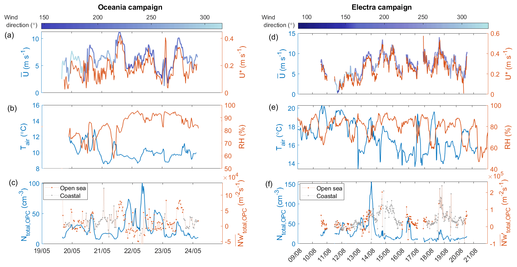
Figure 2Time series of relevant micro-meteorological and aerosol parameters for the Oceania and Electra campaigns. Panel (a) displays wind speed and direction as well as the friction velocity for the Oceania campaign. Panel (b) displays air temperature and relative humidity for both campaigns. Panel (c) shows the ambient particle concentration (NOPC) and net fluxes measured on Östergarnsholm during the Oceania campaign. Panels (d) to (f) show the same parameters as panels (a) to (c) but for the Electra campaign.
Table 1 provides an overview of synoptic-scale atmospheric and seawater properties, including wind speed and direction, fetch, atmospheric pressure, air and seawater temperature, salinity, concentration of dissolved oxygen, and chlorophyll α in seawater, during the two campaigns. Frequency histograms of these parameters for both campaigns are also presented in Figs. S4 and S5. Additionally, wind roses of the prevailing wind directions and wind speeds during both campaigns are shown in Fig. S6. Measurements at the site indicated that, during both campaigns, the air mainly came from the west to south-west, accounting for 85 % of the measurement time. Back-trajectories with endpoint heights at 100 m were computed using the HYSPLIT model for both campaigns (Stein et al., 2015; Rolph et al., 2017) and are presented in Figs. S7 and S8.
Table 1Overview of synoptic-scale atmospheric and seawater properties during the two campaigns, presented as the mean and standard deviation of values.
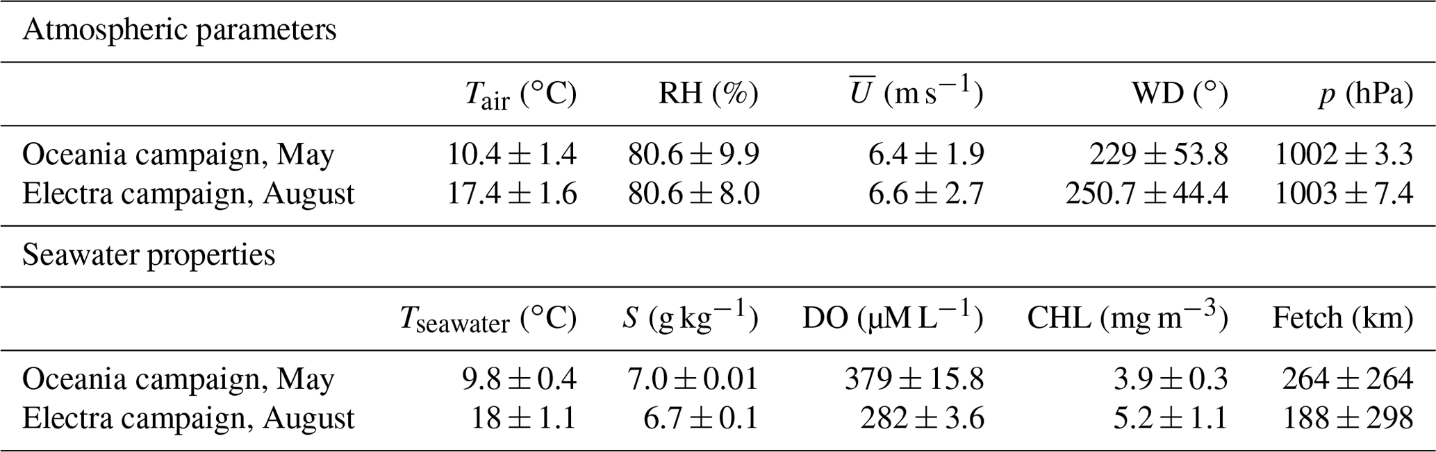
During periods with southerly winds, the distance the sampled air mass spent above open water ranged from 500 to 1200 km, with the highest values observed during the Electra campaign. The local wind speed (averaged over 30 min intervals) ranged from 0 to 14 m s−1 but was mostly between 4 and 10 m s−1 (see Fig. 2 and Table 1). A clear seasonal increase in seawater and air temperature was observed between May and August. As a proxy for phytoplankton biomass, chlorophyll α (CHL) was used. The Oceania campaign in May fell between the spring and summer blooms, while the Electra campaign in August coincided with the late stages of the summer bloom. Therefore, it is not surprising that higher levels of chlorophyll α were measured during the Electra campaign (see Table 1).
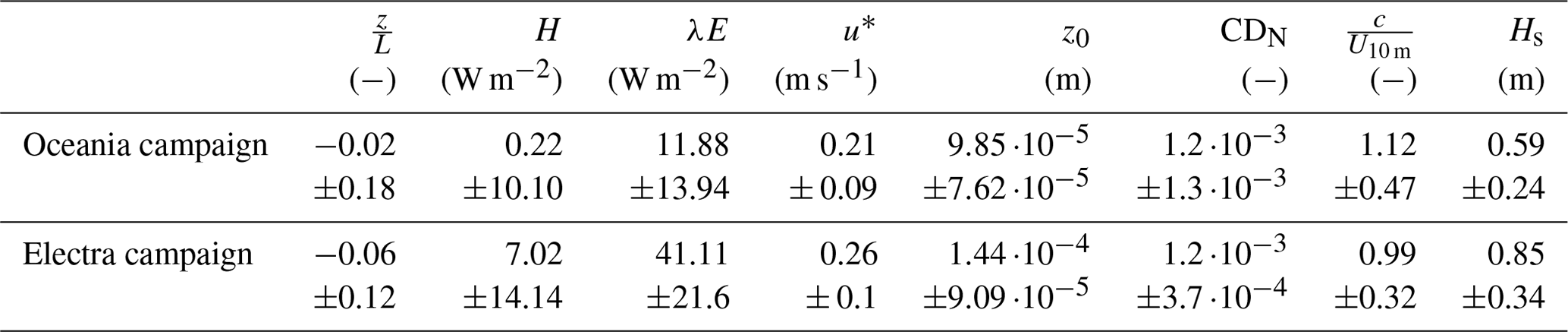
Table 2 and the histograms in Fig. S9 provide an overview of the micro-meteorological conditions encountered during both campaigns in the open-sea sector. The mean stability was close to neutral during both campaigns with values of −0.02 ± 0.18 during the May campaign and −0.06 ± 0.12 during the August campaign. Stability affects the turbulent exchange of heat and water vapour, where unstable conditions lead to enhanced turbulence and stable conditions suppress turbulent exchange (see also Svensson et al., 2016, for stratification characteristics). This is also reflected in the latent and sensible heat fluxes. Sensible heat fluxes in the open-sea sector were close to zero during the May campaign (0.22 ± 10.1 W m−2) and upward during the August campaign (7.02 ± 14.14 W m−2). The latent heat fluxes were higher in August than in May (11.9 ± 13.9 W m−2 in the open-sea sector in May compared to 41.1 ± 21.6 W m−2 in August), which can be explained by increased evaporation as a result of higher seawater temperatures in August. Similar patterns in stability and latent or sensible heat exchange have previously been observed at Östergarnsholm (Rutgersson et al., 2020). The mean friction velocity for the open-sea sector was 0.21 m s−1 during the May campaign and 0.26 m s−1 during the August campaign, which agrees well with the measurements reported in Rutgersson et al. (2020). Since variations in micro-meteorological parameters in the open-sea sector were small between the two campaigns (except for the heat fluxes), we have combined these datasets in the analysis that follows.
Table 2Overview of the micro-meteorological conditions encountered during both campaigns in the open-sea sector (80–220∘). The values are presented as a mean and standard deviation. The table includes sensible heat flux H, latent heat flux λE, neutral drag coefficient (CDN), wave age (), and significant wave height (Hs).
A description of the diurnal cycles of the ambient aerosol concentration and fluxes, as well as the micro-meteorological parameters and seawater properties mentioned above, is also provided in Sect. S1 in the Supplement.
3.2 Ambient aerosol concentrations and fluxes
In total, we obtained 648 half-hour estimates of the net aerosol flux by combining the data from the two campaigns, of which 386 originated from the open-sea sector. After excluding data periods characterized as non-ideal or poor, based on spectral quality control and data points when the ships were not located close to the station, we were left with 203 half-hour periods.
Figure S1b shows the size-resolved aerosol net fluxes () before and after applying all corrections. Additionally, it shows the aerosol emission flux derived from the corrected net aerosol flux after subtracting the aerosol dry deposition flux.
As shown in Table 3, the median uncorrected net flux was 1.9⋅104 m−2 s−1, which increased to 2.5⋅104 m−2 s−1 after applying all the corrections. The estimated median total dry deposition flux was 2.9⋅102 m−2 s−1, several orders of magnitude lower than the SSA emission flux (∼ 1 %), which was estimated to be 2.9⋅104 m−2 s−1 (median of the integrated fluxes across all OPC size bins). However, the dry deposition is still significant for the largest size bins. Previous studies over the open sea have estimated deposition fluxes of between 14 % (Yang et al., 2019) and 30 % of the net flux (Geever et al., 2005; Nilsson et al., 2021).
Table 3The table presents the median values of the uncorrected and fully corrected net aerosol number fluxes, along with the systematic and random aerosol errors. In addition, the table shows the modelled aerosol dry deposition flux and the estimated emission flux. The OPC bins are labelled as .
Similar to a previous study in this region (Nilsson et al., 2021), the correction for aerosol losses in the sampling line and the correction that accounts for dry deposition fluxes had only minor impacts on total and size-resolved fluxes. This is likely because the OPC mostly samples the accumulation mode, where deposition in sampling tubes or surfaces within the flux footprint is minimal.
3.2.1 Dependence of aerosol net fluxes on the micro-meteorology
The correlations between the measured net aerosol fluxes and micro-meteorological parameters, such as drag coefficient, roughness length, friction velocity, stability, sensible and latent heat flux, as well as turbulent kinetic energy, are shown in Fig. 3. The net aerosol fluxes demonstrate positive correlations with the wind speed, roughness length, friction velocity, turbulent kinetic energy, significant wave height, and wave Reynolds number and a negative correlation with wave age. In the following sections, we will focus on the dependence of the emission flux on the wind speed U10 m, significant wave height Hs, and wave Reynolds number , which was calculated based on Zhao and Toba (2001) (νw represents the viscosity of water and was calculated for the average seawater temperature and salinity encountered during this study).
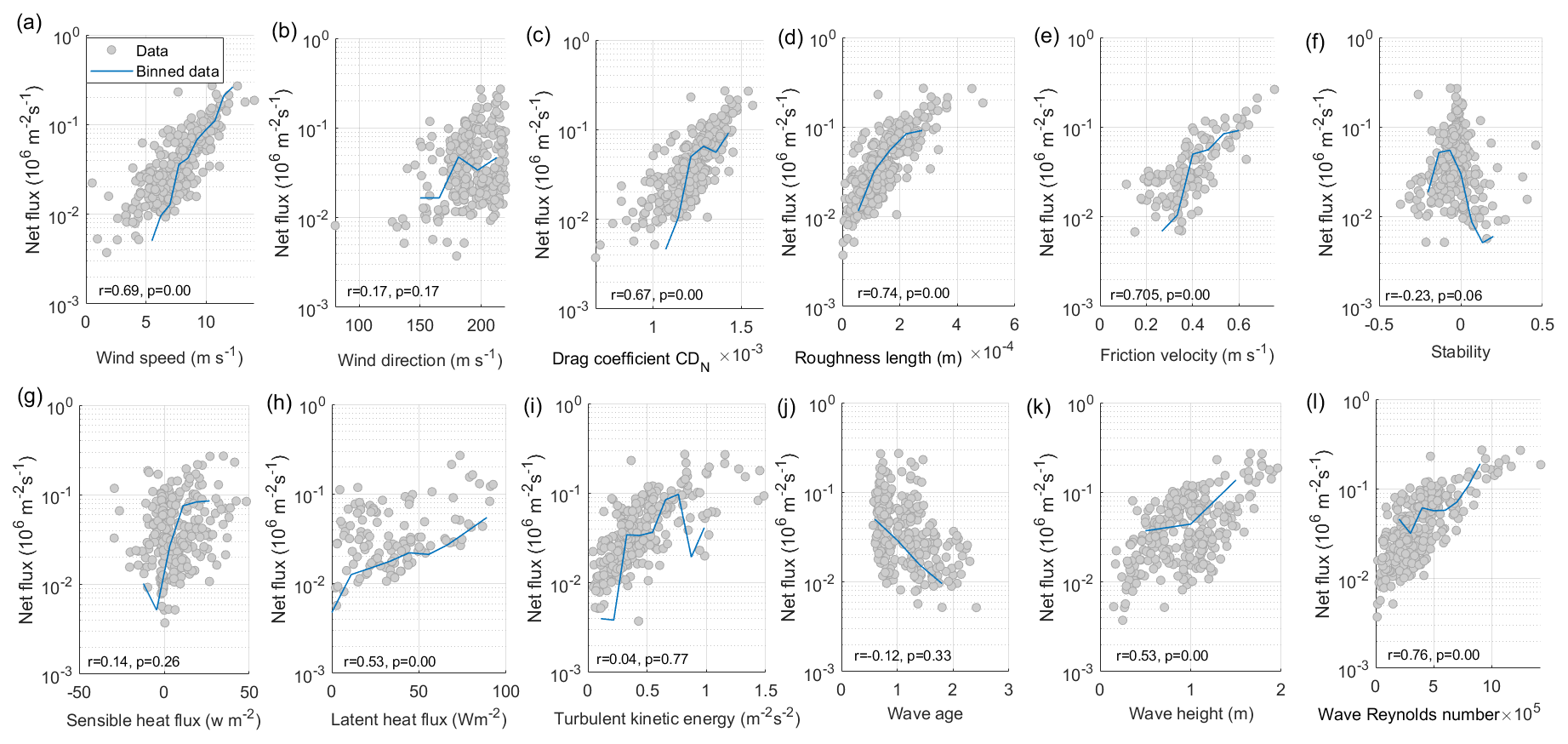
Figure 3Scatterplots of the net aerosol flux from the open-sea sector with (a) wind speed U10 m, (b) wind direction, (c) drag coefficient CDN, (d) roughness length z0, (e) friction velocity u*, (f) stability , (g) sensible heat flux H, (h) latent heat flux λE, (i) turbulent kinetic energy, (j) wave age, (k) wave height, and (l) wave Reynolds number. The grey dots show all the data points, and the blue lines show binned data. The correlation coefficients r and levels of significance p for each parameter with the EC flux are given in each panel.
3.2.2 Dependence of aerosol emission fluxes on wind speed
As shown in Fig. 4a, the SSA emission fluxes exhibit a logarithmic increase with a linear increase in wind speed:
which is consistent with the findings of many previous studies (Nilsson et al., 2001; Geever et al., 2005; Norris et al., 2008, 2012; Yang et al., 2019; Nilsson et al., 2021).
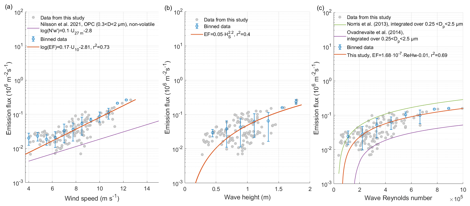
Figure 4SSA emission flux versus (a) wind speed ≥4 m s−1, (b) significant wave height, and (c) wave Reynolds number. The grey dots represent the 30 min emission fluxes, while the blue lines represent binned data (mean and standard deviation) and the orange lines represent fits to the individual 30 min data periods. Additionally, we compare our results to those from previous studies.
We have included the fit for the relationship between wind speed and net flux from a coastal site in the Baltic Sea reported in Nilsson et al. (2021) for comparison.
Factors such as aerosol dry deposition fluxes, boundary layer height, salinity, seawater temperature, fetch, sea ice fraction, seawater depth, wave field, and the presence of surfactants at the seawater surface can affect the slope and intercept of the fit in Fig. 4a. Furthermore, the fit parameters are dependent on particle size. Figure S10 shows that a log-linear relationship between SSA fluxes and wind speed can also be observed in each separate size bin of the OPC. The slopes a, intercepts b, and coefficients of determination r2 for the size-resolved SSA emission fluxes are presented as a function of aerosol size in Fig. S11. The change in slope with size provides an estimate of the number of additional particles per surface area and second that are emitted for the same change in wind speed, with the highest increase observed for particle diameters between 0.3 and 1 µm, where the correlation coefficients are highest. Since particles of this size likely originate as film drops, this indicates that film drop production is potentially more sensitive to changes in wind speed than jet drop production under the conditions in which our measurements were made. When comparing the fits of the separate size bins to the findings from Norris et al. (2008), we note a reasonable agreement with the slopes of the fits observed in their study except for the largest size bin.
3.2.3 Dependence of aerosol emission fluxes on wave properties
Figure 4b and c present a comparison between the aerosol emission and two wave parameters, significant wave height Hs and wave Reynolds number ReHw. Binning the data into regularly distanced intervals based on the median values reveals trends. The emission flux shows a power-law increase with increasing significant wave height, which is similar to the relationship reported by Yang et al. (2019) (although their emission flux was more than an order of magnitude higher since they used a CPC to measure the SSA emission fluxes for particles Dp>100 nm). Additionally, there is a linear increase in the emission flux with increasing wave Reynolds number, which agrees very well with the parameterizations by Norris et al. (2013) and Ovadnevaite et al. (2014).
In their study, Yang et al. (2019) observed that higher values of U10 m and Hs resulted in higher size-resolved aerosol emission fluxes across all the aerosol sizes ( µm). The effect was found to be stronger for Hs than for U10 m. In Fig. 5 we present our own findings on how size-resolved aerosol emission fluxes depend on U10 m, Hs, and ReHw and compare them to the results of Ovadnevaite et al. (2014). Note that we did not include the data from Yang et al. (2019) in Fig. 5 since their flux measurements were several orders of magnitude higher than ours, likely for the reasons outlined earlier.
We found that our sea spray aerosol emissions, like those reported by Yang et al. (2019), are strongly influenced by the significant wave height Hs. Specifically, we observed a significant difference in size-resolved aerosol fluxes of a factor of 1–3 depending on the size bin (at a probability value of p=0.0003 and at a significance level of 5 %) for m and m. Similarly, the data from Yang et al. (2019) differed by a factor of 1–5 for the same wave height ranges. Moreover, for wind speeds U10 m<5 m s−1 and U10 m>9 m s−1, we found a difference in aerosol flux of more than an order of magnitude (at a probability value of p=0.0002 and at a significance level of 5 %), while Yang et al. (2019) reported a much smaller difference, even over a wider range of U10 m.
Finally, from Fig. 5c, it is apparent that the wave Reynolds number strongly affects the size-resolved aerosol emission fluxes that we observed. In this regard, our dataset exhibits a similar trend compared to the parameterization of Ovadnevaite et al. (2014).
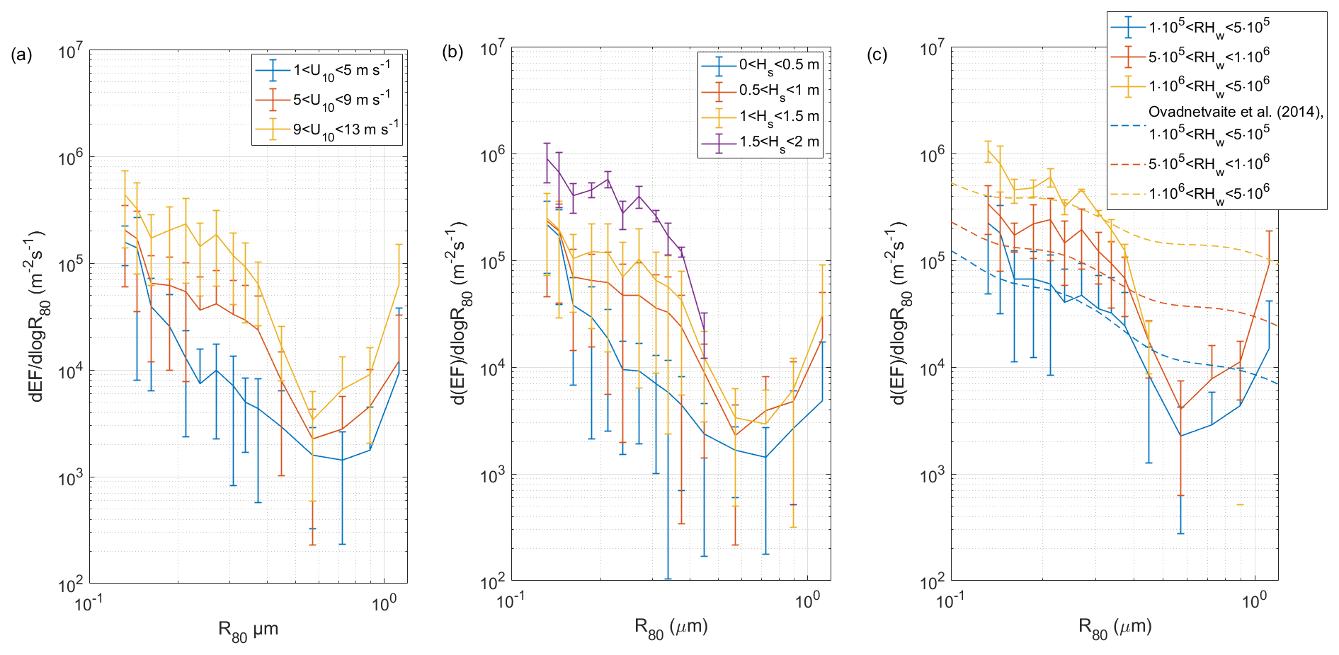
Figure 5Size-resolved emission flux dependence on (a) wind speed, (b) significant wave height, and (c) wave Reynolds number compared to the parameterization from Ovadnevaite et al. (2014). Values are presented as a mean and standard deviation.
3.3 Simulated sea spray production in the chamber experiments with water from the footprint area
Figure 6 shows a time series of the particle concentration measured in the headspace of the sea spray simulation chamber as well as flux estimates derived from the entrainment method from the continuous whitecap method and from scaling the chamber data to in situ fluxes. The figure also includes seawater properties such as seawater temperature, salinity, chlorophyll α, and dissolved oxygen, which were monitored during both the Oceania and Electra campaigns. Periods when the research vessels were not anchored close to the station were excluded, while periods when the wind was blowing from outside the open-sea sector are shaded.
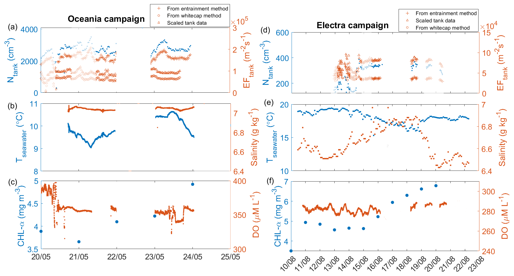
Figure 6Time series of various measurements from the sea spray simulation chamber during the Oceania and Electra campaigns. Panel (a) displays the particle concentration measured in the headspace of the sea spray simulation chamber, along with flux estimates derived from the entrainment method, the continuous whitecap method, and scaling the chamber data to the in situ fluxes. Shaded periods indicate when the ship was not anchored close to Östergarnholm or when the wind was blowing from outside the open-sea sector. Panels (b) and (c) show the seawater temperature and salinity and the concentrations of chlorophyll α and dissolved oxygen for the Oceania campaign, respectively. Panels (d–f) display the same measurements as panels (a–c) but for the Electra campaign.
When contrasting the data between the two campaigns, it is crucial to highlight that the experiments conducted in the Oceania campaign involved a higher plunging jet flow rate (3.5 L min−1 as opposed to 1.3 and 2.6 L min−1 during the Electra campaign). Consequently, this resulted in elevated particle concentrations recorded during the Oceania campaign. The sudden increase in particle concentration on 14 August was due to an increase in the plunging jet flow rate from 1.3 to 2.6 L min−1. Another factor that may have contributed to the higher particle concentration measured during the Oceania campaign is the lower seawater temperatures in May (around 10 ∘C) compared to August (around 17 ∘C). Previous studies have observed an increase in particle production at lower seawater temperatures (e.g. Woolf et al., 1987; Bowyer et al., 1990; Mårtensson et al., 2003; Sellegri et al., 2006; Zábori et al., 2012; Salter et al., 2014, 2015; Nielsen and Bilde, 2020; Zinke et al., 2022). In contrast, other studies (e.g. Schwier et al., 2017; Forestieri et al., 2018) have reported an increase in particle production with increasing seawater temperatures. Nevertheless, considering the relatively limited range of seawater temperatures examined in this study, the influence of seawater temperature is anticipated to be minor when compared to the impact of the jet flow rate.
Salinity was fairly constant during both campaigns (6.4–7 g kg−1). As the solubility of oxygen in water decreases with increasing temperatures, it is not surprising that the dissolved oxygen concentrations during the May campaign were higher than during the August campaign. Additionally, the concentration of chlorophyll α was higher during the August campaign. Chlorophyll α is often used as a proxy for biological productivity, which in turn can influence the concentration of dissolved oxygen through photosynthesis and respiration.
Figure S12 shows the mean number size distribution and total concentration of SSA particles in the headspace of the sea spray simulation chamber measured by DMPS and WELAS at different jet flow rates during both campaigns. It is evident from this comparison that the total number of particles produced in the sea spray chamber increased with an increasing jet flow rate, while the size distribution remained constant at each respective jet flow rate, with a mode centred at ∼ 100 nm and a second mode with a smaller magnitude centred at ∼ 500 nm. This aerosol size distribution is similar to the size distribution of inorganic sea salt measured with the same experimental set-up at S=6 g kg−1 (Zinke et al., 2022).
For the range of particle sizes where both DMPS and WELAS conducted measurements with a 100 % counting efficiency (i.e. between 0.3 and 0.8 µm dry diameter), the measurements were found to be in good agreement. This justifies our decision to combine the data from the two instruments at a dry diameter of 0.35 µm.
In a previous study, Hultin et al. (2010) used a sea spray simulation chamber that was similar to the one used in this study but smaller. They also continuously replaced the seawater in their chamber with fresh local seawater and observed a dependence of the SSA size distribution measured in the headspace of their chamber on wind speed and dissolved oxygen concentration. Following their example, we investigated whether wind speed and dissolved oxygen saturation could potentially influence the size distribution and overall concentration of SSA produced in our chamber. To do so, we binned the data into three wind categories (0–5, 5–10, and > 10 m s−1) and with respect to dissolved oxygen into subsaturated (DO<98 %), saturated (), and supersaturated (DO>102 %) seawater.
In contrast to Hultin et al. (2010), we observed no significant differences in the size-resolved particle concentration at different wind speeds (p>0.7 at a significance level of 5 %) or varying DO saturations (p>0.96 at a significance level of 5 %) (see also Figs. S13 and S14). We only observed a weak positive correlation between wind speed and total particle concentration for the Electra campaign (r=0.22, p=0.14 at Qjet=1.3 L min−1 and r=0.28, p=0.009 at Qjet=2.6 L min−1) but no significant correlation for the Oceania campaign (r=0.01, p=0.89). Moreover, we observed only a weak negative correlation between the total particle concentration in the headspace of the simulation chamber and the concentration of chlorophyll in the seawater (, p=0.16 at Qjet=1.3 L min−1 and , p=0.14 at Qjet=2.6 L min−1) and a weak positive correlation between the total particle concentration in the headspace of the simulation chamber and the concentration of FDOM in the seawater (r=0.23, p=0.15 at Qjet=1.3 L min−1 and r=0.16, p=0.14 at Qjet=2.6 L min−1) during the Electra campaign. Unfortunately, we did not have sufficient data points of chlorophyll α and FDOM concentration for the Oceania campaign to derive a correlation. Scatterplots for these parameters versus particle concentration are shown in Fig. S15.
3.4 Scaling the sea spray simulation chamber measurements to aerosol emission fluxes
We used three different approaches to convert the particle concentration measured in the headspace of the simulation chamber to emission fluxes. The first approach involved using the CWM (described in detail in Sect. 2.7.2), while the second approach used air entrainment measurements to derive SSA emission fluxes (explained in Sect. 2.7.3). The third approach, which we adapted from Nilsson et al. (2021), involved scaling the particle concentrations measured in the simulation chamber headspace to the in situ emission fluxes in the particle size range where both the WELAS and Grimm OPC used in the EC flux system conducted measurements (detailed in Sect. 2.7.4).
To calculate the average scaling factor for all size bins µm, it is necessary to have a similar slope between the chamber headspace number size distribution over and the flux distribution over . To test for this similarity, we conducted a Kolmogorov–Smirnov test (Massey Jr., 1951) on the particle size range µm. The test revealed that the slopes were not significantly different at a probability value of p=0.93 and at a significance level of 5 %.
Scaling the sea spray simulation chamber data to the in situ fluxes we measured in this study allowed us to scale the concentration cX of any scalar X measured in the sea spray simulation chamber air to the emission fluxes EF using the following equation:
Examples of this could include the mass emission of compounds collected on filters connected to the sea spray simulation chamber or the number of sampled bacteria. Using this scaling factor, they could be scaled to mass emission (g m−2 s−1) or number emission fluxes (bacteria cells m−2 s−1).
It is important to note that the scaling factor is specific to each sea spray simulation chamber and cannot be applied to another chamber, as the experimental set-up will vary depending on factors such as the flow rate of the plunging jet and the chamber dimensions.
Since we used different plunging jet rates during the Oceania campaign (3.5 L min−1) and the Electra campaign (1.3 and 2.6 L min−1), we had to derive separate scaling factors for each jet flow rate. Figure S16 shows how the scaling factor depends on the jet flow rate. Furthermore, since in situ fluxes were measured at ambient RH (∼ 80 % on average), while particles produced in the chamber were dried before being measured, we have converted all the diameters to radii at RH = 80 %.
Despite the good agreement of the slopes in µm, we would like to draw the reader's attention to the disparity between the emission fluxes derived from in situ measurements and the scaled chamber data at R80>0.4 µm. At R80>0.4 µm, the scaled chamber data yield emission fluxes that are higher than the emission fluxes derived from in situ measurements. Since the EC method provides a direct measurement of the fluxes, those measurements should be considered more realistic. We cannot entirely exclude the possibility of wall effects in the chamber experiments, particularly at high jet flow rates. In an ideal sea spray simulation chamber, all the bubbles would burst without interacting with the chamber walls. However, in the current study, although the dimensions of the chamber are such that most bubbles burst without interacting with the walls, some bubbles are likely to have been influenced by the walls. One possible effect of these wall interactions is that the lifetime of bubbles interacting with the walls is reduced. Simply put, they burst upon impact with the walls instead of remaining on the water surface, potentially reducing the coalescence of bubbles at the water surface. It is possible that reduced coalescence would cause bubbles to burst when they are slightly smaller but more numerous than if there were no walls and the bubbles were allowed to coalesce and form larger but fewer bubbles. It is more difficult to ascertain, however, how this effect could impact the size and number of the aerosols produced. Furthermore, it should be considered that the EC measurements were also impacted by sea spray production history, such as the impact of fetches and water depth. On the other hand, the seawater in the sea spray simulation chamber is purely local, which might introduce additional uncertainty when merging the two datasets.
Figure 7 compares the fluxes derived from chamber experiments using the continuous whitecap method, air entrainment measurements, and simple scaling with the EC fluxes measured on the island of Östergarnsholm. The fluxes obtained from the scaled chamber data agree well with the flux estimates from the entrainment method and the whitecap method.
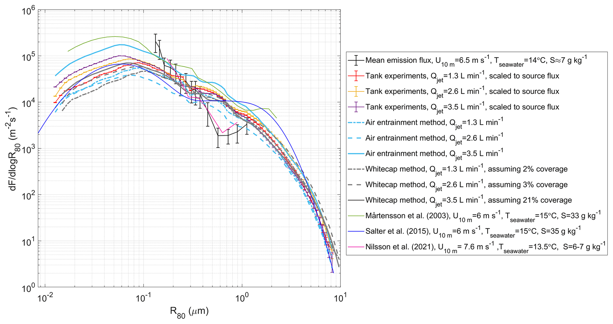
Figure 7Comparison of the mean in situ aerosol emission fluxes measured on the island of Östergarnsholm with simulation chamber measurements that are scaled to the mean emission flux derived from both campaigns, together with the fluxes estimated using the continuous whitecap method and air entrainment measurements. The scaled fluxes from the chamber measurements are presented as a mean with a standard error, while the EC-derived aerosol emission fluxes are presented as a mean with a random error and a discrete counting error. For comparison, EC-derived aerosol fluxes from Nilsson et al. (2021) and SSA parameterizations from Mårtensson et al. (2003) and Salter et al. (2015) are also included.
3.5 Comparison of scaled chamber data and in situ emission fluxes to previous studies
Figure 7 also illustrates the comparison between the scaled chamber fluxes, in situ emission fluxes, and existing sea spray parameterizations by Mårtensson et al. (2003) and Salter et al. (2015) (U10 m=6 m s−1 and C). Both parameterizations show reasonably good agreement with the in situ data, with slightly higher values from the Mårtensson parameterization and slightly lower values from the Salter parameterization. These parameterizations were derived from chamber experiments with artificial seawater at salinities of 33 and 35 g kg−1, respectively. However, Zinke et al. (2022) reported an increase in aerosol particle production at lower salinities (6–8 g kg−1) relevant to the Baltic Sea, where these measurements were conducted, compared to higher salinities (∼ 35 g kg−1). The authors attributed this to an increased number of large bubbles at lower salinities, which tend to produce numerous small film drops. The only previous sea spray aerosol flux measurements from the Baltic Sea were conducted by Nilsson et al. (2021), which show emission fluxes that agree well with the emission fluxes derived from this study.
In their study, Nilsson et al. (2021) attempted to scale co-located chamber experiments to EC flux measurements using the same approach employed in the current study. However, they were unable to derive a scaling factor between the chamber measurements and in situ fluxes due to differences in the slopes of the size distributions resulting from both methods. This discrepancy may have been due to the inclusion of fluxes obtained from sectors with short fetches and shallow waters. The success of the current dataset in this regard is likely attributed to the use of a large, homogeneous dataset that is clearly defined as open sea with a long fetch.
3.6 Wind-speed- and wave-state-dependent parameterizations of the scaled chamber data
In Sect. 3.2.2 and 3.2.3, we discussed the dependence of SSA emission fluxes on both wind speed and wave state. In this section, we have developed parameterizations of the aerosol emission flux as a function of wind speed and wave Reynolds number, which takes into account wave height, friction velocity, and seawater viscosity, which in turn depends on seawater temperature and salinity. Both parameterizations are valid for seawater temperatures between 10 and 20 ∘C and salinities between 6 and 7 g kg−1, which represent large parts of the Baltic Proper during the summer half of the year. We used scaled chamber data that encompass dry particle diameters µm as a basis for the parameterizations. To parameterize the emission flux, we fit the scaled chamber data (binned based on wind speed or wave Reynolds number) to the sum of three log-normal distributions of the form
In the wind-speed-dependent parameterization, the magnitude of each mode is parameterized by a log-linear relationship. For the wave-state-dependent parameterization, we adopted a similar approach to that used by Ovadnevaite et al. (2014). Table 4 provides the modal diameters (Dmod,i), geometric standard deviations (σi), and log-linear relationships for the magnitude EFi for each mode. Figures S17 and S18 illustrate how the derived relationships fit the modes of the scaled chamber data with increasing wind speeds and wave Reynolds number, respectively.
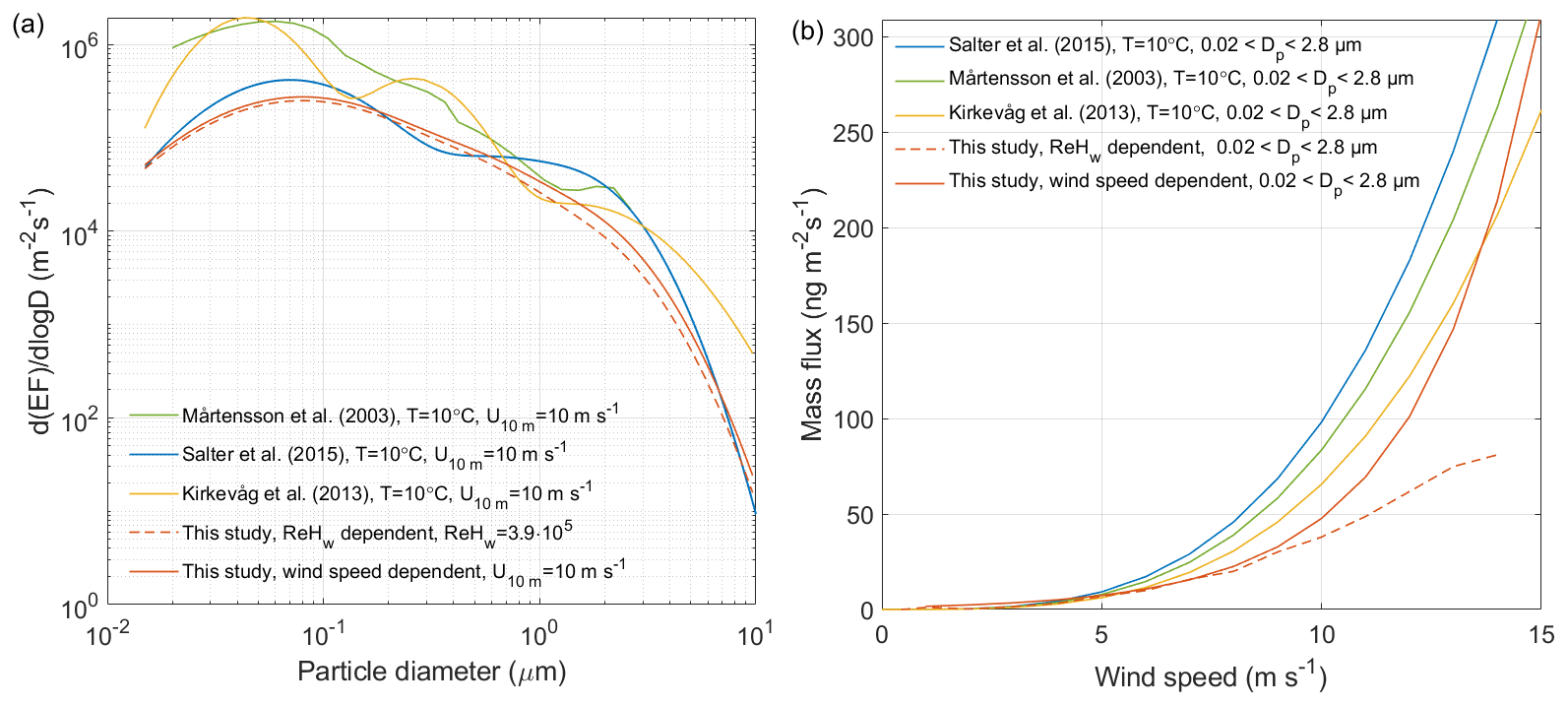
Figure 8Comparison of the wind-speed- and wave-state-dependent parameterizations derived from this study with those from studies, including Mårtensson et al. (2003), Kirkevåg et al. (2013), and Salter et al. (2015). Panel (a) shows emission estimates at U10 m= 10 m s−1, while panel (b) shows the estimated mass emission flux for particles with dry diameters µm, which is the range in which the Mårtensson et al. (2003) parameterization is valid. The wave-state-dependent parameterization is based on averaging the wave Reynolds number within the corresponding wind speed bins and using these mean wave Reynolds number values as the foundation for the parameterization.
Table 4The modal diameters Dmod,i, geometric standard deviations (σi), and log-linear relationships for the number fluxes (EFi) of each of the three log-normal modes in the parameterization derived in this study.
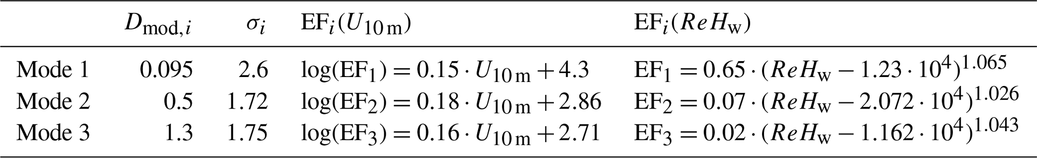
Figure 8 shows that the wind-speed-dependent parameterization derived in this study produces size-resolved number emission fluxes and mass emission estimates that agree well with those obtained from the parameterizations by Mårtensson et al. (2003), Kirkevåg et al. (2013), and Salter et al. (2015). Although recent studies suggest that sea state is a better predictor of SSA emissions than wind speed alone (Norris et al., 2013; Ovadnevaite et al., 2014; Yang et al., 2019), our wave Reynolds number-dependent parameterization yields lower mass emission fluxes than the wind-speed-dependent parameterizations, particularly at wind speeds above 10 m s−1. When compared to the mass estimates from the in situ EC flux measurements over the measured size range (see Fig. S19), these agree very well for wind speeds <7 m s−1 but deviate for higher wind speeds. The parameterizations by Mårtensson et al. (2003), Kirkevåg et al. (2013), and Salter et al. (2015) were developed for high-salinity conditions. Thus, it is reasonable to expect lower mass production in the sea spray simulation chamber at lower salinities (S≈7 g kg−1), such as those encountered in the Baltic Sea (Zinke et al., 2022). To the best of our knowledge, prior studies have not specifically examined the influence of lower salinity on wave-breaking patterns. However, this factor could potentially elucidate some of the disparities observed between our flux estimates and those conducted in higher-salinity waters.
In this study, we compared SSA production fluxes derived from sea spray simulation chamber measurements and in situ EC fluxes measured close to the ICOS station on the island of Östergarnsholm during two ship-based campaigns in May and August 2021. By combining these datasets, we quantified the magnitude and size-resolved spectrum of SSA fluxes using fast EC flux measurements across the full range of particle sizes relevant for SSA emissions. During the two campaigns, we observed a log-linear relationship between the total in situ emission fluxes and wind speed, a power-law relationship between the total emission fluxes and significant wave height, and a linear relationship between the total emission fluxes and wave Reynolds number, similar to what has been reported in several previous studies. In contrast, we did not observe any significant impact of wind speed or dissolved oxygen concentration on the size-resolved particle production in the sea spray simulation chamber experiments, as reported in previous studies. We only observed a weak negative correlation between the particle production and the concentration of chlorophyll α together with a weak positive correlation between the particle production and the concentration of FDOM in the seawater.
We were able to scale the chamber measurements at three different jet flow rates to obtain realistic emission fluxes using three different approaches: (1) the continuous whitecap method, (2) measurements of air entrainment, and (3) scaling the chamber measurements to the in situ emission fluxes. The measured in situ fluxes and scaled chamber data also agreed well with previous flux measurements from the Baltic Sea (Nilsson et al., 2021) and the parameterizations by Mårtensson et al. (2003) and Salter et al. (2015).
Finally, we derived wind-dependent and wave-state-dependent parameterizations of SSA emissions at low salinities representative of the Baltic Proper. The number and mass emission estimates derived from the wind-speed-dependent parameterization are in good agreement with previous studies, while the wave-state-dependent parameterization yields lower mass emission estimates. We attributed this difference to the lower salinity of the Baltic Sea and the fact that the Baltic Sea is a semi-enclosed sea and might not always be representative of open-ocean conditions.
The combination of laboratory experiments and EC measurements in this study is crucial for understanding how well laboratory estimates of SSA emission fluxes represent in situ emission fluxes. This has significant implications for several reasons. Laboratory estimates of SSA emission fluxes cover the entire range of aerosol particle sizes produced by bursting bubbles. However, the accuracy of laboratory systems in replicating the wave-breaking process is still uncertain. Nevertheless, the reasonably good agreement between laboratory emission estimates using the air entrainment scaling and the in situ fluxes suggests that this approach can provide realistic estimates of SSA production. Secondly, certain aerosol types and properties cannot be effectively measured at the high frequencies required for EC measurements. For instance, the EC approach is inadequate for accurately estimating bacteria fluxes from the ocean to the atmosphere. On the other hand, laboratory systems are capable of measuring bacteria fluxes. Therefore, combining laboratory measurements with EC measurements allows us to derive realistic estimates of bacteria flux.
Based on these findings, our future work will involve utilizing multi-year EC measurements to investigate seasonal cycles in SSA emission fluxes from a coastal site in the Baltic Sea. Our focus will be particularly on emissions of bioaerosols contained within SSA. By integrating measurements from both the laboratory sea spray chamber and EC techniques, our aim is to develop a comprehensive understanding of SSA fluxes and the environmental factors influencing them.
A1 Systematic errors
A1.1 Losses in aerosol fluxes due to the limited response time of the OPC
To accurately measure EC fluxes, instruments must have a time resolution of 10–20 Hz to capture the smallest eddies. However, some instruments like OPCs are unable to achieve this resolution, resulting in significant flux attenuation. To correct for this, we used the equations for the atmospheric surface layer from Horst (1997). By solving the integral of transfer functions and co-spectra analytically, they derived the flux attenuation (Fa) as follows:
Here is the ideal flux that would have been measured if the sensor response time was not too long (where NX is either Ni or Ntotal), nm is the dimensionless frequency at the co-spectral maximum and is a function of atmospheric stability, τc is the instrument's first-order response time, and is the mean wind speed at measurement height zm. Here α=1 for stable stratification and for neutral and unstable stratification. The normalized frequency nm can be estimated for stable stratification () as follows:
For neutral and unstable conditions, nm=0.085. The first-order response time τc should be determined experimentally following Buzorius et al. (2001) and Buzorius et al. (2003). Ahlm et al. (2010) determined τc to be 0.3 s for the Grimm 1.109 OPC. This allows us to calculate the systematic error of the limited response time δlrt as
Therefore, the corrected flux is
A1.2 Fluctuation attenuation due to air transport in the tubes of closed-path systems
Attenuation of turbulent fluctuations in the sampling tube causes an underestimation of the EC flux (δasl). Co-spectral power frequency transfer functions can be used to estimate the corresponding loss of particle fluctuations in laminar flow (Lenschow and Raupach, 1991). Following Ahlm et al. (2010) and Horst (1997), we used a first-order response time of 0.4 s to estimate the damping in the sampling lines and the OPC, which will be described in detail in the next section. The aerosol EC fluxes were corrected as follows:
A1.3 Aerosol particle losses within the sampling line
Particle losses due to Brownian diffusion, impaction, interception, and sedimentation in the sampling line were estimated using a program written by Hsieh (1991). Since the OPC mostly measures particles in the accumulation mode, Brownian diffusion was small within the OPC range. The sampling lines were arranged vertically to minimize deposition losses. Therefore, the corrected aerosol flux for each size bin is
where δtpl(i) is the corrected size-dependent tube particle losses, and the corrected total aerosol flux for the entire OPC size range is
A1.4 Webb correction
The Webb correction (Webb et al., 1980), also known as the WPL correction after all three co-authors, is required because fluctuations in temperature and humidity can cause fluctuations in scalar concentrations that are not related to the trace gas flux to be measured. For a scalar X, such as gas or particles, with an average concentration , the Webb correction can be written as
Here, is the ratio of molar masses of dry air and water, is the dry air density, and is the average water vapour concentration or density. We applied this correction to both H2O and CO2 fluxes calculated from the Licor7500, resulting in the corrected fluxes for CO2 and H2O:
Temperature fluctuations in tubing with high thermal conductivity are reduced to 1 % of their initial value when the tubing length-to-diameter ratio was for laminar flow and for turbulent flow (Leuning and Judd, 1996). For our OPC, which has laminar flow, the ratio is approximately 787. Thus, for the OPC, we can simplify the Webb correction equation to
The corrected aerosol number flux or is now
A2 Random errors
A2.1 Discrete counting error of aerosol EC fluxes
The OPC operates by passing air flow through a laser mounted at a 90∘ angle to a photodiode. On the opposite side of the photodiode, there is a copper mirror that produces light reflection for the photodiode. Each size channel of the OPC has been calibrated separately in comparison to a reference instrument. When a particle passes through the laser, it creates a voltage spike in the photodiode. The height of this signal determines the particle size. Instruments like the OPC and CPCs count each particle discretely. For such instruments, a large part of the random errors is related to the discrete nature of the data. The error in the aerosol number concentration is proportional to , where n is the total count per half-hour period, or , where Q=1.2 L min−1 is the sample flow of the OPC and is the sampling period. This is often called the discrete counting error or the square root counting error. When applied to or , the error expression (for either an individual size bin i or the total OPC size range) becomes
where σw is the vertical wind variance (Fairall et al., 1983; Buzorius et al., 2003).
The data from this study are available at the Bolin Centre for Climate Research database at https://doi.org/10.17043/zinke-2023-baltic-emissions-1 (Zinke et al., 2023).
The supplement related to this article is available online at: https://doi.org/10.5194/acp-24-1895-2024-supplement.
EDN, JZ, MES, and PZ designed the experiments. EDN, PM, and EMM maintained the EC flux station. AR and EN prepared the buoy data and Licor data. JZ and PZ carried out the chamber experiments. The data analysis was conducted by JZ with the help of EDN and EMM. JZ, EDN, and MES prepared the manuscript with contributions from all the co-authors.
At least one of the (co-)authors is a member of the editorial board of Atmospheric Chemistry and Physics. The peer-review process was guided by an independent editor, and the authors also have no other competing interests to declare.
Publisher’s note: Copernicus Publications remains neutral with regard to jurisdictional claims made in the text, published maps, institutional affiliations, or any other geographical representation in this paper. While Copernicus Publications makes every effort to include appropriate place names, the final responsibility lies with the authors.
The ICOS station at Östergarnsholm is maintained by Uppsala University and VR. The Institute of Oceanology, at the Polish Academy of Science, enabled us to use their research vessel, Oceania, anchoring the ship near Östergarnsholm for several days to conduct our sea spray simulation experiments aboard the ship, close to the aerosol flux tower at Östergarnsholm. Furthermore, we thank the crew and captain of R/V Oceania and R/V Electra and the technical staff at ACES, Stockholm University, for their support. We are grateful to Marcin Stokowski for sharing the CTD and dissolved oxygen data for the Oceania cruise with us. The wave data were kindly provided by Heidi Pettersson from the Finnish Meteorological Institute (FMI). We also acknowledge the NOAA Air Resources Laboratory (ARL) for providing the HYSPLIT transport and dispersion model and the READY website (https://www.ready.noaa.gov, last access: 15 November 2022) used in this publication.
The CROISSANT project is financed by the Swedish Research Council project 2018-04255. The aerosol flux tower and system were financed initially by FORMAS, project no. 2007-1362, and have since received contributions from several FORMAS and VR projects. This research was also supported by the Polish National Agency for Academic Exchange under the Bekker Program (Decision PPN/BEK/2019/1/00043/DEC/1) and VR under project 2016-05100. The research is also supported financially by the Bolin Climate Centre at Stockholm University and logistically by Uppsala University.
The article processing charges for this open-access publication were covered by Stockholm University.
This paper was edited by Matthias Tesche and reviewed by Mingxi Yang and two anonymous referees.
Abo Riziq, A., Erlick, C., Dinar, E., and Rudich, Y.: Optical properties of absorbing and non-absorbing aerosols retrieved by cavity ring down (CRD) spectroscopy, Atmos. Chem. Phys., 7, 1523–1536, https://doi.org/10.5194/acp-7-1523-2007, 2007. a
Ahlm, L., Krejci, R., Nilsson, E. D., Mårtensson, E. M., Vogt, M., and Artaxo, P.: Emission and dry deposition of accumulation mode particles in the Amazon Basin, Atmos. Chem. Phys., 10, 10237–10253, https://doi.org/10.5194/acp-10-10237-2010, 2010. a, b, c
Alpert, P. A., Kilthau, W. P., Bothe, D. W., Radway, J. C., Aller, J. Y., and Knopf, D. A.: The influence of marine microbial activities on aerosol production: A laboratory mesocosm study, J. Geophys. Res.-Atmos., 120, 8841–8860, 2015. a
Bowyer, P. A., Woolf, D. K., and Monahan, E. C.: Temperature dependence of the charge and aerosol production associated with a breaking wave in a whitecap simulation tank, J. Geophys. Res.-Oceans, 95, 5313–5319, https://doi.org/10.1029/JC095iC04p05313, 1990. a, b, c
Buzorius, G., Rannik, Ü., Mäkelä, J. M., Vesala, T., and Kulmala, M.: Vertical aerosol particle fluxes measured by eddy covariance technique using condensational particle counter, J. Aerosol Sci., 29, 157–171, 1998. a
Buzorius, G., Rannik, Ü., Nilsson, D., and Kulmala, M.: Vertical fluxes and micrometeorology during aerosol particle formation events, Tellus B, 53, 394–405, 2001. a
Buzorius, G., Rannik, Ü., Nilsson, E., Vesala, T., and Kulmala, M.: Analysis of measurement techniques to determine dry deposition velocities of aerosol particles with diameters less than 100 nm, J. Aerosol Sci., 34, 747–764, 2003. a, b
Callaghan, A.: An improved whitecap timescale for sea spray aerosol production flux modeling using the discrete whitecap method, J. Geophys. Res., 118, 9997–10010, https://doi.org/10.1002/jgrd.50768, 2013. a
Ceburnis, D., Rinaldi, M., Ovadnevaite, J., Martucci, G., Giulianelli, L., and O'Dowd, C. D.: Marine submicron aerosol gradients, sources and sinks, Atmos. Chem. Phys., 16, 12425–12439, https://doi.org/10.5194/acp-16-12425-2016, 2016. a
Christiansen, S., Salter, M. E., Gorokhova, E., Nguyen, Q. T., and Bilde, M.: Sea spray aerosol formation: Laboratory results on the role of air entrainment, water temperature, and phytoplankton biomass, Environ. Sci. Technol., 53, 13107–13116, 2019. a
Cipriano, R. J. and Blanchard, D. C.: Bubble and aerosol spectra produced by a laboratory “breaking wave”, J. Geophys. Res.-Oceans, 86, 8085–8092, 1981. a
Clarke, A. D., Owens, S. R., and Zhou, J. C.: An ultrafine sea-salt flux from breaking waves: Implications for cloud condensation nuclei in the remote marine atmosphere, J. Geophys. Res., 111, D06202, https://doi.org/10.1029/2005JD006565, 2006. a
Craig, V. S. J., Ninham, B. W., and Pashley, R. M.: The effect of electrolytes on bubble coalescence in water, J. Phys. Chem., 97, 10192–10197, https://doi.org/10.1021/j100141a047, 1993. a
de Leeuw, G., Andreas, E. L., Anguelova, M. D., Fairall, C. W., Lewis, E. R., O'Dowd, C. D., Schulz, M., and Schwartz, S. E.: Production flux of sea spray aerosol, Rev. Geophys., 49, RG2001, https://doi.org/10.1029/2010RG000349, 2011. a
Dubitsky, L., Stokes, M., Deane, G., and Bird, J.: Effects of salinity beyond coalescence on submicron aerosol distributions, J. Geophys. Res.-Atmos., 128, e2022JD038222, https://doi.org/10.1029/2022JD038222, 2023. a
Facchini, M. C., Rinaldi, M., Decesari, S., Carbone, C., Finessi, E., Mircea, M., Fuzzi, S., Ceburnis, D., Flanagan, R., Nilsson, E. D., de Leeuw, G., Martino, M., Woeltjen, J., and O'Dowd, C. D.: Primary submicron marine aerosol dominated by insoluble organic colloids and aggregates, Geophys. Res. Lett., 35, L17814, https://doi.org/10.1029/2008GL034210, 2008. a, b
Fairall, C. W., Davidson, K. L., and Schaucher, G. E.: An analysis of the surface production of sea-salt aerosol, Tellus B, 35, 31–39, 1983. a
Forestieri, S., Moore, K., Martinez Borrero, R., Wang, A., Stokes, M., and Cappa, C.: Temperature and composition dependence of sea spray aerosol production, Geophys. Res. Lett., 45, 7218–7225, https://doi.org/10.1029/2018GL078193, 2018. a, b, c
Fossum, K. N., Ovadnevaite, J., Ceburnis, D., Preißler, J., Snider, J. R., Huang, R.-J., Zuend, A., and O’Dowd, C.: Sea-spray regulates sulfate cloud droplet activation over oceans, NPJ Clim. Atmos. Sci., 3, 1–6, 2020. a
Fuentes, E., Coe, H., Green, D., de Leeuw, G., and McFiggans, G.: On the impacts of phytoplankton-derived organic matter on the properties of the primary marine aerosol – Part 1: Source fluxes, Atmos. Chem. Phys., 10, 9295–9317, https://doi.org/10.5194/acp-10-9295-2010, 2010. a
Geever, M., O'Dowd, C. D., van Ekeren, S., Flanagan, R., Nilsson, E. D., de Leeuw, G., and Rannik, U.: Submicron sea spray fluxes, J. Geophys. Res., 32, L15810, https://doi.org/10.1029/2005GL023081, 2005. a, b, c, d, e
Gong, S. L.: A parameterization of sea-salt aerosol source function for sub- and super-micron particles, Global Biogeochem. Cy., 17, 1097, https://doi.org/10.1029/2003GB002079, 2003. a
Grythe, H., Ström, J., Krejci, R., Quinn, P., and Stohl, A.: A review of sea-spray aerosol source functions using a large global set of sea salt aerosol concentration measurements, Atmos. Chem. Phys., 14, 1277–1297, https://doi.org/10.5194/acp-14-1277-2014, 2014. a
Gutiérrez-Loza, L., Nilsson, E., Wallin, M. B., Sahlée, E., and Rutgersson, A.: On physical mechanisms enhancing air–sea CO2 exchange, Biogeosciences, 19, 5645–5665, https://doi.org/10.5194/bg-19-5645-2022, 2022. a
Hallgren, C., Arnqvist, J., Nilsson, E., Ivanell, S., Shapkalijevski, M., Thomasson, A., Pettersson, H., and Sahlée, E.: Classification and properties of non-idealized coastal wind profiles – an observational study, Wind Energ. Sci., 7, 1183–1207, https://doi.org/10.5194/wes-7-1183-2022, 2022. a
Haywood, J. M., Ramaswamy, V., and Soden, B. J.: Tropospheric aerosol climate forcing in clear-sky satellite observations over the oceans, Science, 283, 1299–1303, https://doi.org/10.1126/science.283.5406.1299, 1999. a
Högström, U., Sahlée, E., Drennan, W. M., Kahma, K. K., Smedman, A.-S., Johansson, C., Pettersson, H., Rutgersson, A., Tuomi, L., Zhang, F., and Johansson, M.: Momentum fluxes and wind gradients in the marine boundary layer – A multi-platform study, Boreal Environ. Res., 13, 475–502, 2008. a
Horst, T.: A simple formula for attenuation of eddy fluxes measured with first-order-response scalar sensors, Bound.-Lay. Meteorol., 82, 219–233, 1997. a, b, c
Hsieh, K.-C.: Studies of particle reentrainment/detachment from flat surface, University of Minnesota, ISBN 979-8-207-67007-2, 1991. a, b
Hultin, K. A. H., Nilsson, E. D., Krejci, R., Mårtensson, E. M. Ehn, M., Hagström, A., and de Leeuw, G.: In situ laboratory sea spray production during the Marine Aerosol Production 2006 cruise on the northeastern Atlantic Ocean, J. Geophys. Res.-Atmos., 115, D06201, https://doi.org/10.1029/2009JD012522, 2010. a, b, c, d
Hultin, K. A. H., Krejci, R., Pinhassi, J., Gomez-Consarnau, L., Mårtensson, E. M., Hagström, A., and Nilsson, E. D.: Aerosol and bacterial emissions from Baltic seawater, Atmos. Res., 99, 1–14, https://doi.org/10.1016/j.atmosres.2010.08.018, 2011. a, b
Keene, W. C., Maring, H., Maben, J. R., Kieber, D. J., Pszenny, A. A. P., Dahl, E. E., Izaguirre, M. A., Davis, A. J., Long, M. S., Zhou, X., Smoydzin, L., and Sander, R.: Chemical and physical characteristics of nascent aerosols produced by bursting bubbles at a model air–sea interface, J. Geophys. Res., 112, D21202, https://doi.org/10.1029/2007JD008464, 2007. a, b
Kirkevåg, A., Iversen, T., Seland, Ø., Hoose, C., Kristjánsson, J. E., Struthers, H., Ekman, A. M. L., Ghan, S., Griesfeller, J., Nilsson, E. D., and Schulz, M.: Aerosol–climate interactions in the Norwegian Earth System Model – NorESM1-M, Geosci. Model Dev., 6, 207–244, https://doi.org/10.5194/gmd-6-207-2013, 2013. a, b, c, d
Lee, C., Sultana, C. M., Collins, D. B., Santander, M. V., Axson, J. L., Malfatti, F., Cornwell, G. C., Grandquist, J. R., Deane, G. B., Stokes, M. D., and Azam, F.: Advancing model systems for fundamental laboratory studies of sea spray aerosol using the microbial loop, J. Phys. Chem. A, 119, 8860–8870, 2015. a
Lenschow, D. and Raupach, M.: The attenuation of fluctuations in scalar concentrations through sampling tubes, J. Geophys. Res.-Atmos., 96, 15259–15268, 1991. a
Leuning, R. and Judd, M. J.: The relative merits of open-and closed-path analysers for measurement of eddy fluxes, Glob. Change Biol., 2, 241–253, 1996. a
Lewis, E. R. and Schwartz, S. E.: Sea Salt Aerosol Production: Mechanisms, Methods, Measurements and Models – A Critical Review, Geophysical Monograph Series, Vol. 152, American Geophysical Union, ISBN 978-0-875-90417-7, 2004. a, b
Liu, S., Liu, C.-C., Froyd, K. D., Schill, G. P., Murphy, D. M., Bui, T. P., Dean-Day, J. M., Weinzierl, B., Dollner, M., Diskin, G. S., et al.: Sea spray aerosol concentration modulated by sea surface temperature, Proceedings of the National Academy of Sciences, 118, e2020583118, https://doi.org/10.1073/pnas.2020583118, 2021. a
Long, M. S., Keene, W. C., Kieber, D. J., Erickson, D. J., and Maring, H.: A sea-state based source function for size- and composition-resolved marine aerosol production, Atmos. Chem. Phys., 11, 1203–1216, https://doi.org/10.5194/acp-11-1203-2011, 2011. a, b, c, d, e
Mårtensson, E. M., Nilsson, E. D., de Leeuw, G., Cohen, L. H., and Hansson, H. C.: Laboratory simulations and parameterization of the primary marine aerosol production, J. Geophys. Res.-Atmos., 108, 4297, https://doi.org/10.1029/2002JD002263, 2003. a, b, c, d, e, f, g, h, i, j, k, l, m, n, o, p
Markuszewski, P., Klusek, Z., Nilsson, E. D., and Petelski, T.: Observations on relations between marine aerosol fluxes and surface-generated noise in the southern Baltic Sea, Oceanologia, 62, 413–427, 2020. a
Mårtensson, E. M., Nilsson, E. D., Buzorius, G., and Johansson, C.: Eddy covariance measurements and parameterisation of traffic related particle emissions in an urban environment, Atmos. Chem. Phys., 6, 769–785, https://doi.org/10.5194/acp-6-769-2006, 2006. a
Massey Jr., F. J.: The Kolmogorov-Smirnov test for goodness of fit, J. Am. Stat. Assoc., 46, 68–78, https://doi.org/10.1080/01621459.1951.10500769, 1951. a
May, N. W., Axson, J. L., Watson, A., Pratt, K. A., and Ault, A. P.: Lake spray aerosol generation: a method for producing representative particles from freshwater wave breaking, Atmos. Meas. Tech., 9, 4311–4325, https://doi.org/10.5194/amt-9-4311-2016, 2016. a, b
Modini, R., Russell, L., Deane, G., and Stokes, M.: Effect of soluble surfactant on bubble persistence and bubble-produced aerosol particles, J. Geophys. Res.-Atmos., 118, 1388–1400, 2013. a, b
Monahan, E., Wang, Q., Wang, X., and Wilson, M.: Air entrainment by breaking waves: A laboratory assessment, ASME-Publications-FED, 187, p. 21, 1994. a
Monahan, E. C. and O'Muircheartaigh, I.: Optimal power-law description of oceanic whitecap coverage dependence on wind speed, J. Phys. Oceanogr., 10, 2094–2099, https://doi.org/10.1175/1520-0485(1980)010<2094:OPLDOO>2.0.CO;2, 1980. a, b, c, d
Monahan, E. C., Spiel, D. E., and Davidson, K. L.: Whitecap aerosol productivity deduced from simulation tank measurements, J. Geophys. Res., 87, 8898–8904, 1982. a, b
Monahan, E. C., Fairall, C. W., Davidson, K. L., and Boyle, P. C.: Observed inter-relations between 10m winds, ocean white caps and marine aerosols, Q. J. Roy. Meteor. Soc., 109, 379–392, 1983. a
Monahan, E. C., Spiel, D. E., and Davidson, K. L.: Oceanic Whitecaps, chap. A model of marine aerosol generation via whitecaps and wave disruption, D. Reidel Publishing Company, 167–174, https://doi.org/10.1007/978-94-009-4668-2_16, 1986. a
Murphy, D., Anderson, J., Quinn, P., McInnes, L., Brechtel, F., Kreidenweis, S., Middlebrook, A., Pósfai, M., Thomson, D., and Buseck, P.: Influence of sea-salt on aerosol radiative properties in the Southern Ocean marine boundary layer, Nature, 392, 62–65, https://doi.org/10.1038/32138, 1998. a
Nielsen, L. S. and Bilde, M.: Exploring controlling factors for sea spray aerosol production: temperature, inorganic ions and organic surfactants, Tellus B, 72, 1–10, https://doi.org/10.1080/16000889.2020.1801305, 2020. a, b, c
Nilsson, E. D., Rannik, U., Swietlicki, E., Leck, C., Aalto, P. P., Zhou, J., and Norman, M.: Turbulent aerosol fluxes over the Arctic Ocean: 2. Wind-driven sources from the sea, J. Geophys. Res., 106, 32139–32154, https://doi.org/10.1029/2000JD900747, 2001. a, b, c, d, e, f
Nilsson, E. D., Hultin, K. A., Mårtensson, E. M., Markuszewski, P., Rosman, K., and Krejci, R.: Baltic Sea Spray Emissions: In Situ Eddy Covariance Fluxes vs. Simulated Tank Sea Spray, Atmosphere, 12, 274, https://doi.org/10.3390/atmos12020274, 2021. a, b, c, d, e, f, g, h, i, j, k, l, m, n, o, p
Norris, S. J., Brooks, I. M., de Leeuw, G., Smith, M. H., Moerman, M., and Lingard, J. J. N.: Eddy covariance measurements of sea spray particles over the Atlantic Ocean, Atmos. Chem. Phys., 8, 555–563, https://doi.org/10.5194/acp-8-555-2008, 2008. a, b, c, d
Norris, S. J., Brooks, I. M., Hill, M. K., Brooks, B. J., Smith, M. H., and Sproson, D. A. J.: Eddy covariance measurements of the sea spray aerosol flux over the open ocean, J. Geophys. Res.-Atmos., 117, D07210, https://doi.org/10.1029/2011JD016549, 2012. a, b, c
Norris, S. J., Brooks, I. M., and Salisbury, D. J.: A wave roughness Reynolds number parameterization of the sea spray source flux, Geophys. Res. Lett., 40, 4415–4419, 2013. a, b, c
Ovadnevaite, J., Manders, A., de Leeuw, G., Ceburnis, D., Monahan, C., Partanen, A.-I., Korhonen, H., and O'Dowd, C. D.: A sea spray aerosol flux parameterization encapsulating wave state, Atmos. Chem. Phys., 14, 1837–1852, https://doi.org/10.5194/acp-14-1837-2014, 2014. a, b, c, d, e, f, g, h, i
Park, J. Y., Lim, S., and Park, K.: Mixing state of submicrometer sea spray particles enriched by insoluble species in bubble-bursting experiments, J. Atmos. Ocean. Tech., 31, 93–104, https://doi.org/10.1175/JTECH-D-13-00086.1, 2014. a, b
Prather, K. A., Bertram, T. H., Grassian, V. H., Deane, G. B., Stokes, M. D., DeMott, P. J., Aluwihare, L. I., Palenik, B. P., Azam, F., Seinfeld, J. H., and Moffet, R. C.: Bringing the ocean into the laboratory to probe the chemical complexity of sea spray aerosol, P. Natl. Acad. Sci. USA, 110, 7550–7555, 2013. a
Quinn, P., Coffman, D., Kapustin, V., Bates, T., and Covert, D.: Aerosol optical properties in the marine boundary layer during the First Aerosol Characterization Experiment (ACE 1) and the underlying chemical and physical aerosol properties, J. Geophys. Res.-Atmos., 103, 16547–16563, https://doi.org/10.1029/97JD02345, 1998. a
Quinn, P. K., Bates, T. S., Schulz, K. S., Coffman, D. J., Frossard, A. A., Russell, L. M., Keene, W. C., and Kieber, D. J.: Contribution of sea surface carbon pool to organic matter enrichment in sea spray aerosol, Nat. Geosci., 7, 228–232, https://doi.org/10.1038/NGEO2092, 2014. a
Rolph, G., Stein, A., and Stunder, B.: Real-time environmental applications and display system: READY, Environ. Model. Softw., 95, 210–228, 2017. a
Russell, L. M. and Singh, E. G.: Submicron Salt Particle Production in Bubble Bursting, Aerosol Sci. Tech., 40, 664–671, https://doi.org/10.1080/02786820600793951, 2006. a, b
Rutgersson, A., Pettersson, H., Nilsson, E., Bergström, H., Wallin, M. B., Nilsson, E. D., Sahlée, E., Wu, L., and Mårtensson, E. M.: Using land-based stations for air–sea interaction studies, Tellus A, 72, 1–23, 2020. a, b, c, d, e, f
Salter, M. E., Nilsson, E. D., Butcher, A., and Merete, B.: On the seawater temperature dependence of continuous plunging jet derived sea spray aerosol, J. Geophys. Res.-Atmos., 119, 9052–9072, https://doi.org/10.1002/2013JD021376, 2014. a, b, c, d, e
Salter, M. E., Zieger, P., Acosta Navarro, J. C., Grythe, H., Kirkevåg, A., Rosati, B., Riipinen, I., and Nilsson, E. D.: An empirically derived inorganic sea spray source function incorporating sea surface temperature, Atmos. Chem. Phys., 15, 11047–11066, https://doi.org/10.5194/acp-15-11047-2015, 2015. a, b, c, d, e, f, g, h, i, j, k, l, m, n, o
Schack Jr., C. J., Pratsinis, S. E., and Friedlander, S.: A general correlation for deposition of suspended particles from turbulent gases to completely rough surfaces, Atmos. Environ., 19, 953–960, 1985. a
Schwartz, S. E.: The whitehouse effect – Shortwave radiative forcing of climate by anthropogenic aerosols: An overview, J. Aerosol Sci., 27, 359–382, https://doi.org/10.1016/0021-8502(95)00533-1, 1996. a
Schwier, A. N., Sellegri, K., Mas, S., Charrière, B., Pey, J., Rose, C., Temime-Roussel, B., Jaffrezo, J.-L., Parin, D., Picard, D., Ribeiro, M., Roberts, G., Sempéré, R., Marchand, N., and D'Anna, B.: Primary marine aerosol physical flux and chemical composition during a nutrient enrichment experiment in mesocosms in the Mediterranean Sea, Atmos. Chem. Phys., 17, 14645–14660, https://doi.org/10.5194/acp-17-14645-2017, 2017. a, b, c
Sellegri, K., O'Dowd, C. D., Yoon, Y. J., Jennings, S. G., and de Leeuw, G.: Surfactants and submicron sea spray generation, J. Geophys. Res., 111, D22215, https://doi.org/10.1029/2005JD006658, 2006. a, b, c
Slauenwhite, D. E. and Johnson, B. D.: Bubble shattering: Differences in bubble formation in fresh water and seawater, J. Geophys. Res.-Oceans, 104, 3265–3275, https://doi.org/10.1029/1998JC900064, 1999. a
Smedman, A., Högström, U., Bergström, H., Rutgersson, A., Kahma, K., and Pettersson, H.: A case study of air-sea interaction during swell conditions, J. Geophys. Res.-Oceans, 104, 25833–25851, 1999. a
Spiel, D. E.: A hypothesis concerning the peak in film drop production as a function of bubble size, J. Geophys. Res., 102, 1153–1161, https://doi.org/10.1029/96JC03069, 1997. a
Stein, A., Draxler, R. R., Rolph, G. D., Stunder, B. J., Cohen, M., and Ngan, F.: NOAA’s HYSPLIT atmospheric transport and dispersion modeling system, B. Am. Meteorol. Soc., 96, 2059–2077, 2015. a
Svensson, N., Bergström, H., Sahlée, E., and Rutgersson, A.: Stable atmospheric conditions over the Baltic Sea: model evaluation and climatology, Boreal Environ. Res., 21, 387–404, 2016. a
Tyree, C. A., Hellion, V. M., Alexandrova, O. A., and Allen, J. O.: Foam droplets generated from natural and artificial seawaters, J. Geophys. Res.-Atmos., 112, D12204, https://doi.org/10.1029/2006JD007729, 2007. a, b, c, d
von der Weiden, S.-L., Drewnick, F., and Borrmann, S.: Particle Loss Calculator – a new software tool for the assessment of the performance of aerosol inlet systems, Atmos. Meas. Tech., 2, 479–494, https://doi.org/10.5194/amt-2-479-2009, 2009. a
Wang, X., Sultana, C. M., Trueblood, J., Hill, T. C., Malfatti, F., Lee, C., Laskina, O., Moore, K. A., Beall, C. M., McCluskey, C. S., and Cornwell, G. C.: Microbial control of sea spray aerosol composition: A tale of two blooms, ACS Central Science, 1, 124–131, https://doi.org/10.1021/acscentsci.5b00148, 2015. a
Webb, E. K., Pearman, G. I., and Leuning, R.: Correction of flux measurements for density effects due to heat and water vapour transfer, Q. J. Roy. Meteor. Soc., 106, 85–100, 1980. a, b
Wolf, A. and Laca, E. A.: Cospectral analysis of high frequency signal loss in eddy covariance measurements, Atmos. Chem. Phys. Discuss., 7, 13151–13173, https://doi.org/10.5194/acpd-7-13151-2007, 2007. a
Woodcock, A. H.: Salt nuclei in marine air as a function of altitude and wind force, J. Meteor., 10, 362–371, 1953. a
Woolf, D. K., Bowyer, P. A., and Monahan, E. C.: Discriminating between the film drops and jet drops produced by a simulated whitecap, J. Geophys. Res.-Oceans, 92, 5142–5150, https://doi.org/10.1029/JC092iC05p05142, 1987. a, b, c
Yang, M., Prytherch, J., Kozlova, E., Yelland, M. J., Parenkat Mony, D., and Bell, T. G.: Comparison of two closed-path cavity-based spectrometers for measuring air–water CO2 and CH4 fluxes by eddy covariance, Atmos. Meas. Tech., 9, 5509–5522, https://doi.org/10.5194/amt-9-5509-2016, 2016. a
Yang, M., Norris, S. J., Bell, T. G., and Brooks, I. M.: Sea spray fluxes from the southwest coast of the United Kingdom – dependence on wind speed and wave height, Atmos. Chem. Phys., 19, 15271–15284, https://doi.org/10.5194/acp-19-15271-2019, 2019. a, b, c, d, e, f, g, h, i, j, k, l, m
Zábori, J., Matisāns, M., Krejci, R., Nilsson, E. D., and Ström, J.: Artificial primary marine aerosol production: a laboratory study with varying water temperature, salinity, and succinic acid concentration, Atmos. Chem. Phys., 12, 10709–10724, https://doi.org/10.5194/acp-12-10709-2012, 2012. a, b, c, d, e
Zábori, J., Krejci, R., Ström, J., Vaattovaara, P., Ekman, A. M. L., Salter, M. E., Mårtensson, E. M., and Nilsson, E. D.: Comparison between summertime and wintertime Arctic Ocean primary marine aerosol properties, Atmos. Chem. Phys., 13, 4783–4799, https://doi.org/10.5194/acp-13-4783-2013, 2013. a
Zhao, D. and Toba, Y.: Dependence of whitecap coverage on wind and wind-wave properties, J. Oceanogr., 57, 603–616, 2001. a
Zieger, P., Väisänen, O., Corbin, J. C., Partridge, D. G., Bastelberger, S., Mousavi-Fard, M., Rosati, B., Gysel, M., Krieger, U. K., Leck, C., and Nenes, A.: Revising the hygroscopicity of inorganic sea salt particles, Nat. Commun., 8, 1–10, https://doi.org/10.1038/ncomms15883, 2017. a
Zinke, J., Nilsson, E. D., Zieger, P., and Salter, M. E.: The Effect of Seawater Salinity and Seawater Temperature on Sea Salt Aerosol Production, J. Geophys. Res.-Atmos., 127, e2021JD036005, https://doi.org/10.1029/2021JD036005, 2022. a, b, c, d, e, f
Zinke, J., Nilsson, E., Markuszewski, P., Zieger, P., Mårtensson, E., Rutgersson, A., Nilsson, E., and Salter, M.: Comparison of aerosol eddy covariance fluxes and chamber-simulated sea spray emissions from the Baltic Sea, Bolin Centre for Climate Research [data set], https://doi.org/10.17043/zinke-2023-baltic-emissions-1, 2023. a
- Abstract
- Introduction
- Measurement site and methods
- Results and discussion
- Summary and conclusion
- Appendix A: Loss estimates and systematic error corrections
- Data availability
- Author contributions
- Competing interests
- Disclaimer
- Acknowledgements
- Financial support
- Review statement
- References
- Supplement