Cloud properties and their projected changes in CMIP models with low to high climate sensitivity

Since the release of the first Coupled Model Intercomparison Project version 6 (CMIP6) simulations, one of the most discussed topics is the higher effective climate sensitivity (ECS) of some of the models, resulting in an increased range of ECS values in CMIP6 compared to previous CMIP phases. An important contribution to ECS is the cloud climate feedback. Although climate models have continuously been developed and improved over the last few decades, a realistic representation of clouds remains challenging. Clouds contribute to the large uncertainties in modeled ECS, as projected changes in cloud properties and cloud feedbacks also depend on the simulated present-day fields.

In this study, we investigate the representation of both cloud physical and radiative properties from a total of 51 CMIP5 and CMIP6 models. ECS is used as a simple metric to group the models, as the sensitivity of the physical cloud properties to warming is closely related to cloud feedbacks, which in turn are known to have a large contribution to ECS. Projected changes in the cloud properties in future scenario simulations are analyzed by the ECS group. In order to help with interpreting the projected changes, model results from historical simulations are also analyzed.

The results show that differences in the net cloud radiative effect as a reaction to warming among the three model groups are driven by changes in a range of cloud regimes rather than individual regions. In polar regions, high-ECS models show a weaker increase in the net cooling effect of clouds, due to warming, than the low-ECS models. At the same time, high-ECS models show a decrease in the net cooling effect of clouds over the tropical ocean and the subtropical stratocumulus regions, whereas low-ECS models show either little change or even an increase in the cooling effect. Over the Southern Ocean, the low-ECS models show a higher sensitivity of the net cloud radiative effect to warming than the high-ECS models.

1 Introduction

Climate models are an essential tool for projecting future climate. Within the context of the Coupled Model Intercomparison Project (CMIP, https://www.wcrp-climate.org/wgcm-cmip, last access: 29 January 2024), a World Climate Research Programme (WCRP) initiative, several modeling groups worldwide provide a set of coordinated simulations with different Earth system models (ESMs) of the past (historical) time period and different future scenarios. The main objective of CMIP is to better understand past, present, and future climate, its variability, and future change arising from both natural, unforced variability and in response to changes in radiative forcing in a multi-model context.

Across the different CMIP phases, several improvements, e.g., in the climatological large-scale patterns of temperature, water vapor, and zonal wind speed were found, with the latest phase models (CMIP6, Eyring et al., 2016) typically performing slightly better than their CMIP3 and CMIP5 predecessors when compared to observations (Bock et al., 2020). While this is also the case for some cloud properties and selected regions such as the Southern Ocean, clouds remain challenging for global climate models, with many known biases remaining in CMIP6 (Lauer et al., 2023). As such, clouds continue to play a significant role in uncertainties in the climate models and climate projections (Bony et al., 2015).

One of the extensively discussed topics in the analyses of the CMIP6 ensemble is the higher effective climate sensitivity (ECS) of some models and therefore the increased range in ECS, which is now between 1.8 and 5.6 K compared to 2.1 and 4.7 K in the CMIP5 ensemble (Meehl et al., 2020; Bock et al., 2020; Schlund et al., 2020). ECS provides a single number, defined as the change in global mean near-surface air temperature, resulting from a doubling of the atmospheric CO₂ concentration compared to preindustrial conditions, once the climate has reached a new equilibrium (Gregory et al., 2004). A possible reason for the increase in the ECS in some models is improvements in cloud representation in these models. Zelinka et al. (2020) show that the increased range of ECS in the CMIP6 models could be explained by an increased range in cloud feedbacks. Studies using single models concluded that the increased climate sensitivity found in these models is largely determined by cloud microphysical processes (Zhu et al., 2022; Frey and Kay, 2018; Gettelman et al., 2019; Bodas‐Salcedo et al., 2019). They also point out that the simulated present-day mean state of cloud properties is related to the simulated cloud feedback but could also be connected to other coupled feedbacks (Andrews et al., 2019).

As future changes in cloud properties are closely connected to cloud feedbacks, and cloud feedbacks are known to be strongly correlated with ECS (see Sect. 3.1), we use ECS as a simple proxy to group the ensemble of CMIP5 and CMIP6 models for this analysis. This facilitates the analysis and allows for obtaining more general conclusions beyond individual models that can vary widely in their sensitivity to the prescribed forcings. A particular focus of this study is whether there are systematic differences in cloud-related quantities between the different ECS groups. The sensitivity of the physical properties to warming is analyzed, as this gives some insight into the uncertainty in the projected cloud properties and their potential contribution to cloud feedbacks and ECS.

A comparison of the present-day climatologies of key cloud properties from the different ECS model groups is done to help interpreting simulated future changes in cloud properties. The present-day performance of CMIP models has been investigated, for example, by Kuma et al. (2023), who applied an artificial neural network to derive cloud types from radiation fields. They found that results from models with a high ECS agree on average better with observations than with those from models with a low ECS. Jiang et al. (2021) found that the models' ECS is positively correlated with the integrated cloud water content and water vapor performance scores for both CMIP6 and CMIP5 models. In contrast, Brunner et al. (2020) showed that some CMIP6 models with a high future warming compared to other models receive systematically lower-performance weights when using the anomaly, variance, and trend of surface air temperature and anomaly and variance of sea level pressure to assess the models' performance.

A number of different feedbacks is relevant to ECS, with cloud feedbacks being an important contribution. In order to assess whether there are systematic differences in simulated cloud properties among models with different ECS, we compare the simulated cloud properties from three groups of models sorted by their ECS values and quantify how the projected changes in cloud properties and cloud radiative effects differ. In Sect. 2, we briefly introduce the models and observations used, as well as the software tool applied to compare the models. The representation of cloud radiative effects for all three groups is also compared with observational data in Sect. 3, followed by an analysis of the projected future changes in cloud properties and radiative effects. Section 4 summarizes the discussion and conclusions.

2 Data

2.1 Models

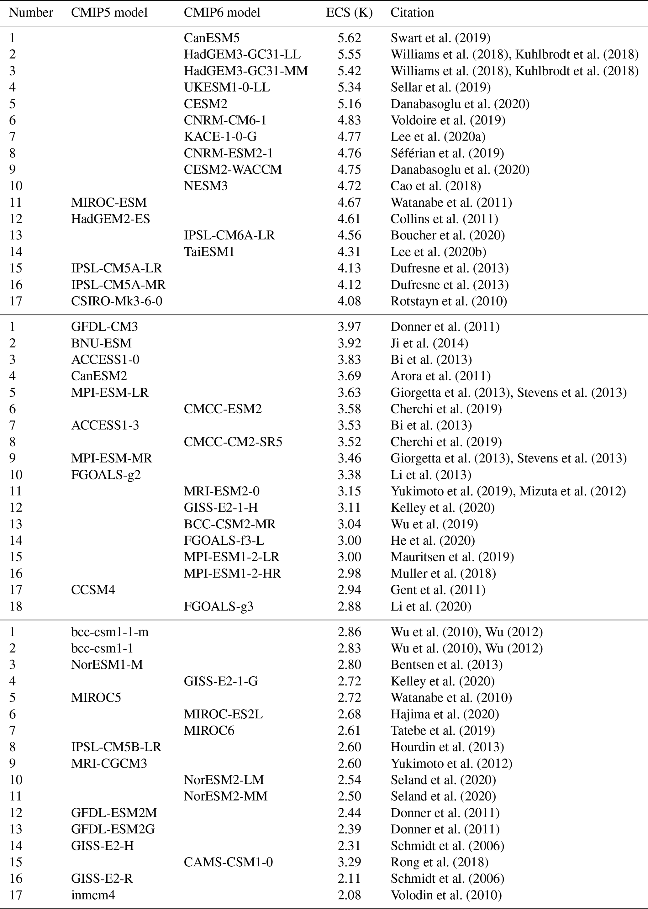
In this study, we use model simulations from the CMIP Phases 5 (Taylor et al., 2012) and 6 (Eyring et al., 2016). The individual models are detailed in Table 1. All model data are freely available via the Earth System Grid Federation (ESGF), which is an international collaboration that manages the decentralized database of CMIP output.

Swart et al. (2019)Williams et al. (2018)Kuhlbrodt et al. (2018)Williams et al. (2018)Kuhlbrodt et al. (2018)Sellar et al. (2019)Danabasoglu et al. (2020)Voldoire et al. (2019)Lee et al. (2020a)Séférian et al. (2019)Danabasoglu et al. (2020)Cao et al. (2018)Watanabe et al. (2011)Collins et al. (2011)Boucher et al. (2020)Lee et al. (2020b)Dufresne et al. (2013)Dufresne et al. (2013)Rotstayn et al. (2010)Donner et al. (2011)Ji et al. (2014)Bi et al. (2013)Arora et al. (2011)Giorgetta et al. (2013)Stevens et al. (2013)Cherchi et al. (2019)Bi et al. (2013)Cherchi et al. (2019)Giorgetta et al. (2013)Stevens et al. (2013)Li et al. (2013)Yukimoto et al. (2019)Mizuta et al. (2012)Kelley et al. (2020)Wu et al. (2019)He et al. (2020)Mauritsen et al. (2019)Muller et al. (2018)Gent et al. (2011)Li et al. (2020)Wu et al. (2010)Wu (2012)Wu et al. (2010)Wu (2012)Bentsen et al. (2013)Kelley et al. (2020)Watanabe et al. (2010)Hajima et al. (2020)Tatebe et al. (2019)Hourdin et al. (2013)Yukimoto et al. (2012)Seland et al. (2020)Seland et al. (2020)Donner et al. (2011)Donner et al. (2011)Schmidt et al. (2006)Rong et al. (2018)Schmidt et al. (2006)Volodin et al. (2010)

Table 1 List of CMIP5 and CMIP6 models grouped by ECS value into three roughly equally sized groups, namely high (ECS > 4.0 K), medium (2.87 K < ECS < 4.0 K), and low (ECS < 2.87 K).

For the analysis presented here, we use historical simulations over the time period from 1985–2004 (Table 1) and the scenario simulations of the Representative Concentration Pathway (RCP) 8.5 from CMIP5 and the Shared Socioeconomic Pathway (SSP) 5–8.5 simulations from CMIP6 for the years 2081–2100. The historical simulations use prescribed natural and anthropogenic climate forcings such as concentrations of greenhouse gases and aerosols. We only consider one ensemble member per model, typically the first member, i.e., r1i1p1 (CMIP5) and r1i1p1f1 (CMIP6). As the intermodel spread is typically much larger than the interensemble spread, we do not expect our results to change significantly when using more ensemble members for each model. For further details on the model simulations, we refer to Taylor et al. (2012) and Eyring et al. (2016).

ECS and cloud feedbacks are calculated using the simulations forced by an abrupt quadrupling of CO₂ (abrupt-4× CO₂) and the preindustrial control simulations (piControl), following the method described in Andrews et al. (2012) and Schlund et al. (2020).

In total, the CMIP ensemble investigated here consists of 24 CMIP5 and 27 CMIP6 models that provide the output needed for this analysis. We grouped them into the three groups, low, medium, and high, by their ECS values (see Table 1). The thresholds for the three groups are chosen in a way such that each of the three groups contains the same number of models. Multi-model group means are calculated as 20-year means over all models in the high-, medium-, and low-ECS group, applying equal weights to each model.

2.2 Observations

The Clouds and the Earth's Radiant Energy System (CERES) Energy Balanced and Filled (EBAF) Ed4.2 dataset (Loeb et al., 2018; Kato et al., 2018) provides global monthly mean top-of-atmosphere (TOA) longwave (LW), shortwave (SW), and net radiative fluxes under clear-sky and all-sky conditions, which are used as a reference dataset to calculate the cloud radiative effects and the TOA outgoing radiation. CERES instruments are on board NASA's Terra and Aqua satellites.

The dataset covers whole years for the time period 2001–2022. We would like to note that the time period from the models used for comparison with the CERES–EBAF dataset (Sect. 2.1) does not exactly match the observed years. ESMs are not expected to reproduce the exact observed phase of climate modes, which largely control present-day variability in the clouds but rather their statistical properties. Therefore, it is probably not surprising that this difference in the time periods has very little impact on the multiyear group averages when comparing multi-year climatologies of cloud parameters.

Starting with CERES–EBAF Ed4.1, the dataset provides adjusted clear-sky fluxes, which are now defined in a manner that is more in line with how clear-sky fluxes are represented in climate models. The uncertainty estimates for 1${}^{\circ }\times {\mathrm{1}}^{\circ }$ regional monthly net cloud radiative effects are about 7 W m⁻² (CERES-EBAF, 2021).

2.3 ESMValTool

All analyses in this study are performed with the open-source community diagnostics and performance metrics tool for evaluation of ESMs called the Earth System Model Evaluation Tool (ESMValTool) version 2 (Eyring et al., 2020; Lauer et al., 2020; Righi et al., 2020; Weigel et al., 2021; Schlund et al., 2023). All figures from this paper can be reproduced by running the ESMValTool “recipe” tool (with a configuration script defining all datasets, processing steps, and diagnostics), recipe_bock24acp.yml (see also the “Code and data availability” section).

3 Analysis

3.1 ECS and cloud feedback

The large spread in ECS of CMIP6 models could mainly be explained by uncertainties in the simulated net cloud feedback. The net cloud feedback is defined as change in the sum of shortwave and longwave cloud radiative effects at the TOA per degree of surface warming (2 m temperature), which is calculated as the difference between abrupt-4× CO₂ simulations and the corresponding piControl simulations. The TOA shortwave and longwave cloud radiative effects are calculated as the differences between the respective TOA all-sky and clear-sky radiative fluxes. While this method is commonly used to calculated cloud feedbacks, we would like to note that the results using this method are not exactly the same as those calculated with a more accurate offline radiative transfer method (Soden et al., 2004). Particularly the shortwave cloud radiative effect can be affected in regions with high surface albedos, such as polar latitudes, if the surface albedo changes between the two model simulations, e.g., because of melting sea ice (Shell et al., 2008). The net cloud feedback is typically dominated by the shortwave component (Zelinka et al., 2020).

The relation between ECS and simulated cloud feedbacks is illustrated in Fig. 1, which shows the correlation between net, shortwave, and longwave cloud feedbacks and ECS in the CMIP5 and CMIP6 models (Table 1). The relation between net cloud feedback and ECS is dominated by the shortwave cloud feedback, which shows a strong correlation with ECS (r=0.66 and a small p value of $p=\mathrm{3.6}\times {\mathrm{10}}^{-\mathrm{9}}$). For the longwave cloud feedback, there is only a weak (negative) correlation with ECS (p=0.05).

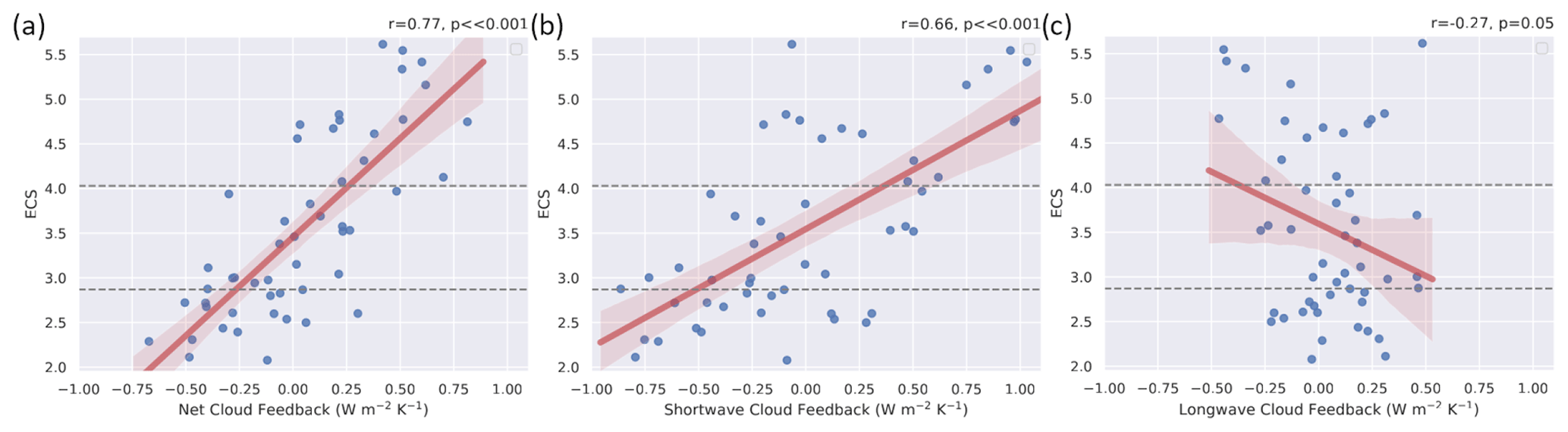
Figure 1 Scatterplot of the global mean (a) net, (b) shortwave, and (c) longwave cloud feedback (x axis) and ECS (y axis) of the CMIP models (Table 1), with a regression line, including the confidence interval of the regression of 95 %. Dashed horizontal lines indicate separations of the three ECS groups (see Table 1).

As the representation of clouds and their sensitivity to climate change have a strong impact on the ECS (Zelinka et al., 2020; Bjordal et al., 2020; Bony et al., 2015) and because the range of ECS obtained from the ensemble of CMIP6 models is larger than the one from the previous model generations (Meehl et al., 2020), this motivated us to look into the differences in present-day performance and future projections of physical cloud parameters from models with low/medium/high ECS.

Figure 2 shows the geographical distributions of the net, shortwave, and longwave cloud feedbacks averaged over all models within each group. The pattern of the net cloud feedback is dominated by the geographical distribution of the shortwave cloud feedback. On global average, the high-ECS group has the largest net cloud feedback of 0.41 W m⁻², followed by the medium-ECS group (0.01 W m⁻²) and the low-ECS group (−0.20 W m⁻²). The group mean net cloud feedback changes sign at around 60^∘ S and 80^∘ N in all three groups. The sign change at around 60^∘ S in the shortwave cloud feedback corresponds to the latitude region, where a change from clouds with an ice component in the piControl simulations to clouds consisting almost entirely of liquid droplets in the abrupt-4× CO₂ experiment (cloud phase feedback) starts to contribute significantly to the total cloud feedback (Ceppi et al., 2017). With increasing latitude, there is an increasing ice fraction in the model clouds that supports a negative shortwave feedback as cloud particles can change phase with warming. Particularly over the Arctic and the tropical Pacific, the (negative) shortwave cloud feedback is partly or fully compensated by a (positive) longwave cloud feedback, resulting in rather small net cloud feedback values.

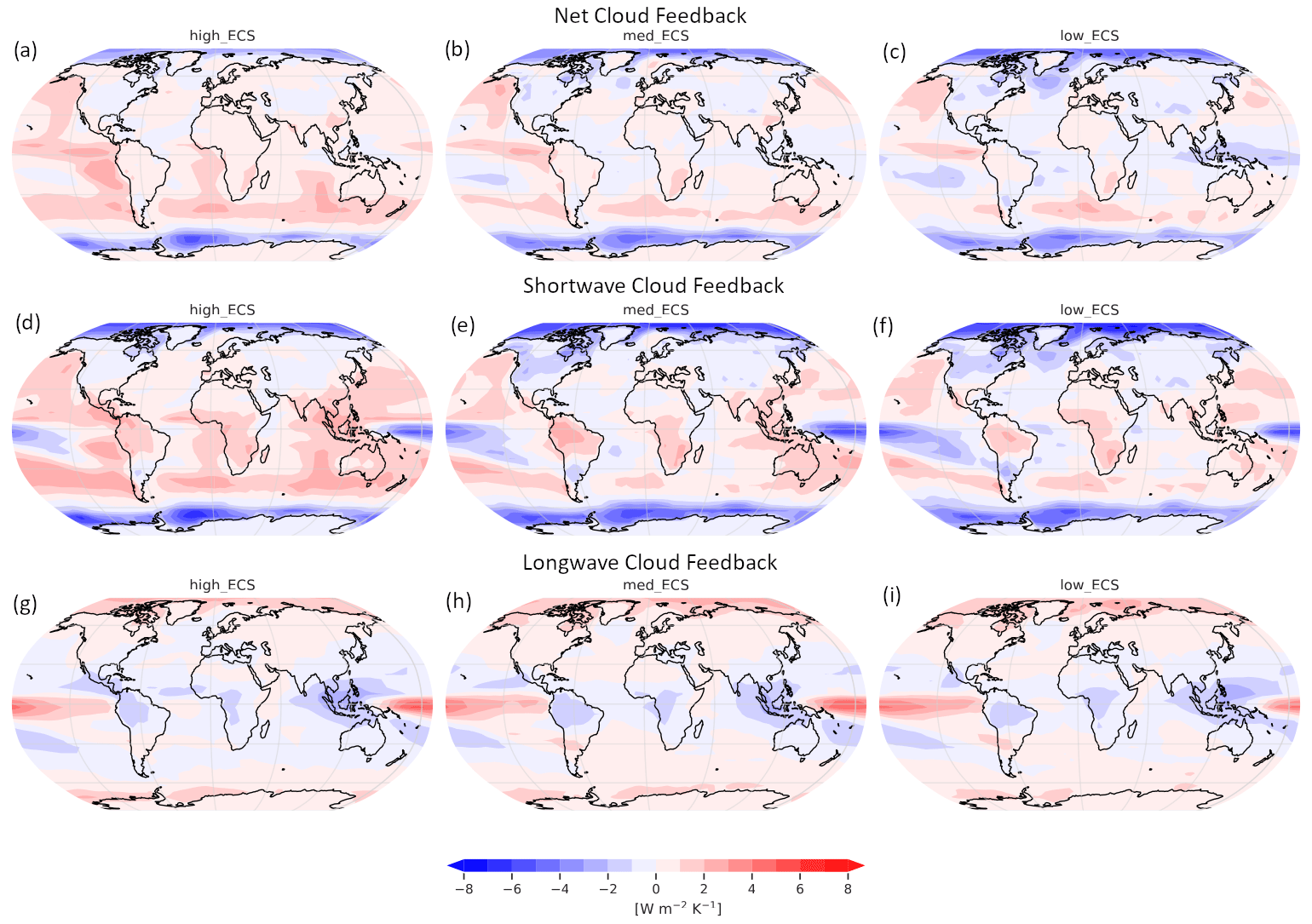
Figure 2 Geographical maps of net (a, b, c), shortwave (d, e, f), and longwave (g, h, i) cloud feedback for high- (left), medium- (middle), and low-ECS (right) groups.

The high-ECS models show a more positive net cloud feedback in the tropics and midlatitudes, especially over the Southern Ocean, than the other two groups. The group mean of the low-ECS models shows a distinct negative net cloud feedback in the tropics, particularly in the tropical Pacific. This signal is much weaker in the other two groups. The reason is a more pronounced negative shortwave cloud feedback particularly over the Pacific Intertropical Convergence Zone (ITCZ) and South Pacific Convergence Zone (SPCZ) in the group mean of the low-ECS models.

3.2 Present-day cloud fields

The representation of cloud properties in ESMs is related to the simulated cloud feedback (Zelinka et al., 2020, 2022). In order to help with interpreting the differences in simulated future changes in cloud properties due to warming among the three ECS groups, we compare the geographical distributions of the climatologies from the individual groups with each other. Here, we focus on the most climate-relevant parameters, which are total cloud fraction, liquid water and ice water path (Fig. 3), and longwave, shortwave, and net cloud radiative effects (Fig. 4). For a direct comparison with satellite observations, output of cloud-related quantities from satellite simulators would be needed. Such output is, however, only available in a very limited form, or not at all, from the models. Comparisons of the model results with observations are therefore restricted to cloud radiative effects for which data are available that could be compared directly with climate model results without using satellite simulators or other sampling strategies (Loeb and Staff, 2022) (see Sect. 2.2 for more details on CERES–EBAF).

Total cloud fraction

The annual mean total cloud fraction from all ECS groups (Fig. 3a–c) shows the known geographical patterns, namely maxima over land in the tropics, due to strong convection; minima in the subtropics because of descending air, with local maxima in stratocumulus regions off the west coasts of the continents (Africa, North America, and South America); maxima in the midlatitudes over the ocean, especially over the Southern Ocean; and minima over polar regions where the air is very cold and dry.

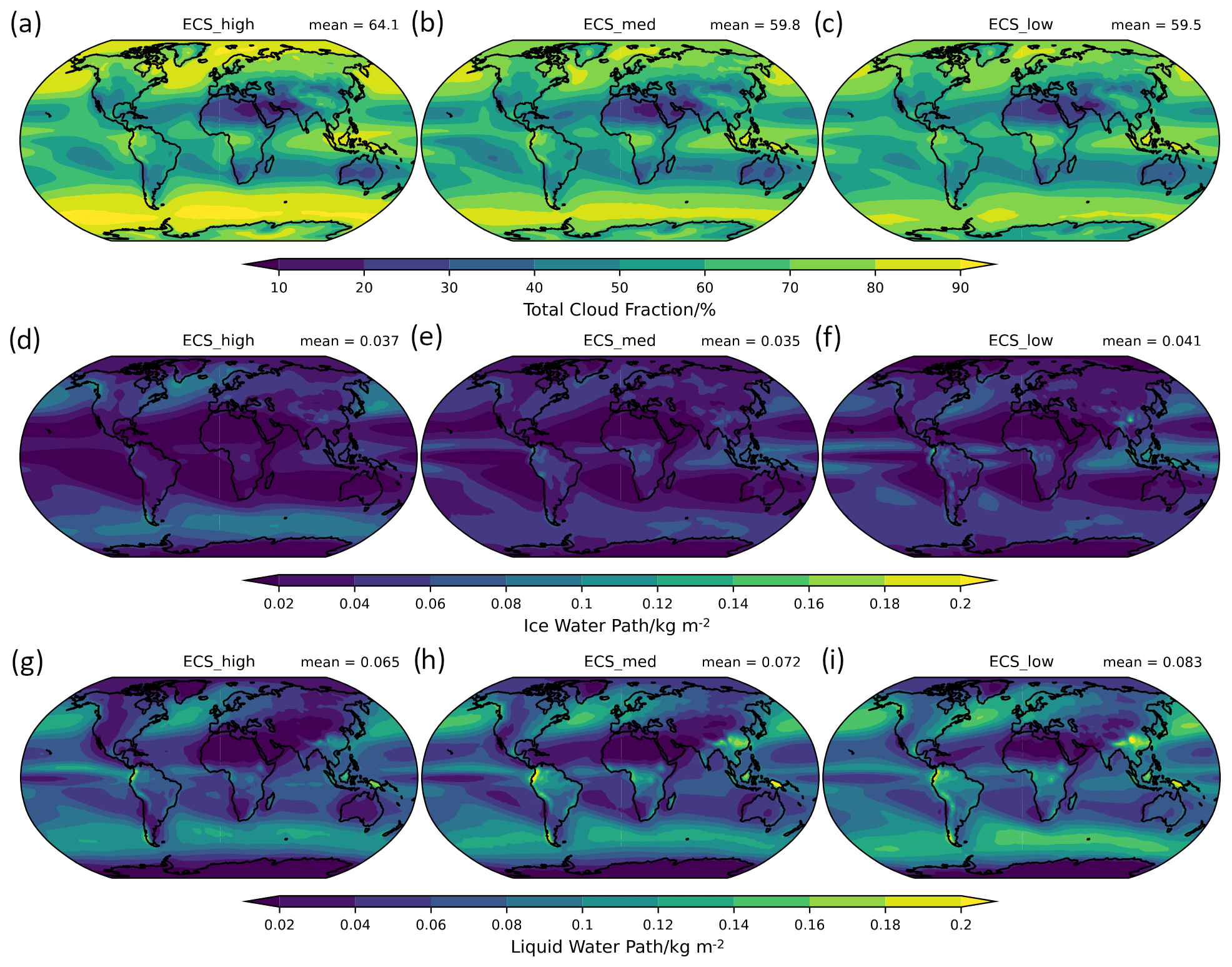
Figure 3 Geographical map of the multi-year annual mean total cloud fraction (a–c), ice water path (d–f), and liquid water path (g–i) for group means of historical CMIP simulations from all three ECS groups.

The group mean of the high-ECS models (Fig. 3a) shows the largest global mean of 64.1 % in total cloud cover compared to 59.8 % and 59.5 % for the medium- and low-ECS groups, respectively. Compared with the intermodel spread given by the quantiles (see Table 2), this difference is a robust signal. The maxima in total cloud cover over the Southern Ocean and the northern Atlantic and Pacific (Fig. 3a) are especially more pronounced (differences up to 10 %) in the group mean of the high-ECS group, which leads to a slight reduction in the known bias of total cloud cover from CMIP models when compared with the CMIP5/6 multi-model mean (Lauer et al., 2023). The minima polewards of about 75^∘ are more pronounced in the low- and medium-ECS models (Fig. 3b, c).

Table 2 Mean values of each group, together with the 25 % and 75 % quantiles (in parentheses), calculated by bootstrapping (1000 times; sample size is the number of models in the group). The second line gives the 25 % and 75 % quantiles calculated from all individual models.

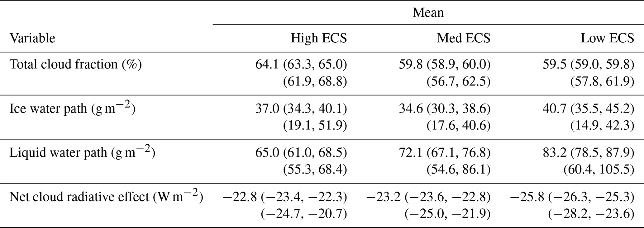
Ice water path

The global distribution of the ice water path (Fig. 3d–f) from all ECS group means shows the maximum in the ITCZ due to frequent convection of up to 0.16 kg m⁻². The absolute minima of the ice water path are found in the subtropics in the subsidence regions west of continents. High amounts of cloud ice are also found along the storm tracks in the midlatitudes, with values decreasing towards the poles.

The intermodel spread in the global mean ice water path (Table 2) is large, resulting in a large overlap between the different ECS groups and no statistically significant difference in the global mean ice water path from the three ECS groups. There are, however, some differences in regional features of the ice water path distribution. The maximum of the ice water path values in the tropics related to the ITCZ are highest in the low-ECS group. In contrast, the maxima in midlatitudes, especially over the Southern Ocean, are most pronounced in the high-ECS models (Fig. 3d).

Liquid water path

The ECS group means of the cloud liquid water path (Fig. 3g–i) show local maxima in the ITCZ, but the largest values of liquid water path are found in the extratropics in the storm track regions, mainly over the Southern Ocean and the northern Atlantic. There are no local maxima in the stratocumulus regions seen in all three group means, which is related to a known bias of underestimating stratocumulus clouds in the CMIP models (e.g., Jian et al., 2020). In addition to the higher cloud cover in the high-ECS group in these regions, the clouds seem to be less bright in comparison to the two other groups. This indicates an improvement of the representation of stratocumulus clouds in the high-ECS group, which is consistent with the findings of Cesana et al. (2023).

The high-ECS group mean shows the lowest global mean (65.0 g m⁻²), followed by the medium-ECS group and the low-ECS group, with 72.1 and 83.2 g m⁻², respectively. This negative correlation between the group-averaged global mean liquid water path and ECS seems quite robust with regard to the relatively small intermodel spread in these two variables within each group. The relative differences between the ECS groups are uniformly distributed, with no region being particularly pronounced.

Cloud radiative effects

The cloud radiative effects are calculated as the differences in TOA clear-sky and all-sky radiative fluxes (for details, see Sect. 3.1). The CERES–EBAF data show a global mean net cooling due to clouds of about −18 W m⁻² (Fig. 4a). Clouds have a warming radiative effect, particularly over regions with a high surface albedo like ice-covered regions in Greenland and Antarctica and the desert regions in North Africa. A large negative (cooling) net radiative effect of clouds is found over the stratocumulus regions in the subtropics and in the midlatitude storm track regions. In the ITCZ, there is a partly compensating effect between the shortwave and longwave radiative effects, leading to smaller absolute net values than in the stratocumulus and storm track regions.

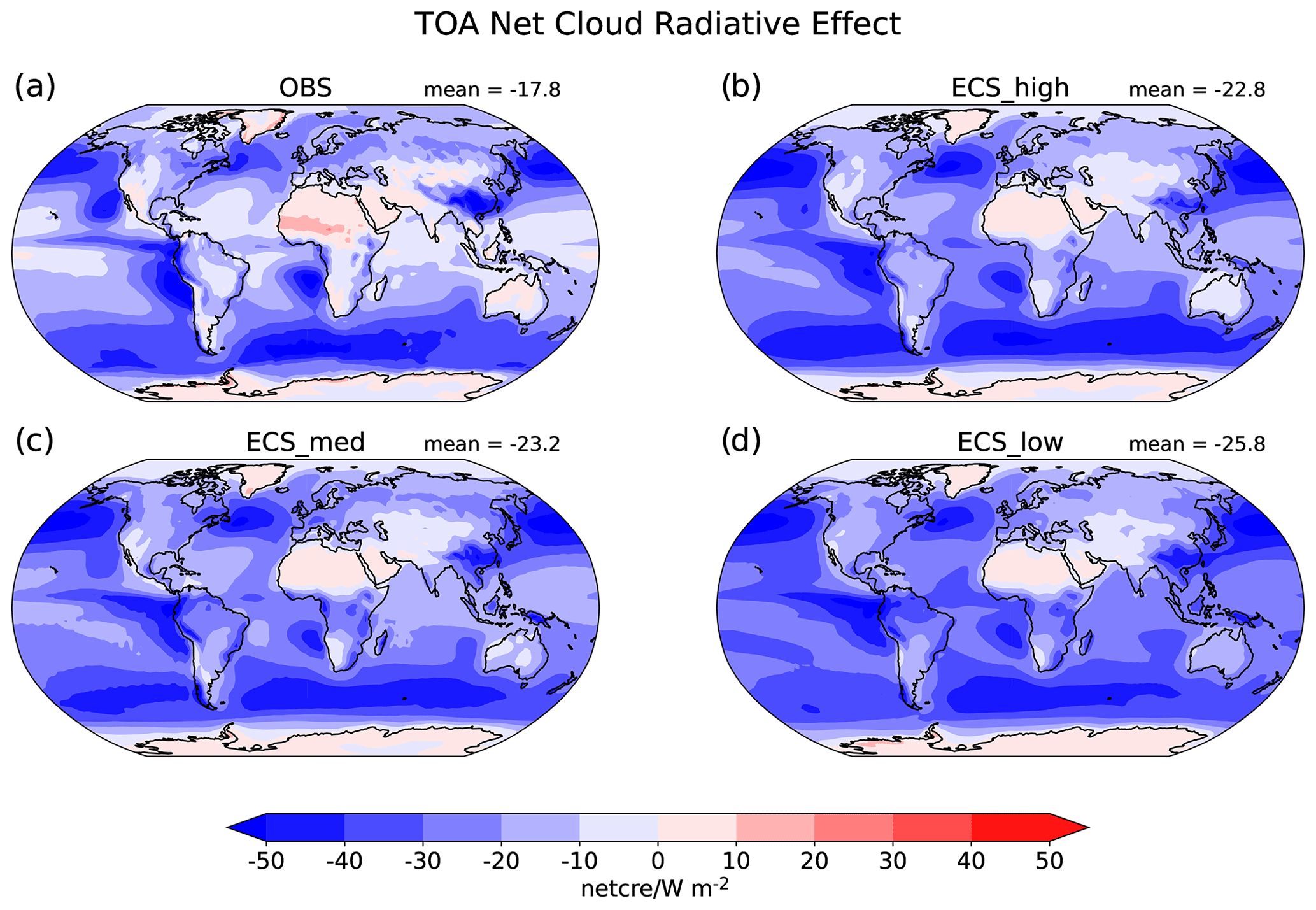
Figure 4 Geographical map of the multi-year annual mean net cloud radiative effect from (a) CERES–EBAF Ed4.2 (OBS) and (b–d) group means of historical CMIP simulations from all three ECS groups.

Table 3 Root mean square difference (RMSD) and pattern correlation of each group mean, together with the 25 % and 75 % quantiles (in parentheses) calculated by bootstrapping (1000 times; sample size is the number of models in the group). The second line gives the 25 % and 75 % quantiles calculated from all individual models. The RMSD values and the correlation are calculated in comparison to the corresponding reference dataset CERES–EBAF (see Sect. 2.2).

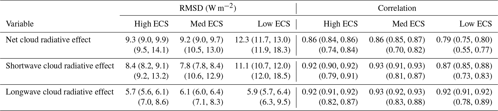
Compared with CERES–EBAF, the amplitude of the global mean net cloud radiative effect is slightly overestimated in the models, with the largest bias in the low-ECS group (mean bias $=-\mathrm{4.8}$ W m⁻²; RMSD =12.3 W m⁻²) and the smallest bias in the high-ECS group (mean bias $=-\mathrm{1.8}$ W m⁻²; RMSD =9.3 W m⁻²) (see also Table 3). While the global mean biases of the group means are within the observational uncertainty range, the RMSD values are larger than the ones of different individual observational datasets when compared to a reference dataset consisting of an average over different products (Lauer et al., 2023).

Biases in simulated sea surface temperatures (SSTs) can affect simulated cloud properties. We therefore also analyzed some results from Atmospheric Model Intercomparison Project (AMIP) simulations that use the atmosphere components of the CMIP models and for which SSTs and sea ice concentrations from observations are prescribed (not shown). Similar to previous studies (e.g., Lauer and Hamilton, 2013; Lauer et al., 2023), we found rather small differences in the multi-year climatologies of cloud properties from the models between the historical and AMIP runs analyzed here. For the net cloud radiative effect, differences between the annual mean climatologies from the historical and AMIP simulations are below 5 W m⁻² throughout most of the globe, but differences in the ITCZ and tropical Atlantic can reach up to about 10 W m⁻². When globally averaged, the mean bias for the average of the three groups ranges between 0.3 and 0.6 W m⁻², RMSE between 2.7 and 3.3 W m⁻², and pattern correlations between 0.97 and 0.98.

The geographical patterns of the three model groups agree well with the CERES–EBAF observations (Fig. 4). The linear pattern correlations of the annual average net cloud radiative effect from the high- and the medium-ECS group means with observations are slightly higher (0.86) than that of the low-ECS (0.79) group. This is also reflected in the range of correlation values from the individual models in each group given by the 25 % and 75 % quantiles. This range lies between 0.55 and 0.77 in the low-ECS group, between 0.70 and 0.82 in the medium-ECS group, and between 0.74 and 0.84 in the high-ECS group. For comparison, the range of correlation coefficients of different observational datasets is 0.98–0.99 (Lauer et al., 2023). The correlation values of the shortwave and longwave cloud radiative effects are larger for all ECS groups.

The peaks of positive cloud forcing over land over Greenland, North Africa, and the west coasts of North America and South America are underestimated in all three groups. In these regions, however, observational uncertainties are expected to be large because of high surface albedo, topography, or very low cloud cover. The largest positive bias for all groups is found over the stratocumulus regions, with up to 46 W m⁻² locally. Apart from this, the low-ECS group shows particularly between 30^∘ S and 30^∘ N (Fig. 4d), which is a net cloud radiative effect that is too strong and results mainly from a shortwave cooling of the clouds in this latitude belt that is too strong (Fig. 6e) and seemingly caused by the largest cloud water path values of all three ECS groups (Fig. 6b, c).

3.3 Differences in projected future cloud properties

In order to investigate the sensitivity of cloud parameters simulated by the three ECS groups to future warming, we compare the changes in selected cloud properties and cloud radiative effects in future simulations from each group. For CMIP6, we calculate the changes as differences between data from SSP5–8.5 and for CMIP5 from RCP8.5 and the results for the respective historical simulations.

The zonally averaged group means (Fig. 6a–f; upper panels of each subfigure) show the results from the historical and the scenario simulations for the investigated cloud properties (total cloud fraction, ice and liquid water path, and cloud radiative effects) for the different ECS groups. Projected zonal mean changes per degree warming (near-surface temperature increase) are displayed in the bottom panels of each subfigure (Fig. 6a–f; lower panels). Additionally, we show the sensitivity of cloud parameters from each ECS group over the ocean for selected regions. The relative changes (calculated as the differences between the scenario value and the historical value divided by the historical value) in cloud parameters per degree warming averaged over selected regions (Fig. 5) are shown in Fig. 7: (1) Arctic, (2) Southern Ocean, (3) tropical ocean, (4) Pacific ITCZ, and the stratocumulus regions of the (5a) southeast Pacific, (5b) southeast Atlantic, and (5c) northeast Pacific.

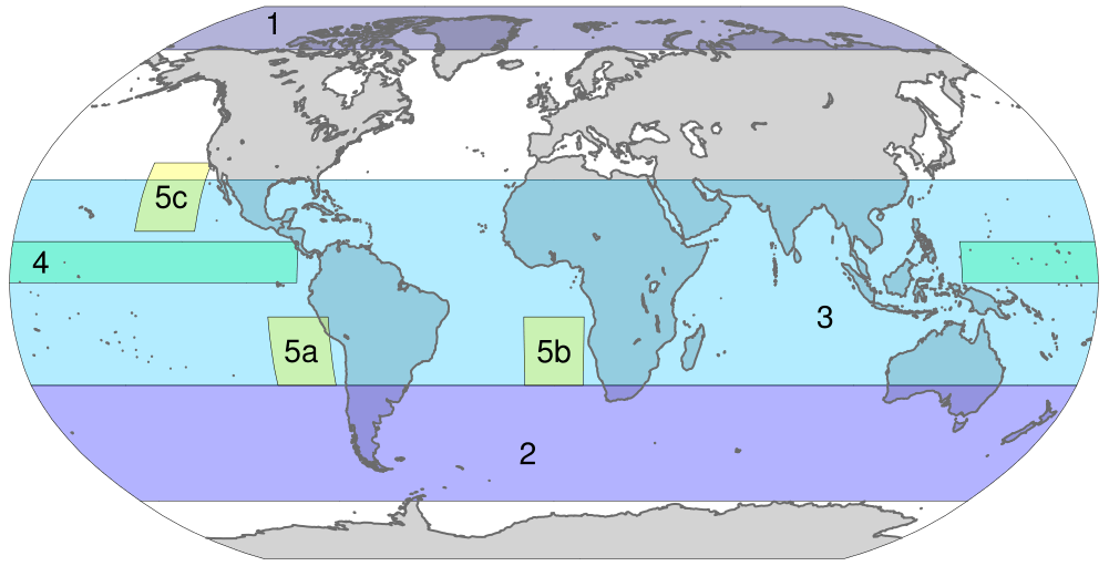
Figure 5 Maps of selected regions. (1) Arctic (70–90^∘ N), (2) Southern Ocean (30–65^∘ S), (3) tropical ocean (30^∘ N–30^∘ S), (4) Pacific ITCZ (0–12^∘ N, 135^∘ E–85^∘ W), and the three stratocumulus regions of the (5a) southeast Pacific (10–30^∘ S, 75–95^∘ W), (5b) southeast Atlantic (10–30^∘ S, 10^∘ W–10^∘ E), and (5c) northeast Pacific (15–35^∘ N, 120–140^∘ W).

In the following, we discuss the differences in projected future cloud properties for each cloud parameter.

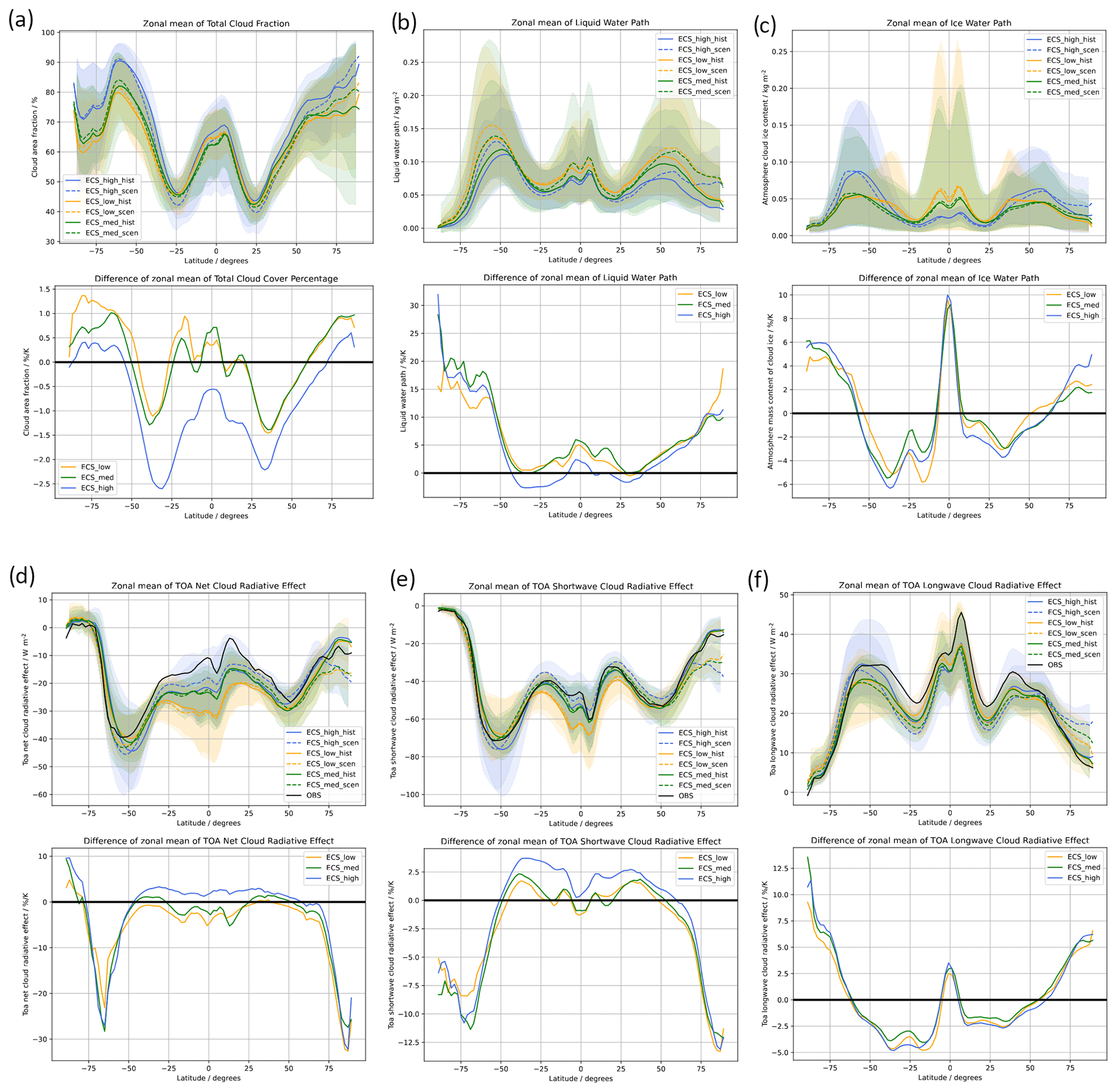
Figure 6 Each labelled subfigure contains two panels, namely the upper panels and lower panels. Upper panels show the zonally averaged group means of (a) total cloud fraction, (b) liquid water path, (c) ice water path, and (d) net, (e) shortwave, and (f) longwave cloud radiative effect from historical simulations (solid lines) and RCP8.5/SSP5-8.5 scenarios (dashed lines) for the three different ECS groups. The reference dataset CERES–EBAF Ed4.2 is shown as solid black lines in panels (d)–(f). Lower panels show the corresponding relative differences of all zonally averaged group means between the RCP8.5/SSP5-8.5 scenarios and the corresponding historical simulations. Shading indicates the 5 % and 95 % quantiles of the single model results.

Total cloud cover

For zonal mean cloud cover (Fig. 6a), the comparison of the historical runs with the scenario simulations shows an increase in the zonal mean cloud cover in particular over the polar regions north and south of about 70^∘. This positive sensitivity to warming shows maximum values ranging between about 0.5 % K⁻¹ for the high-, about 1 % K⁻¹ for the medium-, and 1.4 % K⁻¹ for the low-ECS groups.

Particularly in the tropics and in Southern Hemisphere (SH) mid- and high latitudes, the sensitivity of simulated cloud cover to warming is quite different among the high-ECS group and the two other groups. While the low- and medium-ECS groups show a mostly positive sensitivity in the tropics, the high-ECS group shows a negative sensitivity of cloud cover to warming of about 0.5 to −1.5 % K⁻¹. Averaged over the tropical ocean (Fig. 7c), the behavior of the high-ECS models is significantly different to that of the two other groups. All high-ECS models show a decrease in total cloud cover over the tropical ocean, while the individual models in the two other groups do not agree on the sign of the change.

In all three subtropical stratocumulus regions investigated (northeast Pacific, southeast Pacific, and southeast Atlantic), the high-ECS group shows a decrease in total cloud cover (Fig. 7e). In contrast, the low- and medium-ECS groups show, particularly in the Southern Hemisphere stratocumulus regions, an increase in total cloud cover that is most pronounced in the low-ECS group.

In general, there is a decrease in cloud fraction in midlatitudes which is most pronounced in the high-ECS group and becomes weaker towards the poles. In SH mid- and high latitudes south of 45^∘ S, the low-ECS group shows a strong positive sensitivity of up to more than 1 % K⁻¹, while the high-ECS group shows a negative sensitivity of about −1 % K⁻¹ at 45^∘ S. South of 55^∘ S, the high-ECS group also shows a positive sensitivity of total cloud cover. The medium-ECS group lies in between the low- and high-ECS groups but is in general closer to the low-ECS group. Averaged over the Southern Ocean (latitude belt 30–65^∘ S), the high-ECS models mostly show a negative sensitivity, while the individual models in the two other groups show positive and negative sensitivities.

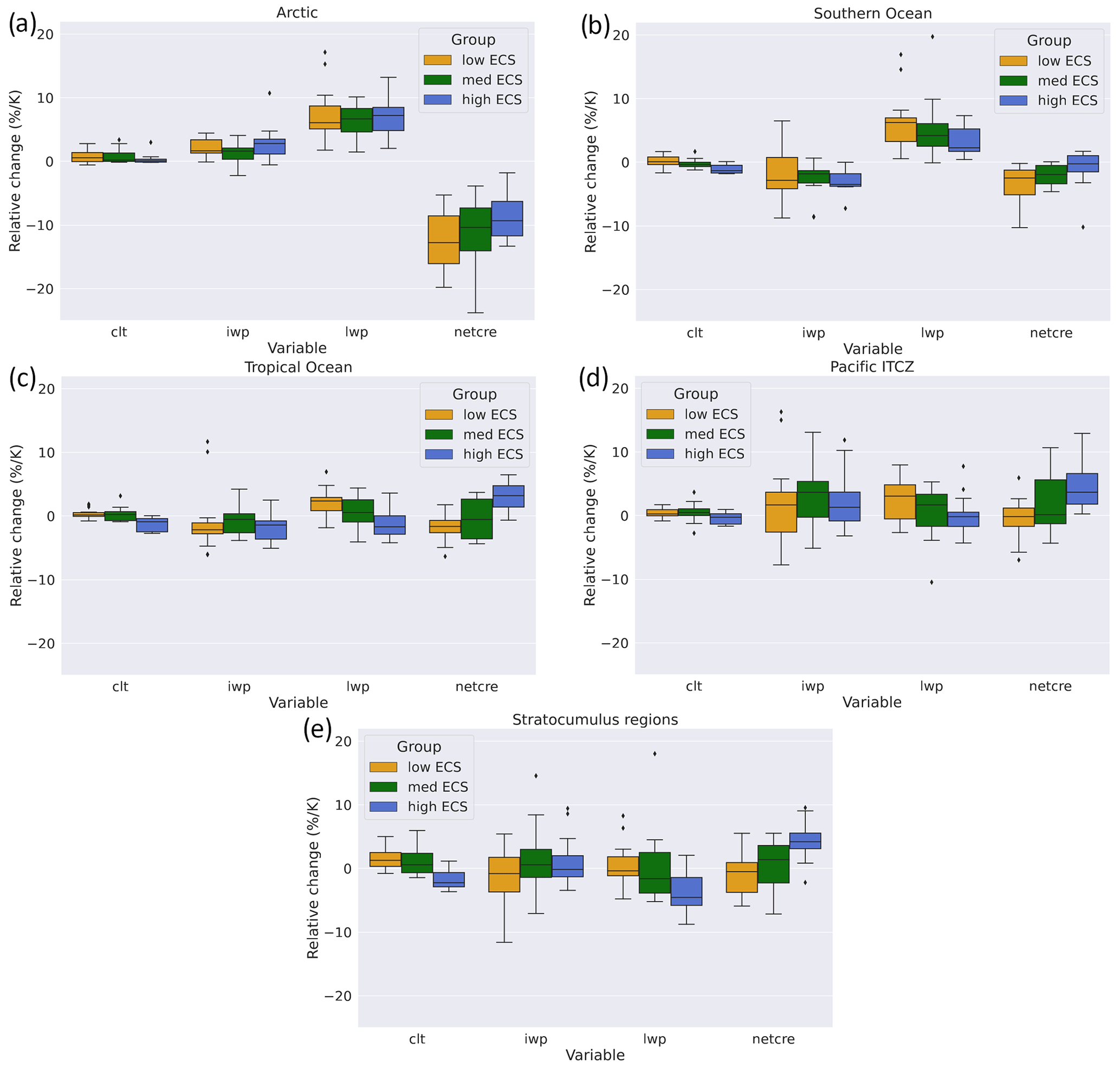
Figure 7 Relative change (calculated as the difference between the scenario value and the historical value divided by the historical value) of total cloud fraction (clt), ice water path (iwp), liquid water path (lwp), and net cloud radiative effect (netcre) per degree of warming averaged over selected regions over the ocean. (a) Arctic (70–90^∘ N), (b) Southern Ocean (30–65^∘ S), (c) tropical ocean (30^∘ N–30^∘ S), (d) Pacific ITCZ (0–12^∘ N, 135^∘ E–85^∘ W), and (e) the three stratocumulus regions of the southeast Pacific (10–30^∘ S, 75–95^∘ W), southeast Atlantic (10–30^∘ S, 10^∘ W–10^∘ E), and northeast Pacific (15–35^∘ N, 120–140^∘ W) (see also Fig. 5). In the box plot, each box indicates the range from the first quartile to the third quartile, the vertical line shows the median, and the whiskers the minimum and maximum values, excluding the outliers. Outliers are defined as being outside 1.5 times the interquartile range.

Cloud liquid and ice water path

In the tropics between about 10^∘ S and 10^∘ N, the cloud ice water path shows a strong sensitivity to warming of up to 9 % K⁻¹ and 10 % K⁻¹ in all three ECS groups (Fig. 6b). The zonally averaged ice water path increases also in all three groups north and south of about 60^∘ N and S, with the high-ECS group showing the strongest sensitivity to warming. Particularly in the Arctic north of 80^∘ N, the sensitivity of the simulated ice water path to warming is about twice as high in the high-ECS group (∼4 % K⁻¹) than in the medium- and low-ECS groups (∼2 % K⁻¹). In midlatitudes, all groups show a negative sensitivity to warming, with the high-ECS group typically showing the strongest sensitivity in the Northern Hemisphere among the three ECS groups.

Similar to the ice water path, the zonally averaged liquid water path also increases with temperature in all three groups in the polar regions (Fig. 6c). This is consistent with the findings of Lelli et al. (2023), who report an observed trend to brighter and more liquid clouds in satellite measurements over the Arctic. In contrast to the ice water path, the lowest ECS group shows the highest sensitivity in the Arctic latitude belt. Averaged over the whole Arctic, however, there are no significant differences in ice and liquid water path over the ocean between the different ECS groups (Fig. 7a).

The amplitude of the decrease in ice water path per degree warming is peaking at about 35^∘ S and N and is about twice as large in the Southern Hemisphere compared to the Northern Hemisphere. Beyond about 60^∘ N and S, there is an increase in the ice water path that is becoming more pronounced towards the poles. This increase in ice water path with warming is even stronger for the liquid water path, with no significant differences between the ECS groups. This increase in the liquid water path can be partly explained by a phase change from cloud ice to liquid at higher temperatures.

In the stratocumulus regions (Fig. 7e), the liquid water path increases in the low-ECS model group, while it decreases in the high-ECS group. The medium-ECS group lies in between the two, with many of the individual models disagreeing on the sign of the change. This behavior is consistent with the sensitivity of the changes in total cloud cover in these regions. We would like to note that ice water path values are typically very small in the stratocumulus regions. Relative changes can therefore be large without being physically relevant.

Over the Southern Ocean, the decrease in ice water path and the increase in liquid water path with warming is also not statistically significantly different among the three ECS groups. Averaged over the whole Southern Ocean (Fig. 7b), all high-ECS models show a decrease in cloud ice water path, whereas about half of the low-ECS models show an increase.

Cloud radiative effects

Over the northern polar region, the cooling effect of the net cloud radiative effect increases significantly for all three ECS groups (Fig. 6d, e, f). Averaged over the whole Arctic (Fig. 7a), the low-ECS group shows the strongest increase in cooling among the three ECS groups. The increase in the net cloud radiative effect is dominated by a stronger shortwave cloud radiative effect that is only partly compensated by a larger longwave cloud radiative effect. This is driven by an increase in cloud liquid water path in particular and only to a smaller extent to an increase in cloud ice water path and total cloud cover (Fig. 6a, b, c).

North of about 50^∘ N and south of about 50^∘ S, all three ECS groups show stronger shortwave cloud radiative effects, i.e., stronger cooling, in the future scenarios than in the historical simulations. In contrast, the shortwave cloud radiative effect is reduced in the projections in mid- and low latitudes. Here, the low-ECS group shows the smallest changes, while the reductions in shortwave cloud radiative effect per degree of warming are strongest in the high-ECS group. This is mainly driven by a reduction in the total cloud cover alongside a reduction in liquid water path that can only be compensated within about $\pm \mathrm{10}{}^{\circ }$ around the Equator by an increase in the cloud ice water path (Fig. 6a, b, c).

On average, there is a small decrease in the amplitude of the net radiative effect between about 1 % K⁻¹ and 3 % K⁻¹ for high-ECS models in the latitude belt 50^∘ N to 50^∘ S. For the two other groups there is a small increase in the amplitude. Beyond 50^∘ N and 50^∘ S, the amplitude of the net cloud radiative effect increases (i.e., more negative) per degree temperature change, with a peak at about 80^∘ N and 65^∘ S of about 30 % and 25 %, respectively, per degree temperature increase. Ceppi et al. (2016) show that this cloud response results from an increasing cloud optical depth with temperature, which is in agreement with the increased liquid water path in Fig. 6c.

In the tropics, the high-ECS group shows the strongest weakening of the net cloud radiative effect. This is caused by a reduced shortwave cooling (Fig. 6e) connected to the decrease in total cloud fraction. In contrast, the medium- and low-ECS groups show a stronger net cloud radiative effect (i.e., more negative) with warming in the future projections. This different behavior can also be seen in Fig. 7c.

Driven mostly by the changes in total cloud cover and liquid water path, the cooling effect of the net cloud radiative effect in the stratocumulus regions amplifies with warming in the low-ECS group, while it gets weaker in the high-ECS group (Fig. 7d). Again, the medium-ECS group is in between the two other groups, with many individual models within this group disagreeing on the sign of the change in the net cloud radiative effect with warming.

4 Summary and conclusions

The uncertainty in the representation of clouds and their response to climate change is one of the main contributors to the overall uncertainty in effective climate sensitivity and thus projections of future climate. The increased range of ECS obtained from the ensemble of CMIP6 models compared to previous CMIP phases motivated us to look into the differences in present-day and future projections of cloud parameters. Of particular interest was whether there are systematic differences in projected cloud properties among the models contributing to differences in ECS. We therefore sorted 51 CMIP5 and CMIP6 models providing the required output in three equally sized ECS groups. Models with an ECS higher than 4.0 K belong to the high-ECS group, with an ECS between 2.87 and 4.0 K to the medium-ECS group, and with an ECS lower than 2.87 K to the low-ECS group. Furthermore, historical simulations of the models were compared to each other to obtain a qualitative overview on the differences among the three model groups in simulating observed cloud patterns and properties.

We found higher total cloud cover values in the high-ECS group mean, with especially the maxima over the Southern Ocean and the northern Atlantic and Pacific being more pronounced. The high-ECS group mean also shows the largest values of the ice water path over the Southern Ocean among the three groups, whereas the expected maxima of the ice water path in the tropics related to the ITCZ are more pronounced in the low-ECS group mean. The liquid water path is lowest in the high-ECS group mean over the whole globe.

When comparing the group mean net cloud radiative effects to the observationally based CERES–EBAF dataset, we found the bias, RMSD, and correlation to be significantly worse for the low-ECS group than for the two other groups. The low-ECS group shows the highest overestimation of the net cloud radiative effect in the tropics and at the same time the highest ice water path in this region among the three model groups.

In order to investigate the sensitivity of cloud parameters to future warming simulated by the three ECS groups, we compared results from historical simulations with the ones from RCP8.5 and SSP5–8.5 runs from each group. We found that in polar regions, the increase in cloud cover per degree of warming is strongest in the low-ECS models, which is about a factor of 2–3 higher than in the high-ECS models. Together with an increase in cloud ice and liquid water path, the cooling effect of the net cloud radiative effect increases significantly for all three ECS groups, particularly in the northern polar region. These simulated future changes in all three groups in polar regions are consistent with satellite observations, showing an increase in the observed brightness of Arctic clouds in recent years (Lelli et al., 2023). Averaged over the whole Arctic, the low-ECS group shows the strongest increase in the cooling effect of the shortwave cloud radiative effect among the three ECS groups.

In midlatitudes and in the tropics, the three model groups do not agree on the sign of the sensitivity of cloud cover to warming. While the high-ECS models show a decrease in cloud fraction particularly in SH mid- and high latitudes south of 45^∘ S, the low-ECS group shows a strong positive sensitivity of up to more than 1 % K⁻¹. Over the tropical ocean, all high-ECS models show a decrease in total cloud cover, while the individual models in the two other groups do not agree on the sign of the change. The shortwave cloud radiative effect is reduced in the projections in mid- and low latitudes, with the low-ECS group showing the smallest changes, while the reductions in shortwave cloud radiative effect per degree of warming are strongest in the high-ECS group. This is mainly driven by a reduction in total cloud cover alongside a reduction in liquid water path that can only be compensated within about $\pm \mathrm{10}{}^{\circ }$ around the Equator by an increase in the cloud ice water path. Between about 10^∘ N and 10^∘ S all three ECS groups show a strong sensitivity of the cloud ice water path to warming of up to 9 % K⁻¹ and 10 % K⁻¹. This increase in cloud ice water path is expected to be related to stronger and/or more frequent deep convection, as the main increase in the vertical distribution of cloud ice occurs in the upper troposphere around 300 hPa and higher (not shown).

Similarly, the behavior of the three ECS groups is different in the subtropical stratocumulus regions. The high-ECS group shows a decrease in total cloud cover with warming, and the low- and medium-ECS groups show, particularly in the SH stratocumulus regions, an increase in total cloud cover. Together with changes in the liquid water path following changes in cloud cover, the cooling effect of the net cloud radiative effect in the stratocumulus regions amplifies with warming in the low-ECS group, while it gets weaker in the high-ECS group.

Over the Southern Ocean, we found a decrease in ice water path and an increase in liquid water path with warming. These changes, however, are not statistically significantly different among the three ECS groups. Averaged over the whole Southern Ocean (latitude belt 30–65^∘ S), all high-ECS models agree in a future decrease in the cloud ice water path, whereas about half of the low-ECS models show a positive and half of the models a negative change in cloud ice. This might be connected to the higher ice water path over the Southern Ocean of the high-ECS group mean in today's climate.

Our results suggest that the differences in the net cloud radiative effect as a response to warming and thus differences in ECS among the CMIP models are not solely driven by an individual region but rather by changes in a range of cloud regimes, leading to differences in the net cloud radiative effects. Contributors are changes in all different global cloud regimes, in polar regions, in tropical and subtropical regions, and in midlatitudes. In polar regions, high-ECS models show a significantly weaker increase in the net cooling effect of clouds due to warming than the low-ECS models. At the same time, high-ECS models show a decrease in the net cooling effect of clouds over the tropical ocean and the subtropical stratocumulus regions. In both regions, low-ECS models show either a small change or even an increase in the cooling effect as a consequence of warming. The differences among the ECS groups in the Southern Ocean fit consistently into this picture, showing a higher sensitivity of the net cloud radiative effect to warming in the low-ECS models than in the high-ECS models. We thus conclude that changes in all three regions contribute to the amplitude of simulated ECS.