Air quality and radiative impacts of downward-propagating sudden stratospheric warmings (SSWs)

Sudden stratospheric warmings (SSWs) are abrupt disturbances to the Northern Hemisphere wintertime stratospheric polar vortex that can lead to pronounced regional changes in surface temperature and precipitation. SSWs also strongly impact the distribution of chemical constituents within the stratosphere, but the implications of these changes for stratosphere–troposphere exchange (STE) and radiative effects in the upper troposphere–lower stratosphere (UTLS) have not been extensively studied. Here we show, based on a specified-dynamics simulations from the European Centre for Medium-Range Weather Forecasts – Hamburg (ECHAM)/Modular Earth Submodel System (MESSy) Atmospheric Chemistry (EMAC) chemistry–climate model, that SSWs lead to a pronounced increase in high-latitude ozone just above the tropopause (>25 % relative to climatology), persisting for up to 50 d for the ∼50 % of events classified as downward propagating following Hitchcock et al. (2013). This anomalous feature in lowermost-stratospheric ozone is verified from ozone sonde soundings and using the Copernicus Atmospheric Monitoring Service (CAMS) atmospheric composition reanalysis product. A significant dipole anomaly (>± 25 %) in water vapour also persists in this region for up to 75 d, with a drying signal above a region of moistening, also evident within the CAMS reanalysis. An enhancement in STE leads to a significant 5 %–10 % increase in near-surface ozone of stratospheric origin over the Arctic, with a typical time lag between 20 and 80 d. The signal also propagates to mid-latitudes, leading to significant enhancements in UTLS ozone and also, with weakened strength, in free tropospheric and near-surface ozone up to 90 d after the event. In quantifying the potential significance for surface air quality breaches above ozone regulatory standards, a risk enhancement of up to a factor of 2 to 3 is calculated following such events. The chemical composition perturbations in the Arctic UTLS result in radiatively driven Arctic stratospheric temperature changes of around 2 K. An idealized sensitivity evaluation highlights the changing radiative importance of both ozone and water vapour perturbations with seasonality. Our results highlight that, whilst any background increase in near-surface ozone due to SSW-related stratosphere-to-troposphere (STT) transport is likely to be small, this could be of greater importance locally (e.g. mountainous regions more susceptible to elevated ozone levels). Accurate representation of UTLS composition (namely ozone and water vapour), through its effects on local temperatures, may also help improve numerical weather prediction forecasts on sub-seasonal to seasonal timescales.

1 Introduction

Sudden stratospheric warmings (SSWs) comprise the largest deviations from the mean state in the wintertime Northern Hemisphere extratropical stratosphere (Baldwin et al., 2021), with a frequency of ∼6 events per decade (Charlton et al., 2007). Such events are defined by a reversal of the climatological polar temperature gradient and a change in the 60^∘ N circumpolar mean wind from westerly to easterly at 10 hPa (∼30 km) (Andrews et al., 1987). Whilst such events are commonly classified according to a dynamical distinction (e.g. vortex displacement versus split events), other demarcations have been used and may be more applicable for certain studies. For example, Nakagawa and Yamazaki (2006) used the upward-propagating zonal wavenumber 2 flux to determine sub-categories of either downward- or non-downward-propagating SSWs. Hitchcock et al. (2013) identified midwinter SSWs as either polar-night jet oscillation (PJO) and non-PJO (nPJO) events. Such a distinction is related to the depth to which the warming descends through the stratosphere, which is closely associated with the magnitude of upward- and poleward-directed wave forcing, with SSWs categorized as PJO events where the polar-cap averaged temperature anomaly is largest in the lower stratosphere (∼60 hPa), provided the anomaly is sufficiently strong (de la Cámara et al., 2018b). Classification using this distinction measure has been demonstrated to illustrate the much stronger impact on chemical composition of the lower stratosphere following PJO-type events, facilitated by deeper propagation down to the lowermost stratosphere (LMS) (tropopause to 100 hPa) and known dynamical persistence timescales of up to 2–3 months in this region (Hitchcock et al., 2013; de la Cámara et al., 2018a).

The increased incidence of major wintertime cold air-outbreaks across the Northern Hemisphere, particularly over Eurasia (Kretschmer et al., 2018a), during either stratospheric-weak-vortex or SSW events has been a subject of much attention in recent years (Thompson et al., 2002; Kolstad et al., 2010; Kretschmer et al., 2018b), given the potential for significant advances in sub-seasonal predictive skill (Sigmond et al., 2013; Scaife et al., 2016). Intrinsic to such changes is the equatorward displacement of the tropospheric jet stream and associated storm tracks as the stratospheric jet weakens (Baldwin and Dunkerton, 1999, 2001; Domeisen et al., 2013; Kidston et al., 2015). SSWs are often initiated by the upward propagation of planetary-scale waves from the troposphere which break, dissipate, and deposit easterly momentum (Matsuno, 1971), although other factors, such as stratospheric polar vortex (SPV) internal variability, are also thought to be influential in determining the propensity for the occurrence of an SSW (de la Cámara et al., 2017; Scott and Polvani, 2006; White et al., 2019). The resulting enhanced poleward and downward transports during an SSW are also known to increase high-latitude stratospheric ozone (de la Cámara et al., 2018b; Hong and Reichler, 2021; Bahramvash Shams et al., 2022) and lead to a breakdown of the SPV mixing barrier that leads to a flattening of chemical species gradients (Manney et al., 2009a, b; Tao et al., 2015).

Whilst the timescales involved in relating LMS ozone anomalies to anomalous stratospheric circulation changes are well documented (Kiesewetter et al., 2010; Albers et al., 2018), the detailed vertical structure of the changes in the composition of the LMS (relevant for radiative impacts) and the implications for stratosphere–troposphere exchange (STE) of ozone have, however, received little attention thus far. The sensitivity of tropospheric ozone to variations in the Arctic and North Atlantic Oscillations has been widely discussed (Li et al., 2002; Creilson et al., 2003; Duncan et al., 2004), but these variations were explained by purely tropospheric mechanisms. Several studies indeed provide evidence of modulation to STE during anomalous stratospheric regimes (Sprenger and Wernli, 2003; Lamarque and Hess, 2004; Creilson et al., 2005; Ordóñez et al., 2007; Hess and Lamarque, 2007; Hsu and Prather, 2009; Pausata et al., 2012), though a quantitative assessment specifically following event-focused, extreme cases such as midwinter SSWs has been performed in very few cases. A recent study by Xia et al. (2023), however, provided evidence for an enhancement in Arctic surface ozone following the SSW during the 2020–2021 winter, at least with respect to the preceding 2019–2020 winter which was largely characterized by a strong SPV throughout due to enhanced downward stratosphere-to-troposphere (STT) transport. The spatial coincidence of positive surface ozone anomalies in midlatitudes, associated with cold-air outbreaks in the weeks following this event, is highlighted as a possible indication of SSW-driven enhancement in surface ozone, with direct implications for air quality.

Our goal here is to provide a more comprehensive and quantitative assessment of the influence of SSWs on LMS composition using state-of-the-art tools. To this end, the hindcast specified-dynamics reference (RefC1SD) simulation, nudged to ERA-Interim reanalysis, from the European Centre for Medium-Range Weather Forecasts – Hamburg (ECHAM)/Modular Earth Submodel System (MESSy) Atmospheric Chemistry (EMAC) chemistry–climate model (CCM) (1980–2013) is used to investigate changes in the chemical composition (both ozone and water vapour) over the Arctic (60–90^∘ N) and over the mid-latitude continental regions. The EMAC model includes a detailed tropospheric chemistry scheme, with an on-line diagnostic to isolate and quantify the stratospheric influence on the troposphere, entailing the use of a stratospheric-tagged ozone (O₃S) tracer in which in situ tropospheric formation mechanisms are excluded (see Sect. 2.1 for more details). The model simulation was conducted specifically for the Chemistry Climate Model Initiative (CCMI-1) (Hegglin and Lamarque, 2015; Morgenstern et al., 2017). Evaluations conducted here of the model performance against both the Copernicus Atmospheric Monitoring Service (CAMS) reanalysis and ozone sondes, in capturing chemical composition changes associated with SSWs, confirms the applicability of the EMAC model for such assessment.

An emphasis is placed on composition changes within the upper troposphere–lower stratosphere (UTLS) and troposphere following events distinguished as either PJO-type or nPJO-type SSWs. This paper is organized as follows: details of the methods performed are provided in Sect. 2, followed by an observational and reanalysis-based assessment to evaluate the high-latitude ozone and water vapour perturbation signal in EMAC in Sect. 3. This exercise is crucial to the investigation of the impact of SSWs on UTLS composition and STE of ozone as the 35-year period (1979–2013) of the EMAC simulation used here yields a greater number of historical events than in the Copernicus Atmospheric Monitoring Service (CAMS) atmospheric composition reanalysis (2003–2022), which is necessary to obtain more statistically robust results. The distinction of SSW events into PJO-type and nPJO-type events is then used to generate a composite evolution, averaged over all events during the 1980–2013 period, which is evaluated in Sect. 4. Here, the stratospheric-tagged ozone tracer (O₃S) is fundamental to the elucidation and quantification of the impact of SSWs on STE and subsequent enhancement in tropospheric ozone. In Sect. 5, the impacts on tropospheric ozone abundance over the major mid-latitude regions (North America, Europe, and Asia) are statistically examined, including quantification of shifts in the likelihood of surface air quality exceedances. The radiative impacts of the simulated Arctic ozone and water vapour changes following PJO events, where the anomalies are much larger and more prolonged compared with nPJO events, are finally explored in Sect. 6. The overall findings are discussed in Sect. 7, and some key conclusions and identified next steps are outlined.

2 Data and methods

2.1 Model description

The EMAC model is an interactively coupled state-of-the-art CCM. Variability in sea surface temperatures and sea ice concentration is accounted for from ERA-interim reanalysis data (Rayner et al., 2003; Jöckel et al., 2016; Morgenstern et al., 2017). The Monitoring Atmospheric Composition and Climate and megacity Zoom for the Environment (MACCity) inventory, which is based on the Coupled Model Intercomparison Project Phase 5 inventory and Representative Concentration Pathway projections, is the source of prescribed decadal emissions of anthropogenic and natural greenhouse gas and ozone precursor emissions (which act as a forcing) (Lamarque et al., 2010; Brinkop et al., 2016; Jöckel et al., 2016), together with natural sources of variability that include volcanic eruptions and solar activity (Brinkop et al., 2016; Jöckel et al., 2016). Further detail of the model chemistry treatments and emission inventories may be found in Jöckel et al. (2016).

This study uses the hindcast specified-dynamics reference simulation (RC1SD-base-10) conducted for CCMI-1 for the period 1979–2013 (Hegglin and Lamarque, 2015; Morgenstern et al., 2017; Jöckel et al., 2020). We omit the first year from our evaluations to remove any influence from model spin-up effects in our evaluations. The prognostic variables of temperature, vorticity, divergence, and (the logarithm of) surface pressure from the ERA-Interim reanalysis dataset are used for nudging the CCM towards the observed state of the atmosphere through Newtonian relaxation (nudging), with corresponding relaxation timescales of 24, 6, 48, and 24 h, respectively (Jöckel et al., 2016). Model fields are output on a quadratic Gaussian grid which corresponds to a T42 (triangular) spectral resolution, equating to a horizontal spatial resolution of approximately 2.8^∘, and contain 90 vertical hybrid sigma pressure levels up to 0.01 hPa (Jöckel et al., 2016). The ozone of stratospheric origin (O₃S) model tracer is set to O₃ in the stratosphere and is subject to the same sink reactions as ozone (O₃) in the troposphere, but reactions leading to the photochemical production of ozone are omitted for this tracer (Roelofs and Lelieveld, 1997; Jöckel et al., 2016).

2.2 Ozone sondes

Vertical ozone profile data for the three long-running Arctic stations (Alert, Eureka, and Ny-Ålesund) located poleward of 60^∘ N, with measurements spanning at least 15 years of the 1980–2013 period (see Table 1 for details), were derived from the World Ozone and Ultraviolet Radiation Data Centre database; this is an archive of balloon-borne in situ measurements of ozone, together with other variables such as temperature, humidity, and pressure. Ozonesondes typically provide a vertical resolution of ∼150 m from the surface up to a maximum altitude of approximately 35 km, although not in all cases (Worden et al., 2007; Nassar et al., 2008). For the three selected Arctic stations, vertical ozone information is typically available on a sub-weekly to weekly basis, but site-specific temporal-recording inhomogeneities associated with instrumentation changes and calibration issues (e.g. Fioletov et al., 2002) exist in the station records. The accuracy of ozone sonde measurements is typically estimated to be within the range of ±5 % in the troposphere (SPARC, 1998), depending on various factors. Precision between different ozone sonde types is estimated to be within ±3 %, with systematic biases of less than ±5 % within the lower to middle stratosphere (12–27 km altitude range), provided that profile measurements have been normalized with respect to ground-based total ozone measurements (SPARC, 1998).

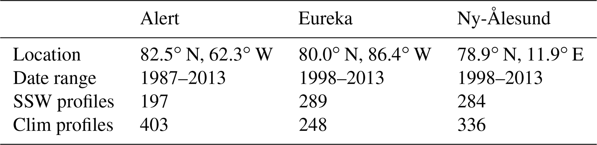
Table 1 The geographic latitude and longitude coordinates of the ozone sonde sites included in this study and the date range, together with the number of profiles used in calculating station mean ozone vertical profiles (100–1000 hPa) during all SSW events (0 to + 70 d around an SSW central warming date) and for a station climatology (clim) during the polar stratospheric dynamically active season. Note that the number of clim profiles included represents all soundings from December to April inclusive, excluding all SSW profiles and those in the preceding 20 d of an event onset. The locations and mean profiles are shown in Fig. 1. All ozone sonde profiles were convolved (averaged within ±20 hPa of the EMAC pressure levels) to reduce profile noise.

2.3 CAMS atmospheric composition reanalysis

The Copernicus Atmospheric Monitoring Service (CAMS) dataset is the latest atmospheric composition reanalysis product from the European Centre for Medium-Range Weather Forecasts (ECMWF), spanning the period 2003–2016 to date, which now supersedes the earlier Monitoring Atmospheric Composition and Climate (MACC) and CAMS-interim reanalyses (Inness et al., 2019a). A reanalysis product objectively combines observations and numerical modelling to comprehensively simulate weather- and climate-related variables based on a synthesized estimate of the state of the Earth's atmosphere. The development and insights gained from the earlier datasets enables the CAMS dataset to more accurately simulate the evolution of multiple chemical species within the atmosphere at enhanced horizontal (∼80 km) and temporal resolutions (3-hourly forecast fields and hourly surface forecast fields). Smaller biases and greater temporal consistency are found in the CAMS simulated fields of ozone (O₃) compared with that simulated by both MACC and CAMS-interim reanalyses, all of which are derived from satellite observations assimilated into the numerical model (Inness et al., 2019a).

2.4 Compositing procedures

For every time series, each nPJO and PJO SSW event (−30 to + 150 d of an event) is indexed for inclusion in the composites generated and, subsequently, for each 30 d period analysed. We use Table 1 from Karpechko et al. (2017) to index all PJO (n=11) and nPJO (n=11) events between 1980 and 2013 in our model simulations for inclusion in our composites. In calculating the climatological composites, the indexing for each event is applied to all years in calculating an average over the 34-year time series (1980–2013). In examining regional shifts in mid-latitude ozone distributions (Sect. 5) and Arctic radiative impacts (Sect. 6), however, the multi-year average is computed after all SSW cases (−30 to +150 d of an event) are removed from each time series. This procedure removes any influence of seasonality in our evaluations.

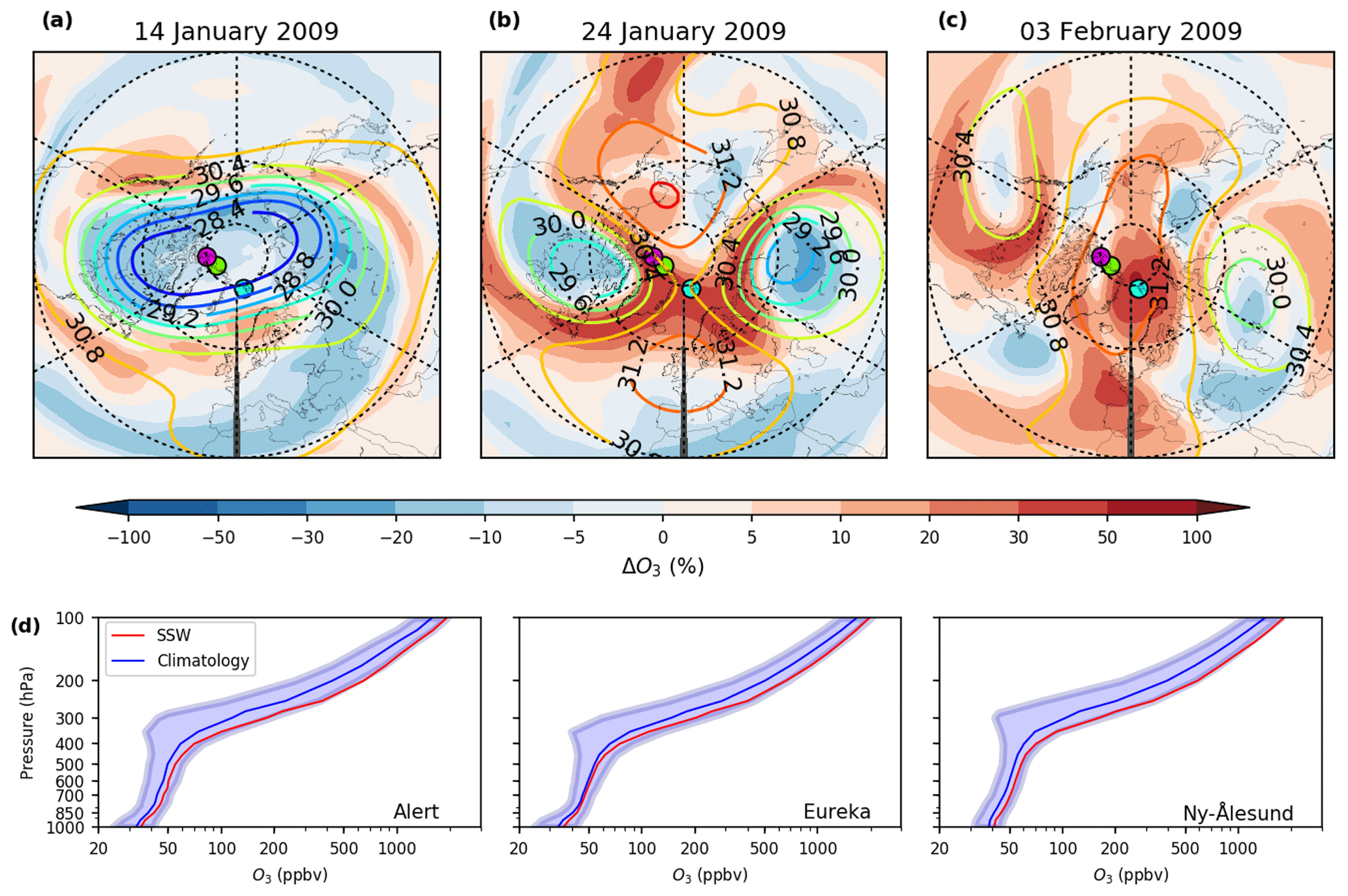
Figure 1 The 10 hPa geopotential height (km) (contours) and de-seasonalized ozone percentage anomalies (shading) over the Northern Hemisphere for (a) 10 d before; (b) the SSW central warming date; and (c) 10 d after a split-vortex, PJO-type SSW event (January 2009) from the CAMS atmospheric composition reanalysis. Ozone anomalies are calculated with respect to the 2005–2013 baseline period. Contour intervals are 0.4 km. (d) Ozone sonde (100–1000 hPa) climatology and SSW composite profiles for three long-running Arctic sites: Alert (green circle), Eureka (violet circle), and Ny-Ålesund (cyan circle), as marked on each map in panels (a)–(c). Mean SSW profiles were composited from all profiles within 0 to +70 d of an SSW central warming date, with all remaining profiles (excluding the 20 d prior to an event) used in compositing a mean climatology profile during the stratosphere's dynamically active season (December–April). The blue-shaded region represents 1σ around the climatological mean. The climatology is constructed excluding SSW events in each case.

2.5 Ozone distributions

Distributions of ozone for each region are calculated using a standard histogram-binning approach for the sub-class of SSW events (n=11) examined in Sect. 5. For each sub-column, the integrated amount of ozone (in Dobson Units, DU) at every 10-hourly model output time step within each 30 d period (n=72), multiplied by the number of model grid points in each selected domain, is used in generating a histogram of the data (which is divided into 20 bins). This yields a total number of data points of n=392 040 for North America, n=261 360 for Europe, and n=629 640 for Asia. The SSW and climatological distributions (excluding SSW events as defined within −30 to +150 d of an event) are then compared. In determining the statistical robustness of the results, a bootstrapping procedure involving resampling with replacement (Wilks, 2011) was implemented (i.e. the original pool of values is used for every resample) to yield 95 % confidence intervals around the median and the 90th percentile and 95th percentiles of each distribution (Tables S1–S4 in the Supplement for O₃S and S5–S8 in the Supplement for the ozone (O₃) tracer). Each event is considered to be an independent sample only (resulting in 11 SSW and 11 climatological cases) to remove any effects of spatial and temporal autocorrelation. Bootstrapping was performed over a standard number of iterations (10 000) to assign confidence intervals and to evaluate the extent to which the confidence intervals overlap. An additional common test of statistical significance (two-sample t test, with p<0.05) is performed separately in providing a thorough assessment.

2.6 Risk ratio (RR) calculation

The risk ratio (RR) of a 95th-percentile exceedance in the ozone distributions following a PJO-type SSW, with respect to climatology, is calculated for the three 30 d periods following the central warming (onset) date (lag 0: 0 to +30 d, lag 1: +30 to +60 d, and lag 2: +60 to +90 d) according to the approach by Zhang and Wang (2019, Fig. 1) in Sect. 5. From the derived cumulative ozone distributions, the 95th-percentile (0.95) level is identified for each climatological distribution at each lag. The corresponding value of ozone (X_ssw, in DU) is used to identify the change in the proportion of the SSW distribution above and below this 0.95 level. X_ssw is then used to determine the RR of an exceedance in ozone above this level, as calculated in Eq. (1):

$$\begin{array}{}\text{(1)}& \mathrm{RR}={\displaystyle \frac{\mathrm{1}-X_{\mathrm{ssw}}}{\mathrm{1}-\mathrm{0.95}}}.\end{array}$$

The RR may also be calculated by substituting in a threshold value (e.g. the 60 ppbv ozone standard) in place of the 95th percentile when surface ozone values are considered.

2.7 Radiative-impact calculations

A narrow-band radiative transfer code is used to calculate Fixed Dynamical Heating (FDH) stratospheric temperature changes due to ozone (O₃) and water vapour (H₂O) changes following the method of Fels et al. (1980), using an updated version of the code described by Forster and Shine (1997). In the shortwave, O₃ absorption is represented at 5 nm resolution in the ultra-violet and 10 nm in the visible. Near-infrared absorption by H₂O is included in 14 spectral bands (Chagas et al., 2001). The longwave code employs a 10 cm⁻¹ spectral resolution between 0 and 3000 cm⁻¹, with updates described in Shine and Myhre (2020); in addition to H₂O and O₃, present-day concentrations of carbon dioxide, nitrous oxide, and methane are included. Calculations assume clear-sky conditions and solar insolation for 70^∘ N on 27 January (lag +10 d calculation) and 8 March (lag +50 d calculation). Day-averaged insolation is calculated using a six-point Gaussian integration over the daylight hours. Both dates represent the mean lag date following the central warming (onset) date for all PJO-type SSW events (n=11) during the period of the EMAC simulation (1980–2013). The FDH calculations are run to equilibrium and so may be slightly larger in magnitude than transient FDH calculations (Forster et al., 1997). A composited polar cap (60–90^∘ N) mean temperature profile at a lag of 10 (averaged between 5–15) and 50 (averaged between 45–55) days after the central warming date of a PJO-type SSW, was extracted from EMAC as input to these calculations. For a later set of idealized FDH calculations (Sect. 6.2), in determining the seasonal dependence of radiative impacts due to lower stratospheric O₃ and/or H₂O anomalies, an artificially induced perturbation (centred around 100 hPa) was introduced, in which the five model levels above and below were adjusted according to a quadratic function.

3 SSW chemical perturbation signal

Before investigating potential air quality and radiative impacts associated with PJO-type SSWs using EMAC, the associated signal of enhanced polar stratospheric ozone is first confirmed from ozone sonde measurements. Over the last 9-year period of the EMAC simulation (2005–2013), overlapping with the CAMS reanalysis (excluding years 2003 and 2004 to remove any impact of model spin-up effects in our evaluations), the agreement between the model and reanalysis time series of Arctic (60–90^∘ N) ozone and water vapour is then quantified throughout the stratosphere–troposphere domain (1–1000 hPa). Such assessment is critical for deriving accurate interpretations of later results (Sect. 4 onwards).

3.1 Ozone

Figure 1a–c illustrate the poleward advection of anomalously high ozone, which occurs during a PJO-type SSW onset, for the January 2009 case, which constituted the most intense and prolonged event on record (Manney et al., 2009a), in accordance with the splitting of the SPV and displacement of residual vortices equatorward. As indicated on each spatial map, calculated mean ozone sonde profiles for the location of the three long-running, high-latitude ozone sonde monitoring stations detailed in Sect. 2.2 (representing climatological and SSW-impacted periods) are shown for the stratospheric dynamically active season (which we take as December–April, inclusive) in Fig. 1d. Although the composited SSW year profiles are well within the 1σ interval of non-SSW (climatological) years, a clear shift towards higher ozone is found throughout the profile, particularly for each site at heights above ∼350 hPa (mean tropopause height). Due to the sparse temporal sampling, such profiles have been composited over a full 5-month period in which SSW impacts can occur to yield a larger statistical sample. As such events likely only impact a shorter period of ∼ 2–3 months, it is therefore expected that such an approach may dilute the magnitude of the impact of the observed ozone enhancement in connection with such events. We note that the shift between the two profiles overall increases slightly when only including the PJO-type SSWs during this period, with the greatest difference interestingly being near the surface (Fig. S1). Whether this shift is physical (e.g. enhanced deep-STE events) or perhaps artificially inflated (e.g. due to temporal sampling bias) is an interesting question that merits further investigation on a case study basis, although the small sample size of events inhibits such an assessment in a composite-based approach.

The signal for such ozone enhancement (and overall agreement) according to both CAMS and EMAC can be visualized in Fig. 2, following both two nPJO and four PJO events for the 2005–2013 period, inclusive (a 9-year common baseline period for both datasets). The evolution in the de-seasonalized ozone anomalies (%) is shown as function of pressure (height), encompassing the upper stratosphere down to the surface (1–1000 hPa) for the polar-cap (60–90^∘ N) region. The 1–1000 hPa averaged Pearson correlation coefficient (r) over the whole period between each time series is 0.78, with values of between 0.86 and 0.94 between 10 and 300 hPa. Such values strongly support the notion that EMAC accurately simulates both interseasonal and interannual temporal variability in Arctic ozone abundance, particularly in the stratosphere; however, it is important to stress that CAMS does not constitute the truth (a detailed validation hindered by the sparse number of ozone sonde stations poleward of 60^∘ N). Overall, validation studies involving both ozone sondes and aircraft measurements (e.g. MOZAIC-IAGOS) do, however, demonstrate that free tropospheric ozone (∼ 350–750 hPa) is represented in CAMS to within an accuracy of ∼ ±10 % (mean bias) throughout the year over mid-latitudes and the Arctic (Christophe et al., 2019). The agreement is higher still in the stratosphere as satellite observations are directly assimilated in this region. Nonetheless, Fig. 1d provides evidence to confirm the signal of an ozone enhancement over a longer historical time span following such events.

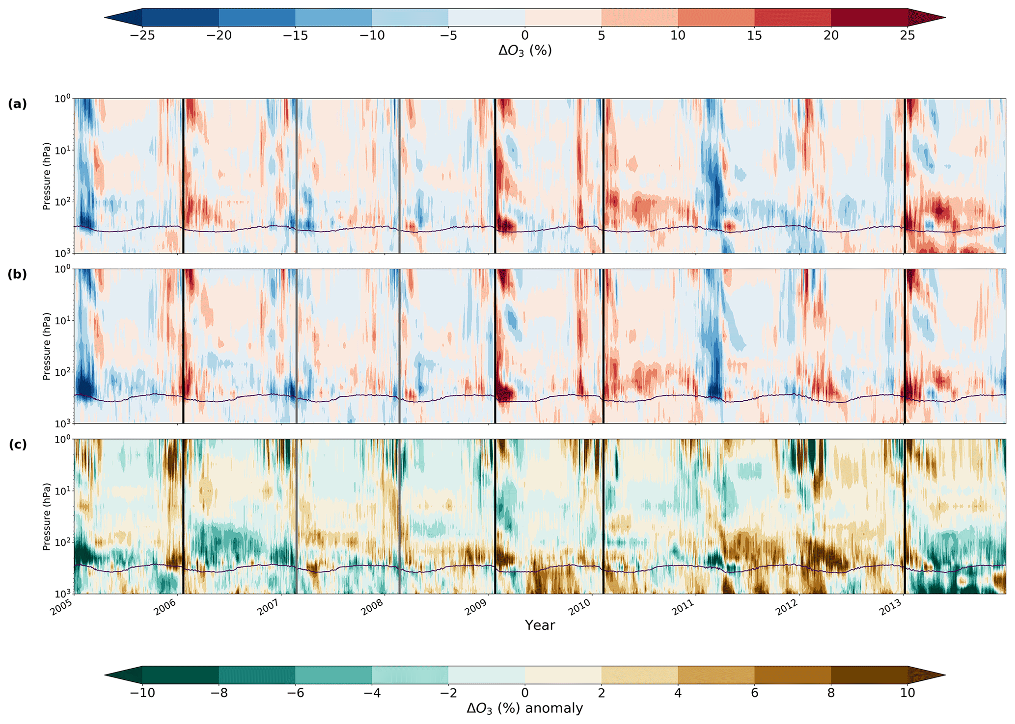
Figure 2 Vertical time evolution of polar-cap (60–90^∘ N) de-seasonalized ozone (%) anomalies for (a) CAMS reanalysis and (b) from the EMAC CCM specified-dynamics simulations relative to each respective climatology over the period 2005–2013. The difference between each anomaly time series (EMAC and CAMS) is, additionally, shown in panel (c). Vertical black (grey) lines denote the sub-class of PJO (nPJO) SSW central warming dates during the period. The 100 ppbv ozone contour (purple line) is included as a proxy for the tropopause pressure.

Importantly, the key features of the evolution of the CAMS ozone anomalies in the stratosphere following the major PJO sub-class of SSWs during the period, which notably includes the January 2009 and January 2013 vortex-split events, are well captured by EMAC. Moreover, EMAC-simulated variability in the evolution of stratosphere ozone anomalies during wintertime (the core of the stratospheric dynamically active season) in years without SSWs also closely resembles that of CAMS. Of note is the remarkable agreement and antisymmetric pattern with regard to the anomalies for both of the two major SSW events during this period, January 2009 and January 2013, with respect to the pronounced strong SPV during the 2010–2011 winter (Manney et al., 2011). Whilst the key features of the stratospheric ozone anomaly evolution following each sub-class of SSW are in agreement with other studies in the literature (e.g. de la Cámara et al., 2018b), this cannot be easily assessed here for the UTLS region due to differences in the vertical coordinate system adopted (pressure versus isentropic surfaces), the vertical domain, and the expression of anomalies (% versus ppbv). However, an earlier evaluation from Kiesewetter et al. (2010, Fig. 7), derived using a chemistry transport model driven by sequentially assimilated solar backscatter UV (SBUV) satellite ozone profile observations, provides quantitative agreement with the findings here for multiple SSW events between 1979 and 2007 (>25 % anomalies in lower-stratospheric polar ozone). Despite this, the lowermost isentropic surface assessed is 350 K (∼ 150–200 hPa) so the agreement down to tropopause height (∼ 320–330 K or 300–400 hPa) cannot be verified. The agreement between the CAMS reanalysis and the EMAC simulation gives confidence that the model performs well, particularly within the LMS (∼ 100–300 hPa), with a time series correlation (r value) between 0.85 and 0.90 over the 2005–2013 period.

This EMAC–CAMS difference panel (Fig. 2c) shows that the correspondence between each dataset is very reasonable (typically <5 % difference) around and just after the SSW dates during the 2005–2013 period (vertical solid lines). Following the January 2009 event, EMAC does suggest ozone values of up to 10 % greater than CAMS in the lower stratosphere, although the anomaly using CAMS is still >25 % relative to climatology in the LMS (∼ 100–300 hPa). The greatest disparity between the CAMS reanalysis and the EMAC simulation in the troposphere is evident during the summer of 2009 and from spring 2010 to the end of 2011, which did not coincide with any SSW occurrences. The evolution of the anomalies following the January 2013 SSW is, however, less consistently simulated between each dataset, although this is likely to be attributed to a change in the assimilated SBUV-2 data for ozone in the CAMS reanalysis from this year onwards (Christophe et al., 2019), resulting in a known discontinuity within the CAMS record. The disparity is largest in the troposphere, which, although it may seem counterintuitive, is highly likely to be related to propagation effects from the change in stratospheric assimilated information from the SBUV-2 platform since no direct information on the vertical distribution of ozone in the troposphere region is assimilated into the reanalysis (Inness et al., 2019a).

3.2 Water vapour

Figure 3 shows the temporal correspondence between EMAC and CAMS in the polar-cap-averaged (60–90^∘ N), vertically resolved (1–1000 hPa), de-seasonalized water vapour (H₂O) anomalies (%) spanning the 2005–2013 period. A very high overall agreement in each time series for the stratosphere and troposphere combined is indicated by a Pearson correlation coefficient (r) value of 0.81 (averaged between 1 and 1000 hPa), which is higher than for that computed for ozone. Such a value masks very large variations with pressure (height), with values of ∼0.7 at both 10 and 150 hPa, reducing to <0.5 in between at 50 hPa, and falling to as low ∼0.24 at 250 hPa. An r of ∼0.0 was computed close to the stratopause (∼1 hPa). This contrasts with consistently high values of >0.9 in the troposphere between 400 and 1000 hPa.

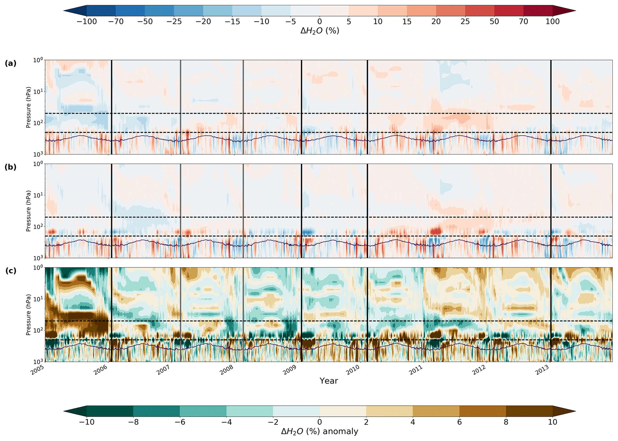
Figure 3 Same as Fig. 2 but for the vertical time evolution of polar-cap (60–90^∘ N) de-seasonalized water vapour (%) anomalies. We additionally mark the 50 and 200 hPa level (upper and lower dashed lines, respectively) to highlight common inflexion points between opposing sign anomalies following some of the SSW events during this period (most notably the PJO-type events).

The weaker correlation for the stratosphere can likely be related to the fact that H₂O is not assimilated in CAMS above the tropopause (∼ 100–300 hPa), beneath which specific humidity is assimilated from radiosondes, dropsondes, and aircraft observations (Hersbach et al., 2020); instead, a relatively simplistic parameterization of oxidation from methane, which is directly assimilated from satellite observations from multiple sources (SCIAMACHY, TANSO, and IASI) (Massart et al., 2014), is used for the representation of H₂O. Furthermore, it is quite widely established that reanalyses are notoriously poor at accurately simulating H₂O within the extratropical UTLS due to deficiencies in the simulation of cross-tropopause mixing and are often positively biased (too moist) (Davis et al., 2017). It is therefore reasonable to assume that EMAC has a better handle over the spatiotemporal variability of this species.

The 50 hPa level (indicated by the upper horizontal dashed line) appears throughout much of the time period to be close to an inflexion point in which the sign of H₂O anomalies are opposite above and below this region. Thus, a slight deviation in the height of this critical layer or subtle timing differences in the onset of anomaly changes between the CAMS reanalysis and the EMAC simulation may account for the reduced correspondence at this level. This is even more true for the 200 hPa level (lower horizontal dashed line), which is frequently close to the boundary between anomalously moist and dry conditions, particularly during winter. A dipole in this region is a common feature throughout the 9-year (2005–2013) period, with anomalies sometimes exceeding ±25 %. Following the major PJO-type SSWs over this period, which include January 2006, January 2009, and January 2013, an anomalously dry region is found for heights above 200 hPa, which overrides an anomalously moist region immediately below this level. It should be noted that this signal is not so pronounced following the other major PJO-type events (February 2010) during this period according to either EMAC or the CAMS reanalysis. This pattern is not consistent with the nPJO sub-class of SSW events during this period (February 2007 and February 2008) or with other winters during this period, such as in the 2010–2011 winter, which was characterized by an anomalously strong SPV. In the latter case, a particularly strong H₂O dipole anomaly is present, with the sign of the anomalies inverted with respect to three of the PJO-type SSWs (January 2006, January 2009, and January 2013). The fundamental reasons for the occurrence of a dipole in this region, which is most prevalent during winter, are unclear but most likely relate to a vertical displacement in the mean tropopause height over the Arctic region and/or changes in poleward advection of moisture-rich air masses from lower latitudes.

4 Chemical perturbations in the tropopause region

Having verified that the EMAC-simulated evolutions in Arctic ozone and water vapour closely resemble the ozone sonde and CAMS reanalysis (Figs. 2 and 3), with the caveat that agreement between the model and CAMS is lower below the tropopause, we use EMAC to examine composition changes during SSWs for the 1980–2013 period to obtain more robust statistics through the inclusion of more events.

4.1 SSW chemical composition evolution

Figure 4a–c show the composite evolution of de-seasonalized anomalies (%) of ozone (O₃), water vapour (H₂O), and the vertical residual velocity (${\stackrel{\mathrm{‾}}{w}}^{*}$), a metric for changes in the strength of polar downwelling (where downwelling is indicated by negative ${\stackrel{\mathrm{‾}}{w}}^{*}$) from the upper stratosphere to the surface (1–1000 hPa) over the period 1980–2013, split into nPJO (n=11) and PJO (n=11) events¹. The temperature composites for both nPJO and PJO events are shown in Fig. S2. The relative anomalies in both O₃ and H₂O are more pronounced and protracted during PJO-type events, consistent with the resultant larger perturbation to the dynamical state of the lower and middle stratosphere (Hitchcock et al., 2013). The onset (taken as the central warming date denoted by the solid black lines in Fig. 4) of a PJO-type SSW is characterized by the emergence of positive O₃ anomalies (∼ 5 %–20 %) in the middle and lower stratosphere (10–100 hPa) and in the upper stratosphere (1–3 hPa) just a few days later (ΔO₃ >25 %), which is well established from previous stratospheric ozone SSW composite analyses (de la Cámara et al., 2018b; Haase and Matthes, 2019). A larger, more prolonged relative enhancement (ΔO₃ >25 % persisting for ∼50 d) is seen in the LMS (tropopause to 100 hPa), which has so far received little attention. Concurrently, significant anomalies in H₂O are found around the time of the SSW onset, largely confined to the LMS region and lasting for around 50–70 d. A clear drying signal (∼25 %) is evident around 120–200 hPa, with a moistening signal of approximately equal magnitude immediately below, just above the tropopause (∼ 200–350 hPa). Only a modest enhancement of up to ∼10 % in O₃ and $\sim \pm$ 10 % in H₂O is evident following nPJO events.

Figure 4 Vertical time composites of polar-cap (60–90^∘ N) averaged (a) ozone (O₃), (b) water vapour (H₂O), and (c) residual vertical velocity (${\stackrel{\mathrm{‾}}{w}}^{*}$) de-seasonalized anomalies (%) for nPJO-type and PJO-type SSWs (each of which with n=11 events) from EMAC for the time period 1980–2013. The anomalies are expressed as percentages, with the exception of the residual vertical velocity (${\stackrel{\mathrm{‾}}{w}}^{*}$) anomalies, which are given in units of metres per second (m s⁻¹) (zero contour represented by solid purple line). Statistical significance at the 95 % level is indicated by stippling. The World Meteorological Organization (WMO)-defined thermal tropopause is displayed for reference in each panel (solid blue line).

The long persistence timescales of the composition anomalies in the LMS reflect the dominant role of radiative processes as the reversal of the stratospheric winds suppresses the propagation of planetary waves into the stratosphere (Hitchcock et al., 2013). The evolution of polar-downwelling (${\stackrel{\mathrm{‾}}{w}}^{*}$) anomalies shows a period of accelerated descent throughout the Arctic stratosphere immediately prior to an SSW in all cases. This is rapidly followed by a period of anomalously weak polar downwelling in the upper stratosphere that gradually propagates down as the SSW evolves (in the case of PJO events). This anomalous evolution in polar downwelling helps explain the establishment of the anomalies in O₃ and H₂O in the LMS and perhaps also influences their persistence, but this aspect would need to be studied further. The persistence of such simulated changes in composition are consistent with the delayed recovery of the SPV for PJO events, which are known to have larger impacts on the tropospheric circulation (Hitchcock et al., 2013; de la Cámara et al., 2018a). Although an increase in tropospheric ozone is shown during these events, the lack of statistical significance leads us to further attempt to isolate the stratospheric influence.

4.2 Impact on stratosphere-to-troposphere exchange (STE) of ozone

To elucidate whether STE of ozone is enhanced as a result of the anomalous enrichment in LMS ozone, we use an additional model tracer which only tracks ozone of stratospheric origin (O₃S). We also derive and explore changes in the evolution of the tropospheric fraction of ozone of stratospheric origin (O₃F) using this tracer (O₃F = O₃S $/$ O₃ ×100). The de-seasonalized anomalies (%) evolution for O₃S and O₃F are shown for both the nPJO-type and PJO-type event distinction (Fig. 5). A signal for enhanced STE is apparent for ∼ 0–80 d following an SSW, although the entrainment of enhanced O₃S into the troposphere is initially confined to the upper troposphere (300–500 hPa). Deeper penetration of O₃S into the troposphere, more clearly shown in the anomalies of O₃F, is evident from around 20 d after the SSW central warming date, extending out to ∼80 d. Given a photochemical lifetime of ozone in the free troposphere around 3 weeks (Lelieveld et al., 2009) and a statistically significant negative Arctic Oscillation pattern at least following PJO-type events (Hitchcock et al., 2013), favouring net equatorward transport in the troposphere, such a prolonged signal for elevated O₃S in the lower troposphere can only be attributable to enhanced STE for a sustained period (note that this tracer is subject to the same chemical sink reactions as the full ozone field).

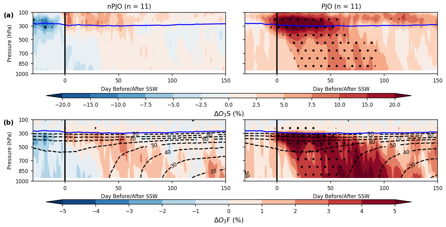
Figure 5 As Fig. 4 but for (a) ozone of stratospheric origin (O₃S) and (b) the fraction of ozone of stratospheric origin (O₃F = O₃S $/$ O₃ ×100) de-seasonalized anomaly (%) evolutions for nPJO-type SSWs (n=11) and PJO-type SSWs (1980–2013) from EMAC for the time period 1980–2013. The EMAC climatological O₃F (1980–2013) is overlaid (dashed contours) for reference in panel (b). Note that this seasonally evolving field is offset between nPJO and PJO cases since the mean SSW onset date differs between each event category (nPJO: 11 February and PJO: 17 January).

For both composites, a peak response around 50 days after the SSW onset date is apparent, with indication of an enhancement in O₃S throughout the troposphere and elevated near-surface O₃S which may impact air quality (see Sect. 5). The maximum increase in O₃S is on the order of ∼ 5 %–10 % for PJO-type events, particularly near the surface, which equates to a change in the fraction of stratospheric ozone (O₃F) of >5 %. For this subset of events, the mean SSW onset date (17 January) is sufficiently early that this enhancement typically occurs when >50 % of tropospheric ozone is sourced from the stratosphere, at least initially. In contrast, a minimal enhancement of O₃F (∼ 1 %–2 %) for a much shorter duration is shown to follow nPJO events, which is even less significant as the fraction of ozone originating from the stratosphere is climatologically smaller (∼ 30 %–50 %) just a few weeks later (mean nPJO event onset date: 11 February) as winter transitions to spring. These findings support the notion that SSWs exert a downward influence not only dynamically on tropospheric circulation (Baldwin and Dunkerton, 1999; Scaife et al., 2016) but also chemically on tropospheric composition, though this is primarily for the PJO-type events. The delay of this influence by 50–80 d after the SSW onset ensures a maximum impact extending into the photochemically active season (spring) (Logan, 1985; Lelieveld and Dentener, 2000). As shown in Williams et al. (2019), the seasonal peak in lower-tropospheric O₃F over the Arctic occurs in winter despite a maximum in tropospheric ozone during spring (>50 ppbv) since the partition of ozone from the stratosphere (O₃S) is similar in both seasons (∼ 20–30 ppbv), meaning O₃F is typically ∼10 % less in spring (∼ 40 %–50 %).

5 Mid-latitude tropospheric ozone enhancement

The level of tropospheric entrainment of anomalously high ozone values in the LMS following PJO-type events over the Arctic (60–90^∘ N) region is next assessed using EMAC over the populated mid-latitude regions of the Northern Hemisphere, the hemisphere in which STE is most pronounced (Holton et al., 1995). This investigation is particularly pertinent to understanding how such events may affect the propensity for infringements of surface air quality standards. Although EMAC has a coarse horizontal resolution (∼2.8^∘), therefore precluding a detailed assessment, it is possible to gauge the likelihood and approximate magnitude of an increase in background tropospheric ozone, together with the associated risk enhancement of surface ozone exceedances above regulatory standards. The use of a fully interactive specified-dynamics ozone simulation, together with an accompanying stratospheric-tagged ozone (O₃S) tracer, makes it possible to isolate a downward-propagating signal in ozone separate from modulating tropospheric influences (of both dynamical and chemical origin). In this section, shifts in composited regional ozone distributions for both non-SSW (climatological) versus SSW-impacted years are examined at multiple lags following the event onset (central warming date) from the UTLS down to the surface for the PJO sub-class of events earlier identified. This analysis is then repeated in an idealized case to help further extract and quantify the signal in the ozone tracer separately from potential confounding effects arising from the response of tropospheric dynamical and chemical processes, as well as the presence of any underlying temporal trends (e.g. driven by trends in ozone precursor emissions) in the dataset with respect to the signal strength.

5.1 Regional ozone distribution shifts

To ascertain changes in LMS and tropospheric ozone following PJO-type SSWs over different mid-latitude (30–70^∘ N) regions of the Northern Hemisphere (Europe, North America, and Asia), where enhanced stratospheric influx has the potential to affect air quality, distributions of the integrated quantity of ozone (Dobson Units, DU) are calculated for different select sub-columns. We include the SSW (solid lines) and climatology (dashed lines) composite distributions, using the O₃S tracer, for the LMS (100–300 hPa), upper troposphere (300–500 hPa), an approximation for the planetary boundary layer (PBL) (900–1000 hPa), and the model surface level, averaged over the 0–30, 30–60, and 60–90 d periods following the SSW central warming date (Fig. 6) (see Sect. 2.4 (Data and methods) for details on composite construction). For completeness and to conduct a surface air quality impact evaluation, we replicate the analysis for the full ozone field (Fig. S3). We employ a bootstrapping (resampling with replacement) procedure (Wilks, 2011) to evaluate the statistical robustness of the differences between the SSW and corresponding climatological distributions, as well as conducting a paired two-sample t test (results are shown in Tables S1–S4, and further details of the approach are included in Sect. 2.5). This analysis is repeated for the full ozone field (Tables S5–S8). We additionally calculate risk ratios (RRs) (displayed values) with regard to the likelihood of an exceedance of the 95th percentile for each SSW distribution (using Eq. 1) with respect to each corresponding climatological distribution at each lag. An exception is that used for the model surface level in the O₃ case (Fig. S3), where we also substitute in the 60 ppbv threshold in place of the 95th percentile for each region (as mentioned in Sect. 2.6).

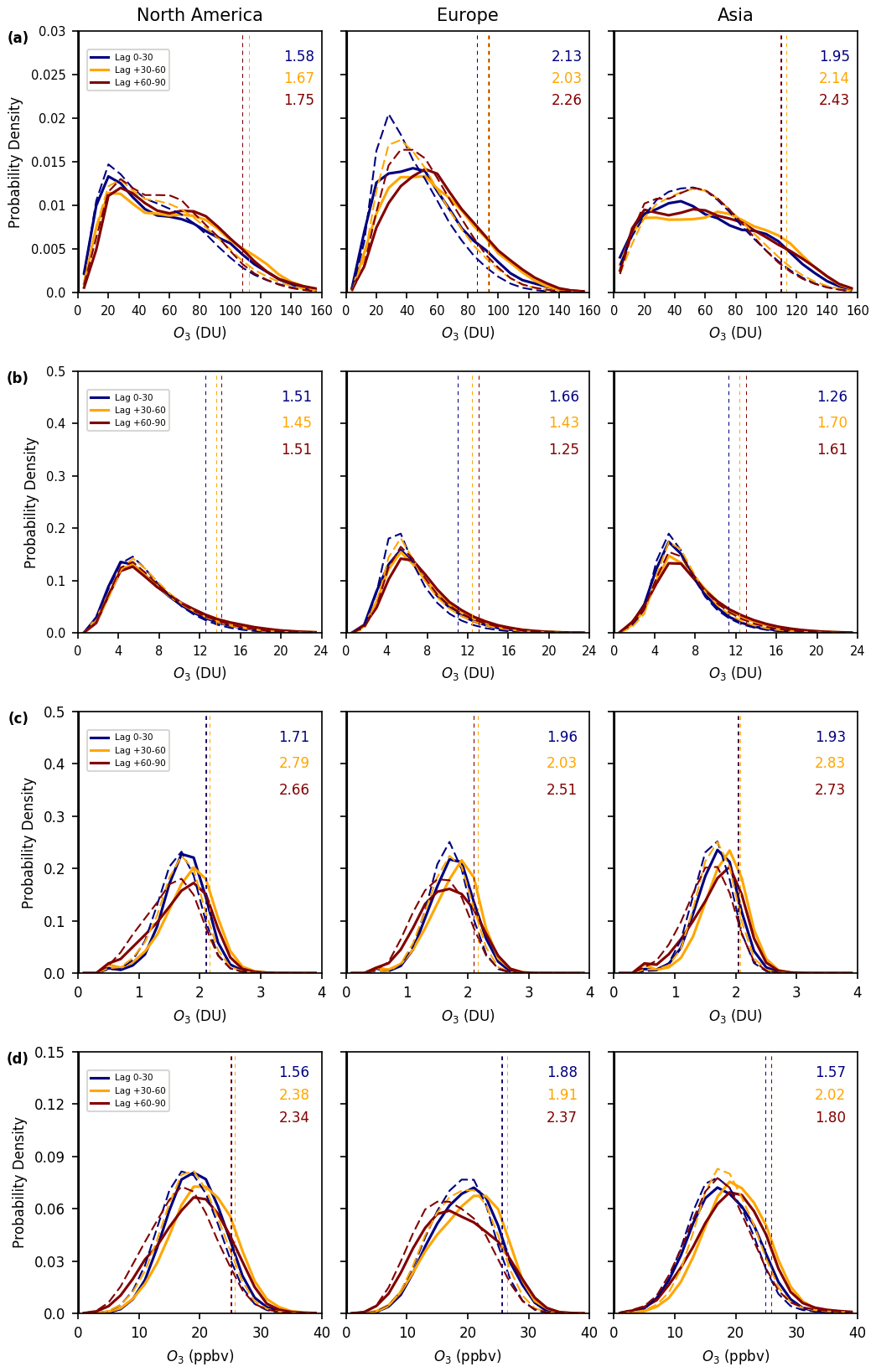
Figure 6 Time–area averaged distributions for North America (30–70^∘ N, 150–60^∘ W), Europe (30–70^∘ N, 30^∘ W–30^∘ E), and Asia (30–70^∘ N, 30–180^∘ E) for (a) the LMS (100–300 hPa), (b) upper troposphere (300–500 hPa), (c) the planetary boundary layer (PBL) (900–1000 hPa) sub-column ozone of stratospheric origin (O₃S), and (d) simulated surface O₃S mixing ratios (ppbv) for lags of 0–30 d (blue lines), 30–60 d (orange lines), and 60–90 d (red lines) following the SSW central warming date. Solid lines represent SSW composite distributions, and dashed lines represent the composite generated from the EMAC climatology (1980–2013), excluding SSW events. Risk ratio (RR) values of the probability of an exceedance in the 95th-percentile level of each climatological distribution (dashed vertical lines) are indicated.

A noticeable shift of the O₃S SSW distributions is apparent for the LMS over each region with respect to climatology (Fig. 6a), with a statistically significant (p<0.05) shift towards higher values in all cases pertaining to the median and the 90th and 95th percentiles of each distribution (Table S1). Given the proximity to the stratosphere in this region, Fig. S3 reflects this shift to a nearly equal magnitude for the full ozone distributions, and the statistical significance (p<0.05) is again evident from Table S5. Ultimately, this confirms that the overall enhancement in ozone evident from the polar-cap composites (Fig. 4) indeed extends over mid-latitude regions following this sub-class of events. A more stringent measure of statistical significance is to discern this only where the calculated 95 % confidence intervals, as calculated through the bootstrapping approach, do not overlap (e.g. Schenker and Gentelman, 2001; Payton et al., 2003) for each statistic in every case (Tables S1 and S5). Using this measure, the shift in the median and the 90th and 95th percentiles is again significant in every case for Europe and in most cases for both Asia and North America (the exceptions are mostly between 0 and 30 d when the impact of the SSW likely has yet to peak). As an additional metric to quantify change in the proportion of the distributions in exceedance of the 95th percentile according to climatology, RR values of between ∼2.0 and 2.5 for Europe and Asia equate to a doubling or more in the frequency of grid point incidences above this threshold for both O₃S (Fig. 6a) and the full ozone tracer (Fig. S3a). Values between 1.5 and 1.75 for North America translate to a lesser 50 %–75 % increase, which still also constitutes a substantial shift.

The shift of ozone distributions in the upper troposphere (300–500 hPa) for both O₃S (Fig. 6b) and O₃ (Fig. S3b) are qualitatively consistent in relation to those in the LMS (100–300 hPa), further confirming that more ozone from the stratosphere is entrained into the free troposphere following such events according to EMAC. Whilst the result is statistically significant for O₃S for the 60–90 d lag (Table S2), associated with a corresponding sub-column increase of ∼ 1–2 DU, the significance of the signal for O₃ is marginal. This is highlighted by the presence of overlap between the 95 % confidence intervals for each respective climatological and SSW distribution for each statistic bootstrapped over despite largely contradictory suggestions from the two-sample t test performed (p values generally less than 0.05). A notable exception to this is for the 95th-percentile statistic over North America during this period (Table S6). For both O₃S and O₃, however, the frequency of a 95th-percentile exceedance in the SSW distributions nevertheless ranges between a 25 % and 70 % increase relative to climatology according to the calculated RR values in Fig. 6 for O₃S and Fig. S3 for O₃, respectively (values are very similar in both cases).

The enhancement signal remains discernible for the approximation of the PBL used (here defined as 900–1000 hPa; Fig. 6c), which is consistent with model estimates of the depth of this layer during winter and springtime (McGrath-Sprangler et al., 2015) and the model surface level (Fig. 6d) in the case of O₃S, but it is largely indistinguishable for O₃ (Fig. S3c, d). Interestingly, a paired two-sided t test applied to the distributions implies that such a signal is statistically significant in all cases for O₃S (Tables S3 and S4); this also holds true in most cases where this is inferred according to when the 95 % confidence intervals do not overlap, except during the first 30 d lag period when the impact of such events would not be expected to yet manifest. It is particularly interesting to note that a statistically significant signal according to both measures, computed for all three statistics, is detectable following such a sub-class of events according to the EMAC model for both the 30–60 and 60–90 d lag periods, whereas this was most apparent for the upper troposphere for the 60–90 d lag interval. This finding could reflect an earlier enhancement near the surface, courtesy of deep STT transport events, in which the stratospheric influence is at a maximum in late winter–early spring, as reported by many studies (e.g. Stohl et al., 2000; Lefohn et al., 2012; Lin et al., 2012; Škerlak et al., 2014), versus a slower background ozone enhancement driven by the large-scale descent that would be detectable only later (Lefohn et al., 2011). In contrast to the O₃S finding, statistical significance cannot be inferred using either measure in almost all cases for the O₃ tracer (Tables S7 and S8). As shown in Sect. 5.2, however, it is reasonable to conclude that other factors may dampen the overall background signal for a near-surface ozone enhancement following such events (which are still only, in part, isolated when examining the O₃S tracer).

Focusing on the change in the median and the 90th and 95th percentile values for the model surface level (volume mixing ratio units of ppbv), an increase of ∼1.5 to 3 ppbv of O₃S amount would translate to a maximum ozone concentration increase of ∼ 3–6 µg m⁻³. This equates to ∼ 5 %–10 % of the 2021 World Health Organisation (WHO) surface air quality standards, which are set at 60 µg m⁻³ or 30 ppbv for a mean 8 h interval during the season of peak surface ozone concentration (WHO, 2021). RR values of a 95th percentile exceedance according to constructed climatology are calculated for both the PBL (900–1000 hPa) and model surface level to be, furthermore, very close to 1 in the case of the O₃ tracer but on the order of ∼1.5 to 3 (50 %–150 % increase) for the O₃S tracer. This finding is certainly of note and likely of greater concern for the impact on surface air quality resulting from more localized, episodic events, although this requires further investigation using much-higher-resolution tools and datasets. We next attempt to further isolate the signal of a background enhancement in near-surface ozone by artificially separating out potential confounding influences that may dampen the signal when using the ozone tracer of EMAC.

5.2 Signal in background near-surface ozone

Despite our efforts to circumvent the issue of limited sample size (i.e. 11 PJO-type SSW events during the 1980–2013 period) using a statistical bootstrapping approach, the lack of a statistically significant impact on regional distributions of Northern Hemisphere mid-latitude lower-tropospheric ozone is not an unexpected result when using the full ozone (O₃) tracer. Whilst the use of the stratosphere-tagged ozone (O₃S) tracer helped confirm and isolate the signal of enhanced stratospheric influence, which is clearly robust according to both a paired two-sided t test and the bootstrapping approach employed here, it is more meaningful to be able to verify and quantify the signal for O₃. Aside from the caveat of using a coarse-resolution (∼ 2.8^∘) simulation, it is possible to artificially separate the influence of potential confounding factors, which give rise to the inherently large variability in tropospheric ozone, in addition to possible underlying trends within the dataset to further extract the signal. We explore this by first subtracting the O₃S partition from the full ozone amount for the SSW composites, leaving the residual amount of tropospheric-origin ozone, and then adding the O₃S partition from the constructed climatological composites (non-SSW years) in creating a set of pseudo-climatological ozone distributions. Figure 7 shows the results of comparing these artificially constructed ozone distributions relative to composited SSW distributions for each region (North America, Europe, and Asia) and for each lag: 0–30, 30–60, and 60–90 d for the PBL (900–1000 hPa sub-column) and model surface level.

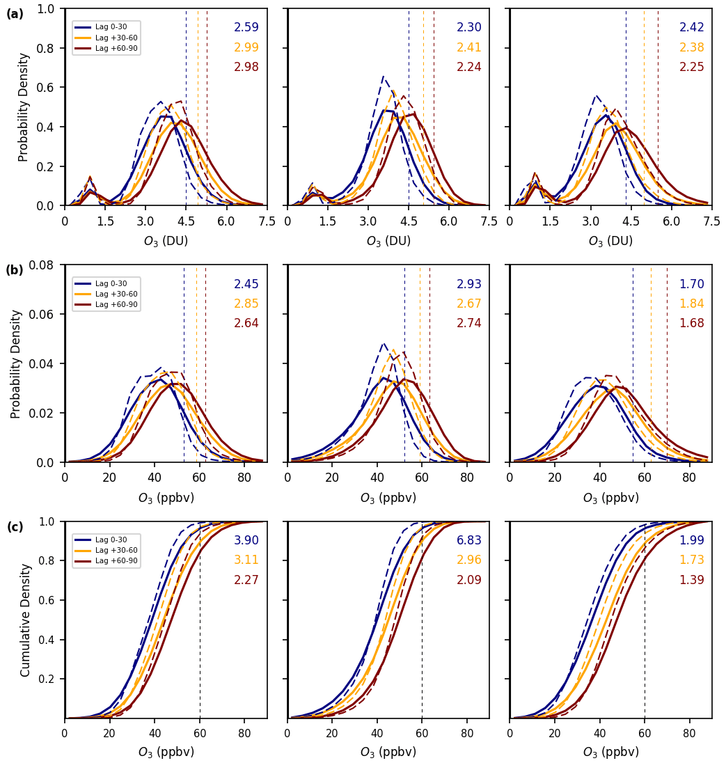
Figure 7 Time–area averaged distributions for North America (30–70^∘ N, 150–60^∘ W), Europe (30–70^∘ N, 30^∘ W–30^∘ E), and Asia (30–70^∘ N, 30–180^∘ E) for (a) the planetary boundary layer (PBL) (900–1000 hPa) sub-column (DU) and (b) the simulated surface O₃ mixing ratio (ppbv) for lags 0–30 d (blue lines), 30–60 d (orange lines), and 60–90 d (red lines) following the SSW central warming date. The cumulative ozone distributions for the model surface level are additionally shown (c) to more clearly highlight an overall shift towards anomalously high ozone values. Solid lines represent again the SSW composited distributions, and dashed lines represent the corresponding pseudo-climatological distributions generated from the EMAC climatology for the ozone of stratospheric origin (O₃S) component (1980–2013), excluding SSW events. Risk ratio (RR) values of the probability of an exceedance in the 95th-percentile level of each climatological distribution (dashed vertical lines) are indicated, with the exception of panel (c), where the values represent an RR increase in the likelihood of an exceedance in the 60 ppbv threshold (a typical surface air quality standard).

The result is that, when using this method to create pseudo-climatological composites which are temporally consistent with the event occurrence dates (i.e. both SSW and climatological constructed composites contain the same amount of ozone derived from tropospheric production sources), the shift in each ozone distribution is more pronounced. This highlights that the enhanced stratospheric influence signal, as confirmed using the O₃S tracer (Fig. 6) and tested for statistical robustness (Tables S1–S4), is present within the EMAC full ozone field. As quantified using the risk ratio metric (Eq. 1) to assess the probability change in the exceedance of the 95th-percentile (Fig. 7a–b) or the 60 ppbv threshold for the model surface level (Fig. 7c), the values are significantly larger than for the compositing method used in Sect. 5.1 when using the O₃ tracer (Fig. S3c–e) and are generally higher even with respect to the equivalent evaluation using O₃S (Fig. 6c–d).

In terms of the upper tail end of each pair of distributions, the impact is most pronounced for the earliest lag (0–30 d), which might be expected as enhanced STT transport events are likely to occur sooner than any overall background enhancement into the free troposphere, facilitated by slow overall descent, as mentioned previously. The latter would have a larger impact on the overall distribution as opposed to the upper tail end. Whilst there are some significant differences in the risk ratio changes for each given lag between Europe and North America, typically a factor of 2 to 3 increase (or equivalent to a 100 % to 200 % increase) in the number of incidences above either the 95th percentile of the pseudo-climatological distributions (or 60 ppbv threshold additional for the model surface level), it is notable that the signal is much weaker for Asia (risk ratios between 1.5 % and 2.0 % or 150 % and 200 % increase for the surface level). Such regional disparity is not evident from either Figs. 6 or S3 and could therefore be explained as a result of fixing the proportion of ozone formed in the troposphere for each pair of distributions. However, the relative role of tropospheric processes (dynamical or chemical) that may attenuate the signal with respect to possible underlying trends in the data cannot be assessed here, although more detailed investigation is warranted in this regard.

6 Radiative impacts of Arctic ozone and water vapour perturbations

The ozone (O₃) and water vapour (H₂O) anomalies associated with SSWs will furthermore have radiative impacts which are likely not well represented in present-day numerical weather prediction (NWP) models, potentially limiting the forecast skill of the overall simulation and tropospheric response to such events. In the case of ozone, many NWP models generally adopt a zonal-mean, monthly mean climatological representation within their radiation schemes owing to both computational constraints and untested accuracy of any 3D prognostic scheme performance (e.g. Monge-Sanz et al., 2022), although leading centres such as ECMWF are in the process of implementing this operationally in both NWP (10–15 d) and sub-seasonal forecasts (Williams et al., 2021). Whilst water vapour is much better represented in NWP models, particularly beneath the tropopause, sharp discontinuities in the UTLS region are particularly troublesome to resolve, and this is highly significant as this region is radiatively very sensitive (e.g. Riese et al., 2012; Shepherd et al., 2018). To explore and quantify such radiative effects of composited perturbations in mean profile Arctic ozone and water vapour perturbations following PJO-type SSWs, calculations are performed for ∼10 and 50 d after such events occur using the FDH technique (see Sect. 2.7). The radiative sensitivity of idealized UTLS ozone and water vapour perturbations over the Arctic is also investigated through evaluating the results of a series of evaluations at key intervals during the stratospheric dynamically active season (December–April).

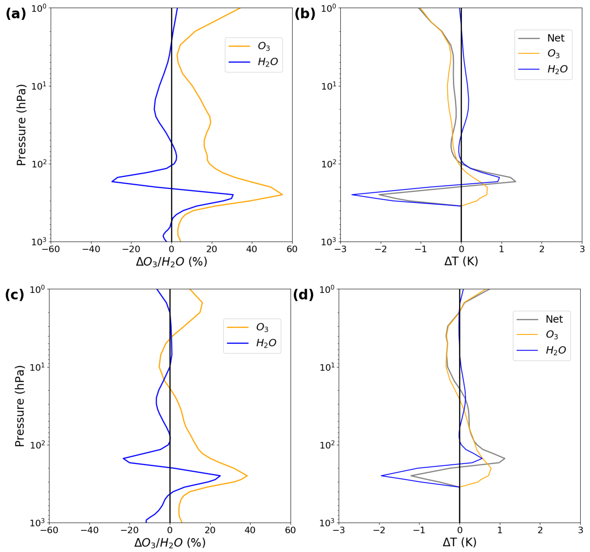
Figure 8 Polar-cap averaged (60–90^∘ N) (a) mean perturbation to the vertical profile in terms of ozone and water vapour (%) and (b) the resultant radiatively driven stratospheric temperature change averaged 5 to 15 d after a PJO-type SSW (composite of 11 events over the period 1980–2013). The equivalent is shown below panels (c) and (d) when averaged 45 to 55 d after the mean event onset date. The solid grey line represents the net temperature change due to these composition anomalies. The FDH temperature changes are only computed at heights above the tropopause (set as 300 hPa for these calculations).

6.1 SSW radiative impacts

We calculate the radiatively driven component of stratospheric temperature changes by performing FDH calculations for the subset of PJO-type SSW events (n=11) during the period 1980–2013 using the EMAC model results. Figure 8 shows the polar-cap (60–90^∘ N) mean O₃ and H₂O anomaly profiles (1–1000 hPa) averaged 5–15 and 45–55 d after the central warming (onset) date, together with the calculated FDH temperature changes (ΔT), due to each species separately and the total change. Note that the calculations are performed for profile averaged O₃ and H₂O over a 10 d interval to remove any impact of daily fluctuations which can be large, particularly during the early stages of such an event. The most significant temperature changes after the SSW onset (Fig. 8a–b) are found to occur in the LMS (tropopause to 100 hPa), in accordance with the largest changes in O₃ and H₂O with respect to climatology, as well as the high radiative sensitivity to composition changes in this atmospheric region. A warming signal of ∼1.5 K is evident around 150–200 hPa, mostly due to the reduction in H₂O, with a cooling signal of ∼2 K centred around 250–300 hPa, induced by the perturbation to H₂O but moderated slightly by the radiative-warming effect of O₃ in this region. An enhancement of O₃ in the middle to lower stratosphere (10–100 hPa) results in a slight cooling (up to ∼0.4 K), which is slightly offset by the radiative effect of H₂O (up to $\sim +\mathrm{0.1}$ K), leading to a net cooling of ∼ 0.2–0.3 K. This slight cooling, despite the increase in ozone at these levels, is mostly due to the change in upwelling longwave radiation due to the larger (in percentage terms) increase in ozone in the lower stratosphere. This deprives the mid-stratosphere of upwelling infrared radiation which would otherwise warm this region; the reverse effect (where a lower-stratospheric ozone depletion leads to cooling of the lower stratosphere but a warming of the mid-stratosphere) has been noted by Ramaswamy and Bowen (1994) and Shine (1996), for instance. Given that this corresponds to late January, changes in the longwave radiation budget will dominate over changes in the shortwave radiation budget. Above 10 hPa, O₃ changes alone lead to a cooling tendency that increases with altitude (∼>1 K at 1 hPa). The additional set of calculations averaged 45–55 d after the central warming (onset) date (Fig. 8c, d) yields similar results, indicating that such radiative effects, if ignored, would lead to a systematic temperature bias in NWP models, with possible knock-on consequences for wind fields. The ozone anomaly profile more closely matches the heating profile due to ozone throughout the stratosphere as solar insolation is much greater by early March. We note that the heating effect due to ozone between 200 and 300 hPa is slightly larger for this later lag despite a reduction in the percentage anomaly (from nearly 60 % to just under 40 %).

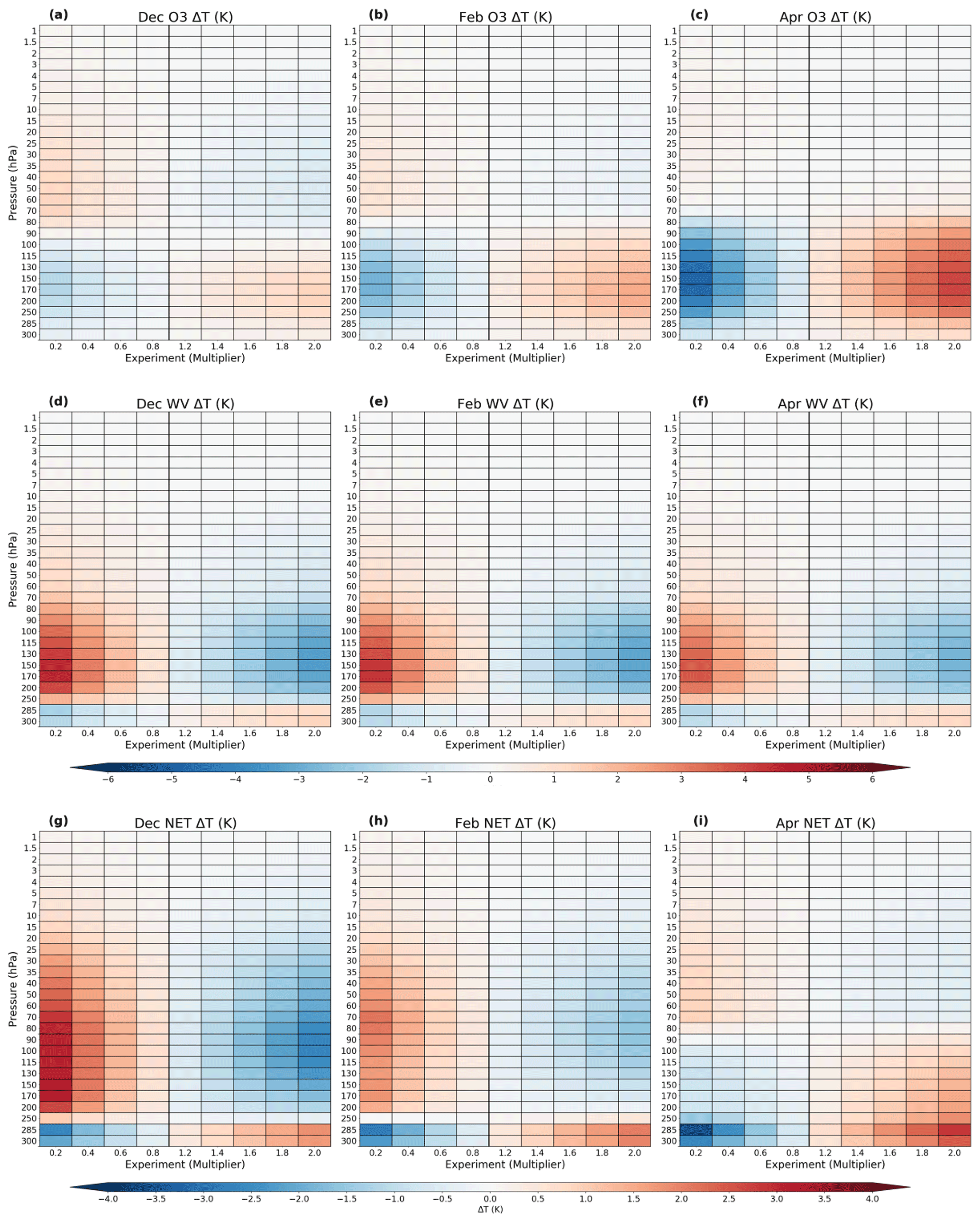
Figure 9 The idealized change in stratospheric temperature due to deviations in lower-stratospheric (∼ 70–150 hPa) ozone and/or water vapour with respect to (a, d, g) mid-December, (b, e, h) mid-February, and (c, f, i) mid-April climatology is shown as a function of pressure (y axis) and perturbation increment (multiplier) (x axis). The solid black line represents a zero change in UTLS ozone abundance from climatology, with results shown for up to an 80 % reduction (multiplier of 0.2) and up to a 100 % increase (multiplier of 2.0) from left to right in each panel.

6.2 Idealised radiative impacts

The sensitivity of the lower-stratospheric composition-induced modulation to the vertical profile in Arctic stratospheric temperature is next elucidated as a function of both altitude and perturbation increment during the evolution of the stratospheric dynamically active season (December–April). FDH-calculated changes in the mean polar-cap (60–90^∘ N) vertical temperature profile, resulting from an idealized perturbation in lower-stratospheric (70–150 hPa) ozone and/or water vapour (see Sect. 2.7 for details), are shown in Fig. 9 with respect to the mid-December, mid-February, and mid-April EMAC climatology (1980–2013). The increased radiative importance of ozone later in the season as solar input is greatly enhanced (increased shortwave heating) and the slight reduction in the water vapour radiative effect are clearly evident. The opposing sign of the radiative effect from each constituent acts to offset the net temperature response to a varying degree within the UTLS. Early in the season (December), however, water vapour exerts a dominant radiative control. This manifests in Fig. 9g as a warming of up to 3.5 K and a cooling of −3 K between ∼70 and 150 hPa for an 80 % reduction and 100 % enhancement in both ozone and water vapour, respectively. The magnitude of this tendency gradually decreases with height above the 70 hPa level (upper bound of the perturbed region) as this region is only influenced by the non-local radiative effects. The tropopause region (∼250 hPa), on the other hand, is instead marked by an opposing radiative response (dipole) beneath this critical level (i.e. a cooling and warming of up to ±3 K for an −80 % and a 100 % perturbation increment, respectively). These tendencies are similar to Fig. 9h for mid-February, but the magnitude is reduced by an enhanced ozone radiative effect (Fig. 9b). For the mid-April case (Fig. 9i), the net radiative response between ∼100 and 250 hPa is inverted (i.e. cooling for a reduction and a warming for an enhancement in both chemical species) as the radiative effect of ozone now overrides that of water vapour (evident in Fig. 9c and f).

Ranging from an 80 % reduction to a 100 % enhancement in both chemical constituents, the radiatively driven temperature change is found to be largely linear with respect to the perturbation increment for each species. The net temperature response is thus mainly a product of the linear, additive radiative effects of ozone and water vapour combined, although an element of non-linearity becomes increasingly apparent for higher perturbation experiments. In addition to both indirect (interactions from both chemical agents) and non-local radiative mechanisms (i.e. the ΔT for each pressure level is determined by the ΔT for all other levels), such non-linearity can, in part, be attributed to the saturation effect of gaseous absorption at higher concentrations (the system is more sensitive to negative than positive perturbations of equal magnitude). This finding highlights the potential importance of radiative feedbacks between ozone and water vapour during stratospheric extreme events, such as the subset of PJO-type midwinter SSWs, when the vertical profile of ozone and water vapour abundance shows the most deviation relative to climatology. Despite the greater complexity of the vertical profile perturbations in O₃ and H₂O, averaged to both 10 and 50 d (corresponding to 27 January and 8 March) after the composited event onset date (Fig. 8), the dipole response in temperature following a PJO-type SSW event is found to be highly consistent with that implied from the idealized sensitivity analysis for mid-February (Fig. 9b, e, h).

A caveat, by design, is that the FDH calculations do not provide temperature changes in the troposphere (300–1000 hPa), and cloud responses to the SSW (and any additional rapid tropospheric adjustments) are not accounted for, which may amplify or dampen the induced radiative-forcing impact. The FDH calculations yield changes in radiative fluxes in the polar cap due to the O₃ and H₂O changes which are of the order +0.76 W m⁻² at the top of the atmosphere, being roughly equal due to the two gases and a change in surface radiative fluxes of −0.34 W m⁻² due predominantly to O₃. These changes may be modulated by changes in atmospheric and surface dynamics, clouds, tropospheric water vapour, and surface albedo, and their wider significance would need to be assessed in coupled climate simulations (e.g. Deng et al., 2013).

7 Discussion

Using a specified-dynamics simulation (nudged to ERA-Interim) from the EMAC chemistry–climate model, along with observational evidence from the CAMS atmospheric composition reanalysis and ozone sonde observations from three long-running stations in the high Arctic, we show that the PJO sub-class of midwinter SSWs (from a composite of 11 events between 1980–2013) is associated with significant composition changes in the polar UTLS that persist for extended timescales of up to 2–3 months. Despite significantly lower abundance of ozone in this region with respect to the mid-stratosphere (∼ 10–30 hPa), positive anomalies in ozone of >25 % between 100 hPa and tropopause level are indeed highly significant as these has direct implications for STE of ozone, as well as residing in the atmospheric region of highest radiative sensitivity (Riese et al., 2012). We show an indication here that such events also lead to an enhancement in mid-latitude tropospheric ozone and the propensity for surface air quality exceedances above regulatory standards, in addition to radiative impacts which may affect NWP, up to 90 d following an event onset.

7.1 Air quality

For the subset of PJO-type events, the SSW-driven enhancement in lower-stratospheric ozone is seen to subsequently propagate into the troposphere on a timescale of 50–80 d over the Arctic region, with a statistically significant increase of ∼ 5 %–10 % when using the ozone of stratospheric origin (O₃S) tracer to isolate the signal. In support of this finding, Xia et al. (2023) used Whole Atmosphere Community Climate Model version 6 (WACCM6) simulations to show that the Arctic surface ozone was elevated by about 11.3 % (or 14.7 % for the model O₃S tracer) in the 2 months following the January 2021 SSW relative to the preceding winter, which was characterized by a notably strong SPV. Here, however, our composite-based approach serves to elucidate the importance of downward-propagating (PJO) versus largely non-downward-propagating (nPJO) events and, with respect to climatology, over multiple events in recent decades.

The signature for anomalously high levels of ozone in the LMS is confirmed in EMAC to extend across the continental mid-latitudes following such events, as in an enhanced downward flux of ozone into the troposphere through STE. Quantification using both the ozone (O₃) tracer and the O₃S tracer revealed a statistically robust signal in each case for the LMS for the median and the 90th and 95th percentile statistics when comparing the shifts in the regional distributions for multiple 30 d lag intervals following the mean event onset date (0–30, 30–60, and 60–90 d periods). This was found to be largely applicable in the upper troposphere down to the surface for O₃S in most cases, with the exception of the 0–30 d lag period according to the bootstrapped confidence interval overlap test. This finding is to be fully expected when considering the typical time frame of the downward-propagating dynamical influence of the extratropical troposphere. According to the risk ratio (RR) metric used by Zhang and Wang (2019), the simulated number of incidences of an exceedance at the 95th percentile following such an event is on the order of a 50 % to 150 % increase in O₃S with respect to climatology. This finding was not replicated when using the full ozone tracer initially, with an implied modest increase of less than 20 %.

We found an indication that the much weaker signal using the ozone tracer near the surface (comparing Fig. 6c–d with S3c–d) was significantly impacted by confounding tropospheric factors. By fixing the amount of tropospheric ozone in creating idealized (pseudo) climatological composites, in which only the O₃S partition differs for each pair of regional ozone distributions (as in Fig. 7), it is clear that the ozone enhancement signal is much more pronounced. In terms of the RR metric, values were calculated to be at least as large (if not larger) as found those for O₃S for both the PBL using the 95th percentile or the 60 ppbv threshold for the model surface level (up to a 200 % increase or a trebling in the risk of an exceedance). Tropospheric mechanisms that dampen the signals of both dynamical and chemical origin are effectively isolated using this method, along with trends in ozone due to precursor emissions that are present in the 34-year period of the EMAC simulation. The issue with trends may, in fact, be more influential due to irregular temporal occurrence of the 11 PJO-type SSW events during this period (as shown in Table 1 of Karpechko et al., 2017), including a notable 10-year absence of any such events between winter 1988–1989 and 1998–1999. This evaluation highlights the importance of the compositing approach in isolating such a signal. However, it remains to be seen if such a signal is matched in the CAMS reanalysis, in which such assessment is hindered following our composite-based approach over a longer historical period, although this could be looked at on an individual-event basis. It should be stressed that even a relatively small increase in the background enhancement of lower-tropospheric ozone could translate to a significantly increased risk of an exceedance above surface ozone air standards.

The coincidence of an increased risk of high surface ozone events during the springtime ozone maximum is of importance as studies show that boundary layer processes (e.g. turbulent mixing) can entrain ozone with a stratospheric source origin well in excess of these air quality standards (Lefohn et al., 2011; Langford et al., 2017). Whilst our study indicates a possible larger impact on near-surface ozone levels for Europe and North America (relative to Asia) following such events, at least when compositing over all 11 identified PJO-type SSW events between 1980 and 2013 using EMAC, regional disparities may differ considerably between individual events (Lin et al., 2012, 2015). The results highlight both an increased background level of tropospheric ozone over the Northern Hemisphere mid-latitude continents following this sub-class of SSW events, lasting up to 90 d following the mean event onset, and perhaps an enhanced propensity for larger STT transport events relatively sooner, which could impact near-surface ozone levels.

Such an aspect concerns episodic, more localized events such as tropopause folding (the primary conduit in which STE occurs) that could contribute significantly to surface air quality exceedance events, which we attempt to highlight by closely examining the shift in the upper tail end of each pair of distributions. However, such events are not simulated explicitly in EMAC as the associated mechanisms operate on sub-grid spatial scales. The question of whether more STT events follow PJO-type SSWs (i.e. greater frequency of tropopause folding) or if such enhancement more directly associated with STT events is purely a result of the entrainment of more ozone-enriched stratospheric air cannot be assessed here but would be important to investigate. Ultimately, the choice of using the EMAC simulation here proved to be ideal for detecting a signal of enhanced background tropospheric ozone, as well as in highlighting the increased likelihood of surface air quality exceedances, over Northern Hemisphere mid-latitudes following this sub-class of SSW events. Further investigation is required using multiple high-resolution tools and datasets, necessary to yield quantitative estimates on surface air quality impacts, in addition to investigating whether such a signal can be detected in observations, including networks of air quality monitoring stations.

Whilst Xia et al. (2023) noted a coincidence of high surface ozone spatial anomalies associated with mid-latitude cold-air outbreaks following the January 2021 SSW, a detailed stratospheric attribution assessment was not performed. To our knowledge, our composite-based approach is the first attempt to quantitatively attribute the role of mid-winter SSWs in mid-latitude surface ozone according to the subset of events which have a pronounced impact on the dynamical state of the lower stratosphere and indeed the troposphere.

7.2 Radiative impacts

Finally, with regard to the potential impact of UTLS composition anomalies on NWP forecast skill following such events, typical perturbations in ozone and water vapour are found to significantly alter LMS temperatures, which is consistent with the known radiative sensitivity to UTLS composition perturbations (e.g. Randel and Wu, 2010; Riese et al., 2012; Gilford et al., 2016; Shepherd et al., 2018). The calculated UTLS temperature changes of ±2 K contributes to shortcomings in NWP models and hinders an accurate representation of dynamical downward coupling after an SSW (Domeisen et al., 2020; Friedel et al., 2022; Monge-Sanz et al., 2022). Most NWP models include only a simple representation of ozone chemistry (e.g. a zonal-mean monthly climatology), whilst water vapour is problematic to resolve near the tropopause (e.g. issues in resolving numerical diffusion) and is not directly assimilated above the tropopause. A comparison of these findings with an identical number of nPJO-type events over this period highlights the much weaker signal for the subset of SSWs that are largely non-downward propagating, with minimal impacts upon the tropospheric circulation (Hitchcock et al., 2013; de la Cámara et al., 2018a). Improved representation of composition changes resulting from SSWs could further enhance their role as a source of predictability on sub-seasonal to seasonal timescales, as shown in multiple event-specific evaluations in Sect. 4.4 of Williams et al. (2021) using forecast skill metrics such as the anomaly correlation coefficient. The findings here are of more direct relevance for the representation of stratosphere–troposphere coupling mechanisms which remain poorly understood.

Through evaluating the radiative impacts of idealized FDH calculations at key intervals during the stratospheric dynamically active season (December–April) in perturbing the abundance of lower-stratospheric (70–150 hPa) ozone and/or water vapour, the timing of such an event occurrence is shown to impact the radiative impact following such events. The role of ozone (as a source of local shortwave heating) is negligible in early winter (i.e. mid-December), becoming significant by mid-February and dominant over the water vapour radiative contribution by mid-April. In contrast, the role of water vapour weakens slightly as the stratospheric dynamically active season unfolds, with a key inflexion point around 200 hPa (near tropopause height) for each of these three periods. Above this level, the radiative impact is opposite in sign with respect to ozone for either an induced negative (up to −80 %) or induced positive (up to 100 %) perturbation, but it is consistent beneath this level. The radiative response was found to be largely linear with perturbation increment and additive in calculating the net response.

The FDH calculations performed do not take into account dynamical adjustments such as those due to cloud feedbacks and thus serve only to highlight the radiative influence at different stages during Northern Hemisphere winter–spring. The unique character of each SSW event likely involves more complicated spatial structures, both geographically and with altitude, in UTLS ozone and water vapour anomalies. Nevertheless, here, the idealized results for a mid-February case correspond closely with those computed for the PJO-type SSW composite case (for both a lag of 10 and 50 d following the mean event onset, which corresponds to 27 January and 8 March, respectively). As shown in Table 1 by Karpechko et al. (2017), SSW events may, however, occur anytime between early winter into early spring, before the final warming or SPV breakdown, with the potential for radiative impacts due to resultant composition changes for at least 2 to 3 months after an event onset for the PJO sub-class of events. We therefore conclude that associated changes in the chemical composition of the UTLS following PJO-type SSWs are likely to be of importance for NWP on sub-seasonal to seasonal timescales.