Monitoring biomass burning aerosol transport using CALIOP observations and reanalysis models: a Canadian wildfire event in 2019

In May–June 2019, smoke plumes from wildfires in Alberta, Canada, were advected all the way to Europe. To analyze the evolution of the plumes and to estimate the amount of smoke aerosols transported to Europe, retrievals from the spaceborne lidar CALIOP (Cloud-Aerosol LIdar with Orthogonal Polarization) were used. The plumes were located with the help of a trajectory analysis, and the masses of smoke aerosols were retrieved from the CALIOP observations. The accuracy of the CALIOP mass retrievals was compared with the accuracy of ground-based lidars/ceilometer near the source in North America and after the long-range transport in Europe. Overall, CALIOP and the ground-based lidars/ceilometer produced comparable results. Over North America the CALIOP layer mean mass was 30 % smaller than the ground-based estimates, whereas over southern Europe that difference varied between 12 % and 43 %. Finally, the CALIOP mass retrievals were compared with simulated aerosol concentrations from two reanalysis models: MERRA-2 (Modern-Era Retrospective analysis for Research and Applications, Version 2) and CAMS (Copernicus Atmospheric Monitoring System). The simulated total column aerosol optical depths (AODs) and the total column mass concentration of smoke agreed quite well with CALIOP observations, but the comparison of the layer mass concentration of smoke showed significant discrepancies. The amount of smoke aerosols in the model simulations was consistently smaller than in the CALIOP retrievals. These results highlight the limitations of such models and more specifically their limitation to reproduce properly the smoke vertical distribution. They indicate that CALIOP is a useful tool monitoring smoke plumes over secluded areas, whereas reanalysis models have difficulties in representing the aerosol mass in these plumes. This study shows the advantages of spaceborne aerosol lidars, e.g., being of paramount importance to monitor smoke plumes, and reveals the urgent need of future lidar missions in space.

1 Introduction

Boreal wildfires are common, with their location, intensity, and extent to vary from year to year. Moreover, it is expected that future fire activity will increase as a result of global warming (Descals et al., 2022). The characteristics of wildfires and their emissions depend on the properties of the fuel available, meteorological conditions, and burning conditions. There are more high-intensity crown fires in North American forests than in Eurasia, where lower-intensity surface fires are common. The North American fires tend to spread faster, burn longer, and emit smoke higher into the atmosphere than the Eurasian fires (Rogers et al., 2015).

Wildfires emit extensive amounts of carbonaceous aerosols, such as organic carbon (OC) and black carbon (BC), into the atmosphere. The emissions from boreal fires are particularly interesting as they are located in the vicinity of the pristine Arctic and can be transported there. Our knowledge of carbonaceous aerosols in the atmosphere depends heavily on model results as there is a lack of global-scale observations. For the concentration of BC, models agree with each other within a factor of 2 in Europe and North America. However, the models underestimate the concentration of BC at the surface in the Arctic by 1 or 2 orders of magnitude. Consequently, there is little confidence in quantifying the present-day distribution and burden of carbonaceous aerosol components (IPCC, 2023). Therefore, observational constraints are urgently needed.

Boreal wildfires occur every year in both North America and Eurasia. They are mainly ignited by people or lightning and their extent depends on proximity to populated areas, availability of wildfire mitigation resources, and meteorological conditions. As climate warms twice as fast in the boreal region as on average, the potential for wildfires and the consequent emissions will increase in the future (Descals et al., 2022). Several studies have been published regarding the long-range transport of smoke from boreal wildfires using a wide range of methods, such as remote sensing, in situ observations, and model simulations. For example, Markowicz et al. (2016a, b) analyzed the optical properties of Canadian smoke plumes that reached central Europe in July 2013 and the European Arctic in July 2015, respectively. Sicard et al. (2019) reported the horizontal and vertical transport of a smoke plume from North America to Europe during the 2017 record-breaking burning season. Johnson et al. (2021) used aerosol and trace gas data from a synergy of remote-sensing and in situ observations, as well as model simulations, to assess the impact of emissions from Siberian wildfires on atmospheric chemical composition and air quality in North America. Boreal smoke plumes have also been studied widely using lidar observations, as, for example, Shang et al. (2021) and the references therein illustrate. Shang et al. (2021) analyzed a smoke plume that reached Kuopio, Finland, on 4–6 June 2019 and found that well-calibrated ceilometers can be used to monitor smoke plumes and their aerosol mass concentrations. Furthermore, they reported that the global reanalysis model MERRA-2 (Buchard et al., 2017; Randles et al., 2017) had some difficulties in reproducing the smoke plumes.

As the abovementioned studies show, boreal fires are studied extensively. However, significant knowledge gaps still remain, especially related to the properties and amount of the smoke aerosol transported over long distances to pristine regions. Due to the vastness of the boreal region, it cannot be covered with advanced ground-based observations or flight campaigns. For secluded areas, spaceborne remote sensing has the potential to provide useful information with a reasonable temporal resolution. Furthermore, although passive satellite observations of aerosols are typically limited to their optical properties, with lidar measurements we are also able to estimate the mass of the aerosol layers (Shang et al., 2021).

To study the evolution of smoke aerosols during long-range transport, we analyzed the smoke plumes originating from Alberta, Canada, at the end of May 2019. We used trajectory analysis to locate the plumes and retrievals from the spaceborne lidar Cloud-Aerosol LIdar with Orthogonal Polarization (CALIOP) to study the properties of the smoke layers, concentrating on the mass of the aerosols. The smoke plumes were transported across North America, the North Atlantic, and Europe. We compared the accuracy of the mass estimates derived from the CALIOP data products with the accuracy of the ground-based lidars or ceilometer near the sources in North America and after the long-range transport in Europe. Finally, we compared the mass observations with simulated aerosol concentrations from two reanalysis models, MERRA-2 (Gelaro et al., 2017) and CAMS (Inness et al., 2019), and found clear discrepancies.

2 Materials and methods

2.1 May–June 2019 fire event in Canada

Starting at the end of May 2019, extensive wildfires occurred in northern Canada, producing massive amounts of smoke that got transported to Europe. This study concentrates on fires that occurred in Alberta at two sub-regions (longitudes 114.9 to 113.9^∘ W and latitudes 55.5 to 56.5^∘ N, longitudes 118.2 to 117.0^∘ W and latitudes 56.8 to 58.7^∘ N, Fig. 1). These regions were selected as back-trajectory analysis indicated that they were the main sources of the smoke plumes that reached Europe at the beginning of June. During that time, Alberta had above-average fire danger conditions due to severe drought. Three major wildfires, the largest being the Chuckegg Creek wildfire, ignited during May and burned throughout the summer. Overall, in Alberta there were fewer fires in 2019 than the 10-year average, but the burned area of 883 414 ha was significantly higher than the 10-year average of 242 660 ha (https://www.ciffc.ca/sites/default/files/2020-07/Canada%20Report%202019.pdf, last access: 22 August 2023).

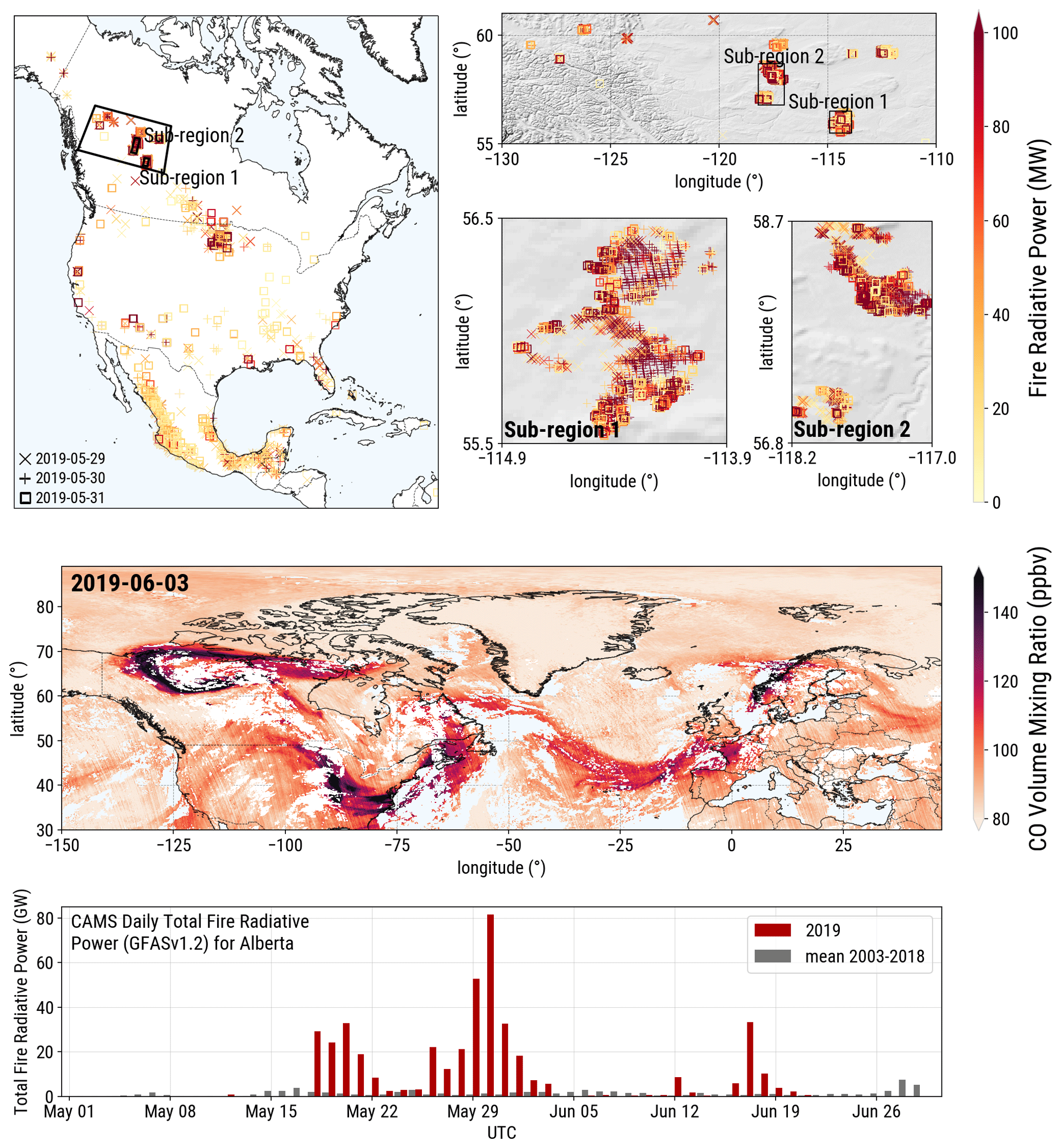
Figure 1 Overview of the Canadian wildfire event. Top: the fire radiative power on 29, 30, and 31 May 2019 are shown by different symbols. Middle: the TROPOMI observations of CO (carbon monoxide) on 3 June 2019. Bottom: CAMS daily total fire radiative power (GFASv1.2) for Alberta from May to June 2019, compared with the 2003–2018 mean daily total.

To define the exact locations and intensity of fires, the MODIS Collection 6 Level-2 active fire product was used (Giglio et al., 2016). The fire radiative power (FRP) observations from both Aqua and Terra satellites were considered. FRP describes the radiant energy released per time unit by burning, indicating the intensity of fires. Satellite-based carbon monoxide (CO) observations are a good proxy for assessing long-range transport of fire-related emissions. The TROPOMI (https://www.tropomi.eu/, last access: 22 August 2023) observations of CO on 3 June 2019, presented in Fig. 1, illustrate clearly that the emissions from the fires in Alberta were transported all the way to Europe.

The Alberta May 2019 wildfires have been used in many studies on newly developed methods for satellite-based applications of wildfire monitoring. Ban et al. (2020) and Zhang et al. (2021) developed machine-learning-based methods to monitor wildfire progression using spaceborne synthetic aperture radars and optical instruments. Both studies use the Alberta wildfires in their method evaluation. Furthermore, Tymstra et al. (2021) characterized the weather conditions for large Canadian spring wildfires including May 2019, whereas Whitman et al. (2022) studied the climate-related changes of wildfires in Alberta. Both Tymstra et al. (2021) and Whitman et al. (2022) concluded that climate change would make the wildfires larger and more intense in this region in the future.

2.2 Aerosol observations

2.2.1 CALIOP

The Cloud-Aerosol Lidar and Infrared Pathfinder Satellite Observation (CALIPSO) satellite (Winker et al., 2009, 2010) has been providing observations on aerosols and clouds since June 2006. CALIPSO carries the Cloud-Aerosol LIdar with Orthogonal Polarization (CALIOP) instrument, which measures the vertical structure of the atmosphere at two wavelengths: at 532 nm where it has two channels that are orthogonally polarized and at 1064 nm where it measures the total backscattered signal (Hunt et al., 2009).

In this study both the profile and layer products were utilized to locate smoke layers and estimate their optical properties. From CALIPSO lidar data, the Level 2 V4.20 product was used (which is the latest version of the data available at the time of data analyzing). The data were downloaded from the Atmospheric Sciences Data Center (ASDC), located at the National Aeronautics and Space Administration (NASA) Langley Research Center (LaRC). The CALIOP aerosol classification algorithms were used for the identification of the smoke layers. The CALIOP tropospheric aerosol subtype classification (Kim et al., 2018) uses integrated attenuated backscatter coefficient, depolarization ratio, surface type, altitude, and location to assign the layer to one of the following aerosol classes: clean continental, clean marine, dust, dusty marine, polluted continental/smoke, polluted dust, or elevated smoke (https://www-calipso.larc.nasa.gov/resources/calipso_users_guide/data_summaries/vfm/index_v420.php, last access: 22 August 2023). The depolarization ratio is enhanced if the particles are nonspherical; thus, it can be used to distinguish between, for example, dust and spherical aerosols.

In order to analyze only the most trustworthy observations, several quality control products were considered, and only nighttime measurements were used. The first criterion was that the cloud–aerosol discrimination (CAD) score had to be between −100 and −70, indicating high confidence of aerosol layers. Furthermore, only aerosol bins with the extinction quality control (QC) flags of 0, 1, 16, and 18 were used to ensure the good quality of the retrievals (Kim et al., 2018). In CALIOP observations, smoke particles can be classified as “polluted continental/smoke” or “elevated smoke”. In this study, only elevated smoke was considered since the focus is on fire-emitted aerosols. The separation between polluted continental and smoke aerosols is not possible in the polluted continental/smoke class.

2.2.2 Ground-based lidars and ceilometer

In order to evaluate the usability of CALIOP observations in the monitoring of aerosol mass in smoke plumes, we utilized open-access data from several ground-based lidar/ceilometer networks. The NASA Micro-Pulse Lidar Network (MPLNET) has been continuously providing aerosol and cloud properties, as well as the planetary boundary layer structures, at over 80 sites worldwide since 2000 (Welton et al., 2001). Currently, the observations from the polarized Micro-Pulse Lidar instruments are processed using the MPLNET Version 3 system (Welton et al., 2018). More information on MPLNET and data products is available on their website (https://mplnet.gsfc.nasa.gov, last access: 22 August 2023). For the European-based comparisons, besides MPLNET, observations submitted to the EU-funded Cloudnet project (Illingworth et al., 2007) and the polarization lidar network PollyNET (Baars et al., 2016) have been utilized. Cloudnet enumerates 17 permanent and numerous campaign stations across Europe, and observations are routinely collected, processed, visualized, and distributed through the ACTRIS Cloudnet data portal (http://cloudnet.fmi.fi, last access: 22 August 2023). PollyNET (https://polly.tropos.de/, last access: 22 August 2023) is utilizing the capabilities from multiwavelength polarization Raman lidars of type Polly (Althausen et al., 2009) to establish aerosol climatology. Observations from four stations were used in this study, which will be presented in Sect. 3.1: GSFC (NASA Goddard Space Flight Center) station (38.993^∘ N, 76.840^∘ W; 50 m a.m.s.l., Washington DC, USA) and Barcelona station (41.386^∘ N, 2.117^∘ E; 125 m a.m.s.l., Spain) of MPLNET; Granada station (37.164^∘ N, 3.605^∘ W; 680 m a.m.s.l., Spain), part of Cloudnet (Cazorla Cabrera and Alados-Arboledas, 2023); and Antikythera station (35.86^∘ N, 23.31^∘ E; 193 m a.m.s.l., Greece), member of PollyNET (Kampouri et al., 2021).

2.3 Models

2.3.1 MERRA-2 reanalysis aerosols

The Modern-Era Retrospective analysis for Research and Applications Version 2 (MERRA-2) is NASA's global reanalysis model (Gelaro et al., 2017). It includes meteorological variables, as well as aerosols and trace gases. MERRA-2 assimilates bias-corrected aerosol optical depth (AOD) at 550 nm from various sources, including satellite-based MODIS aerosol products (Buchard et al., 2017; Randles et al., 2017).

The spatial resolution of MERRA-2 is 0.5^∘ × 0.625^∘, and it has 72 pressure levels. MERRA-2 provides data with 1 or 3 h instantaneous or time-averaged time steps, depending on the variable, and data are available since 1980. In MERRA-2, aerosol output is written out every 3 h and it produces vertical profiles of mass mixing ratios for five different aerosol species: dust, sea salt, black carbon, organic carbon, and sulfate. The daily emissions of biomass burning used in MERRA-2 come from the Quick Fire Emission Dataset (QFED) version 2.4-r6 (Darmenov and da Silva, 2015) (after 2010). Based on the FRP, the QFED implements the cloud correction method from the Global Fire Assimilation System (GFAS; Kaiser et al., 2012) and applies a sophisticated treatment of emissions from non-observed land areas (Darmenov and da Silva, 2015).

In this study, we used the mass mixing ratios from the MERRA-2 assimilated aerosol mixing ratio data product inst3_3d_aer_Nv (GMAO, 2015a). We used linear interpolation of MERRA-2 aerosol profile data to spatially collocate the model data with CALIOP profiles. For temporal collocation, we used the nearest time step of the MERRA-2 aerosol data to match with CALIOP overpass.

2.3.2 CAMS reanalysis aerosols

The Copernicus Atmospheric Monitoring System (CAMS) Atmospheric Composition Reanalysis 4 (EAC4) is run by the European Centre for Medium-Range Weather Forecasts (ECMWF) (Inness et al., 2019). It consists of meteorological variables and also aerosol and trace gas information. The CAMS reanalysis assimilates total AOD observations, including satellite data from MODIS (Rémy et al., 2019). The spatial resolution of CAMS reanalysis data products is 0.75^∘ × 0.75^∘ with 60 model levels. The CAMS reanalysis provides aerosol data every 3 h, and data are available since 2003. The CAMS reanalysis provides vertical profiles of mass mixing ratios for five different aerosol species: organic matter, black carbon, sea salt, dust, and sulfate. Daily biomass burning emissions derive from the GFAS (Flemming et al., 2015, 2017), which is based on the combined MODIS observations of FRP from Terra and Aqua (Kaiser et al., 2012).

The collocation of CAMS reanalysis aerosol profiles was carried out similarly as for MERRA-2 – linear interpolation for spatial collocation and the closest time instant for temporal collocation.

Daily fire injection height information was available using the CAMS GFAS which assimilates FRP observations and meteorological conditions simulated from the ECMWF operational weather forecast. In particular, the daily injection height (mean altitude of maximum injection and altitude of plume top) is estimated by the Plume Rise Model (PRM) and IS4FIRES (Sofiev et al., 2012). The GFAS injection height calculations are not used in the reanalysis, but they were considered for the determination of the initial heights for the trajectories.

2.3.3 Trajectory model

In this study, we computed the air parcel trajectories using a custom Lagrangian trajectory model that moved the air parcels according to the MERRA-2 wind fields. The eastward and northward wind and vertical pressure velocity components from the MERRA-2 assimilated meteorological fields data product inst3_3d_asm_Nv were used (GMAO, 2015b). To get the wind components for the exact location and time of the air parcel, we linearly interpolated the MERRA-2 wind field information. We used a 5 min time step and simple forward Euler method in our trajectory computations. The vertical pressure level of the air parcel was converted to heights using MERRA-2 pressure profile information. In the trajectory model, the air parcels were restricted from going below the surface elevation. When reaching the surface elevation, the air parcels were moved along the wind components at the surface level. The trajectory model only computed the transport of the air parcels and did not simulate any other processes such as mixing, chemical transformation, or deposition of particles.

2.4 Methods

2.4.1 Estimation of mass from lidar signals

It is possible to estimate the particle mass concentration profile (m) from the vertical profile of lidar-derived backscatter coefficient (β), together with the particle mass density (ρ), the volume‐to‐extinction conversion factor (c_v), and the type-dependent lidar ratio (LR); see Eq. (1). The method described in Shang et al. (2021) was applied here to estimate the mass concentrations based on the measured backscatter coefficients at 532 nm or converted to 532 nm using the corresponding backscatter-related Ångström exponent (BAE); see Eq. (2).

$$\begin{array}{}\text{(1)}& {\displaystyle }m=\mathit{\rho }\cdot c_{\mathrm{v}}(\mathit{\lambda }=\mathrm{532})\cdot \mathit{\beta }(\mathit{\lambda }=\mathrm{532})\cdot \mathrm{LR}(\mathit{\lambda }=\mathrm{532}),\text{(2)}& {\displaystyle }\mathit{\beta }(\mathit{\lambda }=\mathrm{532})={\mathit{\beta }}_{\mathrm{meas}}(\mathit{\lambda }=\mathrm{1064})\cdot (\mathrm{532}/\mathrm{1064}{)}^{-\mathrm{BAE}}.\end{array}$$

The conversion factor at 532 nm of 0.16 ± 0.01 × 10⁻⁶ m for the fresh and medium-fresh smoke (i.e., less than 2 d) (or 0.13 ± 0.01 × 10⁻⁶ m for aged smoke) and a particle density of 1.3 g cm⁻³ were used for the biomass burning particles (Ansmann et al., 2021). Following Ansmann et al. (2021), we assume uncertainties of 10 % and 20 % in the conversion factor and smoke mass density. Using ground-based multiwavelength lidar measurements, the lidar ratio at 532 nm and the backscatter-related Ångström exponent between 532 and 1064 nm were derived as 71 ± 5 sr and 2.2 ± 0.3, respectively, for the smoke plumes during the same wildfire event as in this study (Shang et al., 2021). For the backscatter coefficient retrievals, we used relative uncertainties of 10 %, 15 %, and 25 % for ground-based lidar, ceilometer, and spaceborne lidar, respectively. These values were taken from Shang et al. (2021) and Ansmann et al. (2021). The Ångström value of 2.2 was applied to convert the ceilometer-measured backscatter coefficients at 1064 to 532 nm (Eq. 2), resulting in a relative uncertainty of 24 % on the converted backscatter coefficients. This study employed a lidar ratio at 532 nm of 70 sr, which was the value used for the aerosol subtype of elevated smoke in CALIOP version 4 (Kim et al., 2018). The lidar ratios at 532 nm for ground-based lidars are measured with a typical relative uncertainty of about 20 %, which can also be assumed for the 532 nm CALIOP lidar ratio for elevated smoke (the uncertainty is 70 ± 16 sr in CALIPSO V4 lidar data). More details of the uncertainties in the CALIPSO products can be found in Young et al. (2013, 2018). Applying the law of error propagation to Eq. (1) with the abovementioned uncertainties, we expected an overall uncertainty in the mass concentration estimates of 32 % for ground-based lidar and 40 % for ceilometer and CALIOP.

2.4.2 Selection of trajectories

There were 6480 trajectories generated, considered to be originated from a single day (0 to 24 h), from all initial heights (0 to 7.5 km), and from both wildfire sub-regions (nine initial spots in each, Fig. 1). The dominant air mass pathway was determined by the trajectory frequencies, which were calculated via the bivariate bin counts in two steps: the latitude and longitude trajectory frequencies were calculated based on 1^∘ × 1^∘ pixels, whereas the altitude and time trajectory frequencies were calculated based on 500 m × 1 h pixels. The pixels with an occurrence frequency above the median value were selected, referring to the most possible air mass transportation. Only the trajectories included in the predefined pixels were kept (less than 10 % of the total trajectories). These screened trajectories were used to define four-dimensional hypercubes, with a doubled resolution as previously used for the frequency pixels, considering the model uncertainties. Each hypercube has eight values of four variables (i.e., the edge values of latitude, longitude, altitude, and time). Next, the CALIOP-derived smoke layers (after the quality control; see Sect. 2.2.1) were automatically selected using these 4-D hypercubes to ensure that they are on the dominant air mass pathway. The uncertainties due to trajectory computations, wind data, and temporal and spatial collocation cause uncertainty in the estimates of the dominant air mass pathway. However, we estimate these uncertainties to be small and to not significantly affect the results of our study.

3 Results and discussion

3.1 Comparison of CALIOP retrievals with ground-based lidars and ceilometer

Among the automatically selected CALIOP smoke layers, four cases were intensively analyzed when nearby ground-based lidar/ceilometer observations were available.

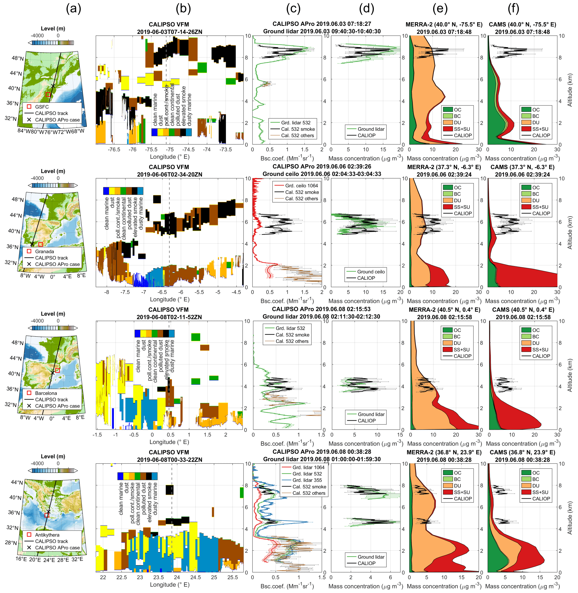
Figure 2 Comparison of vertical profiles of observations and simulations. Four sites with nearby CALIPSO overpasses, from top to down: GSFC (MPLNET), Washington DC, USA; Granada (Cloudnet), Spain; and Barcelona (MPLNET), Spain; Antikythera (PollyNET), Greece. (a) Ground-based site location, CALIPSO track, and selected CALIOP aerosol profile (APro) case location. (b) CALIPSO Level 2 Vertical Feature Mask (VFM) product with granule (yyyy-mm-ddTHH-MM-SS) given. (c) Backscatter coefficients at 532 nm from CALIOP (Cal.) Level-2 5 km APro product (corresponding to dashed line in panel b), with elevated smoke in black and other aerosol types in brown, uncertainties are given in gray. Backscatter coefficients from ground-based (Grd.) lidar or ceilometer at 532/1064/355 nm are also shown, with the time-averaging window given on the top. (d) Mass concentrations of the smoke layers, estimated from CALIOP or ground-based lidar/ceilometer. (e–f) Mass concentrations of different components (OC – organic carbon, BC – black carbon, DU – dust, SS – sea salt, SU – sulfate) from MERRA-2 or CAMS models.

Case 1: GSFC (MPLNET). On 3 June 2019, some lofted layers were detected by the ground-based lidar at GSFC station (https://mplnet.gsfc.nasa.gov/data?v=V3&s=GSFC&t=20190603, last access: 22 August 2023). Version 3 Level 1.5 aerosol data are only available after 09:40 UTC after the quality control. The closest CALIPSO track was passed at about 07:18 UTC. From the CALIPSO VFM (Vertical Feature Mask) product (Fig. 2, first row, panel b), elevated smoke layers were detected at about 7–10 km for longitudes from −75.5 to −74.5^∘ E, whereas dust layers were identified below at about 6 km. These two layers were also detected by the ground-based lidar (Fig. 2, first row, panel c). Particle backscatter coefficient of the smoke layer derived from the ground-based lidar is slightly higher than the one from CALIOP. Consequently, the layer mean mass derived from the ground-based lidar is 30 % higher than the CALIOP estimate. The MPLNET and CALIOP layer mean masses are 12.2 ± 4.5 and 8.5 ± 4.6 µg m⁻³, respectively. Note that there is about 2.5 h difference between these two observations; thus, the observed smoke layers could be from different parts of the plume.

Case 2: Granada (Cloudnet). On 6 June continuous lofted layers were detected by CALIOP for longitudes from −7 to −4.5^∘ E and for altitudes 5–8 km (Fig. 2, second row, panel b). CALIPSO classified these layers as elevated smoke or polluted dust. Faint lofted layers were also visible in the morning from the near-real-time non-screened attenuated backscatter coefficients of the CHM15k ceilometer at Granada (https://cloudnet.fmi.fi/file/155df385-c4b1-4cd0-b746-bab2afb31355, last access: 22 August 2023). The smoke layer (at ∼ 5 to 7 km) was well detected by both instruments with a good agreement (Fig. 2, second row, panel c). The ceilometer-derived backscatter coefficients (1 h time-averaged centered on the CALIOP profile) of the smoke layer measured at 1064 nm were used to estimate the layer mass concentrations following the method presented in Sect. 2.4.1, resulting in a layer-mean value of 6.6 ± 3.7 µg m⁻³ compared to 8.3 ± 3.0 µg m⁻³ from CALIOP. Thus, in this comparison the CALIOP retrieval produces 26 % larger aerosol mass for the smoke layer.

Case 3: Barcelona (MPLNET). Only two smoke layers were identified by the CALIPSO on 8 June for the selected sector (Fig. 2, third row, panel b). The one closer to the Barcelona station was selected in this section, ranging from about 3.5–5 km (a CALIOP horizontal averaging of 20 km was applied). The CALIOP ALay products of this smoke layer show an AOD of ∼ 0.05 and an estimated particulate depolarization ratio of ∼ 0.02 at 532 nm. Several layers up to 6 km were detected in the morning on that day by the ground-based lidar at Barcelona station (https://mplnet.gsfc.nasa.gov/data?v=V3&s=Barcelona&t=20190608, last access: 22 August 2023). The atmosphere was quite inhomogeneous; thus, 1 min ground-based lidar profiles were used to compare with CALIOP-derived backscatter coefficient (Fig. 2, third row, panel c), showing lower values in the smoke layer. Due to the lower backscatter coefficient, the ground-based estimate for layer mean mass (4.4 ± 1.6 µg m⁻³) is 43 % smaller than the CALIOP estimate (6.3 ± 2.1 µg m⁻³). The ground-based lidar-derived particle depolarization ratio of this layer is ∼ 0.03 ± 0.01. There is a 4 min difference between the two measurements.

Case 4: Antikythera (PollyNET). Faint smoke layers were identified by CALIOP for the considered sector on 8 June (Fig. 2, fourth row, panel b). The horizontal resolutions of 80 km were required to detect these layers due to the small aerosol amount. The ground-based lidar at PANGEA observatory in Antikythera also observed the lofted layers (https://polly.tropos.de/datavis/location/38/19/1?dates=[2019-06-08T00:00:00,2019-06-09T00:00:00], last access: 22 August 2023). The backscatter coefficients derived from the ground-based lidar (1 h time-averaged) and CALIOP show good consistency (Fig. 2, fourth row, panel c), with about half an hour time difference. Two smoke layers were located at about 4.5 and 7.5 km, having AODs at 532 nm of about 0.017 and 0.014, respectively, and estimated particulate depolarization ratios of ∼ 0.06 (CALIOP ALay products). The ground-based lidar observed a thicker layer compared to CALIOP for the upper one. Some of the layers could not be fully detected by CALIOP, e.g., the thin aerosol layers with low concentrations, as well as the boarders of layers where there are fewer aerosols. The estimate for the layer mean mass from the ground-based lidar (4.1 ± 1.3 µg m⁻³) is 12 % larger than the CALIOP-retrieved estimate (3.6 ± 1.3 µg m⁻³). Good agreements were also found for the aerosols inside the boundary layer (i.e., below 3 km), which were classified as dust and dusty marine by CALIOP.

3.2 Analysis of the Alberta plume event

During the wildfire event, highest fire emissions were detected on 29–31 May (Fig. 1). Following the method described in Sect. 2.4.2, the CALIOP smoke layers on the dominant air mass pathway originating from the same day were automatically selected. Their location and time–height information are shown in Fig. 3. In total, 1336 smoke layers were selected, related to 1194 CALIOP 5 km profiles. Considering the different horizontal averaging lengths applied in the CALIOP detection scheme, there are 259 unique detections, among which the layer numbers with horizontal averaging of 5, 20, and 80 km are 75, 417, and 844, respectively. The largest number of auto-selected layers was found to be originating from 29 May; thus, more intense investigation was performed for these layers, and the trajectory frequencies from 29 May were used as the colored background in Fig. 3. Smoke layers observed on the same day were grouped, and were related to the age of the smoke particles, for the illustration of the evolution of the particle properties during the transportation (Fig. 4). The CALIPSO Level-2 5 km aerosol layer (ALay) products are used here. Note that the optical depths were summed up (denoted as AOD here) in case there are several smoke layers detected in the same profile (Fig. 4a). In the ALay product, aerosol layers are detected using a “nested multigrid averaging scheme” (Vaughan et al., 2009), which may produce vertically overlapping layers. In such cases, CALIPSO Level-2 5 km aerosol profile (APro) products were used instead to calculate the AODs. The same method was also applied later for the column mass calculations to avoid the layer overlapping issue. A clear tendency of AOD and mass decreasing can be seen in Fig. 4a–b. The median values of AOD (or layer-mean mass concentration) decreased from 0.25 (56 µg m⁻³) for the fresh smoke (∼ 1 d aged) to 0.013 (4.5 µg m⁻³) for the aged smoke after the long-range transportation (∼ 10 d aged). The higher decreasing rate was found at the beginning of transportation. Slight increases in AODs and mass concentrations were observed in the middle of the transportation over ocean; these smoke layers were probably a mixture of smoke particles originating from several fire source days (as shown by overlapped symbols in Fig. 3, e.g., CALIPSO track 06-02T04-57). Taylor et al. (2014) reported the mass concentrations of organic aerosol and black carbon to be in the same range for smoke plumes of ∼ 1–2 d after passing over the fires source, unaffected by the wet deposition (precipitation). The estimated particulate depolarization ratio at 532 nm of the smoke layers slightly increased during the transportation, with median values from 0.03 to 0.06 (Fig. 4c). There is no clear tendency for the relative humidity (Fig. 4d). A decreasing tendency was also found for the total attenuated backscatter color ratio (the ratio of attenuated backscatters at 1064 and 532 nm), which is an independent quantity not being used in the subtyping algorithm in the troposphere (Omar et al., 2009). Nevertheless, this parameter is modulated by the scattering ratio and is therefore not a direct indicator of particle size. No clear tendency was found for the particulate backscatter color ratio. Smoke layer altitudes were increased at the beginning, then they split into two air mass pathways (e.g., on 1 June). Layer heights decreased a bit over the oceans, then they climbed again over Europe (Fig. 3). The depths of these smoke layers range from 0.30 to 1.44 km with a mean value of 0.68 ± 0.26 km.

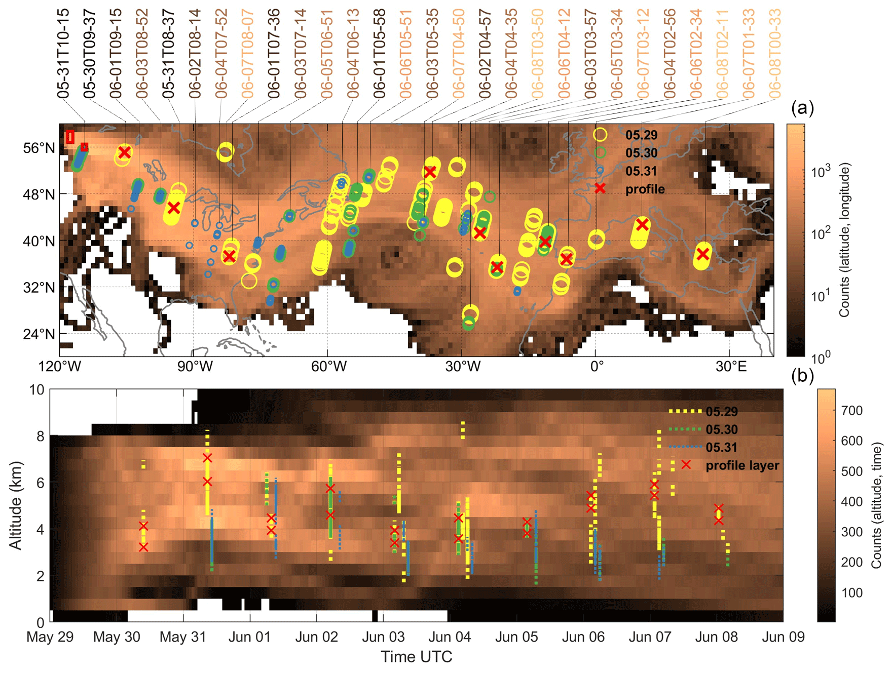
Figure 3 Trajectory frequency plots (29 May as source) with automatically selected CALIOP smoke layers (from fire sources originating on 29, 30, or 31 May shown by circles (top) and dashed lines (bottom) with different colors and sizes). The corresponding CALIPSO granule information is given as “mm-ddTHH-MM” on the top, with color scales showing from earlier (darker) to later (lighter) dates. Red cross: CALIOP APro profile cases used in Fig. 5. Two sub-regions of fire source areas are given in red rectangles on the top-left in the top figure.

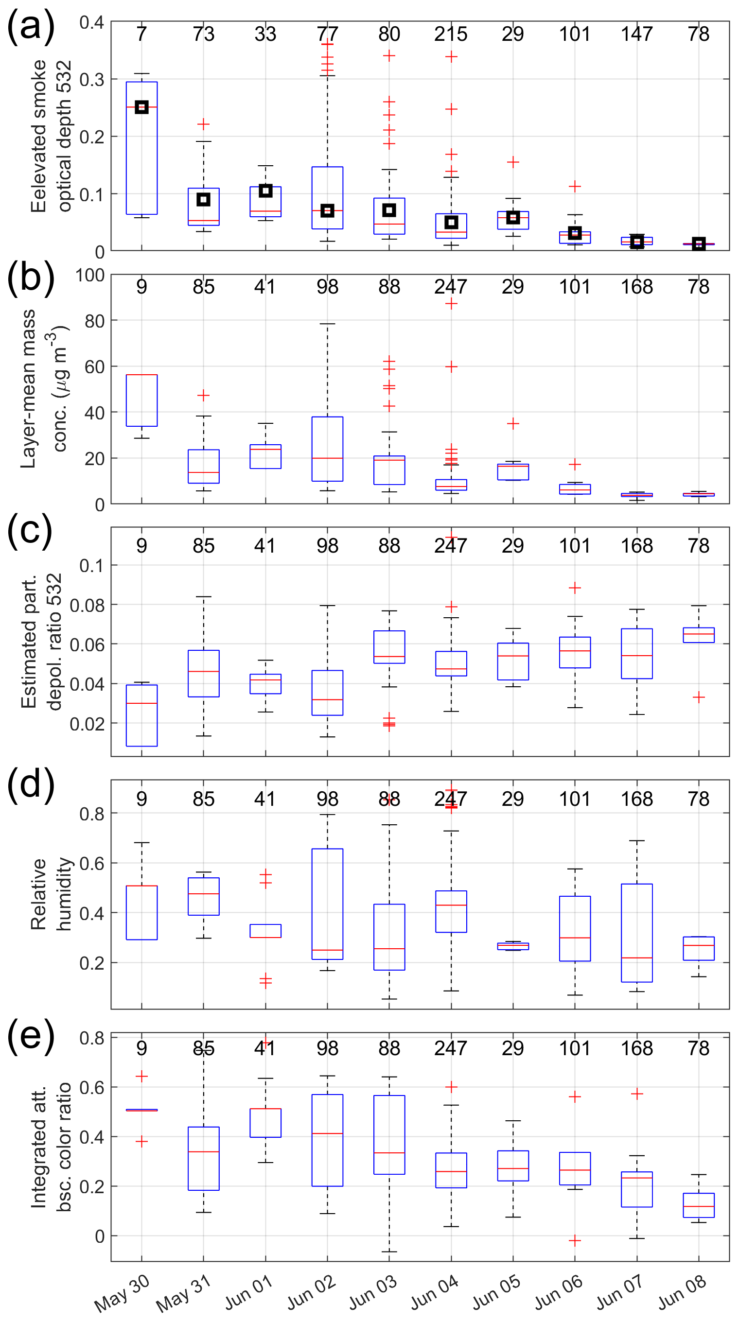
Figure 4 Statistical properties of smoke layers originating from the Alberta plume event on 29 May 2019. CALIPSO Level-2 5 km ALay products were used. In case of overlapping layers in the vertical, 5 km APro products were used to calculate the AODs. Used layer numbers (or profile numbers in panel a) in each boxplot are given on the top. AODs of the smoke layers used in Fig. 5 are shown as black squares in panel (a).

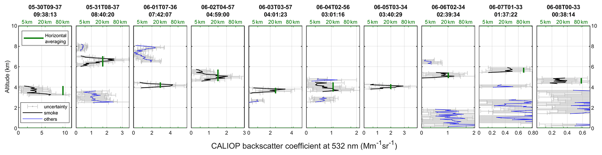
Figure 5 Profile examples. One profile was selected each day (only originated from one day source). CALIPSO Level-2 5 km APro products were used. The CALIPSO granule and profile time are given on top. Backscatter coefficients of the elevated smoke type (or other aerosol types) are shown in black (or blue), with the uncertainties given in gray. The horizontal averaging applied is in green.

For better illustration, one profile from the CALIPSO APro products was selected on each day so as to present the time evolution using the vertical profiles of backscatter coefficients (Fig. 5). The profile locations are given in Fig. 3, whereas the smoke layer AODs are given in Fig. 4a. The CALIPSO algorithm applied different horizontal averaging regarding the signal-to-noise ratio of the aerosol layer.

3.3 Comparison of observed and simulated smoke layers

As was discussed in Sect. 3.1 and shown in Fig. 2, mass retrievals from CALIOP have overlapping error bars in all cases with ground-based lidar/ceilometer retrievals; in three cases, the CALIOP means lie within the ground-based error bars and vice versa. To evaluate if models could also capture these plumes, the CALIOP retrievals were compared with aerosol mass concentration profiles from the reanalysis models MERRA-2 and CAMS. These comparisons are presented in Fig. 2e and f. Based on these case studies, MERRA-2 appears to have higher aerosol concentrations than CAMS at the altitudes of the smoke layers. Consequently, MERRA-2 seems to agree better with the CALIOP mass retrievals. However, when the contribution of different aerosol types is considered, it is clear that MERRA-2 produces more comparable aerosol concentrations because it is overestimating the contribution of dust. Recently, Li et al. (2023) reported a quantitative evaluation analysis, showing that the dust products from MERRA-2 reanalysis have higher column concentrations than the satellite-based component retrievals, with relative differences of about 20 % to 70 %. The comparison at GSFC implies that CAMS is better at simulating lofted smoke layers near the source regions as it includes elevated OC concentrations at higher altitudes. However, the elevated OC concentrations are located between 1 and 8 km, whereas the CALIOP retrieval shows that the smoke plume was mainly above 8 km. Overall, these case studies indicate that reanalysis models have difficulties in capturing the location and properties of long-range-transported smoke. In fact, the difficulties in representing the aerosol altitude is generally true of most models, as stated in Das et al. (2017), Zhong et al. (2022), and references therein.

In order to obtain a more complete picture of the performance of these models, a comparison using all the smoke layers within the transported plume was carried out. As a first step, the total column was considered. The CALIOP profiles with the presence of layers which did not fulfill the QC were excluded, reducing the profile number to 622.

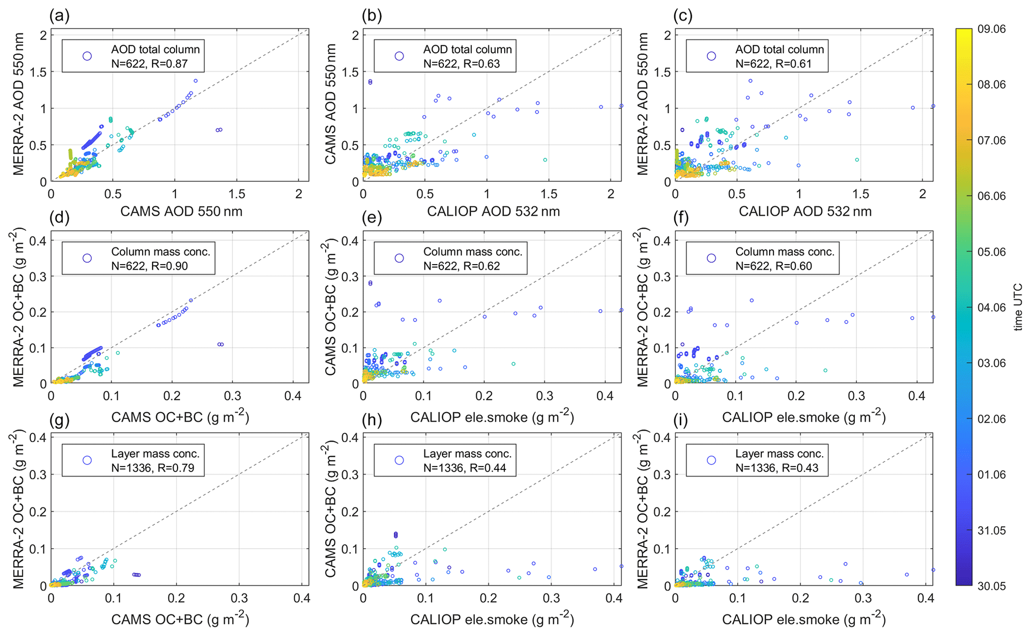
Figure 6 Comparison of observed and simulated products for locations where CALIOP detected smoke layers; (a–c) total column AOD (tropospheric AODs from CALIOP); (d–f) column mass concentration of black carbon (BC) and organic carbon (OC) of CAMS and MERRA-2, and summed layer mass concentration of CALIOP elevated smoke layers; (g–i) layer mass concentrations of CALIOP elevated smoke layers and layer mass concentrations (three times the depth of the CALIOP layers) of BC and OC of CAMS and MERRA-2.

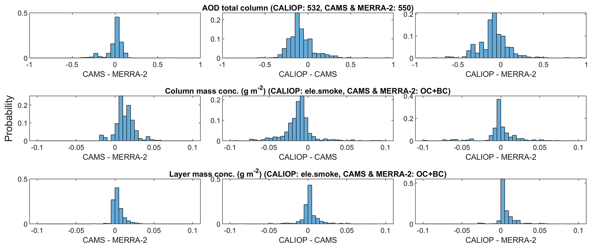
Figure 7 Similar with Fig. 6 but shown by histograms of the differences of observed and simulated products.

Simulated and observed total column AODs were compared with each other. The CALIOP AOD is calculated only from tropospheric aerosols and based on the analysis of CALIOP aerosol layer and profile products, as the stratospheric contribution is insignificant during the studied cases. These comparisons are presented in the first row of Fig. 6 as scatterplots and of Fig. 7 as the histograms of the differences. CAMS and MERRA-2 exhibit good agreement with their AOD values. However, when compared with the CALIOP observations, clear differences emerge. CALIOP AODs tend to be smaller than the simulated values; even though the values are positively correlated, there is significant variability. Consequently, the correlation coefficients are only 0.63 and 0.61 for CAMS and MERRA-2, respectively. The fact that bias in reanalysis AOD is unavoidable must be noted, as stated by several studies (Mukkavilli et al., 2019; Song et al., 2018; Salamalikis et al., 2021; Gueymard and Yang, 2020). Furthermore, some aerosol layers could not be fully detected by CALIOP due to the weak signal-to-noise ratio as discussed in Sect. 3.1 and in Thorsen et al. (2017).

The column mass concentrations of smoke were also compared, shown as the second row in Figs. 6 and 7. The CALIOP elevated smoke layers were combined in each profile to estimate the smoke mass concentrations. Furthermore, only OC and BC masses were considered in the calculation of the simulated smoke masses. High correlation was found for the simulated smoke column mass concentrations for CAMS and MERRA-2. However, CAMS simulated higher smoke concentrations than MERRA-2. When compared with CALIOP products, the correlation coefficients are quite similar as the ones for AODs, demonstrating that the smoke aerosols are dominant in the column. These column smoke mass concentrations were also presented in Fig. 8 to illustrate the smoke transportation. Mass burden decrease can be clearly seen from west (closer to the source) to east (far from the source), corresponding to the fresh-to-old-aged smoke particles. The models exhibit a clearer contrast between the continents than CALIOP, which indicates that the smoke aerosols in the models could be removed too efficiently.

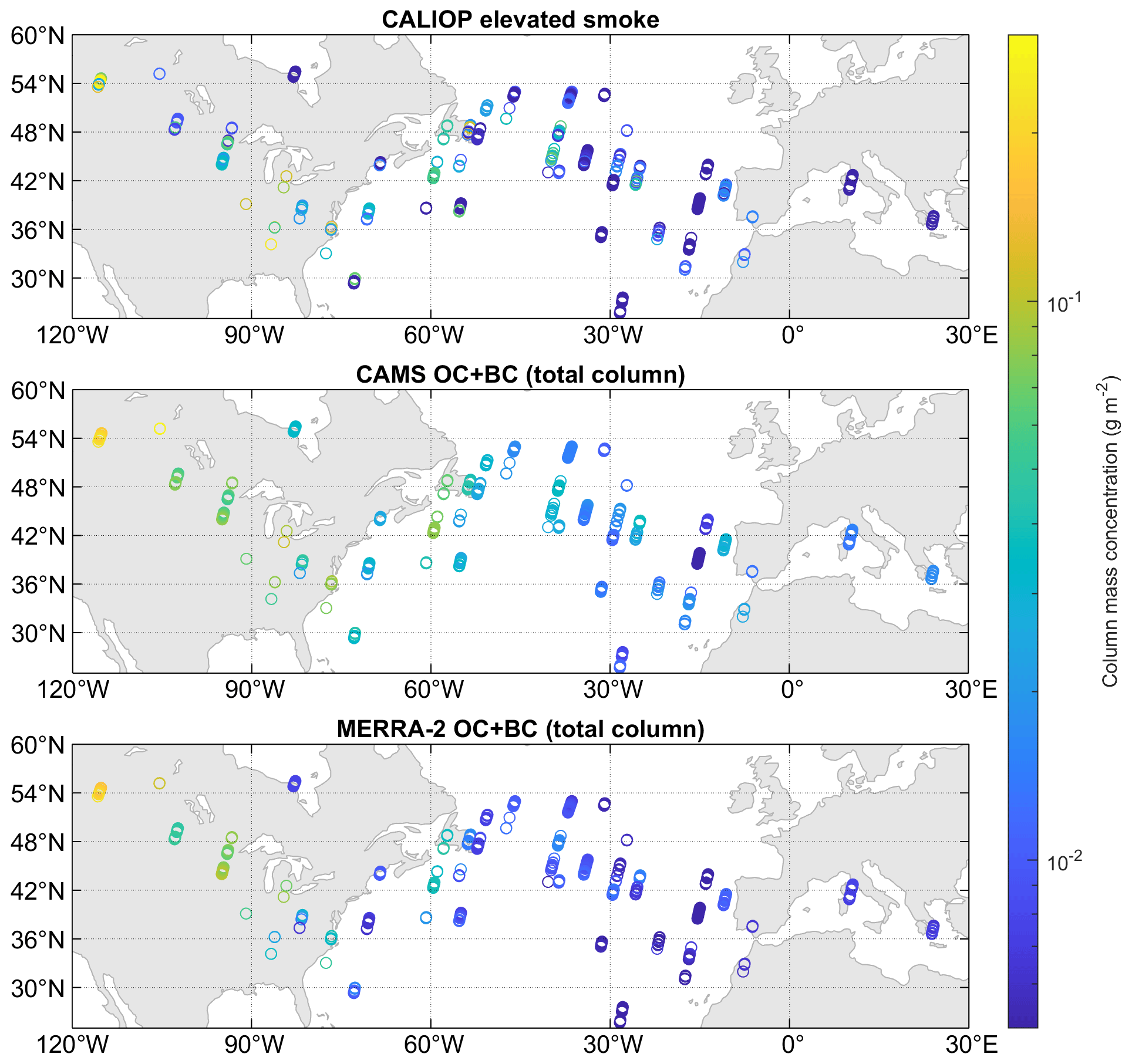
Figure 8 Column mass concentrations of smoke using CALIOP elevated smoke layers, black carbon (BC), and organic carbon (OC) from CAMS, as well as BC and OC from MERRA-2.

The accuracy of the simulated smoke layers was compared in a similar fashion using the integrated aerosol mass of the layers. As the models might have the smoke layers at slightly different altitudes than in the observations, the collocation criteria were relaxed by assuming that the thickness of the simulated layer was 3 times larger than in the observations. As an example, if CALIOP had observed a 1 km thick smoke layer at the altitude of 4 km, the simulated layer was assumed to be centered at the same altitude but its thickness was set to be 3 km. These comparisons are presented as the third row in Figs. 6 and 7. In this comparison, the models do not agree so well with each other. Moreover, the modeled concentrations are lower than the CALIOP-based concentrations. These results highlight the difficulty in simulating biomass burning plumes: both of these reanalysis models have difficulties in reproducing the location, altitude, layer depth, and aerosol concentration of the plumes.

4 Conclusions

In May and June 2019, smoke plumes from Canadian wildfires were advected all the way (across North America and the North Atlantic) to Europe. To analyze the evolution of the plumes and to estimate the amount of smoke aerosols transported to Europe, retrievals from the spaceborne lidar CALIOP were used. Mass retrievals from CALIOP were in good agreement with retrievals from ground-based lidars, independently from the distance to the source. Over North America, the CALIOP layer mean mass concentration was 30 % smaller than the ground-based estimate (with about 2.5 h time gap), whereas over southern Europe that difference varied between 12 % and 43 %. These comparisons indicate that CALIOP data, as well as current (e.g., DQ2 of CNSA; Dai et al., 2023; https://www.cnsa.gov.cn/, last access: 22 August 2023) and upcoming (e.g., EarthCARE, https://earth.esa.int/eogateway/missions/earthcare, last access: 22 August 2023; Aeolus-2, https://www.esa.int/ESA_Multimedia/Images/2022/10/Aeolus-2_Value_of_Information, last access: 22 August 2023; AOS, https://aos.gsfc.nasa.gov/home.htm, last access: 22 August 2023) satellite missions with the capability to provide lidar measurements of backscatter coefficient and depolarization ratio, could be used to estimate aerosol masses in remote regions where ground-based observations are not available.

The analysis of aerosol mass concentrations over North America and Europe showed that less than one-tenth of the emitted mass survived the transport over the Atlantic Ocean. This information is valuable for evaluating transport efficiency in atmospheric models. The comparisons with reanalysis models MERRA-2 and CAMS showed that both models have difficulties in representing the aerosol mass of the studied smoke plumes, especially when the aerosol composition is taken into account. For example, the aerosol mass profiles in MERRA-2 matched quite well with the smoke layers observed with CALIOP, but most of the mass in the simulation originated from dust not organic or black carbon as one would expect for smoke plumes. Consequently, reanalysis simulations should be taken cautiously in the analysis of long-range-transported smoke in the boreal region.

These findings indicate that in order to estimate the transport and deposition of smoke aerosols to remote and pristine regions, high-quality observations are still needed. Passive satellite instruments can provide extensive spatial coverage, but they are incapable of accurately providing the altitude of the elevated plumes, and their accuracy starts to suffer over polar regions because of non-optimal measurement geometry. Spaceborne lidars are limited in spatial coverage, but the coverage improves closer to the poles. Furthermore, lidars can provide information on the vertical location and extent of the aerosol plumes, which is invaluable for impact studies and model development. The increasing wildfire activity produces a complicated global layering of smoke subtypes (fresh to aged), with emitted plumes from various stages from the burning phase (which impact the emissions). Even within the category of “smoke”, the properties of the aerosols can vary widely, especially when they linger in the Northern Hemisphere for weeks to months. Besides, other aerosols may also be mixed in the smoke plumes. For example, the Raikoke volcanic eruption in 2019 occurred only about 2 weeks after the Alberta plume event analyzed in this study; mixtures of smoke and volcanic plumes were present in the atmosphere for many weeks. These increasingly complex problems affect nearly the entire Northern Hemisphere every year. That demonstrates the need to continue deploying spaceborne lidars and ground-based lidar and ceilometer networks, especially those with enhanced capabilities which provide more accurate results and the ability to retrieve microphysical properties of the layers. As the CALIPSO science mission ended on 1 August 2023, there currently is an observational gap during the absence of the upcoming spaceborne lidar missions. This study points to the urgent need for future lidar missions in space, as well as the need of near real-time open-access provision of spaceborne lidar measurements. In addition, it would be good to study in the future how operational aerosol forecasts rather than reanalyses perform for long-range transport, including for the boreal regions and the Arctic.