the Creative Commons Attribution 4.0 License.
the Creative Commons Attribution 4.0 License.
 | 29 Jan 2024
Aerosol-related effects on the occurrence of heterogeneous ice formation over Lauder, New Zealand ∕ Aotearoa
Patric Seifert
J. Ben Liley
Martin Radenz
Osamu Uchino
Isamu Morino
Tetsu Sakai
Tomohiro Nagai
Albert Ansmann
The presented study investigates the efficiency of heterogeneous ice formation in natural clouds over Lauder, New Zealand / Aotearoa. Aerosol conditions in the middle troposphere above Lauder are subject to huge contrasts. Clean, pristine air masses from Antarctica and the Southern Ocean arrive under southerly flow conditions, while high aerosol loads can occur when air masses are advected from nearby Australia. This study assesses how these contrasts in aerosol load affect the ice formation efficiency in stratiform midlevel clouds in the heterogeneous freezing range (−40 to 0 ∘C). For this purpose, an 11-year dataset was analyzed from a dual-wavelength polarization lidar system operated by National Institute of Water and Atmospheric Research (NIWA), Taihoro Nukurangi, at Lauder in collaboration with the National Institute for Environmental Studies in Japan and the Meteorological Research Institute of the Japan Meteorological Agency. These data were used to investigate the efficiency of heterogeneous ice formation in clouds over the site as a function of cloud-top temperature as in previous studies at other locations. The Lauder cloud dataset was put into context with lidar studies from contrasting regions such as Germany and southern Chile. The ice formation efficiency found at Lauder is lower than in polluted midlatitudes (i.e., Germany) but higher than, for example, in southern Chile. Both Lauder and southern Chile are subject to generally low free-tropospheric aerosol loads, which suggests that the low ice formation efficiency at these two sites is related to low ice-nucleating-particle (INP) concentrations. However, Lauder sees episodes of continental aerosol, more than southern Chile does, which seems to lead to the moderately increased ice formation efficiency. Trajectory-based tools and aerosol model reanalyses are used to relate this cloud dataset to the aerosol load and the air mass sources. Both analyses point clearly to higher ice formation efficiency for clouds which are more strongly influenced by continental aerosol and to lower ice formation efficiency for clouds which are more influenced by Antarctic/marine aerosol and air masses.
- Article
(5410 KB) - Full-text XML
- BibTeX
- EndNote


Comprehension of cloud formation and cloud lifecycle is essential for adequately describing the Earth's climate system (Stephens, 2005). An important step towards such understanding lies in disentangling and eventually quantifying the complex processes of aerosol–cloud interaction (Lohmann and Feichter, 2005). Aerosol particles are required in the formation of liquid droplets and ice crystals from vapor phase by acting as cloud condensation nuclei (CCN) and as ice-nucleating particles (INPs) in the heterogeneous freezing temperature range from approximately −40 to 0 ∘C, respectively. In this temperature range, mixed-phase clouds can exist. They are of special interest in current atmospheric research because they can lead to both cooling or warming at Earth's surface (Sun and Shine, 1994; Hogan et al., 2003; Shupe and Intrieri, 2004; Zuidema et al., 2005) and because of their critical role for precipitation (Korolev et al., 2017).
In observational studies, it is difficult to separate thermodynamical, dynamical, and aerosol-related effects on cloud microphysics. Dynamics and thermodynamics are considered to preside over aerosol-related effects on cloud microphysical properties. Nevertheless, significant influence of aerosol conditions on cloud properties, cloud evolution, and precipitation has been confirmed in observational and modeling studies (Seifert et al., 2012; Possner et al., 2017; Solomon et al., 2018; Zhang et al., 2018; Desai et al., 2019).
The strong contrast in aerosol particle load and composition between the Southern Hemisphere and Northern Hemisphere midlatitudes (Tegen et al., 1997) can therefore be expected to lead, as well, to differences in cloud abundance and cloud properties in those regions. Indeed, the recurrent abundance of supercooled liquid cloud layers over the Southern Ocean (Hu et al., 2010; Tan et al., 2014; Huang et al., 2015) has a sensitive impact on the energy balance of this area (Trenberth and Fasullo, 2010; Bodas-Salcedo et al., 2014, 2016, 2019). These regional differences in the occurrence of supercooled liquid clouds might be caused by the lack of INPs in the largely pristine Southern Ocean (Hamilton et al., 2014). Shipborne INP measurements presented by Welti et al. (2020) and McCluskey et al. (2018a) confirm the rareness of INPs in the Southern Ocean. Tatzelt et al. (2022), also from shipborne INP measurements, conclude based on correlation between aerosol physicochemical properties and proxies of biological activity in the ocean as well as backward-trajectory analyses that indications for local INP sources are rare. Therefore, Tatzelt et al. (2022) interpret the INP populations as mixed long-range-transported biogenic and mineral dust INP from coastal or terrestrial sources which are sparse and distant (Vergara-Temprado et al., 2017).
On the other hand, marine organic aerosol is considered to be potentially an important source of INPs, especially over remote oceanic regions such as the Southern Ocean (Wilson et al., 2015; DeMott et al., 2016). By introducing marine organic aerosol into an Earth system model via a physically based parameterization instead of empirical proxies of biological activity, Zhao et al. (2021) concluded that marine INP dominate primary ice nucleation in the Southern Ocean at pressure levels above 400 hPa. McCluskey et al. (2019) compared shipborne INP measurements with model representations and found sea spray aerosol as the dominant contributor to primary ice nucleation in the Southern Ocean, though, also stressing the potential role of long-range-transported mineral dust and the need for modeling and observational studies on vertical and seasonal variability in INP and aerosol composition over remote regions.
The representation of the abovementioned contrasts in weather and climate models may impact these model's performance. Coupled Model Intercomparison Project (CMIP) models consistently showed and still show a positive bias in the absorbed shortwave radiation over the Southern Ocean (Trenberth and Fasullo, 2010; Grise et al., 2015; Zelinka et al., 2020; Varma et al., 2020; Kajtar et al., 2021; Schuddeboom and McDonald, 2021). This is largely attributed to simulating too much ice in Southern Ocean clouds compared to observations, which is another common bias in CMIP models (Kuma et al., 2023). A reduced frequency of liquid clouds leads to too less reflected shortwave radiation. This leads to an enhanced heating at the surface, which in turn causes a too large ocean heat uptake (Franklin et al., 2013; Hyder et al., 2018). The reasons for these observed differences and widespread model biases remain partly unresolved and therefore disputed, but hemispheric contrasts in aerosol load and type, including the low abundance of INPs from terrestrial sources, in combination with atmospheric dynamics, are suspected to play a role (Radenz et al., 2021a).
Mallet et al. (2023) and Humphries et al. (2023) highlight the heterogeneity of the pristine Southern Ocean region and suggest coordinated, long-term, and contrasting observational studies for validating and improving the models. Already, Minikin et al. (2003) performed aircraft in situ measurements over the Northern Atlantic and Southern Ocean and found a factor of 2–3 lower aerosol concentration in the free troposphere over the latter compared to over the former. Gayet et al. (2004) used the same measurements, focusing on cirrus evolution and properties, and derived lower cirrus ice crystal number concentrations in the southern than in the northern midlatitudes. Using spaceborne polarization lidar, Choi et al. (2010) demonstrated a negative correlation of supercooled cloud fraction with dust aerosol frequency. However, Mace et al. (2021a) used ship-based lidar observations (Mace et al., 2021b; McFarquhar et al., 2021) to underline that such spaceborne lidar phase statistics of mixed-phase clouds have a low bias in mixed-phase cloud occurrence over the Southern Ocean. To try to overcome spaceborne lidar observation and detection limits, Villanueva et al. (2020) used spaceborne observations in combination with aerosol reanalysis and found cloud glaciation to be differently susceptible to otherwise similar dust loads in the Southern Hemisphere compared to the Northern Hemisphere, which they found to agree with other findings on hemispheric differences in the mineralogical composition and related freezing efficiency of dust.
In the Southern Hemisphere midlatitudes, ground-based lidar was first used by Kanitz et al. (2011) to assess the thermodynamic phase of stratiform mixed-phase clouds observed over Punta Arenas, Chile. They found 50 % of clouds glaciated at −30 ∘C, compared to the same glaciation occurring already at −13 ∘C in the Northern Hemisphere midlatitudes (Seifert et al., 2010). Alexander and Protat (2018) corroborated these results in a similar study performed with lidar data from Kennaook / Cape Grim. Radenz et al. (2021a) performed a contrasting study using a longer-term dataset (than Kanitz et al., 2011) again from clean and pristine Punta Arenas but also including Doppler wind lidar and Doppler cloud radar, from dust-laden Eastern Mediterranean (Limassol, Cyprus), and from polluted northern midlatitudes (Leipzig, Germany). They found the ice formation efficiency for clouds observed over Punta Arenas to be most strongly suppressed compared to Leipzig and Limassol for clouds decoupled from the surface aerosol reservoir. Therefore, Radenz et al. (2021a) emphasize, besides the impact of gravity waves, the importance of quantifying terrestrial INP sources in the Southern Ocean. These terrestrial emissions need to be quantified by observations of free tropospheric aerosol up- and downwind of major landmasses in order to identify regions where cloud microphysics are most strongly impacted by these INPs (Radenz et al., 2021a).
This is strong motivation to extend such investigations of aerosol effects on mixed-phase clouds to New Zealand / Aotearoa. There, besides clean marine conditions, episodic aerosol transport from Australia (wildfire smoke, desert dust, urban haze) is occurring (Liley et al., 2001; Jones et al., 2001; Liley and Forgan, 2009). This enables a unique contrasting study at a single location which would not be possible in the permanently polluted Northern Hemisphere midlatitudes or in the permanently clean environment (of the free troposphere) of, for example, Punta Arenas. To investigate the efficiency of heterogeneous ice formation in natural clouds, this study makes use of a dataset which is unparalleled in the Southern Hemisphere, consisting of long-term ground-based polarization lidar measurements on the South Island /Te Waipounamu of New Zealand.
The paper is structured as follows. In Sect. 2, the used data and methods are introduced. In Sect. 3, first, a measurement example is described as a case study (Sect. 3.1). Later, general air mass statistics based on trajectory and aerosol model reanalysis are provided (Sect. 3.2). The retrieved cloud statistics are then presented in Sect. 3.3. In Sect. 3.4, the separation of clouds based on the air mass statistics is presented. Finally, in Sect. 4, the findings are summarized and an outlook is provided.
2.1 Lauder lidar system
Since 1992, lidar observations have been conducted by the National Institute of Water and Atmospheric Research (NIWA), Taihoro Nukurangi, at the Lauder Atmospheric Research Station on the South Island / Te Waipounamu of New Zealand, in collaboration with the Meteorological Research Institute of the Japan Meteorological Agency (MRI/JMA) (Uchino et al., 1995). In February 2009, the lidar system was upgraded with polarization capability (Nagai et al., 2010). After this upgrade, lidar observations are conducted by NIWA in collaboration with the National Institute for Environmental Studies (NIES) in Japan and MRI/JMA. The detailed specifications of the zenith-pointing dual-wavelength (1064, 532 nm) polarization lidar system are described in Nakamae et al. (2014) and Sakai et al. (2016). It uses a Nd:YAG (neodymium-doped yttrium aluminum garnet) laser with a pulse energy of 150 mJ, a pulse width of 5 ns, and a repetition rate of 10 Hz. The telescope diameter is 30.5 cm, and the range resolution is 7.5 m. The field of view is 1 mrad, and the beam divergence is 0.2 mrad. The signal at 1064 nm wavelength is detected with an analogue-mode avalanche photodiode, and two polarization components of the signals at 532 nm wavelength are detected with three photomultiplier tubes. This allows for the retrieval of the particle backscatter coefficient at 532 nm and 1064 nm wavelength using the Klett–Fernald–Sasano algorithm (Klett, 1981, 1985; Fernald, 1984; Sasano et al., 1985), as well as the particle depolarization ratio at 532 nm wavelength. Lauder Atmospheric Research Station is located at 370 ; 45.037∘ S, 169.683∘ E. For this study, an 11-year polarization lidar dataset from 15 March 2009 to 5 April 2020, particularly the co- and cross-polarized signals at 532 nm wavelength, was used.
2.2 Identification of cloud layers and their phase
The cloud layers observed by polarization lidar were classified as either ice-containing or pure liquid. The used methodology was previously applied (Ansmann et al., 2009; Seifert et al., 2010, 2011, 2015; Kanitz et al., 2011) and is therefore only briefly outlined here. A cloud is defined as individual when it is separated from another cloud by more than 5 min in time and 500 m vertically in space. If the distance in space and time is smaller, the cloud layers are counted as only one. The cloud boundaries (start and end times, cloud base, and top height) are determined by visual inspection of the range-corrected lidar signal with the aid of the volume depolarization ratio. Since the lidar signal might be already attenuated at the apparent cloud top, a quality flag (“well-defined cloud top”) is introduced based on the signal strength above the visually defined cloud top where the signal-to-noise ratio must at least be 3 % larger than the background noise level. Next, the volume depolarization ratio profile of each cloud layer is examined to identify ice-containing cloud layers. Irregularly shaped ice crystals depolarize light due to internal reflections. Liquid cloud droplets are spherical and do not depolarize light as long as no multiple scattering (at multiple droplets) occurs (Jimenez et al., 2020). A highly accurate determination of the volume linear depolarization ratio is not necessary for this study. A clear discrimination of liquid water droplet depolarization (typically < 0.2, including multiple scattering effects) and ice crystal depolarization (usually > 0.4) is sufficient (Ansmann et al., 2009). Specular reflection by aligned and falling ice crystals can occur due to the zenith-pointing laser beam (Platt, 1978). This can lead to volume depolarization ratios close to zero, which are not anymore distinguishable from depolarization ratios resulting from backscattering by spherical liquid droplets. These aggravating effects (multiple scattering, specular reflection) need to be kept in mind during cloud phase determination with polarization lidar. Therefore, the depolarization ratio values at the cloud base need to be considered when classifying cloud phase based on depolarization ratio (Seifert et al., 2010; Westbrook et al., 2010; Uchino et al., 1988). Other clear indications of ice-containing clouds are ice virgae which can be unambiguously identified by ground-based lidar (Kanitz et al., 2011).
The efficiency of heterogeneous ice nucleation is mainly controlled by temperature (DeMott et al., 2015). Therefore, the coldest part of a cloud (i.e., the cloud top) offers the most favorable conditions for the start of heterogeneous ice formation (Rauber and Tokay, 1991; Lebo et al., 2008). We thus associate the cloud-top temperature to each of the observed cloud events. In a last step, each categorized cloud gets a cloud-top temperature assigned, obtained from profiles from the GDAS (Global Data Assimilation System) with 1∘ spatial and 3 h temporal resolution from the National Weather Service's National Centers for Environmental Prediction (NCEP) at the coordinates 45∘ S, 169∘ E (GDAS, 2023).
2.3 Auxiliary tools
The Copernicus Atmospheric Monitoring Service – Monitoring Atmospheric Composition and Climate (CAMS-MACC; Morcrette et al., 2009; Inness et al., 2019) model aerosol reanalyses were used to obtain simulated aerosol conditions for each classified cloud. The 3-hourly resolved mass mixing ratios of sea salt aerosol in three particle size ranges (0.03–0.5, 0.5–5, and 5–20 µm radius), mineral dust aerosol in three particle size ranges (0.03–0.55, 0.55–0.9, and 0.9–20 µm radius), hydrophilic and hydrophobic organic matter aerosol, hydrophilic and hydrophobic black carbon aerosol, and sulfate aerosol, as well as air temperature on a 3 × 3 × 12 grid, were used (three longitudes (44.5, 45.25, 46∘ S), three latitudes (168.5, 169.25, 170∘ E), and 12 pressure levels (250–1000 hPa), generated using CAMS, 2023). From that grid, each cloud was assigned the corresponding aerosol information (mixing ratios) by trilinear interpolation to the cloud start time and cloud top height above Lauder. Interpolation was carried out in the pressure space. Later, heights were calculated using the barometric formula based on the US Standard Atmosphere (standard temperature of 288.15 K, standard pressure of 1013.25 hPa, and a temperature gradient of 0.65 K per 100 m; U.S. Government Printing Office, 1976).
The HYSPLIT model (HYbrid Single-Particle Lagrangian Integrated Trajectory; Stein et al., 2015; Rolph et al., 2017; HYSPLIT, 2023) was run to calculate backward trajectories for the presented example case and the clustering analysis which is shown in Sect. 3.4. The HYSPLIT backward trajectories were calculated with a starting time at each cloud's starting time rounded to a full hour. The arrival heights above the measurement site were set to the cloud middle heights. After clustering of the backward trajectories using the standard HYSPLIT (2023) clustering tool, each cloud was assigned to its corresponding cluster.
The temporally and vertically resolved air mass source attribution tool TRACE (TRACE, 2023; Radenz et al., 2021b) allows for the retrieval of normed residence times of trajectories within defined height ranges (e.g., the planetary boundary layer or its proxies; the so-called reception height) over certain surface-cover classifications, named geographical areas, and latitude bands. The residence times at each time and height step are summed for each of these classes, where the air parcel was below the reception height. The residence time is an indication for the aerosol characteristics of the particular air parcel. TRACE was run with a temporal resolution of 3 h and the standard reception height of 2 for the period March 2009–April 2020 based on HYSPLIT backward trajectories. The following surface-cover classifications (“Water”, “Forest”, “Savanna/shrubland”, “Grass/cropland”, “Urban”, ”Snow/ice”, and “Barren”), latitude bands (“< −60”, “−60 to −30”, “−30 to 0”, “0 to 30”, “30 to 60”, and “> 60∘”), and named geographical areas (“South America”, “Africa”, “Australia”, “New Zealand”, and “Antarctica/Southern Ocean” (equal to the latitude band “< −60∘”)) are defined in the TRACE tool (Radenz et al., 2021b). The TRACE normed residence times were linked with the cloud dataset using a nearest-neighbor approach (i.e., closest in time and height to the cloud start times and cloud top heights).
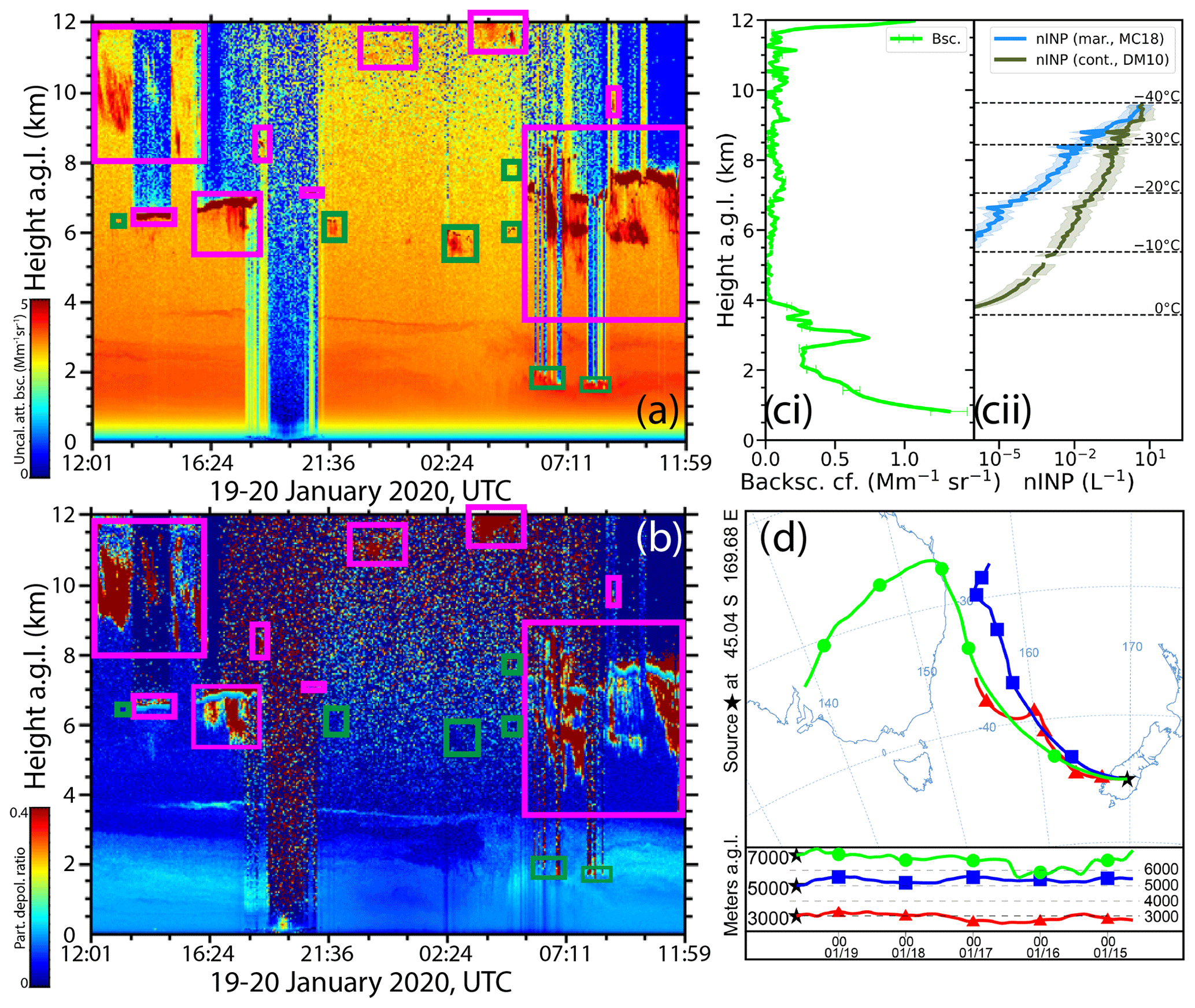
Figure 1Measurement example from Lauder on 19–20 January 2020 corresponding to the Australian cluster 1 from Fig. 9. Temporal development of the uncalibrated attenuated backscatter (a) and particle depolarization ratio (b) at 532 nm wavelength from 19 January 2020, 12:01 UTC, to 20 January 2020, 11:59 UTC, with indicated liquid (green rectangles) and ice-containing clouds (magenta rectangles). Vertical profiles of the particle backscatter coefficient at 532 nm wavelength (20 January 2020, 04:30–04:40 UTC, light green, evaluated with the Klett–Fernald–Sasano algorithm) (ci); INP concentration obtained with conversion parameters from Mamouri and Ansmann (2016) and the parameterizations of McCluskey et al. (2018b, MC18, marine, light blue) and DeMott et al. (2010, DM10, continental, dark green) (cii). The dashed lines indicate the temperatures from GDAS (20 January 2020, 03:00 UTC). Error bars and shaded areas indicate the uncertainty in the retrieved values. HYSPLIT backward trajectories for 120 h arriving at 3, 5, and 7 km height above Lauder at 19 January 2020, 15:00 UTC (d).
3.1 Case study
An example measurement of clouds above Lauder on 19–20 January 2020 UTC is shown in Fig. 1. The temporal developments of the uncalibrated attenuated backscatter coefficient (Fig. 1a) and the particle depolarization ratio (Fig. 1b) at 532 nm show a scene of ice-containing and liquid clouds between roughly 5–9 km height. Up to 3 km height, slightly depolarizing aerosol and at 3.5 km height a lofted aerosol layer were present. Above 9 km height, cirrus clouds were observed. This measurement falls into the period when, above Lauder, elevated smoke layers from the extreme Australian bush fires 2019/20 (Ohneiser et al., 2020; Bègue et al., 2023) were frequently detected. Below 2 km height, some liquid clouds with cloud-top temperatures above 0 ∘C were measured. Furthermore, low clouds/fog impaired the lidar measurements for a short period on 19 January 2020. During this scene, nine ice-containing clouds (indicated with magenta rectangles) and seven liquid clouds (green rectangles, Fig. 1a and b) were classified.
Figure 1c shows vertical profiles of particle backscatter coefficient at 532 nm wavelength (Fig. 1ci) and INP concentration of marine and continental aerosol (Fig. 1cii). The profile was evaluated for a period without lower-level clouds (20 January 2020, 04:30–04:40 UTC). The INP concentration was estimated from the backscatter coefficient using the method and conversion parameters described in Mamouri and Ansmann (2016) and the freezing parameterizations for continental (DeMott et al., 2010) and marine aerosol (McCluskey et al., 2018b), which were applied for the temperature range from −40 to 0 ∘C as in Mamouri and Ansmann (2016). For the liquid cloud on 20 January 2020, 04:43–05:01 UTC, with a cloud top at 7.7 km and a cloud-top temperature at −24 ∘C, this calculation yields INP concentrations at the cloud top of 0.3 L−1 (continental aerosol) and 2 × 10⁻³ L−1 (marine aerosol). For the ice-containing cloud on 20 January 2020, 05:14–12:01 UTC, with a cloud top at 8.9 km and a cloud-top temperature of −34 ∘C, where freezing is occurring probably regardless of the specific aerosol population, this yields INP concentrations at cloud top of 1.5 L−1 (continental) and 0.2 L−1 (marine). In general, the INP concentration estimates for continental (and, respectively, marine) aerosol have the following range: 2 × 10⁻³ L−1 (4 × 10⁻⁷ L−1) at −10 ∘C, 0.06 L−1 (1 × 10⁻⁴ L−1) at −20 ∘C, 0.9 L−1 (0.04 L−1) at −30 ∘C, and 5 L−1 (5 L−1) at −40 ∘C. These differences of up to 4 orders of magnitude emphasize the strong impact that the continental aerosol contribution has on INP concentrations and the potential resulting changes in freezing efficiency. For comparison, Radenz et al. (2021a) reported lidar-derived INP concentrations for Punta Arenas of about 3 × 10⁻⁵ L−1 (7 × 10⁻³ L−1) at −20 ∘C (−30 ∘C) when only pristine marine aerosol is present, while already small quantities (1 %–4 %) of continental aerosol lead to a significant increase of the INP concentrations to about 0.06 L−1 (0.06 L−1) at −20 ∘C (−30 ∘C).
HYSPLIT backward trajectories for 120 h arriving above Lauder at 3, 5, and 7 km height on 19 January 2020, 15:00 UTC, are shown in Fig. 1d. While the lower backward trajectory, probably representative of the near-ground as well as lofted aerosol layer, points towards rather local or regional air mass origin, the upper backward trajectories come from Australia or its direction. Therefore, this measurement example (i.e., the ice-containing cloud on 19 January 2020, 15:59–18:51 UTC, also indicated with one of the magenta rectangles in Fig. 1a and b) belongs to the Australian backward trajectory cluster 1 (Fig. 9a), exhibiting higher ice formation efficiency (Sect. 3.4, Fig. 9b). At lower levels, the air masses were transported slowly due to a weak-gradient high-pressure situation, and only in the upper half of the troposphere (> 6 km height) did a faster flow regime from Australia prevail (NIWA, 2023).
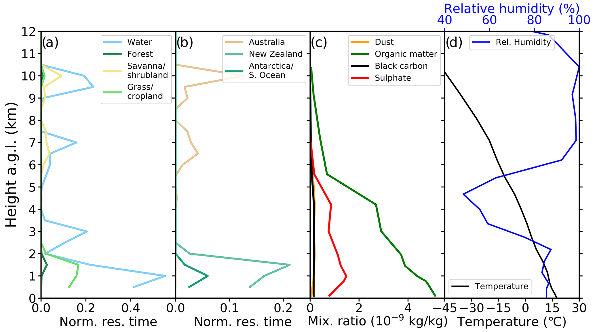
Figure 2Vertical profiles at 19 January 2020, 15:00 UTC, of TRACE normed residence times of surface-cover (a) and named geographical area classifications (b), MACC aerosol mixing ratios excluding sea salt (c), and temperature and relative humidity from GDAS (d).
Figure 2 shows vertical profiles of TRACE surface-cover and named geographical area classifications, MACC aerosol mixing ratios excluding sea salt, and temperature and relative humidity from GDAS temporally closest (19 January 2020, 15:00 UTC) to the abovementioned ice-containing cloud. The TRACE surface-cover classifications indicate air masses influenced by Water and Grass/cropland in the lower altitudes and by Savanna/shrubland (besides Water) in the higher altitudes (Fig. 2a). The TRACE named geographical area classifications (Fig. 2b) indicate air masses influenced by Australia above 5.5 km height and New Zealand and Antarctica/Southern Ocean up to about 2–2.5 km. Although the backward trajectory arriving at 7 km height of the single HYSPLIT run in Fig. 1d is staying exclusively in the free troposphere, the statistical results of TRACE (having a reception height of 2 ) clearly indicate a continental contribution at these heights (Fig. 2a and b). The MACC aerosol mixing ratios (excluding sea salt) are dominated by organic matter and sulfate which are decreasing above 5.5 km, while dust and black carbon are marginal throughout the column (Fig. 2c). According to the GDAS profile, the temperature at 7 km is about −20 ∘C at high relative humidity (Fig. 2d).
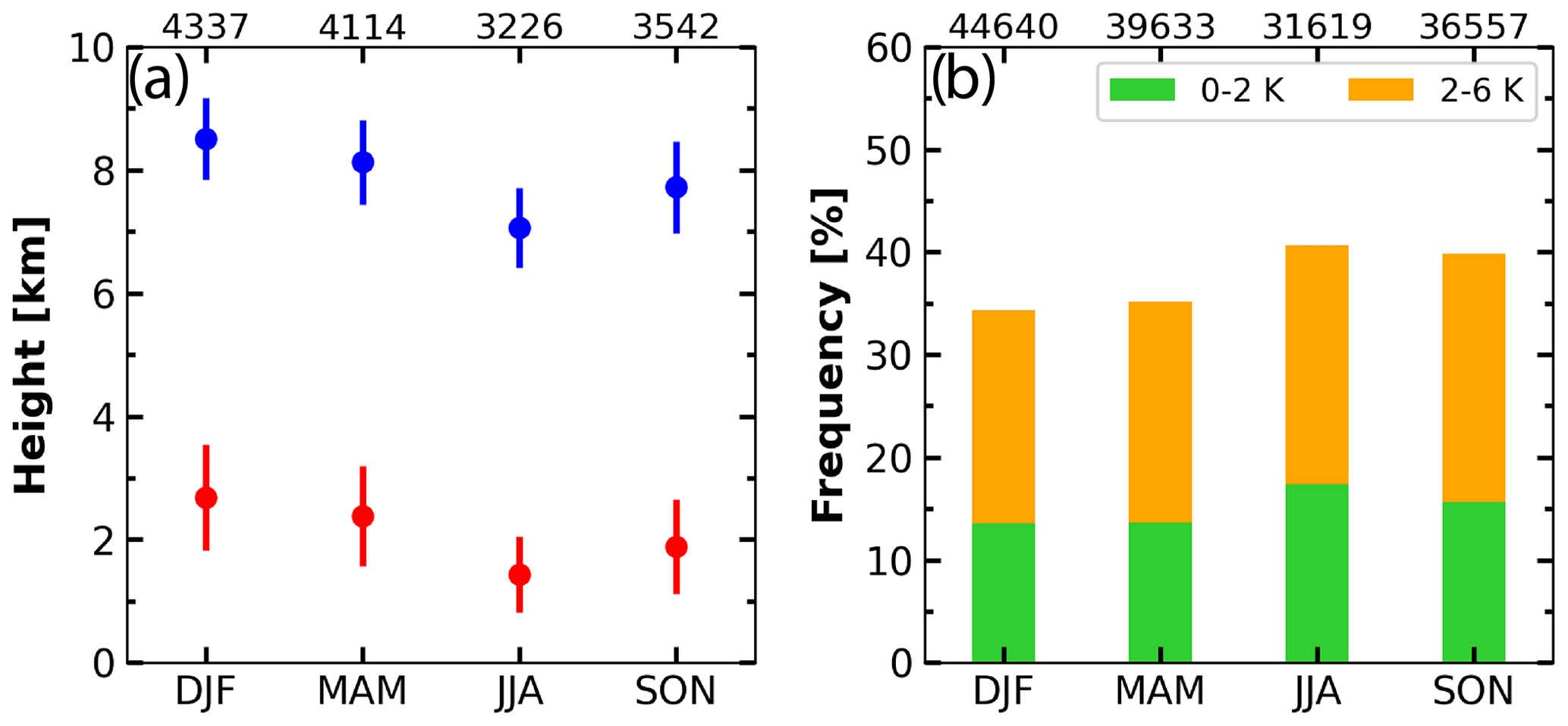
Figure 3Seasonal occurrence of the heterogeneous freezing regime at Invercargill / Waihōpai based on radiosoundings. Panel (a) shows the average heights of the 0 ∘C isotherm (red) and −35 ∘C isotherm (blue). Frequencies of dew point spreads of 0–2 K (green) and 2–6 K (orange) within the heterogeneous freezing temperature range are shown in panel (b). The number of observations are given on the top of each plot. Soundings from 1950–2022 were used.
3.2 Air mass statistics
Before the presentation of the mixed-phase cloud statistics, general information on the conditions for heterogeneous freezing and the aerosol properties are provided in this section. Long-term records of radiosoundings at Invercargill Airport about 200 km southwest of Lauder were used to assess the abundance of thermodynamic conditions under which heterogeneous freezing occurs, namely, temperatures between 0 and −35 ∘C and the availability of moisture. Given the short distance to Lauder, we assume that the conditions are comparable to those from Invercargill / Waihōpai, for which the valuable radiosonde dataset is available. Tradowsky et al. (2018) compared radiosonde and automatic weather station data collected at Lauder and Invercargill / Waihōpai and concluded that especially temperature anomalies are well correlated between these two sites. Figure 3 shows the seasonal occurrence of that heterogeneous freezing regime over Invercargill / Waihōpai. The heights of the isotherms show a maximum in the summer season (austral, DJF) with 2.6 km for the 0 ∘C isotherm and 8.4 km for the −35 ∘C isotherm (Fig. 3a). In austral autumn (MAM), their heights are only slightly lower, while in winter their heights decrease to 7 km for the −35 ∘C isotherm and to 1.4 km for the 0 ∘C isotherm. During spring (SON), the isotherms remain at lower heights than in autumn. Large-scale dew point spreads less than 2 K are usually needed for clouds to form (Poore et al., 1995). Depending on the vertical air motions, dew point spreads up to 6 K could be sufficient as well. Figure 3b shows the relative frequency of dew point spreads between 0–2 K and between 2–6 K, respectively, for heights with temperatures in the heterogeneous freezing regime. The frequencies of the 0–2 K dew point spreads during summer and autumn are nearly equal with 14 %, and the maximum occurs in winter with a frequency of 17 % being only slightly higher than the one in spring. Therefore, suitable conditions for clouds to form in the heterogeneous freezing regime are present throughout the year at Invercargill / Waihōpai. Climatologically, one can assume similar conditions for the site of Lauder, which is just 200 km north of the radiosonde station in Invercargill / Waihōpai. However, due to the vicinity of Lauder to the mountains and associated lee effects, the free troposphere over Lauder might contain less water vapor. Therefore, the average dew point spread might be lower than over Invercargill / Waihōpai. In turn, the likelihood of strong upward motion due to orographic mountain waves might be pronounced over Lauder, which would favor the formation of free-tropospheric cloud layers.
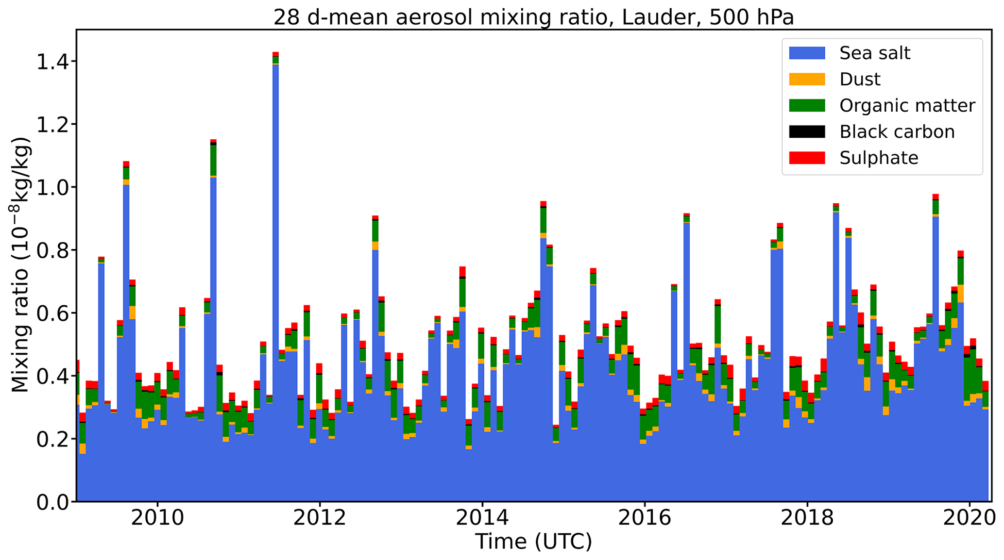
Figure 4Time series of 28 d mean CAMS-MACC sea salt (blue), dust (orange), organic matter (green), black carbon (black), and sulfate (red) aerosol mixing ratios at 500 hPa above Lauder from January 2009 to April 2020.
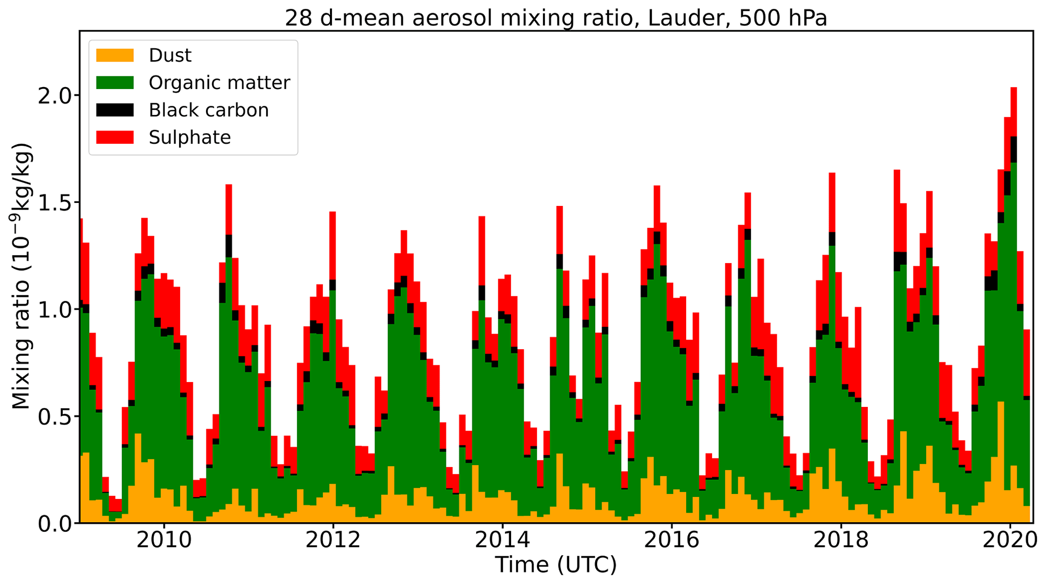
The general aerosol conditions above Lauder were derived based on the MACC dataset. The MACC mixing ratios of the three size ranges of sea salt and dust aerosol species and the species of organic matter and black carbon were summed up and averaged individually on a 28 d time window over the measurement period from January 2009 to April 2020. Figure 4 shows a time series of these 28 d means of the MACC aerosol mixing ratios at the 500 hPa level above Lauder. Obviously, the simulated aerosol mixing ratios are dominated by sea salt which shows weakly pronounced minima during (austral) summer and maxima during (austral) spring. Figure 5 shows the same data at the same pressure level but excluding the dominant sea salt mixing ratio. In strong contrast to the total aerosol mixing ratios, the remaining aerosol mixing ratios show a distinct annual cycle with maxima during (austral) spring or summer. The most abundant species are organic matter followed by dust and sulfate with marginal amounts of black carbon. The simulated aerosol mixing ratios reach exceptionally high values in austral summer 2019/20 due to the Australian bush fires at that time. Based on long-term sun photometer observations, Liley and Forgan (2009) showed that the median aerosol optical thickness (AOT) above Lauder is about 0.03 at 500 nm wavelength with a minimum during austral winter (0.02) and a maximum during austral spring and summer (0.04). They also report no significant variation of AOT with surface humidity below 90 %. The peak in AOT in spring has been attributed to long-range transport of biomass burning products, as implied by the correlation with carbon monoxide measurements presented by Liley et al. (2001) and Jones et al. (2001). With regard to the usage of the MACC mixing ratios (as an indication of aerosol composition and abundance for the analysis of aerosol impact on the formation of mixed-phase clouds), this dominance of sea salt could be obstructive, and, as the annual cycle in Fig. 4 shows, large amounts of sea salt might rather be a tracer of air containing less other aerosol. Therefore, sea salt is omitted in the subsequent analyses and discussions.
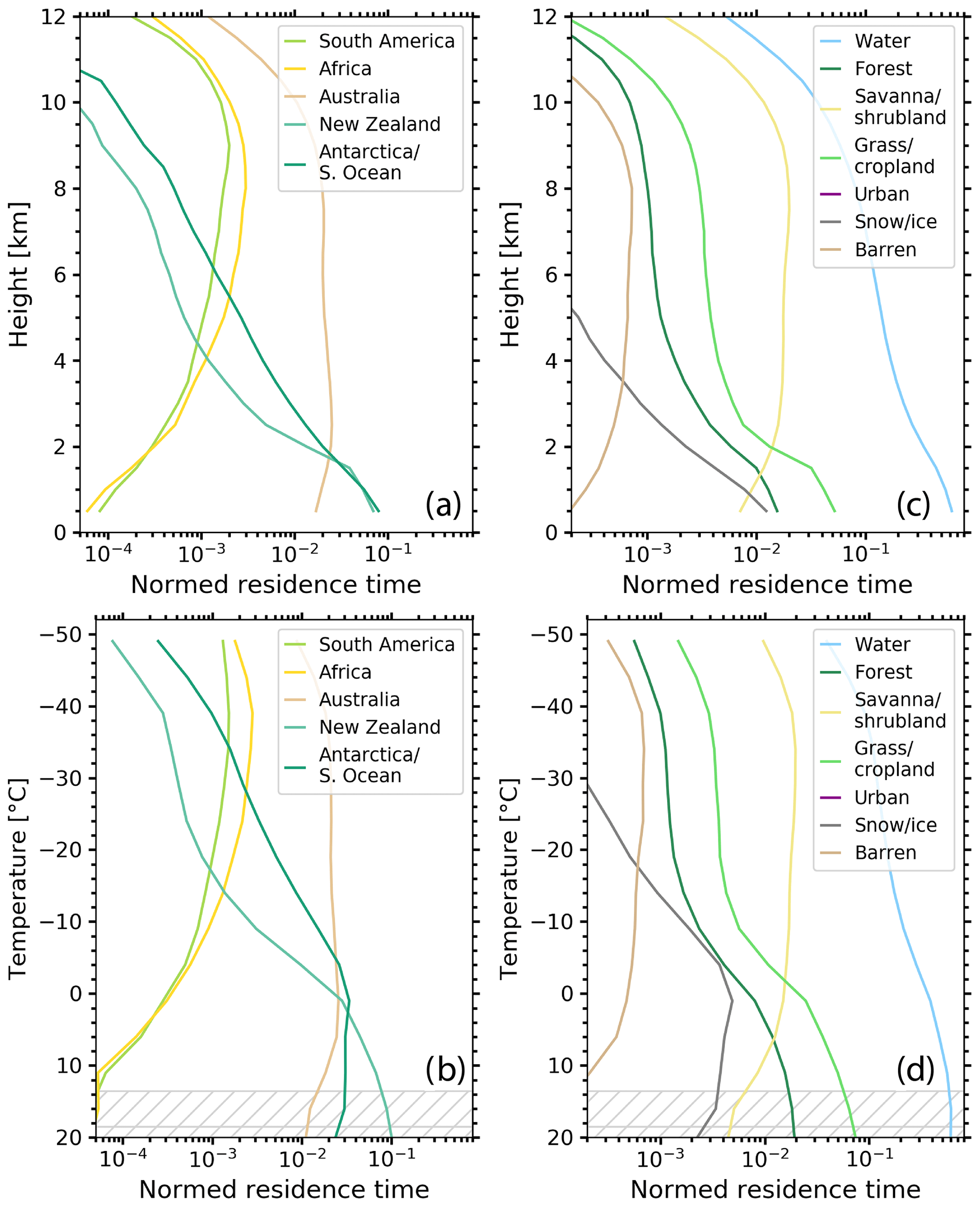
Figure 6Profiles of normed residence times of trajectories above named geographical areas (a, b) and surface-cover classifications (c, d) in terms of kilometers above ground level () (a, c) and temperature (b, d) from the temporally and vertically resolved air mass source attribution tool TRACE (Radenz et al., 2021b).
Results of the temporally and vertically resolved air mass source attribution tool TRACE for trajectories arriving above Lauder are shown in Fig. 6. The height profiles of normed residence times of trajectories above the named geographical areas indicate New Zealand and Antarctica/Southern Ocean as the most important air mass sources up to heights of about 2 km (Fig. 6a). Above that, Australia is the major source of air masses, while Africa and South America show residence times that are an order of magnitude lower. The temperature profiles of named geographical area classifications indicate New Zealand as the major source up to shortly above 0 ∘C, at lower temperatures Antarctica/Southern Ocean and again Australia become more important (Fig. 6b). Regarding the height profiles of normed residence times of trajectories above surface-cover classifications, Water is dominant over the whole column followed by Savanna/shrubland, except in the lowest 1–2 km where the other categories (except Barren) show slightly higher normed residence times (Fig. 6c). In terms of temperature profiles of surface-cover classifications, a very similar picture as in the height profiles is drawn apart from relatively larger residence times above Snow/ice at about −15 to 0 ∘C (Fig. 6d). It can be concluded that Lauder is seeing air masses influenced by New Zealand / Aotearoa and Australia, mainly at heights (temperatures) above (below) 2 km (−5 ∘C), as well as air masses of marine or Southern Ocean origin.
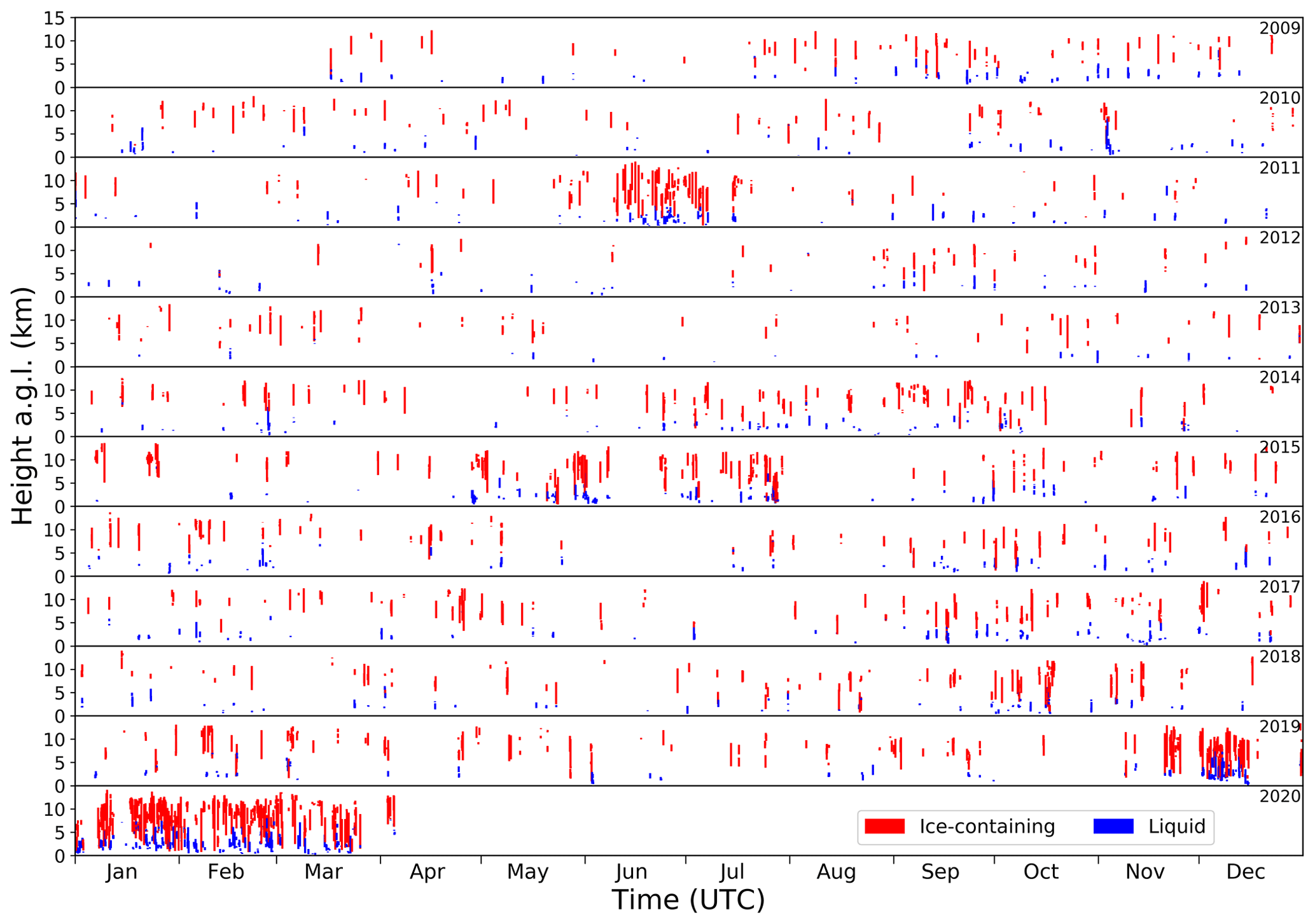
Figure 7Classified liquid (blue) and ice-containing clouds (red) in the height range 0–15 km a.g.l. above Lauder during the analyzed years 2009–2020 (top to bottom).
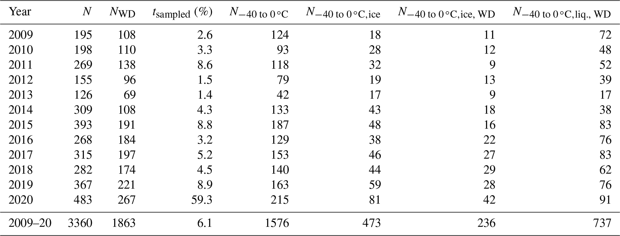
Table 1Overview of the extent of the 11-year Lauder cloud dataset. Number (N) of categorized liquid (liq.) and ice-containing (ice) clouds, including relative time of cloud occurrence (tsampled) for the full dataset and for the subdataset covering the heterogeneous freezing range −40 to 0 ∘C and for clouds with a well-defined (WD) cloud top (see Sect. 2).
3.3 Cloud statistics
In total, the 11-year dataset covers more than 9000 h of polarization lidar measurement data. Figure 7 shows all classified cloud layers from 2009 to 2020. As can be seen from the increased number of classified clouds, three periods in 2011, 2015, and from the end of 2019 until 2020 experienced more frequent lidar observations. These were conducted to characterize the plumes of the erupted Chilean volcanoes Puyehue-Cordón Caulle (2011) and Calbuco (2015) and to obtain a larger database specifically for this study (2019/20). A total of 3360 clouds were identified with a total occurrence time of more than 6000 h, with 1576 out of them in the temperature range between −40 and 0 ∘C. The number of clouds (total, well-defined, in the range of −40 to 0 ∘C, respectively) as well as the relative time covered by the occurrence time of the identified clouds for each year is listed in Table 1. Overall, about 45 % of the observed clouds (1497) did not have a well-defined cloud top due to too large cloud optical thickness. The remaining 1863 clouds were classified as well-defined (WD). In the cloud-top temperature range of −40 to 0 ∘C, 61 % of clouds (973) have a well-defined cloud top. The fraction of ice-containing clouds at a specific cloud-top temperature can be considered characteristic for a certain geographical region and is widely used to describe ice nucleation in models or observations (e.g., Seifert et al., 2015; McCoy et al., 2015; Alexander and Protat, 2018; Villanueva et al., 2021; Radenz et al., 2021a). Figure 8 shows the fraction of ice-containing clouds in eight cloud-top temperature intervals of 5 K from −40 to 0 ∘C for Lauder (this study), Leipzig (Seifert et al., 2010), and Punta Arenas (Kanitz et al., 2011). The error bars denote the statistical uncertainty by the standard error σ defined by the following formula:
with f as the frequency of occurrence of ice-containing clouds and n as the total number of observed clouds in the specific temperature range. The fraction of ice-containing clouds including clouds without well-defined cloud tops is slightly larger at most cloud-top temperature ranges and is shown too (Fig. 8, dashed line). Leipzig (51.4∘ N, 12.4∘ E) represents typical polluted aerosol conditions of the northern midlatitudes (Seifert et al., 2010; Kanitz et al., 2011), while Punta Arenas (53.1∘ S, 70.9∘ W; southern Chile) represents clean and pristine southern midlatitudes (Jimenez et al., 2020; Radenz et al., 2021a). For Lauder, an increase of the relative number of ice-containing clouds is observed at about a temperature range of −20 to −15 ∘C. In this temperature range, the fraction of ice-containing clouds at Lauder is about a factor of 5.4 smaller than at Leipzig and close to that at Punta Arenas. On the other hand, in the temperature range of −30 to −25 ∘C, the fraction of ice-containing clouds at Lauder is 1.3 times smaller than at Leipzig and still 1.6 times larger than at Punta Arenas. Lauder and Punta Arenas are subject to generally low free-tropospheric aerosol loads, which suggests that the lower ice formation efficiency at these two sites compared to Leipzig is related to low INP concentrations.
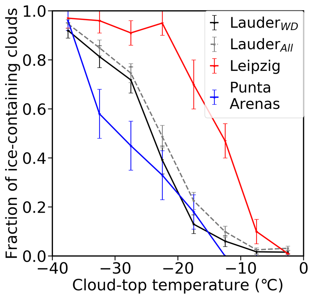
Figure 8Fraction of ice-containing clouds as a function of cloud-top temperature in intervals of 5 K for Leipzig (red; Seifert et al., 2010), Punta Arenas (blue; Kanitz et al., 2011), and Lauder considering only well-defined clouds (black, this study) and all clouds (grey, this study). The error bars represent the statistical significance calculated with Eq. (1).
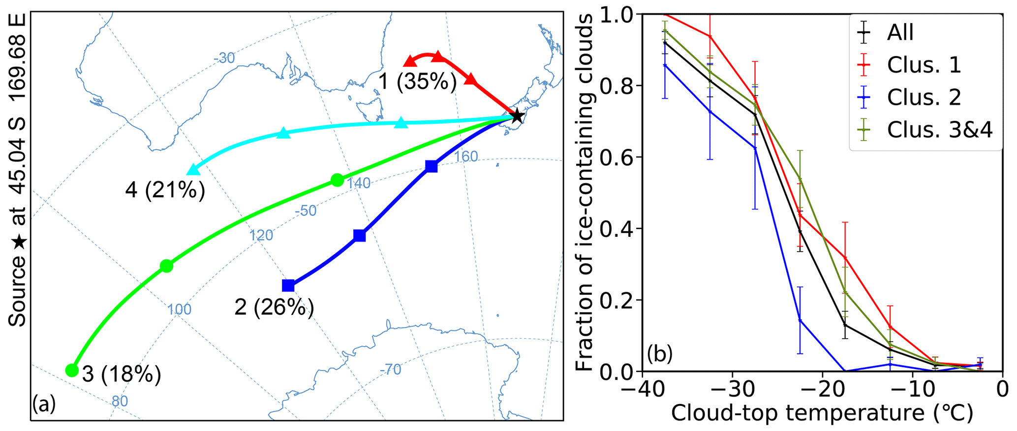
Figure 9Clusters of 1544 (72 h HYSPLIT) backward trajectories arriving at cloud middle height and cloud start time rounded to full hour (the four clusters explain about 85 % of the clustered backward trajectories' total spatial variance) (a); same as Fig. 8 but all well-defined clouds (black, same as in Fig. 8) and well-defined clouds corresponding to cluster 1 (red), cluster 2 (blue), and clusters 3 and 4 (green) (b).
3.4 Separation of clouds based on air mass statistics
Backward trajectory tools were used to investigate the aerosol effect on ice formation efficiency in clouds above Lauder. In a first approach, backward trajectories for each classified well-defined cloud were calculated and clustered (see Sect. 2.3). The resulting clusters are shown in Fig. 9a. Cluster 1 (35 % of trajectories) can be described as direct Australian transport. Contrasting to this, cluster 2 (26 % of trajectories) represents trajectories with fast transport of Antarctic air masses. Clusters 3 (18 %) and 4 (21 % of trajectories) contain trajectories of air masses transported above ocean and, therefore, can be characterized as marine. Figure 9b shows the fraction of ice-containing clouds against cloud-top temperature for all well-defined clouds and for well-defined clouds corresponding to the trajectories in the abovementioned clusters (Fig. 9a). The fast Antarctic transport cluster 2 shows much lower ice formation efficiency. While the Australian cluster 1 shows highest ice formation efficiency, except at the temperature range −25 to −20 ∘C. There, the marine clusters 3 and 4 exhibit larger ice formation efficiencies, albeit within statistical uncertainty.
The MACC model was used to obtain simulated aerosol conditions for each classified well-defined cloud (see Sect. 2.3). The aerosol effect on ice formation efficiency in the observed clouds is investigated by categorizing these clouds based on the simulated aerosol mixing ratios. As discussed in Sect. 3.2, the dominance of sea salt in the simulated aerosol mixing ratios above Lauder might obstruct the assessment of aerosol impact on the formation of mixed-phase clouds. Therefore, two different quantities were defined based on the MACC aerosol mixing ratios to use as a proxy for aerosol abundance. The first one is the MACC total aerosol mixing ratio excluding the sea salt mixing ratio (see the time series in Fig. 5). The second one is the former divided by the sea salt mixing ratio, i.e., the MACC aerosol mixing ratio excluding sea salt relative to sea salt. Varying arbitrary thresholds on these two quantities were then used to categorize the abovementioned clouds. Figure 10 shows the fraction of ice-containing clouds against cloud-top temperature for all well-defined clouds and for well-defined clouds corresponding to increasing MACC total aerosol mixing ratios excluding sea salt as well as increasing MACC aerosol mixing ratios excluding sea salt relative to sea salt. Enhanced ice formation efficiencies were found for clouds experiencing a combination of high aerosol mixing ratios (excluding sea salt) and a low sea salt fraction. This is an indication for higher ice formation efficiency for clouds which are more strongly influenced by continental aerosol.
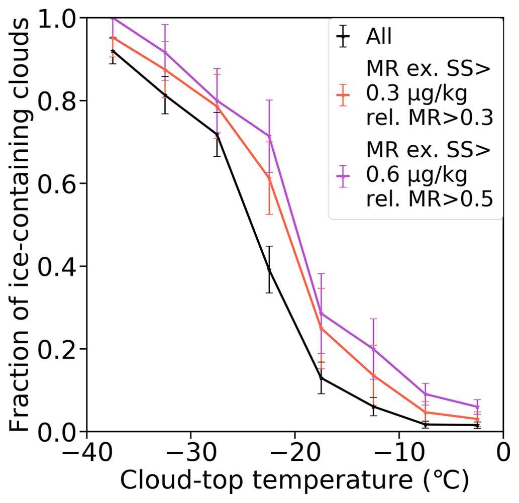
Figure 10Same as Fig. 8 but for all well-defined clouds (black, same as in Fig. 8) and for well-defined clouds corresponding to a combination of criteria, namely, MACC total aerosol mixing ratio excluding sea salt relative to sea salt > 0.3 and MACC total aerosol mixing ratio excluding sea salt > 0.3 µg kg−1 (orange), as well as > 0.5 and > 0.6 µg kg−1, respectively (violet).
This study investigated the impact of variations in the atmospheric aerosol load on the frequency of heterogeneous ice formation over Lauder, New Zealand / Aotearoa. As prerequisites, long-term datasets of polarization lidar observations, atmospheric temperature and humidity profiles from both radiosondes and model reanalyses, and HYSPLIT backward trajectories, as well as of CAMS-MACC aerosol reanalysis data, were acquired and processed. An 11-year polarization lidar dataset from Lauder was analyzed with the Seifert et al. (2010, 2015) methods to assess the ice formation efficiency in clouds with top temperatures in the heterogeneous freezing range from −40 to 0 ∘C. Thereby, the cloud dataset considered only clouds with a lidar-detectable cloud top height, in order to prevent positive temperature biases by deep, attenuating clouds with underestimated cloud tops.
Based on a long-term radiosonde dataset from Invercargill / Waihōpai, New Zealand / Aotearoa, the general conditions for the formation of mixed-phase clouds in the region of southern New Zealand / Aotearoa were characterized. It was found that the −35 ∘C isotherm lies between 7 km (austral winter) and 8.4 km (austral summer). In the heterogeneous freezing temperature range, dew point spreads of 0–2 K occurred with a frequency of 14 % (austral summer) and 17 % (austral winter).
Next, the general aerosol conditions over Lauder were assessed based on a statistical analysis of HYSPLIT back trajectories with the TRACE tool, as well as based on a long-term statistics of CAMS-MACC aerosol reanalyses data. Generally, it was found that sea salt and marine air masses are the dominating aerosol species. Nevertheless, this constant marine background was superimposed by aerosol of considerable variability regarding the air mass source regions and the aerosol load. Both clean, pristine air masses from Antarctica and the Southern Ocean and aerosol-laden air masses from continental Australia occur frequently over New Zealand / Aotearoa. The number of identified cases per air mass was sufficient to split the lidar-based cloud dataset into different subpopulations in order to assess the impact of air mass origin on the frequency of heterogeneous ice formation.
Overall, ice formation efficiency in clouds above Lauder was found to be lower than at Leipzig in the polluted midlatitudes of the Northern Hemisphere but higher than in very clean and pristine environments, such as Punta Arenas in southern Chile, 8000 km downwind of any neighboring landmass. This can be expected as New Zealand / Aotearoa is influenced both by Australian and marine aerosol. Further, the incorporation of the trajectory tools and aerosol model simulations both point clearly to higher ice formation efficiency for clouds which are more strongly influenced by continental aerosol and to lower ice formation efficiency for clouds which are more influenced by Antarctic/marine aerosol and air masses.
In conclusion, it can be stated, based on the outcome of the study, that the atmospheric conditions over the South Island / Te Waipounamu of New Zealand support contrast studies for evaluation of the relationship between aerosol load and mixed-phase cloud formation. We argue that this region is one of the more accessible places in the Southern Hemisphere midlatitudes, where local aerosol sources are scarce while the general circulation permits alternating periods of pristine and aerosol-laden air masses, respectively.
Our study made use of a unique 11-year polarization lidar dataset from Lauder. Other active remote sensing instrumentation was not available for such a long time period over this region. There is, hence, a high potential for future long-term experiments that incorporate additional observational capabilities, specifically of Raman and Doppler lidar as well as cloud Doppler radar. Radenz et al. (2021a) have extensively demonstrated the capabilities of these additional instruments in characterizing (i) the ice-nucleating capabilities of the aerosol mix at cloud level, (ii) the impact of atmospheric gravity waves on the sustained formation of supercooled liquid water, and (iii) the determination of aerosol impacts on ice water mass production as estimated from cloud radar observations. Moreover, cloud radar would allow us to observe the cloud layers in their full extent, which would minimize the number of clouds with undefined cloud top heights/temperatures.
Future studies might also make further use of other atmospheric measurements from the Lauder observatory. Profiles of trace gas concentration could be used as indicators for Southern Ocean and marine air masses. From February 2023, the aerosol lidar at Lauder has been automated for 24 h operation, measuring in alternating 10 min intervals. This will greatly increase the data available for possible extension or refinement of this study.
HYSPLIT backward trajectories are calculated via the available online tools (https://www.ready.noaa.gov/HYSPLIT.php, HYSPLIT, 2023; Stein et al., 2015; Rolph et al., 2017). GDAS data are available at https://www.ready.noaa.gov/gdas1.php (GDAS, 2023). The air mass source attribution tool TRACE is available at https://doi.org/10.5281/zenodo.4438051 (TRACE, 2023; Radenz et al., 2021b). The Invercargill / Waihōpai radiosonde data were obtained through the Integrated Global Radiosonde Archive dataset available at https://www.ncei.noaa.gov/products/weather-balloon/integrated-global-radiosonde-archive (IGRA, 2023; Durre et al., 2006, 2018). The TRACE results, the cloud dataset, the used analysis software, and the lidar data are available on request at TROPOS or NIWA.
JH analyzed the data and drafted the manuscript. JBL conducted the lidar measurements in collaboration with the NIWA Lauder team. OU, IM, TS, and TN made these data available. PS provided data analysis software and transferred the lidar data in a compatible format. MR provided radiosonde data and TRACE air mass source analysis results. PS and AA supervised the work and revised the manuscript. All authors jointly contributed to the paper and the scientific discussion.
The contact author has declared that none of the authors has any competing interests.
Publisher's note: Copernicus Publications remains neutral with regard to jurisdictional claims made in the text, published maps, institutional affiliations, or any other geographical representation in this paper. While Copernicus Publications makes every effort to include appropriate place names, the final responsibility lies with the authors.
We thank Kevin Ohneiser for providing the CAMS-MACC data.
The LOSTECCA (Lidar Observations of SpatioTEmporal Contrasts in Clouds and Aerosols in Lauder, New Zealand / Aotearoa) project is funded by the Federal Ministry of Education and Research of Germany in the context of strategic projects between Germany and New Zealand / Aotearoa under the funding code 01DR20002. This project received support by the European Research Infrastructure for the observations of Aerosol, Clouds, and Trace Gases Research Infrastructure (ACTRIS) under grant agreement nos. 654109 and 739530 from the European Union's Horizon 2020 research and innovation program. Additionally, this project is part of ACTRIS-D, which is funded by the Federal Ministry of Education and Research of Germany under the funding code 01LK2001A. Deep South Challenge and NIWA received funding through the Strategic Science Investment Fund (SSIF) of New Zealand / Aotearoa. The lidar measurements at Lauder are supported in part by the funding of the Greenhouse Gases Observing Satellite (GOSAT) series project.
The publication of this article was funded by the Open Access Fund of the Leibniz Association.
This paper was edited by Markus Petters and reviewed by Alex Schuddeboom and one anonymous referee.
Alexander, S. P. and Protat, A.: Cloud Properties Observed From the Surface and by Satellite at the Northern Edge of the Southern Ocean, J. Geophys. Res.-Atmos., 123, 443–456, https://doi.org/10.1002/2017JD026552, 2018. a, b
Ansmann, A., Tesche, M., Seifert, P., Althausen, D., Engelmann, R., Fruntke, J., Wandinger, U., Mattis, I., and Müller, D.: Evolution of the ice phase in tropical altocumulus: SAMUM lidar observations over Cape Verde, J. Geophys. Res.-Atmos., 114, D17208, https://doi.org/10.1029/2008JD011659, 2009. a, b
Bègue, N., Baron, A., Krysztofiak, G., Berthet, G., Bencherif, H., Kloss, C., Jégou, F., Khaykin, S., Ranaivombola, M., Millet, T., Portafaix, T., Duflot, V., Keckhut, P., Vérèmes, H., Payen, G., Sha, M. K., Coheur, P.-F., Clerbaux, C., Sicard, M., Sakai, T., Querel, R., Liley, B., Smale, D., Morino, I., Ochino, O., Nagai, T., Smale, P., and Robinson, J.: Evidence of a dual African and Australian biomass burning influence on the vertical distribution of aerosol and carbon monoxide over the Southwest Indian Ocean basin in early 2020, EGUsphere [preprint], https://doi.org/10.5194/egusphere-2023-1946, 2023. a
Bodas-Salcedo, A., Williams, K. D., Ringer, M. A., Beau, I., Cole, J. N. S., Dufresne, J.-L., Koshiro, T., Stevens, B., Wang, Z., and Yokohata, T.: Origins of the Solar Radiation Biases over the Southern Ocean in CFMIP2 Models, J. Climate, 27, 41–56, https://doi.org/10.1175/JCLI-D-13-00169.1, 2014. a
Bodas-Salcedo, A., Hill, P. G., Furtado, K., Williams, K. D., Field, P. R., Manners, J. C., Hyder, P., and Kato, S.: Large Contribution of Supercooled Liquid Clouds to the Solar Radiation Budget of the Southern Ocean, J. Climate, 29, 4213–4228, https://doi.org/10.1175/JCLI-D-15-0564.1, 2016. a
Bodas-Salcedo, A., Mulcahy, J. P., Andrews, T., Williams, K. D., Ringer, M. A., Field, P. R., and Elsaesser, G. S.: Strong Dependence of Atmospheric Feedbacks on Mixed-Phase Microphysics and Aerosol-Cloud Interactions in HadGEM3, J. Adv. Model. Earth Sy., 11, 1735–1758, https://doi.org/10.1029/2019MS001688, 2019. a
CAMS: Copernicus Atmosphere Monitoring Service Information, https://atmosphere.copernicus.eu/ (last access: 21 September 2023), 2023. a
Choi, Y.-S., Lindzen, R. S., Ho, C.-H., and Kim, J.: Space observations of cold-cloud phase change, P. Natl. Acad. Sci. USA, 107, 11211–11216, https://doi.org/10.1073/pnas.1006241107, 2010. a
DeMott, P. J., Prenni, A. J., Liu, X., Kreidenweis, S. M., Petters, M. D., Twohy, C. H., Richardson, M. S., Eidhammer, T., and Rogers, D. C.: Predicting global atmospheric ice nuclei distributions and their impacts on climate, P. Natl. Acad. Sci. USA, 107, 11217–11222, https://doi.org/10.1073/pnas.0910818107, 2010. a, b
DeMott, P. J., Prenni, A. J., McMeeking, G. R., Sullivan, R. C., Petters, M. D., Tobo, Y., Niemand, M., Möhler, O., Snider, J. R., Wang, Z., and Kreidenweis, S. M.: Integrating laboratory and field data to quantify the immersion freezing ice nucleation activity of mineral dust particles, Atmos. Chem. Phys., 15, 393–409, https://doi.org/10.5194/acp-15-393-2015, 2015. a
DeMott, P. J., Hill, T. C. J., McCluskey, C. S., Prather, K. A., Collins, D. B., Sullivan, R. C., Ruppel, M. J., Mason, R. H., Irish, V. E., Lee, T., Hwang, C. Y., Rhee, T. S., Snider, J. R., McMeeking, G. R., Dhaniyala, S., Lewis, E. R., Wentzell, J. J. B., Abbatt, J., CLee, C., Sultana, C. M., Ault, A. P., Axson, J. L., Diaz Martinez, M., Venero, I., Santos-Figueroa, G., Stokes, M. D., Deane, G. B., Mayol-Bracero, O. L., Grassian, V. H., Bertram, T. H., Bertram, A. K., Moffett, B. F., and Franc, G. D.: Sea spray aerosol as a unique source of ice nucleating particles, P. Natl. Acad. Sci. USA, 113, 5797–5803, https://doi.org/10.1073/pnas.1514034112, 2016. a
Desai, N., Chandrakar, K. K., Kinney, G., Cantrell, W., and Shaw, R. A.: Aerosol-Mediated Glaciation of Mixed-Phase Clouds: Steady-State Laboratory Measurements, Geophys. Res. Lett., 46, 9154–9162, https://doi.org/10.1029/2019GL083503, 2019. a
Durre, I., Vose, R. S., and Wuertz, D. B.: Overview of the Integrated Global Radiosonde Archive, J. Climate, 19, 53–68, https://doi.org/10.1175/JCLI3594.1, 2006. a
Durre, I., Yin, X., Vose, R. S., Applequist, S., and Arnfield, J.: Enhancing the Data Coverage in the Integrated Global Radiosonde Archive, J. Atmos. Ocean. Tech., 35, 1753–1770, https://doi.org/10.1175/JTECH-D-17-0223.1, 2018. a
Fernald, F. G.: Analysis of atmospheric lidar observations: some comments, Appl. Optics, 23, 652–653, https://doi.org/10.1364/AO.23.000652, 1984. a
Franklin, C. N., Sun, Z., Bi, D., Dix, M., Yan, H., and Bodas-Salcedo, A.: Evaluation of clouds in ACCESS using the satellite simulator package COSP: Global, seasonal, and regional cloud properties, J. Geophys. Res.-Atmos., 118, 732–748, https://doi.org/10.1029/2012JD018469, 2013. a
Gayet, J.-F., Ovarlez, J., Shcherbakov, V., Ström, J., Schumann, U., Minikin, A., Auriol, F., Petzold, A., and Monier, M.: Cirrus cloud microphysical and optical properties at southern and northern midlatitudes during the INCA experiment, J. Geophys. Res.-Atmos., 109, D20206, https://doi.org/10.1029/2004JD004803, 2004. a
GDAS: Global Data Assimilation System, meteorological data base, https://www.ready.noaa.gov/gdas1.php (last access: 21 September 2023), 2023. a, b
Grise, K. M., Polvani, L. M., and Fasullo, J. T.: Reexamining the Relationship between Climate Sensitivity and the Southern Hemisphere Radiation Budget in CMIP Models, J. Climate, 28, 9298–9312, https://doi.org/10.1175/JCLI-D-15-0031.1, 2015. a
Hamilton, D. S., Lee, L. A., Pringle, K. J., Reddington, C. L., Spracklen, D. V., and Carslaw, K. S.: Occurrence of pristine aerosol environments on a polluted planet, P. Natl. Acad. Sci. USA, 111, 18466–18471, https://doi.org/10.1073/pnas.1415440111, 2014. a
Hogan, R. J., Francis, P. N., Flentje, H., Illingworth, A., Quante, M., and Pelon, J.: Characteristics of mixed-phase clouds. I: Lidar, radar and aircraft observations from CLARE'98, Q. J. Roy. Meteor. Soc., 129, 2089–2116, https://doi.org/10.1256/rj.01.208, 2003. a
Hu, Y., Rodier, S., Xu, K., Sun, W., Huang, J., Lin, B., Zhai, P., and Josset, D.: Occurrence, liquid water content, and fraction of supercooled water clouds from combined CALIOP/IIR/MODIS measurements, J. Geophys. Res.-Atmos., 115, D00H34, https://doi.org/10.1029/2009JD012384, 2010. a
Huang, Y., Protat, A., Siems, S. T., and Manton, M. J.: A-Train Observations of Maritime Midlatitude Storm-Track Cloud Systems: Comparing the Southern Ocean against the North Atlantic, J. Climate, 28, 1920–1939, https://doi.org/10.1175/JCLI-D-14-00169.1, 2015. a
Humphries, R. S., Keywood, M. D., Ward, J. P., Harnwell, J., Alexander, S. P., Klekociuk, A. R., Hara, K., McRobert, I. M., Protat, A., Alroe, J., Cravigan, L. T., Miljevic, B., Ristovski, Z. D., Schofield, R., Wilson, S. R., Flynn, C. J., Kulkarni, G. R., Mace, G. G., McFarquhar, G. M., Chambers, S. D., Williams, A. G., and Griffiths, A. D.: Measurement report: Understanding the seasonal cycle of Southern Ocean aerosols, Atmos. Chem. Phys., 23, 3749–3777, https://doi.org/10.5194/acp-23-3749-2023, 2023. a
Hyder, P., Edwards, J. M., Allan, R. P., Hewitt, H. T., Bracegirdle, T. J., Gregory, J. M., Wood, R. A., Meijers, A. J. S., Mulcahy, J., Field, P., Furtado, K., Bodas-Salcedo, A., Williams, K. D., Copsey, D., Josey, S. A., Liu, C., Roberts, C. D., Sanchez, C., Ridley, J., Thorpe, L., Hardiman, S. C., Mayer, M., Berry, D. I., and Belcher, S. E.: Critical Southern Ocean Climate Model Biases Traced to Atmospheric Model Cloud Errors, Nat. Commun., 9, 3625, https://doi.org/10.1038/s41467-018-05634-2, 2018. a
HYSPLIT: HYbrid Single-Particle Lagrangian Integrated Trajectory model, backward trajectory calculation tool, https://www.ready.noaa.gov/HYSPLIT.php (last access: 21 September 2023), 2023. a, b, c
IGRA: Integrated Global Radiosonde Archive, https://www.ncei.noaa.gov/products/weather-balloon/integrated-global-radiosonde-archive (last access: 21 September 2023), 2023. a
Inness, A., Ades, M., Agustí-Panareda, A., Barré, J., Benedictow, A., Blechschmidt, A.-M., Dominguez, J. J., Engelen, R., Eskes, H., Flemming, J., Huijnen, V., Jones, L., Kipling, Z., Massart, S., Parrington, M., Peuch, V.-H., Razinger, M., Remy, S., Schulz, M., and Suttie, M.: The CAMS reanalysis of atmospheric composition, Atmos. Chem. Phys., 19, 3515–3556, https://doi.org/10.5194/acp-19-3515-2019, 2019. a
Jimenez, C., Ansmann, A., Engelmann, R., Donovan, D., Malinka, A., Seifert, P., Wiesen, R., Radenz, M., Yin, Z., Bühl, J., Schmidt, J., Barja, B., and Wandinger, U.: The dual-field-of-view polarization lidar technique: a new concept in monitoring aerosol effects in liquid-water clouds – case studies, Atmos. Chem. Phys., 20, 15265–15284, https://doi.org/10.5194/acp-20-15265-2020, 2020. a, b
Jones, N. B., Rinsland, C. P., Liley, J. B., and Rosen, J.: Correlation of aerosol and carbon monoxide at 45∘ S: Evidence of biomass burning emissions, Geophys. Res. Lett., 28, 709–712, https://doi.org/10.1029/2000GL012203, 2001. a, b
Kajtar, J. B., Santoso, A., Collins, M., Taschetto, A. S., England, M. H., and Frankcombe, L. M.: CMIP5 Intermodel Relationships in the Baseline Southern Ocean Climate System and With Future Projections, Earths Future, 9, e2020EF001873, https://doi.org/10.1029/2020EF001873, 2021. a
Kanitz, T., Seifert, P., Ansmann, A., Engelmann, R., Althausen, D., Casiccia, C., and Rohwer, E. G.: Contrasting the impact of aerosols at northern and southern midlatitudes on heterogeneous ice formation, Geophys. Res. Lett., 38, L17802, https://doi.org/10.1029/2011GL048532, 2011. a, b, c, d, e, f, g
Klett, J. D.: Stable analytical inversion solution for processing lidar returns, Appl. Optics, 20, 211–220, https://doi.org/10.1364/AO.20.000211, 1981. a
Klett, J. D.: Lidar inversion with variable backscatter/extinction ratios, Appl. Optics, 24, 1638–1643, https://doi.org/10.1364/AO.25.000833, 1985. a
Korolev, A., McFarquhar, G., Field, P. R., Franklin, C., Lawson, P., Wang, Z., Williams, E., Abel, S. J., Axisa, D., Borrmann, S., Crosier, J., Fugal, J., Krämer, M., Lohmann, U., Schlenczek, O., Schnaiter, M., and Wendisch, M.: Mixed-Phase Clouds: Progress and Challenges, Meteor. Mon., 58, 5.1–5.50, https://doi.org/10.1175/AMSMONOGRAPHS-D-17-0001.1, 2017. a
Kuma, P., Bender, F. A.-M., Schuddeboom, A., McDonald, A. J., and Seland, Ø.: Machine learning of cloud types in satellite observations and climate models, Atmos. Chem. Phys., 23, 523–549, https://doi.org/10.5194/acp-23-523-2023, 2023. a
Lebo, Z. J., Johnson, N. C., and Harrington, J. Y.: Radiative influences on ice crystal and droplet growth within mixed-phase stratus clouds, J. Geophys. Res.-Atmos., 113, D09203, https://doi.org/10.1029/2007JD009262, 2008. a
Liley, J. B. and Forgan, B. W.: Aerosol optical depth over Lauder, New Zealand, Geophys. Res. Lett., 36, L07811, https://doi.org/10.1029/2008GL037141, 2009. a, b
Liley, J. B., Rosen, J. M., Kjome, N. T., Jones, N. B., and Rinsland, C. P.: Springtime enhancement of upper tropospheric aerosol at 45∘ S, Geophys. Res. Lett., 28, 1495–1498, https://doi.org/10.1029/2000GL012206, 2001. a, b
Lohmann, U. and Feichter, J.: Global indirect aerosol effects: a review, Atmos. Chem. Phys., 5, 715–737, https://doi.org/10.5194/acp-5-715-2005, 2005. a
Mace, G. G., Protat, A., and Benson, S.: Mixed-Phase Clouds Over the Southern Ocean as Observed From Satellite and Surface Based Lidar and Radar, J. Geophys. Res.-Atmos., 126, e2021JD034569, https://doi.org/10.1029/2021JD034569, 2021a. a
Mace, G. G., Protat, A., Humphries, R. S., Alexander, S. P., McRobert, I. M., Ward, J., Selleck, P., Keywood, M., and McFarquhar, G. M.: Southern Ocean Cloud Properties Derived From CAPRICORN and MARCUS Data, J. Geophys. Res.-Atmos., 126, e2020JD033368, https://doi.org/10.1029/2020JD033368, 2021b. a
Mallet, M. D., Humphries, R. S., Fiddes, S. L., Alexander, S. P., Altieri, K., Angot, H., Anilkumar, N., Bartels-Rausch, T., Creamean, J., Dall'Osto, M., Dommergue, A., Frey, M., Henning, S., Lannuzel, D., Lapere, R., Mace, G. G., Mahajan, A. S., McFarquhar, G. M., Meiners, K. M., Miljevic, B., Peeken, I., Protat, A., Schmale, J., Steiner, N., Sellegri, K., Simó, R., Thomas, J. L., Willis, M. D., Winton, V. H. L., and Woodhouse, M. T.: Untangling the influence of Antarctic and Southern Ocean life on clouds, Elementa, 11, 00130, https://doi.org/10.1525/elementa.2022.00130, 2023. a
Mamouri, R.-E. and Ansmann, A.: Potential of polarization lidar to provide profiles of CCN- and INP-relevant aerosol parameters, Atmos. Chem. Phys., 16, 5905–5931, https://doi.org/10.5194/acp-16-5905-2016, 2016. a, b, c
McCluskey, C. S., Hill, T. C. J., Humphries, R. S., Rauker, A. M., Moreau, S., Strutton, P. G., Chambers, S. D., Williams, A. G., McRobert, I., Ward, J., Keywood, M. D., Harnwell, J., Ponsonby, W., Loh, Z. M., Krummel, P. B., Protat, A., Kreidenweis, S. M., and DeMott, P. J.: Observations of Ice Nucleating Particles Over Southern Ocean Waters, Geophys. Res. Lett., 45, 11989–11997, https://doi.org/10.1029/2018GL079981, 2018a. a
McCluskey, C. S., Ovadnevaite, J., Rinaldi, M., Atkinson, J., Belosi, F., Ceburnis, D., Marullo, S., Hill, T. C. J., Lohmann, U., Kanji, Z. A., O'Dowd, C., Kreidenweis, S. M., and DeMott, P. J.: Marine and Terrestrial Organic Ice-Nucleating Particles in Pristine Marine to Continentally Influenced Northeast Atlantic Air Masses, J. Geophys. Res.-Atmos., 123, 6196–6212, https://doi.org/10.1029/2017JD028033, 2018b. a, b
McCluskey, C. S., DeMott, P. J., Ma, P.-L., and Burrows, S. M.: Numerical Representations of Marine Ice-Nucleating Particles in Remote Marine Environments Evaluated Against Observations, Geophys. Res. Lett., 46, 7838–7847, https://doi.org/10.1029/2018GL081861, 2019. a
McCoy, D. T., Hartmann, D. L., Zelinka, M. D., Ceppi, P., and Grosvenor, D. P.: Mixed-phase cloud physics and Southern Ocean cloud feedback in climate models, J. Geophys. Res.-Atmos., 120, 9539–9554, https://doi.org/10.1002/2015JD023603, 2015. a
McFarquhar, G. M., Bretherton, C. S., Marchand, R., Protat, A., DeMott, P. J., Alexander, S. P., Roberts, G. C., Twohy, C. H., Toohey, D., Siems, S., Huang, Y., Wood, R., Rauber, R. M., Lasher-Trapp, S., Jensen, J., Stith, J., Mace, J., Um, J., Järvinen, E., Schnaiter, M., Gettelman, A., Sanchez, K. J., McCluskey, C. S., Russell, L. M., McCoy, I. L., Atlas, R. L., Bardeen, C. G., Moore, K. A., Hill, T. C. J., Humphries, R. S., Keywood, M. D., Ristovski, Z., Cravigan, L., Schofield, R., Fairall, C., Mallet, M. D., Kreidenweis, S. M., Rainwater, B., D'Alessandro, J., Wang, Y., Wu, W., Saliba, G., Levin, E. J. T., Ding, S., Lang, F., Truong, S. C. H., Wolff, C., Haggerty, J., Harvey, M. J., Klekociuk, A. R., and McDonald, A.: Observations of Clouds, Aerosols, Precipitation, and Surface Radiation over the Southern Ocean: An Overview of CAPRICORN, MARCUS, MICRE, and SOCRATES, B. Am. Meteorol. Soc., 102, E894–E928, https://doi.org/10.1175/BAMS-D-20-0132.1, 2021. a
Minikin, A., Petzold, A., Ström, J., Krejci, R., Seifert, M., van Velthoven, P., Schlager, H., and Schumann, U.: Aircraft observations of the upper tropospheric fine particle aerosol in the Northern and Southern Hemispheres at midlatitudes, Geophys. Res. Lett., 30, 1503, https://doi.org/10.1029/2002GL016458, 2003. a
Morcrette, J.-J., Boucher, O., Jones, L., Salmond, D., Bechtold, P., Beljaars, A., Benedetti, A., Bonet, A., Kaiser, J. W., Razinger, M., Schulz, M., Serrar, S., Simmons, A. J., Sofiev, M., Suttie, M., Tompkins, A. M., and Untch, A.: Aerosol analysis and forecast in the European Centre for Medium-Range Weather Forecasts Integrated Forecast System: Forward modeling, J. Geophys. Res.-Atmos., 114, D06206, https://doi.org/10.1029/2008JD011235, 2009. a
Nagai, T., Liley, B., Sakai, T., Shibata, T., and Uchino, O.: Post-Pinatubo Evolution and Subsequent Trend of the Stratospheric Aerosol Layer Observed by Mid-Latitude Lidars in Both Hemispheres, SOLA, 6, 69–72, https://doi.org/10.2151/sola.2010-018, 2010. a
Nakamae, K., Uchino, O., Morino, I., Liley, B., Sakai, T., Nagai, T., and Yokota, T.: Lidar observation of the 2011 Puyehue-Cordón Caulle volcanic aerosols at Lauder, New Zealand, Atmos. Chem. Phys., 14, 12099–12108, https://doi.org/10.5194/acp-14-12099-2014, 2014. a
NIWA: NIWA National Climate Centre: New Zealand Climate Summary, January 2020, https://niwa.co.nz/sites/niwa.co.nz/files/Climate_Summary_January_2020-NIWA.pdf (last access: 21 September 2023), 2023. a
Ohneiser, K., Ansmann, A., Baars, H., Seifert, P., Barja, B., Jimenez, C., Radenz, M., Teisseire, A., Floutsi, A., Haarig, M., Foth, A., Chudnovsky, A., Engelmann, R., Zamorano, F., Bühl, J., and Wandinger, U.: Smoke of extreme Australian bushfires observed in the stratosphere over Punta Arenas, Chile, in January 2020: optical thickness, lidar ratios, and depolarization ratios at 355 and 532 nm, Atmos. Chem. Phys., 20, 8003–8015, https://doi.org/10.5194/acp-20-8003-2020, 2020. a
Platt, C. M. R.: Lidar Backscatter from Horizontal Ice Crystal Plates, J. Appl. Meteorol. Clim., 17, 482–488, https://doi.org/10.1175/1520-0450(1978)017<0482:LBFHIC>2.0.CO;2, 1978. a
Poore, K. D., Wang, J., and Rossow, W. B.: Cloud layer thicknesses from a combination of surface and upper-air observations, J. Climate, 8, 550–568, https://doi.org/10.1175/1520-0442(1995)008<0550:CLTFAC>2.0.CO;2, 1995. a
Possner, A., Ekman, A. M. L., and Lohmann, U.: Cloud response and feedback processes in stratiform mixed-phase clouds perturbed by ship exhaust, Geophys. Res. Lett., 44, 1964–1972, https://doi.org/10.1002/2016GL071358, 2017. a
Radenz, M., Bühl, J., Seifert, P., Baars, H., Engelmann, R., Barja González, B., Mamouri, R.-E., Zamorano, F., and Ansmann, A.: Hemispheric contrasts in ice formation in stratiform mixed-phase clouds: disentangling the role of aerosol and dynamics with ground-based remote sensing, Atmos. Chem. Phys., 21, 17969–17994, https://doi.org/10.5194/acp-21-17969-2021, 2021a. a, b, c, d, e, f, g, h
Radenz, M., Seifert, P., Baars, H., Floutsi, A. A., Yin, Z., and Bühl, J.: Automated time–height-resolved air mass source attribution for profiling remote sensing applications, Atmos. Chem. Phys., 21, 3015–3033, https://doi.org/10.5194/acp-21-3015-2021, 2021b. a, b, c, d
Rauber, R. M. and Tokay, A.: An Explanation for the Existence of Supercooled Water at the Top of Cold Clouds, J. Atmos. Sci., 48, 1005–1023, https://doi.org/10.1175/1520-0469(1991)048<1005:AEFTEO>2.0.CO;2, 1991. a
Rolph, G., Stein, A., and Stunder, B.: Real-time Environmental Applications and Display sYstem: READY, Environ. Modell. Softw., 95, 210–228, https://doi.org/10.1016/j.envsoft.2017.06.025, 2017. a, b
Sakai, T., Uchino, O., Nagai, T., Liley, B., Morino, I., and Fujimoto, T.: Long-term variation of stratospheric aerosols observed with lidars over Tsukuba, Japan, from 1982 and Lauder, New Zealand, from 1992 to 2015, J. Geophys. Res.-Atmos., 121, 10283–10293, https://doi.org/10.1002/2016JD025132, 2016. a
Sasano, Y., Browell, E. V., and Ismail, S.: Error caused by using a constant extinction/backscattering ratio in the lidar solution, Appl. Optics, 24, 3929–3932, https://doi.org/10.1364/AO.24.003929, 1985. a
Schuddeboom, A. J. and McDonald, A. J.: The Southern Ocean Radiative Bias, Cloud Compensating Errors, and Equilibrium Climate Sensitivity in CMIP6 Models, J. Geophys. Res.-Atmos., 126, e2021JD035310, https://doi.org/10.1029/2021JD035310, 2021. a
Seifert, A., Köhler, C., and Beheng, K. D.: Aerosol-cloud-precipitation effects over Germany as simulated by a convective-scale numerical weather prediction model, Atmos. Chem. Phys., 12, 709–725, https://doi.org/10.5194/acp-12-709-2012, 2012. a
Seifert, P., Ansmann, A., Mattis, I., Wandinger, U., Tesche, M., Engelmann, R., Müller, D., Pérez, C., and Haustein, K.: Saharan dust and heterogeneous ice formation: Eleven years of cloud observations at a central European EARLINET site, J. Geophys. Res.-Atmos., 115, D20201, https://doi.org/10.1029/2009JD013222, 2010. a, b, c, d, e, f, g
Seifert, P., Ansmann, A., Groß, S., Freudenthaler, V., Heinold, B., Hiebsch, A., Mattis, I., Schmidt, J., Schnell, F., Tesche, M., Wandinger, U., and Wiegner, M.: Ice formation in ash-influenced clouds after the eruption of the Eyjafjallajökull volcano in April 2010, J. Geophys. Res.-Atmos., 116, D00U04, https://doi.org/10.1029/2011JD015702, 2011. a
Seifert, P., Kunz, C., Baars, H., Ansmann, A., Bühl, J., Senf, F., Engelmann, R., Althausen, D., and Artaxo, P.: Seasonal variability of heterogeneous ice formation in stratiform clouds over the Amazon Basin, Geophys. Res. Lett., 42, 5587–5593, https://doi.org/10.1002/2015GL064068, 2015. a, b, c
Shupe, M. D. and Intrieri, J. M.: Cloud Radiative Forcing of the Arctic Surface: The Influence of Cloud Properties, Surface Albedo, and Solar Zenith Angle, J. Climate, 17, 616–628, https://doi.org/10.1175/1520-0442(2004)017<0616:CRFOTA>2.0.CO;2, 2004. a
Solomon, A., de Boer, G., Creamean, J. M., McComiskey, A., Shupe, M. D., Maahn, M., and Cox, C.: The relative impact of cloud condensation nuclei and ice nucleating particle concentrations on phase partitioning in Arctic mixed-phase stratocumulus clouds, Atmos. Chem. Phys., 18, 17047–17059, https://doi.org/10.5194/acp-18-17047-2018, 2018. a
Stein, A. F., Draxler, R. R., Rolph, G. D., Stunder, B. J. B., Cohen, M. D., and Ngan, F.: NOAA's HYSPLIT atmospheric transport and dispersion modeling system, B. Am. Meteorol. Soc., 96, 2059–2077, https://doi.org/10.1175/BAMS-D-14-00110.1, 2015. a, b
Stephens, G. L.: Cloud Feedbacks in the Climate System: A Critical Review, J. Climate, 18, 237–273, https://doi.org/10.1175/JCLI-3243.1, 2005. a
Sun, Z. and Shine, K. P.: Studies of the radiative properties of ice and mixed-phase clouds, Q. J. Roy. Meteor. Soc., 120, 111–137, https://doi.org/10.1002/qj.49712051508, 1994. a
Tan, I., Storelvmo, T., and Choi, Y.-S.: Spaceborne lidar observations of the ice-nucleating potential of dust, polluted dust, and smoke aerosols in mixed-phase clouds, J. Geophys. Res.-Atmos., 119, 6653–6665, https://doi.org/10.1002/2013JD021333, 2014. a
Tatzelt, C., Henning, S., Welti, A., Baccarini, A., Hartmann, M., Gysel-Beer, M., van Pinxteren, M., Modini, R. L., Schmale, J., and Stratmann, F.: Circum-Antarctic abundance and properties of CCN and INPs, Atmos. Chem. Phys., 22, 9721–9745, https://doi.org/10.5194/acp-22-9721-2022, 2022. a, b
Tegen, I., Hollrig, P., Chin, M., Fung, I., Jacob, D., and Penner, J.: Contribution of different aerosol species to the global aerosol extinction optical thickness: Estimates from model results, J. Geophys. Res.-Atmos., 102, 23895–23915, https://doi.org/10.1029/97JD01864, 1997. a
TRACE: Software for automated trajectory analysis, Zenodo [software], https://doi.org/10.5281/zenodo.4438051, 2023. a, b
Tradowsky, J. S., Bodeker, G. E., Querel, R. R., Builtjes, P. J. H., and Fischer, J.: Combining data from the distributed GRUAN site Lauder–Invercargill, New Zealand, to provide a site atmospheric state best estimate of temperature, Earth Syst. Sci. Data, 10, 2195–2211, https://doi.org/10.5194/essd-10-2195-2018, 2018. a
Trenberth, K. E. and Fasullo, J. T.: Simulation of Present-Day and Twenty-First-Century Energy Budgets of the Southern Oceans, J. Climate, 23, 440–454, https://doi.org/10.1175/2009JCLI3152.1, 2010. a, b
Uchino, O., Tabata, I., Kai, K., and Okada, Y.: Polarization Properties of Middle and High Level Clouds Observed by Lidar, J. Meteorol. Soc. Jpn., 66, 607–616, https://doi.org/10.2151/jmsj1965.66.4_607, 1988. a
Uchino, O., Nagai, T., Fujimoto, T., Matthews, W. A., and Orange, J.: Extensive lidar observations of the Pinatubo aerosol layers at Tsukuba (36.1∘ N), Naha (26.2∘ N), Japan and Lauder (45.0∘ S), New Zealand, Geophys. Res. Lett., 22, 57–60, https://doi.org/10.1029/94GL02735, 1995. a
U.S. Government Printing Office: U.S. Standard Atmosphere, 1976, U.S. Government Printing Office, Washington, DC, 1976. a
Varma, V., Morgenstern, O., Field, P., Furtado, K., Williams, J., and Hyder, P.: Improving the Southern Ocean cloud albedo biases in a general circulation model, Atmos. Chem. Phys., 20, 7741–7751, https://doi.org/10.5194/acp-20-7741-2020, 2020. a
Vergara-Temprado, J., Murray, B. J., Wilson, T. W., O'Sullivan, D., Browse, J., Pringle, K. J., Ardon-Dryer, K., Bertram, A. K., Burrows, S. M., Ceburnis, D., DeMott, P. J., Mason, R. H., O'Dowd, C. D., Rinaldi, M., and Carslaw, K. S.: Contribution of feldspar and marine organic aerosols to global ice nucleating particle concentrations, Atmos. Chem. Phys., 17, 3637–3658, https://doi.org/10.5194/acp-17-3637-2017, 2017. a
Villanueva, D., Heinold, B., Seifert, P., Deneke, H., Radenz, M., and Tegen, I.: The day-to-day co-variability between mineral dust and cloud glaciation: a proxy for heterogeneous freezing, Atmos. Chem. Phys., 20, 2177–2199, https://doi.org/10.5194/acp-20-2177-2020, 2020. a
Villanueva, D., Neubauer, D., Gasparini, B., Ickes, L., and Tegen, I.: Constraining the Impact of Dust-Driven Droplet Freezing on Climate Using Cloud-Top-Phase Observations, Geophys. Res. Lett., 48, e2021GL092687, https://doi.org/10.1029/2021GL092687, 2021. a
Welti, A., Bigg, E. K., DeMott, P. J., Gong, X., Hartmann, M., Harvey, M., Henning, S., Herenz, P., Hill, T. C. J., Hornblow, B., Leck, C., Löffler, M., McCluskey, C. S., Rauker, A. M., Schmale, J., Tatzelt, C., van Pinxteren, M., and Stratmann, F.: Ship-based measurements of ice nuclei concentrations over the Arctic, Atlantic, Pacific and Southern oceans, Atmos. Chem. Phys., 20, 15191–15206, https://doi.org/10.5194/acp-20-15191-2020, 2020. a
Westbrook, C. D., Illingworth, A. J., O'Connor, E. J., and Hogan, R. J.: Doppler lidar measurements of oriented planar ice crystals falling from supercooled and glaciated layer clouds, Q. J. Roy. Meteor. Soc., 136, 260–276, https://doi.org/10.1002/qj.528, 2010. a
Wilson, T. W., Ladino, L. A., Alpert, P. A., Breckels, M. N., Brooks, I. M., Browse, J., Burrows, S. M., Carslaw, K. S., Huffman, J. A., Judd, C., Kilthau, W. P., Mason, R. H., McFiggans, G., Miller, L. A., Nájera, J. J., Polishchuk, E., Rae, S., Schiller, C. L., Si, M., Vergara-Temprado, J., Whale, T. F., Wong, J. P. S., Wurl, O., Yakobi-Hancock, J. D., Abbatt, J. P. D., Aller, J. Y., Bertram, A. K., Knopf, D., and Murray, B. J.: A marine biogenic source of atmospheric ice nucleating particles, Nature, 525, 234–238, https://doi.org/10.1038/nature14986, 2015. a
Zelinka, M. D., Myers, T. A., McCoy, D. T., Po-Chedley, S., Caldwell, P. M., Ceppi, P., Klein, S. A., and Taylor, K. E.: Causes of Higher Climate Sensitivity in CMIP6 Models, Geophys. Res. Lett., 47, e2019GL085782, https://doi.org/10.1029/2019GL085782, 2020. a
Zhang, D., Wang, Z., Kollias, P., Vogelmann, A. M., Yang, K., and Luo, T.: Ice particle production in mid-level stratiform mixed-phase clouds observed with collocated A-Train measurements, Atmos. Chem. Phys., 18, 4317–4327, https://doi.org/10.5194/acp-18-4317-2018, 2018. a
Zhao, X., Liu, X., Burrows, S. M., and Shi, Y.: Effects of marine organic aerosols as sources of immersion-mode ice-nucleating particles on high-latitude mixed-phase clouds, Atmos. Chem. Phys., 21, 2305–2327, https://doi.org/10.5194/acp-21-2305-2021, 2021. a
Zuidema, P., Baker, B., Han, Y., Intrieri, J., Key, J., Lawson, P., Matrosov, S., Shupe, M., Stone, R., and Uttal, T.: An Arctic Springtime Mixed-Phase Cloudy Boundary Layer Observed during SHEBA, J. Atmos. Sci., 62, 160–176, https://doi.org/10.1175/JAS-3368.1, 2005. a