Impact of methane and other precursor emission reductions on surface ozone in Europe: scenario analysis using the European Monitoring and Evaluation Programme (EMEP) Meteorological Synthesizing Centre – West (MSC-W) model

The impacts of future methane (CH₄) and other precursor emission changes are investigated for surface ozone (O₃) in the United Nations Economic Commission for Europe (UNECE) region excluding North America and Israel (the EMEP region, for European Monitoring and Evaluation Programme) for the year 2050. The analysis includes a current legislation (CLE) and maximum feasible technical reduction (MFR) scenario, as well as a scenario that combines MFRs with an additional dietary shift that also meets the Paris Agreement objectives with respect to greenhouse gas emissions (LOW). For each scenario, background CH₄ concentrations are calculated using a probabilistic Earth system model emulator and combined with other precursor emissions in a three-dimensional Eulerian chemistry-transport model. While focus is placed on peak season maximum daily 8 h average (MDA8) O₃ concentrations, a range of other indicators for health and vegetation impacts are also discussed. Our analysis shows that roughly one-third of the total peak season MDA8 reduction achieved between the 2050 CLE and MFR scenarios is attributable to CH₄ reductions, resulting predominantly from CH₄ emission reductions outside of the EMEP region. The impact of other precursor emission reductions is split nearly evenly between the reductions inside and outside of the EMEP region. However, the relative importance of CH₄ and other precursor emission reductions is shown to depend on the choice of O₃ indicator, though indicators sensitive to peak O₃ show generally consistent results. The analysis also highlights the synergistic impacts of CH₄ mitigation as reducing solely CH₄ achieves, beyond air quality improvement, nearly two-thirds of the total global warming reduction calculated for the LOW scenario compared to the CLE case.

1 Introduction

Surface ozone (O₃) is an important source of air pollution, impacting both human and ecosystem health (Lefohn et al., 2018; Monks et al., 2015). In the lower troposphere, the majority of O₃ is produced by the photochemical reaction of nitrogen oxides (NO_x = NO+NO₂) in volatile organic compound (VOC)-rich environments (Crutzen et al., 1999). The most abundant VOC precursor species is methane (CH₄), having a present-day volume mixing ratio of around 1915 ppb (parts per billion) (Lan et al., 2024). Moreover, CH₄ mixing ratios are likely to increase further, as anthropogenic CH₄ emissions are anticipated to increase in the coming decade (UNEP, 2021; Saunois et al., 2020; Höglund-Isaksson et al., 2020). In addition to being a source of air pollution, CH₄ is also the second most important anthropogenic greenhouse gas (GHG), with its importance as both an air pollutant and a global warming agent having received considerable attention in recent years (Mar et al., 2022; Abernethy et al., 2021; Fiore et al., 2008; Dentener et al., 2005).

In this study, the impact of CH₄ and other precursor emissions is investigated for the European Monitoring and Evaluation Programme (EMEP) region, which includes the member countries of the United Nations Economic Commission for Europe (UNECE) region excluding North America and Israel. Focus is placed on the population-weighted exposure to peak season (April–September) average maximum daily 8 h mean (MDA8) O₃ concentrations, being the health indicator employed by the new World Health Organization (WHO) guidelines (WHO, 2021). The latter recommends a peak season MDA8 exposure limit of 60 µg m⁻³ based on the association between long-term O₃ exposure and all-cause mortality, with an interim target of 70 µg m⁻³ for areas where initial exposure is high. To our knowledge, neither the guideline nor interim target values are met in any of the countries within the EMEP region at present. In addition to being employed by the WHO, the focus on peak season MDA8 is also motivated by the broader association between the exposure to peak O₃ and all-cause mortality (Huangfu and Atkinson, 2020).

The impacts on O₃ are investigated for a current legislation (CLE), maximum feasible technical reduction (MFR), and MFR with an additional dietary shift and Paris Agreement policy scenario (LOW) up to the year 2050. The CLE scenario includes the currently agreed upon policies for the abatement of air pollutant and GHG emissions, while the MFR scenario combines the economic activity pathway of the CLE scenario with the full implementation of the best available emission reduction technologies defined in the GAINS (Greenhouse Gas and Air Pollution Interactions and Synergies) model (Amann et al., 2011). The LOW scenario extends the MFR by including climate policies compatible with the Paris Agreement objectives and an additional shift in agricultural practices, bringing further CH₄ and other precursor emission reductions. Relative to the year 2015, global anthropogenic CH₄ emissions decline by 35 % and 50 % in the LOW scenario by 2030 and 2050, respectively, making the reductions comparable to those of the Global Methane Pledge (30 % by 2030, Malley et al., 2023) and Global Methane Assessment (45 % abatement target for 2050, UNEP, 2021).

The emission scenarios are combined with the Model for the Assessment of Greenhouse Gas Induced Climate Change v7.5.3 (MAGICC7) (Meinshausen et al., 2020, 2011, 2009) to calculate their respective background CH₄ concentrations up to the year 2050. To calculate the impacts on surface O₃, the CH₄ projections are specified in the three-dimensional Eulerian chemistry-transport model (CTM) developed at the EMEP Meteorological Synthesizing Centre – West (hereafter EMEP model), where they are also combined with the other precursor scenario emissions. The EMEP model has a long history of policy support and research development (e.g., Jonson et al., 2018; Simpson, 2013; Simpson et al., 2012), with one of its main tasks being the modeling of transboundary fluxes of air pollutants as part of the UNECE Convention on Long-Range Transboundary Air Pollution (CLRTAP) (EMEP MSC-W et al., 2023). In this capacity, the EMEP model has previously been used in support of the review of the UNECE Gothenburg Protocol (Protocol to Abate Acidification, Eutrophication and Ground-level Ozone). The current work in part aims to contribute to the discussion surrounding the second revision of the Gothenburg Protocol, for which the impact of CH₄ on surface O₃ plays a prominent role.

The emission scenarios and their implementation are described in more detail Sect. 2. The MAGICC7 model is described in Sect. 3, where it is also used to calculate background CH₄ concentrations up to the year 2050. Section 4 describes the EMEP model configuration, while also evaluating the baseline configuration against 5 years of observations across Europe. For the scenario calculations presented in Sect. 5, the default modeling configuration involves averaging all results over 5 meteorological years, while a linear latitudinal CH₄ gradient is imposed to capture the effects of inter-hemispheric variations in emissions. Section 5 further combines regional EMEP model simulations with global simulations to quantify the separate impacts of emission changes inside and outside of the EMEP region. While focus is placed on the peak season MDA8 indicator, scenario results for a range of other O₃ health and vegetation indicators are also presented. The results are discussed and compared against earlier studies in Sect. 6, followed by a conclusion in Sect. 7.

2 Emissions

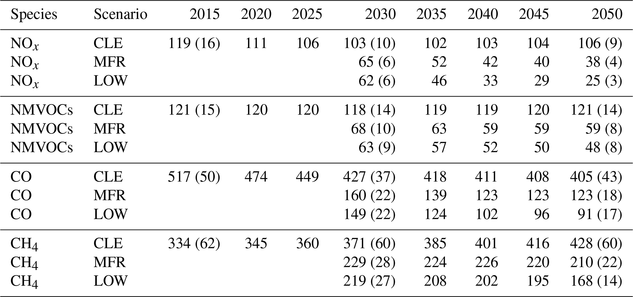
The emission scenarios were developed using the global version of the GAINS model (Winiwarter et al., 2018; Klimont et al., 2017; Amann et al., 2011; Höglund-Isaksson, 2012) and provided by the EMEP Centre for Integrated Assessment Modelling (CIAM) hosted by the Institute for Applied Systems Analysis (IIASA). The scenarios include annual anthropogenic emission totals of CH₄, NO_x, non-methane volatile organic compounds (NMVOCs), carbon monoxide (CO), sulfur oxides (SO_x), ammonia (NH₃), primary fine particulate matter (PM_2.5), and primary coarse PM (PM_co), as well as the carbonaceous fraction of primary PM represented by black carbon (BC) and organic carbon (OC). In the context of the current work, the key emission species are CH₄, NO_x, CO, and NMVOCs, where the latter three affect the lifetime of CH₄ by acting as either net sources (NO_x) or sinks (CO and NMVOCs) of hydroxyl (OH). OH in turn affects the lifetime of CH₄ by loss against oxidation. The global emission totals for the key species are shown in Table 1, along with their respective emissions within the EMEP region for the years 2015, 2030, and 2050.

The emission scenarios span the period from the baseline year 2015 up to 2050 in 5-year intervals, with the MFR and LOW scenarios diverging from the CLE scenario from 2025 onwards. The latter is motivated by the political process of agreeing upon and enforcing effective implementation of the proposed emission control strategies taking at least a few years. Year 2026 being the first year where annual emission totals differ can therefore be considered an optimistic target. In the EMEP model, natural emissions of soil NO_x are included based on monthly climatological values from the CAMS-GLOB-SOIL v2.4 inventory (Simpson and Darras, 2021), noting that soil NO_x emissions from the application of manures and mineral nitrogen fertilizers on agricultural land are calculated in the GAINS model. Forest fire emissions are included based on the daily Fire INventory from NCAR version 2.5 (FINNv2.5, Wiedinmyer et al., 2023) dataset, derived from fire detections from the Moderate Resolution Imaging Spectroradiometer (MODIS) and Visible Infrared Imaging Radiometer Suite (VIIRS) satellite instruments. Forest fire emissions are kept fixed to that of the simulation's meteorological year, also for the future scenario calculations.

Table 1 Global emission totals for the CLE, MFR, and LOW emission scenarios in units of Tg yr⁻¹. Emission totals within the EMEP region, as defined in Sect. 1, are listed in brackets for the years 2015, 2030, and 2050. NO_x emissions have a molecular weight of 46 g mol⁻¹.

2.1 Emission scenarios

2.1.1 CLE scenario

The CLE scenario assumes the implementation and effective enforcement of all currently committed energy and environmental policies affecting emissions of air pollutants and greenhouse gases. CIAM has undertaken a review and update of historical data (up to 2020) driving emissions of all species in the GAINS model, drawing on information from the statistical office of the European Union (EUROSTAT), International Energy Agency (IEA), and UN Food and Agriculture Organization (FAO), in addition to data and emissions reported to the Centre on Emission Inventories and Projections (CEIP). For the EU27 countries, the energy and agriculture projections are consistent with the objectives of the European Green Deal and Fit for 55 package to make the EU carbon neutral by 2050, while also being consistent with the projections used in the EU Third Clean Air Outlook (https://environment.ec.europa.eu/topics/air/clean-air-outlook_en, last access: April 2024). For the western Balkan, Republic of Moldova, Georgia, and Ukraine, a similar set of modeling tools was used as for the EU, developing a new consistent set of projections. For other world regions, the GAINS model downscales projections from IEA and FAO (Alexandratos and Bruinsma, 2012; IEA, 2018), considering updated air pollution legislation from national and international sources (e.g., He et al., 2021; Zhang, 2018), including EU legislation and their implementation in consultation with the EU member states. For the CLE scenario, the socio-economic activity assumptions are similar to that of the Shared Socioeconomic Pathway 2 with an end-of-century radiative forcing of 4.5 W m⁻² (SSP2-4.5). The SSP2-4.5 scenario describes the middle of the road for future societal development, as described in Meinshausen et al. (2020), O’Neill et al. (2017), and Riahi et al. (2017) for a range of SSP scenarios. For the background CH₄ calculations described in Sect. 3, the CLE scenario emissions are therefore combined with GHG emissions (e.g., CO₂ and hydrofluorocarbons) from the SSP2-4.5 scenario. We note that the CLE scenario used in this work does not include the impact of recent shock events (e.g., COVID-19).

2.1.2 MFR mitigation scenario

The MFR mitigation scenario assumes the full implementation of the proven technical mitigation potential as included in the GAINS model for precursor emissions (Amann et al., 2020, 2013; Rafaj et al., 2018) and CH₄ (Gomez Sanabria et al., 2022). Technologies to abate air pollution precursor emissions include, for example, end-of-pipe technologies applied in the power, industry, and transport sector; technology change in industry and residential combustion; and measures in agriculture addressing emissions from manures and mineral fertilizer application by, for example, improved manure management techniques and the construction of low-emission housing including covered manure stores. The fossil fuel and solvent sector emissions include improved flaring, maintenance, leakage, and distribution control measures, as well as low-solvent product substitutions. Global emissions of NO_x, NMVOCs, and CO decline by nearly 80 % by 2050 relative to the 2015 baseline, while CH₄ emissions fall by 37 %. These reductions are driven by the rapid introduction of stringent emission limit values for stationary and mobile sources, strong decline in fossil fuel use, and access to clean energy for cooking. The MFR energy and agricultural activity projections are the same as those of the CLE scenario, with the MFR scenario also being combined with GHG emissions from the SSP2-4.5 scenario.

2.1.3 LOW mitigation scenario

The LOW mitigation scenario extends the MFR by including several additional policies targeting significant transformations in the agricultural sector. This transformation leads to strong reductions in livestock numbers, especially cattle and pigs. The scenario is based in part on the 2019 Growing Better report (The Food and Land Use Coalition, 2019) and other studies addressing healthy dietary requirements (Kanter et al., 2020; Willett et al., 2019), as used in earlier scenarios for global air pollution studies (Amann et al., 2020). While the LOW scenario has the same energy projections as the CLE for EU27 countries, the rest of the world now includes climate policies compatible with Paris Agreement goals, making the GHG emissions consistent with those of the “taking the green road” SSP1-2.6 scenario (Riahi et al., 2017; O’Neill et al., 2017). In the LOW scenario, global CH₄ emission decline by 34 % and 50 % relative to the 2015 baseline by 2030 and 2050, respectively.

2.2 Model implementation

The annual mean national and sector (e.g., road traffic and agriculture) emission totals are distributed in time using a set of monthly, weekly, daily, and hourly time factors based on the global and European CAMS-TEMPO datasets described in Guevara et al. (2021, 2020a, b). For the regional EMEP modeling domain discussed in Sect. 4, the native 0.5°×0.5° scenario emissions are redistributed to the 0.1°×0.1° spatial distribution of the most recent EMEP reported emissions (2021) for countries within the EMEP region (EMEP/CEIP, 2023). However, following the approach used for the first Gothenburg Protocol review, native 0.1°×0.1° gridded emissions from CIAM are used for countries located within the western Balkan and Economic Co-operation and Development, Eastern Europe, Caucasus and Central Asia (EECCA) regions, as well as for Türkiye. Countries that lie (partially) within the regional modeling domain but that are not part of the EMEP region, such as North African countries, follow the global 0.5°×0.5° gridded emissions. International shipping emissions also follow the global 0.5°×0.5° spatial distribution provided by CIAM for all simulations. We further note that direct emissions of CH₄ are not included in the EMEP model, with concentrations instead being specified on an annual mean basis, as discussed in Sect. 4.

3 Background CH₄

Earth system emulators, sometimes known as reduced complexity models (RCMs), have a long history of development as low-cost alternatives to full-complexity climate models. RCMs include simplified parameterizations of, for example, ocean heat uptake, GHG effective radiative forcing, and climate feedbacks, to efficiently estimate future change in climate variables such as GHG concentrations and global mean surface air temperature (GSAT) (Nicholls et al., 2021, 2020). To this end, the MAGICC7 v7.5.3 RCM has been used in the Intergovernmental Panel on Climate Change (IPCC) Sixth Assessment Report (AR6) (Forster et al., 2021), calibrated to capture the relationship between emissions and GSAT for the AR6 historical temperature assessment (Nicholls et al., 2022). In the current work, the MAGGIC7 model is run using the 5-yearly annual emission totals from Table 1, linearly interpolated to annual values and combined with their respective SSP GHG scenario emissions.

In the MAGICC7 model, CH₄ sinks are represented by loss against OH in the troposphere, loss to the stratosphere, and soil uptake (Meinshausen et al., 2011). Climate sensitivities for these mechanisms arise from, for example, temperature-driven changes in atmospheric composition, changes in the Brewer–Dobson circulation strength, and changes in soil properties. CH₄ sources are controlled by the separate contributions arising from anthropogenic, natural, and permafrost emissions. Permafrost is assumed to start thawing when global mean temperatures rise 1° K above pre-industrial levels, with the permafrost module incorporating effects such as polar amplification, soil-specific thawing and decomposition rates, and soil water uptake (Schneider von Deimling et al., 2012). Natural emissions are estimated by closing the CH₄ budget between the years 2015–2023, for which the IIASA emissions are the same for all scenarios, using observed global mean background CH₄ concentrations up to the most recent year for reference (1923 ppb by 2023, Lan et al., 2024). With this approach, natural emissions are estimated at 214.9 Tg yr⁻¹, falling within the top-down range of 194–267 Tg yr⁻¹ reported by Saunois et al. (2020) for the year 2017. The natural emissions are kept constant throughout the simulation period.

A key feature of the MAGICC7 model is that it can be run in a probabilistic mode, where the results of its 600-member ensemble reflect the uncertainties in the parameters controlling future climate change (Nicholls et al., 2022). However, the initial parameter values controlling the CH₄ cycle are the same for each ensemble run, with parameters such as the initial lifetime of CH₄ (9.95 yr⁻¹) and temperature sensitivity of the loss against OH (0.07 K⁻¹) calibrated to match the projections by Holmes et al. (2013) across the range of Representative Concentration Pathway (RCP) scenarios (Meinshausen et al., 2020). As a result, the inter-ensemble variations for the calculated CH₄ projections represent the sensitivity of the different CH₄ source and sink terms to temperature change. We note that the net land-to-atmosphere CH₄ flux from permafrost is found to make a relatively small contribution to the ensemble simulation results, with its 600-ensemble mean emissions falling below 4 Tg yr⁻¹ by 2050 for all scenarios. Nevertheless, its 5-95 % range amounts to 0.5–11.2 Tg yr⁻¹ in the 2050 CLE scenario, compared to a 0.1–2.3 Tg yr⁻¹ range in 2015. Thus illustrating that permafrost emissions can increase by 9 Tg yr⁻¹ for some ensemble members, representing a 4 %–5 % increase in total natural emissions.

CH₄ projections

Figure 1 shows the CH₄ projections calculated for the CLE, MFR, and LOW scenarios, with the shaded regions indicating the 5th to 95th percentile (5 %–95 %) range of the 600-ensemble model output. Here the CH₄ projections for the SSP1-2.6, SSP2-4.5, and SSP5-8.5 scenarios are also included for reference, noting that the IIASA scenario projections fall within the range of the optimistic (SSP1-2.6) and pessimistic (SSP5-8.5) scenarios. While the SSP3-7.0 scenario is the most pessimistic in terms of CH₄ emissions (Meinshausen et al., 2020), its calculated CH₄ concentrations only begin to diverge from the SSP5-8.5 scenario roughly from 2060 onward, and it is therefore not discussed here. For the CLE, MFR, and LOW scenarios, the 2050 global mean CH₄ concentrations and their 5 %–95 % range are calculated as 2236 [2166–2299], 1651 [1597–1700], and 1574 [1512–1627] ppb, respectively. For other years, ensemble mean CH₄ concentrations are shown in Supplement Table S1.

Figure 1 shows that the (temperature-driven) MFR and LOW scenario uncertainties partly overlap. However, the inter-scenario difference between the CLE and the MFR (and LOW) scenarios far exceeds the temperature-driven uncertainties, with the 2050 ensemble mean difference amounting to 585 ppb. In the current work, the difference between the 2050 CLE and the MFR scenarios represents an important measure of the impact of CH₄ emission changes, as this represents the largest inter-scenario concentration difference. While both scenarios have a 5 %–95 % range of approximately 100 ppb by 2050, the 5 %–95 % interval of the difference between the 2050 CLE and MFR scenarios amounts to 571–598 ppb. Thus illustrating that ensemble members with a comparatively high CH₄ concentration in the CLE scenario also have a comparatively high concentration in the MFR scenario and that the ensemble mean scenario difference of 585 ppb is therefore robust.

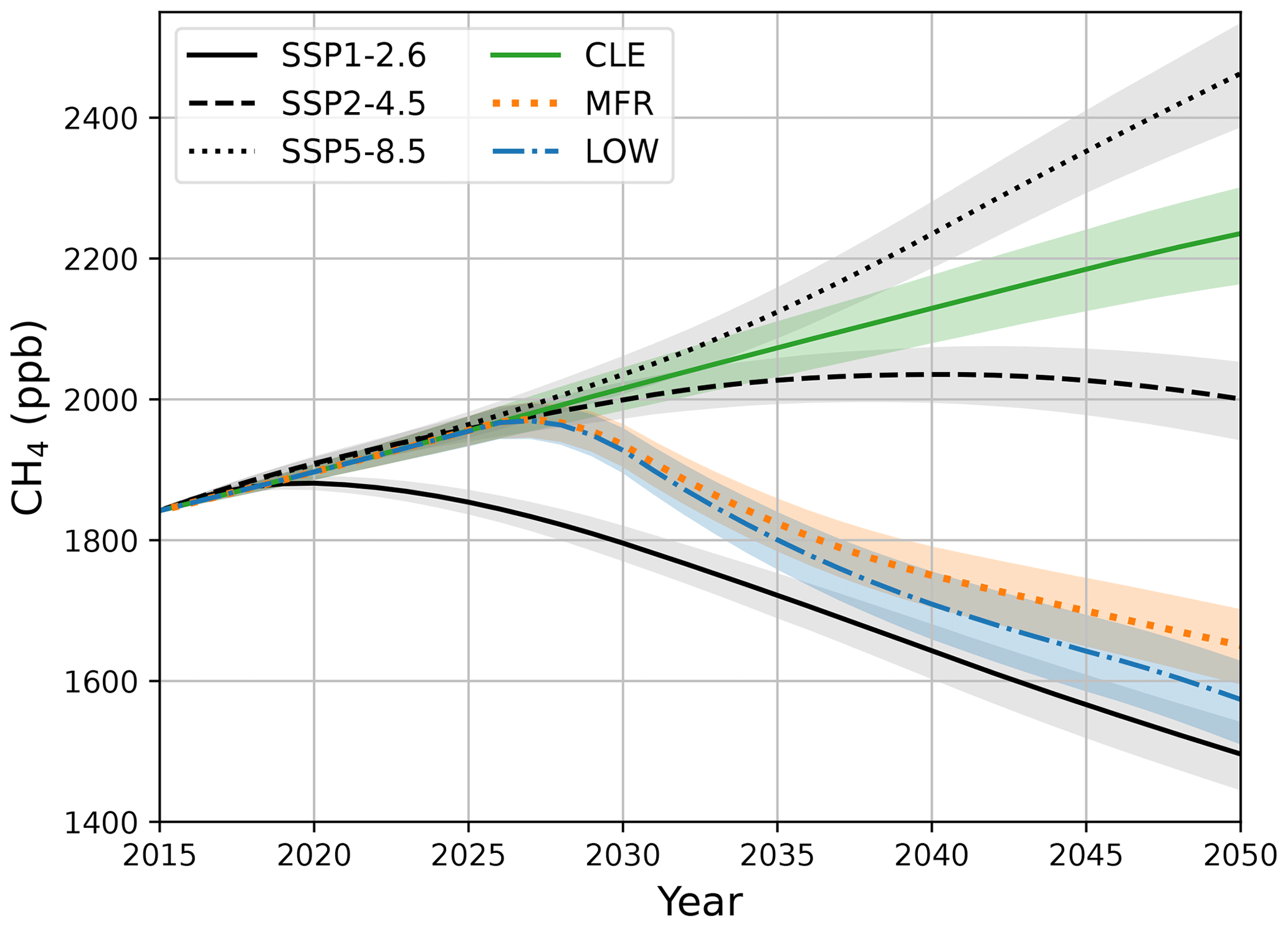
Figure 1 Projected background CH₄ concentrations up to 2050 for the CLE, MFR, and LOW scenarios described in the text. Projections for the SSP5-8.5, SSP2-4.5, and SSP1-2.6 scenarios are included for reference. Shaded areas represent the 600-ensemble 5 %–95 % range.

Diagnostic simulations for a scenario where CH₄ emissions follow the LOW scenario while all other emissions follow those of the CLE scenario (LOW-CH₄) are also performed. This hypothetical scenario thereby reflects a situation where CH₄ emissions are reduced strongly, while no further abatement policies are implemented for the other emissions. In reality, however, CH₄ reductions likely also lead to a reduction in other co-emitted species. The resulting 2050 LOW-CH₄ concentration of 1440 [1392–1484] ppb is comparable to that of the LOW scenario, although lower by 134 ppb (−8.5 %) due to the higher emissions of other lifetime-affecting precursor species. The LOW-CH₄ scenario thereby illustrates that the difference in CH₄ concentrations between the 2050 CLE and LOW scenarios (and corollary MFR) is primarily driven by the difference in the direct emissions of CH₄ and to a lesser extent by the difference in other precursor emissions. A diagnostic LOW scenario where the other GHGs are based on SSP2-4.5 rather than SSP1-2.6 finds that the GHGs from the SSP1-2.6 scenario have very little impact on the simulated CH₄ concentrations (<4 ppb difference by 2050 for all ensemble members). We further note that continuing the CH₄ projections into 2055 with the emissions fixed to that of 2050 leads to an additional change in the ensemble mean concentrations of 38 ppb (1.7 %), −45 ppb (−2.7 %), and −70 ppb (−4.45 %) for the CLE, MFR, and LOW scenarios, respectively. The latter illustrates that, as expected, the CH₄ source and sink terms have not yet reached equilibrium by 2050, owing to the relatively long lifetime of CH₄.

4 EMEP model description

The current work uses EMEP model version rv5.3, as described in more detail by EMEP MSC-W (2023) (for Meteorological Synthesizing Centre – West) and others (e.g., Ge et al., 2024; van Caspel et al., 2023; Stadtler et al., 2018; Simpson et al., 2012). The model employs 20 vertical hybrid pressure–σ levels for the regional 0.1°×0.1° EMEP modeling domain (30–82° N, 30° W–90° E) and 19 vertical levels for the global 0.5°×0.5° modeling domain. The regional and global grids use 3 h meteorological data derived from the ECMWF Integrated Forecasting System (IFS) cycle 40r1 model (ECMWF, 2014). The EMEP model uses its default EmChem19 mechanism (Bergström et al., 2022), designed to balance computational complexity with realism by employing a simplified set of lumped VOC species (Ge et al., 2024). In EmChem19, NO_x is emitted with a 95:5 ratio for NO₂ : NO over land areas. Over pristine maritime environments, half the NO_x emissions are instead placed in a ShipNO_x pseudo-species and chemically converted to HNO₃ to capture the effects of ship plume chemistry (Simpson et al., 2015). While the EMEP model and its chemistry are fully time dependent, background CH₄ and H₂ concentrations are specified at the start of each run and kept fixed throughout the simulation period. However, the chemistry involved with the latter species (e.g., loss of OH and the subsequent chain of reactions leading to O₃ formation from the oxidation of CH₄) remains fully interactive. Hydrogen gas (H₂) is specified with a fixed global concentration of 500 ppb.

In the EMEP model, 3 h IFS O₃ concentrations are specified at the model top (100 hPa) boundary condition, while output surface concentrations are adjusted to an equivalent altitude of 3 m. For the lateral boundary conditions (LBCs) in the regional simulations, 6 h output fields from global simulations are used, with each of the global simulations employing a spin-up period of 6 months. Diagnostic simulations find that the choice of LBC time resolution has a negligibly small impact on the simulation results, while choosing 6 h over 3 h LBCs saves considerable computation time. Output fields from the global model are also used as initial conditions for the regional runs. The geographical region spanned by the regional EMEP modeling domain contains the EMEP region but also parts of North Africa and Asia, whose emissions are consistently treated as the rest of the world (ROW) between the global and regional simulations. For reference, the EMEP region as represented in the regional EMEP modeling domain is shown in Supplement Fig. S1.

4.1 CH₄ implementation

As discussed above, global mean CH₄ concentrations are specified at the start of each run and remain unchanged over the course of the simulation. However, observed CH₄ concentrations display a marked latitudinal gradient, primarily due to the presence of large natural and anthropogenic emission sources in the Northern Hemisphere. The latitudinal gradient can be described by its two leading empirical orthogonal functions (EOFs), or principal components (Meinshausen et al., 2017). The first EOF (EOF1) represents a nearly linear north–south gradient, while the second EOF (EOF2) represents a local northern mid-latitude maximum of ∼10 ppb. EOF1 has a pre-industrial north-to-south-pole gradient of around 40–50 ppb and of around 90 ppb for the year 2014 (Meinshausen et al., 2017). To capture the main characteristics of the latitudinal gradient, the contribution of EOF1 is included in the EMEP model by specifying

$$\begin{array}{}\text{(1)}& {\mathrm{CH}}_{\mathrm{4}}(\mathit{\varphi },{{\mathrm{CH}}_{\mathrm{4}}}^{*})={{\mathrm{CH}}_{\mathrm{4}}}^{*}\left(\mathrm{1}+{\displaystyle \frac{\mathrm{0.025}\mathit{\varphi }}{\mathrm{90}}}\right),\end{array}$$

where ${{\mathrm{CH}}_{\mathrm{4}}}^{*}$ represents the global mean background concentration and ϕ is latitude in degrees. For pre-industrial (808 ppb) and year 2015 (1834 ppb) global mean CH₄ concentrations, Eq. (1) yields latitudinal gradients of 40 and 92 ppb, respectively, consistent with those described in Meinshausen et al. (2017). By applying Eq. (1) also for the projected CH₄ concentrations, an approach similar to that of Meinshausen et al. (2020) is followed, by effectively using EOF1 to extrapolate the latitudinal gradient into the future based on anthropogenic CH₄ emissions.

4.2 Scenario configurations

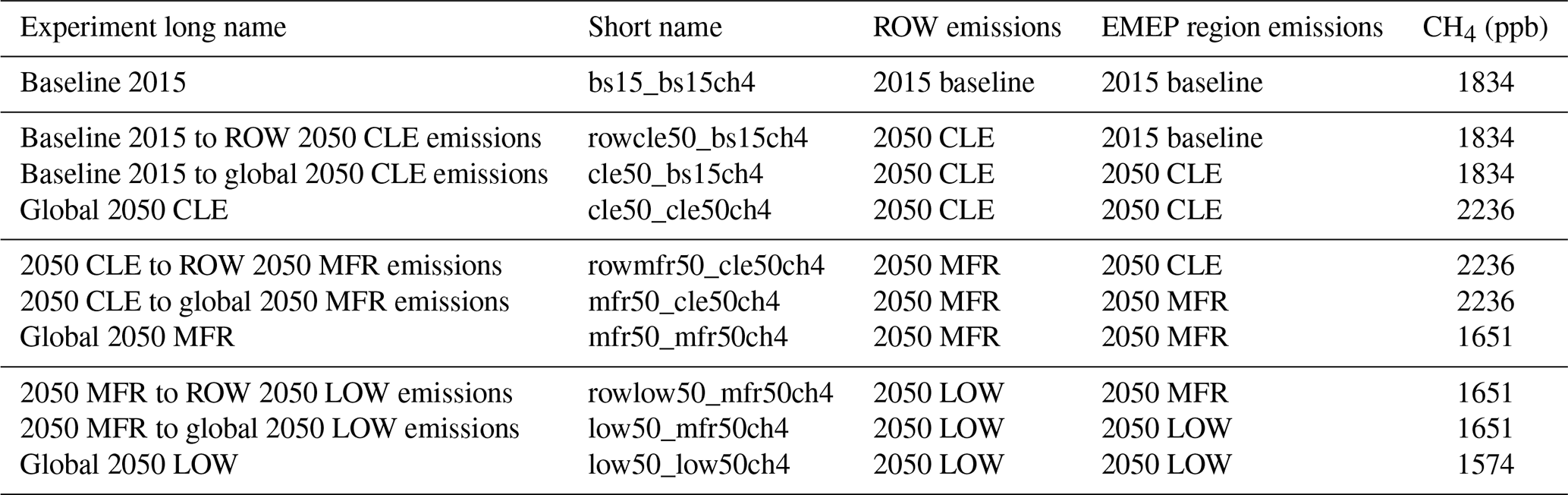
To simulate the effects of precursor emission changes inside and outside of the EMEP region, regional simulations are combined with LBCs from the global model configuration. Simulations where only background CH₄ concentrations are changed serve to isolate the impact of global CH₄ change. Since CH₄ is a globally well mixed gas and since the concentration changes are the result of anthropogenic CH₄ emission changes, the impact of the total global mean CH₄ change is split into its EMEP region and ROW contributions based on the CH₄ emission changes within these respective regions. This approach is supported by the surface O₃ response being effectively linear in the range of CH₄ concentrations relevant to the current work, as discussed in Sect. 6.1. An overview of the scenario simulations is shown in Table 2, noting that each of the configurations is simulated for each of the 5 meteorological years between 2013–2017 for the regional and global setups, as discussed in the following.

Table 2 EMEP model configurations for the scenario analysis discussed in Sect. 5. The CH₄ concentrations refer to the 2050 global mean values calculated in Sect. 3. Each of the scenarios is simulated for the 5 meteorological years between 2013–2017.

4.3 Baseline evaluation against observation

The efficacy of the EMEP model to simulate peak season MDA8 is evaluated by comparing the baseline configuration to surface observations. To this end, the baseline 2015 configuration is used to perform simulations for the 2013–2017 meteorological years and compared against surface observations from the EBAS database (Laj et al., 2024; Tørseth et al., 2012). While the anthropogenic emissions are fixed to that of the year 2015, inter-annual variability in the emissions is generally small. The 56 EBAS stations are located within the European part of the EMEP region (as shown in Fig. S2) and are selected from all available stations based on the requirement that they each measure peak season MDA8 for each of the 5 meteorological years. For MDA8, data availability guidelines stipulate that for each 8 h mean 75 % of the hourly values must be present, while at least 75 % of the 8 h averages must be present in a day to assign a maximum daily 8 h mean (EU, 2008). Data availability guidelines similar to those for annual mean O₃ are also adopted, requiring that at least 90 % of the days between April–September have MDA8 measurements available to assign a peak season average. We note that the data availability requirements have no significant impact on the geographical spread or conclusions of the model-to-measurement comparison.

Figure 2a compares the 5-year average modeled and observed peak season MDA8 values at each of the 56 stations. A clear relationship between the modeled and observed values is present, having a Pearson correlation coefficient (r) of 0.87. The normalized mean bias (NMB) amounts to 3.7 %, indicating that the model has a slight tendency to overestimate. Figure 2b shows the annual averages across all 56 stations, illustrating that the total inter-annual variability for both the model and measurements corresponds to around 4–5 µg m⁻³. The difference between the total annual average modeled and observed concentrations is greatest for the year 2014, amounting to 6.4 µg m⁻³ (7.6 %), while being as low as 0.1 µg m⁻³ (0.1 %) for the year 2013. The difference in the 5-year average measured (84.6 µg m⁻³) and modeled (87.8 µg m⁻³) concentrations follows that of the NMB (3.2 µg m⁻³, or 3.7 %). In Fig. 2c, annual averages across all stations within Sweden, Germany, Spain, the United Kingdom, and Poland are shown, illustrating that the model generally captures the observed variability between high- and low-O₃ years also at regional scales. Observed concentrations in these countries were the lowest in 2017, except for Spain, as also reproduced by the model. The observed differences between the highest year (2015) and lowest year (2017) can be as large as 13.3 µg m⁻³ (17.7 %), for example, for Poland. The modeled inter-annual variability in the different regions is approximately equal to or sometimes smaller than (e.g., Poland and Spain) the observed variability. For Poland, the difference between the highest and lowest modeled year amounts to 7.5 µg m⁻³ (8.5 %), being lower by 5.8 µg m⁻³ compared to the observed maximum variability.

Overall, the EMEP model displays generally good agreement with observations across the 5 meteorological years, while highlighting that inter-annual peak season MDA8 variability can be on the order of 10 %–15 % on regional scales and around 5 % across Europe. To reduce the effects of meteorological variability, each of the scenarios listed in Table 2 is therefore simulated for the years 2013–2017, with the results presented in the following representing 5-year averages.

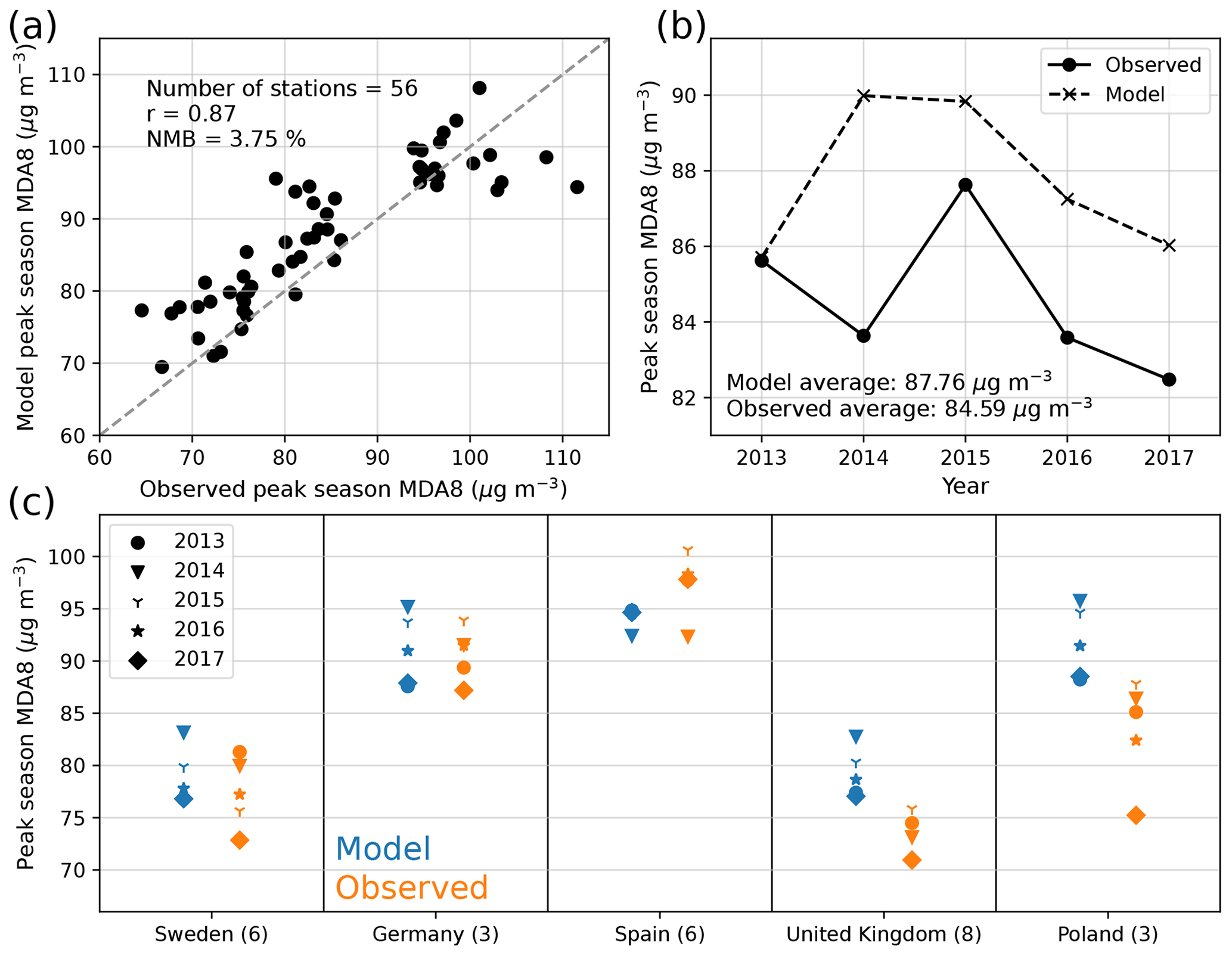
Figure 2 Modeled versus observed peak season MDA8 across Europe. Panel (a) shows 5-year-averaged values at each of the 56 stations, while panel (b) compares the annual values averaged over all stations. Panel (c) shows the yearly averages for Sweden, Germany, Spain, the United Kingdom, and Poland, with the number in brackets indicating the number of stations in each of the countries.

5 Results

While the focus in this section lies on peak season MDA8, results for other O₃ indicators are included in the Supplement, as referred to in the text. In addition, the following discusses a number of weighted averaging approaches for both health and vegetation O₃ indicators, with the different population and crop-area maps shown for reference in Fig. S3.

5.1 EMEP region peak season MDA8

Figure 3 shows a so-called cascade plot of the EMEP region population-weighted peak season MDA8 changes between the 2015 baseline and the 2050 CLE, MFR, and LOW scenarios. Here the population weighting is calculated using the Global Human Settlement Layer (GHSL) population distribution for the year 2015 (Schiavina et al., 2023), aggregated from its native 3 arcsec resolution to the regional EMEP grid and remaining unchanged for all scenarios. In Fig. 3, the impacts arising from NO_x, CO, and NMVOC precursor emission changes and from CH₄ are shown as separate cascade steps. In the cascades, the separate contributions arising from the EMEP region and ROW emission changes are also highlighted, as calculated using the model configurations described in Table 2. For example, the difference between the bs15_bs15ch4 and rowcle50_bs15ch4 simulations yields the change due to 2050 CLE precursor emission changes in the ROW region relative to the 2015 baseline, whereas the difference between the cle50_bs15ch4 and cle50_cle50ch4 simulations yields the change due to background CH₄ changes. The direction of the changes (increasing or decreasing) is illustrated using red arrows for the 2015 baseline to 2050 CLE scenario, highlighting that in this case increasing CH₄ concentrations lead to an increase in peak season MDA8. As noted in Sect. 4, the impact of global CH₄ emission changes is split into its EMEP and ROW region contributions based on the emission changes within these respective regions. In effect, the cascade plot thereby summarizes the impact of each of successive precursor and CH₄ change from the 2015 baseline down to the 2050 LOW scenario.

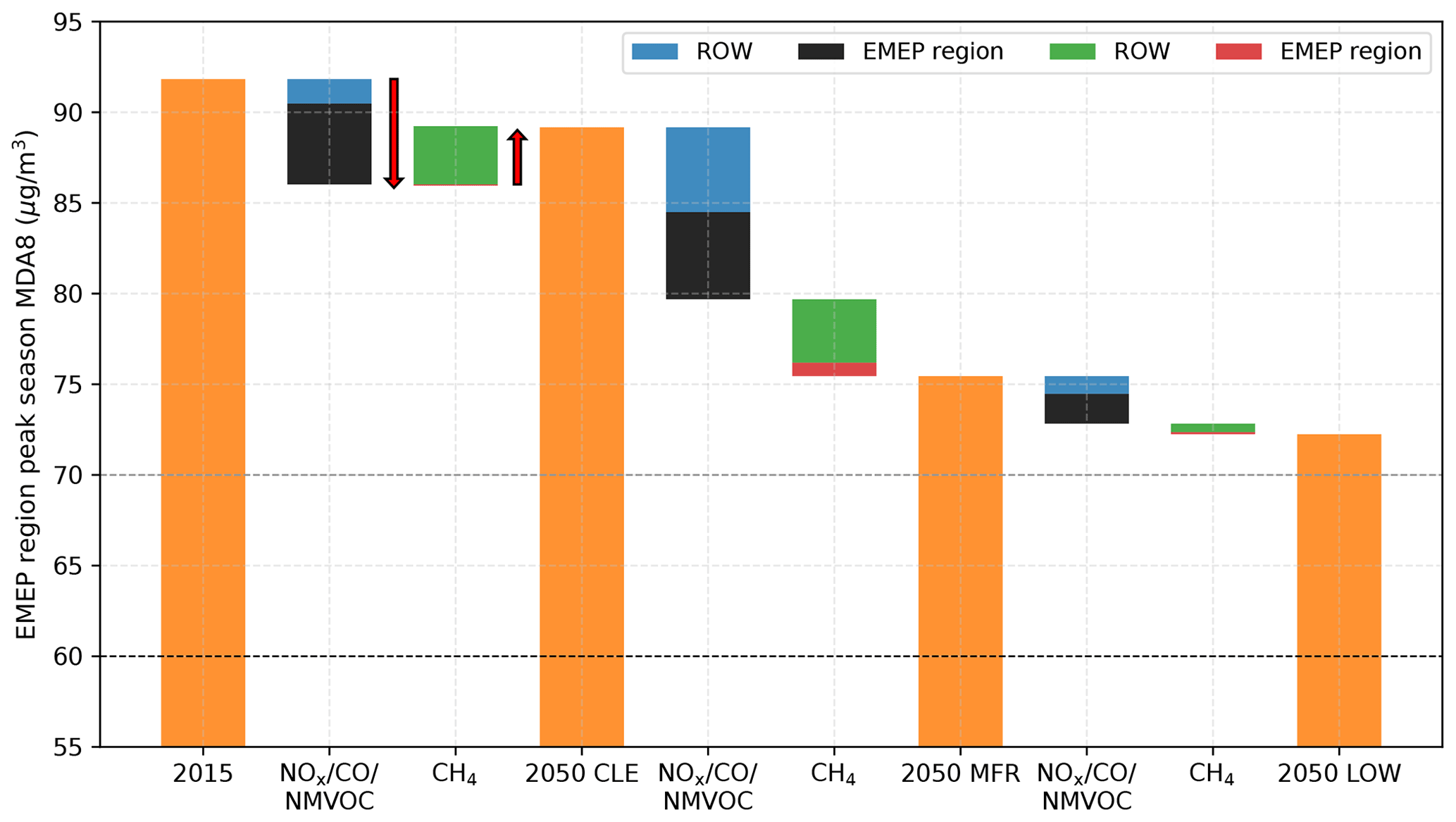
Figure 3 Cascade plot of the population-weighted EMEP region average peak season MDA8 scenario changes arising from NO_x, CO, and NMVOC emission changes within the EMEP (black) and ROW (blue) regions, as well as from background CH₄ changes arising from EMEP (red) and ROW (green) region emission changes. The dashed black and dashed gray horizontal lines denote guideline and interim WHO target values, respectively. Red arrows indicate the direction of the cascades from the 2015 baseline to 2050 CLE scenario for illustration, as described in the text.

Figure 3 shows that average peak season MDA8 concentrations are reduced from 91.8 to 89.2 µg m⁻³ between the 2015 baseline and 2050 CLE scenarios, resulting largely from a decrease in precursor emissions in the EMEP region (−4.5 µg m⁻³) and to a lesser extent in the ROW region (−1.4 µg m⁻³). However, these reductions are partially offset by an increase of 3.2 µg m⁻³ arising from increased background CH₄ concentrations, being almost entirely the result of increased CH₄ emissions in the ROW region. Going from the 2050 CLE to 2050 MFR scenario, the net reduction from 89.2 to 75.4 µg m⁻³ (−15.4 %) is split into three nearly equal parts arising from EMEP region precursor reductions, ROW precursor reductions, and background CH₄ reductions. The 2050 LOW scenario differs relatively little from the MFR, with roughly half of the change from 75.4 to 72.2 µg m⁻³ arising from further precursor emission reductions within the EMEP region. Cascade plots for the annual O₃ mean, SOMO35 (Sum of Ozone Means Over 35 ppb), and POD₃IAM_WH indicators, as discussed in Sect. 5.2, are shown in Figs. S4–S6.

Geographical distribution

To illustrate the impact of geographical location on the O₃ changes resulting from precursor and CH₄ emission changes, the difference in peak season MDA8 between the 2050 CLE and LOW scenarios is shown across the regional EMEP modeling domain in Fig. 4. Here the 2050 CLE to LOW impacts are calculated by combining the results from the 2050 CLE to 2050 MFR simulations with the 2050 MFR to 2050 LOW simulations described in Table 2. Figure 4a shows the change in peak season MDA8 resulting from the change to ROW LOW emissions. As expected, the ROW LOW impacts are most pronounced in the ROW countries within the regional modeling domain (e.g., North African countries). Nevertheless, countries along the southern border of the EMEP region as well as along the western coast of Europe also see reductions ranging from 5–15 µg m⁻³. The reductions along the western coast of Europe are likely the result of emission reductions in North America, with the associated O₃ perturbations carried over the Atlantic Ocean by the prevailing westerlies. Figure 4b shows that the impact of regional LOW emissions is largely centered on the EMEP region, ranging from approximately 5 µg m⁻³ in western Europe to 30 µg m⁻³ in western Balkan and EECCA countries. While local in nature, the impact of emission reductions in the EMEP and ROW regions can lead to increases of as much as 30 µg m⁻³ in large urban areas (as highlighted in Fig. 4b for Almaty, Kazakhstan), due to reductions in the titration effect of NO_x. The impact of background CH₄ reductions from 2236 to 1574 ppb is shown in Fig. 4c, with the latitudinal gradient likely to a large extent arising from the latitudinal variations in insolation. The resulting peak season MDA8 reductions amount to around 5 µg m⁻³ across the EMEP region.

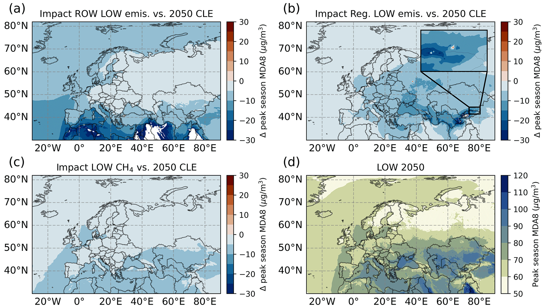
Figure 4 Reductions in peak season MDA8 achieved by 2050 ROW LOW (a) and EMEP region (b) precursor emission changes relative to the 2050 CLE scenario. Panel (b) also highlights the simulation results for Almaty, Kazakhstan. Panel (c) shows the reductions arising from the background CH₄ change from 2236 to 1574 ppb, while panel (d) shows the peak season MDA8 as simulated for the full 2050 LOW scenario. Note the difference in color scale for panel (d).

Figure 4d shows the results for the full 2050 LOW scenario, illustrating that peak season MDA8 concentrations fall below 60 µg m⁻³ over parts of northern Scandinavia, while ranging from 80 to 90 µg m⁻³ over northern Italy and Kazakhstan. In central Europe, concentrations typically range from 60–70 µg m⁻³, highlighting that the population-weighted WHO exposure guideline of 60 µg m⁻³ is, in fact, not met in any of the EMEP countries. However, the interim target of 70 µg m⁻³ is reached in a number of western European countries, such as the Netherlands, France, Germany, and the United Kingdom. The population-weighted LOW scenario concentrations for each of the individual countries in the EMEP region are shown in Fig. S7, along with their 2015 baseline and 2050 CLE and MFR concentrations. In addition, Fig. S8 follows that of Fig. 4 but instead compares the impacts of the LOW scenario against the 2015 baseline. For the latter, the impact of regional emission reductions is comparatively higher, while that of CH₄ changes is comparatively lower, consistent with the results shown in Fig. 3.

5.2 Other O₃ indicators

This section serves in part to provide reference to earlier studies by showing the scenario results for a range of other health and vegetation O₃ indicators. For example, earlier works have investigated the impact of precursor and CH₄ emission changes on (area-weighted) annual mean surface O₃ (O₃ mean) concentrations (Turnock et al., 2018; Jonson et al., 2018), while the SOMO35, fourth-highest annual MDA8, and summertime (JJA) average daily maximum O₃ concentrations have been used for health impact studies (Fleming et al., 2018). Furthermore, JJA average O₃ concentrations were used in the study of the climate impact on surface O₃ by Colette et al. (2015), as will be discussed in more detail in Sect. 6. For the impacts on vegetation, the growing-season accumulated phytotoxic ozone dose (POD_Y) uptake over a certain threshold value Y (nmol O₃ m⁻² s⁻¹) can induce reductions in crop and semi-natural biomass (Emberson, 2020; Mills et al., 2018). To this end, the integrated assessment modeling (IAM) vegetation-type-specific POD_Y indicators (POD_YIAM) serve as simplified risk assessment indicators for use in CTMs such as the EMEP model (Simpson et al., 2012, 2007), as also described in the UNECE mapping manual (UNECE, 2017). The POD₃IAM_WH indicator represents the cumulative growing-season (∼90 d) stomatal O₃ uptake for a generic temperate or boreal crop, being largely based on wheat (WH), and is used as an indicator for wheat yield loss (Pandey et al., 2023; Mills et al., 2018). In addition, the POD₁IAM_DF indicator is used in the risk assessment of reductions in annual living deciduous forest (DF) biomass growth (UNECE, 2017), having a ∼180 d growing season at 50° N.

Table 3 shows the absolute and percentage-change scenario results across the range of O₃ indicators for an extended range of (constructed) scenarios. For example, the “2015 base to 2050 MFR” scenario is constructed using the differences between the “2015 base to 2050 CLE” and the “2050 CLE to 2050 MFR” scenarios described in Table 2, while the “2050 CLE to 2050 LOW” scenario is constructed using the differences between the “2050 CLE to 2050 MFR” and “2050 MFR to 2050 LOW” scenarios (as described in Sect. 5.1.1). Likewise, the “2015 base to 2050 LOW” scenario is constructed using the differences between the “2015 base to 2050 CLE”, “2050 CLE to 2050 MFR”, and “2050 MFR to 2050 LOW” scenarios. Note that for peak season MDA8, the absolute numbers shown for the “2015 base to 2050 CLE”, “2050 CLE to 2050 MFR”, and “2050 MFR to 2050 LOW” scenarios correspond to those shown in Fig. 3. Furthermore, since the relative importance of CH₄ emission changes inside the EMEP region is small, Table 3 only includes the impact of global CH₄ changes. While health-related O₃ indicators are shown as population-weighted averages, the POD_Y indicators are shown as their respective vegetation-area-weighted averages (i.e., average values per square meter of vegetation, as illustrated in Fig. S3).

Table 3 Absolute and percentage-change (in brackets) scenario impacts across the EMEP region. Changes resulting from precursor emission changes in the EMEP (reg.) and ROW regions and from global CH₄ changes are shown relative to the scenario starting points. End values correspond to the weighted averages at each of the scenario end points.

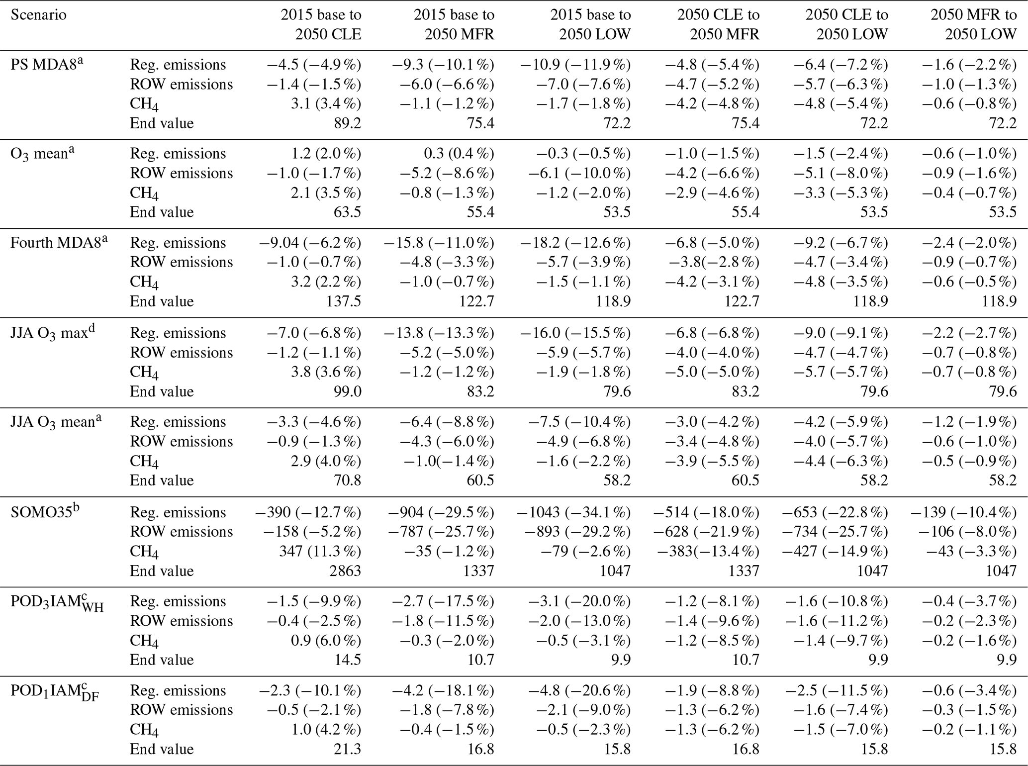
^a Population-weighted EMEP region average in µg m⁻³. ^b Population-weighted EMEP region average in ppb d. ^c Crop-area-weighted EMEP region average in mmol m⁻². ^d Population-weighted average converted from ppb to µg m⁻³ using the standard-atmosphere O₃ conversion factor of 1.96.

Table 3 illustrates that different uses of threshold values and time and length of averaging or accumulation periods lead to differences in the relative importance of precursor and CH₄ emission changes. For example, indicators most sensitive to O₃ concentrations during its peak photochemical production period (peak season MDA8, JJA O₃ max, JJA O₃ mean, and fourth-highest MDA8) are most strongly impacted by regional precursor emission reductions, especially when compared against the 2015 baseline scenario. In contrast, regional emission reductions are much less important for annual O₃, due to the competing effects of local wintertime NO_x titration. The importance of ROW emissions is, broadly speaking, proportional to the length of the averaging or accumulation period, while also being most relevant to the 2050 scenarios (i.e., 2050 CLE to MFR and LOW). For indicators employing a threshold value, the percentage-change impacts are proportional to the height of the threshold relative to the baseline (or background) value, which effectively determines the degree to which the natural background is filtered out. For example, the total percentage-change reduction from the 2015 baseline to 2050 LOW scenarios for the SOMO35, POD₃IAM_WH, and POD₁IAM_DF indicators amounts to 65.8 %, 40.3 %, and 31.9 %, respectively. While already implied in Fig. 3, Table 3 also shows that the impact of CH₄ emission reductions is most important relative to the 2050 CLE scenario and less so when compared against the 2015 baseline. However, O₃ mean is an exception to the latter, with CH₄ having the largest impact from the 2015 baseline to 2050 CLE scenario. Furthermore, CH₄ reductions contribute roughly one-third of the total reductions for each of the peak O₃ indicators for the 2050 CLE to 2050 MFR scenario, although this is closer to one-fourth for SOMO35 (25.1 %).

For the population-weighted O₃ indicators (i.e., all except those for vegetation), the corresponding area-weighted averages are shown in Table S2. While the results are generally consistent between the two weighted averaging approaches, indicators sensitive to peak O₃ concentrations are comparatively less impacted by regional precursor emission changes when calculated as area-weighted averages. However, the area-weighted impacts of regional precursor emission changes are considerably larger for annual O₃ mean, since NO_x titration effects in urban areas are weighted less heavily. For example, reducing regional emissions between the 2015 baseline to 2050 MFR scenarios sees a population-weighted O₃ mean reduction of 0.3 µg m⁻³ (0.4 %), while the corresponding area-weighted reduction amounts to 5.1 µg m⁻³ (7.7 %).

6 Discussion

In the current setup, the EMEP model is unable to capture the effects of future climate change on surface O₃ concentrations. This effect, often described as the O₃ climate penalty (e.g., Fu and Tian, 2019; Rasmussen et al., 2013), can affect surface O₃, for example, through climate-change-induced changes in water vapor concentrations and biogenic VOC emissions. For European land surfaces, Colette et al. (2015) estimated the 95 % confidence interval of the mid-century (2041–2070) surface JJA O₃ mean climate penalty to range from 0.44–0.64 ppb, based on an ensemble of 25 chemistry-climate model simulations. Compared to the JJA O₃ mean changes between the 2050 CLE and MFR scenarios shown in Table 3, amounting to 10.3 µg m⁻³ (or 5.2 ppb using the standard-atmosphere O₃ conversion factor of 1.96), the impact of the climate penalty on the results of the current work is expected to be small. Other climate uncertainties relate to the calculated CH₄ projections, with terrestrial soil emissions estimated to increase by 22.8±3.6 Tg CH₄ yr⁻¹ by the year 2100 in the SSP5-8.5 scenario (Guo et al., 2023). However, by the year 2050 and relative to the baseline natural emissions, estimated at 210 Tg yr⁻¹ in Sect. 3, the change in natural emissions is expected to be comparatively small and in part captured by increasing permafrost emissions as described in Sect. 3.

While constructing emission datasets based on a wide variety of information is by itself challenging (e.g., de Meij et al., 2024; Thunis et al., 2022), the emission scenarios employed in the current work are also inherently based on a number of socio-economic activity projections. In practice, the reliable quantification of the uncertainty on the input parameters to the GAINS model is itself considered the most uncertain element of the analysis (Amann et al., 2011). In light of this, the emission scenarios arguably represent the largest source of uncertainty in the current work, which is unavoidable and not directly quantifiable. Nevertheless, the GAINS model by design attempts to minimize the impact of uncertainties on policy-relevant model output to increase the robustness (i.e., the priorities and control needs between countries, sectors, and pollutants do not significantly change due to uncertainties in the model elements) of the emission control strategies (Amann et al., 2011).

6.1 O₃ production efficiency of CH₄

The CH₄ oxidation reaction that leads the production of O₃ depends on the availability of NO_x and OH (Crutzen et al., 1999). OH is produced through the photolysis of O₃ and subsequent reaction of O(1D) with water vapor (H₂O), with the majority of surface O₃ being produced by the photolysis of NO_x in VOC-rich environments. In addition, CO and VOCs (including CH₄) are net sinks of OH, creating a non-linear relationship between their atmospheric abundance and the O₃ production efficiency (OPE) of CH₄ (Isaksen et al., 2014). In the current work, the OPE is taken as the capacity of CH₄ to produce surface O₃ in the EMEP region. To investigate the impact of OPE on the calculated O₃ response, diagnostic EMEP model simulations are performed where background CH₄ concentrations are varied from 850 to 2600 ppb in 250 ppb steps, using the 2015 baseline and the 2050 CLE and LOW emission scenarios as the source of background precursor emissions. The resulting CH₄ impacts on peak season MDA8 are shown in Fig. 5, noting that the starting point of 850 ppb corresponds roughly to pre-industrial CH₄ concentrations. For simplicity, the simulations shown here are only calculated for the 2015 meteorological year but with otherwise the same model configuration (e.g., 6-month spin-up period) as described in Sect. 4.

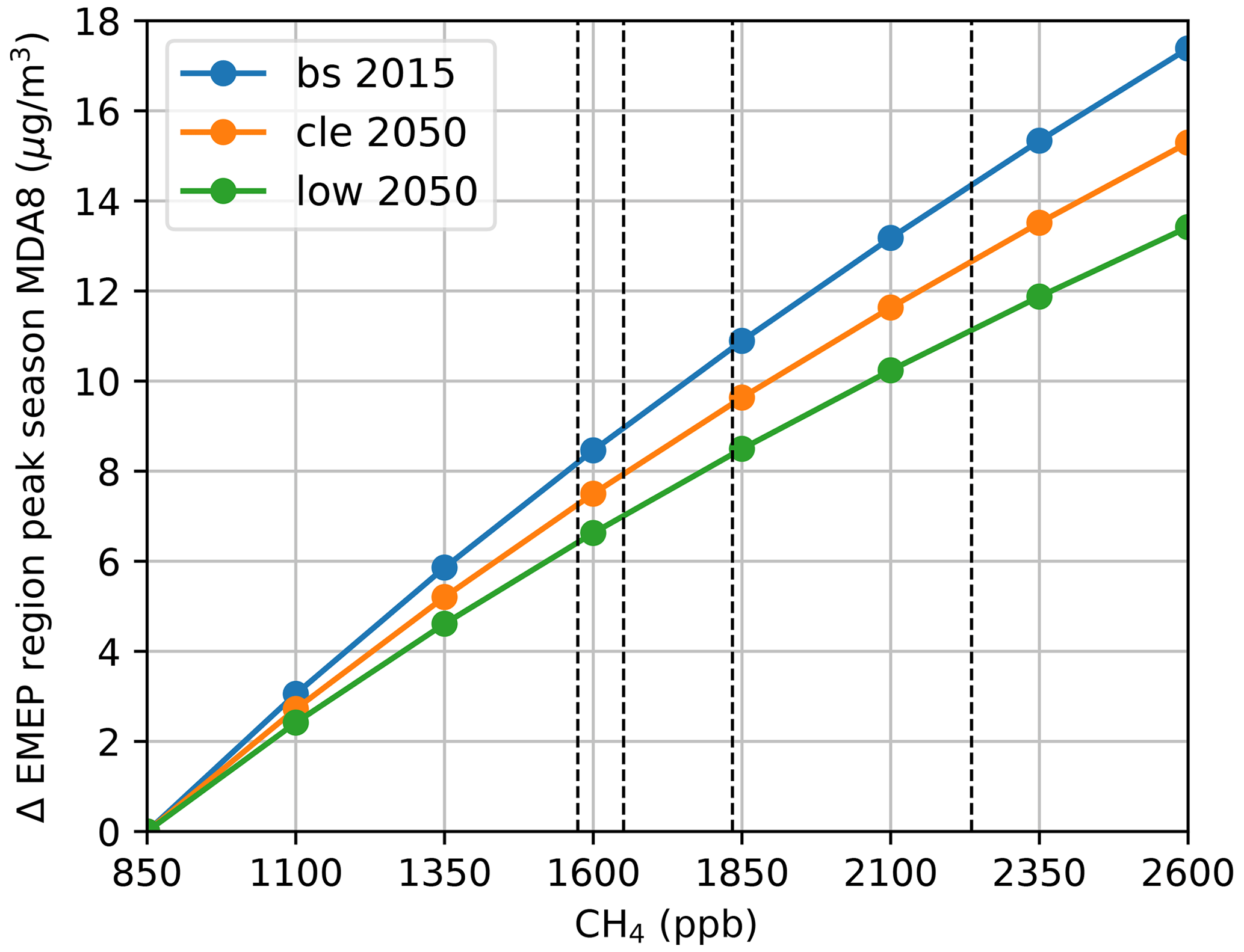
Figure 5 Change in the EMEP region population-weighted peak season MDA8 for background CH₄ concentrations ranging from 850 to 2600 ppb in 250 ppb intervals, relative to peak season MDA8 concentrations at 850 ppb CH₄. The impacts are calculated with the baseline 2015 and the 2050 CLE and LOW emission scenarios defined in Table 2. The dashed vertical lines mark the 2050 LOW, 2050 MFR, 2015 baseline, and 2050 CLE background CH₄ concentrations (1574, 1651, 1834, and 2236 ppb, respectively) as discussed in Sect. 3.

Figure 5 illustrates that the OPE is highest in the 2015 baseline scenario, when EMEP region NO_x emissions are also highest (Table 1). Regional NO_x emissions are reduced considerably already in the 2050 CLE scenario, while other emissions change relatively little. As a result, the OPE is a factor of 0.88 (12 %) smaller relative to the 2015 baseline across the range of CH₄ concentrations. Similarly, the OPE in the 2050 LOW scenario is a factor of 0.88 (12 %) lower than that of the 2050 CLE scenario and a factor of 0.78 (22 %) lower relative to the 2015 baseline scenario. The decrease from 2236 to 1574 ppb CH₄ between the 2050 CLE to 2050 LOW scenarios discussed in Sect. 3 leads to a reduction of peak season MDA8 by 5.4 and 4.7 µg m⁻³ when calculated with CLE and LOW precursor emissions, respectively. The reduction of 4.9 µg m⁻³ due to CH₄ as shown in Table 3, calculated with a combination of 2050 MFR and 2050 LOW precursor emissions, therefore depends relatively less on the choice of background precursor emissions and more so on the background CH₄ changes themselves.

Figure 5 furthermore illustrates that the peak season MDA8 response is approximately linear in the range of CH₄ concentrations relevant to the current work, supporting the approach of splitting the O₃ impacts based on the separate emission changes within the EMEP and ROW regions. Another corollary is that the contribution of anthropogenic background CH₄ to total peak season MDA8 can be calculated to amount to approximately 10.7 (11.6 %), 12.7 (14.2 %), and 6.4 (8.9 %) µg m⁻³ in the 2015 baseline, 2050 CLE, and 2050 LOW scenarios, respectively. Here the percentage contributions are based on the scenario totals shown in Fig. 3 and Table 3. Recognizing that the MFR and LOW precursor emission scenarios are nearly identical except for CH₄ emissions, the anthropogenic CH₄ contribution calculated for the 2050 MFR scenario (1651 ppb) amounts to 7.0 µg m⁻³ (9.3 %).

6.2 Comparison to previous studies

While important for placing the results in context, comparing the results of the current work to earlier studies can be challenging, for example, due to differences in source-receptor area definitions, model configuration, weighted averaging approach, and emission scenarios. Nevertheless, while the modeling setup of Belis and Van Dingenen (2023) is different in that linear pre-calculated transfer coefficients of the TM5-FAst Scenario Screening Tool (TM5-FASST) are used in place of full CTM simulations, our calculated EMEP region total peak season MDA8 exposure reduction by 15 % between the 2050 CLE and MFR scenarios is consistent with their 16 % reduction found across the entire UNECE region (including North America) based on CLE and MFR scenarios from the ECLIPSE version 6b dataset. However, in our calculations the total 2050 MFR anthropogenic CH₄ contribution amounts to 7.0 µg m⁻³ (or 3.5 ppb using the standard-atmosphere O₃ conversion factor of 1.96), which is lower than their estimate of ∼5 ppb (based on their Fig. S4). This can largely be reconciled considering that our estimate was calculated with the 2050 LOW scenario as the source of background precursor emissions, while theirs is based on O₃ sensitivities calculated from a 2010 baseline emission scenario. When using the 2015 baseline emission scenario as the source of background precursor emissions in our calculations, the total 2050 MFR anthropogenic CH₄ contribution amounts to 9.0 µg m⁻³, or 4.5 ppb, which is more comparable.

In the work of Turnock et al. (2018), the box model described in Holmes et al. (2013) is used to estimate the 2050 CLE and MFR CH₄ concentrations to amount to 2361 and 1420 ppb, respectively. They further estimate the 2050 CLE increase in CH₄ to contribute 1.6 ppb to annual mean area-weighted O₃ across Europe relative to a 2010 baseline concentration of 1798 ppb, based on the parameterized response of 14 models. While the latter is higher than our estimate of 1.1 ppb for the EMEP region (Table S3, using the standard-atmosphere O₃ conversion factor of 1.96), our results find a more comparable contribution of 1.4 ppb when the response is calculated as the European area-weighted average following the land-area definition of Turnock et al. (2018). However, in our results the 2050 CLE and MFR ensemble mean CH₄ concentrations amount to 2236 and 1651 ppb, respectively, with the total difference between the CLE and MFR scenarios therefore being 403 ppb (or 43 %) less than that of Turnock et al. (2018). While this may in part be due to their MFR scenario diverging from the CLE from 2020 rather than 2025 onwards, it nevertheless highlights the importance of the methodology used to estimate CH₄ concentrations, as the cumulative difference between scenarios can quickly diverge. The difference in CH₄ estimates also has implications for the impact of the 2050 MFR emissions relative to the baseline, which in our analysis (−183 ppb) is around half that determined by Turnock et al. (2018) (−378 ppb).

6.3 Air pollution and global warming co-benefits

While a detailed discussion is beyond the scope of the current work, the global mean temperature change relative to the reference period of 1986–2005, as calculated for the 600-ensemble mean and 5 %–95 % range using the MAGICC7 model in Sect. 3, amounts to 2.21 [1.61–2.94], 2.02 [1.45–2.74], and 1.92 [1.33–2.67] °K for the 2050 CLE, MFR, and LOW scenarios, respectively. In the LOW-CH₄ scenario, where CH₄ emissions follow the LOW scenario while all other emissions follow that of the CLE, this change amounts to 2.03 [1.47–2.74] °K. Thus illustrating that around two-thirds of the global warming reduction between the 2050 CLE (SSP2-4.5 GHGs) and LOW (SSP1-2.6 GHGs) scenarios can be achieved by solely reducing CH₄ emissions.

7 Conclusions

This work investigates the impact of CH₄ and other precursor emissions on surface O₃ concentrations in the EMEP region for the CLE, MFR, and LOW emission scenarios up to the year 2050. In the CLE scenario, background CH₄ concentrations are projected to increase by 402 ppb (22 %) relative to 2015 baseline concentrations, while they are reduced by 183 ppb (−10 %) in the MFR scenario. By 2050, the difference between the MFR and CLE scenarios therefore amounts to 585 ppb (or 26.1 % less in the MFR compared to the CLE), while the LOW scenario achieves a modest further 77 ppb reduction. The MFR CH₄ reductions lead to a peak season MDA8 exposure reduction of 4.2 µg m⁻³ (4.8 %) relative to the 2050 CLE case, contributing around one-third of the total peak season MDA8 reduction (13.7 µg m⁻³, or 15.4 %). The other two-thirds are split almost equally between the impact of other precursor (NO_x, CO, NMVOCs) emission reductions in the EMEP and ROW regions, respectively. As for CH₄, the impact of further abatement policies for the other precursor emissions is comparatively small in the LOW scenario. Focusing therefore on the comparison between the 2050 CLE and MFR scenarios, our results highlight that reducing CH₄ emissions has the potential to lead to substantial peak season MDA8 reductions, having a similarly strong effect to the reduction of other precursor emissions within the EMEP region. The CH₄ reductions are, however, almost entirely the result of and can only be achieved by CH₄ emission reductions outside of the EMEP region. Moreover, relative to the 2015 baseline, the increasing CH₄ concentrations in the 2050 CLE scenario partly offset (+3.1 µg m⁻³) the peak season MDA8 reductions achieved by the CLE reductions of other precursor emissions in the EMEP region (−4.5 µg m⁻³). This highlights that simultaneous reductions in CH₄ emissions help avoid offsetting the air pollution benefits already achieved by the (regional) CLE precursor emission reductions, while also playing an important role in bringing air pollution further down beyond the 2050 CLE scenario.

In terms of the total reductions, the 2050 MFR scenario brings the EMEP region average peak season MDA8 exposure down from 89.2 to 75.4 µg m⁻³ relative to the CLE, against a 2015 baseline exposure of 92.0 µg m⁻³. Nevertheless, in the MFR scenario the majority of countries in the EMEP region (38 out of 49) are projected to stay above the interim WHO exposure target of 70 µg m⁻³. While the more stringent emission policies of the LOW scenario reduce the number of countries to 30, it still highlights the difficulties in reaching WHO guideline values, given also that even in the LOW scenario none of the countries fall below the 60 µg m⁻³ WHO limit. However, our results may be regarded as somewhat of an upper estimate, as the comparison against observations across Europe found the model to overestimate peak season MDA8 by 3.8 % (3.2 µg m⁻³) on average in the 2015 baseline emission scenario.

While the current work focuses on the peak season MDA8 indicator, the scenario results are also discussed for a range of other health and vegetation O₃ indicators. These results find that the relative importance of CH₄ and other precursor emission reductions depends on the choice of indicator and to some extent on the spatial averaging approach (area or population weighted). Nevertheless, O₃ indicators emphasizing peak O₃ concentrations (e.g., SOMO35, JJA O₃ max, fourth MDA8) yield results largely consistent with those for peak season MDA8 in terms of the relative importance of the different emission changes. The scenario percentage-change impacts can vary considerably between the different indicators, being mostly dependent on the extent to which a threshold value applies. For example, the total reduction between the CLE and MFR scenarios for the SOMO35 health indicator and the POD₃IAM_WH vegetation indicator amounts to 53.3 % and 26.2 %, respectively, compared to a 15.4 % total reduction for peak season MDA8.

The current work also highlights that reducing CH₄ emissions achieves considerable global warming reductions, with solely reducing CH₄ emissions achieving roughly two-thirds of the possible temperature reduction between the full 2050 CLE (SSP2-4.5 GHGs) and LOW (SSP1-2.6 GHGs) scenarios. However, as for the CH₄ air pollution benefits, the global warming reductions are almost entirely the result of CH₄ emission reductions outside of the EMEP region.