Interannual variations in the Δ(¹⁷O) signature of atmospheric CO₂ at two mid-latitude sites suggest a close link to stratosphere–troposphere exchange

Δ(¹⁷O) measurements of atmospheric CO₂ have the potential to be a tracer for gross primary production and stratosphere–troposphere mixing. A positive Δ(¹⁷O) originates from intrusions of stratospheric CO₂, whereas values close to −0.21 ‰ result from the equilibration of CO₂ and water, which predominantly happens inside plants. The stratospheric source of CO₂ with high Δ(¹⁷O) is, however, not well defined in the current models. More, and long-term, atmospheric measurements are needed to improve this. We present records of the Δ(¹⁷O) of atmospheric CO₂ obtained with laser absorption spectroscopy from Lutjewad in the Netherlands (53°24^′ N, 6°21^′ E) and Mace Head in Ireland (53°20^′ N, 9°54^′ W) that cover the period 2017–2022. The records are compared with a 3-D model simulation, and we study potential model improvements. Both records show significant interannual variability of up to 0.3 ‰. The total range covered by smoothed monthly averages from the Lutjewad record is −0.34 ‰ to −0.12 ‰, which is significantly higher than the range of −0.20 ‰ to −0.17 ‰ for the model simulation. The 100 hPa 60–90° N monthly-mean temperature anomaly was used as a proxy to scale stratospheric downwelling in the model. This strongly improves the correlation coefficient of the simulated and observed year-to-year Δ(¹⁷O) variations over the period 2019–2021 from 0.40 to 0.82. As the Δ(¹⁷O) of atmospheric CO₂ seems to be dominated by stratospheric influx, its use as a tracer for stratosphere–troposphere exchange should be further investigated.

1 Introduction

Stable-isotope measurements of atmospheric CO₂ have been a great asset to carbon cycle research (Mook et al., 1983; Keeling et al., 1984; Ciais et al., 1997; Welp et al., 2011; Carlstad and Boering, 2023). As different isotopologues of CO₂ have the same chemical properties and will be incorporated in the same carbon cycle fluxes, their difference in mass can result in the preferred uptake or emission of the lighter or heavier isotopologues for certain processes. This is known as kinetic fractionation (Young et al., 2002). Another form of fractionation is equilibrium fractionation, in which isotopes of different substances at chemical equilibrium are partially separated (Young et al., 2002). Fractionation will thus influence the isotope composition of atmospheric CO₂ and, together with CO₂ amount fraction measurements, the isotope composition of atmospheric CO₂ can help to disentangle carbon sources and sinks (Peters et al., 2018; Welp et al., 2011; Hofmann et al., 2017; Keeling et al., 2005; Laskar et al., 2016). Isotope composition is generally expressed relative to an internationally recognized reference material using the delta notation:

$$\begin{array}{}\text{(1)}& \mathit{\delta }{(}^{*}A)={\displaystyle \frac{{[}^{*}{A}_{\text{s}}]/[A_{\text{s}}]}{{[}^{*}{A}_{\text{r}}]/[A_{\text{r}}]}}-\mathrm{1},\end{array}$$

in which A is the atom (for CO₂, this is C or O), the superscript ^* indicates the rare isotope (13 for C; 17 or 18 for O), the A without ^* is the most abundant isotope (12 for C, 16 for O), and the subscripts “s” and “r” indicate the sample and reference, respectively. Delta values are usually expressed in per mille, indicated by the ‰ symbol, as natural variation is very small. Applications of δ(¹³C) and δ(¹⁸O) measurements of atmospheric CO₂ are numerous and have proven to be of great value for the identification and quantification of sources and sinks of atmospheric CO₂ (Roeloffzen et al., 1991; Ciais et al., 1995; Rayner et al., 2008) and for the description of the air-mixing dynamics of the troposphere and stratosphere (Assonov et al., 2010).

The relation between δ(¹⁷O) and δ(¹⁸O) resulting from the kinetic and equilibrium fractionation processes as described above is relatively constant and can be described by

$$\begin{array}{}\text{(2)}& \ln \left(\mathit{\delta }{(}^{\mathrm{17}}\mathrm{O}\right)+\mathrm{1})=\mathit{\theta }\ln (\mathit{\delta }{(}^{\mathrm{18}}\mathrm{O})+\mathrm{1}),\end{array}$$

with θ ranging between 0.5 and 0.53, depending on the dominant fractionation process studied (Adnew et al., 2022). Δ(¹⁷O) can be calculated from the δ(¹⁸O) and δ(¹⁷O) values or the triple oxygen isotope composition. This is the expression of the deviation from a constant relation between the δ(¹⁸O) and δ(¹⁷O) values, which can be described using an arbitrary value defined as λ. Throughout this study, we use a λ value of 0.528, the reference line defined from measurements of δ(¹⁸O) and δ(¹⁷O) values in natural waters (Meijer and Li, 1998), which is also written as λ_RL and was recommended as the consensus value to express Δ(¹⁷O) in Miller and Pack (2021).

$$\begin{array}{}\text{(3)}& \mathrm{\Delta }{(}^{\mathrm{17}}\mathrm{O})=\ln (\mathit{\delta }{(}^{\mathrm{17}}\mathrm{O})+\mathrm{1})-{\mathit{\lambda }}_{\mathrm{RL}}\ln \left(\mathit{\delta }{(}^{\mathrm{18}}\mathrm{O}\right)+\mathrm{1})\end{array}$$

The Δ(¹⁷O) of tropospheric CO₂ is mainly influenced by two processes: (1) the intrusion of stratospheric CO₂ carrying a strongly deviating (Δ(¹⁷O) ≫0) signal (Thiemens et al., 1995; Boering et al., 2004; Kawagucci et al., 2008; Lämmerzahl et al., 2002) due to the exchange of CO₂ and O₃ via O(¹D) (Yung et al., 1991) and (2) the equilibration of tropospheric CO₂ with water, resulting in CO₂ with a Δ(¹⁷O) of −0.21 ‰ (Hoag et al., 2005; Barkan and Luz, 2012), providing the water has a Δ(¹⁷O) of zero. This equilibration mainly occurs in plant leaves due to the presence of the enzyme carbonic anhydrase, which speeds up the equilibration process of CO₂ and water by an order of magnitude such that the oxygen isotope composition of CO₂ which diffuses from the leaves back into the atmosphere (about two-thirds of the total uptake of CO₂ by plants Adnew et al., 2023) is largely in equilibrium with that of the leaf water (Francey and Tans, 1987).

Measurements of stable isotopes are traditionally done with isotope ratio mass spectrometry (IRMS); however, the measurement of the δ(¹⁷O) of CO₂ is not straightforward with this method due to isobaric interferences from the ¹³C¹⁶O₂ and the ¹²C¹⁶O¹⁷O isotopologues. These measurements can therefore only be done by measuring ion fragments, requiring a higher mass resolution and a very-high-sensitivity IRMS system, or by O₂–CO₂ exchange, a sample preparation procedure that is very labour intensive (Mahata et al., 2013; Adnew et al., 2019). The latter method has acquired a precision of higher than 0.01 ‰ for measurements of Δ(¹⁷O) (Adnew et al., 2019; Liang et al., 2023). Laser absorption spectroscopy measurements of Δ(¹⁷O) (along with δ(¹³C) and δ(¹⁸O)) in pure CO₂ (Stoltmann et al., 2017) and directly on CO₂ in air (Steur et al., 2021; Hare et al., 2022; Perdue et al., 2022; Bajnai et al., 2023) now reach precisions close to or higher than those of IRMS measurements. Laser absorption spectroscopy uses the absorption peaks of three different isotopologues of CO₂ to define the triple oxygen isotope composition. Therefore, the measurements can be conducted directly on air mixtures containing CO₂ at atmospheric amount fractions. This strongly reduces the preparation time for Δ(¹⁷O) measurements, providing the potential to set up large(r)-scale measurement programmes to evaluate the potential of the Δ(¹⁷O) of atmospheric CO₂ for carbon cycle and atmospheric research. From 2017, the Stable Isotopes of CO₂ Absorption Spectrometer (SICAS), which measures the δ(¹³C), δ(¹⁸O) and Δ(¹⁷O) of atmospheric CO₂, has been used at the Centre for Isotope Research (CIO) in Groningen. Air samples from two atmospheric measurement stations, Lutjewad and Mace Head, located on the north coast of the Netherlands and the west coast of Ireland, respectively, were measured regularly at the CIO for their trace-gas amount fractions and stable-isotope compositions over the period 2017–2022. We elaborately checked the quality of the measurements by considering the full uncertainty budget as well as comparing atmospheric sample measurements with results derived from IRMS measurements.

In this paper, multi-year records of Δ(¹⁷O) measurements conducted using laser absorption spectroscopy are presented along with the CO₂ amount fraction and δ(¹³C) and δ(¹⁸O) measurements. Observational data on the triple oxygen isotope composition of tropospheric CO₂ have scarcely been reported in the literature so far. Earlier records of Δ(¹⁷O) measurements of atmospheric CO₂, all conducted using IRMS, from Jerusalem (Israel) (Barkan and Luz, 2012), La Jolla (USA) (Thiemens et al., 2014), Taipei (Taiwan) (Liang and Mahata, 2015), cruises on the South China Sea (Liang et al., 2017), the Palos Verdes Peninsula (USA) (Liang et al., 2023), and Göttingen (Germany) (Hofmann et al., 2017) – the only close-to-mid-latitude measurement site – have been published. Göttingen, located in central Germany about 400 km southwest of the Lutjewad atmospheric measurement station, has a similar although more continental climate, and its record is therefore most comparable to Lutjewad when continental air masses are sampled.

The Δ(¹⁷O) record for Lutjewad is compared to model simulations of the Δ(¹⁷O) signal of the atmospheric CO₂ in Lutjewad as described in Koren et al. (2019). Finally, an outlook is given on how the SICAS, or laser absorption spectroscopy in general, can be used to collect data relevant for studying the Δ(¹⁷O) of atmospheric CO₂ in the future.

2 Methods

2.1 Sampling sites

The Lutjewad atmospheric measurement station is located on the northern coast of the Netherlands, at 53°24^′ N, 6°21^′ E. Since 2018, Lutjewad station has been a class 2 station in the European Integrated Carbon Observation System (ICOS) network. The station is located directly behind the Wadden Sea dike, in a flat, rural area. The location allows the sampling of marine (background) air with northern winds and continental air (50 % of the time) with southerly winds. Air is pumped from the top of the 60 m high tower via inlets connected to a series of tubing towards a laboratory building containing the instruments for continuous monitoring and an automated flask sampling system. The flasks used in our flask sampling network are 2.3 L volume glass flasks with two Louwers Hapert Viton sealed valves. The automated flask sampler is able to fill up to 20 flasks at ambient pressure and is set at a typical frequency of one flask sample every 3 d, taken at 12:00 local time. Each flask is flushed for 1 h with cryogenically dried sample air to a dew point below −50 °C before the sampler closes it and continues to flush the next flask (Neubert et al., 2004). Samples from the period 2017–2022 were used for this study. During this period, the flask sampling system occasionally failed, causing periods of sparser sampling, especially during 2019 and the beginning of 2022.

The atmospheric measurement station Mace Head, (operated by the National University of Ireland, Galway) is located along the west coast of Ireland (53°20^′ N, 9°54^′ W) on a cliff at 17 m above sea level. When the wind direction is from the west to the southwest, well-mixed air masses from the North Atlantic cross the station (Stanley et al., 2018). These wind conditions occur about half of the time, and during these periods Mace Head can be used as a background station for Northern Hemisphere background air. Once a week, when the air masses at the site are representative for Northern Hemisphere background air, a flask sample is taken at the Mace Head station from a 23 m high tower and sent to the CIO for the analysis of trace-gas measurements and the stable-isotope composition of CO₂. From the beginning of 2019 onwards, we started to routinely measure the Mace Head flask samples on the SICAS.

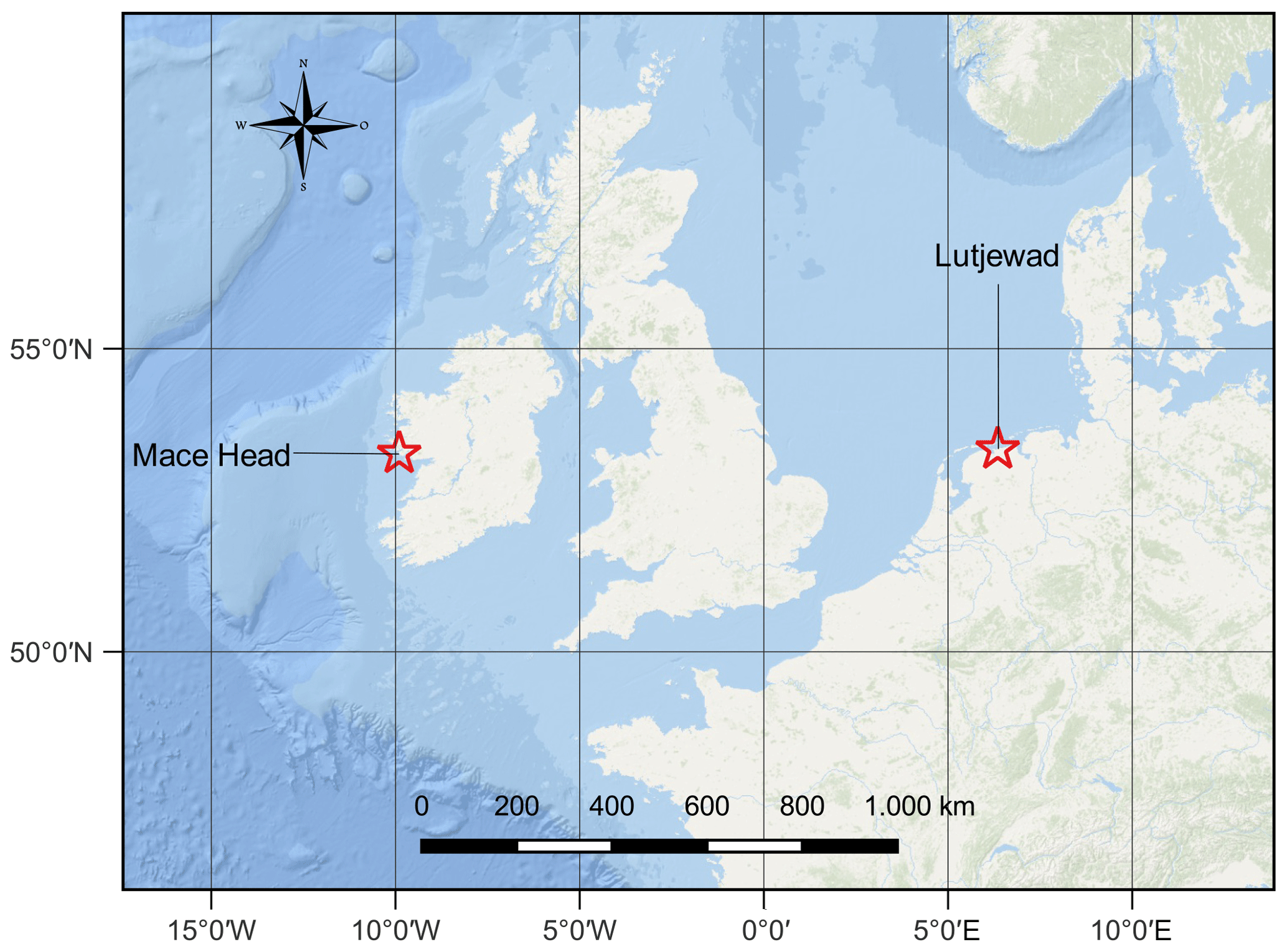
Figure 1 Locations of the Lutjewad and Mace Head atmospheric measurement stations on a map (created by Tim Maalderink)

2.2 Trace-gas amount fraction measurements

Continuous measurements of CO₂, CH₄ and CO amount fractions were conducted at the Lutjewad station with cavity ring-down spectrometry (CRDS) (G2401 series, Picarro) from 2013 on. Flask samples were measured for the same species at the CIO laboratory, with the majority of those measurements conducted using a customized HP Agilent HP6890N gas chromatograph (HPGC) equipped with a methanizer and a flame ionization detector (Worthy et al., 2003; van der Laan et al., 2009). This system was in operation until mid-2021, after which we used CRDS for flask analyses. All CO₂ measurements were calibrated using whole dry-air working standards made in-house and linked to the World Meteorological Organization X2019 scale, while CH₄ measurements were linked to the X2004A scale and CO measurements were linked to the X2014A scale. Continuous CRDS measurements are shown as hourly means, and therefore the standard deviations can vary considerably, depending on the stability of the trace-gas amount fractions in the atmosphere during the measurement period. Flask measurements on the HPGC show typical measurement precisions of <0.1 µmol mol⁻¹, <1.0 nmol mol⁻¹ and <1.0 nmol mol⁻¹ for CO₂, CH₄ and CO, respectively. In addition, CRDS measurements of the flask samples show typical precisions of <0.1 µmol mol⁻¹, <0.7 nmol mol⁻¹ and <2.0 nmol mol⁻¹ for CO₂, CH₄ and CO, respectively. The scale uncertainty is ±0.07 µmol mol⁻¹ for CO₂, ±1 nmol mol⁻¹ for CH₄ and ±2 nmol mol⁻¹ for CO.

2.3 Stable-isotope measurements

Stable-isotope composition measurements are conducted directly on atmospheric air samples, using the same flasks collected for the trace-gas amount fraction measurements, with the SICAS, a dual-laser spectrometer (CW-IC-TILDAS-D, Aerodyne) operating in the mid-infrared region. The measurement procedure is extensively described in Steur et al. (2021), and the calibration procedure and the determination of the combined uncertainty is described in Chapter 5 of Steur (2023), so we only briefly explain them here. The combined uncertainty is determined for all SICAS measurements, and includes the measurement uncertainty, the repeatability and residual of the measurement series, and the uncertainty introduced as a result of the calibration procedure. All these components are explained below.

Measurements are performed in static mode and are repeated for nine aliquots per sample. The gas consumption per aliquot is 20 mL, so measuring one sample requires 180 mL of air. A drift correction is carried out by measuring the working gas (a reference: a high-pressure cylinder containing air with a known CO₂ amount fraction and CO₂ stable-isotope composition), alternating with every aliquot measurement. This should correct the instrumental drift, which has also been identified in similar measurement systems and is caused by temperature variations (Hare et al., 2022; Bajnai et al., 2023). The temperature typically does not vary more than 0.05 °C within one measurement series covering 12 h for the SICAS (Steur et al., 2021). The standard error of the drift-corrected aliquot measurements per sample is the measurement uncertainty. The average measurement uncertainties are 0.010 ‰, 0.009 ‰ and 0.019 ‰ for δ(¹³C), δ(¹⁸O) and Δ(¹⁷O), respectively (Steur, 2023).

Besides the flask samples and the working gas, we include at least three other references in a measurement series (measurement cycle); these are all measured four times throughout the measurement series. At least two of these references, together with the working gas, are used for the calibration of the measurements. One of the references serves as a quality control (QC) measurement, or a known unknown, and is not used to determine the calibration curves but as an indicator of the quality of the measurement series. The repeatability of the measurement series is calculated as the standard deviation of the four QC measurements. We observe an average repeatability of 0.03 ‰, 0.02 ‰ and 0.04 ‰ for δ(¹³C), δ(¹⁸O) and Δ(¹⁷O) per measurement series, respectively (Steur, 2023). The residual per measurement series is calculated as the average of the calibrated QC measurements minus the known value of the QC.

The calibration method used for a sample measurement depends on the CO₂ amount fraction of the sample relative to the references. The uncertainty introduced by the calibration is highly dependent on the difference, in CO₂ amount fraction, of a sample from the closest reference as well as the difference between the references (Steur, 2023). We calibrate with the reference cylinders only, instead of having an on-line mixing facility where the reference and sample CO₂ amount fractions can be matched (Perdue et al., 2022; Bajnai et al., 2023). Therefore, samples that fall outside the range of the CO₂ amount fraction that is covered by our reference cylinders will have higher uncertainties.

We use two different calibration methods: the isotopologue method (IM) and the ratio method (RM) (Steur et al., 2021), and varying uncertainties are assigned to the sample measurements, depending on the difference in CO₂ amount fraction between the sample and the references. The IM is used when the sample is within the CO₂ amount fraction range of the references. For the IM, quadratic calibration curves are determined from the measured isotopologue amount fractions and known amount fractions of a minimum of three references, including the working gas. The calibrated isotopologue amount fractions of the samples are subsequently used for the calculation of the delta values. Ideally, the sample is bracketed closely in CO₂ amount fraction by the references. When the difference from the nearest reference is 15 µmol mol⁻¹ or lower, uncertainties of 0.03 ‰ for δ(¹³C) and δ(¹⁸O) and 0.05 ‰ for δ(¹⁷O) and Δ(¹⁷O) are introduced. When the difference is higher than 15 µmol mol⁻¹, an uncertainty of 0.09 ‰ is introduced for δ(¹³C) and δ(¹⁸O), and uncertainties of 0.11 and 0.10 ‰ are introduced for δ(¹⁷O) and Δ(¹⁷O), respectively.

When the sample falls outside of the CO₂ amount fraction range of the references, the RM is used. A linear correction of the measured delta values, which depends on the CO₂ amount fraction, is applied. In this way, a correction for the introduced CO₂ amount fraction dependency of the measured delta values is applied. This correction is needed as a result of measured and assigned isotopologue amount fraction dependencies with a non-zero intercept (Griffith et al., 2012). The uncertainty increases with extrapolation distance (the difference between the sample and the nearest reference in CO₂ amount fraction) when the sample falls outside the CO₂ amount fraction range of the references. The introduced uncertainty (u) in ‰ due to the extrapolation distance (Δy(CO₂)) in µmol mol⁻¹ is determined according to the following equations:

$$\begin{array}{}\text{(4)}& \begin{array}{rl}& u_{\mathit{\delta }{(}^{\mathrm{13}}\mathrm{C})}/\mathrm{‰}=\mathrm{0.0042}\mathrm{\Delta }y\left({\mathrm{CO}}_{\mathrm{2}}\right)/\left(\mathrm{\mu }\mathrm{mol}{\mathrm{mol}}^{-\mathrm{1}}\right)+\mathrm{0.03}\\ & u_{\mathit{\delta }{(}^{\mathrm{18}}\mathrm{O})}/\mathrm{‰}=\mathrm{0.0054}\mathrm{\Delta }y\left({\mathrm{CO}}_{\mathrm{2}}\right)/\left(\mathrm{\mu }\mathrm{mol}{\mathrm{mol}}^{-\mathrm{1}}\right)+\mathrm{0.03}\\ & u_{\mathit{\delta }{(}^{\mathrm{17}}\mathrm{O})}/\mathrm{‰}=\mathrm{0.0063}\mathrm{\Delta }y\left({\mathrm{CO}}_{\mathrm{2}}\right)/\left(\mathrm{\mu }\mathrm{mol}{\mathrm{mol}}^{-\mathrm{1}}\right)+\mathrm{0.05}\\ & u_{\mathrm{\Delta }{(}^{\mathrm{17}}\mathrm{O})}/\mathrm{‰}=\mathrm{0.0042}\mathrm{\Delta }y\left({\mathrm{CO}}_{\mathrm{2}}\right)/\left(\mathrm{\mu }\mathrm{mol}{\mathrm{mol}}^{-\mathrm{1}}\right)+\mathrm{0.05}.\end{array}\end{array}$$

The introduced uncertainties are all based on empirical data from reference measurements taken over a period of 2 to 3 years, as described in Chapter 5 of Steur (2023). As the Lutjewad and Mace Head stable-isotope records presented in this study are measured only on the SICAS, scale uncertainties are not included in the combined uncertainties of the measurements. To avoid showing irrelevant results, only values with a combined uncertainty lower than 0.1 ‰ will be included in the results of the stable-isotope measurements. The highest reference included in the calibration for the records has a CO₂ amount fraction of 424.54 µmol mol⁻¹, so the consequence is that samples with CO₂ amount fractions higher than 441.2, 437.5 and 436.4 µmol mol⁻¹ are excluded from the δ(¹³C), δ(¹⁸O) and Δ(¹⁷O) records, respectively. Especially at the Lutjewad station, it is not uncommon to sample air with this range of CO₂ amount fractions during winter. This will hence lead to a bias, as results for local or regional events leading to elevated CO₂ amount fractions that were captured in the flask records are not included in the results. Extending the CO₂ amount fraction range of our reference cylinders will improve the measurement precision of samples with elevated CO₂ amount fractions and will extend the range of CO₂ amount fractions that can be shown in the results. A way to prevent the need for a high number of reference cylinders to be included at all times is to make the selection of references more dynamic. As sample measurements are always alternated with a working-gas measurement, it is possible to do a one-point calibration immediately after a sample is measured. In this way, it is possible to select the ideal set of references to calibrate the samples based on the CO₂ amount fractions derived from the one-point calibration. This saves reference gas and reduces the measurement time of a measurement series.

Table 1 Natural-air references used for the calibration of the stable-isotope measurements presented in this study. δ(¹³C) and δ(¹⁸O) values as measured at the BGC-IsoLab. θ_IMAU is the δ(¹⁷O)–δ(¹⁸O) relation as measured at the IMAU, where NA means that the θ_IMAU is not available as the cylinders were not measured at the IMAU. δ(¹⁷O) and Δ(¹⁷O) were calculated from the δ(¹⁸O) and θ_IMAU. Values labelled with ^* were derived from SICAS measurements as these references were not measured at the IMAU. Uncertainties include the measurement uncertainty, repeatability and accuracy.

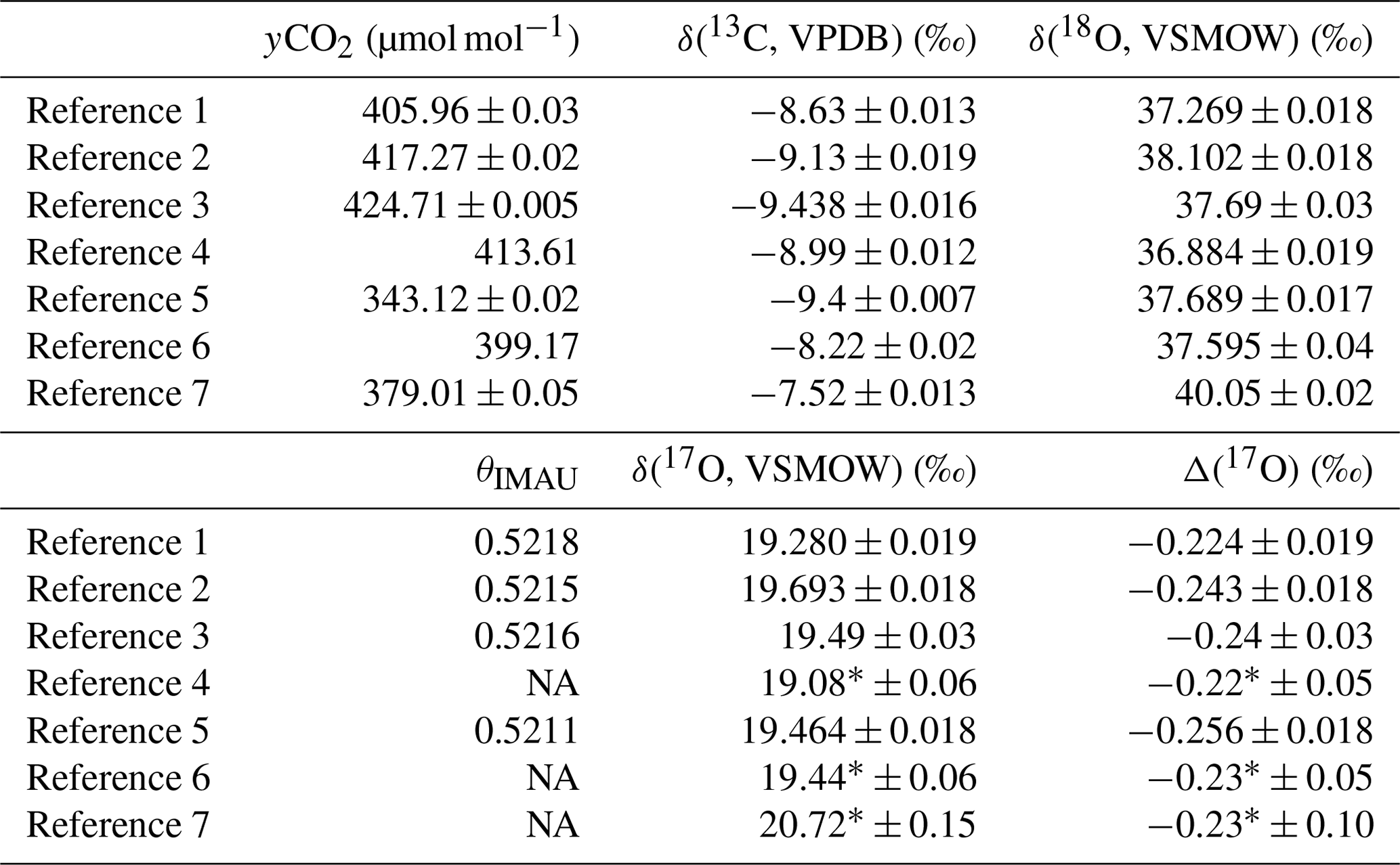
For the calibration of the SICAS isotope measurements, we use the gas references produced in-house, which consist of dried atmospheric air in high-pressure gas cylinders, as presented in Table 1. The CO₂ amount fractions of the references are measured on a Picarro G2401 gas amount fraction analyser and calibrated using in-house working standards linked to the WMO 2019 scale for CO₂, with a suite of four primary standards provided by the Earth System Research Laboratory of the National Oceanic and Atmospheric Administration (NOAA).

To ensure that cylinders with a drifting CO₂ amount fraction are identified, all reference cylinders are measured on the Picarro once a year. The uncertainty of the CO₂ amount fractions in Table 1 is the standard error of those measurements through the years. Considering the low standard errors (between 0.005–0.05 µmol mol⁻¹), there are no signs of drifting CO₂ amount fractions in any of the cylinders. Cylinders 4 and 6 were only measured once, so no standard errors are shown in Table 1.

Aliquots of all references have been analysed at the stable-isotope lab of the Max Planck Institute for Biogeochemistry in Jena (BGC-IsoLab) by dual-inlet IRMS (DI-IRMS) to link the δ(¹³C) and δ(¹⁸O) directly to the JRAS-06 scale (the Jena Reference Air Set for isotope measurements of CO₂ in air (VPDB-CO₂ scale)) (Wendeberg et al., 2013). The stable-isotope compositions of the reference gases measured at BGC-IsoLab and the standard errors of the measurements (standard error of the results of all aliquot measurements) are presented in Table 1.

Despite the existence of this direct linkage of atmospheric CO₂ to the VPDB-CO₂ scale, triple oxygen isotope measurements of atmospheric CO₂ are usually expressed on the VSMOW scale (Hofmann et al., 2017; Adnew et al., 2020; Boering et al., 2004). Also, an internationally recognized isotope scale for δ(¹⁷O) has not been established so far. It is therefore not straightforward to determine the δ(¹⁷O) values of our reference cylinders ourselves. We use the δ(¹⁸O) values measured at BGC-IsoLab in combination with triple oxygen isotope measurements of references 1–3 and 5 conducted at the Institute for Marine and Atmospheric research Utrecht (IMAU) using the O₂–CO₂ exchange method and DI-IRMS measurements (Adnew et al., 2019). The measured θ of the references, calculated as ln(δ(¹⁷O)+1)/ln(δ(¹⁸O)+1) and defined as θ_IMAU from now on, was used to calculate δ(¹⁷O) values on the VSMOW scale from the δ(¹⁸O) values measured by BGC-IsoLab. The latter were converted from VPDB-CO₂ to VSMOW by the following equation, as recommended in Hillaire-Marcel et al. (2021):

$$\begin{array}{}\text{(5)}& {\mathit{\delta }}_{\text{VSMOW}}{(}^{\mathrm{18}}\mathrm{O})=\mathrm{1.04149}\cdot {\mathit{\delta }}_{{\text{VPDB-CO}}_{\mathrm{2}}}{(}^{\mathrm{18}}\mathrm{O})+\mathrm{41.49}\mathrm{‰}.\end{array}$$

Next, the following equation was applied to the BGC-IsoLab δ(¹⁸O)_VSMOW values:

$$\begin{array}{}\text{(6)}& {\mathit{\delta }}_{\text{VSMOW}}{(}^{\mathrm{17}}\mathrm{O})=({\mathit{\delta }}_{\text{VSMOW}}{(}^{\mathrm{18}}\mathrm{O})+\mathrm{1}{)}^{{\mathit{\theta }}_{\text{IMAU}}}-\mathrm{1}.\end{array}$$

Δ(¹⁷O) values were calculated by applying the δ(¹⁸O)_VSMOW and δ(¹⁷O)_VSMOW values to Eq. (3). For the references that were not measured at the IMAU, the δ(¹⁷O) values were determined from SICAS measurements using the calibration methods and uncertainty assignment described before. The Δ(¹⁷O) was subsequently calculated using this measured δ(¹⁷O) and the δ(¹⁸O) measured by BGC-IsoLab. Note that the scale described above for the Δ(¹⁷O) values is indirectly linked to VSMOW, adding uncertainty to the compatibility of other Δ(¹⁷O) scales.

For the measurement of our reference gases by BGC-IsoLab and the IMAU, aliquots were prepared by connecting five sample flasks in series and flushing them with the sample gas, resulting in a similar air sample in all flasks. However, deviations of the sampled air from the air in the reference cylinders as the result of alterations of the gas inside the flasks can be introduced (Steur et al., 2023).

2.4 Comparison of the CIO and IMAU

For a selection of Lutjewad samples, two flasks containing identical air (“duplicate flasks”) were analysed. One of the flasks was measured at the CIO using laser absorption spectroscopy and the other was measured at the IMAU using DI-IRMS to check the compatibility of the two methods. Since 2019, a fully automatic extraction system has been in use at the IMAU, which enables CO₂ to be extracted from air and a sample to be directly analysed using DI-IRMS. Before then, the extraction of CO₂ from the air samples was done at the CIO, and the pure CO₂ samples were sent to the IMAU in flame-sealed tubes for DI-IRMS analysis.

The δ(¹³C) sample differences are higher than expected from the combined uncertainty of the SICAS measurements, as can be seen in Fig. 2. The frequency distribution shows that the differences are at least partly due to systematic errors and possibly scaling or sampling issues. It should be noted that the quality of the SICAS measurements is lower for the samples measured at the end of 2019 and in 2020. Samples from 2018, from which the CO₂ was extracted at the CIO, show a positive offset of the SICAS measurements relative to the IMAU measurements. A reason for the increase in differences in δ(¹³C) values during that period has not been found.

Results for the differences in the δ(¹⁸O) measurements are shown in Appendix A1. The differences are far outside the uncertainty range of the SICAS measurements: they are up to 2 ‰. These high differences are connected to the observations of drift in the oxygen isotopes of CO₂ in flask samples as a function of time (Steur et al., 2023). Δ(¹⁷O) values are not (or are hardly) affected by the drift in oxygen isotopes in the flasks. We calculated that, in the extreme case of a change of more than 3 ‰ in the δ(¹⁸O) of atmospheric CO₂ (Steur, 2023) resulting from the equilibration of CO₂ with water inside the flask and, at the same time, an initial Δ(¹⁷O) value of the CO₂ of −0.69 ‰, the change in Δ(¹⁷O) is less than 0.06 ‰. Considering that the uncertainty of the SICAS Δ(¹⁷O) measurements is always 0.05 ‰ or higher, we can conclude that the effect of the drift of the oxygen isotopes inside the flasks is negligible for the Δ(¹⁷O) values. Results and calculations that support this conclusion can be found in Appendix B1.

In general, the Δ(¹⁷O) differences fall within the mean combined uncertainty of the SICAS measurements over the whole sampling period. The total range of Δ(¹⁷O) of the samples is, however, small: 0.15 ‰. Nevertheless, this comparison shows that the CIO calibration procedure gives Δ(¹⁷O) values similar to those from the IMAU, and the repeatability of the measurements falls within the combined uncertainty of the SICAS measurements. The differences are normally distributed, so there are no systematic offsets between the two labs.

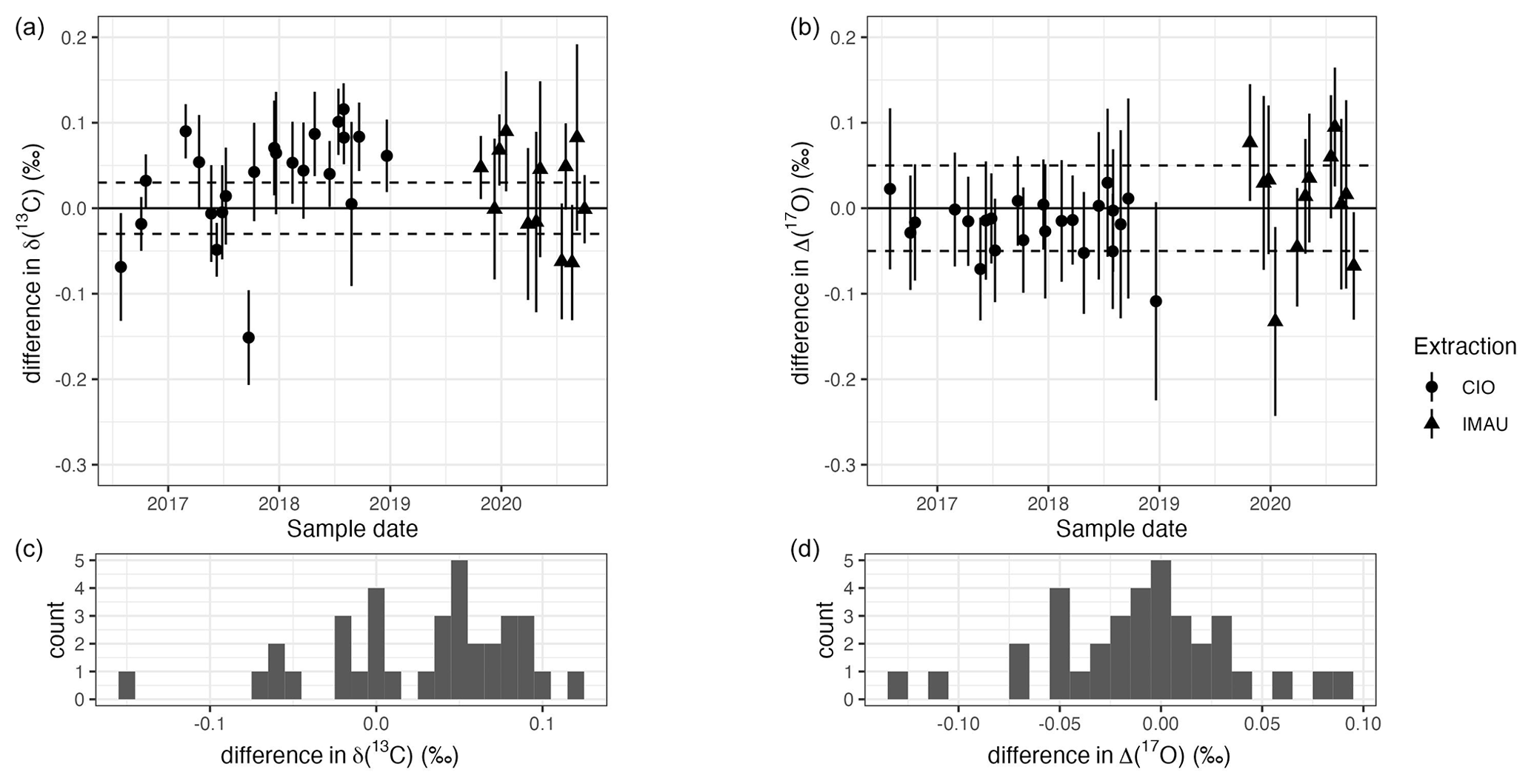
Figure 2 Panels (a) and (b) show the differences (CIO − IMAU) in δ(¹³C) and Δ(¹⁷O) measurements, respectively, between the duplicate flasks. Uncertainty bars show the combined uncertainty (±1σ), as defined in Sect. 2.3, of the CIO measurements. The shape of each data point indicates whether CO₂ was extracted at the CIO and sent to the IMAU as pure CO₂ samples (circles) or the extraction was done at the IMAU (triangles). Panels (c) and (d) show the frequency distributions of the differences.

In Appendix C, we elaborate further on the comparison of Δ(¹⁷O) measurements, and the complete record of Lutjewad Δ(¹⁷O) measurements, including all IMAU measurements, is shown in Fig. C2. This figure shows that the variation that is observed in the IMAU measurements coincides with the variation that is observed in the SICAS measurements.

2.5 Atmospheric modelling of Δ(¹⁷O) in CO₂ at Lutjewad

In addition to the measurements, we present model simulations for Δ(¹⁷O) in CO₂ for the Lutjewad location, which were obtained using the 3-D transport model described in Koren et al. (2019). As the latitudes of Mace Head and Lutjewad are similar, we do not expect to see significant differences between the simulations for the two locations. The model includes the stratospheric input of high Δ(¹⁷O) and processes that will lead to a reduction in the stratospheric signal: biosphere activity, equilibration of CO₂ with soil moisture, CO₂ emissions from fossil-fuel and biomass burning, and CO₂ uptake and emission from the oceans. An update to this model uses meteorological driver data from the ERA5 release (Hersbach et al., 2020) instead of the ERA-Interim fields (Dee et al., 2011) that were used previously. The model resolution applied for the Lutjewad simulation is a longitude–latitude grid of 1° by 1°. Here we present simulations for Δ(¹⁷O) in CO₂ for the years from 2017 until the end of 2021. Note that the long-term mean values simulated by the model for Lutjewad are ultimately dependent on the integrated contribution from all processes across the globe, which are poorly constrained in the model (e.g. due to large uncertainties in soil exchange; see Wingate et al., 2009). Therefore, we focus on the timing and amplitude of the seasonal cycle and the interannual variability of Δ(¹⁷O) in CO₂ at the Lutjewad station.

3 Results and discussion

3.1 CO₂ amount fraction measurement results

In Fig. 3, the CO₂ amount fraction measurements of the Lutjewad and Mace Head flasks measured at the CIO over the period 2017–2022 are shown together with the continuous CO₂ amount fraction measurements from Lutjewad. As an independent comparison, the Mace Head CO₂ amount fraction measurements of discrete air samples from the NOAA Global Monitoring Laboratory Carbon Cycle Greenhouse Gases Cooperative Air Sampling Network (NOAA-GML CCGG) (Lan et al., 2022) are plotted in the same figure. The Mace Head flask samples measured at the CIO are in good agreement (within precision) with the overlapping time series results from the NOAA-GML CCGG. A background CO₂ amount fraction curve has been determined from the Lutjewad continuous CO₂ amount fraction measurements. This was done by including only measurements of samples taken during the daytime (between 10:00 and 19:00 UTC) and excluding hourly averages with standard deviations higher than 0.5 µmol mol⁻¹ and CO values higher than 140 nmol mol⁻¹. Subsequently, the filtered signal was smoothed by a moving average of 30 points and the result was fitted with a quadratic trend with a two-harmonic seasonality. The resulting background signal, shown in Fig. 3 as the black line, corresponds well with the Mace Head measurements. This confirms that the derived background curve represents well-mixed air that is not influenced by local contamination events from fossil fuel burning. This CO₂ amount fraction background curve is used in the stable-isotope records to calculate the Δ^bgy(CO₂) of a sample, which is the difference in amount fraction between the sample and the background curve.

The background curve shows the strong influence of the biosphere, which results in CO₂ amount fractions that are almost 15 µmol mol⁻¹ lower in summer than in winter. The seasonality shows maxima at the beginning of the growing season in March and April and minima at the end of the growing season in August. The overall increase in CO₂ amount fractions in the atmosphere is clearly visible from the background curve and is 2.5 µmol mol⁻¹ a⁻¹. These results are very close to the growth rate of the globally averaged CO₂ amount fractions of 2.4 µmol mol⁻¹ a⁻¹ (standard deviation: 0.5 µmol mol⁻¹ a⁻¹) from 2011 to 2019 (Friedlingstein et al., 2022).

The Lutjewad flasks, although sampled at noon with the aim to sample well-mixed tropospheric air, occasionally show large positive deviations from the background curve, especially in winter; the deviation reached up to +47 µmol mol⁻¹ in December 2017. The CO₂-enriched signals are most probably due to local and regional sources of CO₂, either natural or anthropogenic, that occur on the continent. We therefore expect to see more deviations from the seasonal cycles of stable-isotope values induced by the more continental influence on the Lutjewad record when compared to the Mace Head record.

The Europe-wide drought, which was most severe in northern Europe, during the summer of 2018 (Peters et al., 2020; Ramonet et al., 2020) is clearly visible in the continuous CO₂ amount fraction record of Lutjewad, where a short-term increase in CO₂ amount fractions interrupts the overall decrease in amount fractions that normally occurs over the growing season. In early spring of 2018, CO₂ amount fractions decrease rapidly (when the growing conditions were more favourable; see Smith et al., 2020) until May 2018. Subsequently, a rapid increase in CO₂ amount fractions is observed that lasts until June, before the CO₂ amount fractions start decreasing again. This event is only visible in one Lutjewad flask sample with a Δ^bgy(CO₂) of −8.6 µmol mol⁻¹ and two Mace Head samples from the NOAA-GML CCGG with Δ^bgy(CO₂) values of −6.7 and −7.1 µmol mol⁻¹. Due to the sampling frequency being too low, the drought event is hard to identify from the flask samples only. In 2022, Europe experienced another severe drought, although this was mostly located in central and southeastern Europe (van der Woude et al., 2023). This drought event does not show up in the continuous amount fraction record of Lutjewad, unlike the 2018 drought.

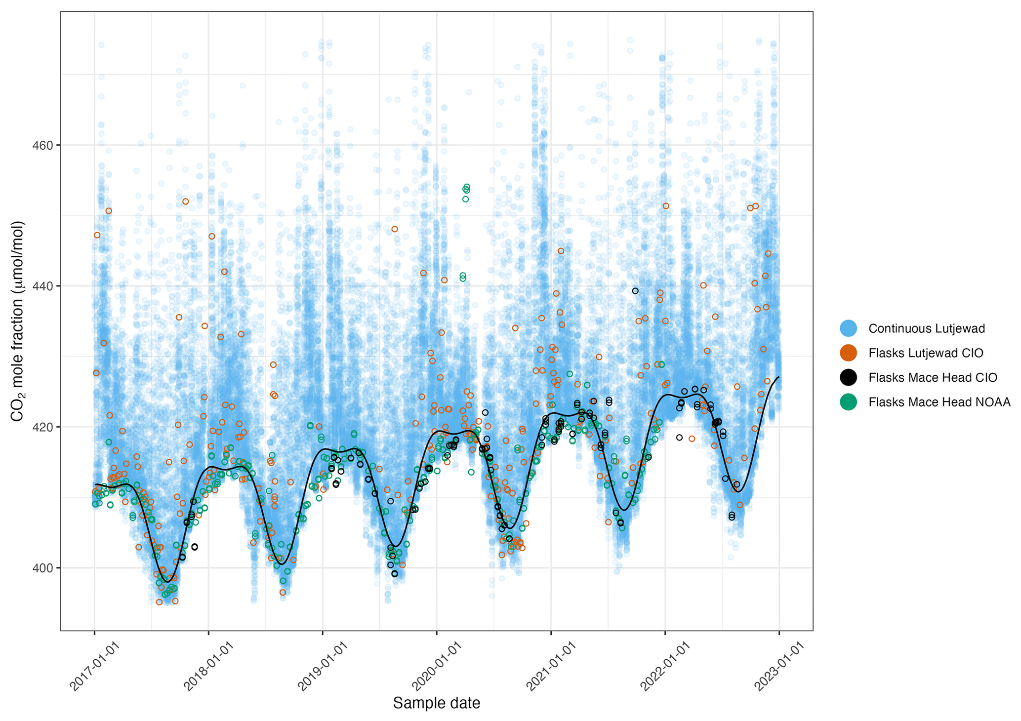
Figure 3 CIO CO₂ amount fractions from continuous measurements (shown as hourly averages) and discrete flask sample measurements from the Lutjewad atmospheric measurement station, and discrete flask sample measurements from the Mace Head atmospheric measurement station from the NOAA-GML Carbon Cycle Cooperative Sampling Network and the CIO. The seasonal cycle (black line) is derived from the filtered continuous measurements, which were fitted with a quadratic trend with a two-harmonic seasonality.

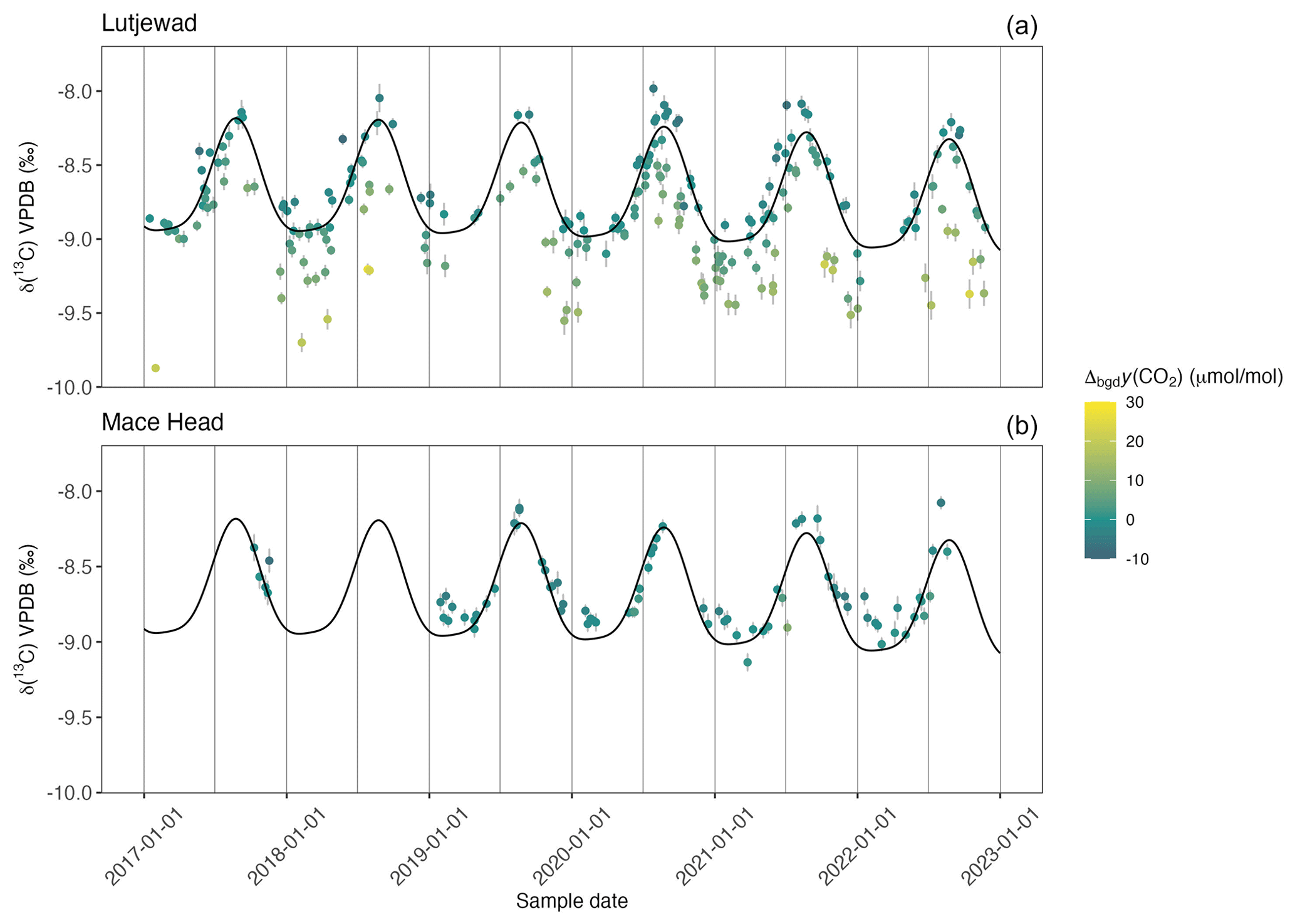
Figure 4 δ(¹³C) records of Lutjewad and Mace Head from SICAS flask measurements of atmospheric CO₂. Panel (a) shows δ(¹³C) measurements from Lutjewad, and (b) shows those from Mace Head. The combined uncertainty of the measurements is shown as grey error bars (±1σ) and include the measurement uncertainty, repeatability, accuracy and uncertainty introduced as a consequence of the calibration method used. Δ^bgy(CO₂) is indicated by the colour of the data point. The seasonality curve was derived by fitting the Lutjewad δ(¹³C) values of samples that had Δ^bgy(CO₂) values that were no higher than 5 µmol mol⁻¹ and is shown as the black line in both graphs (the Lutjewad seasonal curve is also shown in the Mace Head graph). The fitting method that was used is the same as that used for the CO₂ background curve.

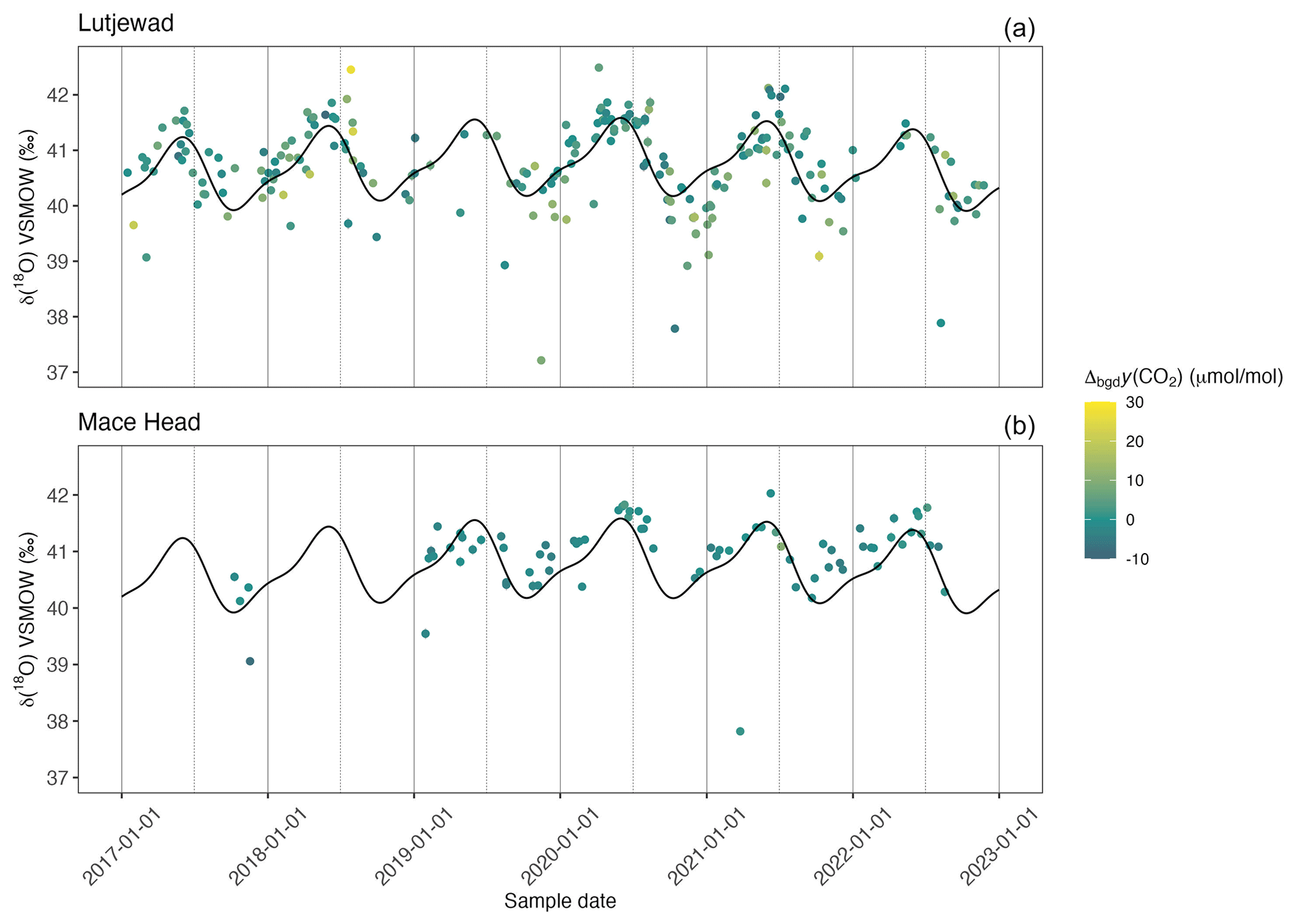
Figure 5 δ(¹⁸O) records from Lutjewad (a) and Mace Head (b) from SICAS flask measurements of atmospheric CO₂. The combined uncertainties are shown as grey error bars (±1σ) and include the measurement uncertainty, repeatability, accuracy and uncertainty introduced as a consequence of the calibration method used. Δ^bgy(CO₂) is indicated by the colour of the data point. The seasonality curve was derived by fitting the Lutjewad δ(¹⁸O) values of samples that had Δ^bgy(CO₂) values that were no higher than 5 µmol mol⁻¹ and is shown as the black line in both graphs (the Lutjewad seasonal curve is also shown in the Mace Head graph). The fitting method that was used is the same as that used for the CO₂ background curve.

3.2 Stable-isotope measurements

Results of δ(¹³C) measurements of atmospheric CO₂ in discrete flask samples from Lutjewad and Mace Head are shown as a function of sampling date in Fig. 4. A quadratic trend with a two-harmonic seasonality was fitted to all Lutjewad δ(¹³C) points that had a Δ^bgy(CO₂) value that was no higher than 5 µmol mol⁻¹. There are too few data points to obtain a fit to the Mace Head record. Instead, the Lutjewad seasonal trend is also plotted onto the Mace Head record so that both records can be easily compared. The seasonality in the δ(¹³C) records shows a strong anti-correlation with the CO₂ amount fraction records, with maxima occurring during late summer and minima during late winter. During winter, there are negative excursions in the Lutjewad record that do not appear in the Mace Head record, from which we can conclude that the Lutjewad δ(¹³C) is influenced more by local or regional signals, resulting in more-depleted δ(¹³C) signals like those due to fossil fuel burning emissions and plant and soil respiration (Keeling et al., 2017; Scholze et al., 2008). For the same reason, the seasonal curve derived from the Lutjewad data shows a stronger decrease in δ(¹³C) values in autumn and winter than seen in the Mace Head record. While Lutjewad would be more influenced by the strong biosphere activity on the continent, heavier (i.e. less negative) δ(¹³C) values than at Mace Head would be expected during the summer. This is the case for the years 2020 and 2021, but the Mace Head values are heavier for 2019. The year 2019 was, however, a period in which Lutjewad samples were collected more sparsely due to problems with the sampling system. It is therefore hard to conclude whether there is, in general, a heavier δ(¹³C) signal at Lutjewad compared to Mace Head during summers. Overall, a decreasing trend is observed from the seasonal fit, which is explained by increased CO₂ amount fractions in the atmosphere due to the combustion of fossil fuels, also known as the ¹³C Suess effect (Keeling, 1997).

Measurements of δ(¹⁸O) of atmospheric CO₂ from Lutjewad and Mace Head flask measurements conducted at the SICAS are presented in Fig. 5. A seasonal curve was fitted to the Lutjewad data using the same method as used for the δ(¹³C) data. The Mace Head observations coincide with the Lutjewad fit, with maxima occurring in May and June and minima in December and January. Although the maximum and minimum values are very similar, the maximum values in Mace Head during the summer of 2022 are more enriched than the Lutjewad values. These differences might be explained by the difference in δ(¹⁸O) composition between the source waters for the vegetation at both sites (Levin et al., 2002). It should be noted that many of the δ(¹⁸O) values of the atmospheric CO₂ samples shown here are likely to have a bias towards depletion due to the drift we observe over time, as explained in Sect. 2.4. Any interpretation of the absolute changes in the δ(¹⁸O) values should therefore be done with caution, taking the storage time into account.

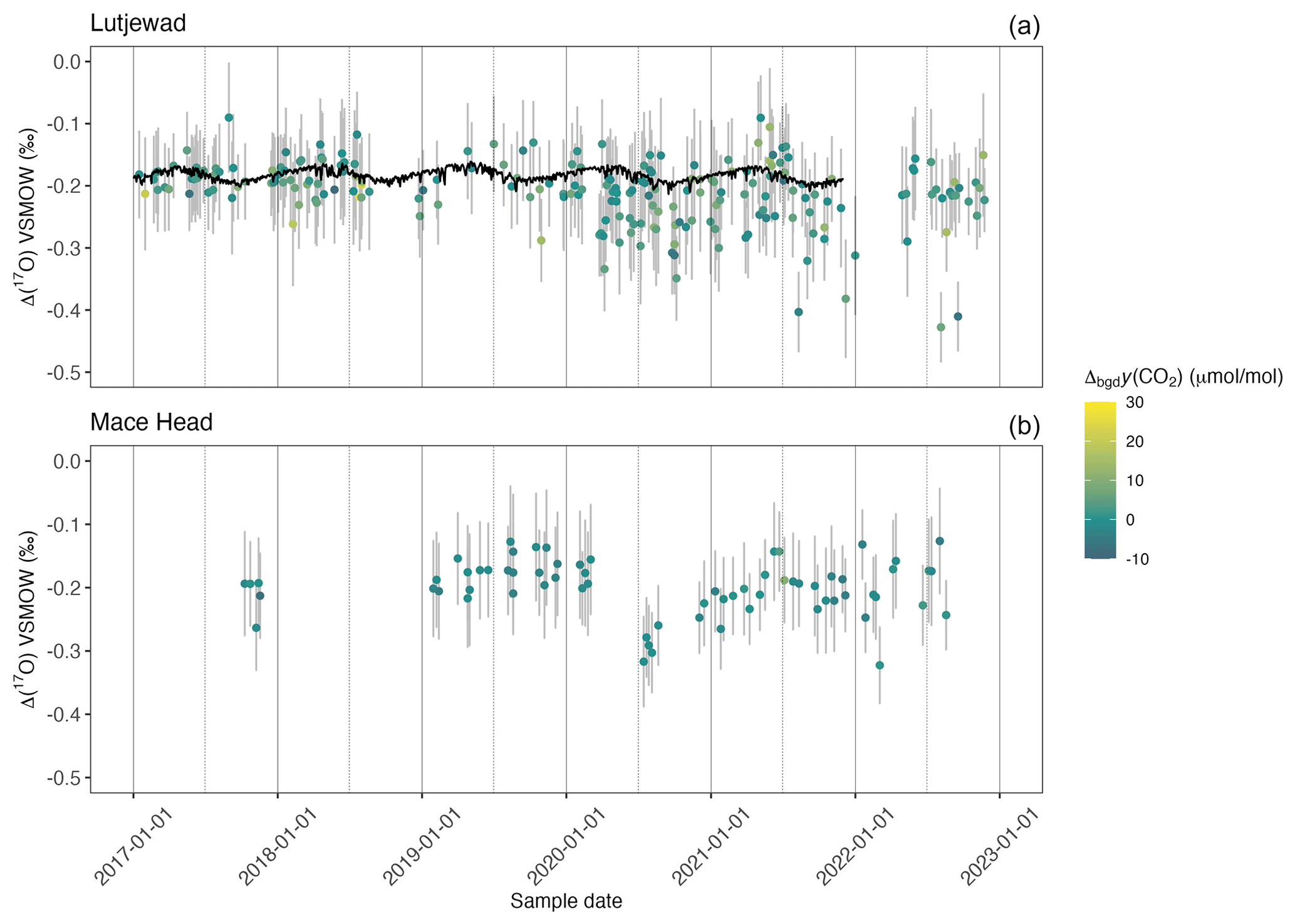
Figure 6 Δ(¹⁷O) records from Lutjewad (a) and Mace Head (b) from SICAS flask measurements of atmospheric CO₂. The combined uncertainties are shown as grey error bars (±1σ) and include the measurement uncertainty, repeatability, accuracy and uncertainty introduced as a consequence of the calibration method used. Δ^bgy(CO₂) is indicated by the colour of the data point. Model simulations of values obtained daily at 13:00 UTC at Lutjewad (Koren et al., 2019) are shown in the upper graph as the black line.

Δ(¹⁷O) measurements from the Lutjewad and Mace Head stations are presented in Fig. 6. The total ranges in the Lutjewad and the Mace Head records are 0.5 ‰ and 0.2 ‰, respectively, with an average combined uncertainty of the measurements of 0.07 ‰ for both records. Following Koren et al. (2019), we would expect to see a seasonality of increasing Δ(¹⁷O) values over winter and decreasing values over summer, when the biosphere is most active. We plotted Δ(¹⁷O) against 1 $/$ (CO₂ amount fraction) and δ(¹³C) for summer and winter values of Lutjewad (see Fig. D1 in the Appendix). Mace Head was excluded from this analysis as the many data gaps over the measurement period led to an unrepresentative result. If seasonality resulting from the biosphere activity is present, this should show up in the plots as a distinction between Δ(¹⁷O) summer and winter values. Also, correlations between the Δ(¹⁷O) and the 1 $/$ CO₂ and δ(¹³C) would be expected, as the latter two also follow this seasonality. We did not observe any of this, indicating that there is no significant seasonality caused by the biosphere signal in our Lutjewad Δ(¹⁷O) record. This differs from results for the Göttingen record over the period 2010–2012, where a seasonality was observed, with maximum values occurring during June and July (Hofmann et al., 2017). The amplitude of the seasonality that was determined from the Göttingen Δ(¹⁷O) record is (0.13±0.02) ‰. If such a seasonality was present in the Lutjewad and Mace Head records, we would expect to see it, as this signal is higher than the average combined uncertainty of the SICAS measurements. It could be that, due to its more continental location, the amplitude of the Δ(¹⁷O) seasonality is higher at the Göttingen site, reflecting a stronger biosphere signal. A model simulation of the Göttingen location shows an amplitude of 0.045 ‰ (Hofmann et al., 2017), while the amplitude of the simulation for the Lutjewad location, shown as the black line in Fig. 6, is close to 0.025 ‰. The model used in Hofmann et al. (2017) is an earlier version of the model used in this study (Koren et al., 2019), so the results should be strongly comparable. The higher amplitude for the simulation for the Göttingen location confirms the hypothesis of a higher Δ(¹⁷O) seasonality due to its more continental location in comparison with Lutjewad. It is unlikely that a considerably lower seasonal signal than observed at the Göttingen location would be detected by the SICAS measurements, considering their average combined uncertainties.

The low sampling frequency in combination with the sampling method used at both locations will complicate the capture of small seasonal variations. Air samples represent only a snapshot in time, while, at the same time, the frequency of sampling is only once every 3 d (Lutjewad) or even once every week (Mace Head) (Nevison et al., 2011). Changing the sampling method to a method in which the sampled air evenly represents a certain sampling period would decrease the influence of short-term variability in the atmospheric composition at the sampling site (Chen et al., 2012). To get a much higher sampling frequency for Δ(¹⁷O) measurements at Lutjewad in the future, our laser absorption spectroscopy system will be deployed in the (semi-)continuous measurement mode, a technique already shown by Kaiser et al. (2022). This will enable us to apply rigid filtering of the data to derive either results representative of well-mixed background air or, on the other hand, results that are representative of air masses from the continent.

The most important difference between the Lutjewad and Mace Head Δ(¹⁷O) records is the presence of more-depleted values in the Lutjewad record, with the lowest value being −0.43 ‰ in the summer of 2022. CO₂ equilibrated with water with λ_RL will have an Δ(¹⁷O) of −0.21 ‰. In summer, leaf water gets enriched in oxygen isotopes and depleted in Δ(¹⁷O) as the result of high rates of evapotranspiration (Landais et al., 2006). Due to the active biosphere during summer, CO₂ and leaf water will equilibrate, and the depleted Δ(¹⁷O) signal will be translated to the CO₂ (Adnew et al., 2023). We estimated that this could result in Δ(¹⁷O) values being up to 0.1 ‰ more depleted when assuming the minimum θ of 0.516 for evapotranspiration (Landais et al., 2006) and considering the range of δ(¹⁸O) values that were measured in our Lutjewad record. For the full estimation, we refer the reader to Appendix E. Δ(¹⁷O) values down to −0.31 ‰ can be explained by this process. CO₂ emitted from combustion processes has very negative Δ(¹⁷O) values (Laskar et al., 2016; Horváth et al., 2012). All points that have lower Δ(¹⁷O) values than −0.3 ‰ and are sampled during winter/spring have more-depleted δ(¹³C) values and more-enriched CO₂ values than would be expected from the seasonal trends. This indicates that local CO₂ emission sources are the reason for the more-depleted Δ(¹⁷O) values in winter. Samples that are very enriched in CO₂ amount fractions are not shown here, as these results have very high measurement uncertainties. This could be the reason that a correlation of Δ(¹⁷O) and CO₂ amount fractions does not appear in Fig. D1. A few points show depletions lower than −0.31 ‰ without CO₂ amount fraction enrichments, and these currently remain unexplained.

Significant differences in Δ(¹⁷O) values over time are observed in both records. In the Lutjewad record, we observe Δ(¹⁷O) values that are above or close to −0.2 ‰ at the beginning of 2020. Then the values decrease until they reach minimum values in October 2020, with the lowest value in that period being −0.34 ‰. An increase in Δ(¹⁷O) values is observed after this period, and May 2021 is a period with more-elevated values, with the highest observation being −0.09 ‰. Although the Mace Head record shows gaps over the period from 2020–2021, it is clear that values at the beginning of 2020 are higher than those at the end of 2020. This interannual variability in both records indicates that processes other than biosphere activity cause most of the variation at the measurement locations.

3.3 Sensitivity analysis of the simulated Δ(¹⁷O) interannual variability

The total variation predicted by a local simulation of the model (base version in Koren et al., 2019) for the location of Lutjewad is lower than the uncertainty and variability of the SICAS measurements and has seasonal character only. The model simulation of Δ(¹⁷O) of atmospheric CO₂ is shown for the Lutjewad mid-latitude band as the black line in Fig. 6. Daily values at 13:00 UTC (corresponding to 14:00 or 15:00 local time) are shown. These represent well-mixed afternoon conditions, which are typically more reliable in relatively coarse global models than simulated nighttime or early-morning values. Although small, there is a clear seasonality, with the highest Δ(¹⁷O) values occurring in early spring, when the stratospheric influx is highest, with low biospheric activity aggregated over the preceding months, and with the lowest values occurring during early autumn, when the biospheric carbon uptake has depleted the tropospheric Δ(¹⁷O) budget. The values are all between −0.16 ‰ and −0.21 ‰, which is significantly narrower than the observed range at Lutjewad. It is therefore clear that the current model version does not capture the variation in Δ(¹⁷O) that is measured in the Lutjewad record. The Göttingen record (Hofmann et al., 2017) also shows significant interannual changes in Δ(¹⁷O) values of 0.1 ‰, which have not been explained so far. In that record spanning the period from June 2010 until August 2012, they found a negative shift in the Δ(¹⁷O) values from the summer of 2011 until the end of the record.

The biosphere sink of Δ(¹⁷O) cannot have caused the interannual changes in the records since a stronger or weaker seasonal cycle would then also be expected to occur. The variations observed in the Lutjewad and Mace Head records are furthermore driven by anomalies in multiple seasons and are not limited to summer or winter periods only. Besides the biospheric sink, the other main term in the Δ(¹⁷O) budget is its stratospheric production and downward transport. We therefore hypothesize that the stratospheric input of Δ(¹⁷O) is not well parameterized in the model, leading to the limited interannual variability that is simulated in Fig. 6.

In the 3-D atmospheric model, the stratospheric production of Δ(¹⁷O) of atmospheric CO₂ is implemented using its empirical relation with the stratospheric N₂O amount fraction (see Sect. 2.2 in Koren et al., 2019, for a more detailed description), as shown in the equation below:

$$\begin{array}{}\text{(7)}& {\mathrm{\Delta }}_{\mathrm{fit}}{(}^{\mathrm{17}}\mathrm{O})=a(y_{\mathrm{dtd}}\left({\mathrm{N}}_{\mathrm{2}}\mathrm{O}\right)-\mathrm{320.84}\mathrm{nmol}{\mathrm{mol}}^{-\mathrm{1}})+b,\end{array}$$

where Δ_fit(¹⁷O) is the assigned stratospheric signature, [N₂O]_dtd is the detrended N₂O amount fraction, and a and b are empirical fit coefficients. The N₂O amount fraction in the stratosphere and the Δ(¹⁷O) in CO₂ are negatively correlated based on measurements from four different studies, as presented in Koren et al. (2019). The use of this relation as the only driver for the Δ(¹⁷O) source from the stratosphere is very coarse, and it is possible that factors such as temperature, as postulated by Wiegel et al. (2013), have an effect on the Δ(¹⁷O) enrichment of CO₂ in the stratosphere.

To increase variability in the simulated stratospheric production of Δ(¹⁷O), we included an additional empirical production term for the region from 60–90° N in winter based on 100 hPa temperature anomalies (over this same period and region) from the National Centers for Environmental Prediction (NCEP). The temperature at 100 hPa at 60–90° N or the lower-stratosphere temperature is shown to be a proxy for stratosphere–troposphere exchange during the months of January to March, as it is linked to the strength of the polar vortex, which negatively correlates with the strength of the Brewer–Dobson circulation (Newman et al., 2001; Nevison et al., 2007). The Brewer–Dobson circulation is the meridional circulation that is driven by large-scale temperature gradients on the earth and leads to ascending air near the tropics and the subsidence of air near the poles. A strong Brewer–Dobson circulation will lead to the intrusion of higher volumes of stratospheric air into the troposphere during winter, when the polar vortex is weaker (Nevison et al., 2007). This links the lower stratosphere temperature during the Northern Hemisphere winter to the strength of the input of CO₂ with a high Δ(¹⁷O) composition into the troposphere. The adjusted Δ(¹⁷O) production term is defined as

$$\begin{array}{}\text{(8)}& \begin{array}{rl}{\mathrm{\Delta }}_{\mathrm{source}}{(}^{\mathrm{17}}\mathrm{O})& =\stackrel{\mathrm{original}\mathrm{production}\mathrm{term}}{\overbrace{a\left(y_{\mathrm{dtd}}\right({\mathrm{N}}_{\mathrm{2}}\mathrm{O})-\mathrm{320.84}\mathrm{nmol}{\mathrm{mol}}^{-\mathrm{1}})+b}}\\ & +\stackrel{\mathrm{added}\mathrm{term}}{\overbrace{c\mathrm{\Delta }{T}_{\mathrm{100}\mathrm{hPa}}}},\end{array}\end{array}$$

where the first part is repeated from Eq. (7) and the last term, which has been added, describes the imposed coupling with temperature anomalies at the 100 hPa level ΔT^100 hPa, with c being a tunable parameter. Here, the empirical parameters a, b and c are constant for a given simulation, whereas the [N₂O]_dtd value differs for each grid point and with time. The temperature anomaly ΔT^100 hPa is determined by taking the average temperature of the months January, February and March at 100 hPa for 60–90° N per year for the period 2017–2022. Subsequently, the difference between these values and the average for all 6 years is calculated. In Eq. (7), it is set to zero for regions below 60° N and for the months April–December. Note that both the N₂O amount fractions and the temperature anomaly are used as proxy values for the Δ(¹⁷O) value in the stratosphere. Thereby, the temperature relation represents both the temperature dependence of the actual Δ(¹⁷O), as suggested in Wiegel et al. (2013), and the temperature dependence of stratospheric exchange, which might not be sufficiently represented with only 25 vertical layers, as used in the current model (see e.g. Bândă et al., 2015, for the influence of vertical resolution on stratosphere–troposphere exchange).

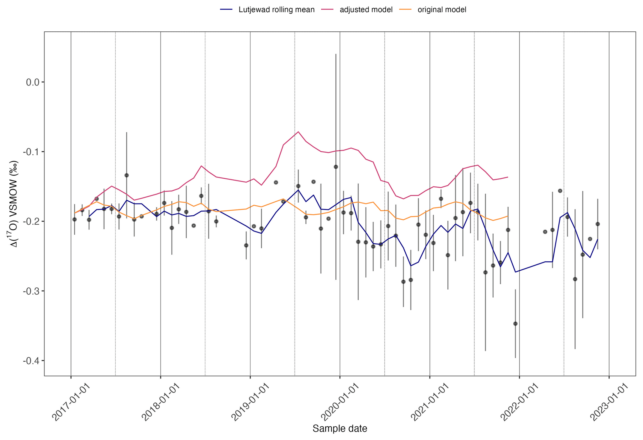
Figure 7 The black dots show the monthly averages of the Lutjewad Δ(¹⁷O) record, while each error bar shows the standard deviation (±1σ) of all the values per month. The plotted lines show the Lutjewad rolling mean (window =3), the original model simulation (as described in Koren et al., 2019) and the monthly averages of the adjusted model simulation in which the input of Δ(¹⁷O) into the troposphere is linked to the lower-stratosphere temperature.

The simulation with the adjusted Δ(¹⁷O) production term is in much better agreement than the original Lutjewad simulation, as can be seen in Fig. 7. It is striking that over the years 2019–2021, the model simulation follows the running average of the measurements very well, with a correlation coefficient of 0.82 for this period. For the years 2017 and 2018, the data and the model agree in that there is much less interannual variability in both the measurements and the model simulation. However, the comparison of small-scale variability is hampered by the relatively high uncertainty of the measurements. The overall variability over the full record is −0.19 ‰ to −0.07 ‰ for the model simulation and −0.27 ‰ to −0.16 ‰ for the moving average of the measurements. Although the absolute values of the measurements and the model differ by 0.08 ‰, the overall variability of the simulation with the adjusted Δ(¹⁷O) production term increased significantly and is close to the overall variability of the measurements. The much-improved agreement of the model simulation and the measured Δ(¹⁷O) indicates the need to revise the stratospheric source of the model, which is now done using the empirical relation with stratospheric N₂O amount fractions. This will lead to a more realistic input of high Δ(¹⁷O-CO₂) into the troposphere.

The added source production term linked to the lower-stratosphere temperature is chosen for the adjusted-model simulation because of its connection to troposphere–stratosphere transport at higher latitudes as well as its relation to ozone concentrations in the stratosphere. A weak polar vortex is accompanied by elevated stratospheric temperatures and more stratosphere-to-troposphere downwelling, while low stratosphere temperatures lead to a more stable polar vortex and therefore less downward transport (Newman et al., 2001; Kidston et al., 2015). On top of that, we should consider the role of ozone amount fractions in the stratosphere in the formation of CO₂ with high Δ(¹⁷O) values. The formation of polar stratospheric clouds that accelerate the destruction of ozone is known to occur during anomalous cold conditions when the polar vortex is strong and stable (Lawrence et al., 2020). We hypothesize that colder lower-stratosphere temperatures at 60–90° N lead to enhanced ozone destruction in the polar vortex, which might in return reduce the production of high Δ(¹⁷O-CO₂) in the stratosphere during late winter and early spring in the Northern Hemisphere (given the role of ozone in the production of Δ(¹⁷O) stratospheric CO₂; Yung et al., 1991). This will result in generally lower Δ(¹⁷O) values for tropospheric CO₂ after that period. This ozone-dependent process would then be the atmospheric transport process that reduces the Δ(¹⁷O) budget in the troposphere. The considerations above indicate that, especially in more anomalous stratospheric conditions at both higher- and lower-than-average temperatures, the stratospheric Δ(¹⁷O) source is likely to deviate from the linear fit of stratospheric N₂O amount fractions to Δ(¹⁷O) values in CO₂, as used in Koren et al. (2019). We acknowledge that our empirical modification still does not accurately describe the intricate complexities of the stratospheric production of Δ(¹⁷O), but it does at least allow us to assess the relevance of the stratospheric source to the model simulation, and it shows the direction in which further model improvements can be beneficial.

Summarizing, we do observe interannual changes in both the Lutjewad and Mace Head records, possibly caused by variations in the stratospheric source of enriched Δ(¹⁷O). No seasonal cycle, which would be an expected effect of the biosphere, is observed, but stratosphere–troposphere exchange seems to cause the highest variations in Δ(¹⁷O).

4 Conclusion and outlook

In this study, we showed that Δ(¹⁷O) measurements for atmospheric CO₂, as well as δ(¹³C) and δ(¹⁸O) measurements, can be performed using laser absorption spectroscopy, thereby drastically reducing the sample preparation time in comparison with IRMS measurements. This opens up the opportunity to do long-term monitoring studies or field studies more easily, and it could lead to an increase in Δ(¹⁷O) measurements for atmospheric CO₂ in the near future. With our analysis method, we reach combined uncertainties of 0.05 ‰ when the sample CO₂ amount fraction is within the range of the reference gases and the sample does not differ by more than 15 µmol mol⁻¹ from the nearest reference. Extrapolation of the calibration curves or a large difference between the sample and the nearest reference introduces uncertainty into the results, showing the importance of including enough reference gases in the calibration. For δ(¹³C) and δ(¹⁸O) measurements, we reach combined uncertainties of 0.03 ‰ and 0.05 ‰, respectively, under good calibration conditions. Seasonal cycles as well as long-term trends, as can be expected from the known sources and sinks of ¹³C and ¹⁸O, were clearly identified in the Lutjewad and Mace Head measurement records. The Δ(¹⁷O) records show significant interannual variability at both measurement locations. A seasonal cycle is not observed, possibly because the uncertainties of the measurement results were too high. The measurement instrument will be used for semi-continuous measurements at the Lutjewad station in the near future. This will result in a much higher sampling frequency, so rigorous filtering can be applied to the measurement results. In this way, we hope to link variations in the records to specific events, which will help us understand the Δ(¹⁷O) budget of atmospheric CO₂ in the troposphere better.

As original-model simulations do not capture the interannual variability observed in the measurements, we revised the model's definition of the stratospheric input of CO₂ with a high Δ(¹⁷O) value into the troposphere by linking it to temperature anomalies of the lowermost stratosphere at 60–90° N as a proxy for the downwelling strength. This resulted in much stronger interannual variability in the model simulation for the Lutjewad location, which closely followed the variations in Δ(¹⁷O) measurements for the years 2019–2021. This suggests that the interannual variability in the tropospheric budget of Δ(¹⁷O) as observed in the Lutjewad measurements is more strongly coupled to year-to-year variations in the stratospheric downwelling of enhanced Δ(¹⁷O) values in CO₂ than previously assumed.

Appendix A: δ(¹⁸O) differences between SICAS and IMAU flask measurements

δ(¹⁸O) measurements of samples that should be identical were conducted at the IMAU and with the SICAS and were found to differ strongly, as can be seen in Fig. A1. We argue that this is due to the drift of the oxygen isotopes in the flasks, a phenomenon described in (Steur et al., 2023). In Fig. A2, the difference in δ(¹⁸O) (SICAS − IMAU) is plotted against the difference in storage time for the flasks for which the date of CO₂ extraction is known. The samples for which the CO₂ was extracted at the IMAU show a negative trend, as expected from the fact that, over time, δ(¹⁸O) values drift towards more-negative values. The samples extracted at the CIO do not show this trend, possibly due to the fact that another extraction method was used, adding more uncertainty to the δ(¹⁸O) values. The time that passed before samples were measured at the IMAU after extraction at the CIO is very variable. It is possible that the pure CO₂ samples drifted over time. This extra uncertainty factor is not included in this analysis.

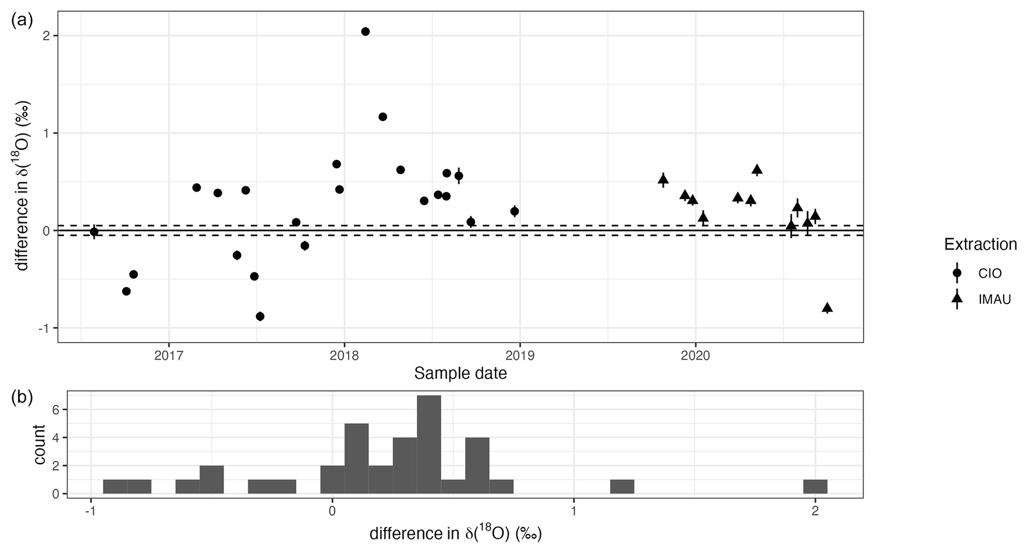
Figure A1 Panel (a) shows the differences (CIO − IMAU) between the δ(¹⁸O) measurements for the duplicate flasks. The uncertainty bars show the combined uncertainty of the CIO measurements. The shape of the data point indicates whether the CO₂ was extracted at the CIO and sent to the IMAU as a pure CO₂ sample (circles) or the extraction was done at the IMAU (triangles). Panel (b) shows the frequency distribution of the differences.

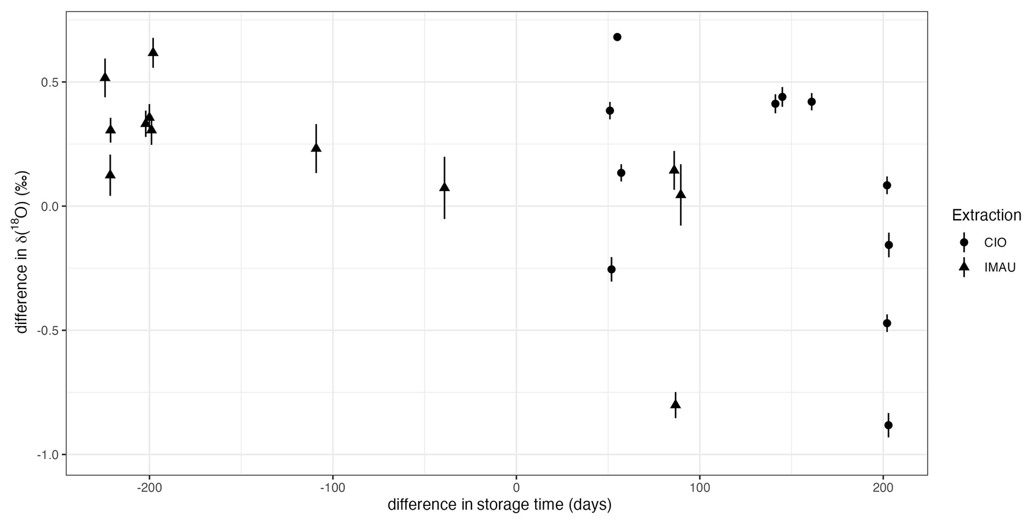
Figure A2 The difference between the δ(¹⁸O) measurements for the duplicate flasks (CIO − IMAU) is plotted against the difference in storage time (CIO − IMAU). The uncertainty bars show the combined uncertainty (±1σ) of the CIO measurements. The shape of each data point indicates whether the sample was extracted at the CIO (circles) or at the IMAU (triangles).

Appendix B: Sensitivity analysis of the drift of Δ(¹⁷O) in glass sample flasks

To determine the change in Δ(¹⁷O) as the result of the drift of the oxygen isotopes of atmospheric CO₂ inside glass sample flasks (Steur et al., 2023), a simulation of the various changes was conducted. In an earlier study, we showed that small amounts of water inside the flasks will change the original oxygen isotope composition of the atmospheric CO₂ as the CO₂ and water will equilibrate. Water builds up inside the flasks over time through sampling and through the permeation of water into the flask through the Viton O-rings (Steur et al., 2023). For the simulation, we use 2.3 L flasks containing air with a CO₂ amount fraction of 400 µmol mol⁻¹ at atmospheric pressure. The initial δ(¹⁸O) of the atmospheric CO₂ is 37 ‰ on the VSMOW scale – within the atmospheric range. The δ(¹⁷O) varies such that there are simulations for initial Δ(¹⁷O) values of 0.31 ‰, −0.09 ‰, −0.19 ‰, −0.29 ‰ and −0.69 ‰. These values were chosen as they correspond to variations around the water–CO₂ equilibration line with a λ of 0.5229 (Barkan and Luz, 2012). For the initial δ(¹⁸O) and δ(¹⁷O) of the water, we use −12.91 ‰ and −6.77 ‰ VSMOW, respectively. The Δ'(¹⁷O) value of the water is 0.07 ‰. These values are measurement results for water extracted from lab air, which was measured with an LGR OA-ICOS liquid water isotope analyser. We assume that all the CO₂ and water equilibrate over time. The amount of water inside the flask varies between 10⁻⁴ and 10⁻⁶ g such that equilibration causes changes in the δ(¹⁸O) of the atmospheric CO₂ of between −3.27 ‰ and −0.03 ‰. It should be noted that changes of more than 3 ‰ in δ(¹⁸O) are very high, as changes of 0.48 ‰ were observed after 114 d of storage in similar conditions, as described above (Steur et al., 2023). The change in the Δ(¹⁷O) of the atmospheric CO₂ ranges between −0.005 ‰ and 0.06 ‰ for all scenarios described above and is limited to −0.002 ‰ and 0.01 ‰ for a realistic maximum drift of −0.48 ‰ (see also Fig. B1).

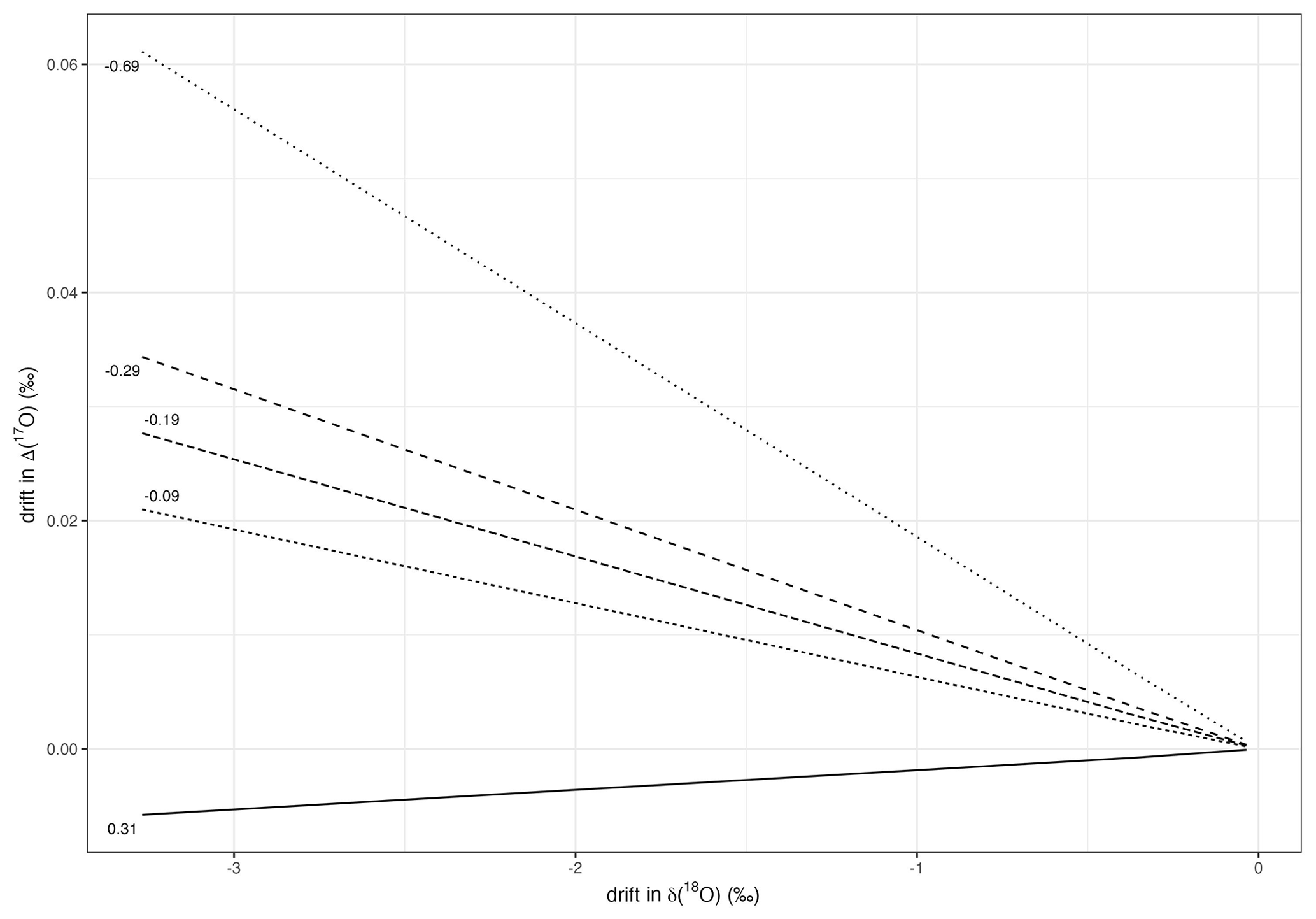
Figure B1 Results of a sensitivity analysis of the drift of the Δ(¹⁷O) of atmospheric CO₂ in a 2.3 L glass sample flask as a function of the drift in δ(¹⁸O). The initial Δ(¹⁷O) value of the atmospheric CO₂ is indicated per line.

Appendix C: Lutjewad Δ(¹⁷O) measurements from the CIO and IMAU compared

Two identical flask samples (duplicates) have occasionally been taken at Lutjewad with the aim of comparing measurements from the SICAS with IRMS measurements from the IMAU. For Δ(¹⁷O) measurements, this comparison is hard to make, considering the very low variance that is observed in the duplicate samples from the Lutjewad station. Also, not all the duplicates have been measured by both labs. Figure C1 shows the results for identical samples measured at the IMAU and CIO in a space representative of the total range of Δ(¹⁷O) that was measured at Lutjewad. From the figure, it is clear that the identical samples that were measured do not represent the full range of Δ(¹⁷O): from −0.4 ‰ to −0.1 ‰. We should also consider the (undefined) uncertainty added by the extraction of the CO₂ from air, which is done for the IMAU measurements but not for the SICAS measurements.

When considering, however, all data points for the Lutjewad flasks from the SICAS and from the IMAU, significant interannual variability is reflected in both datasets. Both the IMAU and the SICAS measurements show lower values in 2020 than in the period before, as observed in Fig. C2.

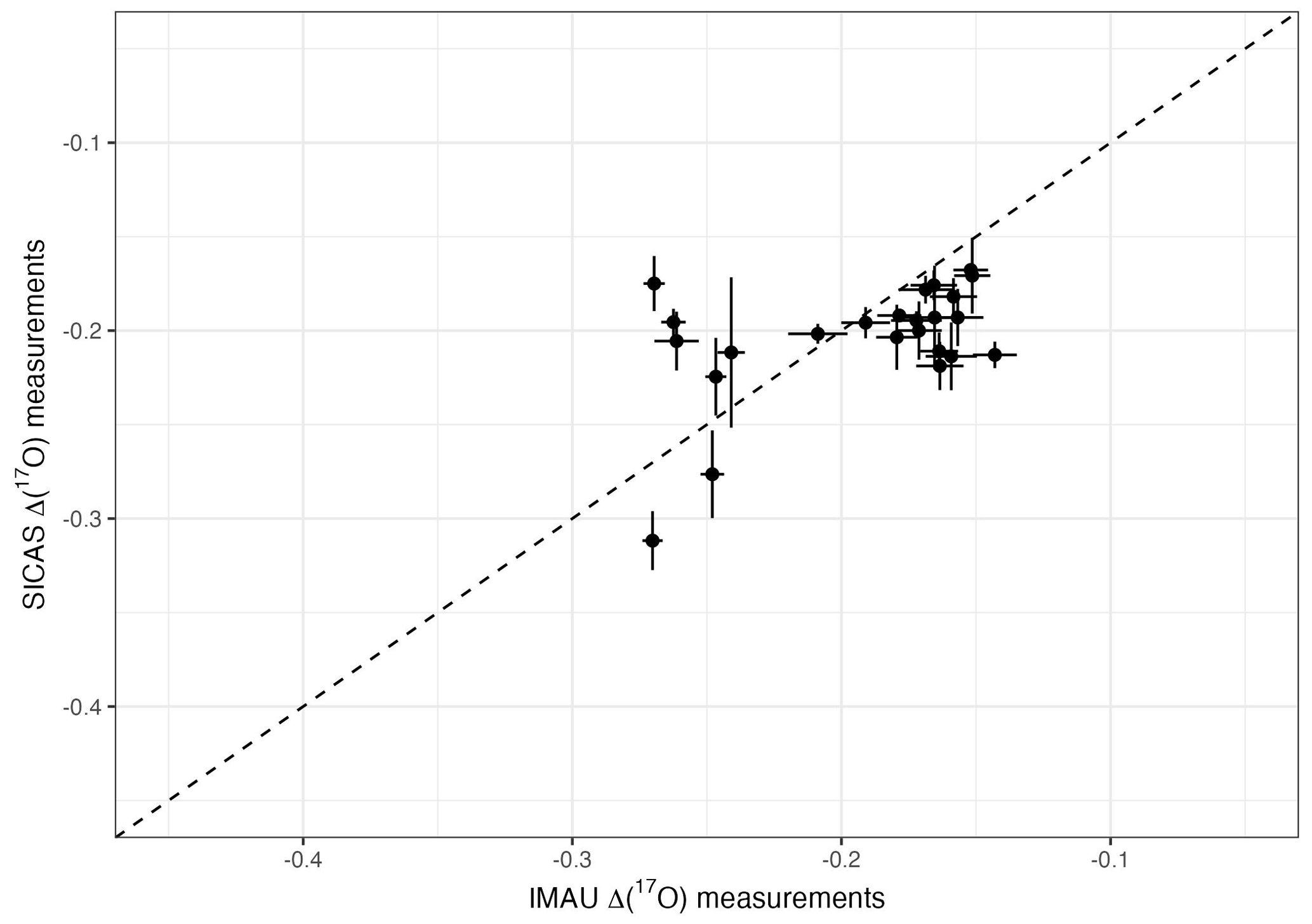
Figure C1 Δ(¹⁷O) measurements conducted with IRMS at the IMAU (x axis) and conducted with the SICAS (y axis), all in ‰. The error bars show the standard errors of the measurements. The dashed line is the 1:1 ratio.

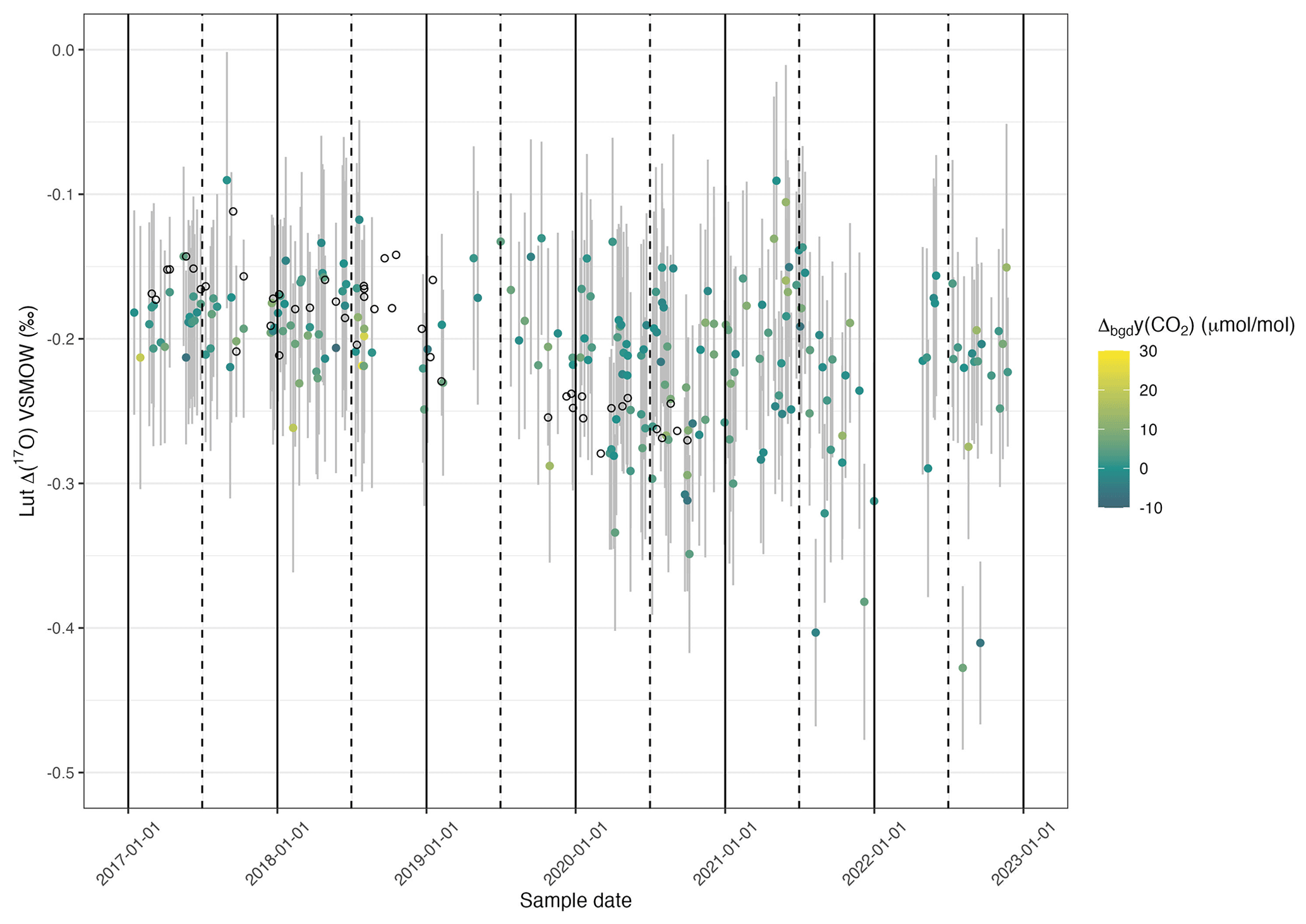
Figure C2 Δ(¹⁷O) record for Lutjewad from SICAS flask measurements (filled circles) and DI-IRMS flask measurements of duplicate flasks from the IMAU (open circles). The combined uncertainties of the SICAS measurements are shown as the grey error bars (±1σ) and include the measurement uncertainty, repeatability, accuracy and introduced uncertainty as a consequence of the calibration method used. The difference in amount fraction between the sample and the background curve, ΔCO₂, is indicated by the colour of the data point.

Appendix D: Lutjewad Δ(¹⁷O) seasonality plots

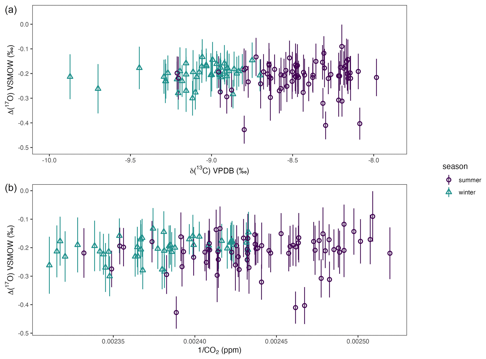
Figure D1 Δ(¹⁷O) summer (July, August and September) and winter (January, February and March) values for Lutjewad plotted against δ(¹³C) (a) and 1 $/$ CO₂ (b). The uncertainty bars show the combined uncertainty (±1σ) of the Δ(¹⁷O) SICAS measurements.

Appendix E: Estimation of the Δ(¹⁷O) depletion due to the equilibration of CO₂ and plant water

In this analysis, we make an estimate of the potential change in Δ(¹⁷O) as the result of the equilibration of atmospheric CO₂ and plant water. The δ(¹⁸O) value of atmospheric CO₂ is the result of multiple processes, but, for simplicity, we assume that the value is fully the result of the equilibration of CO₂ and plant water. The highest δ(¹⁸O) for CO₂ measured in the Lutjewad record is 42.48 ‰ (VSMOW). To derive a value of 42.48 ‰ assuming a fractionation factor of 1.0412 for CO₂–H₂O equilibration, the leaf water has to have a δ(¹⁸O) of 1.23 ‰. Soil water in the Netherlands typically has a δ(¹⁸O) of −7.5 ‰ (VSMOW) (Mook, 1970). We assume that the change in δ(¹⁸O) between the soil water and the plant water is caused by evapotranspiration (the fractionation factor is 0.9917; West et al., 2008) where θ is 0.516, the lowest value that was found by Landais et al. (2006). This will result in plant water with a δ(¹⁷O) of 0.56 ‰ and a Δ(¹⁷O) of −0.1 ‰. This Δ(¹⁷O) value will translate to the CO₂ that equilibrates with the water.