Evaluating modelled tropospheric columns of CH₄, CO, and O₃ in the Arctic using ground-based Fourier transform infrared (FTIR) measurements

This study evaluates tropospheric columns of methane, carbon monoxide, and ozone in the Arctic simulated by 11 models. The Arctic is warming at nearly 4 times the global average rate, and with changing emissions in and near the region, it is important to understand Arctic atmospheric composition and how it is changing. Both measurements and modelling of air pollution in the Arctic are difficult, making model validation with local measurements valuable. Evaluations are performed using data from five high-latitude ground-based Fourier transform infrared (FTIR) spectrometers in the Network for the Detection of Atmospheric Composition Change (NDACC). The models were selected as part of the 2021 Arctic Monitoring and Assessment Programme (AMAP) report on short-lived climate forcers. This work augments the model–measurement comparisons presented in that report by including a new data source: column-integrated FTIR measurements, whose spatial and temporal footprint is more representative of the free troposphere than in situ and satellite measurements. Mixing ratios of trace gases are modelled at 3-hourly intervals by CESM, CMAM, DEHM, EMEP MSC-W, GEM-MACH, GEOS-Chem, MATCH, MATCH-SALSA, MRI-ESM2, UKESM1, and WRF-Chem for the years 2008, 2009, 2014, and 2015. The comparisons focus on the troposphere (0–7 km partial columns) at Eureka, Canada; Thule, Greenland; Ny Ålesund, Norway; Kiruna, Sweden; and Harestua, Norway. Overall, the models are biased low in the tropospheric column, on average by −9.7 % for CH₄, −21 % for CO, and −18 % for O₃. Results for CH₄ are relatively consistent across the 4 years, whereas CO has a maximum negative bias in the spring and minimum in the summer and O₃ has a maximum difference centered around the summer. The average differences for the models are within the FTIR uncertainties for approximately 15 % of the model–location comparisons.

1 Introduction

Short-lived climate forcers (SLCFs) are a group of greenhouse gases and air pollutants with lifetimes less than 2 decades (IPCC, 2021). These include methane (CH₄), ozone (O₃), black carbon, halocarbons, sulfate, nitrate, and organic aerosols. The Intergovernmental Panel on Climate Change (IPCC) reports that in addition to radiative forcing, SLCFs have been found to have negative impacts on air quality, ecosystems, and human health. Due to their relatively short lifetimes, SLCFs are generally reflective of emission rates, meaning that mitigation can result in near-term impacts. Understanding the influences of SLCFs on the future climate will aid in policies and mitigation strategies to stay on track with the Paris Accord and its subsequent amendments. Reductions in SLCFs can be particularly beneficial in the Arctic because models have demonstrated a strong climate response in this region to local and remote forcing by SLCFs (Stohl et al., 2015).

The Arctic Monitoring and Assessment Programme (AMAP) was created by the Arctic Council to provide science-based analysis of Arctic pollution and climate change. AMAP has provided reports on SLCF impacts on the Arctic dating back to 2008. The 2021 AMAP SLCF assessment report assesses the impacts of black carbon, CH₄, O₃, and sulfate aerosols on the air quality, climate, and human health in the Arctic region (AMAP, 2021). A key difference from previous AMAP reports is the emphasis on air quality and human health. In addition to these SLCFs, the analysis includes the SLCF precursor gases carbon monoxide (CO), nitric oxide (NO), and nitrogen dioxide (NO₂). The report compares the output from 18 models with various historical measurements, including satellite, aircraft, ship, and in situ datasets. These observations are used to assess what processes need to be revised in the models and how these shortcomings impact the further application of the models, such as for climate and health predictions. Other chapters explore emissions, measurement advances, trends, climate air quality impacts, health ecosystem impacts, and next steps. A prominent theme in this report is the severity of change happening in the Arctic. This includes the amplification of the pace of change in physical drivers, such as temperature and snow cover, and the frequency of extreme events, such as wildfires and incidents of rapid sea-ice loss. These factors contribute to ecosystem disruption, directly affecting local Arctic communities, in addition to having global repercussions. SLCF reductions are motivated by the near-term (20–30 years) benefits and by the goal of slowing the warming of the Arctic climate, which results in more wildfires and permafrost melt and, in turn, an increase in SLCF emissions and precursor gases (AMAP, 2021). The projections in this report provide guidance, objectives, and cautions for potential reduction implementation scenarios (AMAP, 2021). This study builds upon the model–measurement comparisons presented in the 2021 AMAP SLCF assessment report using an additional Arctic dataset that was not included in the original report.

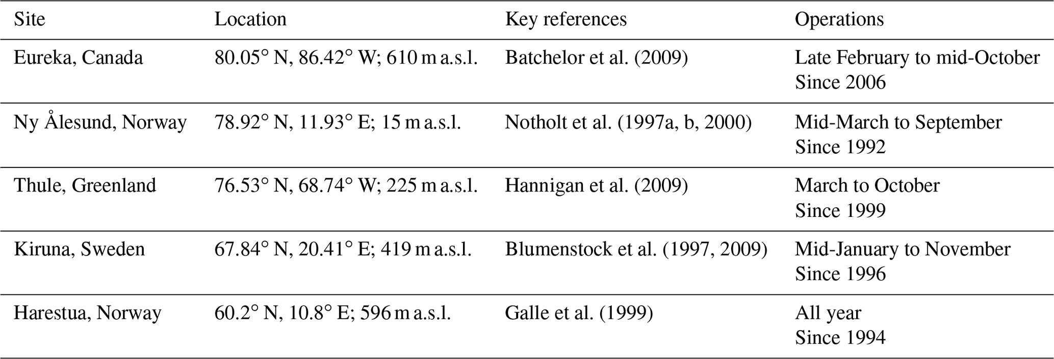
The atmospheric measurements used to evaluate the models presented in this paper were made by Fourier transform infrared (FTIR) spectrometers that are contributing members of the Network for Detection of Atmospheric Composition Change (NDACC). NDACC has over 70 stations around the globe, collecting high-quality atmospheric composition measurements with ground-based, remote-sensing instruments (De Mazière et al., 2018). The network's objective is to create a long-term database for various studies such as atmospheric trends, assessing links between climate and air quality, and as a resource for other atmospheric investigations such as satellite validation and model development. Atmospheric vertical profiles and trace gas columns are retrieved from high-resolution FTIR spectrometers that record solar spectra featuring characteristic atmospheric absorption lines. Five of the 28 NDACC FTIR stations are located at latitudes north of 60^∘ N; for the purpose of this study, these will all be referred to as Arctic sites. The five sites are Eureka, Canada; Ny Ålesund, Norway; Thule, Greenland; Kiruna, Sweden; and Harestua, Norway. These high-latitude NDACC FTIR instruments provide a valuable set of long-term, measurements of multiple species of interest in the Arctic. Compared to surface in situ or satellite observations, the column-integrated FTIR measurements have a spatial and temporal footprint that is more representative of the free troposphere. Performing model–measurement comparisons with partial column data supports and thus complements the assessments presented in the 2021 AMAP report. Previous studies have used FTIR data to examine model biases in the Arctic (e.g., Wespes et al., 2012; Zhou et al., 2019; Mahieu et al., 2021).

Measurements in the Arctic are difficult due to the harsh environment, remote locations, and high operating costs, resulting in a scarcity of monitoring stations and a limited representation of atmospheric vertical information. Using measurements to evaluate model simulations of the Arctic is important because the latter are used to project future changes in the Arctic, a region that is sensitive to climate change, warming at a rate 3 to 4 times the global average (Bush and Lemmen, 2019; Ballinger et al., 2020; AMAP, 2021; IPCC, 2021; Rantanen et al., 2022). These factors have led to initiatives like the AMAP SLCF assessment and the POLARCAT (Polar Study using Aircraft, Remote Sensing, Surface Measurements and Models, of Climate, Chemistry, Aerosols and Transport) Model Intercomparison Project (POLMIP), which, in part, aim to assess model performance in the Arctic region. POLMIP examined 11 atmospheric models in relation to a variety of Arctic observations taken as part of the International Polar Year in 2008 (Emmons et al., 2015). AMAP and POLMIP, in addition to the subsequent complementary publications (i.e., Wespes et al., 2012; Emmons et al., 2015; Monks et al., 2015; Whaley et al., 2022, 2023), provide a valuable point of reference for the modelling of CH₄, CO, and O₃ in the Arctic, which is explored in this paper. This allows for the findings presented here to be appraised relative to results from the same models compared to other instruments, with differing temporal frequency and altitude ranges (i.e., Whaley et al., 2022, 2023), with different simulations and Arctic FTIR measurements (i.e., Wespes et al., 2015), and to generally assess the similarities and differences that arise within Arctic SLCF modelling.

This project examines simulations from 11 models that were run for the 2021 AMAP SLCF assessment report, to assess the agreement between modelled trace gas concentrations and ground-based retrievals from high-latitude FTIR spectrometers. Specifically, this paper presents comparisons of CH₄, CO, and O₃ partial columns (from 0 to 7 km) for the years 2008, 2009, 2014, and 2015. The models examined are chemical transport and climate models: CESM, CMAM, DEHM, EMEP MSC-W, GEM-MACH, GEOS-CHEM, MATCH, MATCH-SALSA, MRI-ESM2, UKESM1, and WRF-CHEM. The objective is to utilize the high-quality, long-term Arctic FTIR datasets to assess how well the models perform. The remainder of this paper is organized as follows: Sect. 2 provides a description of the datasets used, Sect. 3 describes the analysis methodology, Sect. 4 examines the results and compares them with similar studies, and Sect. 5 presents the summary and conclusions.

2 Datasets

2.1 FTIR spectroscopy and retrievals

The FTIR measurement sites included in this study are summarized in Table 1, and the data are publicly available in the NDACC data repository (https://www-air.larc.nasa.gov/missions/ndacc/data.html, last access: 14 February 2023). These instruments require sunlight and a clear sight to the sun to make measurements, and so the high-latitude datasets are limited to the sunlit portion of the year at each location. To ensure high data quality and consistency between sites, NDACC has several specialized instrument and theme groups; the instruments used here are part of the Infrared Working Group (IRWG). The 10 standard gases reported by sites participating in the IRWG are C₂H₆, CH₄, CO, ClONO₂, HCl, HCN, HF, HNO₃, N₂O, and O₃, while several other gases are retrieved as research data products, including C₂H₂, CH₃OH, H₂CO, HCOOH, and OCS. The FTIR measurements cycle through a series of optical filters covering different spectral regions between approximately 650 and 4500 cm⁻¹ for the retrieval of multiple atmospheric gases. Atmospheric trace gas profiles and columns are retrieved with the SFIT4 algorithm, using optimal estimation to iteratively adjust an a priori profile to match a modelled spectrum to the measured spectrum within a defined convergence criterion (Rodgers, 2000; IRWG, 2020). The a priori profile information for the modelled spectra is provided by 40-year-average profiles from the Whole Atmosphere Community Climate Model (WACCM) (Marsh et al., 2013), with spectroscopic absorption parameters from the HITRAN 2008 line list (Rothman et al., 2009) and daily pressure and temperature profiles from the U.S. National Centers for Environmental Prediction (NCEP) (Kalnay et al., 1996). All sites included in this paper use SFIT4, except Kiruna, which uses a comparable retrieval code called PROFFIT, which has been shown to agree well with SFIT2 (which preceded SFIT4) (Hase et al., 2004). Primary references and further details of the sites are presented in Table 1.

Table 1 Summary of NDACC FTIR sites used in this study.

The NDACC FTIR data files include the volume mixing ratio (VMR) in parts per million (ppm) and total columns and partial columns in molecules per centimeter squared (molec. cm⁻²). Other variables include altitude, date and time of observation, pressure, the a priori vertical profile, the averaging kernel (AVK) matrix, and retrieval uncertainties, both systematic and random. The random uncertainties are determined from the temperature, solar zenith angle, and measurement noise from the signal-to-noise ratio. Systematic uncertainties are determined from temperature and line parameters such as line strength and width.

The averaging kernel matrix represents the relationship between the retrieved state and the true atmospheric state at each altitude layer, and the sensitivity of a retrieval is calculated by taking the sum of the rows of the averaging kernel. This indicates how much of the information is coming from the a priori profile and how much comes from the measurement itself (Rodgers, 2000; Vigouroux et al., 2009). The degrees of freedom for signal (DOFS) are calculated by taking the trace of the averaging kernel; this indicates the number of independent pieces of information coming from each retrieval or, inversely, the number of components not constrained by the a priori profile information. The random and systematic FTIR partial column uncertainties are calculated using the error covariance matrices, following the method outlined in Vigouroux et al. (2009). The square root of the associated error is taken, and this is scaled to a percent uncertainty using the corresponding partial column sum. The mean systematic and random percent errors are added in quadrature to get the overall mean percent uncertainty for the species. The number of measurements, mean DOFS, and mean percent uncertainty in the 0–7 km partial columns of CH₄, CO, and O₃ for 2008, 2009, 2014, and 2015, for each station, are listed in Table 2. The mean partial column (0–7 and 7–20 km) and total column averaging kernels for CH₄, CO, and O₃ for 2008, 2009, 2014, and 2015, are shown in Fig. 1. The lowest-level difference between Kiruna and the other locations results from the use of a stronger constraint for the lowest level with the PROFFIT retrieval; however, retrieval error and noise indicate that the agreement between the averaging kernels (AVKs) is reasonable (Hase et al., 2004). The DOFS and averaging kernels are indicators of the vertical information within a retrieval. Figure 1 shows that the mean partial column averaging kernels for 0–7 and 7–20 km are distinguishable, with maxima at different altitudes. The mean total column averaging kernels for all three species appear smooth around 1.0, which indicates that contributions from all altitudes have similar weights in the total column. By altitude, the sensitivity of each species is >0.5 in the partial column examined (not shown), meaning that more than half of the retrieved profile information comes from the measurement (Vigouroux et al., 2009). The average DOFS vary by species and station, given the reduced column height of 0–7 km; some of the values are less than 1, meaning the retrieval is somewhat constrained by the a priori profile. However, it should be noted that the comparisons presented in this paper account for the vertical sensitivity of the FTIR measurements by smoothing the model data with the averaging kernels. This process is described in Sect. 3.

Table 2 Summary of FTIR measurement statistics.

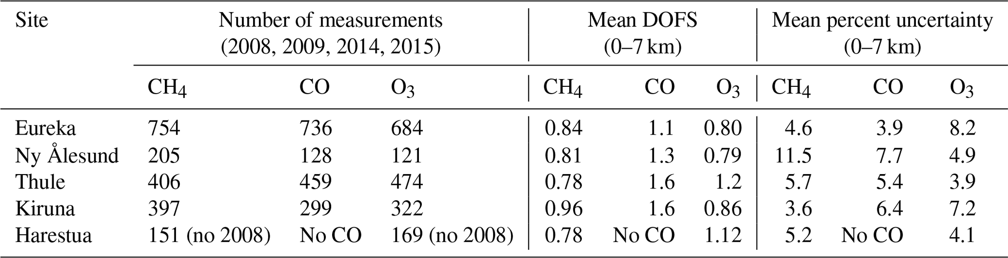
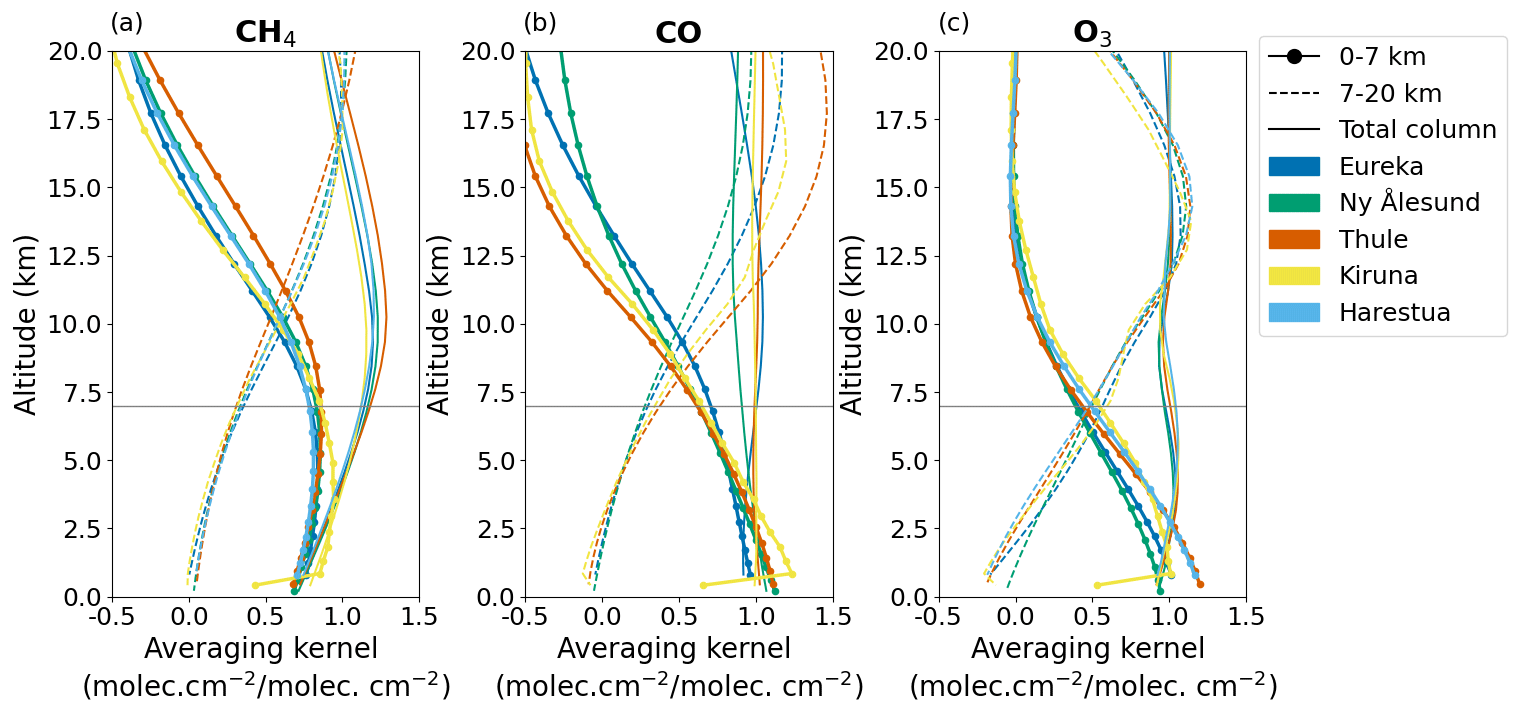
Figure 1 Mean 0–7 km partial column averaging kernels (lines with circle markers), mean 7–20 km partial column averaging kernels (dashed lines), and mean total column averaging kernels (solid lines), all in units of (molec. cm⁻² (molec. cm⁻²)⁻¹), by altitude, for (a) CH₄, (b) CO, and (c) O₃. Means are for 2008, 2009, 2014, and 2015 for all five FTIR sites except Harestua (no 2008 data).

2.2 Atmospheric models

The models used in this study provide three-dimensional VMR fields on 3-hourly intervals for 2008, 2009, 2014, and 2015. These 4 years were selected for the 2021 AMAP SLCF assessment; 2008 and 2009 were previously evaluated in the 2015 AMAP report, and 2014 and 2015 were added to include more recent results from years for which Arctic measurements were available at the time (AMAP, 2021). The gases CH₄, CO, and O₃ were chosen for this study as model output for these species was available at 3-hourly intervals, and the FTIR measurements have good sensitivity for them throughout the 0–7 km with the FTIR, as discussed in the previous section. Note that not every model has provided all three gases; there are 3 which have CH₄, 9 with CO, and 11 with O₃ (see Table 3). The model simulations are the same as those discussed in Whaley et al. (2022, 2023) and the 2021 AMAP SLCF report; however, the analyses there were performed with the monthly mean output, while the analysis here is with the 3-hourly output, all of which is available at http://crd-data-donnees-rdc.ec.gc.ca/CCCMA/products/AMAP/ (last access: 14 February 2023). While more models participated in the AMAP SLCF assessment (18 total) and other species were simulated, these were not included in the current study because either the models did not have 3-hourly outputs or the FTIR retrievals had insufficient tropospheric sensitivity (e.g., NO₂).

Table 3 Summary of the models used in this study.

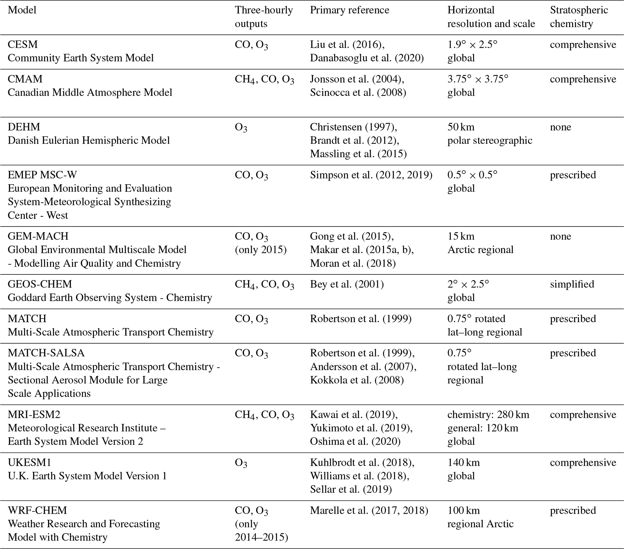
This set of models is a mix of Earth system models, chemical transport models, global transport models, and chemistry climate models. The models all used the same set of anthropogenic emissions from ECLIPSE v6b (Evaluating the Climate and Air Quality Impacts of Short-Lived Pollutants) by the IIASA GAINS (International Institute for Applied Systems Analysis – Greenhouse gas – Air pollution Interactions and Synergies) model (Amann et al., 2011; Klimont et al., 2017; Höglund-Isaksson et al., 2020). However, the models differ in their use of biogenic and volcanic emissions, tropospheric gas-phase chemistry complexity, and vertical and horizontal grids. Four of the 11 models simulate the stratosphere fully, one (GEOS-Chem) uses a simplified linearized stratospheric chemistry, one (GEM-MACH) only simulates the troposphere, and the rest use prescribed climatologies at the stratospheric boundary (Whaley et al., 2022). In total, 9 of the 11 models examined use the Global Fire Emissions Database (GFED; van der Werf et al., 2017) or GFED-based (CMIP6) forest fire emissions, and 9 of the 11 exclusively use ECLIPSEv6b for agricultural waste burning. A summary of the models is presented in Table 3, including which gases are examined in this study, their resolution, and to what degree stratospheric chemistry is considered. It should be noted that the CH₄ concentrations in these models have been prescribed (Whaley et al., 2022). The prescribed concentrations are input at the bottom model layer, and all come from the same dataset (Prather et al., 2012; Olivié et al., 2021), but the resulting CH₄ partial columns differ based on the processes within each model. For a full description of the models, see Appendix A of Whaley et al. (2022) and the references in Table 3.

3 Methods

As mentioned, the models provided 3-hourly VMRs on model-specific pressure levels and latitude–longitude grids. The process of aligning the model output to FTIR data is described by the flow chart in Fig. 2.

Figure 2 Flow chart depicting the process of matching model output to FTIR data.

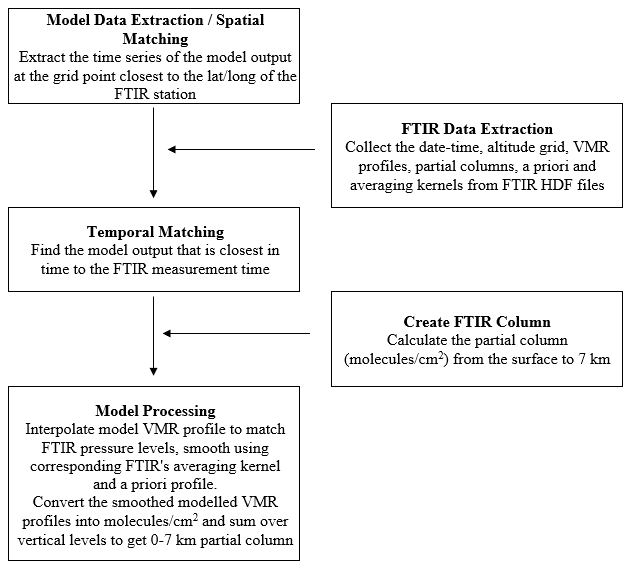
This procedure modifies the model output to correspond to an FTIR measurement, making the resulting partial columns equivalent for further comparison. The date and time and volume-mixing-ratio profiles from the model output are extracted from the grid point that is closest to the FTIR location. The FTIR measurements are matched with the 3-hourly model measurement closest in time (± <1.5 h); this is done to minimize the time difference between the two points, such that no measurement is greater than 1.5 h from a modelled output. If more than one FTIR measurement coincides with a model output (i.e., multiple measurements are within 1.5 h of the same model time), the FTIR measurements are averaged. After the model outputs are matched to the FTIR measurements, they are interpolated onto the pressure grid of the FTIR profile. Then, the model VMR profile is smoothed using the respective FTIR measurement's averaging kernel and a priori profile. The purpose of smoothing the model data with the FTIR averaging kernel is to adjust the model to the vertical sensitivity of the FTIR measurement (Rodgers and Connor, 2003). The calculation for the smoothing is shown in Eq. (1), where x_a is the FTIR a priori VMR vertical profile, A is the VMR averaging kernel matrix from the corresponding FTIR measurement, and x_model is the modelled VMR vertical profile:

$$\begin{array}{}\text{(1)}& {\mathit{x}}_{\mathrm{smooth}}={\mathit{x}}_{\mathrm{a}}+\mathbf{A}\times \left[{\mathit{x}}_{\mathrm{model}}-{\mathit{x}}_{\mathrm{a}}\right].\end{array}$$

The model VMR profile is then transformed to a layer profile in units of molecules per centimeter squared using the ratio between the VMR and layer partial column (in molecules per centimeter squared) in the retrieved FTIR profile as the conversion factor. At this point, the model output has the same altitude grid and units as the FTIR retrieval, which allows for partial columns to be summed. Partial columns from 0 to 7 km were calculated given AMAP's focus on SLCFs in the troposphere, with the cap at 7 km chosen to limit any stratospheric influence. Note that “0 km” is used as proxy for the minimum altitude, but this varies, based on location, with the altitude of each instrument listed in Table 1. The partial column examined here (0–7 km) encompasses 11 vertical layers for all sites, except Ny Ålesund, which has an additional (12th) layer given the lower altitude of its location (see Table 1).

To compare the model and FTIR partial columns, a model–measurement percent difference (Δ_i) is calculated, as defined by Eq. (2) for a single model–measurement pair (i), where PC_M,i and PC_F,i are the 0–7 km partial columns for the model and FTIR, respectively:

$$\begin{array}{}\text{(2)}& {\mathrm{\Delta }}_i=\left({\displaystyle \frac{{\text{PC}}_{\mathrm{M},i}-{\text{PC}}_{\mathrm{F},i}}{{\text{PC}}_{\mathrm{F},i}}}\right)\times \mathrm{100}.\end{array}$$

A regression line is fit to the raw scatter plot data of the model output versus FTIR measurements using all the available data points, where each plot includes the equation of this line and the correlation coefficient, R². The normalized root mean square error (NRMSE), given by Eq. (3), is presented for each model and location, where N is the total number of model–measurement pairs (Kärnä and Baptista, 2016). The root mean square error is normalized to the standard deviation of the FTIR data (σ_F) used in the respective analysis:

$$\begin{array}{}\text{(3)}& \text{NRMSE}={\displaystyle \frac{\mathrm{1}}{{\mathit{\sigma }}_{\mathrm{F}}}}\sqrt{\left[{\sum }_{i=\mathrm{1}}^N{\left({\text{PC}}_{\mathrm{M},i}-{\text{PC}}_{\mathrm{F},i}\right)}^{\mathrm{2}}\right]}.\end{array}$$

In addition to evaluating the models using every available FTIR data point in the analysis years, the monthly mean annual cycles are also presented. The monthly mean partial columns (PC${}_{\mathrm{F},\mathrm{monthly},j}$) are calculated by taking the mean of every measurement in a given month (j), where N_j is the number of points included in the month for all years considered. The monthly model mean partial columns (PC${}_{\mathrm{M},\mathrm{monthly},j}$) are made in the same manner, using only the smoothed partial columns that have a corresponding matching FTIR measurement, as defined above. Equation (4) outlines the calculation of a monthly mean partial column for month j for (a) the FTIRs (PC${}_{\mathrm{F},\mathrm{monthly},j}$) and (b) the models (PC${}_{\mathrm{M},\mathrm{monthly},j}$):

$$\begin{array}{}\text{(4a)}& {\displaystyle }{\text{PC}}_{\mathrm{M},\mathrm{monthly},j}={\displaystyle \frac{\mathrm{1}}{N_j}}{\sum }_{i=\mathrm{1}}^{N_j}{\text{PC}}_{\mathrm{M},i},\text{(4b)}& {\displaystyle }{\text{PC}}_{\mathrm{F},\mathrm{monthly},j}={\displaystyle \frac{\mathrm{1}}{N_j}}{\sum }_{i=\mathrm{1}}^{N_j}{\text{PC}}_{\mathrm{F},i}.\end{array}$$

The model–measurement monthly mean percent difference (Δ_monthly,j), shown by Eq. (5), follows the same process as the monthly mean partial column and is the mean value from Eq. (2) for each month (j) across the years, where the error bars on the monthly mean plots represent the standard deviation of this mean:

$$\begin{array}{}\text{(5)}& {\mathrm{\Delta }}_{\mathrm{monthly},j}={\displaystyle \frac{\mathrm{1}}{N_j}}{\sum }_{i=\mathrm{1}}^{N_j}{\mathrm{\Delta }}_i.\end{array}$$

The mean of these monthly mean differences is used to calculate the overall mean percent difference (Δ_O) for each model, sometimes referred to as model bias, where N_months is the number of measurement months in a calendar year at that location (see Table 1), and the uncertainty given is the standard deviation of this mean:

$$\begin{array}{}\text{(6)}& {\mathrm{\Delta }}_{\mathrm{O}}={\displaystyle \frac{\mathrm{1}}{N_{\mathrm{months}}}}{\sum }_{j=\mathrm{1}}^{N_{\mathrm{months}}}{\mathrm{\Delta }}_{\mathrm{monthly},j}.\end{array}$$

Finally, the monthly multi-model mean (MMM) partial column for month j (PC${}_{\mathrm{MMM},\mathrm{monthly},j}$) is calculated by taking the mean PC${}_{\mathrm{M},\mathrm{monthly},j}$ for all models, at a given location, calculated with Eq. (4b), and the MMM monthly mean difference (${\mathrm{\Delta }}_{\mathrm{MMM},\mathrm{monthly},j}$) is the mean of Δ_monthly,j for all models, at a given location, calculated with Eq. (5). The overall percent difference in the MMM measurement (Δ_O,MMM) is given by Eq. (7):

$$\begin{array}{}\text{(7)}& {\mathrm{\Delta }}_{\mathrm{O},\mathrm{MMM}}={\displaystyle \frac{\mathrm{1}}{N_{\mathrm{months}}}}{\sum }_{j=\mathrm{1}}^{N_{\mathrm{months}}}{\mathrm{\Delta }}_{\mathrm{MMM},\mathrm{monthly},j}.\end{array}$$

These steps are taken to establish the modelled seasonal cycles and quantify the differences between the models and measurements, by month and season. Further, assessing the MMM by month allows for a general overview of when and where models diverge from measurements and can help suggest shortcomings in the models. There are not enough measurements per day to evaluate a diurnal cycle, although it is expected to be small in the Arctic, and there are not enough years available in the 3-hourly dataset used here to examine long-term trends.

When discussing FTIR uncertainty, this refers to the mean uncertainty per gas and station, as listed in Table 2. When discussing the mean difference between the model and measurements, this refers to the overall mean difference (Δ_O) as described by Eq. (6). In Sects. 4 and 5, these two parameters are used to assess model performance: if Δ_O is within measurement (FTIR) uncertainty, the model can be considered in general agreement with the FTIR; if Δ_O± the standard deviation of the mean is within the measurement uncertainty, then the model is sometimes in agreement with the measurements; and if the uncertainty and Δ_O do not overlap, then the model and measurements do not agree.

4 Results and discussion

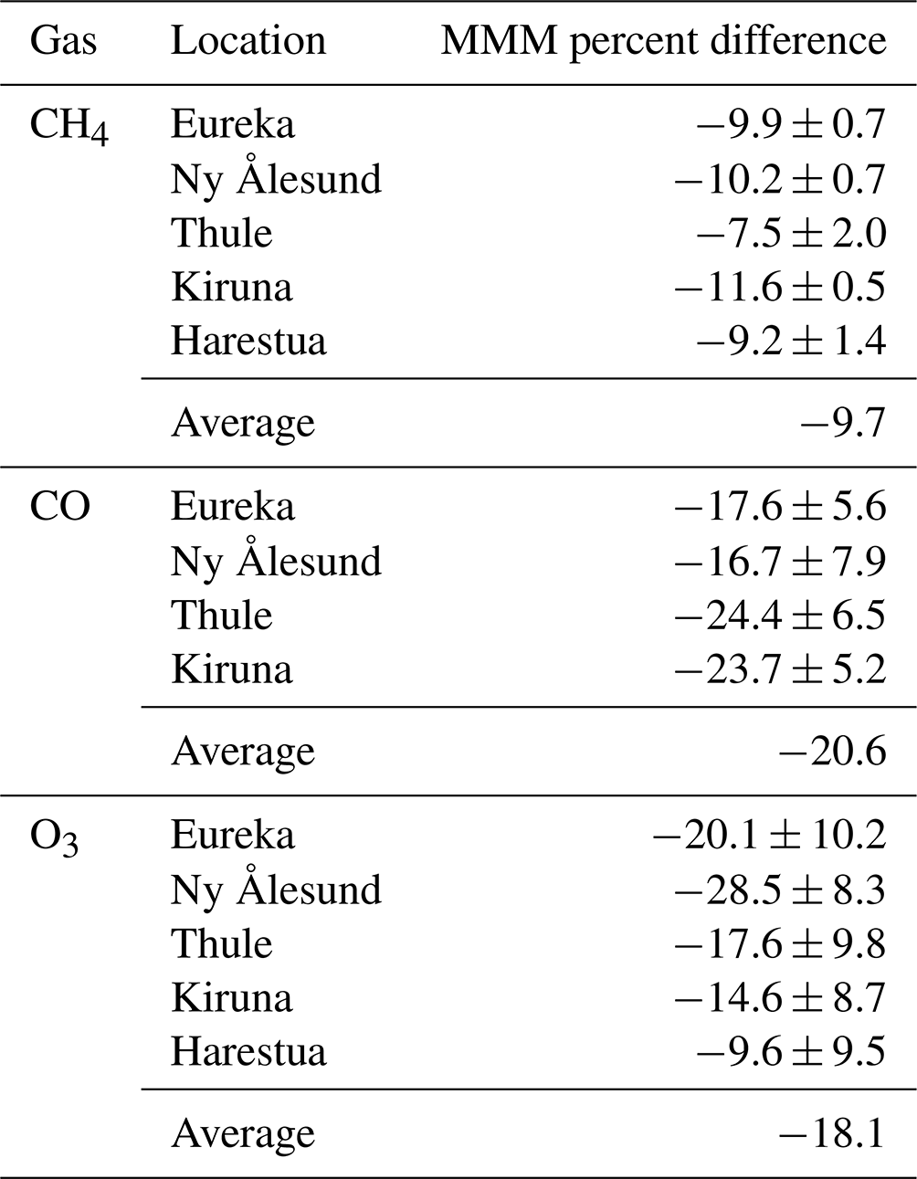
This section presents the analyses described above, for CH₄, CO, and O₃, and discusses the findings in the context of the 2021 AMAP SLCF assessment report and other related literature. Given the volume of data (three species, five locations, and 11 models), only selected plots are shown in the main text, with the remaining figures provided in Appendices A–C. These include plots for each location, showing the time series of the 0–7 km partial column for each measurement–model pair and the associated model–measurement percent difference, the equivalent plot reduced to monthly mean data (an individualized version of Figs. 3, 5, and 9), and the 0–7 km column of FTIR vs. smoothed model for the remaining locations (analogous to Figs. 4, 8, and 10). Figure 15 provides a summary of the overall differences for each model and location by species, as described by Eq. (6). Table 4 summarizes the overall MMM difference for each species at each location and the overall average for each species. All the comparisons shown are for a 0–7 km partial column, where the model output is smoothed as described by Eq. (1).

Table 4 The multi-model mean percent difference (Δ_O,MMM) for each species at each location, including the overall average percent difference for each species and the standard deviation of the mean.

4.1 CH₄

CH₄ is a powerful greenhouse gas (GHG), and its emissions are expected to increase in the Arctic due to melting permafrost (IPCC, 2021). CH₄ is also involved in the formation of tropospheric O₃, which is the third strongest anthropogenic GHG and an air pollutant at the surface. Therefore, it is important for both air quality and climate models to represent CH₄ accurately. The CH₄ plots for Ny Ålesund, Thule, Kiruna, and Harestua are provided in Appendix A, following the same order discussed here for Eureka.

Figure 3 shows the monthly mean 0–7 km partial column time series for the FTIR and models at each location (panels a–e), with the percent difference between the monthly mean model and monthly mean measurement for all locations shown in panel (f). This shows that, apart from a few outliers, the pattern of the seasonal cycle of CH₄ is consistent, although the amplitude is underestimated. The uniformity between the years (see Figs. A1–A5 for full data time series plots) and consistency of the model biases between sites is likely a consequence of CH₄ being prescribed in the models, in addition to the longer lifetime of CH₄, relative to the other SLCFs. This is also seen in Fig. 4 (and Figs. A11–A14), where the model and FTIR columns are compared, with the line of best fit and R² are indicated in the legend.

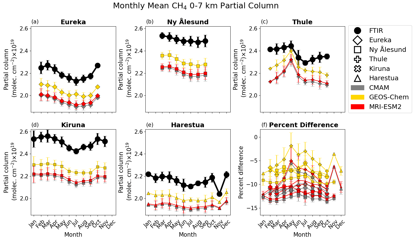
Figure 3 (a–e) Monthly mean FTIR (black) and smoothed model (colour) 0–7 km partial columns of CH₄ (PC${}_{\mathrm{F},\mathrm{monthly},j}$ and PC${}_{\mathrm{M},\mathrm{monthly},j}$, respectively), for each location, shown with the same y axis. Error bars represent the standard deviation of the monthly mean. (f) Mean model–measurement percent difference by month (Δ_monthly,j) for each model (by colour) and location (by marker). Error bars represent the standard deviation of the monthly mean percent difference.

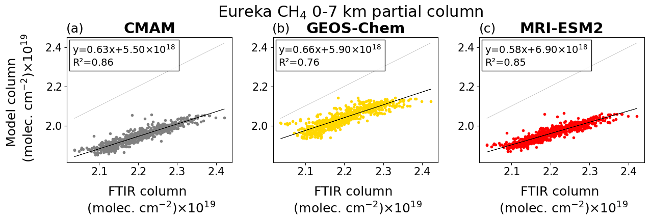
Figure 4 Smoothed model vs. FTIR 0–7 km partial columns of CH₄ for Eureka, showing all available model–FTIR corresponding data. The black line is the line of best fit, where the equation and R² are noted in the legend. The 1:1 line is shown in light grey.

A summary of the overall mean difference, R², and the normalized root-mean-square error for each location is shown in Fig. 5. Across all three models, Arctic CH₄ is underpredicted compared to the FTIR measurements. The surface in situ CH₄ comparison in Whaley et al. (2022) showed that measured surface CH₄ VMRs are much more variable than the modelled VMRs. However, in the 0–7 km partial columns in this study, CH₄ is well-mixed and more homogenous, resulting in better agreement between the models and the FTIR measurements. The low bias we find in this study for the Arctic sites is consistent with the global comparisons of these models to satellite measurements in Whaley et al. (2022), which found that some models did not distribute CH₄ with an accurate north–south gradient, resulting in low biases in the Arctic and high biases in lower latitudes. GEOS-Chem does simulate a north–south gradient, which is reflected in the smaller overall model–measurement percent difference, compared to other models, in all locations (note Fig. 6 in Whaley et al., 2022). However, the R² of GEOS-Chem vs. FTIR is smaller than that for the other models at some locations (Eureka and Kiruna), which can be attributed to the increase in variability the gradient introduces – including some instances of overestimation. The mean differences for each model across sites are relatively consistent, while the results vary more when comparing R² and NRMSE. Particularly, when comparing them between the same model, the R² for Ny Ålesund is the lowest and the NRMSE is the highest. The data from Ny Ålesund show less of a seasonal cycle than the other locations, and the FTIR uncertainty for CH₄ at Ny Ålesund is more than twice that of the other sites (see Fig. 15). The larger uncertainty may lead to reduced sensitivity to small changes and increased variability masking seasonal changes, which can contribute to the discrepancy between the models and observations. The mean difference for GEOS-Chem is within the uncertainty in the FTIR measurements for Ny Ålesund and Thule, as is the mean difference for MRI-ESM2 at Ny Ålesund; none of the other models are within the FTIR uncertainty at the given location (see Fig. 15).

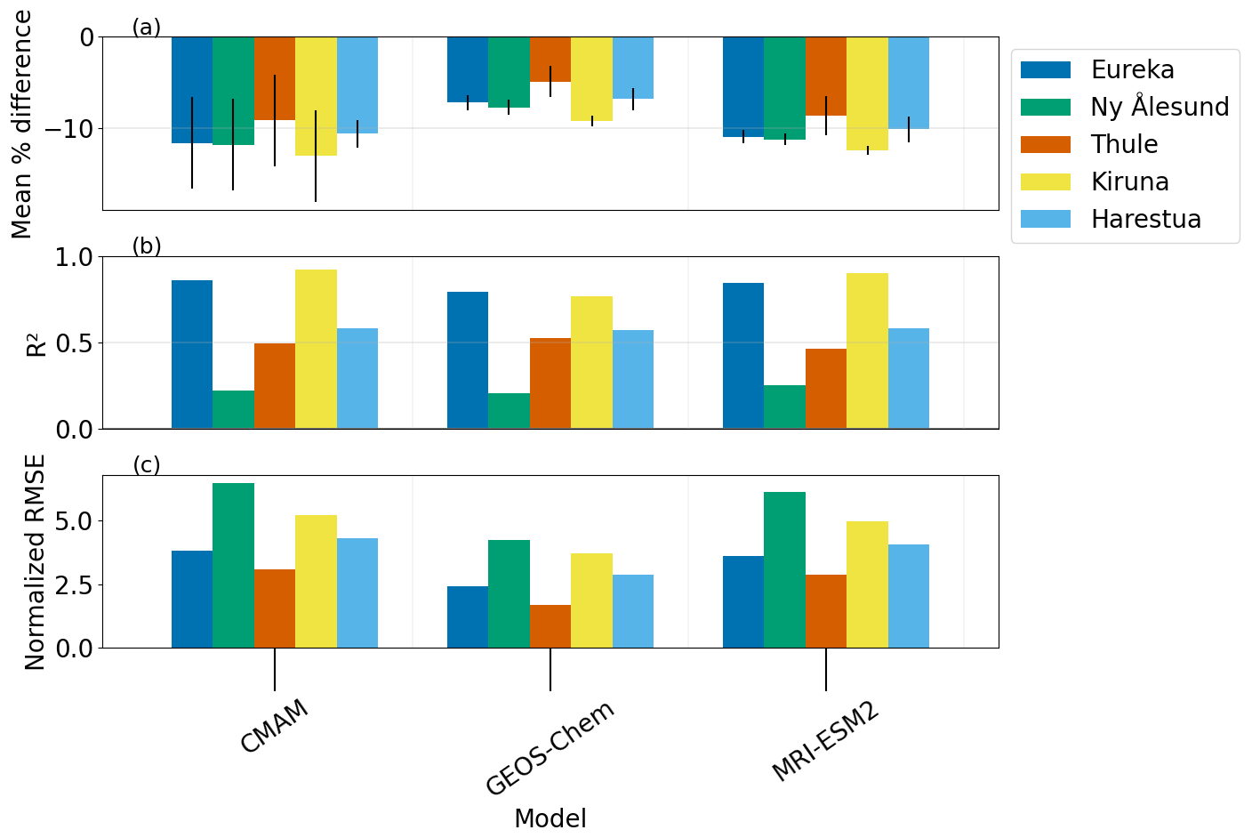
Figure 5 By model and location: (a) overall model–measurement mean percent difference for CH₄ 0–7 km partial columns (Δ_O), with error bars that represent the standard deviation of the mean, as shown in the legend of Figs. A6–A10; (b) R² as shown in Figs. 4 and A11–A14; (c) normalized root-mean-square error.

Figure 6 shows the multi-model mean (MMM) for each location and the percent difference compared to the monthly mean FTIR. The error bars and shading represent the standard deviation of the mean. The AMAP SLCF assessment report compares the models with surface CH₄ measurements and finds that the MMM bias for Arctic CH₄ is +1.3 % (AMAP, 2021). When comparing them with 0–7 km FTIR partial columns, the MMM bias ranges from −5% to −15 % (Fig. 6f) and unlike the results in the AMAP report, the comparisons are not improved by choosing a multi-model mean because all three models have a negative bias. The FTIR retrievals show good sensitivity to tropospheric CH₄ (sensitivity >0.5); however, as these column measurements average out CH₄ biases over the tropospheric column, they are not expected to exactly match the surface measurement comparisons. Furthermore, due to the sharp decrease in CH₄ above the tropopause (Whaley et al., 2022), a poor representation of the tropopause height may contribute to the low bias in the modelled 0–7 km partial columns, as shown from O₃ data in Whaley et al. (2023). The AMAP report also includes a comparison with upper-troposphere/lower-stratosphere (UTLS) CH₄ VMRs as measured by the ACE-FTS (Atmospheric Chemistry Experiment – Fourier Transform Spectrometer) satellite instrument and finds that the models are biased low by ∼ 100 ppbv in the vicinity of the tropopause (300 hPa; around ∼ 8–9 km), indicating that the modelled tropopause may be too low (Whaley et al., 2022). The results found here are consistent with Whaley et al. (2022), in that the model simulations of both the lower troposphere (0–7 km partial columns) and the UTLS are biased low, and models with north–south CH₄ gradients (here, only GEOS-Chem) have smaller biases than those that do not. Generally, the models can represent the temporal variability in the tropospheric column well, although they are biased low in magnitude, outside of the range of the FTIR uncertainty.

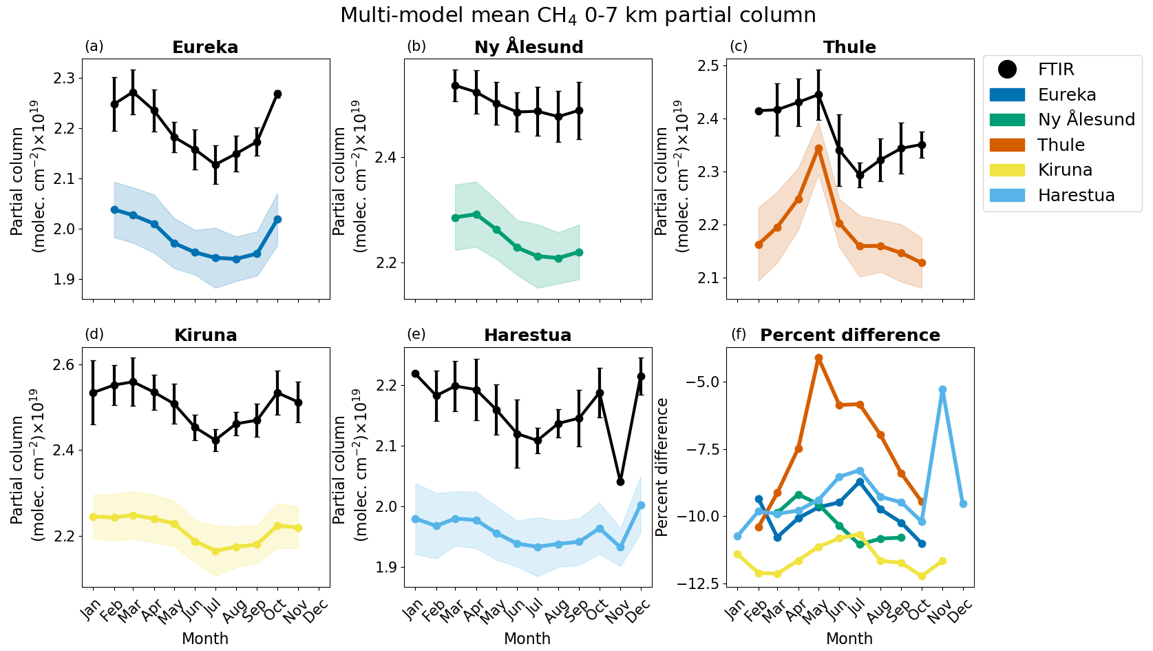
Figure 6 (a–e) Monthly mean FTIR (black) and multi-model mean (coloured) 0–7 km partial columns of CH₄ (PC${}_{\mathrm{F},\mathrm{monthly},j}$ and PC${}_{\mathrm{MMM},\mathrm{monthly},j}$, respectively), with error bars and shaded areas representing the standard deviation of the mean. (f) Monthly mean percent difference in the MMM (Δ_O,MMM) for all locations.

4.2 CO

Like CH₄, CO is involved in tropospheric O₃ formation in the presence of NO_x. Thus, in order to properly simulate tropospheric O₃, it is important for models to accurately simulate CO. In the Arctic, CO is used as a tracer for identifying and quantifying influences from biomass burning and lower-latitude anthropogenic emissions (e.g., Fisher et al., 2010; Monks et al., 2015; Viatte et al., 2015; Lutsch et al., 2020).

Nine of the 11 models examined in this study provided 3-hourly outputs for CO; WRF-Chem only has outputs for 2014 and 2015, and GEM-MACH only has data for 2015 (Table 3). Seven of the nine CO models examined use GFED-based fire emissions. The remaining models are EMEP MSC-W, which uses FINN fire emissions, and GEM-MACH, which uses CFFEPS fire emissions (Whaley et al., 2022). Evidence of biomass burning events can be observed in the summer months when examining the CO seasonal cycle with all available measurement points, where there are sporadic increases in the measured CO (Figs. B1–B4). The CO time series data (i.e., Figs. B1–B4 and 7/B5–B8) indicates that the GFED-based models may overestimate CO from biomass burning as their bias shifts positively in the summertime relative to the rest of the time series. This feature is absent for GEM-MACH, which does not have a consistent trend between sites during the summer (although results are only available for 1 year), and for EMEP MSC-W, which shifts more negatively in the summertime. It is well known that the fire emissions inventories vary greatly from each other (AMAP, 2021), causing these differences in model results.

Figure 7 and Figs. B5–B8 show the monthly mean partial columns and percent differences between the models and the FTIR measurements. This allows for an overview of the mean percent difference and how the model biases change over the year. For example, MATCH exhibits a positive shift in bias from the end of summer to the fall in all locations. WRF-Chem is biased low in the spring and summer but agrees better with the observations from August onwards, in contrast to EMEP-MSC-W, which tends to diverge from the measurements in the mid- to late summer. GEM-MACH is the only model that has a positive mean difference in all locations. The year-round difference is likely due to the fact that this model used anthropogenic emissions produced locally for most of its regional domain, instead of the ECLIPSEv6B anthropogenic emissions that all of the other models used, and lateral regional boundary conditions provided from MOZART4 (Model for Ozone and Related Chemical Tracers, version 4) global simulations (Emmons et al., 2010; Gong et al., 2018; AMAP, 2021). Further, Fig. 8 and Figs. B9–B11 show the correlations between the modelled and FTIR partial columns, with the line of best fit and R² indicated in the legend. For many models, the 1:1 correlation and Figs. 8 and B9–B11 show that models have better agreement with the FTIR for low CO values and the disparity increases as CO increases; i.e., the line of best fit and 1:1 line diverge. The points with the maximum CO VMRs correspond to the FTIR springtime peak in the CO cycle (since wintertime CO measurements are not possible during polar night).

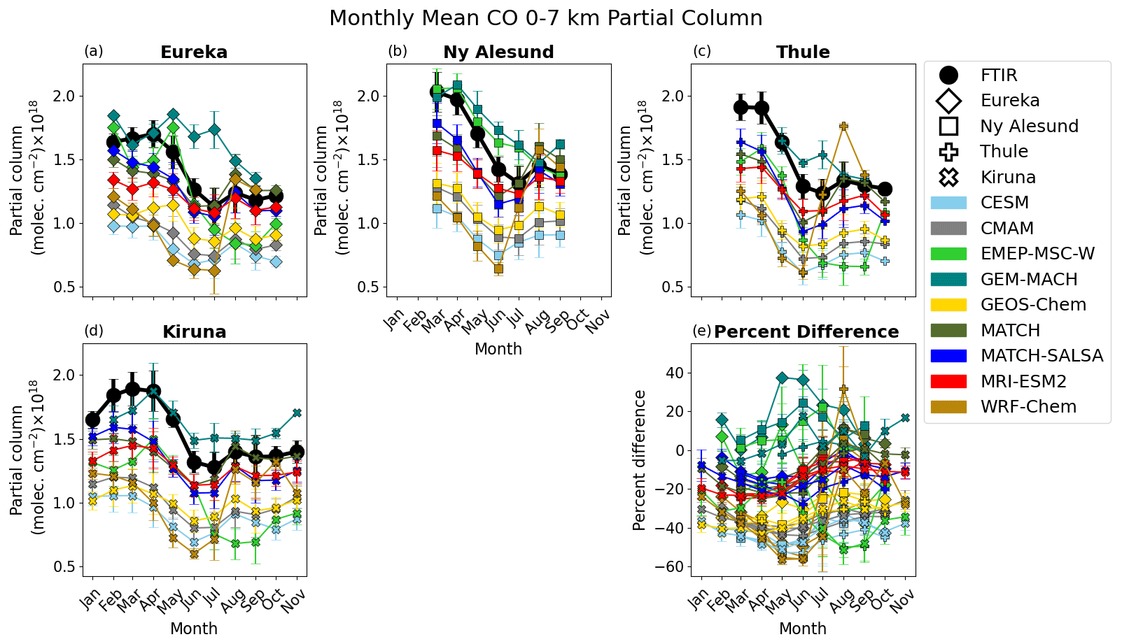
Figure 7 (a–d) Monthly mean FTIR (black) and smoothed model (colour) 0–7 km partial columns of CO (PC${}_{\mathrm{F},\mathrm{monthly},j}$ and PC${}_{\mathrm{M},\mathrm{monthly},j}$, respectively), for each location, shown with the same y axis. Error bars represent the standard deviation of the monthly mean. (e) Model–measurement mean percent difference by month (Δ_monthly,j) for each model (by colour) and location (by marker). Error bars represent standard deviation of the monthly mean percent difference.

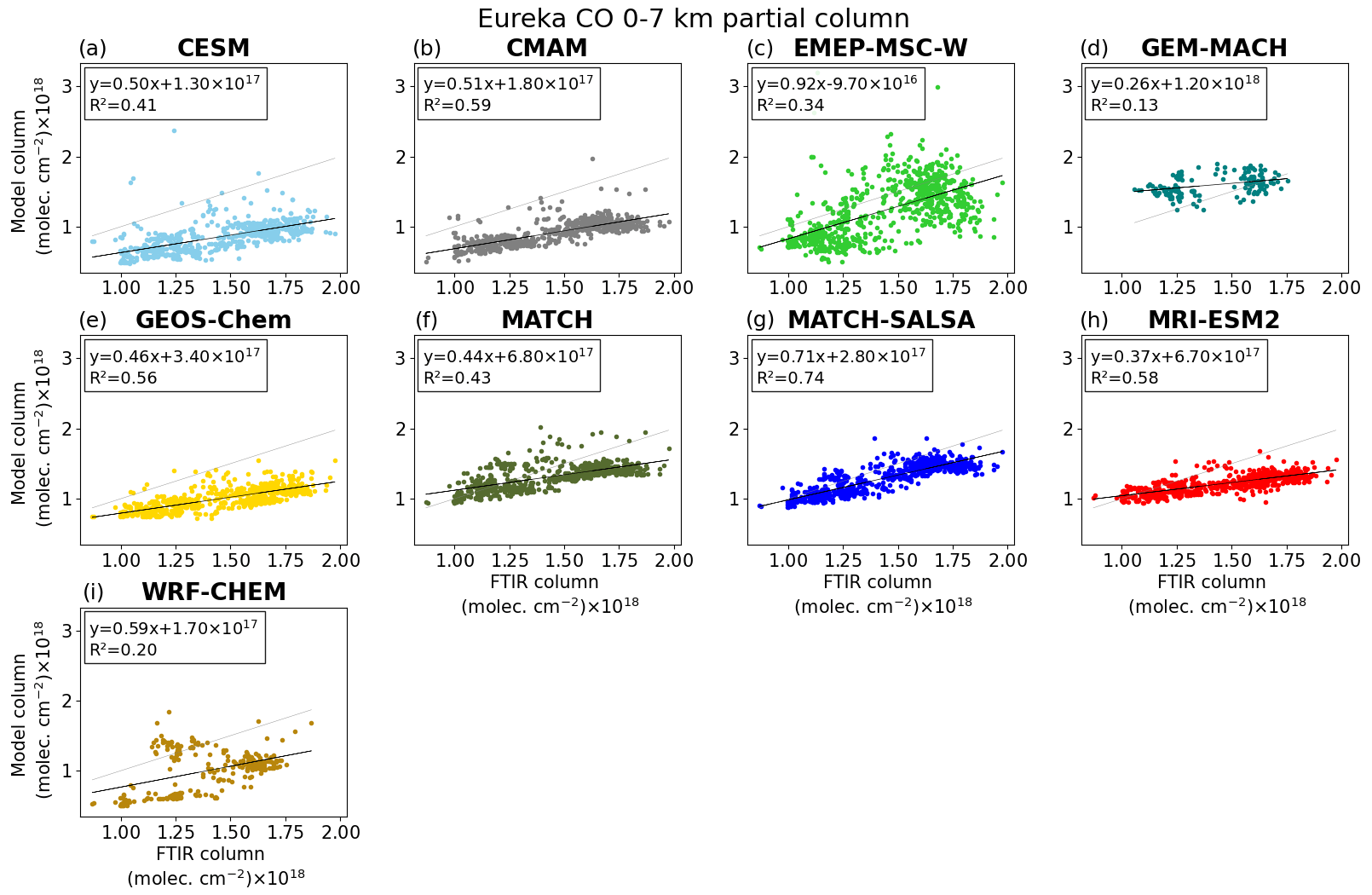
Figure 8 Smoothed model vs. FTIR 0–7 km partial column of CO for Eureka, showing all available model–FTIR corresponding data. The black line is the line of best fit, where the equation and R² are noted in the legend. The 1:1 line is shown in light grey.

Figure 9 summarizes the overall model–measurement mean percent difference R² and normalized root-mean-square error for all locations. GEM-MACH has a mean percent difference that is within the FTIR uncertainty for Thule and Kiruna; EMEP MSC-W and MATCH are simulated within the mean FTIR uncertainty for Ny Ålesund (see Fig. 15). MATCH-SALSA and MRI-ESM2 exhibit high R² and low percent difference across all locations, relative to the other models' values, although their columns do not fall within the FTIR uncertainties. GEM-MACH and MATCH have an NRMSE comparable to MATCH-SALSA and MRI-ESM2, despite generally lower R². WRF-Chem shows better agreement with the FTIR measurements from Eureka, where the NRMSE is comparable to CESM, CMAM, and GEOS-Chem. This is likely a result of the increased density of measurement points in August and September, when WRF-Chem exhibits a minimum bias compared to the FTIR data and because the comparison only includes data points from 2014 and 2015. The large negative biases earlier in the year lead to low R² and high NRMSE at all sites. This appears to be linked to negative biases in modelled surface CO over mid-latitude source regions and in the free troposphere compared to MOPITT data, as reported by Whaley et al. (2022). Overall, four model–location pairs have a mean difference within the average FTIR 0–7 km partial column uncertainty (see Table 2) and when including the standard deviation of the mean difference, an additional 8 pairs out of 36 meet this criterion.

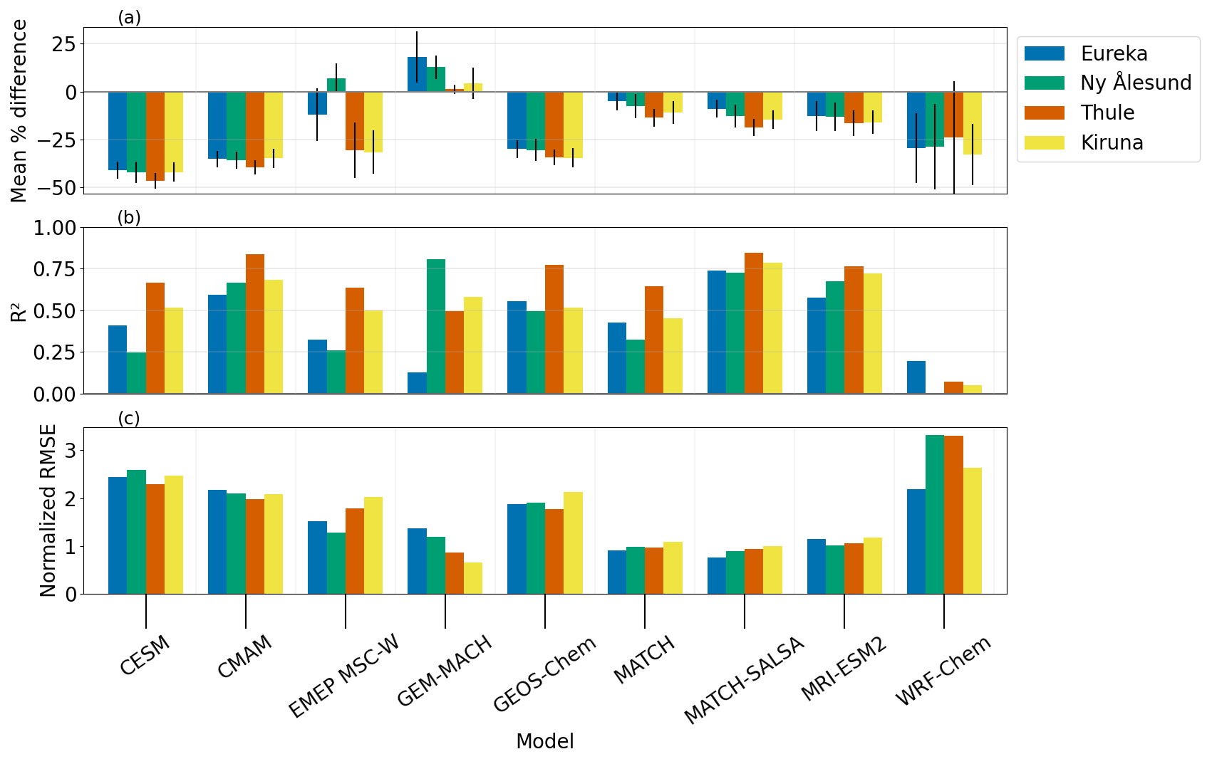
Figure 9 By model and location: (a) overall model–measurement mean percent difference for CO 0–7 km partial columns (Δ_O), with error bars that represent the standard deviation of the mean, as shown in the legend of Figs. B5–B8. (b) R² as shown in Figs. 8 and B9–B11. (c) Normalized root-mean-square error.

Figure 10 shows the monthly MMM for CO at each location, with the percent difference in the last panel (e). This highlights the general tendency of the models to underpredict tropospheric CO more in the spring than in the summer, which has been observed by other Arctic model–measurement comparison studies. The AMAP SLCF assessment report found that compared to CO from various surface networks, the models had a greater bias than for the other SLFCs examined, underestimating CO in the spring and overestimating CO in the summer (AMAP, 2021). The same pattern was observed when comparing them with MOPITT (Measurements of Pollution In The Troposphere) satellite CO in the free troposphere, at the 600 hPa level (Whaley et al., 2022). The change from a negative winter–spring bias to a positive summer bias was observed in model comparisons to surface CO measurements at two additional Arctic sites – Zeppelin, Norway, and Utqiaġvik (formerly Barrow), USA – with a −20% to 30 % bias in the first 6 months of the year (Whaley et al., 2023), which is compatible with results shown in Fig. 10e.

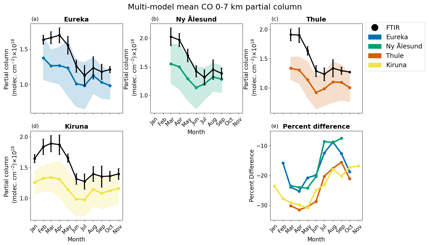
Figure 10 (a–d) Monthly mean FTIR (black) and multi-model mean (coloured) 0–7 km partial columns of CO (PC${}_{\mathrm{F},\mathrm{monthly},j}$ and PC${}_{\mathrm{MMM},\mathrm{monthly},j}$, respectively), with error bars and shaded areas representing the standard deviation of the mean. (e) Monthly mean percent difference in the MMM (Δ_O,MMM) for all locations.

In POLMIP, models were run for 2008 with a standardized emissions inventory; there is some overlap of models examined here, although a different emissions input was used (see Emmons et al., 2015, for full project description). Similarly to the results presented here, the POLMIP study found that relative to surface, airborne, and satellite Arctic tropospheric measurements, CO was underpredicted by the models (MMM gross error 9%–12%), with a more negative bias in the winter and spring compared to the summer, although the models still broadly captured the seasonal cycle (Monks et al., 2015). Using an idealized tracer, POLMIP examined anthropogenic and biomass burning influences in Arctic regions, demonstrating a seasonal dependence of transport efficiency. It was shown that for anthropogenic emissions, Europe influences the surface CO, while Asia and North America have more influence higher in the troposphere (Monks et al., 2015). Furthermore, the tracer investigation in that study showed that OH differences account for more variability between the models than the transport mechanisms within the individual models. However, it can be noted that although models may reduce negative biases through better OH chemistry, this alone will not resolve the differences between the model and measurements (Monks et al., 2015).

The current study, the POLMIP study, and the AMAP report exhibit similarities in the model–measurement comparisons of CO. Most notably, all three studies show negative biases early in the year, which shift positively in the summer; the model–FTIR comparisons become less negative, while the AMAP–surface measurement comparisons change to a positive bias. Lutsch et al. (2020) also reported a low bias in GEOS-Chem lower-tropospheric CO columns compared with measurements from 10 FTIR stations, including four sites in this study, although they found a greater underestimation for Eureka and Thule in July and August due to transported boreal wildfire emissions not being fully captured by the model, particularly for years after 2015 not included in the present study. Previously published studies point to underestimated anthropogenic emissions as a source of the discrepancies (Monks et al., 2015; Whaley et al., 2022, 2023). The results of the model–FTIR comparisons presented here support this reasoning, as the only model with a positive bias (GEM-MACH) has additional local Arctic emissions (Gong et al., 2018). The models may be improved with more refined OH chemistry, although it is unlikely to completely resolve the inconsistencies (Monks et al., 2015); improvements to long-range transport and biomass burning inventories could also reduce the differences between model results and measurements.

4.3 O₃

Tropospheric O₃ is both a significant anthropogenic GHG and an air pollutant that has impacts on human health and ecosystems. In the troposphere, O₃ is a secondary pollutant, produced by photochemical oxidation of volatile organic compounds in the presence of NO_x. In addition to atmospheric photochemistry, its production is highly sensitive to meteorological conditions. Diurnal impacts on O₃ production are minimal in the Arctic, relative to lower latitudes, due to the gradual and prolonged change in solar altitude and angle throughout the year. While O₃ processes are complex, O₃ is often quite well reproduced by models, possibly due to compensating biases in its precursors (Whaley et al., 2022). Although progress has been made, sparse observations, Arctic amplification, and a changing global climate hinder the understanding and modelling of O₃ in Arctic regions (Whaley et al., 2023). For a summary of the current understanding of Arctic tropospheric O₃, see Whaley et al. (2023).

All 11 of the models examined in this study provide 3-hourly O₃ concentrations. The full data time series plots (Figs. C1–C5) demonstrate the variation between the models and throughout the year, which is likely a by-product of the complexity of modelling tropospheric O₃. Figure 11 and Figs. C6–C10 show the monthly mean partial columns (panels a–e) and percent differences (panel f) to highlight the parts of the year which are over- or underpredicted. For example, “springtime” (referred to here as when the sun rises, in approximately late February at the highest-latitude sites, until May) O₃ is of interest in the Arctic due to the springtime maximum in its seasonal cycle and the potential for both stratospheric ozone intrusions into the upper (mid-) troposphere and surface O₃ depletion events (ODEs) due to bromine explosions and halogen chemistry. However, the FTIR 0–7 km partial-column O₃ seasonal cycle, shown here, is dominated by the free troposphere and stratospheric processes and does not have a springtime minimum from surface ODEs, as one might expect from surface measurements (Solberg et al., 1996; Berg et al., 2003; Skov et al., 2006; Eneroth et al., 2007; Whaley et al., 2023). The Arctic surface ODE features are primarily limited to the near-surface/lower boundary layer (<2 km), whereas the 0–7 km partial column is dominated by the free troposphere (Zhao et al., 2016). It can be noted that all of the models in this study lack the necessary halogen chemistry needed to simulate ODEs in the high Arctic (Whaley et al., 2023). Figure 11 shows that across all locations, MATCH-SALSA overpredicts O₃ by 35%–75 % in winter, which gradually declines until May, after which the bias becomes negative. GEM-MACH, GEOS-Chem, UKESM1, and WRF-Chem underestimate springtime O₃ most substantially across all sites. The discrepancies may arise from inaccuracies in model water vapor leading to an increase in O₃ destruction and/or a lack of O₃ transported from mid-latitudes, which is a substantial source of tropospheric O₃ in the Arctic (Hirdman et al., 2010; Whaley et al., 2023). In the case of the regional GEM-MACH model, low biases in O₃ or precursor species at the lateral boundary conditions may also be contributing. CESM, CMAM, DEHM, and MRI-ESM2 demonstrate reasonable agreement with measured springtime O₃ across locations, in addition to a smaller overall mean percent difference, relative to other models. EMEP MSC-W and WRF-Chem simulate springtime O₃ comparable to the aforementioned models, although negative biases later in the year lead to a larger overall mean percent difference. This may indicate that these models have too much photochemical O₃ loss in the summer months.

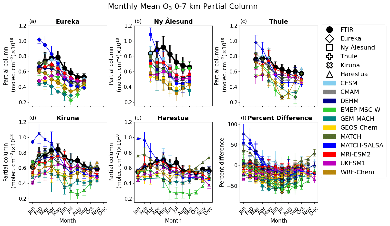
Figure 11 (a–e) Monthly mean FTIR (black) and smoothed model (colour) 0–7 km partial columns of O₃ (PC${}_{\mathrm{F},\mathrm{monthly},j}$ and PC${}_{\mathrm{M},\mathrm{monthly},j}$, respectively), for each location, shown with the same y axis. Error bars represent the standard deviation of the monthly mean. (f) Model–measurement mean percent difference by month (Δ_monthly,j) for each model (by colour) and location (by marker). Error bars represent standard deviation of the monthly mean percent difference.

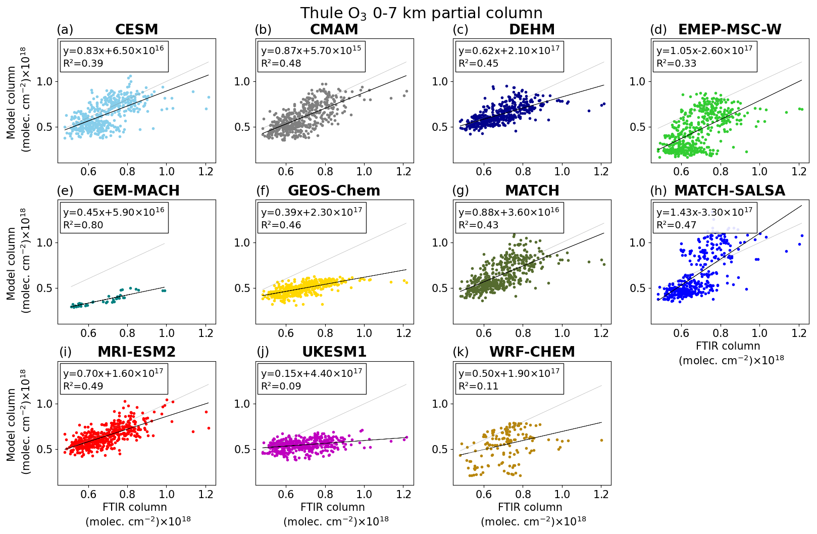
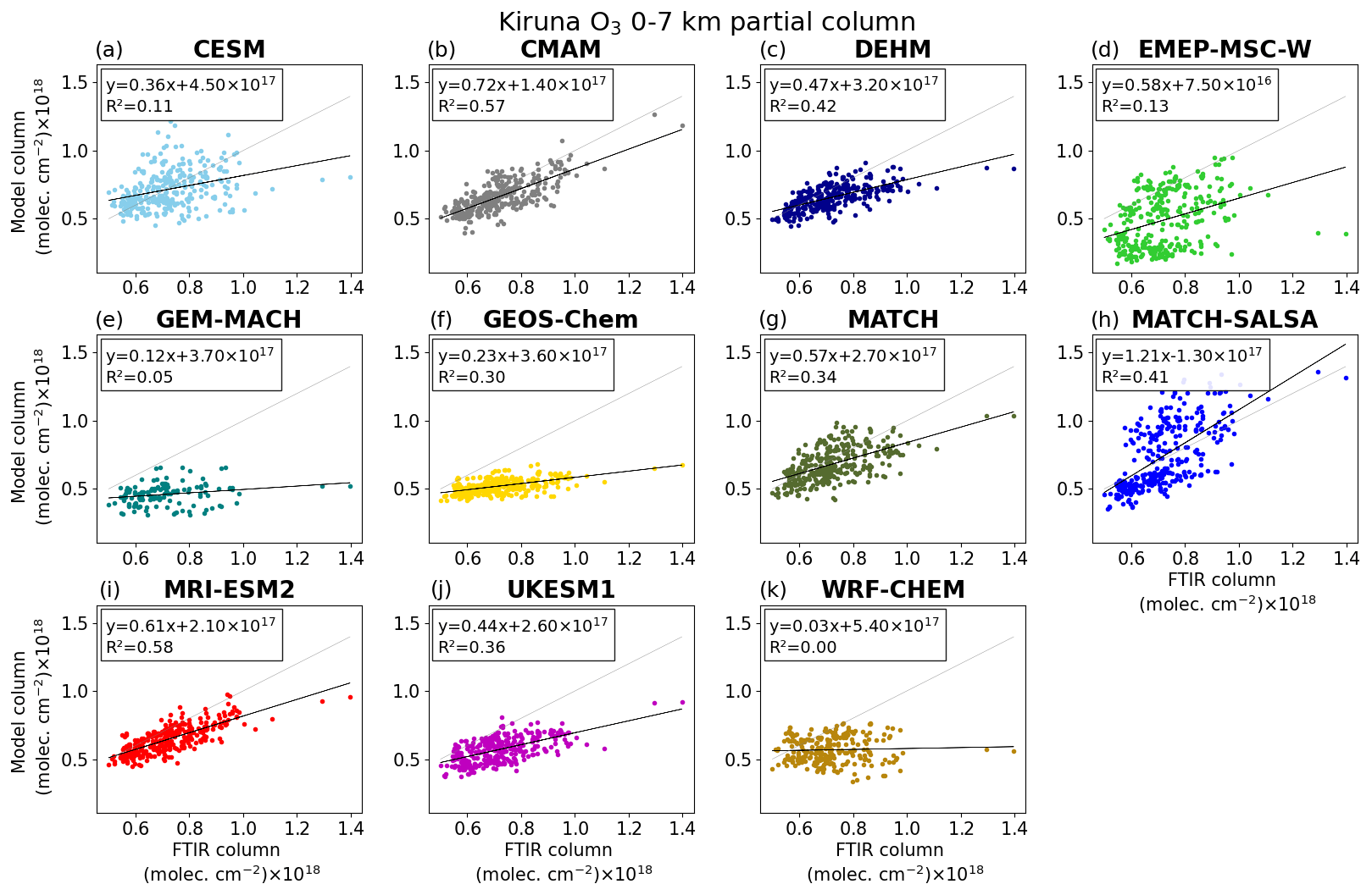
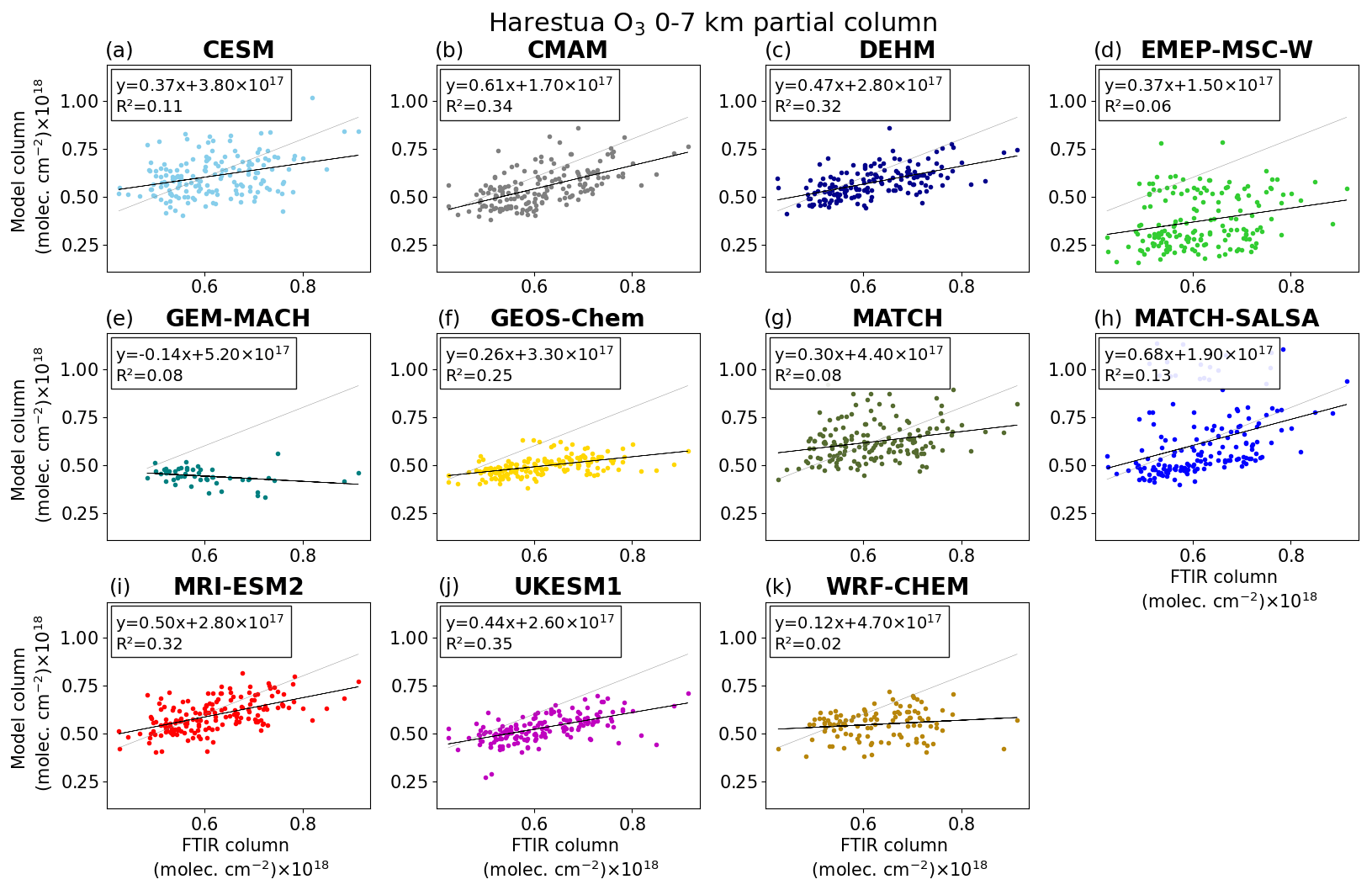
Figure 12 and Figs. C11–C14 show the model versus FTIR O₃ 0–7 km partial columns, with the line of best fit and R² shown in the legend, along with the 1:1 line. The general underprediction towards the largest values could be related to the underestimation in precursor species (such as CO or NO_x), a lack of long-range transport, an underestimation of ozone production in air masses during long-range transport to the Arctic, or a combination thereof. Using a MOZART-4 tagged tracer simulation of O₃, Wespes et al. (2012) examined source attributions of the tropospheric O₃ columns measured by the FTIR instruments at Thule and Eureka. Their analysis shows that the retrievals have a minimal contribution from the a priori profile (∼ 1 %), resulting in high vertical sensitivity throughout the troposphere. The tropospheric column source contributions were estimated, where over half was attributed to anthropogenic sources, followed by stratospheric influence and lastly lightning and biomass burning emissions (Wespes et al., 2012). The seasonal cycle of Arctic O₃ has been shown to vary based on geographical conditions, such as whether the site is coastal, inland, or at a high elevation (Whaley et al., 2023). Moreover, O₃ partial columns can be variable because they depend on the vertical distribution of O₃, which is determined by a combination of emissions, chemistry, dynamics, and radiation, all of which vary with altitude (Rap et al., 2015). Notably, Arctic O₃ columns have strong gradients in the influences on the vertical profile from mid-latitude regions (Europe, North America and Asia), which also vary with season (Monks et al., 2015). The combination of these factors leads to an increasingly complex series of model processes, which can also result in compounding errors. Without sensitivity simulations, like those carried out in Monks et al. (2015) and Rap et al. (2015), it is difficult to definitively say which of these processes are responsible for the underestimations found in this study.

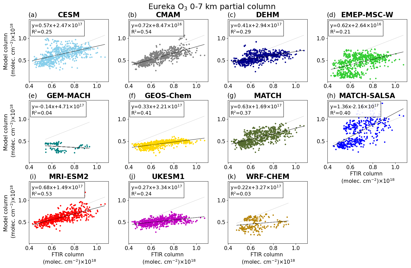
Figure 12 Smoothed model vs. FTIR 0–7 km partial columns of O₃ for Eureka, showing all available model–FTIR corresponding data. The black line is the line of best fit, where the equation and R² are noted in the legend. The 1:1 line is shown in light grey.

Figure 13 shows the summary of O₃ mean percent differences, R², and normalized root-mean-square error. The model–FTIR comparisons reveal that the spatial resolution, and inclusion of stratospheric chemistry in the models do not necessarily improve results (refer to Table 3 for horizontal resolution and stratospheric chemistry). For example, WRF-Chem, EMEP MSC-W, and GEM-MACH show a low R² and higher NRMSE (varying between sites and models), although contributing to this for WRF-Chem and GEM-MACH could be the limited number of analysis years (two and one, respectively). These air-quality focused models have detailed chemistry and were run at a higher spatial resolutions, whereas for example CMAM, a climate-focused model, has a coarser resolution with simplified tropospheric chemistry and demonstrates larger R² and smaller mean percent differences (Fig. 13). However, when considering the stratosphere, CMAM, which includes comprehensive stratospheric chemistry, has comparable metrics in Fig. 13 to DEHM, which uses prescribed climatologies for the stratosphere. Similarly, Whaley et al. (2022) stated that the degree of stratospheric chemistry in the models did not reveal a consistent benefit or handicap when comparing the models with surface measurements. Here, the O₃ partial column comparisons show significant variation, although again models largely underpredict FTIR measurements. The R², mean percent difference, and NRMSE are relatively consistent, where models with a larger percent difference also have weaker correlations and higher NRMSEs. An exception to this is CESM, which has one of the smallest overall differences across the models and locations. However, in the model vs. FTIR plot(s) (and Figs. 12, C11–C14), CESM has considerable scatter above and below the line of best fit, resulting in a decreased mean difference, while also reducing R², unlike MRI-ESM2, which has a similar mean percent difference and NRMSE but a stronger linear correlation.

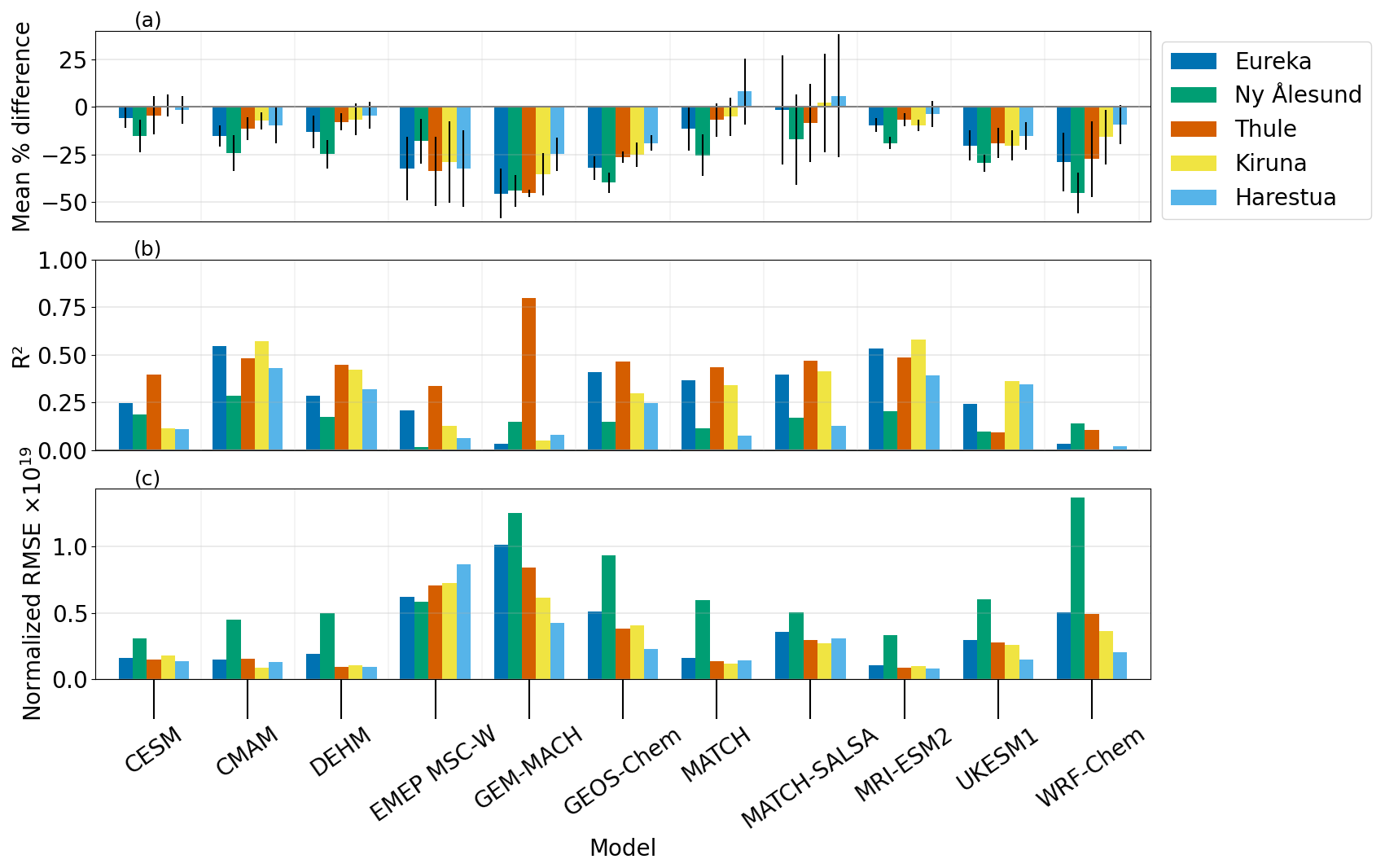
Figure 13 By model and location: (a) overall model–measurement mean percent difference for O₃ 0–7 km partial columns (Δ_O), with error bars that represent the standard deviation of the mean, as shown in the legend of Figs. C6–C10. (b) R² as shown in Figs. 12 and C11–C14. (c) Normalized root-mean-square error.

To supplement the aircraft and satellite campaigns undertaken for the POLARCAT study, daily mean O₃ measurements from the FTIR instruments at Eureka and Thule were compared to MOZART-4 simulations in Wespes et al. (2012). When examining a partial column from the ground to 300 hPa (approximately 9 km), the smoothed model showed a bias of −15 % relative to the FTIR. This is consistent with their analysis of aircraft observations, which revealed that the model underestimated O₃ by 5 %–15 %. Results here are similar to those presented in Wespes et al. (2012), where across all the locations and models, 24 of the 55 model–measurement mean percent differences were within ±15 % (see Fig. 15). The FTIR uncertainty for O₃ partial columns ranges from 3.9 % to 8.2%; the overall mean percent difference for MATCH-SALSA falls within these uncertainty bounds for all locations, and CESM, DEHM, MATCH, and MRI-ESM2 are within FTIR uncertainty for all locations but Ny Ålesund.

The AMAP SLCF assessment report finds that the multi-model mean of Arctic O₃ has a bias of +11 ± 3 % relative to surface measurements (AMAP, 2021). When partitioning results by region, all the models had positive biases when compared to the surface measurements in Alaska and negative biases in northern Europe, resulting in a relatively small mean bias across the Arctic as a whole (Whaley et al., 2022). Inaccuracies in long-range transport of O₃ and its precursors may have contributed to the increased discrepancy seen in the model–FTIR comparisons of the current study, particularly in partial columns with larger values. For example, the underestimation of CO may contribute to the negative bias in O₃ (see Figs. 9–10). Most models in AMAP (2021) show negative biases for Greenland and northern European locations, which would correspond closer geographically with the FTIR sites examined here. When comparing the AMAP models to TES (Tropospheric Emission Spectrometer) and ACE-FTS satellite O₃ measurements, the biases are negative at lower altitudes and become positive at higher altitudes (Whaley et al., 2022). AMAP model vs. ozonesonde comparisons showed similar elevated positive biases around 6–8 km of up to ±50 %, again indicating that the models may produce too much O₃ from mid-latitude anthropogenic emissions or that there may be too much downward transport of O₃ from the stratosphere (Whaley et al., 2023). The best performance in that study came from the multi-model mean, which simulated O₃ within ±8 % throughout the troposphere.

Figure 14 shows the monthly MMM for O₃ at all locations, along with the monthly mean FTIR and the associated percent difference. This shows that the models, as a whole, have an increased negative bias in the middle of the year relative to the winter, while still exhibiting a negative bias overall. The longitudinal range of sites examined here may limit biases to be negative, not capturing the positive–negative gradient from west–east in O₃ found in the AMAP report (AMAP, 2021; Whaley et al., 2022). Nonetheless, the model–FTIR O₃ comparisons reflect the proclivity of the models to underpredict Arctic O₃ in the lower troposphere, as also found in the aforementioned studies. The results of this study agree with results from previous studies and suggest that improvements are still needed for accurate modelling of O₃ and CO in the Arctic (Whaley et al., 2023). Models still require improvements in their treatment of stratosphere–troposphere exchange and Arctic boundary layer processes to better simulate Arctic O₃. Also required are better understanding and implementation of processes influencing O₃ removal through dry deposition and O₃ photochemical production from anthropogenic, biomass burning, and natural sources in the lower and middle troposphere.

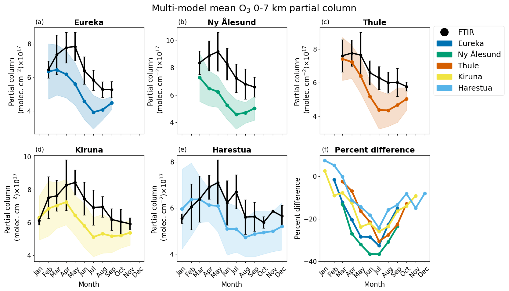
Figure 14 (a–e) Monthly mean FTIR (black) and multi-model mean (coloured) 0–7 km partial columns of O₃ (PC${}_{\mathrm{F},\mathrm{monthly},j}$ and PC${}_{\mathrm{MMM},\mathrm{monthly},j}$, respectively), with error bars and shaded areas representing the standard deviation of the mean. (f) Monthly mean percent difference in the MMM (Δ_O,MMM) for all locations.

5 Conclusions

This study compares atmospheric models with data from five Arctic NDACC ground-based FTIR spectrometers. The models simulate SLCFs and precursor gases with 3-hourly outputs for the years 2008, 2009, 2014, and 2015. Here, a total of 3 models are evaluated for CH₄, 9 for CO, and 11 for O₃. The model simulations are compared with FTIR tropospheric partial column measurements to assess performance throughout the year and across locations.

Generally, across the five locations, the model simulations of 0–7 km partial columns of CH₄, CO, and O₃ are underestimated. There were no significant patterns in the biases identified between the sites, species, or models examined. Modelled CH₄ partial columns are relatively consistent across the year, broadly capturing seasonal cycles, with the exception of a few outliers. CO simulations are inconsistent in reproducing the seasonal cycle, underpredicting springtime partial columns compared to the rest of the year, and skewing differences to be more positive when there are enhancements due to biomass burning events. Similarly, the models underestimated O₃ maxima more than O₃ minima in the troposphere. The multi-model means are reflective of these trends, for which (ignoring outliers) the CH₄ mean percent difference is relatively consistent across the year, CO has a maximum difference in the spring and a minimum in the summer, and O₃ has maximum difference centered around the summer. The AMAP SLCF assessment report found the best results using a multi-model mean for all species when comparing it with surface measurements (AMAP, 2021; Whaley et al., 2022). However, here, the multi-model means of the tropospheric column for all species are biased low. The average MMM mean difference is approximately −10 % for CH₄, −21 % for CO, and −18 % for O₃ (see Table 4), where the uncertainty in the FTIR 0–7 km partial column is on the order of 6 % on average. When examining the models and location pairs individually, the mean difference (inclusive of standard deviation) is within the respective FTIR uncertainty, for 6 of 15 model–FTIR comparisons for CH₄, 12 of 34 comparisons for CO, and 25 of 55 comparisons for O₃ (see Fig. 15).

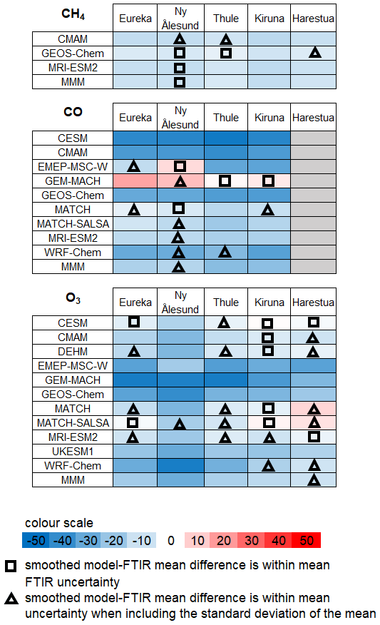
Figure 15 Summary of model–measurement mean percent difference (Δ_O) for each model and location by species. MMM is the multi-model mean (Δ_O,MMM). The colour scale indicates the mean percent difference relative to the FTIR measurements, from blue (−50 %) to red (+50 %). A square marker indicates that the mean percent difference is within the FTIR uncertainty. A triangle marker indicates that the mean difference is within the FTIR uncertainty combined with the standard deviation of the monthly mean percent difference.

These evaluations show that models are lacking some degree of transport and/or emissions to accurately reproduce tropospheric columns and seasonal variability in the Arctic. Model evaluation can provide a valuable checkpoint to help improve the representation of the Arctic in atmospheric models. NDACC FTIR spectrometers were selected for this project because of the wide range of species measured, high spectral resolution, multiple high-latitude sites, and publicly available data; in addition, the column-integrated FTIR measurements used in this study have a spatial and temporal footprint that is more representative of the free troposphere than in situ and satellite measurements. Future work would benefit from the inclusion of sensitivity studies, furthering the model–measurement comparisons with mid-latitude NDACC FTIR sites and extending comparisons to a longer time frame, with some models and locations having data from as early as 1990.

Appendix A: Additional figures for CH₄

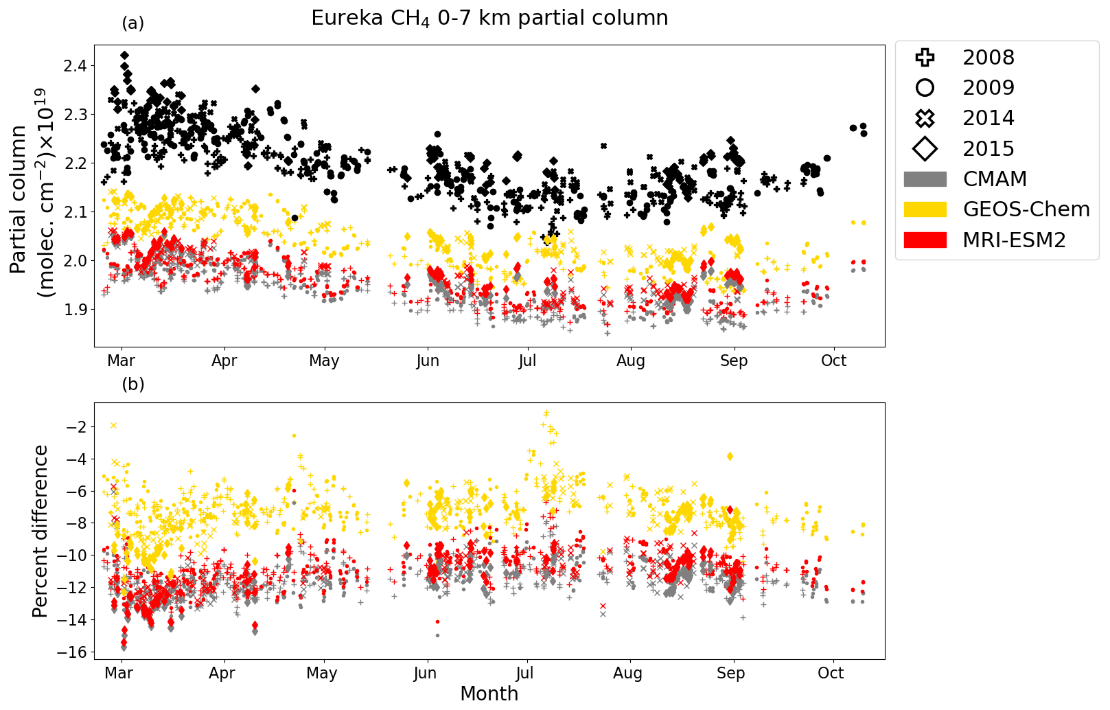
Figure A1 (a) FTIR (black) and smoothed model (colour) 0–7 km partial columns of CH₄ by day of year, from Eureka. Model data are the nearest in time to each FTIR measurement. (b) Model–measurement percent difference (Δ_i) from Eq. (2) by day of year. Each year is indicated by a different marker.

Figure A2 Same as Fig. A1 but for Ny Ålesund.

Figure A3 Same as Fig. A1 but for Thule.

Figure A4 Same as Fig. A1 but for Kiruna.

Figure A5 Same as Fig. A1 but for Harestua.

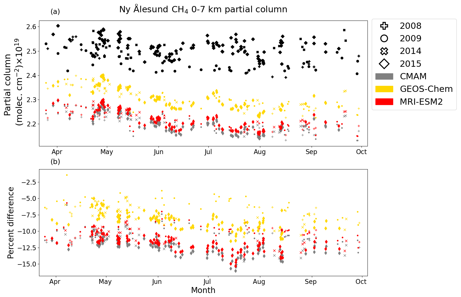
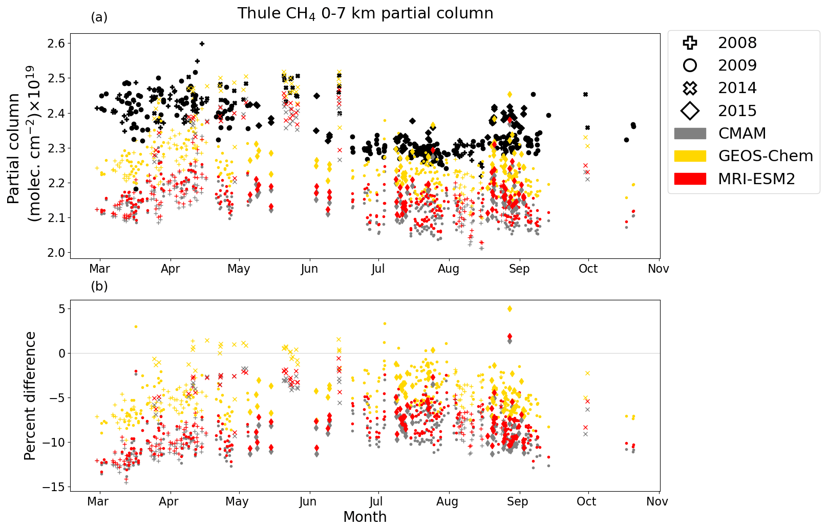
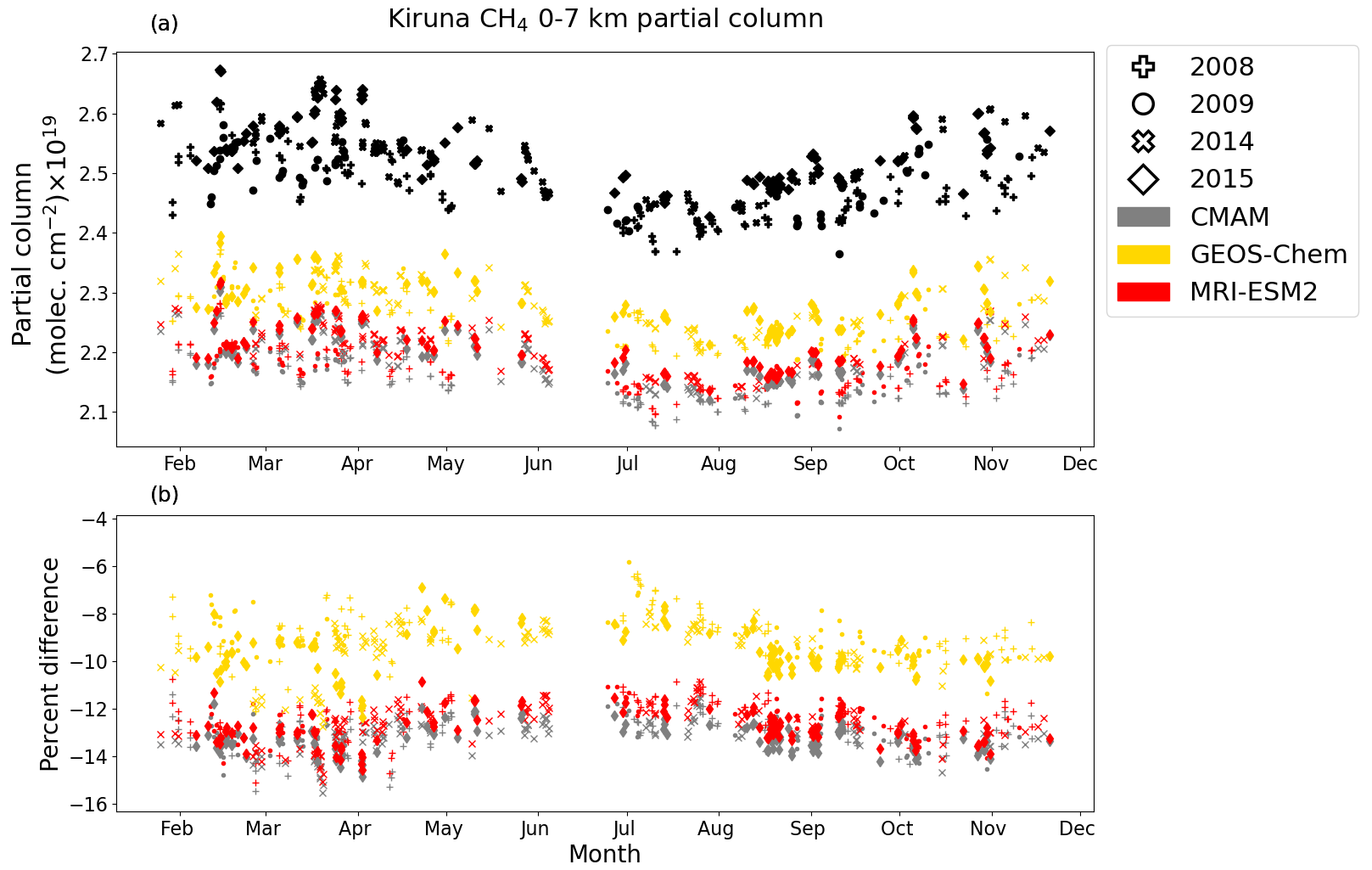
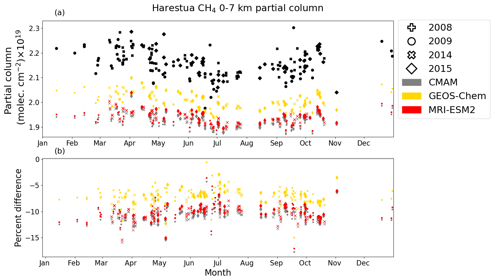
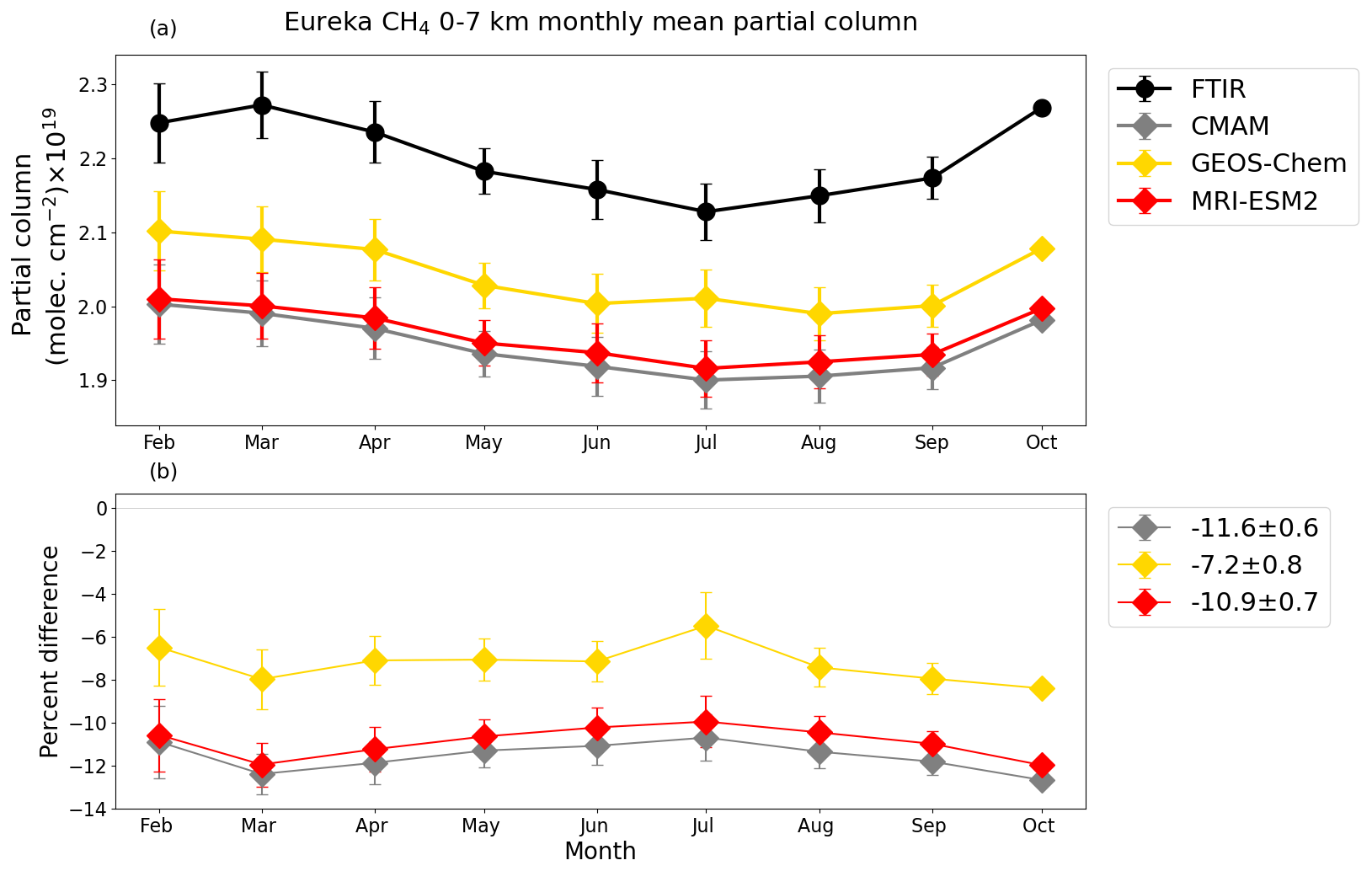
Figure A6 (a) Monthly mean FTIR (black) and smoothed model (colour) 0–7 km partial columns of CH₄ (PC${}_{\mathrm{F},\mathrm{monthly},j}$ and PC${}_{\mathrm{M},\mathrm{monthly},j}$, respectively), from Eureka using model data that are the nearest in time to each FTIR measurement shown in Fig. A1. Error bars represent the standard deviation of the monthly mean. (b) Model–measurement mean percent difference by month (Δ_monthly,j). Error bars represent standard deviation of the monthly mean percent difference. The legend in panel (b) shows the overall mean percent difference (Δ_O) with the standard deviation of the overall mean percent difference.

Figure A7 Same as Fig. A6 but for Ny Ålesund.

Figure A8 Same as Fig. A6 but for Thule.

Figure A9 Same as Fig. A6 but for Kiruna.

Figure A10 Same as Fig. A6 but for Harestua.

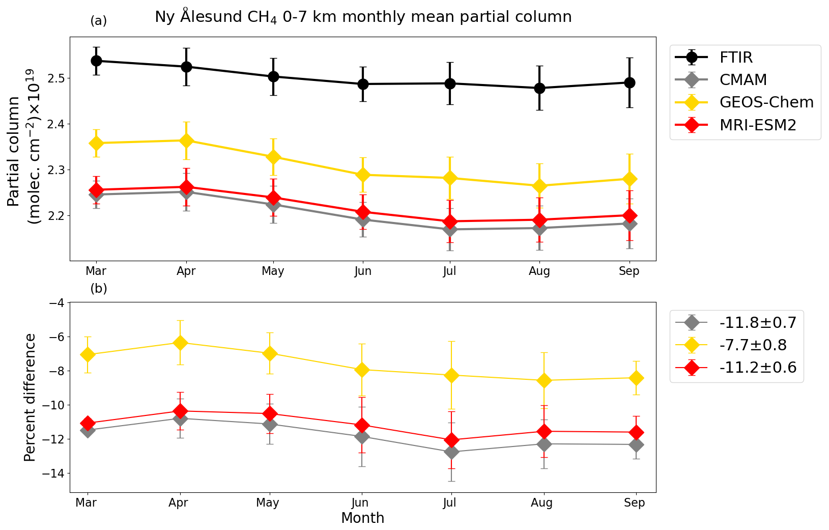
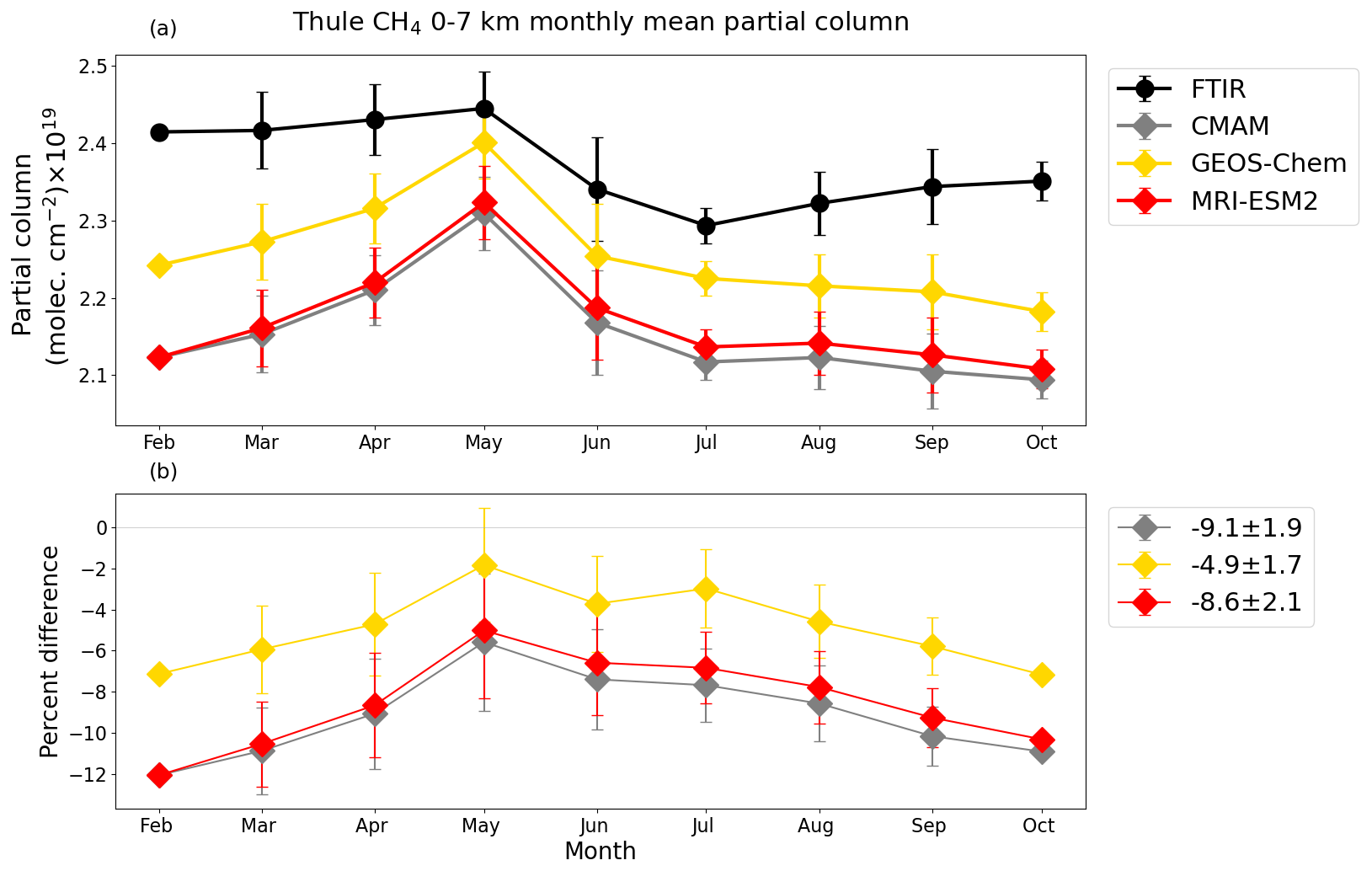
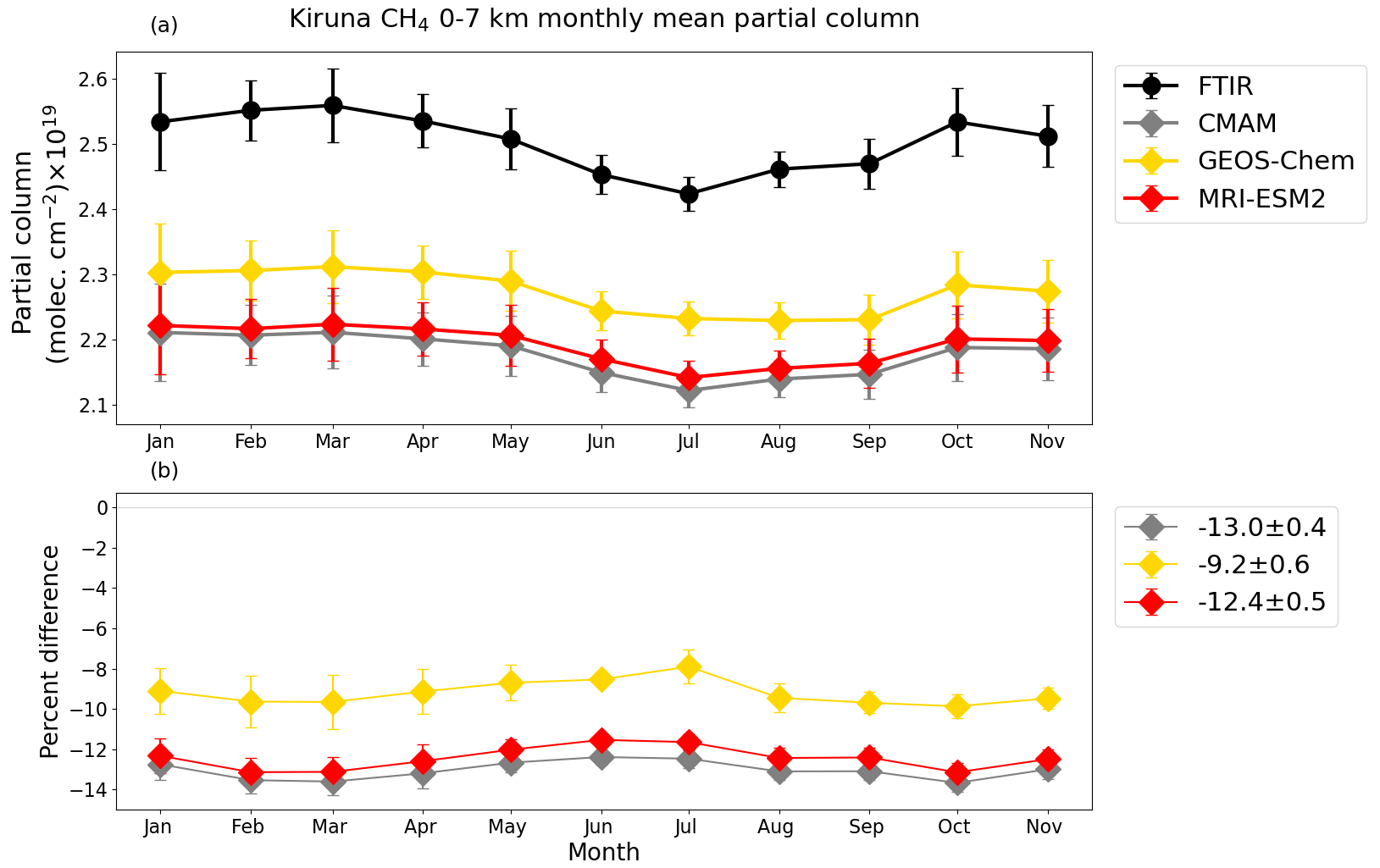
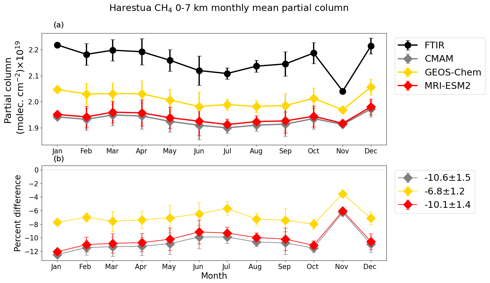
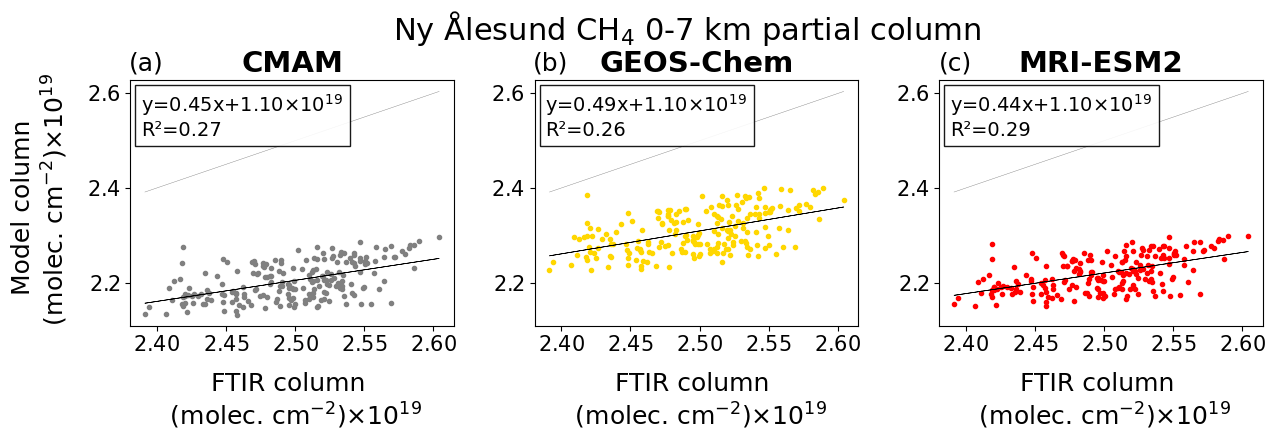
Figure A11 Smoothed model vs. FTIR 0–7 km partial column of CH₄ for Ny Ålesund, showing all available model–FTIR corresponding data. The black line is the line of best fit, where the equation and R² are noted in the legend. The 1:1 line is shown in light grey.

Figure A12 Same as Fig. A9 but for Thule.

Figure A13 Same as Fig. A9 but for Kiruna.

Figure A14 Same as Fig. A9 but for Harestua.

Appendix B: Additional figures for CO

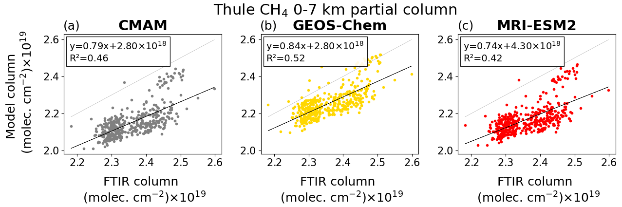
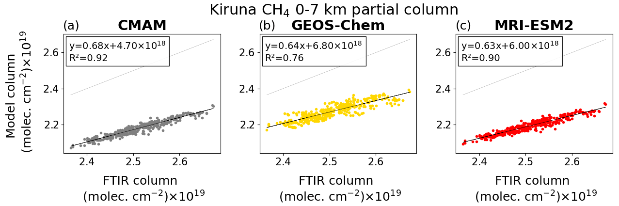
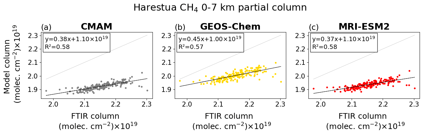
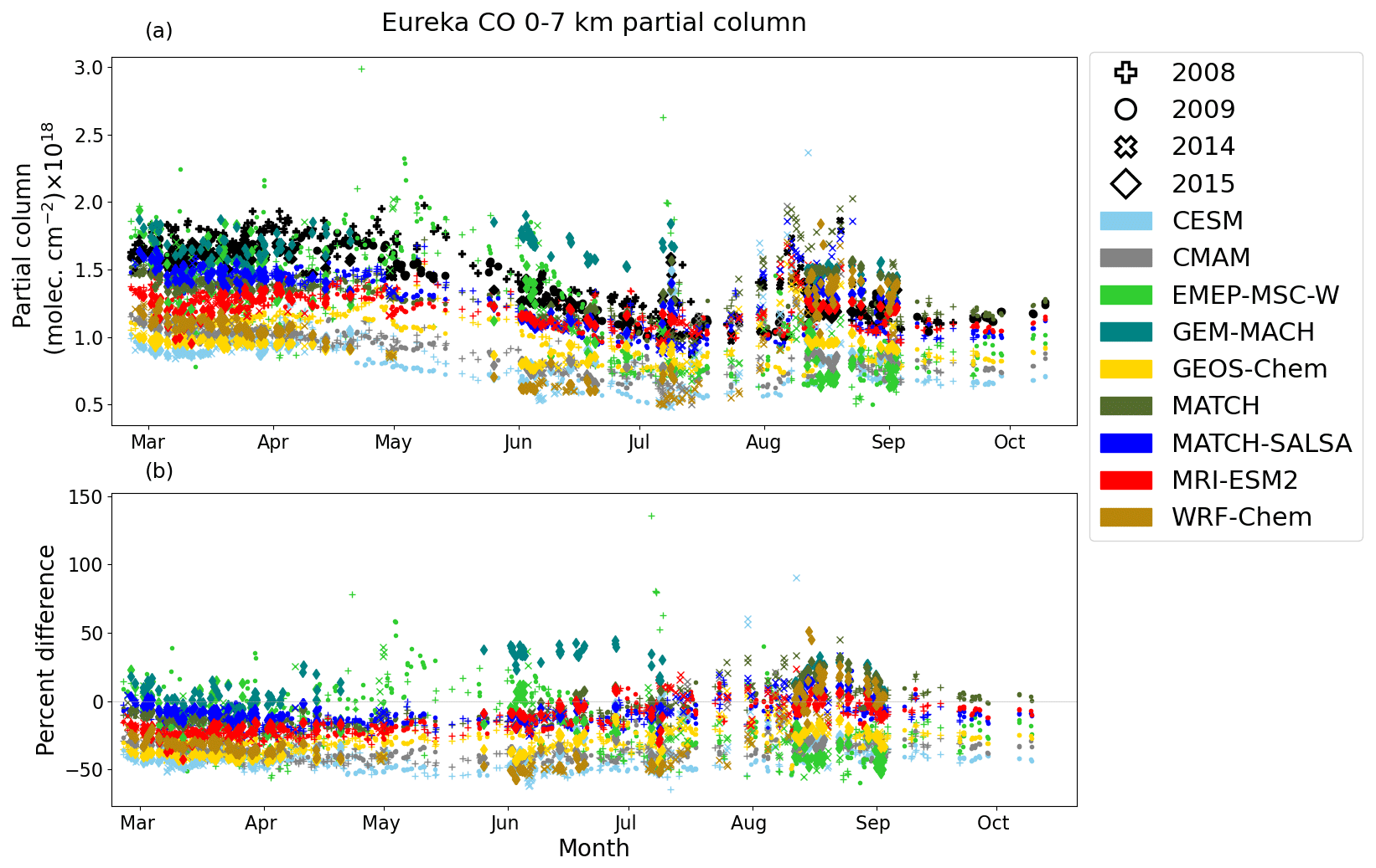
Figure B1 (a) FTIR (black) and smoothed model 0–7 km partial columns of CO by day of year, from Eureka. Model data are the nearest in time to each FTIR measurement. (b) Model–measurement percent difference (Δ_i) from Eq. (2) by day of year. Each year is indicated by a different marker.

Figure B2 Same as Fig. B1 but for Ny Ålesund.

Figure B3 Same as Fig. B1 but for Thule.

Figure B4 Same as Fig. B1 but for Kiruna.

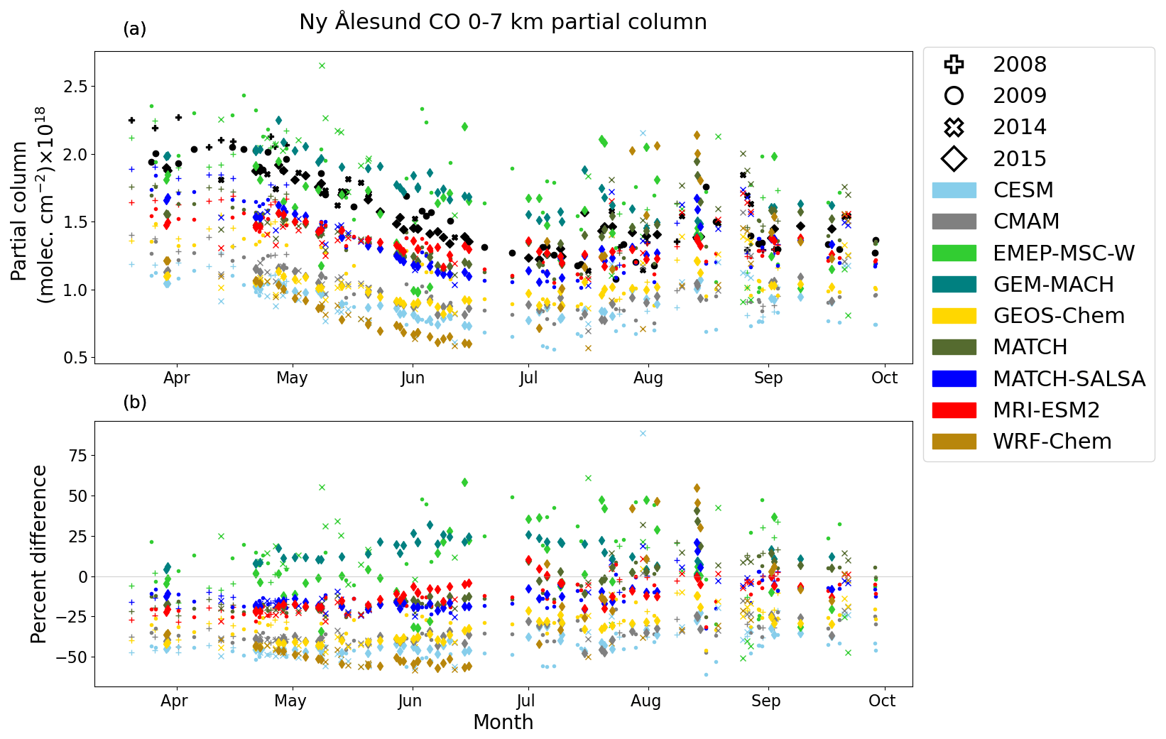
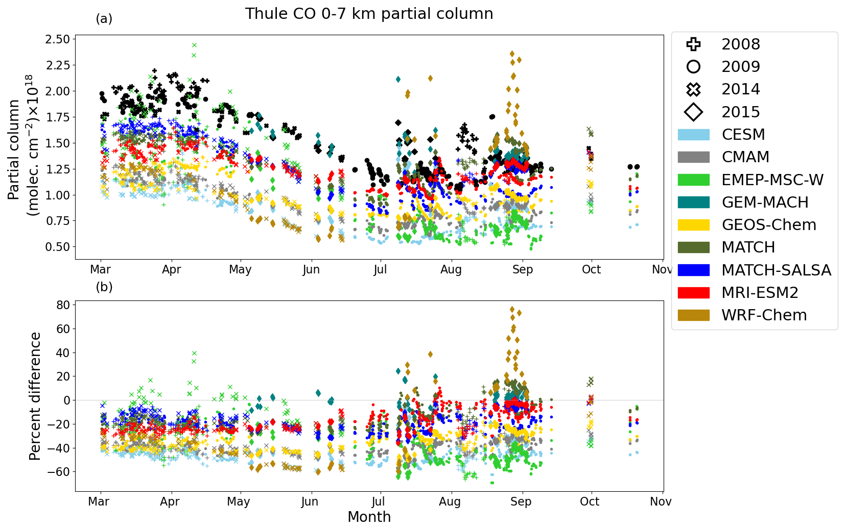
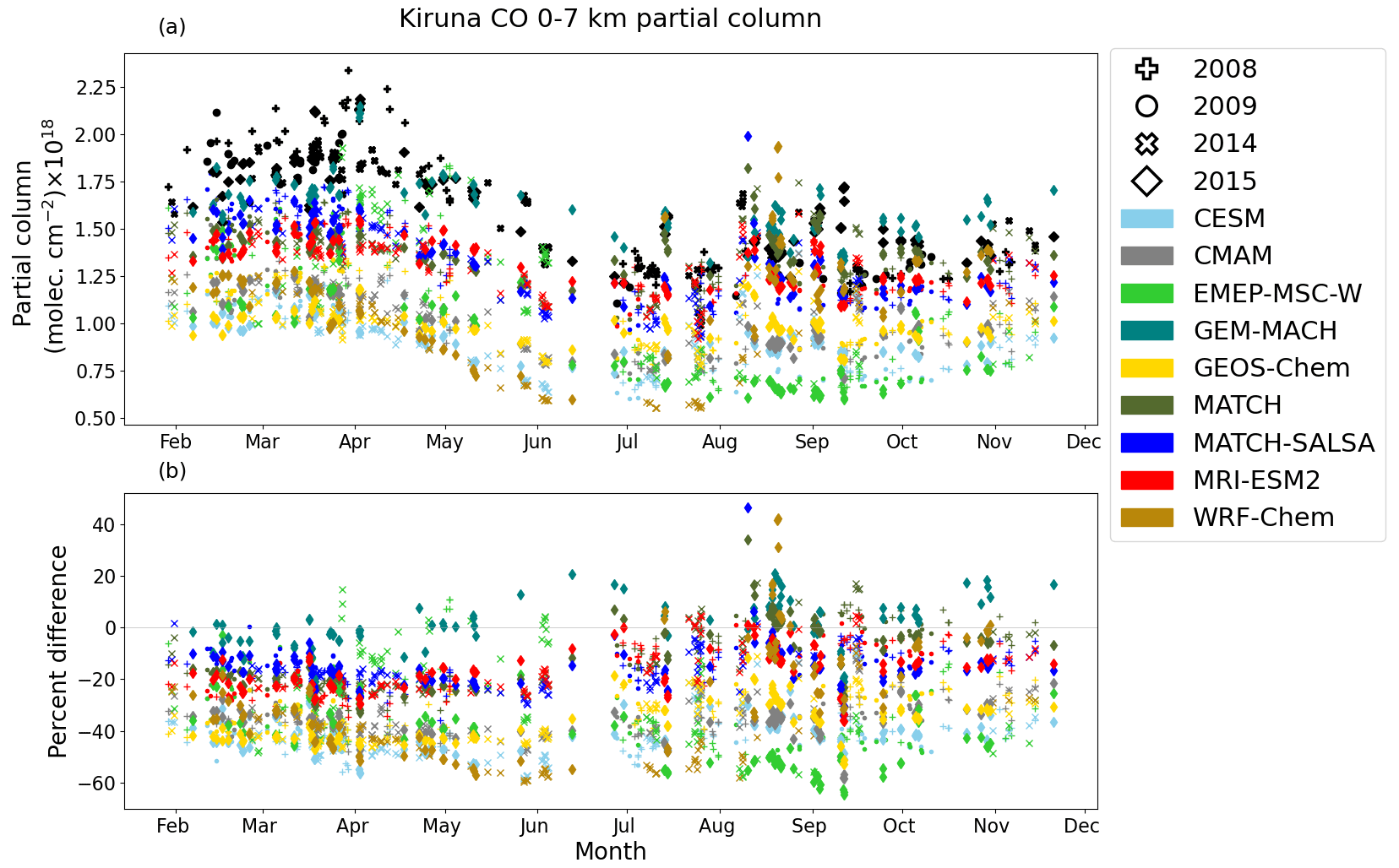
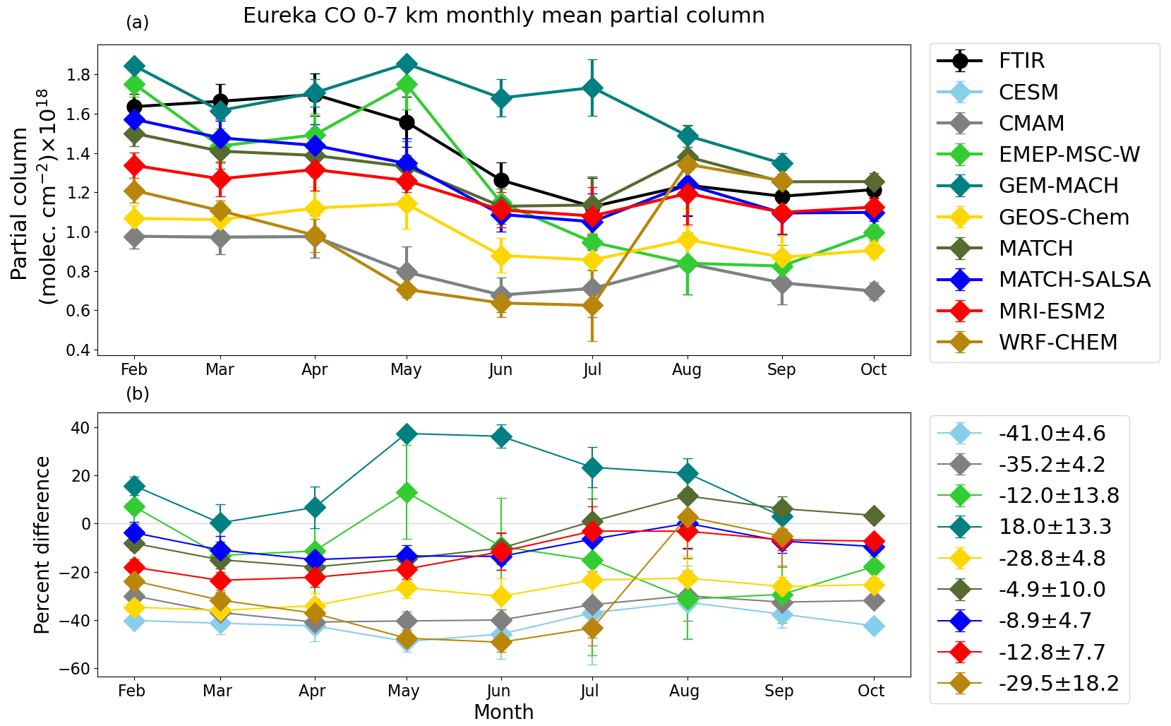
Figure B5 (a) Monthly mean FTIR (black) and smoothed model 0–7 km partial columns of CO (PC${}_{\mathrm{F},\mathrm{monthly},j}$ and PC${}_{\mathrm{M},\mathrm{monthly},j}$, respectively), from Eureka using model data that are the nearest in time to each FTIR measurement shown in Fig. B1. Error bars represent the standard deviation of the monthly mean. (b) Model–measurement mean percent difference by month (Δ_monthly,j). Error bars represent standard deviation of the monthly mean percent difference. The legend in panel (b) shows the overall mean percent difference (Δ_O) with the standard deviation of the overall mean percent difference.

Figure B6 Same as Fig. B5 but for Ny Ålesund.

Figure B7 Same as Fig. B5 but for Thule.

Figure B8 Same as Fig. B5 but for Kiruna.

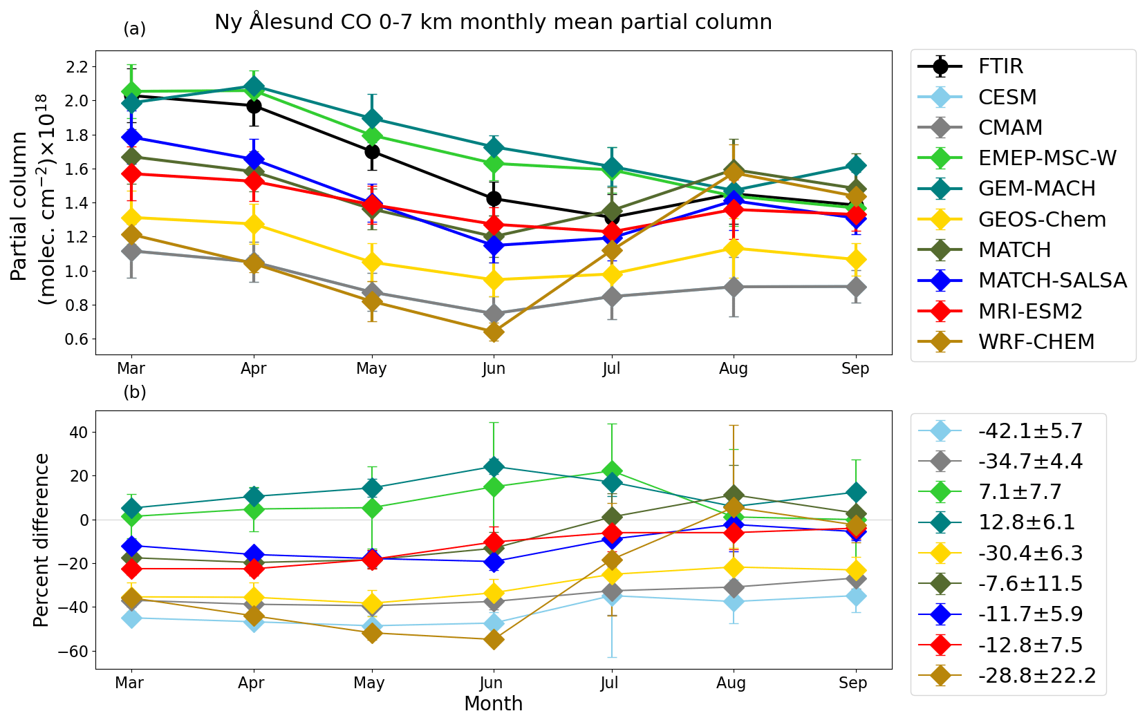
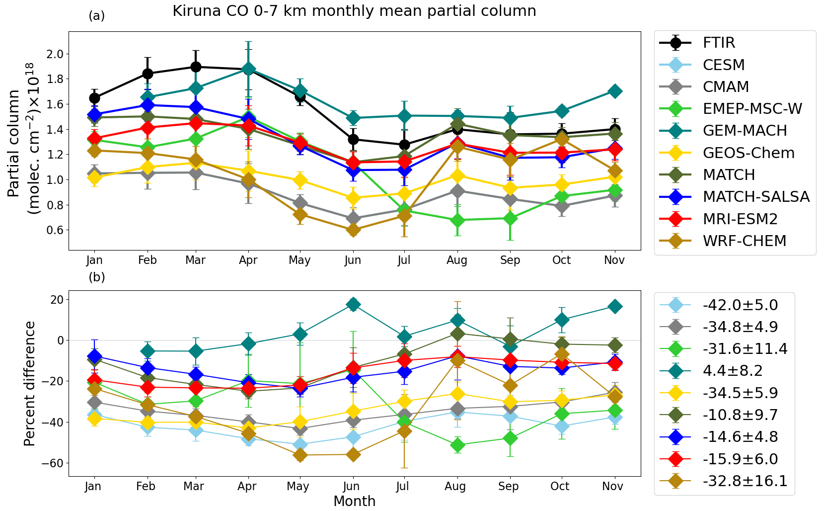
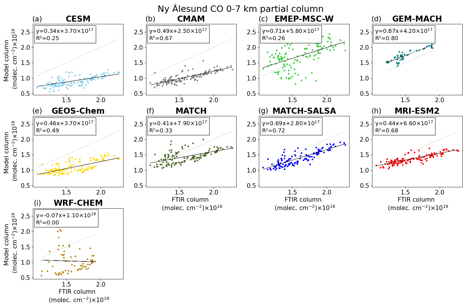
Figure B9 Smoothed model vs. FTIR 0–7 km partial columns of CO for Ny Ålesund, showing all available model–FTIR corresponding data. The black line is the line of best fit, where the equation and R² are noted in the legend. The 1:1 line is shown in light grey.

Figure B10 Same as Fig. B9 but for Thule.

Figure B11 Same as Fig. B9 but for Kiruna.

Appendix C: Additional figures for O₃

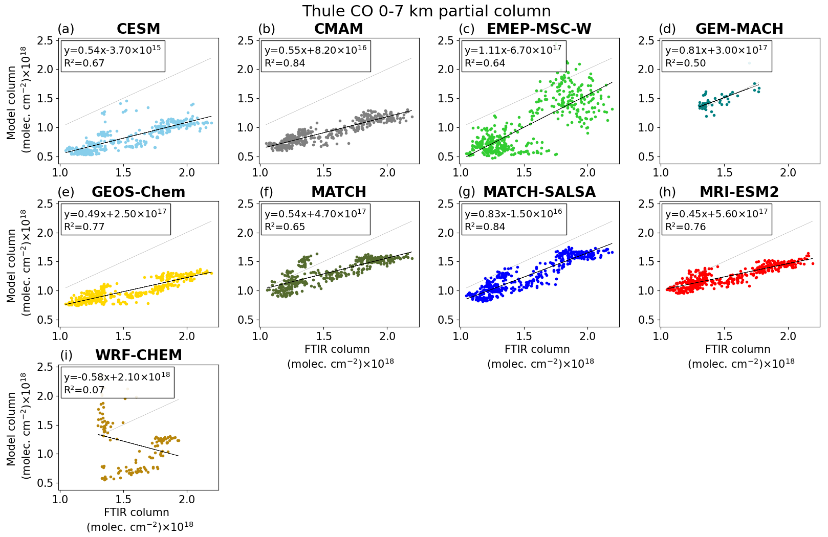
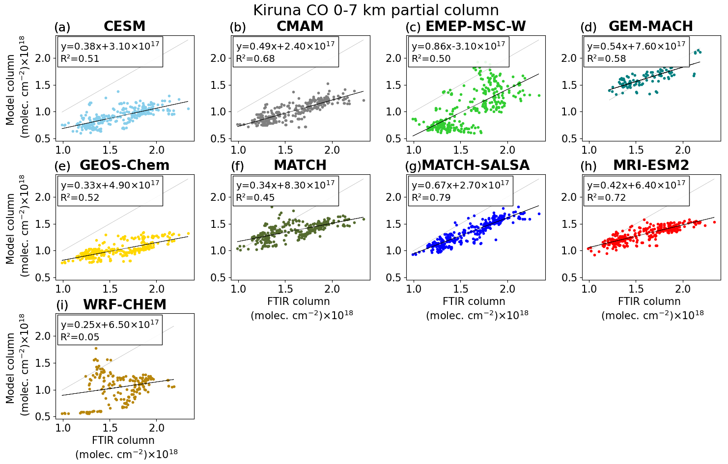
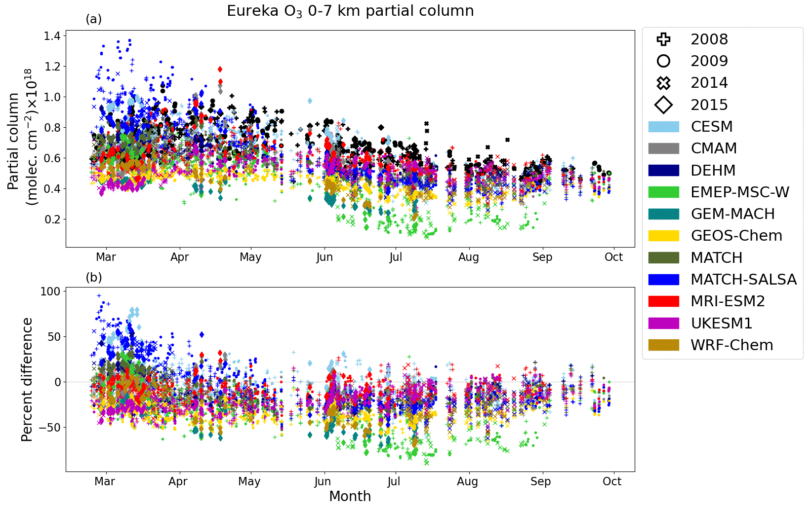
Figure C1 (a) FTIR (black) and smoothed model partial columns of O₃ by day of year, from Eureka. Model data are the nearest in time to each FTIR measurement. (b) Model–measurement percent difference (Δ_i) from Eq. (2) by day of year. Each year is indicated by a different marker.

Figure C2 Same as Fig. C1 but for Ny Ålesund.

Figure C3 Same as Fig. C1 but for Thule.

Figure C4 Same as Fig. C1 but for Kiruna.

Figure C5 Same as Fig. C1 but for Harestua.

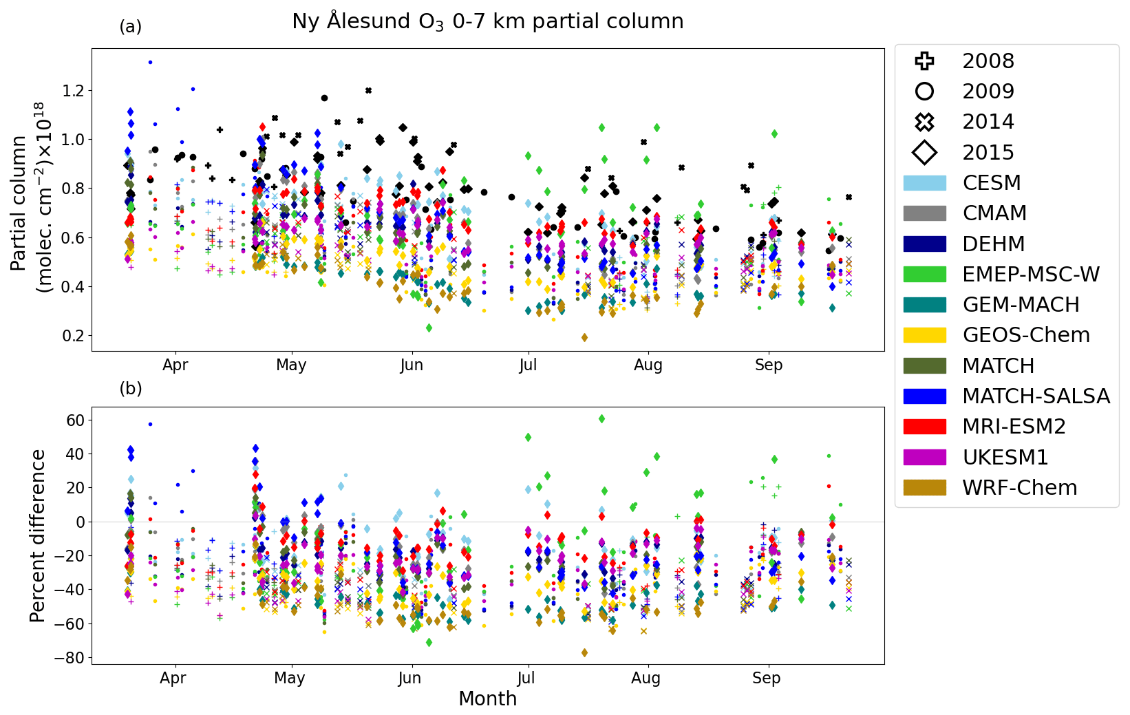
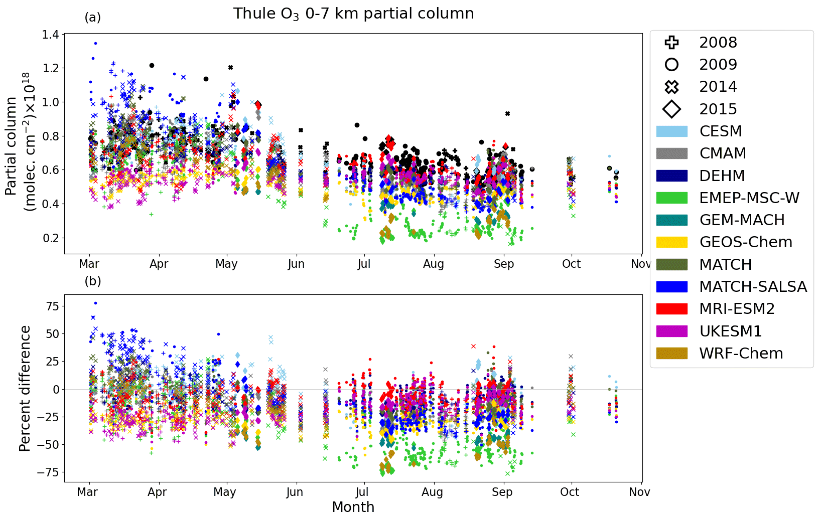
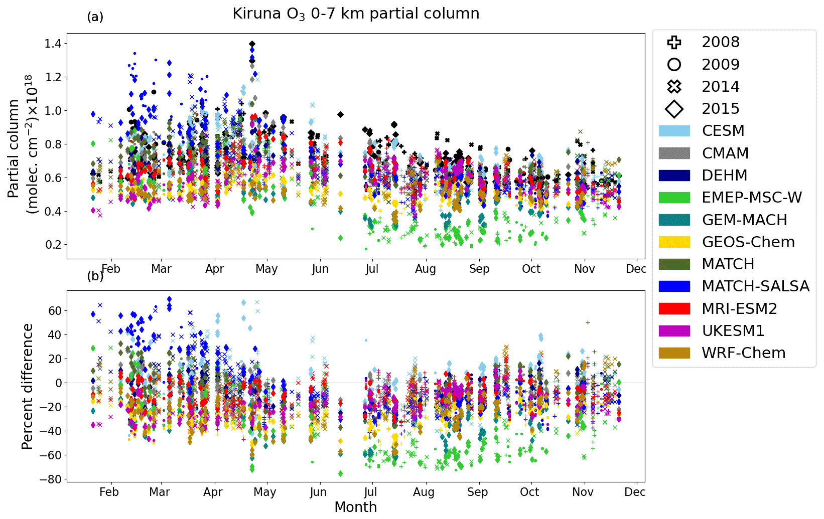
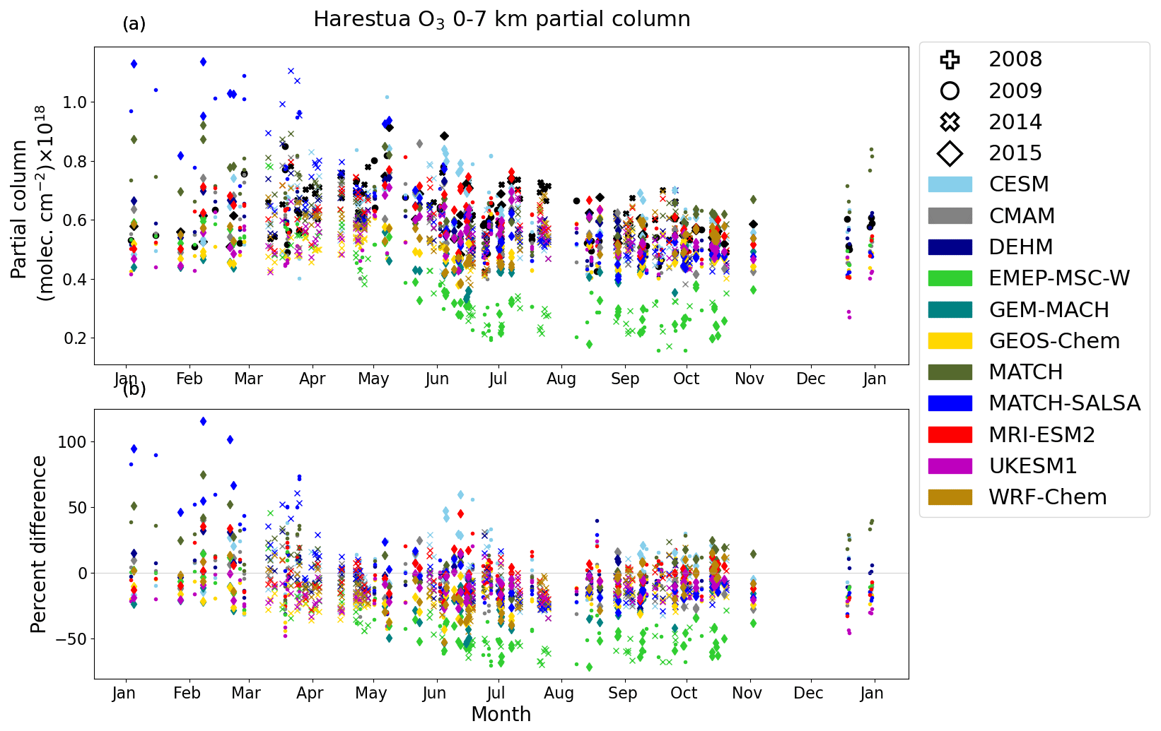
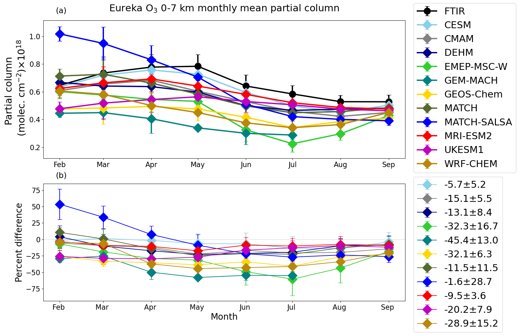
Figure C6 (a) Monthly mean FTIR (black) and smoothed model 0–7 km partial columns of O₃ (PC${}_{\mathrm{F},\mathrm{monthly},j}$ and PC${}_{\mathrm{M},\mathrm{monthly},j}$, respectively) from Eureka using model data that are the nearest in time to each FTIR measurement shown in Fig. C1. Error bars represent the standard deviation of the monthly mean. (b) Model–measurement mean percent difference by month (Δ_monthly,j). Error bars represent standard deviation of the monthly mean percent difference. The legend in panel (b) shows the overall mean percent difference (Δ_O) with the standard deviation of the overall mean percent difference.

Figure C7 Same as Fig. C6 but for Ny Ålesund.

Figure C8 Same as Fig. C6 but for Thule.

Figure C9 Same as Fig. C6 but for Kiruna.

Figure C10 Same as Fig. C6 but for Harestua.

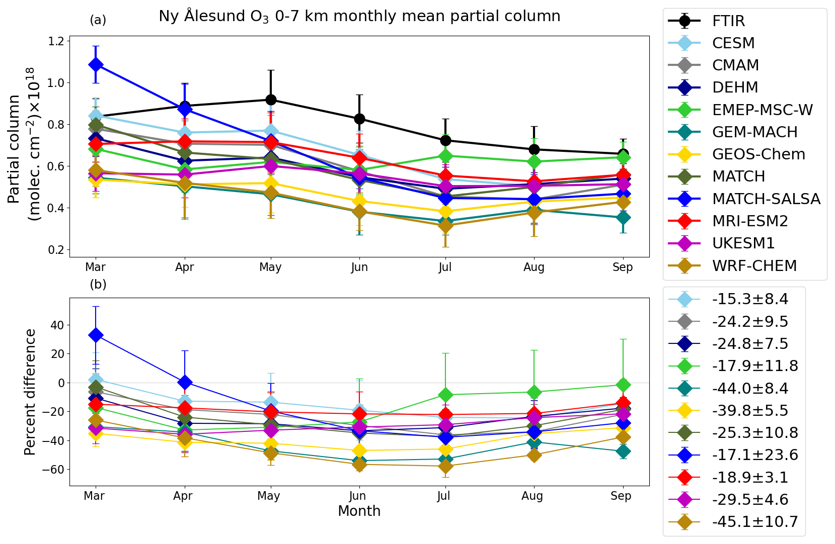
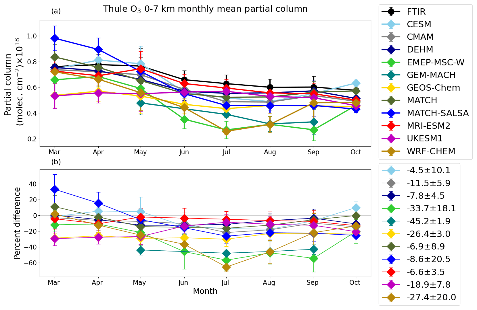
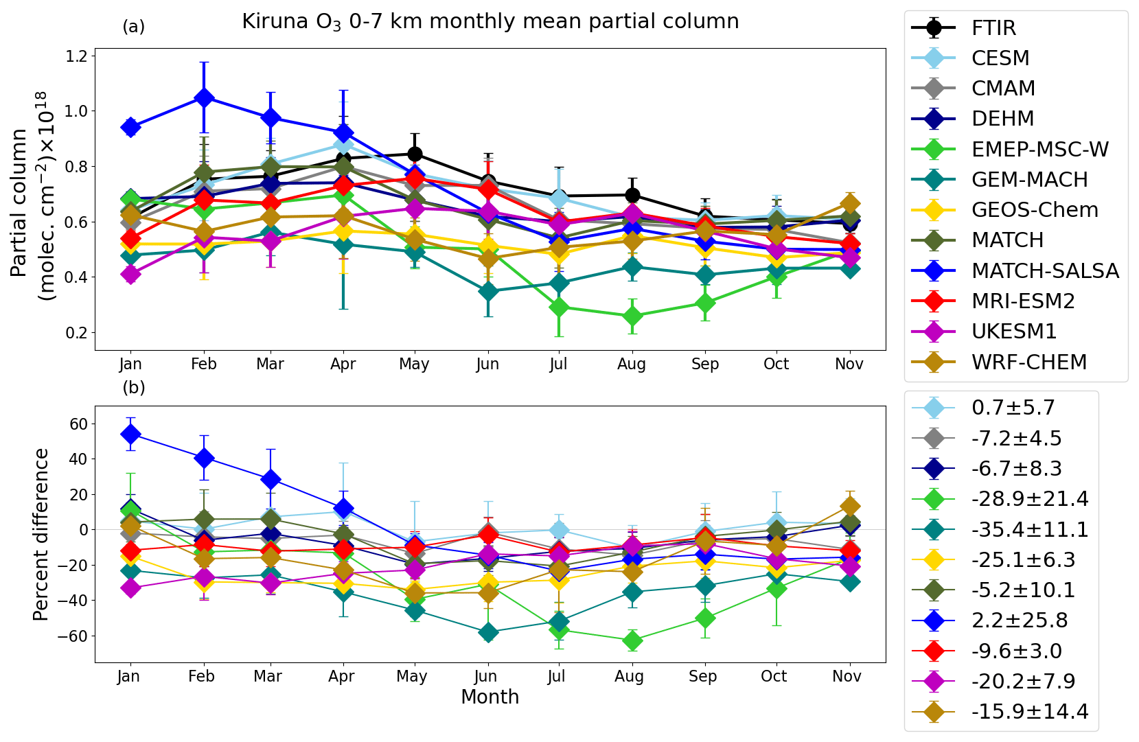
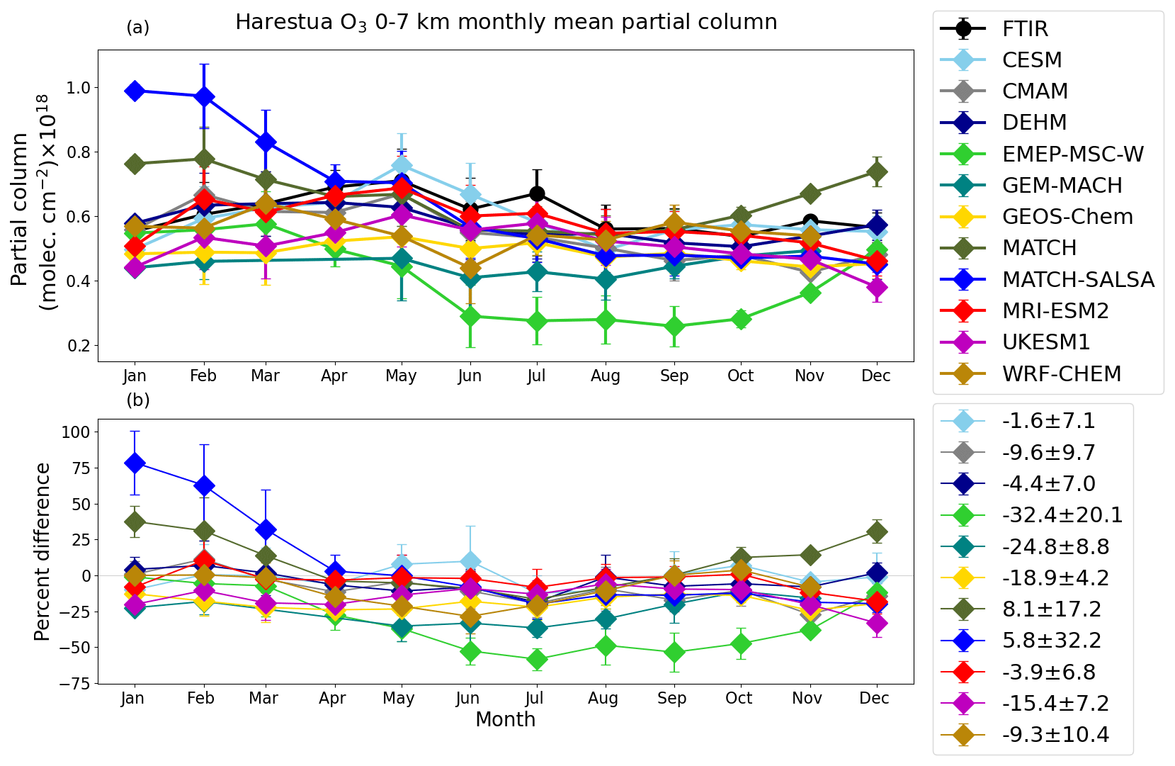
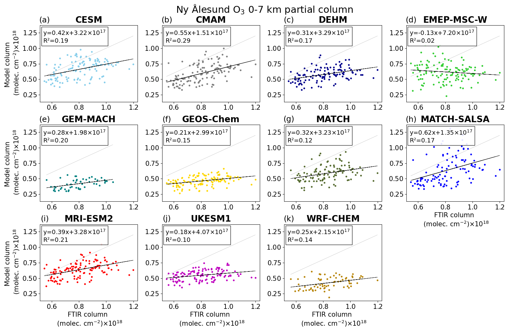
Figure C11 Model vs. FTIR 0–7 km partial columns of O₃ for Ny Ålesund, showing all available model–FTIR corresponding data. The black line is the line of best fit, where the equation and R² are noted in the legend. The 1:1 line is shown in light grey.

Figure C12 Same as Fig. C11 but for Thule.

Figure C13 Same as Fig. C11 but for Kiruna.

Figure C14 Same as Fig. C11 but for Harestua.