Verifying national inventory-based combustion emissions of CO₂ across the UK and mainland Europe using satellite observations of atmospheric CO and CO₂

Under the Paris Agreement, countries report their anthropogenic greenhouse gas emissions in national inventories, which are used to track progress towards mitigation goals, but they must be independently verified. Atmospheric observations of CO₂, interpreted using inverse methods, can potentially provide that verification. Conventional CO₂ inverse methods infer natural CO₂ fluxes by subtracting a priori estimates of fuel combustion from the a posteriori net CO₂ fluxes, assuming that a priori knowledge for combustion emissions is better than for natural fluxes. We describe an inverse method that uses measurements of CO₂ and carbon monoxide (CO), a trace gas that is co-emitted with CO₂ during combustion, to report self-consistent combustion emissions and natural fluxes of CO₂. We use an ensemble Kalman filter and the GEOS-Chem atmospheric transport model to explore how satellite observations of CO and CO₂ collected by the TROPOspheric Monitoring Instrument (TROPOMI) and Orbiting Carbon Observatory-2 (OCO-2), respectively, can improve understanding of combustion emissions and natural CO₂ fluxes across the UK and mainland Europe in 2018–2021. We assess the value of using satellite observations of CO₂, with and without CO, above what is already available from the in situ network. Using CO₂ satellite observations leads to small corrections to a priori emissions that are inconsistent with in situ observations, due partly to the insensitivity of the atmospheric CO₂ column to CO₂ emission changes. When we introduce satellite CO observations, we find better agreement with our in situ inversion and a better model fit to atmospheric CO₂ observations. Our regional mean a posteriori combustion CO₂ emission ranges from 4.6–5.0 Gt a⁻¹ (1.5 %–2.4 % relative standard deviation), with all inversions reporting an overestimate for Germany's wintertime emissions. Our national a posteriori CO₂ combustion emissions are highly dependent on the assumed relationship between CO₂ and CO uncertainties, as expected. Generally, we find better results when we use grid-scale-based a priori CO₂:CO uncertainty estimates rather than a fixed relationship between the two species.

1 Introduction

More than 40 % of the cumulative net CO₂ emissions from 1850 to 2019 have occurred since 1990, resulting in a global mean surface temperature rise of 0.45 °C (IPCC, 2022). If the 2019 emission rate continues to 2030, we will have exhausted the remaining carbon budget to keep global mean temperatures within 1.5 °C and depleted a third of the remaining carbon budget for 2 °C (IPCC, 2022). These estimates assume that the land biosphere and ocean will continue to respond to changes in climate as they do today. The most effective lever at our disposal to rapidly reduce atmospheric concentrations of CO₂ is a commensurately large, rapid, and targeted reduction in emissions, as recognized by the Paris Agreement. A clearer understanding of the national importance of individual CO₂ emitting sectors is needed to develop effective emission mitigation policies. Similarly, global to regional observing networks are needed to verify the effectiveness of these policies to reduce national emissions from individual sectors. Here, we focus on the potential of satellite observations to verify changes in combustion emissions of CO₂ across the UK and mainland Europe.

Under the Paris Agreement, countries annually report estimates of their anthropogenic greenhouse gas emissions in national inventories, typically with a lag of more than 12 months, as an approach to establish and track progress towards emission mitigation goals. These inventory-based estimates use bottom-up methods that typically rely on national activity data (e.g. power plant fuel consumption) and country-specific emission factors (e.g. CO₂ emissions per unit of fuel consumed); the corresponding emission uncertainties are related to the underlying datasets and methodologies. To set effective national emission mitigation targets and track progress, it is important to estimate CO₂ combustion emissions accurately in these inventories, including accurate estimates of their uncertainties.

Observations of atmospheric CO₂ provide an independent evaluation of reported bottom-up CO₂ flux estimates (e.g. Peylin et al., 2013). A top-down approach uses these atmospheric measurements to infer the most likely a posteriori distribution of CO₂ fluxes that would explain the observations, accounting for uncertainties associated with the measurements of the method. An atmospheric transport model is used to relate the gridded a priori estimates of CO₂ fluxes to 4-D distributions of atmospheric CO₂ concentrations. An observation operator is then applied to this 4-D distribution, which describes how a particular instrument samples the atmosphere at a given time and place. The resulting model atmospheric CO₂ measurements are then confronted with the observations, and the a priori flux estimates are adjusted to minimize any model–observation differences, resulting in a posteriori flux estimates that are consistent with a priori and measurement information. Ground-based in situ observations from the pan-European measurement network have been used extensively to estimate regional net CO₂ fluxes (e.g. Scholze et al., 2019; Ramonet et al., 2020; Rödenbeck et al., 2020; Thompson et al., 2020).

Separating the combustion and natural components of the net a posteriori CO₂ flux estimates is non-trivial, which has resulted in a range of approaches being developed by researchers (e.g. Konovalov et al., 2016; Boschetti et al., 2018; Yang et al., 2023; Feng et al., 2024). The most common approach is to assume we have near-perfect knowledge of anthropogenic emissions, subtract these a priori emission estimates from the net a posteriori values, and then interpret the residual as fluxes from the natural biosphere to compare with inventory estimates (e.g. White et al., 2019; Deng et al., 2022). The spatial and temporal information on both emissions and uncertainties is often highly uncertain but also needed to interpret atmospheric measurements (Super et al., 2020; Oda et al., 2023). There is also now a greater focus on estimating changes in anthropogenic emissions, as countries introduce policies to decarbonize their economies.

With this impetus in mind, there is an urgent need to develop and evaluate robust methods that separate the combustion and natural influences on changes in atmospheric CO₂ at city scale (e.g. Silva et al., 2013; Reuter et al., 2019; Goldberg et al., 2019; Yang et al., 2023) and national scale (Palmer et al., 2006) using additional observations of trace gases co-emitted during the combustion process, e.g. CO and NO₂. Previous work has focused on using ground-based or aircraft in situ measurements of CO₂ and co-emitted trace gases (see references above), but we need to understand how we best use satellite observations to estimate anthropogenic emissions of CO₂, particularly in the context of the billion-euro investment in the Copernicus CO₂ Monitoring Mission, CO2M (Sierk et al., 2021).

Observations of atmospheric CO₂ collected by satellites have the advantage of global spatial coverage, subject to cloud cover, and have been used to constrain CO₂ flux estimates on the spatial scale of thousands of kilometres (e.g. Chevallier et al., 2014, 2019; Feng et al., 2017; Palmer et al., 2019; Byrne et al., 2023). To date, few studies have focused on using these data to constrain CO₂ flux estimates over mainland Europe or the UK because there is less information about surface CO₂ on those spatial scales from the current generation of CO₂ satellites (OCO-2 and GOSAT) than the in situ measurement networks. This is in part because satellite observations of the atmospheric column of CO₂ are less sensitive to CO₂ surface fluxes compared to in situ measurement networks. It is widely anticipated that the significant increase in the volume and spatial coverage of data collected by CO2M will dramatically increase the competitiveness of satellite observations for estimating national-scale emissions across mainland Europe and the UK. CO2M will focus on quantifying anthropogenic emissions of CO₂ and methane and will form part of the European measurement and verification support capacity (Janssens-Maenhout et al., 2020). It will likely consist of three satellites, each with a push-broom imaging spectrometer that has an across-track swath of ∼250 km with a spatial resolution of 4 km² (Sierk et al., 2021).

In this study, we quantify the ability of current satellite observations of CO₂ and CO to constrain country-scale combustion and non-combustion CO₂ flux estimates across the UK and mainland Europe. We use atmospheric CO₂ observations from the NASA OCO-2 instrument and CO observations from the ESA TROPOspheric Monitoring Instrument (TROPOMI) to estimate monthly CO₂ fluxes for 2018–2021. Our work is part of a larger effort to develop rigorous methods to evaluate nationally reported CO₂ emissions using in situ and satellite observations. In the next section, we describe the methods we use to infer simultaneously combustion and natural fluxes of CO₂ using OCO-2 and TROPOMI data. Section 3 describes our results. We conclude the paper in Sect. 4.

2 Data and methods

Here, we describe the measurements we use to infer CO₂ fluxes across the UK and mainland Europe; the GEOS-Chem atmospheric chemistry transport model that describes the relationship between a priori inventories, atmospheric chemistry and transport, and the observed atmospheric concentrations of CO₂; and the ensemble Kalman filter that is used to infer CO₂ fluxes from a priori knowledge and the measurements. We describe the results from three inversions. For the first inversion we independently estimate a posteriori emissions of CO and CO₂. For the second and third inversions we assume combustion CO and CO₂ emission errors are correlated and report jointly estimated a posteriori CO and CO₂ fluxes. For the second inversion we assume a perfect correlation between these emissions errors and for the third inversion we use emission error correlations that are determined from sector-based errors in the bottom-up emission inventory (Super et al., 2024).

2.1 Satellite and in situ observations

For CO₂, we use observations of the atmospheric CO₂ column-averaged dry-air mole fraction (XCO₂) from the OCO-2 satellite, launched in 2014 (Crisp et al., 2017; Eldering et al., 2017). We use OCO-2 ACOS v10r data for 2018–2021 (OCO-2 Science Team et al., 2020a; Taylor et al., 2023). For CO, we use XCO observations from TROPOMI, July 2018–December 2021, aboard the Sentinel-5P satellite, launched in 2017 (Veefkind et al., 2012; for CO retrieval: Vidot et al., 2012; Landgraf et al., 2016). For both satellite products, we filter observations as recommended in the product user guide, including a strict quality assurance flag value of >0.75 for TROPOMI XCO. We remove glint observations and those over the oceans and collate satellite columns and averaging kernels to a 0.25°×0.3125° spatial grid to match model output (Fig. 1). To compare our model output to the satellite observations, we first sampled the model at the overpass time and location of each instrument. We then interpolate our model pressure levels to the satellitepressure levels and apply the scene-dependent retrieval averaging kernel to our 3-D model concentration fields. Different instrument sensitivities to CO and CO₂, described by their averaging kernels, are taken into account in the inversion framework described below.

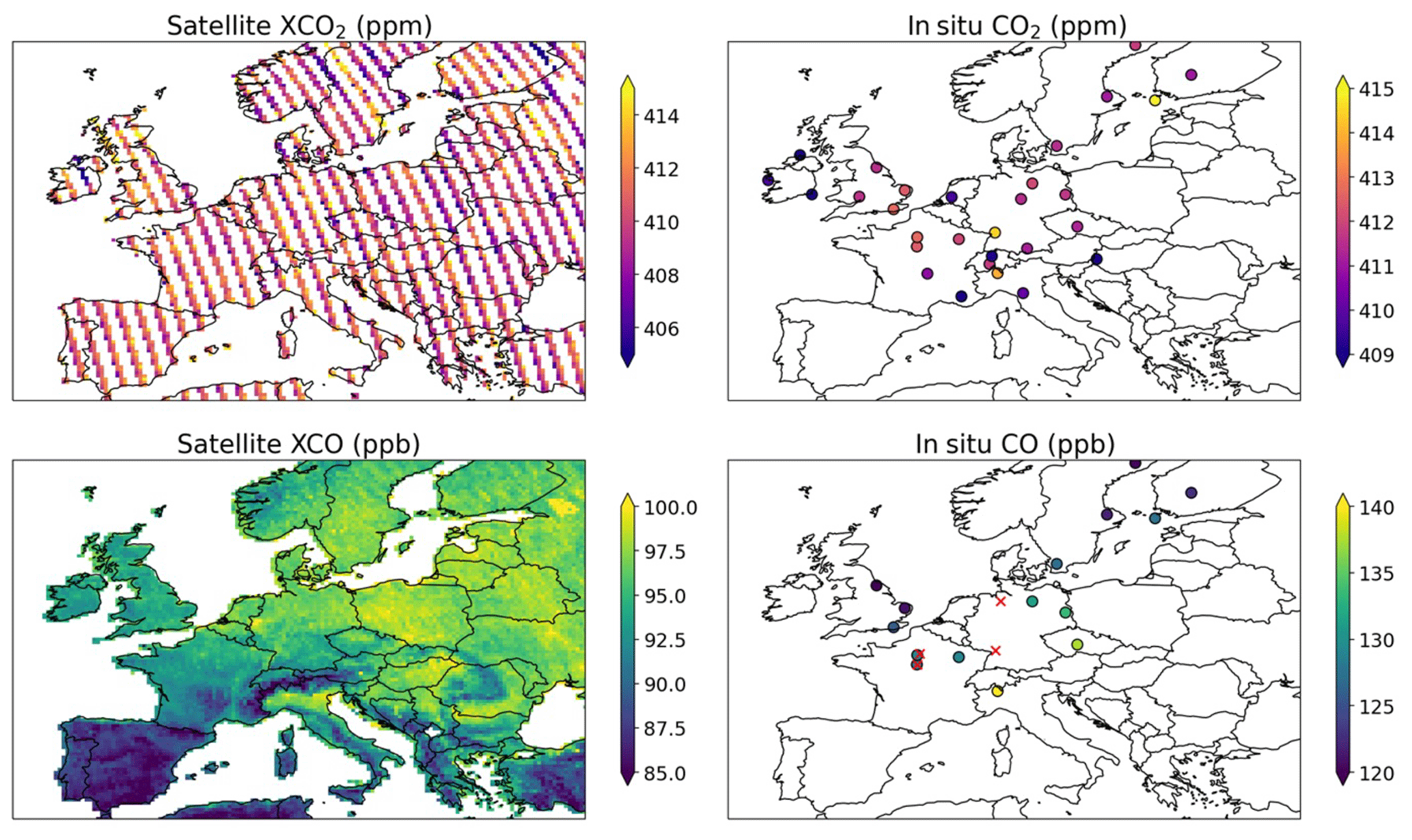
Figure 1 Annual mean CO₂ and CO observed by satellite and in situ networks across Europe for 2018–2021. Satellite observations of XCO₂ and XCO are from OCO-2 and TROPOMI, respectively, and in situ observations are from the DECC and ICOS networks. The red X marks in the in situ CO plot show the locations of four out of the five TCCON sites for which we use XCO₂ and XCO data to evaluate our inversions; the fifth site, based in Cyprus, is located outside the figure domain. The observations are filtered as stated in the text, and satellite observations are shown at 0.25°×0.3125° resolution. TROPOMI observations only include observations after July 2018.

We use in situ observations for 2018–2021 (Fig. 1). We use the DECC surface measurement network in the UK (Stanley et al., 2018; O'Doherty et al., 2024; O'Doherty et al., 2024) and the ICOS measurement network for Europe (ICOS RI et al., 2022). We retain in situ observations collected between 09:00 and 18:00 LT – to avoid instances when tall tower inlets sit above a shallow boundary layer – and then time-average to 3-hourly intervals to match our GEOS FP model meteorology. All in situ sites have CO₂ observations, but some sites are missing CO observations. We additionally remove observations when the atmosphere is not well mixed. We consider the atmosphere to be well mixed when the standard deviation of CO₂ concentrations across the lowest five vertical model levels is smaller than 0.3 ppm; this subjective value is based on 3 times the measurement precision of in situ measurements.

Figure 1 also shows European sites from the Total Carbon Column Observing Network (TCCON). Five sites are within our domain, including Bremen (Germany; Notholt et al., 2022), Karlsruhe (Germany; Hase et al., 2023), Nicosia (Cyprus; Petri et al., 2022), Orléans (France; Warneke et al., 2022), and Paris (France; Té et al., 2022). We use the TCCON observations as an independent comparison for our inversion results.

2.2 Forward model description

The forward model H describes the relationship between a priori flux estimates of CO₂ and CO and the atmospheric observations. We use the GEOS-Chem atmospheric chemistry transport model to relate surface fluxes of CO₂ and CO to 4-D atmospheric concentrations. We then sample these concentration fields at the time and location of measurements. In the case of satellite observations, we also use the scene-dependent averaging kernel to describe the instrument vertical sensitivity to changes in CO₂ and CO. Resulting sampled model atmospheric values can then be compared with observations:

$$\begin{array}{}\text{(1)}& \mathit{y}=\mathbf{H}\cdot \mathit{x},\end{array}$$

where y denotes the observation vector and x denotes the state vector that includes our a priori CO₂ and CO flux estimates.

We use the GEOS-Chem version 12.5.2 atmospheric chemistry and transport model which we run at 0.25°×0.3125° resolution for a nested European domain (−15 to 35° E longitude and 34 to 66° N latitude) with 47 vertical levels. GEOS-Chem is driven by GEOS FP meteorological re-analyses fields from the NASA Global Modelling and Assimilation Office (GMAO) global circulation model.

Our a priori flux estimates (x) include all sources contributing to observed atmospheric CO₂ and CO. Equation (2) shows the sources for CO₂ including combustion emissions (${{\mathrm{CO}}_{\mathrm{2}}}^{\text{Combust}}$), non-combustion fluxes (both biogenic and non-combustion anthropogenic sources; ${{\mathrm{CO}}_{\mathrm{2}}}^{\text{Bio}}$), and background CO₂ that is transported to and from our domain (${{\mathrm{CO}}_{\mathrm{2}}}^{\text{Trans}}$). Atmospheric CO sources include combustion emissions (CO^Combust), transport (CO^Trans), and production of CO through oxidation (CO^Chem), as shown in Eq. (3).

$$\begin{array}{}\text{(2)}& {\displaystyle }{\mathrm{CO}}_{\mathrm{2}}={{\mathrm{CO}}_{\mathrm{2}}}^{\text{Trans}}+{{\mathrm{CO}}_{\mathrm{2}}}^{\text{Combust}}+{{\mathrm{CO}}_{\mathrm{2}}}^{\text{Bio}}\text{(3)}& {\displaystyle }\mathrm{CO}={\mathrm{CO}}^{\text{Trans}}+{\mathrm{CO}}^{\text{Combust}}+{\mathrm{CO}}^{\text{Chem}}\end{array}$$

For our 2018–2021 a priori fluxes, we use a combination of regional and global inventories (Fig. 2). Combustion emissions for both species (${{\mathrm{CO}}_{\mathrm{2}}}^{\text{Combust}}$ and CO^Combust) are from the TNO (Nederlandse Organisatie voor Toegepast Natuurwetenschappelijk Onderzoek; Netherlands Organisation for Applied Scientific Research) GHGco v5.0 emission inventory at 0.1°×0.05° resolution (Super et al., 2020; Kuenen et al., 2022) with national totals based on emissions reported in national inventories and extrapolated from 2019 to more recent years; 2019 represents the latest year for which we have air pollution and greenhouse gas inventories (Kuenen et al., 2022). We apply scaling factors provided by TNO to reflect monthly, hourly, and daily patterns in emissions by sector, with the same scaling factors used for each year. Our combustion source also includes biomass burning emissions from the GFAS v1.2 inventory (Kaiser et al., 2012). Non-combustion fluxes (${{\mathrm{CO}}_{\mathrm{2}}}^{\text{Bio}}$) include ocean fluxes from the NEMO-PISCES model (Lefèvre et al., 2020), lateral carbon fluxes related to crop removal (Deng et al., 2022), and hourly terrestrial biosphere fluxes at $\mathrm{1}/\mathrm{120}\mathit{°}\times \mathrm{1}/\mathrm{60}\mathit{°}$ resolution produced by the VPRM model following methods described by Gerbig (2021) driven by ERA5 meteorology. We include non-combustion (e.g. fugitives) anthropogenic emissions from the TNO inventory in our non-combustion fluxes. Fugitive emissions of CO₂ are typically very small, e.g. emissions that escape from agricultural greenhouses enriched with CO₂.

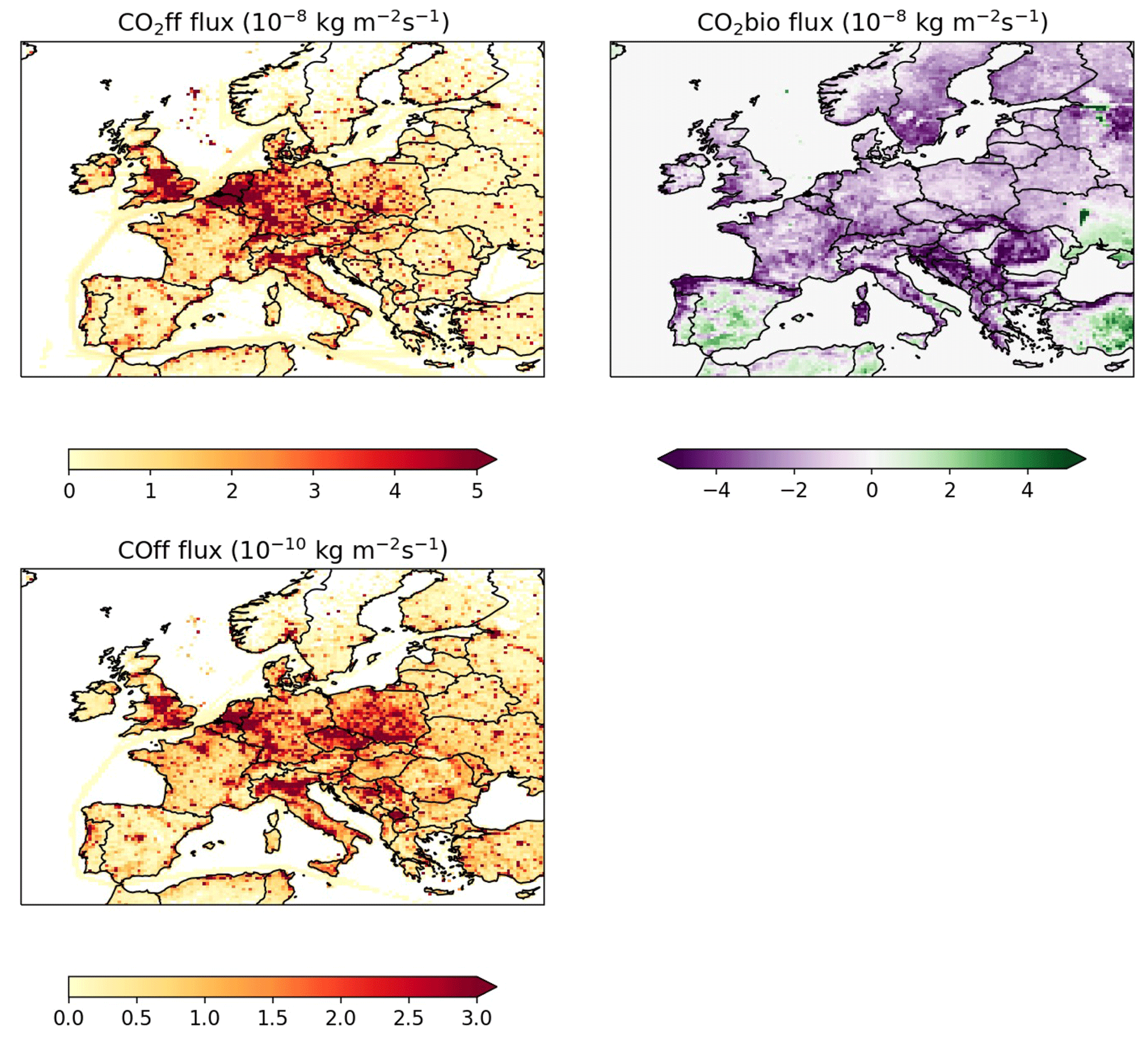
Figure 2 Annual mean emissions for 2018–2021 in the a priori inventories. Combustion emissions (${{\mathrm{CO}}_{\mathrm{2}}}^{\text{combust}}$, CO^combust) are from the TNO inventory, while biogenic fluxes (${{\mathrm{CO}}_{\mathrm{2}}}^{\text{bio}}$) are from the VPRM model (negative values indicate a CO₂ sink).

For our nested domain, we use lateral boundary conditions for CO₂ (${{\mathrm{CO}}_{\mathrm{2}}}^{\text{Trans}}$) from the Copernicus Atmosphere Monitoring Service (CAMS) inversion-optimized global greenhouse gas analysis with assimilation of in situ observations (Chevallier, 2020). Our boundary conditions for CO (CO^Trans) are from the CAMS global reanalysis (Inness et al., 2019). We use the CAMS fields at their provided temporal resolution (3-hourly) and re-grid them to the GEOS-Chem horizontal spatial resolution of 2°×2.5° so we can use them as boundary conditions for our finer-resolution nested model, centred over Europe. Because the vertical resolution of GEOS-Chem does not align with CAMS, we translate the CAMS native vertical resolution to our 47 model layers using linear interpolation of logarithmic pressure values. We fill in the species concentrations at the lowest or highest pressure level in CAMS for the top or surface of the atmosphere, respectively, when the GEOS-Chem pressure levels go beyond the bounds of CAMS.

We treat the relationship between surface fluxes and concentrations (Eq. 1) as linear (e.g. a doubling of emissions leads to a doubling of the atmospheric signal). To linearize the CO simulation, we use offline chemistry terms to represent the chemical production of CO (CO^Chem). CO is primarily produced by oxidation of methane and non-methane volatile organic compounds by the hydroxyl radical (OH), so we generate the production terms using offline 3-D loss fields of OH generated from a previous GEOS-Chem full-chemistry simulation (Fisher et al., 2017).

2.3 Inverse model description

For our inversion, we use the ensemble Kalman filter (EnKF) approach as discussed in detail by others (e.g. Peters et al., 2005; Hunt et al., 2007; Feng et al., 2009; Liu et al., 2016). We specifically follow the methods derived by Hunt et al. (2007) and summarized by Liu et al. (2016) for the local ensemble transform Kalman filter (LETKF).

We solve the inversion in ensemble space rather than for the state vector elements. For each state vector element, we have an ensemble of potential scale factors that follow our prescribed error statistics. For each assimilation time period (over which we ingest observations), we solve for the mean a posteriori state vector (${\stackrel{\mathrm{‾}}{\mathit{x}}}^a$) that represents the mean of our N ensemble members (where we use N=100):

$$\begin{array}{}\text{(4)}& {\stackrel{\mathrm{‾}}{\mathit{x}}}^a={\stackrel{\mathrm{‾}}{\mathit{x}}}^b+\mathbf{K}({\mathit{y}}_{\text{obs}}-{\stackrel{\mathrm{‾}}{\mathit{y}}}^b),\end{array}$$

where ${\stackrel{\mathrm{‾}}{\mathit{x}}}^a$ and ${\stackrel{\mathrm{‾}}{\mathit{x}}}^b$ are the means across ensemble members for our a posteriori and a priori state vectors, respectively. We use error statistics, as described in Sect. 2.4, to generate the a priori state vector ensemble members. y_obs is the observation vector, and each element of ${\stackrel{\mathrm{‾}}{\mathit{y}}}^b$ is the mean of model-predicted concentrations across N ensemble members. For the nth ensemble member (${\mathit{x}}_n^b$), the model-predicted concentrations are ${\mathit{y}}_n^b=H\left({\mathit{x}}_n^b\right)$.

K describes our Kalman gain matrix that regulates the degree to which any disagreement between model and observation will adjust the state vector. We determine K using the matrix x^b, which describes the difference between the ensemble members and their mean, and the matrix y^b, which describes the difference between the model-predicted concentrations and their mean:

$$\begin{array}{}\text{(5)}& \mathbf{K}={\mathit{x}}^b{\stackrel{\mathrm{̃}}{\mathbf{P}}}^a({\mathit{y}}^b{)}^{\mathrm{T}}{\mathbf{R}}^{-\mathrm{1}},\end{array}$$

where the nth column of x^b is ${\mathit{x}}_n^b-{\stackrel{\mathrm{‾}}{\mathit{x}}}^b$ and the nth column of y^b is ${\mathit{y}}_n^b-{\stackrel{\mathrm{‾}}{\mathit{y}}}^b$ (each column representing an ensemble member). R is the observation error covariance matrix, which includes the errors from our forward model, from estimates based on prior studies, and from observations. For CO₂, we use an a priori model error of 1.5 ppm for the satellite inversion (Feng et al., 2017) and 3 ppm for the in situ inversion (within the range of Monteil et al., 2020, and White et al., 2019). For CO, we use an a priori model error of 15 and 20 ppb for the satellite and in situ inversions, respectively (Northern Hemisphere CO column and surface mole fraction model–observation differences from Bukosa et al., 2023). For the observations, we use the errors as provided for the satellite or in situ network, averaged to the model resolution. We generate the off-diagonal covariance for R based on the spatial and temporal proximity of observations following an exponential decay with spatial and temporal length scales of 100 km and 4 h, respectively; these values are based on our preparatory work (not shown) using this model definition.

The ${\stackrel{\mathrm{̃}}{\mathbf{P}}}^{\mathrm{a}}$ matrix is a representation of the a posteriori error covariance in ensemble space:

$$\begin{array}{}\text{(6)}& {\stackrel{\mathrm{̃}}{\mathbf{P}}}^a=\left[\right(N-\mathrm{1})\mathbf{I}+({\mathit{y}}^b{)}^{\mathrm{T}}{\mathbf{R}}^{-\mathrm{1}}{\mathit{y}}^b{]}^{-\mathrm{1}},\end{array}$$

where I is an identity matrix and N is our number of ensemble members. ${\stackrel{\mathrm{̃}}{\mathbf{P}}}^a$ is used to determine the a posteriori ensemble members (x^a), where the nth column of x^a is ${\mathit{x}}_n^a-{\stackrel{\mathrm{‾}}{\mathit{x}}}^a$, and the error covariance matrix (P^a):

$$\begin{array}{}\text{(7)}& {\displaystyle }{\mathit{x}}^a={\mathit{x}}^b\left[\right(N-\mathrm{1}){\stackrel{\mathrm{̃}}{\mathbf{P}}}^a{]}^{\mathrm{1}/\mathrm{2}},\text{(8)}& {\displaystyle }{\mathbf{P}}^a={\mathit{x}}^a\left({\mathit{x}}^a{)}^T\right(N-\mathrm{1}{)}^{-\mathrm{1}}.\end{array}$$

We use an assimilation window of 2 weeks and a lag window of 1 month, accounting for the impact of historical emissions on our assimilation period. This means that the state vector for each time step includes scale factors for the assimilation window and lag window. Our preparatory work revealed that using a lag window longer than a month did not significantly impact our results because signals by that time have decayed substantially (not shown). We perform our inversion sequentially, using the a posteriori scale factors for a given assimilation window to update the a priori scale factors for the next lag window over the same date range. To avoid unrealistically small prior uncertainties, we apply a 10 % error inflation when we update the a priori state vector.

The benefit of the LETKF is that we can localize the inversion so that each state vector element is only influenced by a subset of observations. For our inversions using in situ observations, we localize by distance so that each state vector element that represents a grid-scale variable is only influenced by observations within a 1000 km range. We chose that upper limit as a compromise to ensure we included observations that had the most sensitivity to the emissions and to discard observations with much smaller sensitivities that potentially could introduce spurious correlations.

2.4 Description of inverse model experiments

We test different approaches to investigate the usefulness of satellite observations for evaluating CO₂ combustion emissions. The approaches vary in the observations that are used and the representation of error covariances for our a priori estimates. For each type of inversion, we compare our satellite inversion results to comparable inversions using in situ observations.

In the inversions, instead of solving for CO₂ or CO fluxes, we solve for scale factors that scale up or scale down the source terms from Eqs. (2) and (3). We first assume that our a priori scale factors are all equal to 1. We solve for a posteriori scale factors that, when applied to our source terms, will result in modelled atmospheric CO₂ or CO concentrations in better agreement with observations.

For our first approach (CO₂-only), we perform a CO₂-only inversion that assimilates CO₂ observations. Our state vector includes scale factors for the sources of Eq. (2):

$$\begin{array}{}\text{(9)}& {\mathit{x}}_{\text{co2}}=({\mathit{x}}_{\text{co2}}^{\text{Trans}},{\mathit{x}}_{\text{co2}}^{\text{Bio}},{\mathit{x}}_{\text{co2}}^{\text{Combust}}),\end{array}$$

where ${\mathit{x}}_{\text{co2}}^{\text{Bio}}$ and ${\mathit{x}}_{\text{co2}}^{\text{Combust}}$ are a vector of scalers, common to all inversions, with each element applying to a non-combustion or combustion grid cell at 0.5°×0.625° resolution (Appendix A). The four transport scale factors for CO₂ (and four for CO), described by ${\mathit{x}}_{\text{co2}}^{\text{Trans}}$, common to all our inversion calculations, apply to the four lateral boundary conditions of the nested model domain.

In our second approach (joint CO₂:CO), we perform a joint CO₂:CO inversion that assimilates both CO₂ and CO observations. For the joint inversion, we assume there is 100 % correlation for the CO₂ and CO combustion emission errors. This means any adjustment made by our inversion to the CO₂ combustion scale factors will also apply to the CO scale factors and vice versa. We can then use a common combustion scaling term for both species in our state vector (x^Combust). We do not account for the atmospheric CO₂ production from the oxidation of CO and other reduced carbon species (Suntharalingam et al., 2005). Our state vector also includes four scale factors for lateral boundary transport of each species (as described above). For CO we also include two scale factors to the state vector for the chemistry terms (${\mathit{x}}_{\text{co}}^{\text{Chem}}$), describing the secondary production of CO from the oxidation of methane and non-methane volatile organic compounds. The two scale factors reflect differences in their emission distributions and atmospheric lifetimes. The CO₂ and CO state vectors are described as

$$\begin{array}{}\text{(10)}& {\mathit{x}}_{\text{co2}}=\left({\mathit{x}}_{\text{co2}}^{\text{Trans}},{\mathit{x}}_{\text{co2}}^{\text{Bio}},{\mathit{x}}^{\text{Combust}}\right),\end{array}$$

$$\begin{array}{}\text{(11)}& {\mathit{x}}_{\text{co}}=\left({\mathit{x}}_{\text{co}}^{\text{Trans}},{\mathit{x}}_{\text{co}}^{\text{Chem}},{\mathit{x}}^{\text{Combust}}\right).\end{array}$$

For our first two approaches, we assume an a priori uncertainty of 20 % (relative standard deviation) for the combustion scale factors (x^Combust). We use an a priori uncertainty of 50 % for the non-combustion scale factors (${\mathit{x}}_{\text{co2}}^{\text{Bio}}$) and 5 % for the atmospheric transport and chemistry scale factors. These are informed estimates based on our previous work, e.g. Feng et al. (2017). For our non-combustion and combustion scale factors, we generate error covariances for nearby grid cells that exponentially decay with increasing distance. Our method for generating the error covariance matrix based on these uncertainties is described in detail in Appendix A.

We acknowledge that the assumption of 100 % error correlation for CO₂ and CO combustion emissions is likely to be a gross overestimate, but it serves as an illustrative upper limit for our calculations. For example, we may underestimate CO emissions due to an underestimate of incomplete combustion activities, and this will not translate to the same underestimate in CO₂.

For our third approach (TNO CO₂:CO), we test this assumption by solving for the CO₂ and CO combustion scaling terms separately:

$$\begin{array}{}\text{(12)}& {\displaystyle }{\mathit{x}}_{\text{co2}}=\left({\mathit{x}}_{\text{co2}}^{\text{Trans}},{\mathit{x}}_{\text{co2}}^{\text{Bio}},{\mathit{x}}_{\text{co2}}^{\text{Combust}}\right),\text{(13)}& {\displaystyle }{\mathit{x}}_{\text{co}}=\left({\mathit{x}}_{\text{co}}^{\text{Trans}},{\mathit{x}}_{\text{co}}^{\text{Chem}},{\mathit{x}}_{\text{co}}^{\text{Combust}}\right).\end{array}$$

We call this our TNO approach because we use estimates of the uncertainties in the TNO emission inventory to create our error covariance matrix (Super et al., 2024). We increase the provided uncertainties by a factor of 3 to make them more comparable with our other simulations. This results in a mean grid-scale CO₂ combustion uncertainty of 18 %, though there is greater variability in grid cell uncertainties compared to our other approaches. We expect higher correlation between CO₂ and CO gridded emissions in regions where the same spatial product (e.g. road network maps) is used to distribute emissions for both species and that spatial product has high uncertainties. The spatial products and how they are used to distribute air pollutant emissions are described by Kuenen et al. (2022).

3 Results and discussion

First, we describe the comparison between our a priori and a posteriori model simulations against observations. We then report our a posteriori CO₂ fluxes for Europe and its constituent countries and the UK.

3.1 Inversion performance

Our a priori CO₂ emissions are already consistent with data from the five relevant TCCON sites (locations shown in Fig. 1; Pearson correlation coefficient R=0.87) and in situ (R=0.76) and satellite (R=0.84) observations. The model has a small, positive relative mean bias compared to TCCON (0.7 %) and a very small bias compared to in situ and satellite observations (0.2 %). Table A1 reports a statistical summary of the model–observation comparisons. The satellite inversions show improvement for the model–satellite fit (R=0.92–0.95), as expected, and the model–in situ fit (R=0.80–0.82). Similarly, the in situ inversions improve model–in situ fit (R=0.83–0.84) and to a lesser extent the model–satellite fit (R=0.85–0.87).

In general, including CO and TNO uncertainty estimates improves the model–observation fit and reduces the mean bias. For example, the satellite joint CO₂:CO (R=0.93) and TNO (R=0.92) inversions show the greatest improvement in fit with TCCON. The one exception is that the mean bias compared to TCCON is slightly larger with CO (0.3 %–0.5 %) compared to CO₂-only (0.2 %–0.4 %), a small difference that is likely a result of introducing the CO:CO₂ error correlation. The TCCON CO₂ bias is seasonal (not shown), with the a priori model showing no bias in July–August and a positive bias of 1–4 ppm for the rest of the year. The in situ inversions reduce the mean bias for March–June by 1 ppm, and this improvement lines up with a reduction in the biosphere sink for these inversions (discussed later). We also compare our a priori and a posteriori fields with TROPOMI CO, but the improvement is marginal. The Pearson correlation coefficient between the a posteriori model and in situ data increases by 4 % for the joint CO₂:CO inversion and by 5 % for the TNO joint inversion. For a similar comparison but using satellite data, the correlation coefficient increases by 6 % for the joint CO₂:CO inversion and by 4 % for the TNO joint inversion.

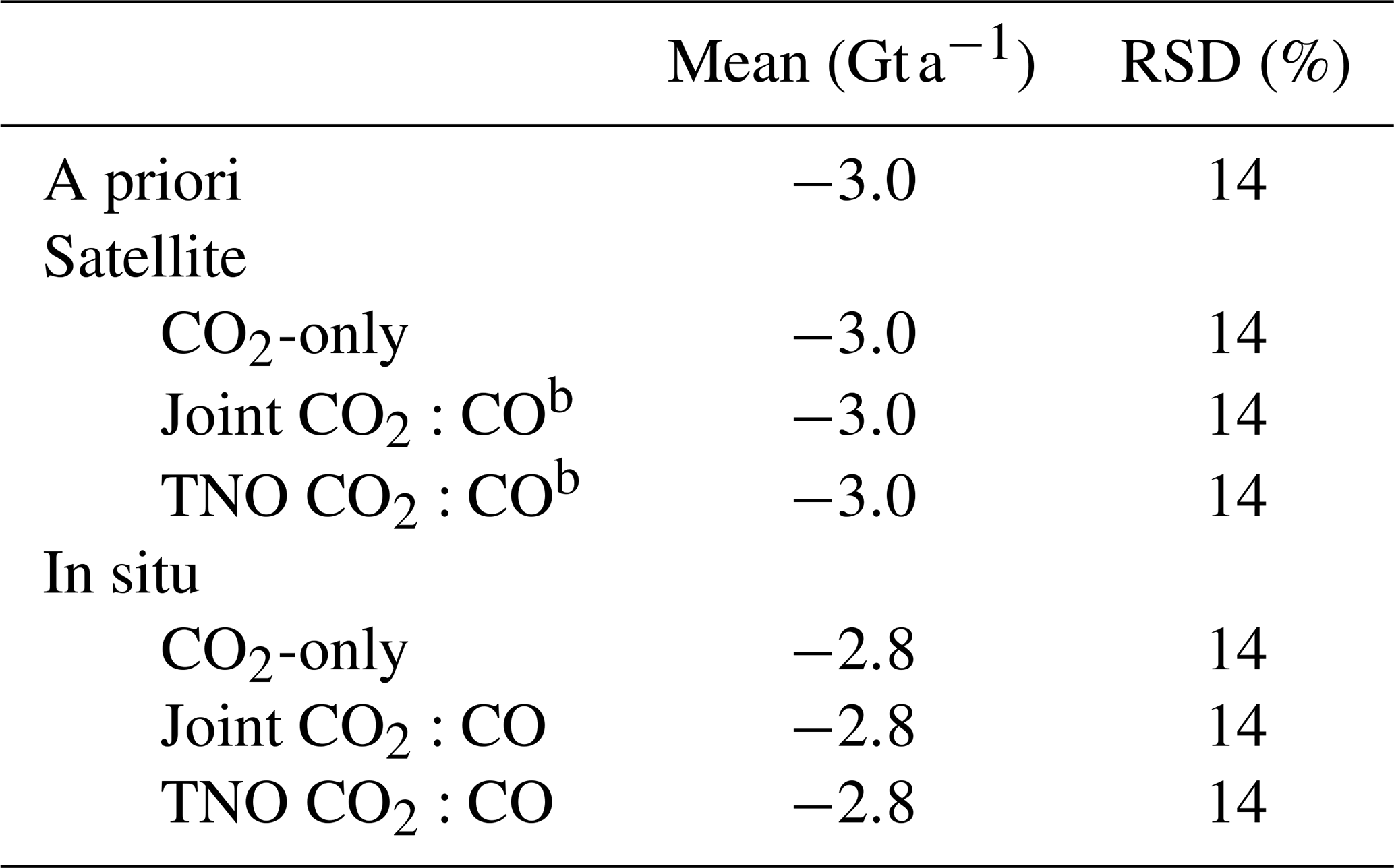
We also assess inversion performance by the degree of uncertainty reduction for the a posteriori CO₂ combustion emission estimates. Table 1 shows a posteriori uncertainties for our domain-scale CO₂ combustion emissions. The reductions in relative uncertainty achieved at the domain scale for all inversions are small (6 %–12 %), with the CO₂-only and TNO satellite inversions showing no reduction. The TNO inversions show smaller reductions in uncertainty (0 %–6 %) compared to the joint inversions (8 %–12 %), but they also start with a lower a priori uncertainty at 1.6 % (relative standard deviation, RSD = sample standard deviation $/$ sample mean) compared to 2.4 % for non-TNO a priori uncertainties.

Table 1 Average domain CO₂ combustion emissions for 2018–2021.

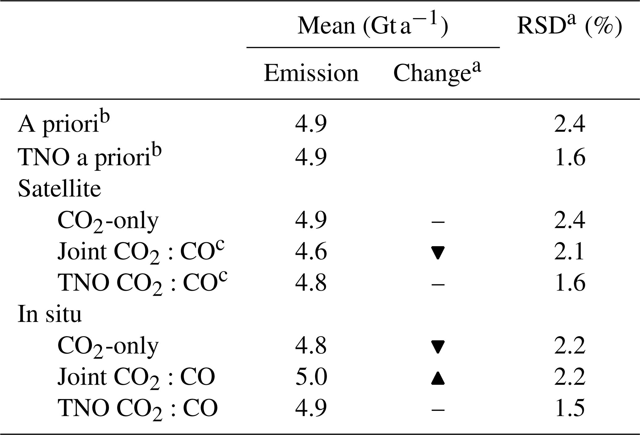
^a The arrows indicate the change in the mean from the a priori emission estimate. Downward-pointing arrows show a decrease, the upward-pointing arrow shows an increase, and dashes show no change. RSD stands for relative standard deviation. ^b The a priori uncertainty labelled as “A priori” is for the CO₂-only and joint inversions, so we also include the a priori uncertainty for the TNO inversion. ^c The joint and TNO satellite inversions only include July 2018–December 2021. The a priori combustion emission for this period is 4.8 Gt a⁻¹, so we show no change for the TNO a posteriori emissions.

At the national scale, we see the greatest uncertainty reduction in CO₂ combustion emissions for the top 10 emitting countries when satellite CO observations or in situ CO₂ measurements are included and the non-TNO uncertainties are used (Tables A2 and A3). The average uncertainty reductions for the joint satellite and CO₂-only in situ inversions are 11 % and 9 %, respectively. This is not surprising given the greater number of observations provided by these two platforms and increased sensitivity to surface fluxes compared to OCO-2. Including in situ CO observations in the inversion does not improve the national-scale uncertainty reduction. Because we use lower a priori uncertainties in the TNO inversion (national scale 2 %–10 % RSD) compared to the other inversions (6 %–14 % RSD), fewer countries have reduced uncertainties for the TNO inversion, though a posteriori uncertainties are reduced in the Netherlands (2 %) for in situ and satellite observations compared to a priori uncertainties (3 %).

3.2 Emission estimates for the UK and mainland Europe

Table 1 shows our mean domain-scale (includes the UK and mainland Europe) combustion emissions for 2018–2021. The inversions show a small decrease or no change from the a priori emissions (4.9 Gt a⁻¹), except for the joint satellite and in situ inversions that show a larger decrease (4.6 Gt a⁻¹) and an increase (5.0 Gt a⁻¹) from the a priori emission estimates, respectively. Figure 3 shows that the joint satellite inversion decreases combustion emissions year-round for all years, with the greatest decreases in winter. The TNO satellite and in situ and CO₂-only in situ inversions also show decreases in the winter and early spring (Figs. 3 and 4), providing more confidence in this scaling down of emissions.

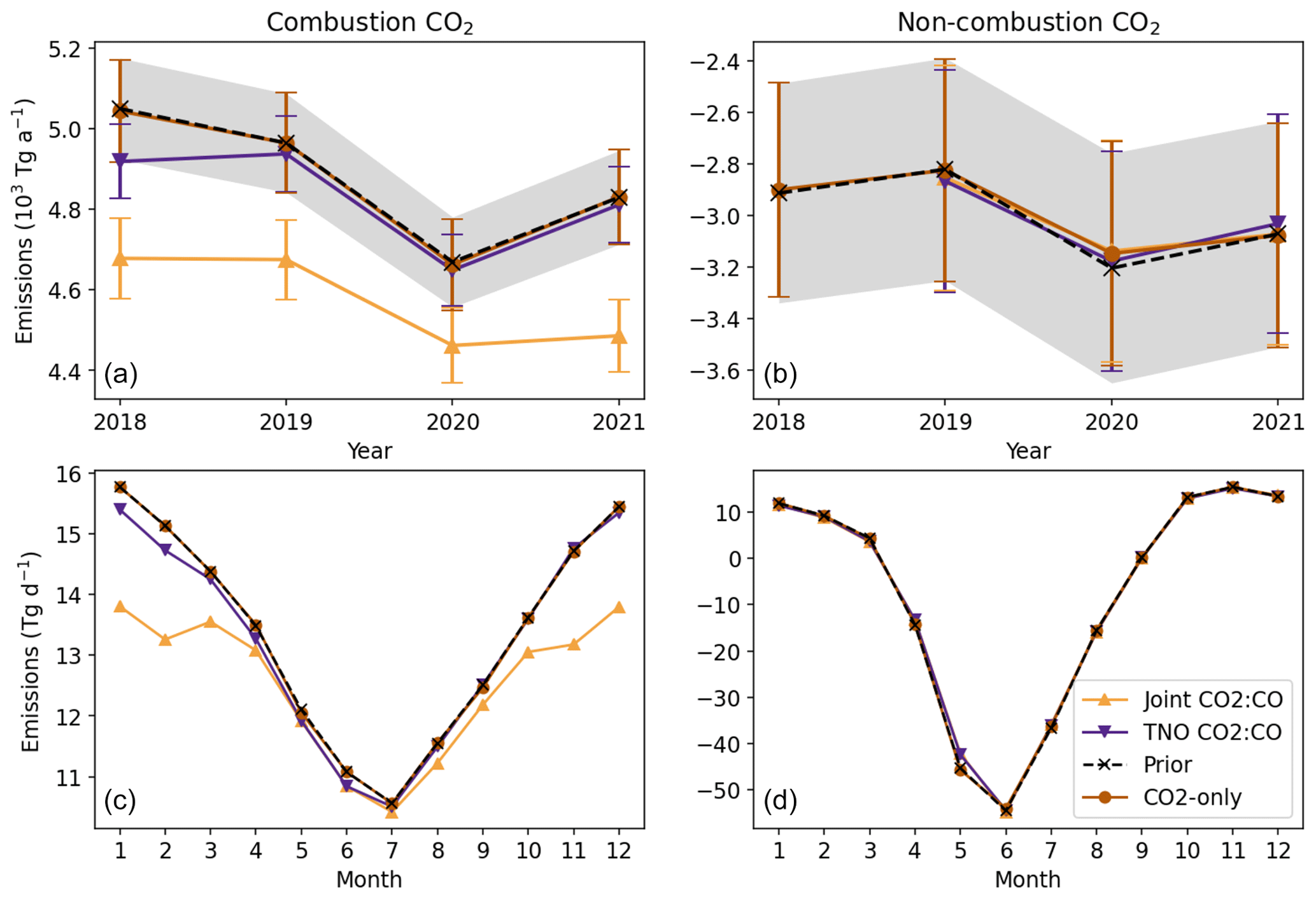
Figure 3 Annual and monthly mean European CO₂ combustion and non-combustion emissions inferred from satellite inversions for 2018–2021. The non-combustion emissions include biogenic and non-combustion anthropogenic emission sources. The top row (a, b) shows annual mean CO₂ flux estimates by inversion type, with errors bars showing the 1σ errors except for the a priori errors which are shown as a shaded region. The bottom row (c, d) shows monthly mean fluxes for 2018–2021. The TNO and joint inversions only include July 2018–December 2021 for combustion and 2019–2021 for non-combustion. Please note the differences in the range used for the y axes.

Figure 4 The same as Fig. 4 but for in situ inversions.

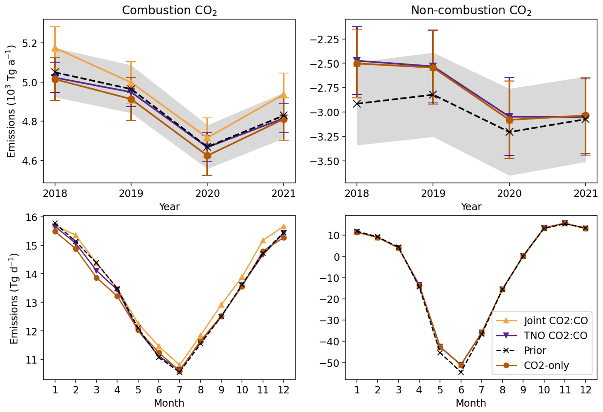
In contrast, the joint in situ inversion is higher than the a priori values for all months and all years (Fig. 4). This pattern is not reflected in our other inversion approaches and is likely, in part, due to the model underestimating the fine-scale variability in CO compared to what is measured at some in situ sites combined with the use of a common scale factor for both CO and CO₂, leading to an over-correction upward of combustion emissions. For example, we find that removing a single site close to an urban region in northern Italy (Ispra ICOS site) reverses the sign of scaling in the region from an increase to a decrease. The disagreement between satellite and in situ CO₂:CO inversions is less pronounced for the TNO inversions because the separation of CO₂ and CO in our state vector prevents the CO underestimates from heavily influencing the CO₂ combustion emissions.

Figure 3 shows a slight (1 %) decrease in mean a priori combustion emissions from 2018 to 2021, and all satellite and in situ inversion results show a similar trend (Figs. 3 and 4). The mean a priori non-combustion (biogenic) CO₂ sink shows a slight increase (1 %) for 2018–2021, and the inversion results show a similar (satellite; Fig. 3) or greater increase (in situ; Fig. 4) in the CO₂ sink. Figure 4 shows the monthly mean biogenic CO₂ sink is weakened for the in situ inversions, mostly in summer, whereas Fig. 3 shows almost no change in the sink for the satellite inversions (also listed in Table A4), indicating that the CO₂ in situ observations, due to the coverage and sensitivity they provide, are needed for constraining biogenic flux estimates.

The differences between a posteriori and a priori annual emissions for all inversions except the joint satellite inversion are not statistically significant and remain within the 1σ uncertainties of the a priori estimate. The inter-annual trends are also smaller in magnitude than the a posteriori uncertainties, making it difficult to assess if CO₂ combustions in Europe have decreased from 2018 to 2021. For the joint satellite and in situ inversions, we assumed that CO was a strong tracer for CO₂ combustion emissions on this regional scale by using a common scale factor, but we find that this assumption leads to more extreme, likely unrealistic, divergence from the a priori emission estimates, in disagreement with the other inversion results. This reflects the difficulties of using CO as a tracer for CO₂ combustion emissions at regional scales and the importance of error characterization.

3.3 National-scale emission estimates

Figure 5 shows national CO₂ combustion emissions for the top 10 emitting countries in our European domain (also listed in Tables A2 and A3). Germany is the highest emitter, with an a priori emission of 821 Tg a⁻¹. Most inversions show a decrease in Germany's emissions (717–806 Tg a⁻¹), except for the in situ joint inversion, which shows an increase (830 Tg a⁻¹), and the CO₂-only inversion, which shows little change from the a priori estimate (819 Tg a⁻¹). The other top emitting countries, including Poland, the UK, France, Italy, Spain, Belgium, the Czech Republic, the Netherlands, and Romania, show emission decreases for the satellite joint (3 %–17 %) and TNO (0 %–4 %) inversions. The in situ CO₂-only and TNO inversions generally show only small changes (<1 %) in national emissions except for a 4 % national emission decrease in the Netherlands and Belgium for the CO₂-only inversion.

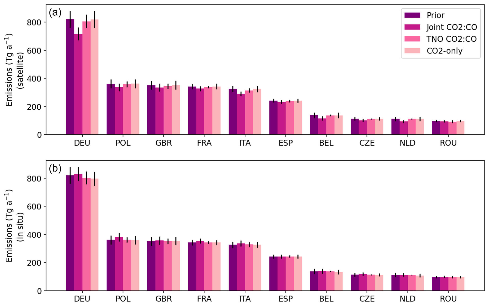
Figure 5 Annual mean a priori and a posteriori CO₂ combustion emissions by country for satellite (a) and in situ (b) inversions. We show the top 10 emitting countries in our European domain with emissions averaged over 2018–2021. The TNO and joint satellite inversion averages do not include dates prior to July 2018.

The joint inversions show the largest changes in national emissions but in opposite directions. In contrast, the TNO inversions show smaller changes from the a priori emission estimates (in part, due to the lower a priori uncertainties) and better agreement, including agreement in Germany where there is greater divergence from the a priori estimate (2 % decrease for both TNO inversions).

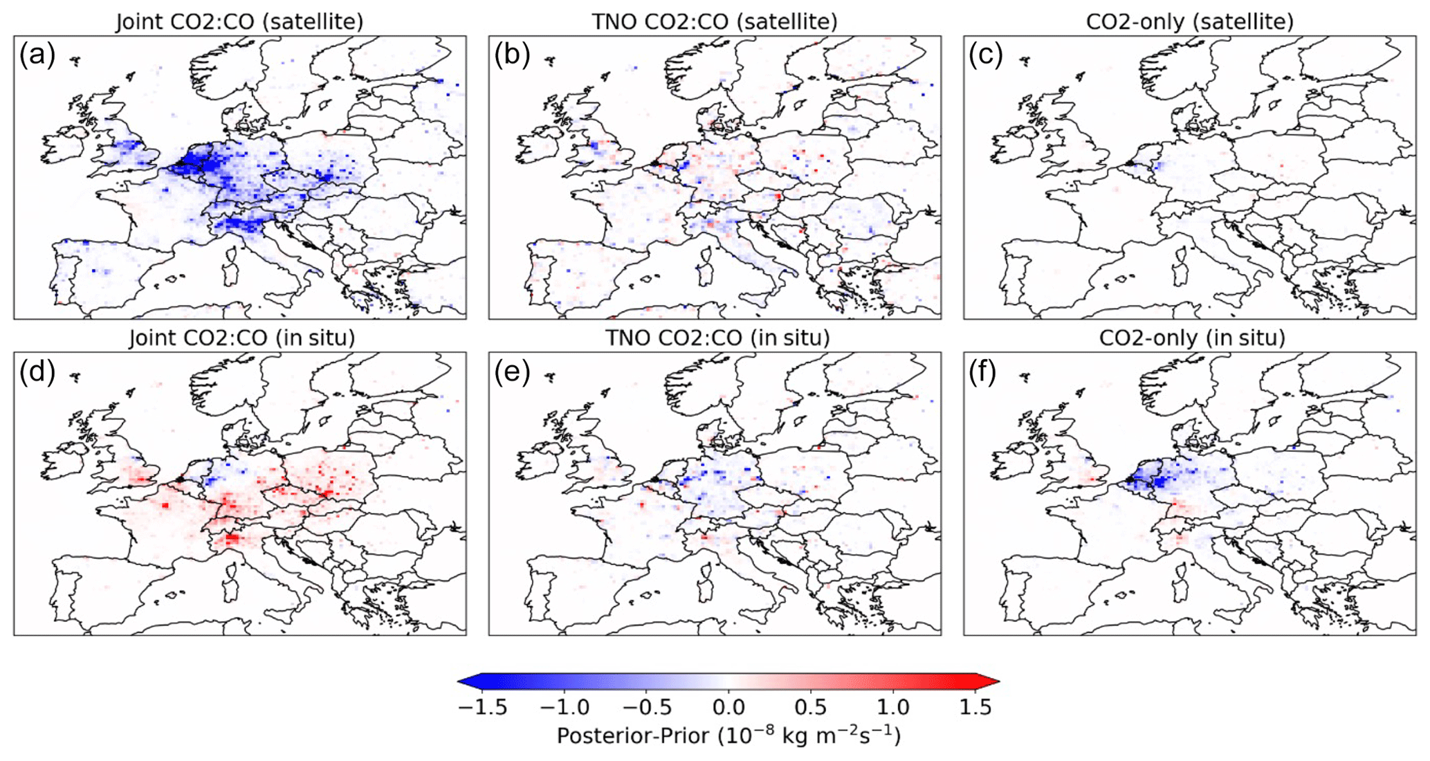
Figure 6 Annual mean CO₂ combustion emissions difference (a posteriori minus a priori) for satellite (a–c) and in situ (d–f) inversions, 2018–2021, shown at the native model resolution of 0.25°×0.3125°. The TNO and joint satellite inversion averages do not include dates prior to July 2018.

Despite the national-scale disagreements for some inversions, we find regional corrections to combustion emissions are consistent for all inversions. Figure 6 shows that the populated North Rhine-Westphalia region in western Germany shows a posteriori CO₂ combustion emission estimates are smaller than a priori values for all inversions. The TNO and CO₂-only inversions show mixed corrections in Poland, with TNO inversions showing the best agreement. Most inversions, including both TNO inversions, show an increase in emissions near Milan and Vienna, but over other major cities like Paris, Madrid, and London there is less agreement in the sign and magnitude of the emissions changes.

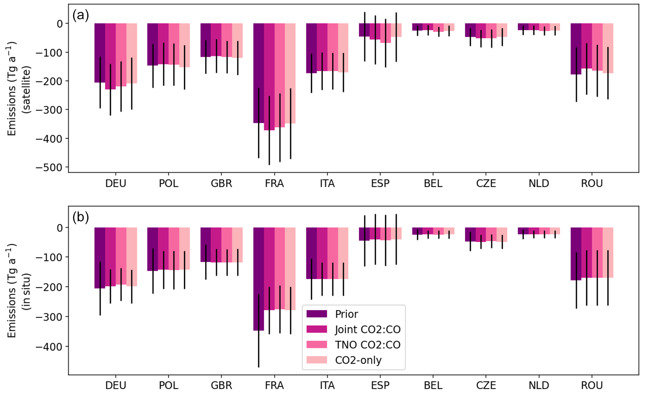
Figure 7 As Fig. 5 but for non-combustion CO₂ flux estimates. The TNO and joint satellite inversion averages do not include 2018. The non-combustion emissions include biogenic and non-combustion anthropogenic emission sources.

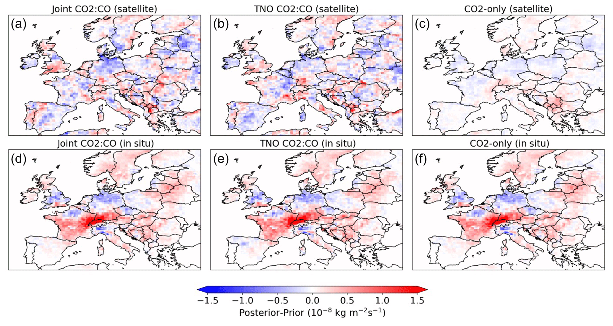
Figure 8 As Fig. 6 but for non-combustion CO₂ flux estimates. The TNO and joint satellite inversion averages do not include 2018. The non-combustion emissions include biogenic and non-combustion anthropogenic emission sources.

The differences in the joint inversions are due to contrasting corrections to CO emissions that carry over into the CO₂ emissions. Figures A1 and A2 show that the in situ joint inversion shows decreases for high-emitting regions in Europe for winter and spring, but this is mostly offset by large emission increases in summer and fall. In contrast, the satellite joint inversion shows decreases for all seasons. For the TNO inversion, there is less disagreement between the seasonal emissions corrections for CO₂, but there are disagreements in CO corrections. Figure A3 shows the CO corrections for the TNO inversion generally occur at the national scale, and we know there is low error correlation between the two species at the national scale (Super et al., 2024), so it is not surprising that these corrections do not carry over to CO₂. The improvement in the agreement between our a posteriori CO emissions and TROPOMI and in situ CO measurements, relative to our a priori emissions, is larger than for the similar comparison using CO₂. This reflects the larger assumed CO errors. A posteriori CO estimates agreed better with these measurements for the joint CO₂:CO and the TNO inversions, with the TNO inversion performing slightly better.

Figure 7 shows national non-combustion (biogenic) emissions for the countries in Fig. 5. All countries show a net sink, with France having the largest net sink. The in situ inversions tend to decrease (lessen) the CO₂ sink for all countries and reduce uncertainties. Figure 8 shows the spatial pattern in the flux changes is consistent for all in situ inversions. In contrast, the national CO₂ biogenic fluxes show little change from the a priori emission estimates for the satellite inversions, highlighting the importance of in situ CO₂ observations for constraining biogenic flux estimates. For all inversions, the CO₂ sink in northern Germany is strengthened (more negative fluxes) and it is weakened in southern Germany and Switzerland, though there are conflicting corrections in surrounding regions such as France and northern Italy. These disagreements may be due to the differing observing capacities with satellites having seasonal limitations due to snow and clouds. We find low a posteriori error correlations between national-scale combustion and biogenic fluxes (mostly R<0.1, except for Germany $R=-\mathrm{0.2}$), indicating that the disagreement in in situ and satellite a posteriori biogenic fluxes will not carry over into combustion emission estimates.

4 Conclusions

We find that using CO₂ satellite observations from OCO-2 alone cannot reproduce a posteriori European CO₂ fluxes inferred from the European in situ CO₂ measurement network. The satellite observations (CO₂-only) do not show significant combustion emissions changes from our a priori estimates, whereas when we use in situ CO₂ or CO₂ and CO satellite observations, we see greater divergence from the a priori emissions. This is likely due to in situ data being more sensitive to emissions and to coverage provided by the current generation of satellites being insufficient to significantly update the state vector. We find that the in situ network is still essential for constraining biogenic fluxes, though we also find low correlation between combustion and biogenic fluxes, indicating that our inability to constrain the biogenic flux estimate using satellites does not prevent the estimation of combustion emissions at the national scale using satellite observations.

All our inversions indicate that CO₂ combustion emissions for regions of Germany are overestimated in winter, and most inversions show this overestimate extends to other countries in Europe. We also find that the in situ inversions show a smaller summertime European CO₂ sink, which is not shown for the satellite inversions. We find that the existing observational networks are not able to significantly reduce the errors for our European or national emission estimates to the extent necessary for distinguishing inter-annual emission trends that represent only a few percent of total emissions.

When using CO as a tracer for CO₂ combustion emissions in our inversion system, we find that our interpretation of inversion results is highly dependent on the assumptions of a priori error correlation between CO and CO₂. The use of a CO:CO₂ inversion system can potentially improve our ability to track CO₂ combustion emissions provided we have well-characterized error correlations between the two species which may require broad measurement-based studies to determine the error correlations specific to a source and region. This suggests that the increase in observational capacity for CO₂ and co-emitted trace gases promised by the Copernicus CO₂ Monitoring (CO2M) satellite mission has the potential to improve our ability to constrain national combustion emission estimates provided that the error correlations for CO₂ combustion emissions and the co-emitted species are strong and well characterized using empirical data.

In general, the improvements in model–observation fit are small, and we do not see a significant reduction in uncertainties compared to our a priori estimates. This is expected because we have extensive knowledge about sector emissions that underpin these regional inventories, reflected in the small uncertainties associated with combustion emission estimates across the UK and mainland Europe. The use of CO observations and TNO error estimates leads to better agreement between satellite and in situ inversions and the best model–observation fit, though including CO does not reduce the model bias compared to TCCON and likely reflects the need for in situ CO₂ observations for reducing biases related to biogenic fluxes. Despite the sensitivity of our a posteriori emission estimates to the choice of a priori CO₂ and CO uncertainties, the joint and TNO satellite inversions perform similarly when compared to TCCON. This highlights the need for not only further satellite observing capacity but also improved ground-based networks for evaluating satellites and the usefulness of including co-emitted species observations.

Appendix A: Description of an a priori ensemble generation

For the a priori ensemble perturbations that represent our state vector (${\mathit{x}}_n^b$ for the nth ensemble member), we generate an ensemble of scale factors based on the desired error statistics, described in Sect. 2.3. For the combustion and non-combustion scale factors, we solve for scale factors on a 0.5°×0.625° resolution grid (double our nested model resolution). Each ensemble member is then a grid of perturbations that we will apply to our emissions grid. To generate the ensemble members, we first generate an error covariance matrix (P):

$$\mathbf{P}={\mathbf{P}}^{\prime }\cdot \left(e^{-\frac{\mathbf{D}}{\mathrm{100}}}\cdot {\mathbf{P}}^{\prime }\right),$$

where P^′ is a diagonal matrix with the variance for each state vector element along its diagonal. Covariance between grid cells is based on the spatial proximity between each grid cell and its neighbor, with distances between grid cells represented by the matrix D. The influence of neighboring grid cells decreases with distance following an exponential decay with a length scale of 100 km, assuming isotropy.

We then perform a Cholesky decomposition on P. We generate each a priori ensemble member by applying a random perturbation vector with mean zero and standard deviation equal to 1 (η) to the decomposed matrix (L) and adding 1 (which is the assumed a priori mean of all ensemble members):

$${\mathit{x}}_n^b=\mathrm{1}+\mathbf{L}\cdot \mathit{\eta }.$$

The TNO emissions inventory is constructed by allocating national emissions to a grid using a spatial map of activity data (e.g. a population map), so the uncertainty in the gridded emission estimate is a combination of the uncertainty in the national emissions and the uncertainty in the spatial product used to distribute emissions. We use uncertainty estimates for the national emissions, uncertainties for the spatial products, and estimates of the correlation of uncertainties for the two species to generate an ensemble of gridded emissions by sector, following a Monte Carlo approach. This method is described in Super et al. (2024). We use the emissions ensemble to generate an error covariance matrix (P) and follow the steps outlined in the main text.

Table A1 Fit of a priori and a posteriori modelled CO₂ compared to observations for 2018–2021^a.

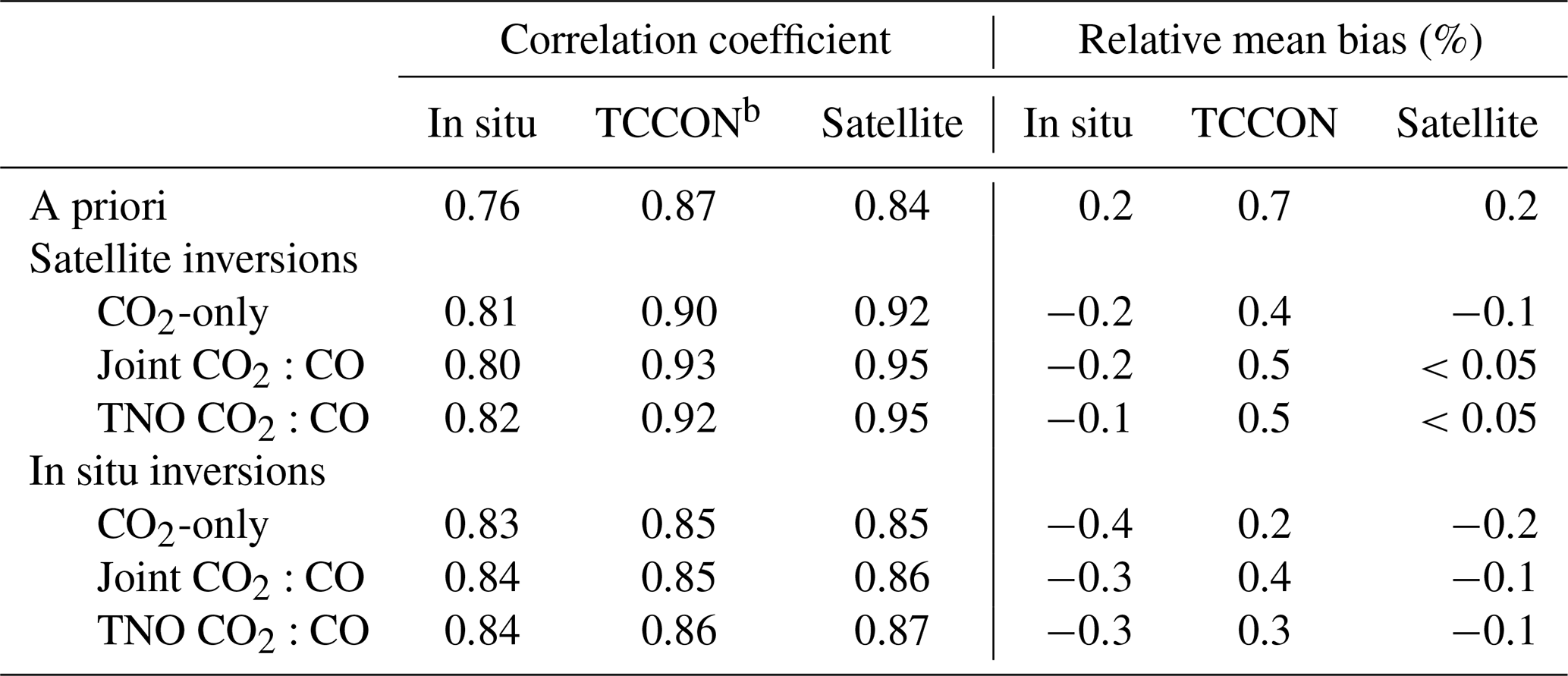
^a We use the Pearson correlation coefficient and relative mean bias (the means of the a posteriori and a priori difference divided by the a priori emission estimates) as measures of fit. ^b Five sites are within our domain (Fig. 2), including Bremen (Germany), Karlsruhe (Germany), Nicosia (Cyprus), Orléans (France), and Paris (France).

Table A2 Annual mean national CO₂ combustion emissions (Emis; Tg a⁻¹) and relative standard deviations (RSD; %) for 2018–2021 satellite inversions.

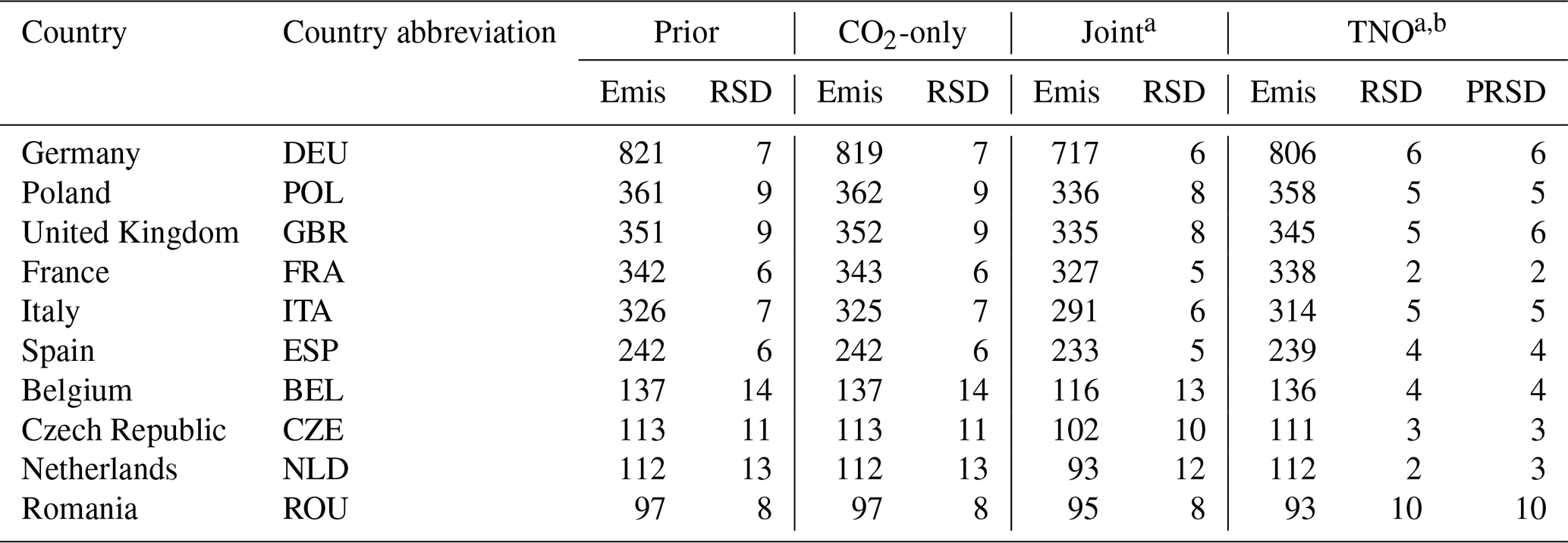
^a The satellite inversions that include CO only show means for July 2018–December 2021. ^b The a priori uncertainties for TNO differ from the CO₂-only and joint inversions, so we list the TNO a priori uncertainties (PRSD) as well. The higher a posteriori error for Romania is due to the error inflation factor used in the sequential inversion.

Table A3 Annual mean national CO₂ combustion emissions (Emis; Tg a⁻¹) and relative standard deviations (RSD; %) for 2018–2021 in situ inversions^a.

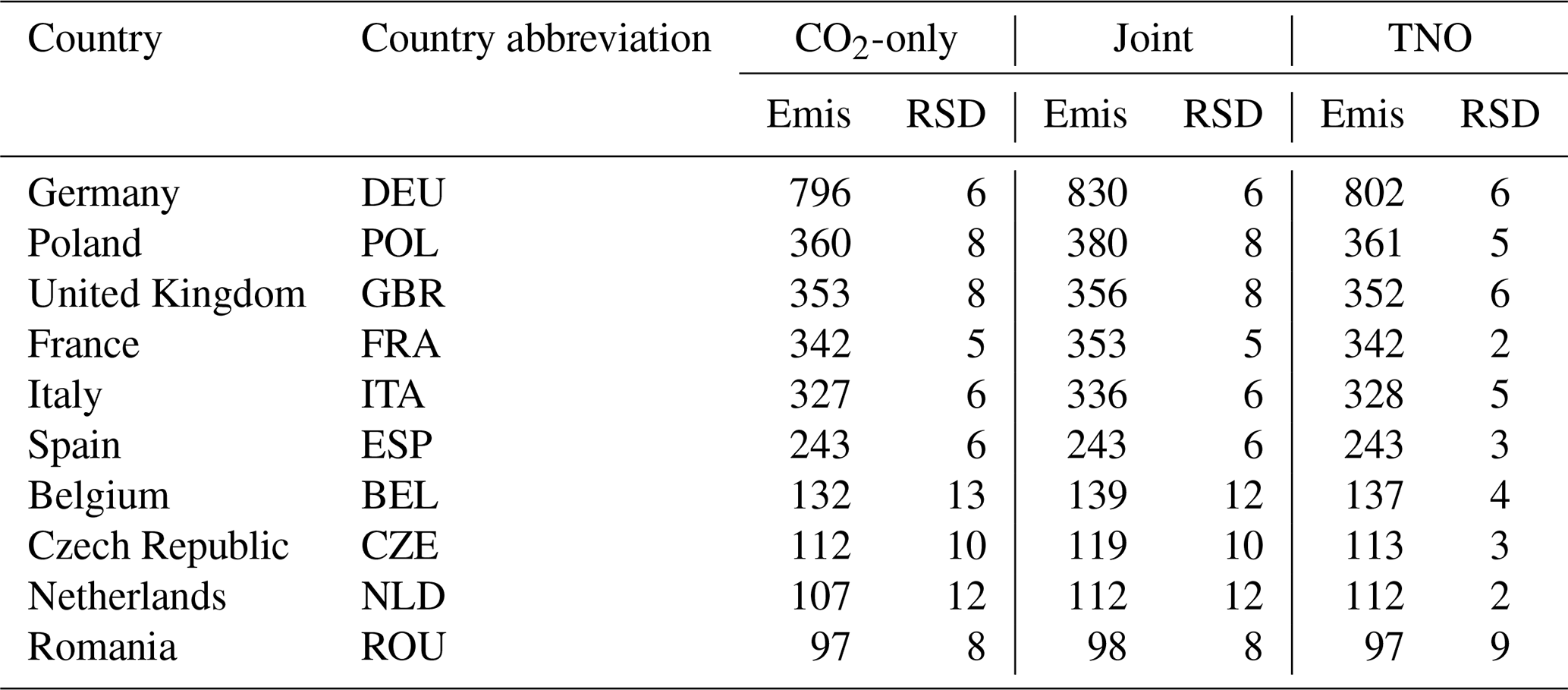
^a Only the a posteriori emissions are shown. The a priori emissions and uncertainties are listed in Table A2.

Table A4 Domain mean CO₂ non-combustion emissions for 2018–2021^a.

^a The non-combustion emissions include biogenic and non-combustion anthropogenic emission sources. ^b Joint and TNO inversion satellite results only include 2019–2021. The a priori non-combustion flux is the same for this period (−3.0 Gt a⁻¹).

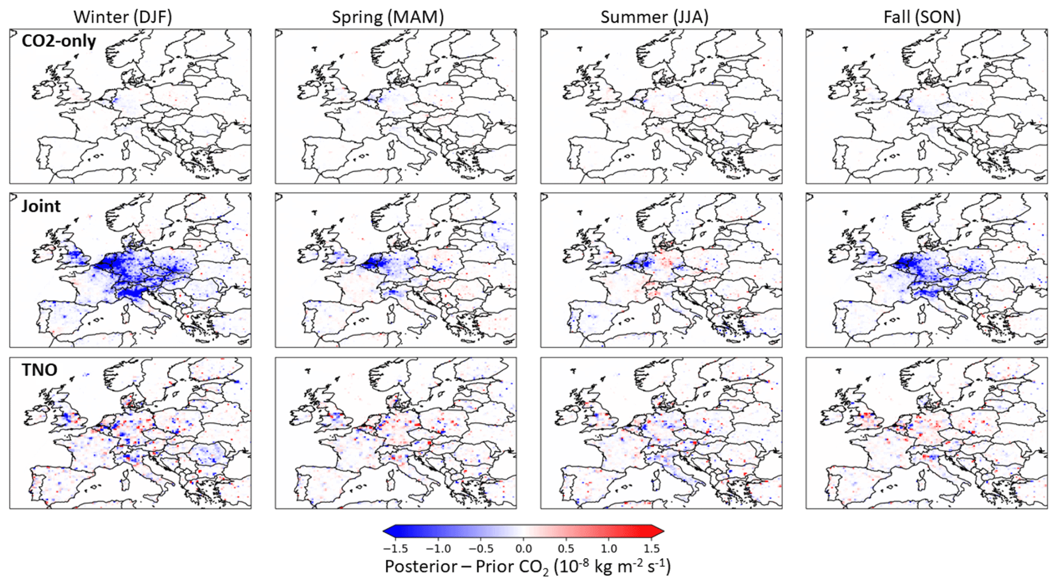
Figure A1 Seasonal mean a posteriori and a priori CO₂ combustion emissions difference for satellite inversions for 2018–2021. The inversions including CO satellite observations do not include emissions differences prior to July 2018.

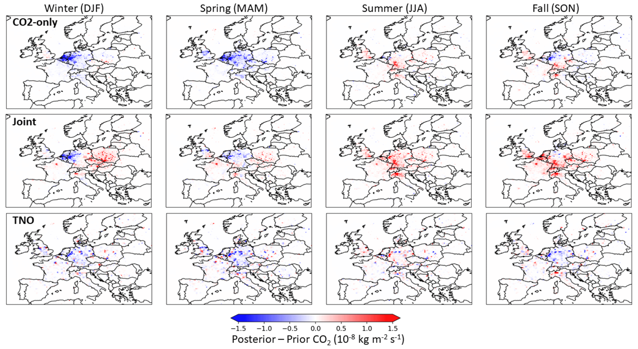
Figure A2 Same as Fig. A1 but for in situ inversions.

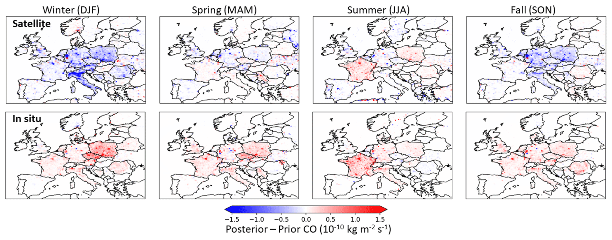
Figure A3 Same as Fig. A1 but for CO in satellite and in situ inversions.