the Creative Commons Attribution 4.0 License.
the Creative Commons Attribution 4.0 License.
 | 24 Jan 2024
Measurement report: Method for evaluating CO2 emissions from a cement plant using atmospheric δ(O2 ∕ N2) and CO2 measurements and its implication for future detection of CO2 capture signals
Kazuhiro Tsuboi
Hiroaki Kondo
Kentaro Ishijima
Nobuyuki Aoki
Hidekazu Matsueda
Kazuyuki Saito
Continuous observations of atmospheric and CO2 amount fractions have been carried out at Ryori (RYO), Japan, since August 2017. In these observations, the O2 : CO2 exchange ratio (ER, ) has frequently been lower than expected from short-term variations in emissions from terrestrial biospheric activities and combustion of liquid, gas, and solid fuels. This finding suggests a substantial effect of CO2 emissions from a cement plant located about 6 km northwest of RYO. To evaluate this effect quantitatively, we simulated CO2 amount fractions in the area around RYO by using a fine-scale atmospheric transport model that incorporated CO2 fluxes from terrestrial biospheric activities, fossil fuel combustion, and cement production. The simulated CO2 amount fractions were converted to O2 amount fractions by using the respective ER values of 1.1, 1.4, and 0 for the terrestrial biospheric activities, fossil fuel combustion, and cement production. Thus obtained O2 and CO2 amount fraction changes were used to derive a simulated ER for comparison with the observed ER. To extract the contribution of CO2 emissions from the cement plant, we used as an indicator variable, where is a conservative variable for terrestrial biospheric activities and fossil fuel combustion obtained by simultaneous analysis of observed and CO2 amount fractions and simulated ERs. We confirmed that the observed and simulated ER values and also the values and simulated CO2 amount fractions due only to cement production were generally consistent. These results suggest that combined measurements of and CO2 amount fractions will be useful for evaluating CO2 capture from flue gas at carbon capture and storage (CCS) plants, which, similar to a cement plant, change CO2 amount fractions without changing O2 values, although CCS plants differ from cement plants in the direction of CO2 exchange with the atmosphere.
- Article
(9616 KB) - Full-text XML
-
Supplement
(451 KB) - BibTeX
- EndNote


Simultaneous analysis of atmospheric and CO2 amount fractions has been used to estimate the global CO2 budget since the early 1990s (e.g., Keeling and Shertz, 1992). Recently, these analyses have also been applied to separate the contributions of different sources to the local CO2 budget in an urban area (e.g., Ishidoya et al., 2020; Sugawara et al., 2021; Pickers et al., 2022; Liu et al., 2023). This approach uses −O2 : CO2 exchange ratios (ER) or oxidative ratios (OR) () for terrestrial biospheric activities and fossil fuel combustion. Strictly speaking, there is a distinction between ERs and ORs; the ER refers to the exchange between the atmosphere and organisms or ecosystems while the OR indicates the stoichiometry of specific materials (Faassen et al., 2023). For terrestrial biospheric O2 and CO2 fluxes, ORs of 1.1 or 1.05 are generally used (Severinghaus, 1995; Resplandy et al., 2019), and for the fluxes due to fossil fuel combustion, ORs of 1.95 for gaseous fuels, 1.44 for oil and other liquid fuels, 1.17 for coal and other solid fuels, and 0 for cement production are typical (Keeling, 1988). Therefore, the atmospheric O2 amount fraction varies in opposite phase with the CO2 amount fraction, owing to terrestrial biospheric activities and fossil fuel combustion. The ORs are typically very stable, and the global average OR for fossil fuels is about 1.4 (e.g., Keeling and Manning, 2014).
In the cement production process, calcium carbonate is burned and calcium oxide and CO2 are produced as follows:
Because this chemical reaction emits CO2 to the atmosphere without O2 consumption, its OR is 0. It should be noted that the cement kilns are usually fired with fossil fuels, so that the overall ER for cement production is not 0. CO2 emissions from cement production account for about 2 % of global fossil fuel CO2 emissions (Friedlingstein et al., 2022). However, because it is difficult to separate the cement production signal from CO2 emissions due to fossil fuel combustion and terrestrial biospheric activities, no study has reported direct evidence of variations in the atmospheric CO2 amount fraction due to cement production at the Global Atmosphere Watch (GAW) program of the World Meteorological Organization (WMO) stations. In this context, simultaneous observations of and CO2 amount fractions are expected to be useful for separating out the cement production signal owing to its characteristic OR value. Moreover, Keeling et al. (2011), who examined the possibility of verifying rates of carbon capture and storage (CCS) and direct air capture of CO2 (DAC) by using changes in the atmospheric constituents, suggested that combined measurements of the and CO2 could powerfully constrain estimated rates.
To investigate CO2 leak detection from a CCS site, van Leeuwen and Meijer (2015) observed and CO2 from a 6 m tall mast that was 5–15 m away from artificial CO2 release points. They estimated that their measurement system could detect a CO2 leak of 103 t a−1 at a location up to 500 m away from the leak point. Pak et al. (2016) monitored the air for CO2 plumes at locations between 1 and 100 m from an artificial CO2 release point, and collected air samples typically between 9 and 20 m from the point where the CO2 amount fraction was 100–600 µmol mol−1 above ambient. They then analyzed the air samples for O2 and CO2 amount fractions and found much lower ERs than those expected from fossil fuel combustion and terrestrial biospheric activities. These studies support the suggestion by Keeling et al. (2011) regarding the usefulness of and CO2 measurements. As the next step to verify the usefulness of combined measurements of and CO2, their applicability to the detection of not only CO2 leaks but also CO2 capture from flue gas should be examined. In this regard, CCS/DAC plants remove CO2 from the atmosphere without causing any O2 changes, just as cement plants do, differing only in the direction of CO2 exchange between the plant and the atmosphere. Therefore, it should be possible to evaluate the ability of combined measurements to detect a CO2 capture signal by showing that they can be used to detect a cement production signal.
In this paper, we present evidence of the successful detection of a cement production signal by combined measurements of and CO2 at a ground station (a designated WMO/GAW local site) located near a cement plant. We also examine the usefulness of the measurements for future detection of CCS/DAC signals by using a fine-scale 3-D atmospheric transport model to investigate the consistency between the observed signal and the simulated CO2 emissions from the plant.
2.1 Observations of atmospheric δ(O N2) and CO2 amount fractions
Atmospheric and CO2 amount fractions have been observed continuously at the coastal station Ryori (RYO: 39∘2′ N, 141∘49′ E, 260 m a.s.l.; Fig. 1), Japan, since 2017, by using a paramagnetic O2 analyzer (POM-6E, Japan Air Liquid) and a non-dispersive infrared CO2 analyzer (NDIR; LI-7000, LI-COR), respectively. RYO is a designated WMO/GAW station, and the Japan Meteorological Agency (JMA) has also observed CO2, CH4, and CO amount fractions there since 1987, 1991, and 1991, respectively (e.g., Wada et al., 2011). The CO2, CH4, and CO amount fraction data observed by JMA are available online at the WMO World Data Centre for Greenhouse Gases (WMO/WDCGG; https://gaw.kishou.go.jp/, last access: 10 November 2023). A cement plant (Taiheiyo Cement Ofunato Plant) is 6 km away from RYO (Fig. 1). It should be noted that the CO2 amount fraction data posted on WDCGG have already been classified into the data for background air and those affected by local fossil fuel combustion including the cement production discussed in this study. The annual cement production at the plant is 1.966 × 10⁶ t a−1 (https://www.taiheiyo-cement.co.jp/english/index.html, 5 January 2024).
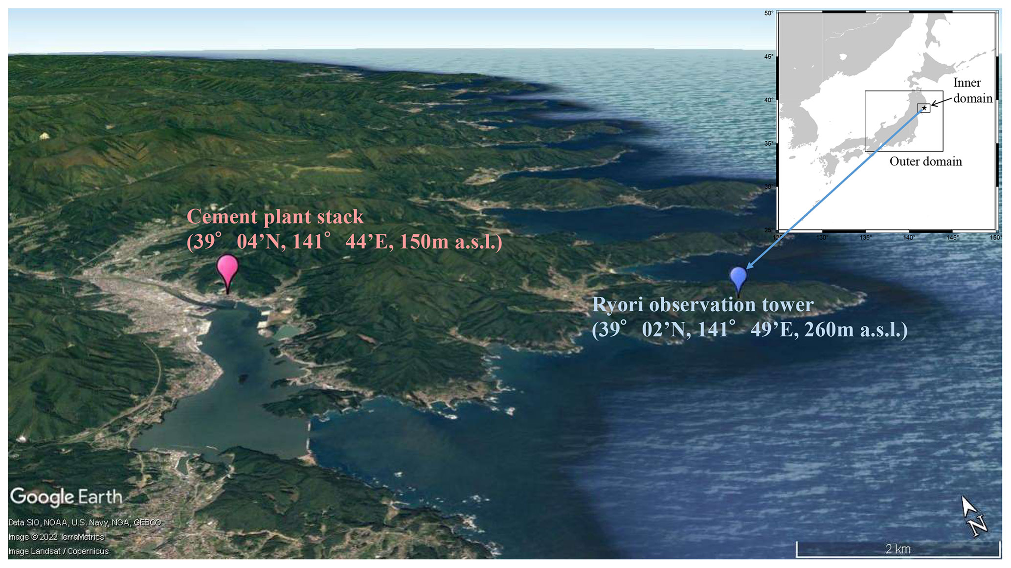
Figure 1Location of the Ryori site (RYO) and the cement plant on an aerial photograph from © Google Earth. The cement plant is about 6 km northwest of RYO. Inner and outer domains of the fine-scale 3-D atmospheric transport model (AIST-MM) used in the present study are also shown.
The is reported in per meg, where 1 per meg is 0.001 ‰:
where the subscripts “sample” and “standard” indicate the sample air and the standard gas, respectively. Because the O2 amount fraction in dry air is 0.2093–0.2094 mol mol−1 (Tohjima et al., 2005; Aoki et al., 2019), the addition of 1 µmol of O2 to 1 mol of dry air increases by 4.8 per meg (). If CO2 is converted one-for-one into O2, it causes to increase by 4.8 per meg, which is equivalent to an increase of 1 µmol mol−1 of O2 for each 1 µmol mol−1 decrease in CO2. Therefore, observed relative changes in were converted to those in O2 amount fraction by multiplying by 0.2094 µmol mol−1 (per meg)−1.
In this study, of each air sample was measured with a paramagnetic analyzer using high- and low-span standard air of which had been measured against our primary standard air (Cylinder No. CRC00045; AIST-scale) using a mass spectrometer (Thermo Scientific Delta-V) (Ishidoya and Murayama, 2014). The scale based on the primary standard air is our original scale, called the “EMRI/AIST scale” in Aoki et al. (2021). Sample air was taken at the tower heights of 20 m using a diaphragm pump at a flow rate higher than 10 L min−1 to prevent thermally diffusive fractionation of air molecules at the air intake (Blaine et al., 2006). The tower is situated on the windward side of the prevailing wind direction, and the surface below the tower consists of short grass. Then, a large portion of the air is exhausted from the buffer, with the remaining air allowed to flow into the analyzers from the center of the buffer. It is then sent to an electric cooling unit with a water trap cooled to −80 ∘C at a flow rate of 100 mL min−1, with the pressure stabilized to 0.1 Pa and measured for 90 min. After the measurements, high-span standard gas, prepared by adding appropriate amounts of pure O2 or N2 to industrially prepared CO2 standard air, was introduced into the analyzers with the same flow rate and pressure as the sample air and measured for 5 min, and low-span standard gas was then measured through the same procedure. The dilution effects on the O2 mole fraction measured by the paramagnetic analyzer were corrected experimentally, not only for the changes in CO2 of the sample air or standard gas measured by the NDIR, but also for the changes in Ar of the standard gas measured by the mass spectrometer as .
The analytical reproducibility of the and CO2 amount fraction measurements by the system was determined by repeated measurements of standard gas and found to be about 5 per meg and 0.06 µmol mol−1, respectively, for 2 min-average values. For more information, see Ishidoya et al. (2017). In this study, we use about 70 min-average mean values for analysis. It should be noted that gaps in the data seen at the end of August to beginning of September 2017 are due to maintenance and technical issues other than routine calibrations described earlier. The number of (and CO2 amount fraction) data points shown in Fig. 2 is 9220. Note that we used a mass spectrometer to measure both and the CO2 amount fraction of the working standard air, whereas we determined the CO2 amount fraction on the TU-10 scale using a gravimetrically prepared air-based CO2 standard gas system (Nakazawa et al., 1997). However, we found that the CO2 amount fractions observed in this study were systematically higher by about 1 µmol mol−1 than those observed by JMA and reported on the WMO scale (X2007), which is larger than that expected from the scale difference of about 0.2 µmol mol−1 between the TU-10 and WMO scales (Tsuboi et al., 2016). This discrepancy might be related to the LI-7000 NDIR used in this study because no significant difference has been found between the TU-10 and WMO scales at Minamitorishima, where a different NDIR (LI-820, LI-COR) has been used for continuous measurements of and CO2 amount fractions (Ishidoya et al., 2017). However, we found no significant difference in span sensitivities between the CO2 amount fractions observed in this study and those observed by JMA. Therefore, the systematic difference between the observed CO2 amount fractions and those observed by JMA does not affect the ER values, discussed in Sect. 3, which were calculated from changes in O2 and CO2 amount fractions. The and CO2 amount fractions observed at RYO are available in the Supplement.
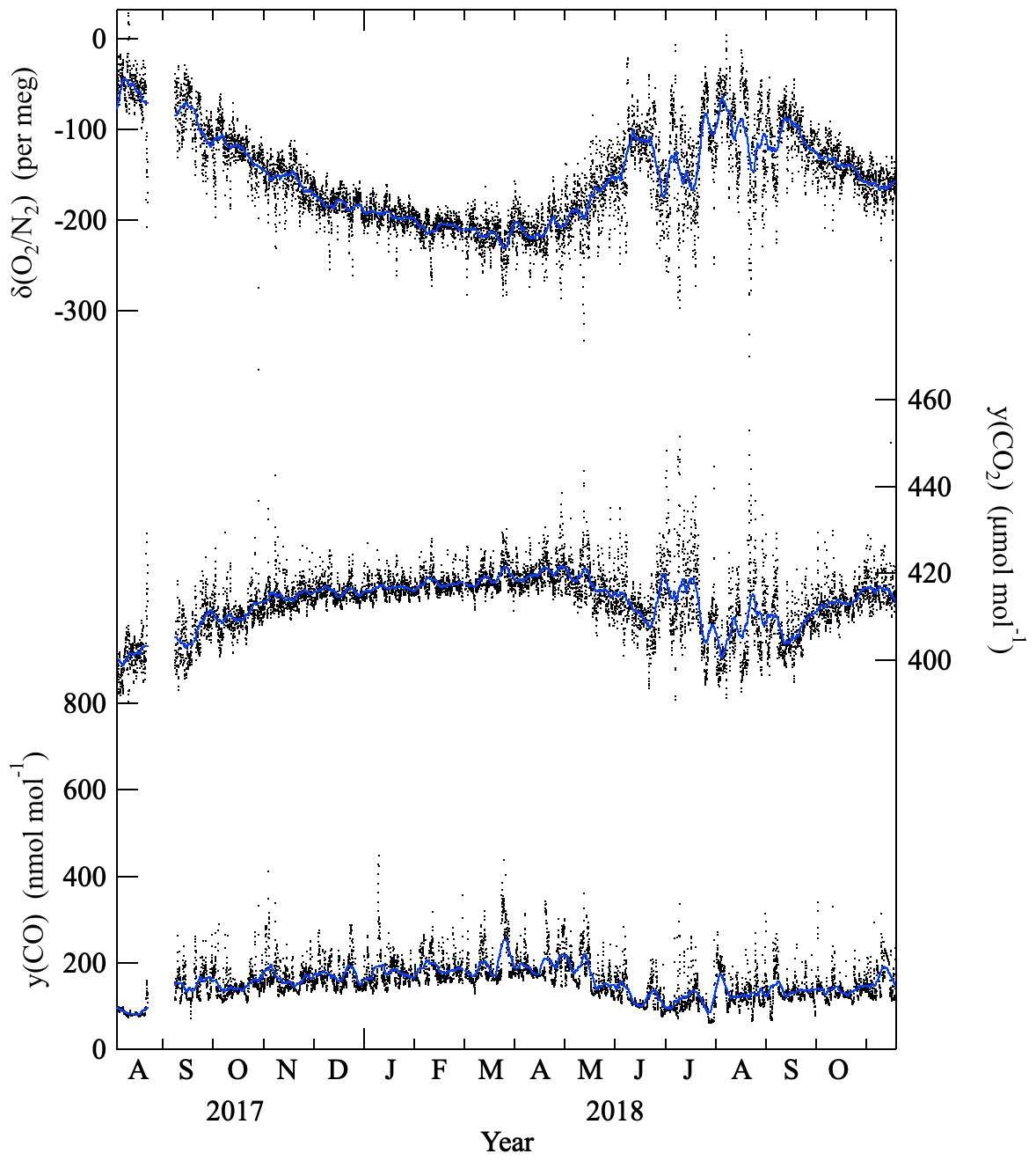
Figure 2 and CO2 and CO amount fractions (black dots) and their 1-week rolling average values (blue lines) observed at Ryori (RYO), Japan, from August 2017 to November 2018. and CO2 y axes are scaled to be visually comparable.
2.2 Simulation of atmospheric CO2 and O2 amount fractions using an atmospheric transport model
To calculate the local transport of CO2 around RYO, we used the National Institute of Advanced Industrial Science and Technology (AIST) Mesoscale Model (AIST-MM) fine-scale regional atmospheric transport model (Kondo et al., 2001). AIST-MM is a one-way nested model with an outer domain that covers east Japan with an approximately 10 km grid interval and an inner domain that covers an area of 120 km × 120 km near RYO with a grid interval of approximately 1 km (Fig. 1). The EAGrid2010-Japan emissions inventory (Fukui et al., 2014), an update of the EAGrid2000-Japan inventory (Kannari et al., 2007) to the year 2010, was used for fossil fuel combustion. In this study, fossil fuel combustion means anthropogenic CO2 sources other than cement production. The spatial resolution of EAGrid2010-Japan is approximately 1 km, and the temporal resolution is monthly average of 1 h. No further inter-annual correction of emissions is employed, but EAGrid2010-Japan considers the difference in traffic volume between weekdays and holidays. To calculate the CO2 budget for vegetation, the NCAR Land Surface Model (Bonan, 1996) was used as a sub-model, replacing the simple function of temperature and solar insolation used in the original AIST-MM for this calculation. The cement plant source was set at the location of the plant's stack, at the effective stack height of 275 m. The CO2 emissions from the cement plant were estimated from the clinker production capacity of the Ofunato plant in 2018 (Japan Cement Association, 2020). The clinker is a solid material produced in cement manufacture as an intermediary product of Portland cement, mainly consisting of CaO, SiO2, Al2O3, and Fe2O3. The annual emissions were calculated using the method of the Ministry of Environmental Protection (https://www.env.go.jp/earth/ondanka/ghg-mrv/methodology/material/methodology_2A1.pdf, last access: 5 January 2024, in Japanese) as
where E is the annual emissions of CO2 from the cement plant (t a−1), P is the annual production capacity of the clinker at the cement plant (t a−1), F is the CO2-to-clinker mass ratio of 0.516, and D is the cement kiln dust of 1. For initial and boundary conditions, we used GPV/MSM (grid point value of meso-scale model) meteorological data of wind, temperature, and humidity from JMA (https://www.jma.go.jp/jma/en/Activities/nwp.html, last access: 5 January 2024). As a result, CO2 amount fractions at RYO are calculated by summing up the contributions of the CO2 amount fraction for fossil fuel combustion, terrestrial biospheric activities, and cement production. In this study, not only CO2 amount fractions but also ERs are compared between the observed and simulated data. For this purpose, O2 amount fractions are calculated by summing up the respective contributions of CO2 amount fractions for fossil fuel combustion, terrestrial biospheric activities, and cement production multiplied by the −OR values of −1.4, −1.1, and 0. Here the 1.4 and 1.1 are typical ORs for fossil fuel combustion and terrestrial biospheric activities, respectively. For comparison, we also calculate ER values for the O2 and CO2 amount fractions simulated without including the contribution of cement production. In this regard, it should be noted that Faassen et al. (2023) carried out continuous observations of and the CO2 amount fraction at a forest site in Finland, and they found higher ER (referred to as “ERatmos” in their study) than 2.0 during the morning transition for the average diurnal cycle in summer. Such high ER cannot be obtained from summing up the contributions of fossil fuel combustion and terrestrial biospheric activities at the surface, and therefore they suggested the ER signal not only represents the diurnal cycle of the forest exchange but also includes other factors, including entrainment of air masses in the atmospheric boundary layer before midday, with different thermodynamic and atmospheric composition characteristics. Considering their results, we examined average diurnal cycles of and the CO2 amount fraction at RYO in October 2017 and August 2018 (Fig. A1a–d in Appendix A). We found the ER values are close to 1 throughout the day both for the observed and simulated diurnal cycles. Therefore, we consider the entrainment of air masses does not change the ER at RYO substantially, and the atmospheric transport processes in the AIST-MM are appropriate for comparing the observational results in the present study. The CO2 amount fractions for fossil fuel combustion, terrestrial biospheric activities, and cement production calculated by the AIST-MM are available in the Supplement.
2.3 Extraction of a cement signal from the observed data
We extract signals of cement production based on the simultaneous measurements of and CO2 amount fractions. For this purpose, we use as an indicator:
where X(O2) (= 0.2094) is the fraction of atmospheric O2, and αB+F is the expected ER for terrestrial biospheric activities and fossil fuel combustion. The is closely related to atmospheric potential oxygen (δ(APO)), which is conserved for terrestrial biospheric activities (Stephens et al., 1998). Here, y stands for the dry amount fraction of gas, as recommended by the IUPAC Green Book (Cohen et al., 2007). In our previous study, we calculated δ(APO) as
where 2000 is an arbitrary reference (Ishidoya et al., 2022). For αB+F values, we use monthly average ER values calculated from the simulated O2 and CO2 values without considering the contribution of cement production (dotted black line in Fig. 5, bottom, discussed below). If there are no substantial contributions from air–sea O2 and CO2 exchanges, then indicates the change in the atmospheric CO2 amount fraction due only to cement production. No air–sea exchanges can be assumed if the wind field, surface ocean biological production, and ocean temperature are constant throughout the month. In fact, day-to-day variations in due to the contribution of oceanic signal cannot be ignorable within a month as reported in previous studies (e.g., Goto et al., 2017). However, as shown in Figs. 5 and 6 here, variations in the CO2 amount fraction due to cement production occurred over periods of less than 1 d. Taking these findings into consideration, we derived the baseline variation in , which does not include a substantial contribution from cement production, as follows. First, we calculated the standard deviation (1σ) of each value from the 24 h running means of . Then, we removed values greater than the 24 h running mean of from the analysis. Finally, we recalculated the 24 h running means by using the residual values, and regarded them as the baseline variation. Accordingly, the anomaly obtained by subtracting the baseline variation from each value is considered to indicate CO2 changes due mainly to the contribution of the cement production.
From August 2017 to November 2018, and CO2 amount fractions observed at RYO varied cyclically in opposite phase to each other on timescales from several hours to seasons (Fig. 2); however, variations in CO2 and CO amount fractions were roughly in phase. The opposite-phase variations of and CO2 amount fractions were driven by fossil fuel combustion and terrestrial biospheric activities. By contrast, the atmospheric O2 variation (µmol mol−1) due to the air–sea exchange of O2 is much larger than that of CO2 on timescales shorter than 1 year because of the difference in their equilibration times between the atmosphere and the surface ocean: the equilibration time for O2 is about 1 month and for CO2 it is about 1 year because of the carbonate dissociation effect on the air–sea exchange of CO2 (Keeling et al., 1993). The in-phase variations of the CO2 and CO amount fractions were also driven by fossil fuel combustion and biomass burning. CO : CO2 ratios for fossil fuel combustion and biomass burning reported by previous studies are about 0.01–0.04 and > 0.1, respectively (e.g., Nara et al., 2011; Tohjima et al., 2014; Niwa et al., 2014). The short-term (several hours to several days) variations in CO : CO2 ratios were about 0.01 from late autumn to early spring, but they were much smaller in summer (Fig. 2). These results suggest, therefore, that the short-term variations in and CO2 amount fractions were driven mainly by fossil fuel combustion in winter and mainly by terrestrial biospheric activities in summer. Over 1 year of measurements CO amount fractions also showed a seasonal cycle with a summertime minimum that is attributed to the air mass around Japan: in winter the air mass is of continental origin and in summer it is of marine origin.
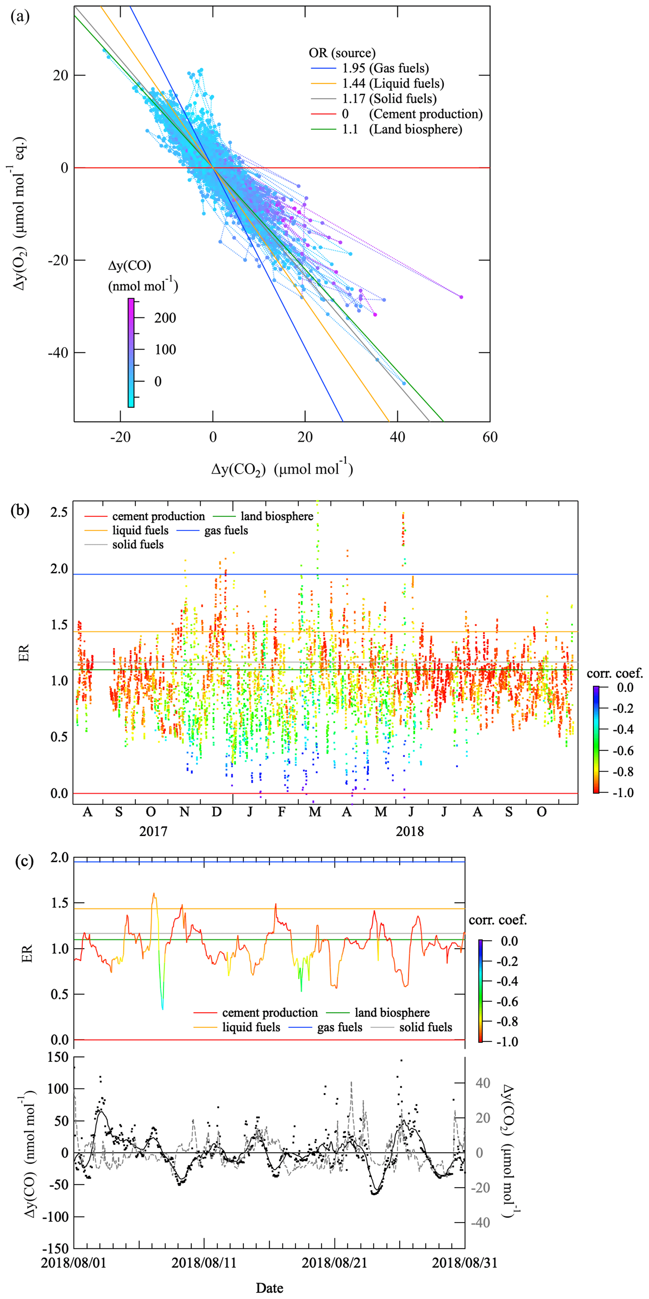
Figure 3(a) Relationship between Δy(O2) and Δy(CO2) at RYO from August 2017 to November 2018. Δy(O2), Δy(CO2), and Δy(CO) were calculated by subtracting the 1-week mean values of , CO2, and CO amount fractions from their observed values; then values were converted to the equivalent Δy(O2). Δy(CO) values are shown by the color scale. The plotted ER values are from Keeling (1988) and Severinghaus (1995). (b) ER values calculated by least-squares fitting of regression lines to the observed Δy(O2) and Δy(CO2) values shown in (a) during successive 24 h periods (before and after 12 h of each point) throughout the observation period. (c) Same ER as in (b) but for August 2018. Δy(CO) (black dots) and its 24 h averages (solid black line), and Δy(CO2) (dashed gray line) are also shown.
In this study, we focused on the short-term variations in and the CO2 and CO amount fractions (Fig. 2) to extract local effects of cement production. Therefore, we subtracted 1-week rolling average values of and the CO2 and CO amount fractions from the observed values to exclude their baseline variations, and examined the relationships among the residuals (Δy(O2), Δy(CO2), and Δy(CO); Fig. 3a). Here, Δy(O2) is the equivalent value in µmol mol−1 converted from . We also plotted the ER values calculated by least-squares fitting of regression lines to the observed Δy(O2) and Δy(CO2) values during successive 24 h periods in Fig. 3b. As seen in the figure, both ER values higher and lower than 1.1 were observed throughout the observation periods. When the terrestrial biosphere emits CO2 to the atmosphere, i.e., the respiration signal is larger than the photosynthesis signal, ER values ranging from 1.05 to 2.00 are expected from combination fluxes of terrestrial biospheric activities, gas, liquid, and solid fuels combustion. Similar ER values have been observed at other Japanese sites (e.g., Minejima et al., 2012; Goto et al., 2013; Ishidoya et al., 2020).
On the other hand, when the photosynthesis signal is larger than the respiration signal, ER values for the combination fluxes could be variable and potentially even lower than 1.05. Therefore, we consider that the observed low ER values with high Δy(CO) and Δy(CO2) are attributed to substantial CO2 flux from cement production, of which the ER value is 0, rather than the photosynthesis signal. These characteristics can be seen from the typical ER, Δy(CO), and Δy(CO2) in August 2018 plotted in Fig. 3c. Therefore, it is considered that air mass having ER values lower than 1.05 and Δy(CO) and Δy(CO2) higher than 0 simultaneously indicates CO2 flux from cement production mixes with the surrounding air that has already been influenced by terrestrial biospheric activities or fossil fuels combustion. Similar characteristic relationships have previously been observed only in artificial CO2 release experiments of which the OR value is 0, such as those described by van Leeuwen and Meijer (2015) and Pak et al. (2016). Therefore, we used the AIST-MM model to calculate atmospheric CO2 amount fractions, with or without taking into account the CO2 flux from the cement plant near RYO, and to convert the calculated CO2 amount fractions to O2 amount fractions using the respective OR values of fossil fuels and terrestrial biospheric activities. Then we compared the observed and simulated ER values. Figure 4 shows examples of the performance of the AIST-MM in the present calculation. Figure 4a shows the monthly average of hourly CO2 amount fractions is slightly overestimated at night and underestimated in the daytime except for February; however, the absolute value of the difference is less than 2 µmol mol−1 in most case. Figure 4b is a scatter plot of the difference from 391.14 µmol mol−1 (the minimum concentration of observed CO2 in the 7 months) between the calculated and observed concentration for all the hourly data in the 7 months. The FAC2 (fraction of calculations within a factor 2 of observations) is 0.976, where the model acceptance criterion of FAC2 is greater than 0.5 (Hanna and Chang, 2012), and Pearson's correlation coefficient is 0.69. The discrepancies between the observed and simulated values can be attributed to the limited resolution of the model in the complex terrain, or to problems in the parameterization of transport processes or in the CO2 sources/sinks incorporated into the AIST-MM.
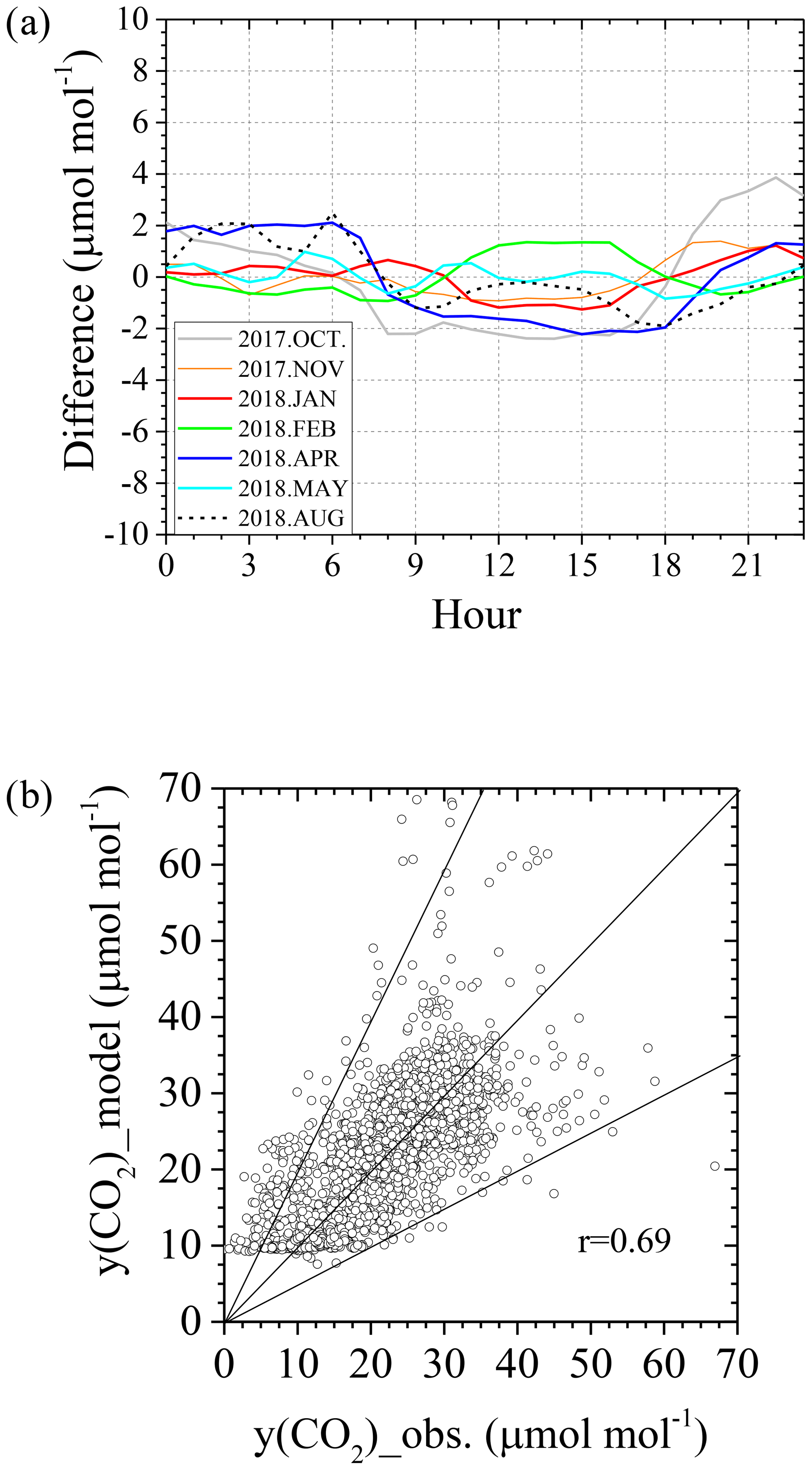
Figure 4(a) Difference of monthly average of hourly amount fraction of CO2 between calculated and observed concentration at RYO. (b) Scatter plot between observed and calculated CO2 amount fraction deviation for all the hourly data of 7 months at RYO. 391.14 µmol mol−1 (the minimum value of observed CO2 amount fraction in 7 months) was subtracted from both of the data groups. Straight lines indicate the range of FAC2.
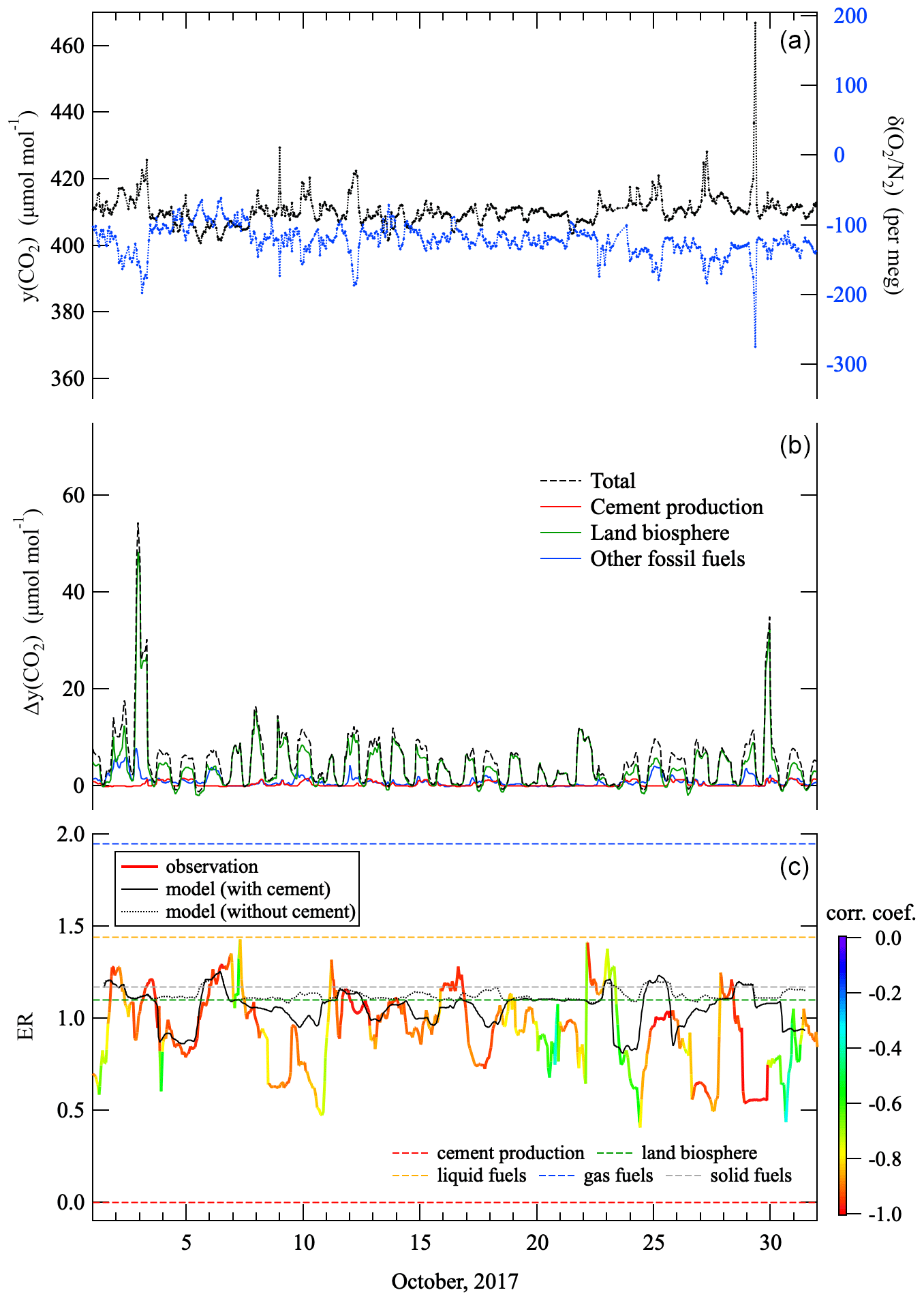
Figure 5(a) Variations in CO2 amount fractions and observed at RYO in October 2017. (b) Variations in the total CO2 amount fraction simulated by the AIST-MM (dashed black line, see text), and the contributions of CO2 amount fraction for cement production (solid red line), terrestrial biospheric activities (solid green line), and fossil fuel consumption other than cement production (solid blue line). The simulated CO2 amount fractions were calculated from the sources and sinks in east Japan with no background amount fraction, i.e., Δ denotes deviations from the background amount fraction. (c) Variations in ER calculated by least-squares fitting of regression lines to the observed and CO2 values during successive 24 h periods (thick colored line, where the line color indicates the value of the correlation coefficient). The corresponding ER values calculated from the simulated O2 and CO2 amount fractions by the AIST-MM with and without considering the amount fraction of cement production are shown by solid and dotted black lines, respectively. Dashed horizontal lines show the expected OR values for the consumption of gas, liquid, and solid fuels (Keeling, 1988); terrestrial biospheric activities (Severinghaus, 1995); and cement production.
In October 2017, short-term variations in observed CO2 and were opposite in phase, and the amplitudes (in µmol mol−1) of some CO2 variations were larger than those of the corresponding variations (Fig. 5). If the short-term variations were driven by terrestrial biospheric activities and the consumption of gas, liquid, and solid fuels, then the amplitudes of CO2 should be smaller than those of the . Therefore, this result suggests an effect of cement production is superimposed on fossil fuel combustion and/or terrestrial biospheric activities. Similar characteristic variations suggesting a cement production effect were also seen in the observations made at RYO in November 2017 and in January, February, April, May, and August 2018 as presented in Appendix B. The simulated CO2 amount fraction, calculated from the sources and sinks in east Japan with no background amount fraction by the AIST-MM, is also shown in Fig. 5. The contribution of the CO2 amount fraction for the three components (cement production, terrestrial biospheric activities, and fossil fuel consumption other than cement production) is also shown in Fig. 5. The results demonstrate that cement production contributed substantially to the simulated CO2 amount fraction. We examined the effect of cement production on ER values by calculating ER values by fitting regression lines to the observed and simulated O2 and CO2 amount fractions during successive 24 h periods (Fig. 5, bottom). Both the observed ER values and those simulated are frequently lower than 1.1, while the ER values simulated without including cement production show lower values than 1.1 occasionally (Figs. 5 and B1a–f in Appendix B). Therefore, CO2 emissions from the cement plant must be incorporated into the transport model to reproduce the detailed variations in atmospheric O2 and CO2 amount fractions at RYO.
Next, we extracted signals of cement production based on calculated from the simultaneous measurements of and CO2 amount fractions (see details in Sect. 2.3). In October 2017, the and CO amount fraction maxima at RYO appeared at the same time that the wind was blowing from the northwest (most frequently over the range of 270–300∘) (https://www.data.jma.go.jp/env/data/report/data/download/atm_bg_e.html, last access: 24 August 2021) (Fig. 6). This result suggests that the short-term variations in were driven mainly by air masses transported from the cement plant, which is about 6 km northwest of RYO. These findings also indicate that it is possible to extract CO2 amount fraction data from background air at RYO by selecting observed ER and CO amount fraction data. We have confirmed that the present method of JMA used to select background air for the data posted on WDCGG is sufficient to exclude the effect of cement production; nevertheless, the use of ER may provide an additional constraint. Note that CO is emitted during fossil fuel combustion at the cement plant to supply electricity and heat for cement production. This means CO2 is presumably released as well, so that the overall ER for the CO2 emitted from cement plant (cement production + fossil fuel combustion) would not be 0.
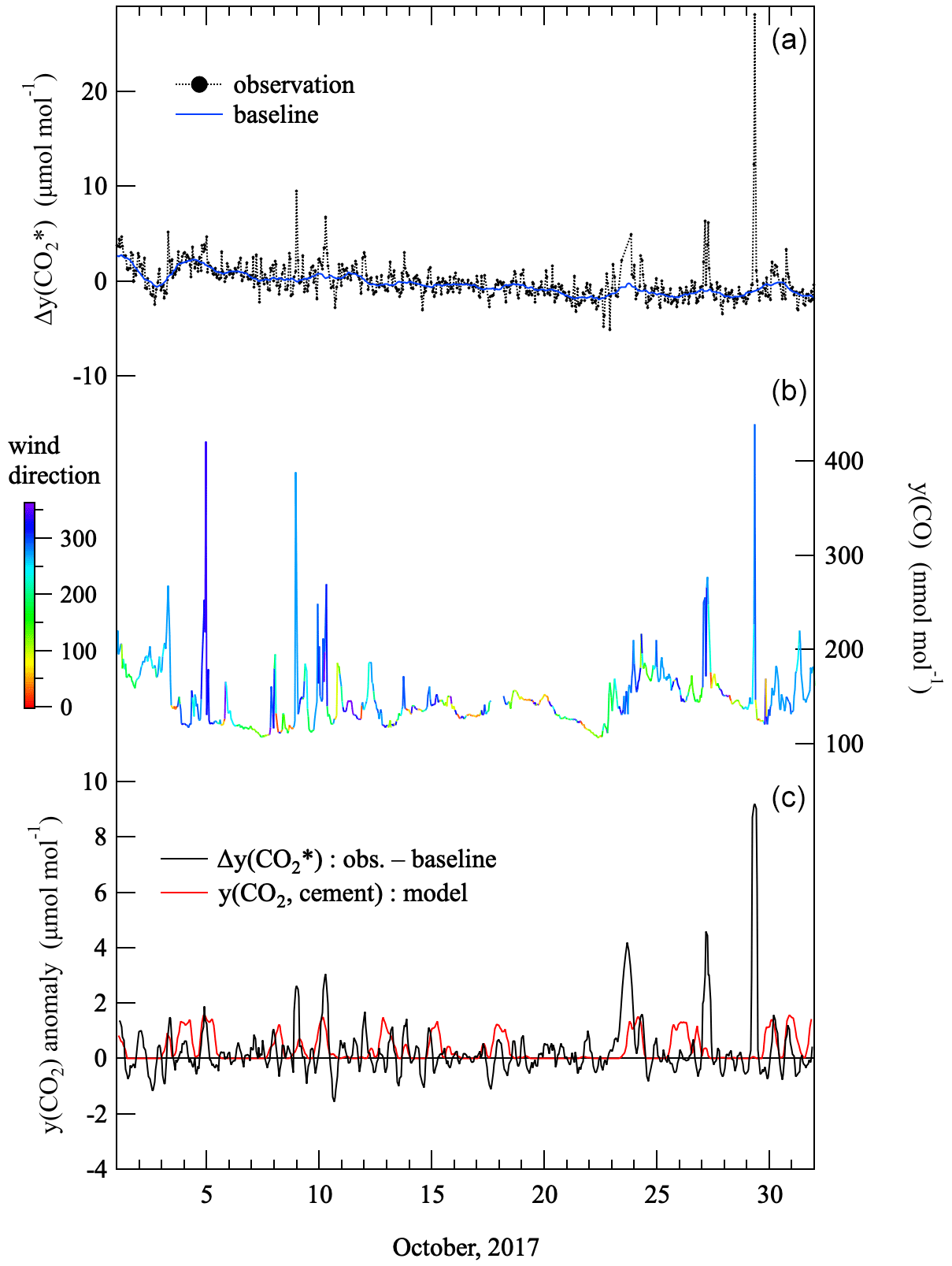
Figure 6(a) Variations in calculated from the observed CO2 amount fractions and (filled black circles) in October 2017, and the baseline variation (solid blue line). Δ denotes deviations from their monthly mean values. See text for the definition of and the method used to obtain the baseline variation. (b) Variations in CO amount fractions in October 2017 and the simultaneously observed wind direction (in degrees). (c) 5 h-average anomalies from the baseline variation and the corresponding variation in the CO2 amount fraction due only to cement production (y(CO2,cement)) simulated by the AIST-MM (same as the red line in the middle part of Fig. 4).
To examine the consistency between the observed and simulated CO2 emissions from the cement plant, we compared 5 h means of anomalies with changes in the CO2 amount fraction due to the contribution of cement production as simulated by the AIST-MM (hereafter referred to as “y(CO2,cement)”) (Fig. 6, bottom). The result shows that variations in the anomaly and y(CO2,cement) are of the same order of magnitude, although they do not necessarily occur simultaneously. This result suggests that we succeeded in using to detect a signal of CO2 emissions owing to the cement production, and that this signal can be used to validate a fine-scale atmospheric transport model. In this context, van Leeuwen and Meijer (2015) suggested that a CO2 leak of 103 t a−1 is detectable at a location up to 500 m away from the leak point based on their observations of atmospheric O2 and CO2 amount fractions. If this relationship follows an inverse square law, a CO2 leak of 1.44 × 10⁵ t a−1 should be detectable at locations up to 6 km from the leak point. Therefore, about 106 t a−1 of the CO2 emissions from the cement plant in this study, calculated with Eq. (2), is large enough to be detected at RYO. Features during November 2017, January, February, April, May, and August 2018 were similar (Fig. B2a–f in Appendix B), although the short-term variations in in May 2018 (Fig. B2e) were noisier than in the other months, probably because of an effect of short-term variations in the air–sea O2 flux due to high primary production during the spring bloom in the nearby coastal ocean (e.g., Yamagishi et al., 2008).
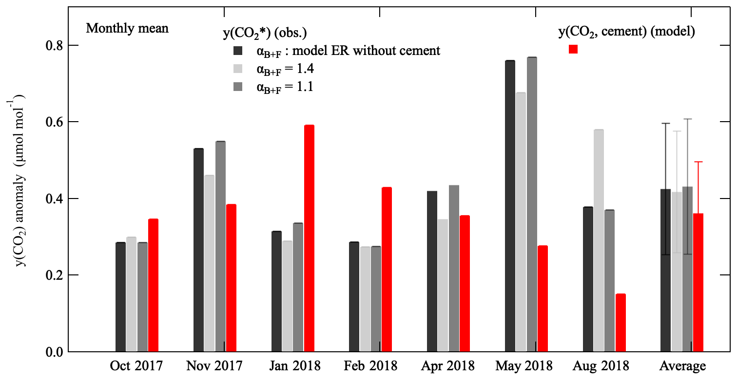
Figure 7Monthly means of anomalies, obtained using model-simulated αB+F values (as in Figs. 5 and B1a–f) and αB+F values of 1.4 and 1.1, and y(CO2,cement). The monthly mean values averaged over the 5 months are shown at the right. Error bars indicate monthly variability (±1σ).
The monthly mean anomalies shown in Fig. 7 were calculated using the ER (αB+F) value calculated by the AIST-MM for terrestrial biospheric activities and fossil fuel consumption excluding cement production. In Fig. 7, these anomaly values as well as those calculated using αB+F values of 1.4 and 1.1 are compared with monthly mean y(CO2,cement) values. The monthly mean anomalies were generally consistent with the monthly mean y(CO2,cement) values from October, November, February, and April, while those were smaller in January and larger in May and August. The discrepancy between the monthly mean anomaly and y(CO2,cement) is not explained by month-to-month changes in the cement production, since the production of clinker at the cement plant for each month was not markedly different from each other (Taiheiyo Cement Co., personal communication, 2022). We also confirmed that monthly mean y(CO2,cement) values were related to the occurrence of northwesterly winds (i.e., wind blowing from the cement plant). However, the average wind direction simulated by the AIST-MM when high y(CO2,cement) values appeared (around 300∘) was slightly but systematically different from that for observed wind direction (around 270∘) (Fig. B3a and b in Appendix B). This discrepancy is probably due to the underestimation of the altitude of Ryori ridge, which is located between the cement plant and the RYO site. Such an underestimation makes it easy to transport the CO2 emitted from the cement plant directly to RYO over the ridge since the cement plant is located around 300∘ from the RYO site. This is also consistent with the fact that the larger monthly mean y(CO2,cement) than the monthly mean anomalies are found in January and February when prevailing wind direction is northwesterly. The complex terrain around RYO such as the Ryori ridge would also contribute to the discrepancy between the monthly mean anomaly and y(CO2,cement) in May and August at least partly. In May, it is considered that an effect of the oceanic O2 flux on anomaly is also substantial, since we can distinguish short-term variations in without simultaneous changes in the CO2 amount fraction (Fig. B1e).
It was also found from Fig. 7 that the monthly mean anomaly did not depend on the αB+F value used to calculate , except August 2018. In addition, the average monthly mean anomaly values and the average y(CO2,cement) during the 7 months (right-hand side of Fig. 7) agreed within their monthly variabilities. These results suggest that it is not necessary to use the αB+F value simulated by the AIST-MM to estimate the contribution of cement production to the atmospheric CO2 amount fraction at RYO; rather, it can be estimated from only the observed by assuming an αB+F value of 1.1 or 1.4. This is also applicable on shorter timescales (Fig. B4a and b in Appendix B). Therefore, we can derive the observed at RYO without using any simulated value by an atmospheric transport model, and the observed can be used to validate hourly to annual average CO2 fluxes from cement production simulated by a fine-scale atmospheric transport model. It should also be noted that we did not use CO amount fraction for the calculation of . This is an important advantage to apply to detect CO2 capture and/or CO2 leak which does not emit CO.
is expected to be an indicator for detecting the signal of CO2 capture from flue gas at the cement plant. At a cement plant, CO2 is removed from flue gas without any O2 changes. Therefore, if the CO2 emitted during cement production, which is about 106 t a−1 at this plant, is removed from the flue gas, then the 7-month mean anomaly would change from 0.4 to 0 µmol mol−1. Thus, a cement plant can be a useful site not only for demonstrating carbon capture from flue gas but also for monitoring its efficiency based on combined measurements of and CO2. In addition, during the future operation of a large-scale DAC plant, a negative annual mean anomaly value should be observed because a DAC plant removes CO2 from the atmosphere without emitting O2 to the atmosphere.
We analyzed atmospheric and CO2 and CO amount fraction data observed continuously at RYO to extract a CO2 emissions signal from a cement plant located about 6 km northwest of RYO. The observed and CO2 amount fractions varied cyclically in opposite phase to each other on timescales from several hours to seasons. From the CO : CO2 ratios, the short-term variations in and CO2 amount fraction were inferred to be driven mainly by fossil fuel combustion in winter and by terrestrial biospheric activities in summer. We found that an ER lower than 1.1 was frequently associated with short-term variations, especially when the CO amount fraction was high; this result suggests a substantial effect of cement production, which has an ER of 0. We compared observed CO2 amount fractions with those simulated by the AIST-MM for October and November 2017 and January, February, April, May, and August 2018. FAC2 for the data throughout the observation period was 0.976, which was greater than the model acceptance criterion of 0.5. Therefore, the AIST-MM-reproduced general characteristics of the observed CO2 amount fraction were reproduced by the AIST-MM.
We calculated the simulated ER values by using simulated values obtained from simulated CO2 amount fractions and OR values of 1.1, 1.4, and 0 for terrestrial biospheric activities, fossil fuel combustion, and cement production, respectively. As in the observations, simulated ER values lower than 1.1 were frequently associated with short-term variations. was calculated from the observed and CO2 amount fractions and the simulated αB+F to extract the cement production signal. Variations in the anomaly relative to baseline values were generally of the same order of magnitude as the CO2 amount fraction changes due to the contribution of cement production simulated by the AIST-MM (y(CO2,cement)). The monthly mean anomaly averaged over the 7 months examined in this study and the 7-month average of y(CO2,cement) agreed within their variabilities.
These results confirm that monthly to annual average CO2 emissions from a cement plant can be detected by using , and, therefore, that a cement plant will be a useful site for demonstrating and monitoring CO2 capture from flue gas in the future. As a remaining topic, some of the more detailed variations in the CO2 amount fractions were not reproduced by the AIST-MM. This is at least partly due to the spatial resolution of the AIST-MM which limited its ability to reproduce air transport from a point source, such as the cement plant in the present study. In the future this work could be expanded on by using a higher-resolution atmospheric transport model to improve the agreement between the observed and simulated CO2 amount fractions. An additional step could be developing a more accurate method for extracting due only to cement production, especially for the period when air–sea O2 flux is substantial. This would improve the estimation of the amount of CO2 capture and/or CO2 leak around the observation site from an inversion analysis using the higher-resolution atmospheric transport model.
As we described in Sect. 2.2, Faassen et al. (2023) found higher ER values (“ERatmos” in their study) than 2.0 at a forest site in Finland during the morning transition for the average diurnal cycles of and the CO2 amount fraction in summer. On the other hand, Ishidoya et al. (2013) reported ER values (“ERatm” in their study) close to 1 at a Japanese forest site in summer, for the average diurnal cycles throughout the day. Considering the discrepancy between these values from Faassen et al. (2023) and Ishidoya et al. (2013), we derive the average diurnal cycle of and the CO2 amount fraction at RYO. For this purpose, deviations of and the CO2 amount fraction from their 24 h mean values were calculated, and the were converted to Δy(O2) by multiplying X(O2) (= 0.2094). Figure A1a–b show the average diurnal cycles of Δy(O2) and Δy(CO2) in October 2017, and their relationship. Those for August 2018 are also shown in Fig. A1c–d. As seen from the figures, the observed Δy(O2) took maxima in the daytime, and the ER values for the average diurnal cycles at RYO were close to 1 throughout the day. The corresponding diurnal Δy(O2) and Δy(CO2) cycles and their relationships obtained from the simulated results by the AIST-MM are also shown in Fig. A1a–d. Similar to the observations, it was found that the simulated Δy(O2) took maxima in the daytime and the ERs were close to 1 throughout the day. These facts indicate the observed ER at RYO can be reproduced by the AIST-MM generally, including the period during the morning transition. Therefore, an entrainment of air mass to yield high ER during the morning suggested by Faassen et al. (2023) may be a characteristic phenomenon at their observational site.
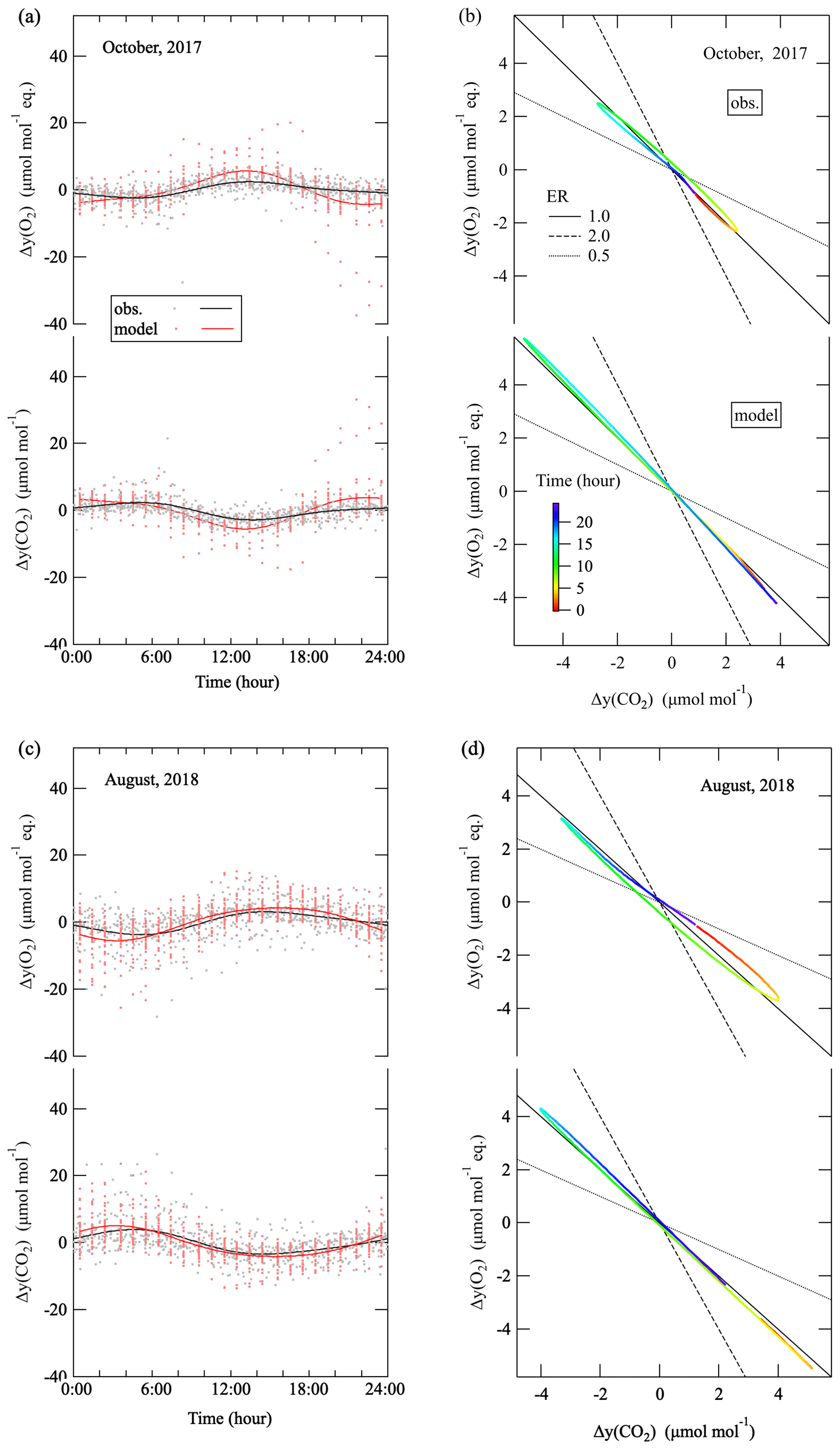
Figure A1(a) Average diurnal cycles of the observed Δy(O2) and Δy(CO2) (gray dots) in October 2017. Δ denotes deviations of and y(CO2) from their 24 h mean values. The was converted to Δy(O2) by multiplying X(O2) (= 0.2094). Best-fit curves to the data, represented by the fundamental and its first harmonics (periods of 24 and 12 h) terms, are also shown (black lines). Those of Δy(O2) and Δy(CO2) (red dots) and best-fit curves (red lines) simulated by the AIST-MM are also shown. (b) Relationships between the best-fit curves of the observed (top panel) and simulated (bottom panel) Δy(O2) and Δy(CO2) shown in (a). The color scale denotes the time of the day. The relationships expected from the ER of 1.0, 2.0, and 0.5 are also shown by solid, dashed, and dotted black lines, respectively. (c) Same as in (a) but for August 2018. (d) Same as in (b) but for August 2018.
In the main text, variations in CO2 amount fractions and observed at RYO, CO2 amount fractions simulated by the AIST-MM, and ERs calculated from the observed and simulated data in October 2017 are shown in Fig. 5. We also show the corresponding figures in November 2017 and in January, February, April, May, and August 2018 in Fig. B1a, b, c, d, e, and f, respectively. Variations in , CO amount fractions in October 2017, and 5 h averages of the anomalies from the baseline variation and those of y(CO2,cement) simulated by the AIST-MM are shown in Fig. 6. We also show the corresponding figures in November 2017 and in January, February, April, May, and August 2018 in Fig. B2a, b, c, d, e, and f, respectively. General characteristics of Figs. B1a–f and B2a–f are found to be similar to those discussed in the main text for Figs. 5 and 6, respectively. However, we can distinguish short-term variations in without simultaneous changes in the CO2 amount fraction in May 2018 (Fig. B1e), which may be attributed to substantial oceanic O2 flux due to high primary production during the spring bloom.
Figure B3a shows relationships between and wind direction at RYO. Same as in Fig. B3a but for y(CO2,cement) simulated by the AIST-MM is shown in Fig. B3b. The average wind direction when high y(CO2,cement) values appeared is around 300∘, while that for observed wind direction is around 270∘. This discrepancy is probably due to insufficient spatial resolution of the AIST-MM as discussed in the main text.
Figure B4a and b show the bottom panels of Figs. 6 and A2a, respectively, but for adding the calculated by using the αB+F values of 1.4 and 1.1. As seen from the figures, several hours to day-to-day variations in the did not change substantially depending on the αB+F value used to calculate . Therefore, the contribution of cement production to the atmospheric CO2 amount fraction at RYO can be estimated from the observed by assuming an αB+F value of 1.1 or 1.4, not only for the monthly timescale but for shorter (hourly to day-to-day) timescales.
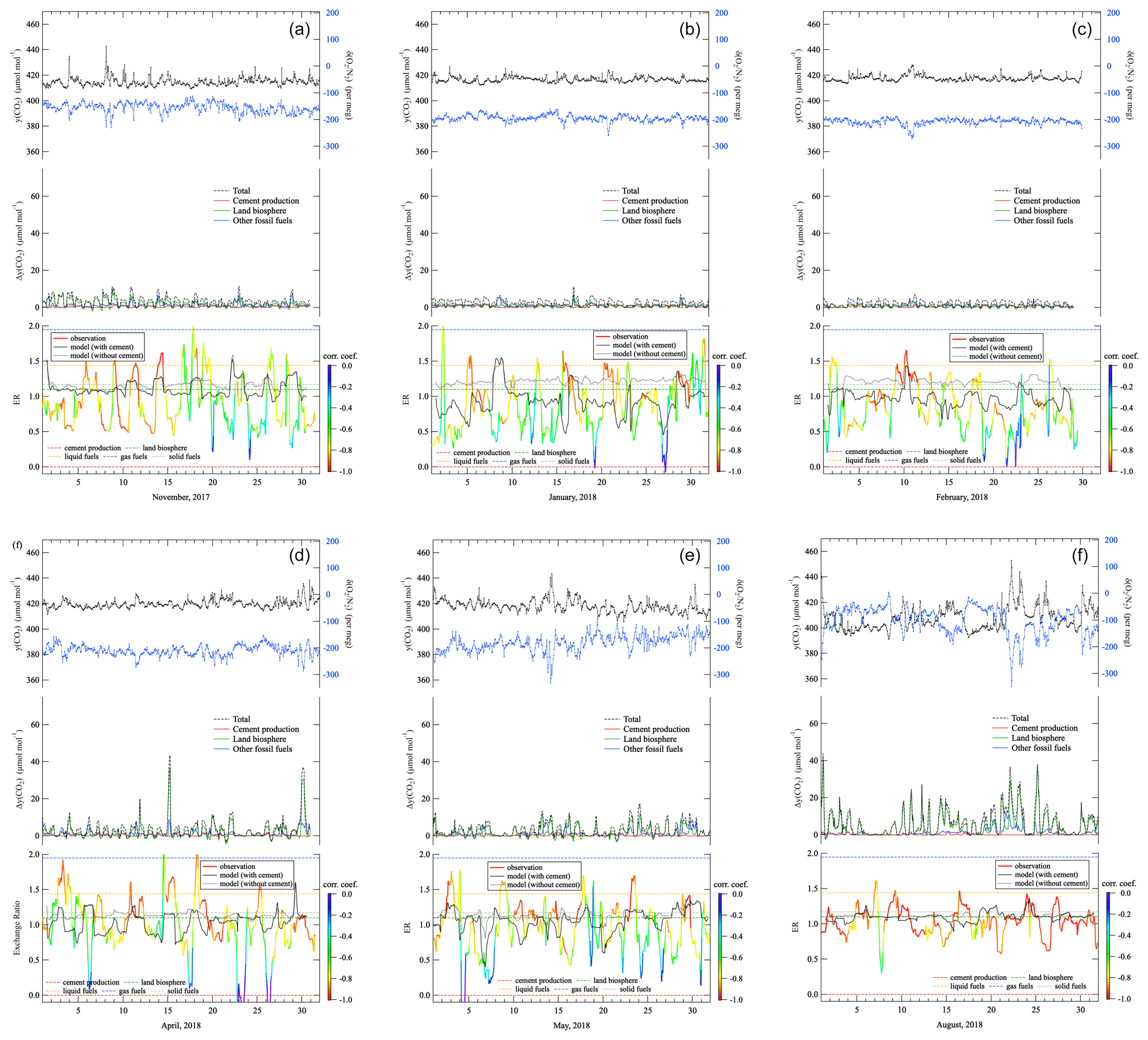
Figure B1(a) Same as in Fig. 5, but for November 2017. (b) As in (a), but for January 2018. (c) As in (a), but for February 2018. (d) As in (a), but for April 2018. (e) As in (a), but for May 2018. (f) As in (a), but for August 2018.
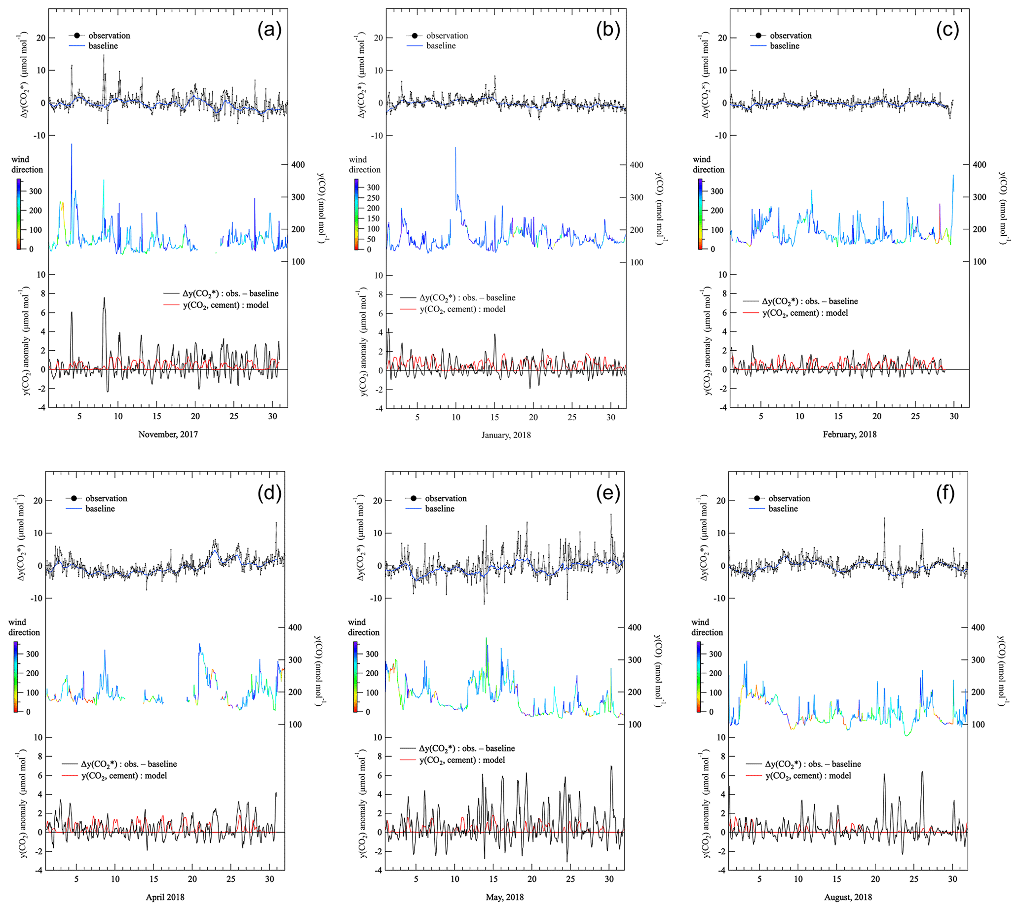
Figure B2(a) Same as in Fig. 6, but for November 2017. (b) As in (a), but for January 2018. (c) As in (a), but for February 2018. (d) As in (a), but for April 2018. (e) As in (a), but for May 2018. (f) As in (a), but for August 2018.
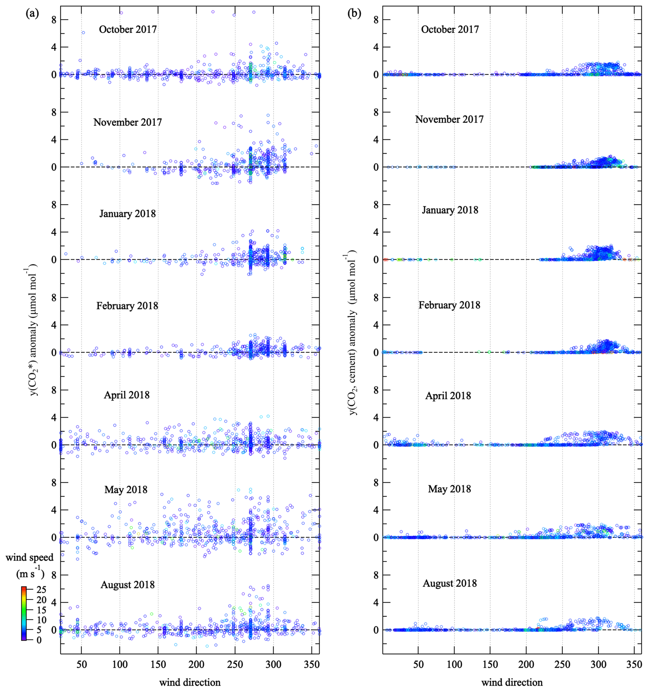
Figure B3(a) Relationships between anomaly shown in Figs. 6 and B2 and wind direction at RYO. (b) Same as in (a) but for y(CO2,cement). It is noted that the anomaly is 5 h average similar to Figs. 6 and B2 but the y(CO2,cement) is hourly values.
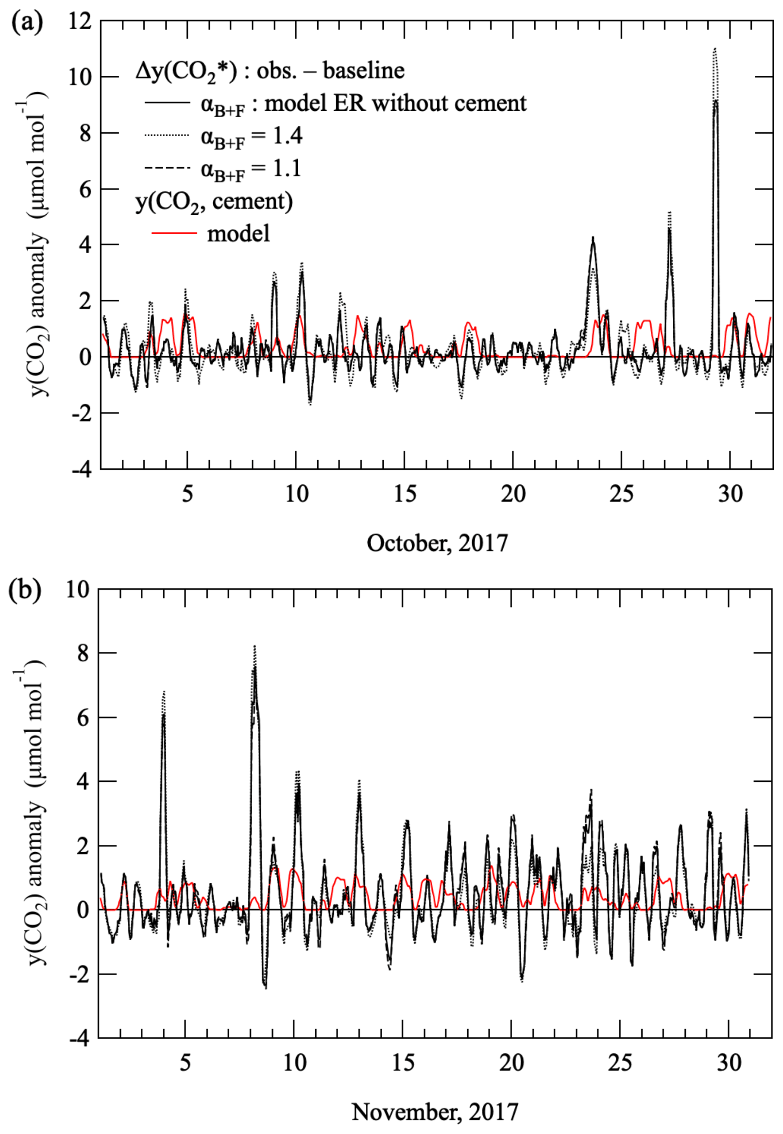
Figure B4(a) Same as in the bottom panels of Fig. 6, but for calculated by using model-simulated αB+F values (solid black line), and αB+F values of 1.4 (dotted black line) and 1.1 (dashed black line). (b) Same as in (a) but for the bottom panels of Fig. B2a.
The observational data of and the CO2 amount fraction are available through the World Data Centre for Greenhouse Gases (WDCGG) at https://gaw.kishou.go.jp (last access: 10 November 2023), and the respective DOIs are https://doi.org/10.50849/WDCGG_0006-2012-7001-01-01-9999 (Ishidoya, 2023a) and https://doi.org/10.50849/WDCGG_0006-2012-1001-01-01-9999 (Ishidoya, 2023b).
The supplement related to this article is available online at: https://doi.org/10.5194/acp-24-1059-2024-supplement.
SI designed the study and drafted the manuscript. Measurements of O2 and CO2 amount fractions were conducted by SI, KT, and KS. HK conducted the AIST-MM simulations. NA prepared the standard gas for the O2 measurements. KI and HM examined the results and provided feedback on the manuscript. All authors approved the final manuscript.
The contact author has declared that none of the authors has any competing interests.
Publisher’s note: Copernicus Publications remains neutral with regard to jurisdictional claims made in the text, published maps, institutional affiliations, or any other geographical representation in this paper. While Copernicus Publications makes every effort to include appropriate place names, the final responsibility lies with the authors.
We acknowledge the many staff members of the Japan Meteorological Agency. We also thank Shohei Murayama at the National Institute of Advanced Industrial Science and Technology (AIST), Ryo Fujita at the Meteorological Research Institute, and JANS Co. Ltd. for supporting the research.
This study was partly supported by JSPS KAKENHI (grant nos. 19H01975, 22H03739, and 22H05006) and the Global Environment Research Coordination System from the Ministry of the Environment, Japan (grant nos. METI1454 and METI1953).
This paper was edited by Jan Kaiser and reviewed by two anonymous referees.
Aoki, N., Ishidoya, S., Matsumoto, N., Watanabe, T., Shimosaka, T., and Murayama, S.: Preparation of primary standard mixtures for atmospheric oxygen measurements with less than 1 µmol mol−1 uncertainty for oxygen molar fractions, Atmos. Meas. Tech., 12, 2631–2646, https://doi.org/10.5194/amt-12-2631-2019, 2019.
Aoki, N., Ishidoya, S., Tohjima, Y., Morimoto, S., Keeling, R. F., Cox, A., Takebayashi, S., and Murayama, S.: Intercomparison of O2 N2 ratio scales among AIST, NIES, TU, and SIO based on a round-robin exercise using gravimetric standard mixtures, Atmos. Meas. Tech., 14, 6181–6193, https://doi.org/10.5194/amt-14-6181-2021, 2021.
Blaine, T. W., Keeling, R. F., and Paplawsky, W. J.: An improved inlet for precisely measuring the atmospheric ratio, Atmos. Chem. Phys., 6, 1181–1184, https://doi.org/10.5194/acp-6-1181-2006, 2006.
Bonan, G. B.: A Land surface model (LSM version 1.0) for ecological, hydrological, and atmospheric studies: Technical description and user's guide, Climate and global dynamics division, National Center for Atmospheric Research, Boulder, Colorado, 150 pp., https://doi.org/10.5065/D6DF6P5X, 1996.
Cohen, E. R., Cvitas, T., Frey, J. G., Holmstrom, B., Kuchitsu, K., Marquardt, R., Mills, I., Pavese, F., Quack, M., Stohner, J., Strauss, H., Takami, M., and Thor, A. J.: IUPAC Green Book: 3rd edn., RSC Publishing, ISBN 0854044337, ISBN 9780854044337, 2007.
Faassen, K. A. P., Nguyen, L. N. T., Broekema, E. R., Kers, B. A. M., Mammarella, I., Vesala, T., Pickers, P. A., Manning, A. C., Vilà-Guerau de Arellano, J., Meijer, H. A. J., Peters, W., and Luijkx, I. T.: Diurnal variability of atmospheric O2, CO2, and their exchange ratio above a boreal forest in southern Finland, Atmos. Chem. Phys., 23, 851–876, https://doi.org/10.5194/acp-23-851-2023, 2023.
Friedlingstein, P., O'Sullivan, M., Jones, M. W., Andrew, R. M., Gregor, L., Hauck, J., Le Quéré, C., Luijkx, I. T., Olsen, A., Peters, G. P., Peters, W., Pongratz, J., Schwingshackl, C., Sitch, S., Canadell, J. G., Ciais, P., Jackson, R. B., Alin, S. R., Alkama, R., Arneth, A., Arora, V. K., Bates, N. R., Becker, M., Bellouin, N., Bittig, H. C., Bopp, L., Chevallier, F., Chini, L. P., Cronin, M., Evans, W., Falk, S., Feely, R. A., Gasser, T., Gehlen, M., Gkritzalis, T., Gloege, L., Grassi, G., Gruber, N., Gürses, Ö., Harris, I., Hefner, M., Houghton, R. A., Hurtt, G. C., Iida, Y., Ilyina, T., Jain, A. K., Jersild, A., Kadono, K., Kato, E., Kennedy, D., Klein Goldewijk, K., Knauer, J., Korsbakken, J. I., Landschützer, P., Lefèvre, N., Lindsay, K., Liu, J., Liu, Z., Marland, G., Mayot, N., McGrath, M. J., Metzl, N., Monacci, N. M., Munro, D. R., Nakaoka, S.-I., Niwa, Y., O'Brien, K., Ono, T., Palmer, P. I., Pan, N., Pierrot, D., Pocock, K., Poulter, B., Resplandy, L., Robertson, E., Rödenbeck, C., Rodriguez, C., Rosan, T. M., Schwinger, J., Séférian, R., Shutler, J. D., Skjelvan, I., Steinhoff, T., Sun, Q., Sutton, A. J., Sweeney, C., Takao, S., Tanhua, T., Tans, P. P., Tian, X., Tian, H., Tilbrook, B., Tsujino, H., Tubiello, F., van der Werf, G. R., Walker, A. P., Wanninkhof, R., Whitehead, C., Willstrand Wranne, A., Wright, R., Yuan, W., Yue, C., Yue, X., Zaehle, S., Zeng, J., and Zheng, B.: Global Carbon Budget 2022, Earth Syst. Sci. Data, 14, 4811–4900, https://doi.org/10.5194/essd-14-4811-2022, 2022.
Fukui, T., Kokuryo, K., Baba, T., and Kannari, A.: Updating EAGrid2000-Japan emissions inventory based on the recent emission trends, J. Jpn. Soc. Atmos. Environ., 49, 117–125, 2014 (in Japanese).
Goto, D., Morimoto, S., Ishidoya, S., Ogi, A., Aoki, S., and Nakazawa, T.: Development of a high precision continuous measurement system for the atmospheric O2 N2 ratio and its application at Aobayama, Sendai, Japan, J. Meteorol. Soc. Jpn., 91, 179–192, 2013.
Goto, D., Morimoto, S., Aoki, S., Patra, P. K., and Nakazawa, T.: Seasonal and short-term variations in atmospheric potential oxygen at Ny-Ålesund, Svalbard, Tellus, 69B, 1311767, https://doi.org/10.1080/16000889.2017.1311767, 2017.
Hanna, S. R. and Chang, J. C.: Acceptance criteria for urban dispersion model evaluation, Meteorol. Atmos. Phys., 116, 133–146, 2012.
Ishidoya, S.: O2 N2 ratio_RYO_surface-insitu_AIST_data1, Atmospheric O2 N2 ratio at Ryori by National Institute of Advanced Industrial Science and Technology, ver. 2023-11-08-0331, World Data Centre for Greenhouse Gases (WDCGG) [data set], https://doi.org/10.50849/WDCGG_0006-2012-7001-01-01-9999, 2023a.
Ishidoya, S.: CO2_RYO_surface-insitu_AIST_data1, Atmospheric CO2 at Ryori by National Institute of Advanced Industrial Science and Technology, ver. 2023-11-08-0331, World Data Centre for Greenhouse Gases (WDCGG) [data set], https://doi.org/10.50849/WDCGG_0006-2012-1001-01-01-9999, 2023b.
Ishidoya, S. and Murayama, S.: Development of high precision continuous measuring system of the atmospheric O2 N2 and Ar N2 ratios and its application to the observation in Tsukuba, Japan, Tellus B, 66, 22574, https://doi.org/10.3402/tellusb.v66.22574, 2014.
Ishidoya, S., Murayama, S., Takamura, C., Kondo, H., Saigusa, N., Goto, D., Morimoto, S., Aoki, N., Aoki, S., and Nakazawa, T.: O2 : CO2 exchange ratios observed in a cool temperate deciduous forest ecosystem of central Japan, Tellus B, 65, 21120, https://doi.org/10.3402/tellusb.v65i0.21120, 2013.
Ishidoya, S., Tsuboi, K., Murayama, S., Matsueda, H., Aoki, N., Shimosaka, T., Kondo, H., and Saito, K.: Development of a continuous measurement system for atmospheric O2 N2 ratio using a paramagnetic analyzer and its application in Minamitorishima Island, Japan, SOLA, 13, 230–234, 2017.
Ishidoya, S., Sugawara, H., Terao, Y., Kaneyasu, N., Aoki, N., Tsuboi, K., and Kondo, H.: O2 : CO2 exchange ratio for net turbulent flux observed in an urban area of Tokyo, Japan, and its application to an evaluation of anthropogenic CO2 emissions, Atmos. Chem. Phys., 20, 5293–5308, https://doi.org/10.5194/acp-20-5293-2020, 2020.
Ishidoya, S., Tsuboi, K., Niwa, Y., Matsueda, H., Murayama, S., Ishijima, K., and Saito, K.: Spatiotemporal variations of the , CO2 and δ(APO) in the troposphere over the western North Pacific, Atmos. Chem. Phys., 22, 6953–6970, https://doi.org/10.5194/acp-22-6953-2022, 2022.
Japan Cement Association: Handbook of Cement, ISBN 978-88175-177-0 C600, 2020.
Kannari, A., Tonooka, Y., Baba, T., and Murano, K.: Development of multiple-species 1 km × 1 km resolution hourly basis emissions inventory for Japan, Atmos. Environ., 41, 3428–3439, 2007.
Development of an interferometric oxygen analyzer for precise measurement of the atmospheric O2 mole fraction, PhD thesis, Harvard University, USA, 1988.
Keeling, R. and Manning, A.: Studies of Recent Changes in Atmospheric O2 Content, in: Treatise on Geochemistry, 2nd edn., Elsevier Inc., 5, 385–404, https://doi.org/10.1016/B978-0-08-095975-7.00420-4, 2014.
Keeling, R. F. and Shertz, S. R.: Seasonal and interannual variations in atmospheric oxygen and implications for the global carbon cycle, Nature, 358, 723–727, 1992.
Keeling, R. F., Bender, M. L., and Tans, P. P.: What atmospheric oxygen measurements can tell us about the global carbon cycle, Global Biogeochem. Cy., 7, 37–67, 1993.
Keeling, R. F., Manning, A. C., and Dubey, M. K.: The atmospheric signature of carbon capture and storage, Philos. T. Roy. Soc. A, 369, 2113–2132, https://doi.org/10.1098/rsta.2011.0016, 2011.
Kondo, H., Saigusa, N., Murayama, S., Yamamoto, S., and Kannari, A.: A numerical simulation of the daily variation of CO2 in the central part of Japan – summer case, J. Meteor. Soc. Japan. Ser. II, 79, 11–21, 2001.
Liu, X., Huang, J., Wang, L., Lian, X., Li, C., Ding, L., Wei, Y., Chen, S., Wang, Y., Li, S., and Shi, J.: “Urban Respiration” Revealed by Atmospheric O2 Measurements in an Industrial Metropolis, Environ. Sci. Technol., 57, 2286–2296, https://doi.org/10.1021/acs.est.2c07583, 2023.
Minejima, C., Kubo, M., Tohjima, Y., Yamagishi, H., Koyama, Y., Maksyutov, S., Kita, K., and Mukai, H.: Analysis of ratios for the pollution events observed at Hateruma Island, Japan, Atmos. Chem. Phys., 12, 2713–2723, https://doi.org/10.5194/acp-12-2713-2012, 2012.
Nakazawa, T., Sugawara, S., Inoue, G., Machida, T., Makshutov, S. and Mukai, H.: Aircraft measurements of the concentrations of CO2, CH4, N2O and CO and the carbon and oxygen isotopic ratios of CO2 in the troposphere over Russia, J. Geophys. Res., 102, 3843–3859, 1997.
Nara, H., Tanimoto, H., Nojiri, Y., Mukai, H., Zeng, J., Tohjima, Y., and Machida, T.: CO emissions from biomass burning in South-east Asia in the 2006 El Niño year: shipboard and AIRS satellite observations, Environ. Chem., 8, 213–223, https://doi.org/10.1071/EN10113, 2011.
Niwa, Y., Tsuboi, K., Matsueda, H., Sawa, Y., Machida, T., Nakamura, M., Kawasato, T., Saito, K., Takatsuji, S., Tsuji, K., Nishi, H., Dehara, K., Baba, Y., Kuboike, D., Iwatsubo, S., Ohmori, H., and Hanamiya, Y.: Seasonal Variations of CO2, CH4, N2O and CO in the Mid-troposphere over the Western North Pacific Observed using a C-130H Cargo Aircraft, J. Meteorol. Soc. Jpn., 92, 55–70, https://doi.org/10.2151/jmsj.2014-104, 2014.
Pak, N. M., Rempillo, O., Norman, A.-L., and Layzell, D. B.: Early atmospheric detection of carbon dioxide from carbon capture and storage sites, J. Air Waste Manag. Assoc., 66, 739–747, https://doi.org/10.1080/10962247.2016.1176084, 2016.
Pickers, P. A., Manning, A. C., Le Quéré, C., Forster, G. L., Luijkx, I. T., Gerbig, C., Fleming, L. S., and Sturges, W. T.: Novel quantification of regional fossil fuel CO2 reductions during COVID-19 lockdowns using atmospheric oxygen measurements, Science Advances, 8, eabl9250, https://doi.org/10.1126/sciadv.abl9250, 2022.
Resplandy, L., Keeling, R.F., Eddebbar, Y., Brooks, M., Wang, R., Bopp, L., Long, M. C., Dunne, J. P., Koeve, W., and Oschlies, A.: Quantification of ocean heat uptake from changes in atmospheric O2 and CO2 composition, Scientific Reports, 9, 20244, https://doi.org/10.1038/s41598-019-56490-z, 2019.
Severinghaus, J.: Studies of the terrestrial O2 and carbon cycles in sand dune gases and in biosphere 2, PhD thesis, Columbia University, New York, 1995.
Stephens, B. B., Keeling, R. F., Heimann, M., Six, K. D., Murnane, R., and Caldeira, K.: Testing global ocean carbon cycle models using measurements of atmospheric O2 and CO2 concentration, Global Biogeochem. Cy., 12, 213–230, 1998.
Sugawara, H., Ishidoya, S., Terao, Y., Takane, Y., Kikegawa, Y., and Nakajima, K.: Anthropogenic CO2 emissions changes in an urban area of Tokyo, Japan, due to the COVID-19 pandemic: A case study during the state of emergency in April–May 2020, Geophys. Res. Lett., 48, e2021GL092600, https://doi.org/10.1029/2021GL092600, 2021.
Tohjima, Y., Machida, T., Watai, T., Akama, I., Amari, T., and Moriwaki, Y.: Preparation of gravimetric standards for measurements of atmospheric oxygen and reevaluation of atmospheric oxygen concentration, J. Geophys. Res., 110, D1130, https://doi.org/10.1029/2004JD005595, 2005.
Tohjima, Y., Kubo, M., Minejima, C., Mukai, H., Tanimoto, H., Ganshin, A., Maksyutov, S., Katsumata, K., Machida, T., and Kita, K.: Temporal changes in the emissions of CH4 and CO from China estimated from CH4 CO2 and CO CO2 correlations observed at Hateruma Island, Atmos. Chem. Phys., 14, 1663–1677, https://doi.org/10.5194/acp-14-1663-2014, 2014.
Tsuboi, K., Matsueda, H., Sawa, Y., Niwa, Y., Takahashi, M., Takatsuji, S., Kawasaki, T., Shimosaka, T., Watanabe, T., and Kato, K.: Scale and stability of methane standard gas in JMA and comparison with MRI standard gas, Pap. Meteorol. Geophys., 66, 15–24, 2016.
van Leeuwen, C. and Meijer, H. A. J.: Detection of CO2 leaks from carbon capture and storage sites with combined atmospheric CO2 and O2 measurements, Int. J. Greenh. Gas Control, 41, 194–209, 2015.
Wada, A., Matsueda, H., Sawa, Y., Tsuboi, K., and Okubo, S.: Seasonal variation of enhancement ratios of trace gases observed over 10 years in the western North Pacific, Atmos. Environ., 45, 2129–2137, 2011.
Yamagishi, H., Tohjima, Y., Mukai, H., and Sasaoka, K.: Detection of regional scale sea-to-air oxygen emission related to spring bloom near Japan by using in-situ measurements of the atmospheric oxygen/nitrogen ratio, Atmos. Chem. Phys., 8, 3325–3335, https://doi.org/10.5194/acp-8-3325-2008, 2008.
- Abstract
- Introduction
- Methods
- Results and discussion
- Conclusions
- Appendix A: Additional figures to evaluate the effect of entrainment of air mass on the observed ER
- Appendix B: Additional figures to evaluate the effect of cement production on the observed and simulated CO2 amount fractions
- Data availability
- Author contributions
- Competing interests
- Disclaimer
- Acknowledgements
- Financial support
- Review statement
- References
- Supplement