Automated detection of regions with persistently enhanced methane concentrations using Sentinel-5 Precursor satellite data

Methane (CH₄) is an important anthropogenic greenhouse gas, and its rising concentration in the atmosphere contributes significantly to global warming. A comparatively small number of highly emitting persistent methane sources are responsible for a large share of global methane emissions. The identification and quantification of these sources, which often show large uncertainties regarding their emissions or locations, are important to support mitigating climate change. Daily global column-averaged dry air mole fractions of atmospheric methane (XCH₄) are retrieved from radiance measurements of the TROPOspheric Monitoring Instrument (TROPOMI) on board on the Sentinel-5 Precursor (S5P) satellite with a moderately high spatial resolution, enabling the detection and quantification of localized methane sources. We developed a fully automated algorithm to detect regions with persistent methane enhancement and to quantify their emissions using a monthly TROPOMI XCH₄ dataset from the years 2018–2021. We detect 217 potential persistent source regions (PPSRs), which account for approximately 20 % of the total bottom-up emissions. By comparing the PPSRs in a spatial analysis with anthropogenic and natural emission databases, we conclude that 7.8 % of the detected source regions are dominated by coal, 7.8 % by oil and gas, 30.4 % by other anthropogenic sources like landfills or agriculture, 7.3 % by wetlands, and 46.5 % by unknown sources. Many of the identified PPSRs are in well-known source regions, like the Permian Basin in the USA, which is a large production area for oil and gas; the Bowen Basin coal mining area in Australia; or the Pantanal Wetlands in Brazil. We perform a detailed analysis of the PPSRs with the 10 highest emission estimates, including the Sudd Wetland in South Sudan, an oil- and gas-dominated area on the west coast in Turkmenistan, and one of the largest coal production areas in the world, the Kuznetsk Basin in Russia. The calculated emission estimates of these source regions are in agreement within the uncertainties in results from other studies but are in most of the cases higher than the emissions reported by emission databases. We demonstrate that our algorithm is able to automatically detect and quantify persistent localized methane sources of different source type and shape, including larger-scale enhancements such as wetlands or extensive oil- and gas-production basins.

1 Introduction

Methane (CH₄) is the second-most-important anthropogenic greenhouse gas after carbon dioxide (CO₂), and its increasing concentration in the atmosphere, which has accelerated in recent years, contributes significantly to global warming (Lan et al., 2021). Due to its shorter lifetime and higher global warming potential compared to CO₂, the reduction in methane emissions can contribute to mitigation of global warming (Shoemaker et al., 2013).

Almost half of the global methane emissions originate from anthropogenic sources, which are dominated by fossil fuel exploitation, livestock, rice cultivation and landfills, whereas the natural emissions mainly originate from wetlands (Saunois et al., 2020). To efficiently reduce methane emissions, a comprehensive understanding of the natural and anthropogenic methane sources and sinks is required. However, global methane emissions are characterized by large uncertainties, as can be seen in bottom-up inventories, which have uncertainties of 20 %–35 % for anthropogenic emissions regarding agriculture, fossil fuel and waste and 50 % for wetland emissions (Saunois et al., 2020). These uncertainties are strongly related to emissions from individual sources, which are highly uncertain or even partly unknown, especially on a regional scale (Saunois et al., 2020). Consequently, explanation of the observed atmospheric methane trends remains challenging. For example, the abundance of atmospheric methane grew until 1998, remained at a constant plateau until 2006 and then started to grow again. The reasons for this unique behavior are still highly debated (Nisbet et al., 2016; Turner et al., 2019). Also, the accelerated increase in recent years is still the subject of ongoing research, with several studies concluding that the rise was dominated by an increase in wetland emissions (Lan et al., 2021; Peng et al., 2022; Zhao et al., 2020).

In particular, strongly emitting methane sources have a substantial impact on global methane emissions. These include small-scale point sources, so-called super-emitters, such as individual coal mines, natural gas compressor stations or landfills (He et al., 2024; Lauvaux et al., 2022; Maasakkers et al., 2022; Schuit et al., 2023; Varon et al., 2019). A comparatively small number of those super-emitters are responsible for a large proportion of methane emissions associated with oil and gas exploitation, coal mining and waste (Frankenberg et al., 2016; Jacob et al., 2016; Lauvaux et al., 2022; Zavala-Araiza et al., 2015). In addition to the super-emitters, larger-scale but localized source regions also contribute a large share to global methane emissions. These include large oil and gas fields, where smaller sources can emit a huge amount of methane in aggregate, but also regions with high agricultural productivity (rice cultivation, livestock), as well as wetland areas (Buchwitz et al., 2017; Chen et al., 2024; Naus et al., 2023; Pandey et al., 2021; Schneising et al., 2020). The detection and quantification of these small-scale super-emitters and larger-scale source areas is essential to assess the contribution of these sources to the global methane emissions and to identify their inherent potential for reducing the global emissions.

Ground-based and aircraft measurements have been used to quantify localized methane sources but are limited in time and/or space, making (frequent) observations of remote source regions difficult (Borchardt et al., 2021; Frankenberg et al., 2016; Krautwurst et al., 2021). Satellite measurements, such as from the SCanning Imaging Absorption spectroMeter for Atmospheric CHartographY (SCIAMACHY; Burrows et al., 1995; Bovensmann et al., 1999) or the Greenhouse gases Observing SATellite (GOSAT; Kuze et al., 2009, 2016), offer the possibility of globally detecting and quantifying localized emission sources through temporally frequent global measurements of atmospheric methane (Buchwitz et al., 2017; Jacob et al., 2016, 2022; Sherwin et al., 2024; Thorpe et al., 2023). One important breakthrough in satellite remote sensing of methane in recent years was achieved by the successful launch of the Sentinel-5 Precursor (S5P) satellite in October 2017. Onboard S5P is the TROPOspheric Monitoring Instrument (TROPOMI), which is a nadir-viewing spectrometer (Veefkind et al., 2012). It provides observations in the shortwave infrared (SWIR) spectral range with a spatial resolution of 5.5×7 km², from which column-averaged dry air mole fractions of atmospheric methane (XCH₄) can be retrieved. Due to the high sensitivity to near-surface concentration changes and the combination of daily global coverage with moderately high spatial resolution, TROPOMI data have already been used to quantify emissions on global and regional scales, including a wide variety of methane sources, such as transient gas leaks, oil and gas fields, coal mining, and urban areas, as well as from wetland regions (Liu et al., 2021; Naus et al., 2023; Qu et al., 2021; Pandey et al., 2019; Plant et al., 2022; Schneising et al., 2020; Varon et al., 2023; Veefkind et al., 2023). In addition to emission quantification, various studies have shown that TROPOMI can be used to identify point sources on a global scale via plume detection (Lauvaux et al., 2022; Schuit et al., 2023) or via combination with model forecasts (Barré et al., 2021). For example, Barré et al. (2021) created a monitoring methodology to detect CH₄ concentration anomalies by comparing TROPOMI data with high-resolution CH₄ forecasts from the Copernicus Atmosphere Monitoring Service (CAMS). This method can be used to detect missing, underreported and overreported CH₄ anomalies in the CAMS data worldwide. Lauvaux et al. (2022) detected methane super-emitters associated with oil and gas production and exploitation for 2019–2020 by analyzing daily TROPOMI data using a plume detection algorithm based on the calculation of local XCH₄ enhancements and plume segmentation. The super-emitters were mostly detected over the largest oil and gas basins in Russia, Turkmenistan, the USA, Algeria and the Middle East and amount to 8 %–12 % of the global oil and gas emissions. Schuit et al. (2023) used TROPOMI data to identify anthropogenic super-emitters including emissions from the coal, oil, gas and landfill sectors for 2021 using a machine-learning approach based on a convolutional neural network to detect plume-like structures and a support vector classifier to distinguish between real plumes and retrieval artifacts. Methane plumes originating from super-emitters worldwide were identified, mostly from persistent emission clusters but also from transient sources.

The focus of the studies from Barré et al. (2021), Lauvaux et al. (2022) and Schuit et al. (2023) is on the detection of strongly emitting anthropogenic point sources, for example via plume detection. But besides super-emitters, numerous larger-scale strong source regions of different source types exist, in which the emissions do not have a plume-like structure as the signals of individual sources within the regions can interfere. This can be the case, for example, in large oil and gas fields or wetlands (Lauvaux et al., 2022; Naus et al., 2023; Pandey et al., 2021). To include such source regions in a detection procedure was an important motivation for this study. Therefore, we developed an automated algorithm to detect and quantify source regions of various sizes, regardless of their source type, including small-scale super-emitters such as coal mine ventilation shafts but also larger-scale source areas such as wetland areas and large oil and gas fields. Since source regions with strong and persistent methane enhancements contribute significantly to global methane emissions, we have focused on such source regions in this study. TROPOMI has been providing a vast amount of daily methane data since its launch in 2017. To allow for the detection of methane source regions in this large dataset on a global scale, we fully automated our detection algorithm. The data-driven detection algorithm is based on several steps, including high-pass filtering of the TROPOMI data and masking of regions with persistent methane enhancements by applying different threshold criteria. In addition to detection, our algorithm includes a characterization of the source regions, in which the dominant source type is assigned, and an emission estimate for each source region is determined.

This study is structured as follows. In Sect. 2, we first present the data that we used for the detection and characterization of the source regions. In Sect. 3, we describe the algorithm. In Sect. 4, we present our results, including a global overview of the detected source regions and a detailed analysis of the source regions with the 10 highest emission estimates by comparing our results with emission databases and results from recent studies. At the end, in Sect. 5, we present our conclusions.

2 Data

2.1 TROPOMI/WFMD XCH₄ data product

The Sentinel-5 Precursor (S5P) satellite with the TROPOspheric Monitoring Instrument (TROPOMI) on board was launched in October 2017 in a near-polar, sun-synchronous orbit with an equatorial crossing of the ascending node at 13:30 local solar time. TROPOMI is a nadir-viewing spectrometer and operates in a push-broom configuration with a swath width of 2600 km, enabling daily global coverage. It measures solar radiation reflected at the Earth's surface in the ultraviolet (267–332 nm), ultraviolet-visible (305–499 nm), near-infrared (661–786 nm) and shortwave infrared (2300–2389 nm) spectral channels (Veefkind et al., 2012). The measurements of TROPOMI in the shortwave infrared (SWIR) spectral range enable the retrieval of column-averaged dry-air mole fractions of atmospheric methane (XCH₄), with a horizontal resolution of 5.5×7 km² (7×7 km² before August 2019). The radiation backscattered from the earth's surface and measured at the top of the atmosphere has passed through the planetary boundary layer. Therefore, TROPOMI's measurements yield the gas absorption throughout the atmosphere and importantly close to the earth's surface (Schneising et al., 2019). Consequently, the retrieved XCH₄ can be used to detect methane enhancements originating from localized methane sources at the Earth's surface.

In this study, we use a multi-year (2018–2021) TROPOMI XCH₄ dataset retrieved with the Weighting Function Modified Differential Optical Absorption Spectroscopy (WFMD) retrieval algorithm (Buchwitz et al., 2006; Schneising et al., 2011, 2014), which has been adapted and optimized for use on TROPOMI data (Schneising et al., 2019). We use the latest version (v1.8) of the TROPOMI/WFMD product (Schneising et al., 2023) and average the data to monthly XCH₄ maps with a spatial resolution of 0.1°×0.1°. In addition to the XCH₄, the dataset also includes two variables that are needed for the detection and characterization of the source regions. These variables are (i) the retrieved surface albedo in the SWIR spectral range and (ii) for each monthly averaged XCH₄ grid cell, the number of days, N_days, with TROPOMI measurements from which the monthly mean was calculated. In the following, we refer to this dataset consisting of the 0.1°×0.1° monthly maps of XCH₄, SWIR albedo and N_days as the XCH₄ dataset.

2.2 Wind data

Wind data are required to calculate emissions. The European Centre for Medium-Range Weather Forecasts (ECMWF) reanalysis (ERA5) wind product (Hersbach et al., 2020) provides hourly wind data with a horizontal resolution of 0.25°×0.25° on model levels. From this dataset, we computed boundary-layer-averaged wind speed at the overpass time of TROPOMI for each TROPOMI sounding. The resulting winds are then gridded in the same way as the XCH₄ dataset to monthly maps with a spatial resolution of 0.1°×0.1°. In addition to the monthly averaged wind speeds, we computed the standard deviation of the wind speed within the months for each grid cell.

2.3 Surface elevation and roughness

The Global Multi-resolution Terrain Elevation Data 2010 (GMTED 2010) is a dataset containing global surface elevation data available at three different resolutions (approximately 250, 500 and 1000 m) from various data sources (Danielson and Gesch, 2011). We use the GMTED 2010 to assign the mean surface elevation and the standard deviation of the surface elevation (surface roughness) within the grid cells to the 0.1°×0.1° grid cells of the XCH₄ dataset.

2.4 Emission databases

We use the following emission databases to determine the dominant source types of the detected potential source regions by comparing the emissions of the databases.

2.4.1 EDGAR

The Emissions Database for Global Atmospheric Research (EDGAR) v6.0 (Ferrario et al., 2021) is a bottom-up inventory providing detailed information about global anthropogenic emissions of various air pollutants and greenhouse gases. The yearly emission data have a spatial resolution of 0.1°×0.1° and are available from 1970 to 2018. The emissions of a specific gas are calculated using international activity data and emission factors using the IPCC (Eggleston et al., 2006) methodology. Activity data describe the activities producing emissions, such as the amount of fossil fuel that is exploited or the number of animals on a farm. Emission factors are coefficients that relate the emitted amount of a specific gas to a certain activity or process. The data required to calculate the emissions are collected from a variety of sources, including international organizations such as the International Energy Agency (IEA), national emission inventories and industry reports. EDGAR is well-suited to determine the anthropogenic source types of the detected potential since this inventory provides sector-specific emissions, which enables the differentiation between individual source types within the source regions. For methane, EDGAR v6.0 provides sector-specific anthropogenic emissions from, for example, enteric fermentation; landfills; rice cultivation; and fossil fuel exploitation, which is further separated into coal, oil, and gas emissions. We use the EDGAR v6.0 methane data for 2018.

2.4.2 GFEI

The Global Fuel Emission Inventory (GFEI) v2.0 (Scarpelli et al., 2022) is a methane emission database providing global anthropogenic emissions for the fossil fuel sectors: coal, oil and gas. The emission data are gridded to yearly maps (2010–2019) with a resolution of 0.1°×0.1°. GFEI v2.0 uses fossil-fuel-related emission data reported by countries to the United Nations Framework Convention on Climate Change (UNFCCC); separated into the sectors of coal, oil, and gas; and assigned to the appropriate infrastructure locations like coal mines or oil and gas wells. The infrastructure data are taken from several databases. For countries that do not report their emissions to the UNFCCC, the emissions are calculated using the IPCC (Eggleston et al., 2006) methods and activity data from the US Energy Information Administration (EIA). Due to the different methods and data used for emission quantification in EDGAR v6.0 and GFEI v2.0, both databases show differences in their fossil fuel emissions, especially on a regional scale. Therefore, GFEI v2.0 can be used as a useful supplementary database to assign the appropriate fossil fuel source type to the detected source regions. We use GFEI v2.0 data for 2019.

2.4.3 WetCHARTs

WetCHARTs v1.3.1 is a global wetland methane emission ensemble that provides monthly emissions with a resolution of 0.5°×0.5° for the time period of 2001–2019 (Bloom et al., 2021). The ensemble is based on different wetland extent scenarios, multiple terrestrial biosphere models and various temperature dependence parameterizations, resulting in 18 different model configurations. We use WetCHARTs to also include wetlands as a potential dominant source type of a source region. To compare the wetland emissions from WetCHARTs with the other emission databases, we create a yearly averaged wetland emission map for 2019, with a resolution of 0.1°×0.1°, by averaging the emissions of all configurations and months.

3 Methods

We have developed a data-driven persistent hotspot detection (PHD) algorithm to automatically detect regions with persistent XCH₄ enhancements, to estimate their emissions and to assign a source type to these regions. The individual steps of the detection algorithm are shown in Fig. 1. As input to the PHD algorithm, we use the XCH₄ dataset (Sect. 2.1), the wind dataset (Sect. 2.2), the surface elevation data according to GMTED 2010 (Sect. 2.3), and the two anthropogenic emission inventories EDGAR v6.0 and GFEI v2.0, as well as the wetland emission dataset WetCHARTs v1.3.1 (Sect. 2.4). First, we process the XCH₄ dataset (Sect. 3.1). This step includes filtering out grid cells that contain XCH₄ only in a few days within a month. For the detection of localized enhancements, we filter out large-scale XCH₄ variations by applying a high-pass filter with five different kernel sizes to each monthly XCH₄ map (Sect. 3.2), resulting in five datasets that contain the local anomalies, ΔXCH₄. In the next step, we analyze the ΔXCH₄ datasets to detect persistent source regions (Sect. 3.3). For this, we first identify individual grid cells with persistent enhancement and then merge them into potential source regions. Afterwards, we conservatively filter out detected source regions, which may be false positives due to challenging surface features. For each of the five ΔXCH₄ datasets, we obtain one global map of the detected potential source regions. In the next step, we combine all of the detected source regions into one map (Sect. 3.4) before we estimate their emissions (Sect. 3.5). In the final step, we determine the dominant source types of the source regions by applying a spatial analysis based on the comparison of the methane emission databases within the source regions. As a result of the PHD algorithm, we obtain a list with the characteristics of the detected source regions. The list includes the locations, the estimated emissions and the assigned dominant source types of the source regions. In the following, we describe the steps of the algorithm in more detail.

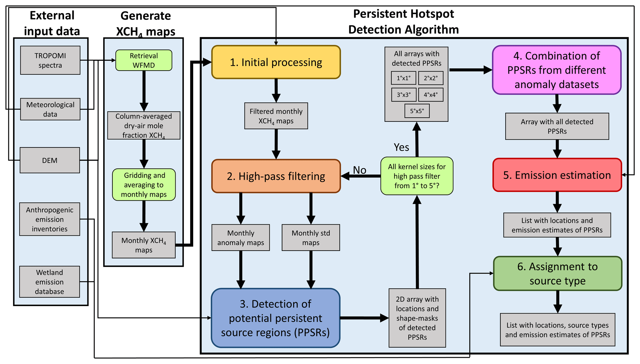
Figure 1 Flowchart of the persistent hotspot detection (PHD) algorithm version 1.0. The colored boxes symbolize the steps in which data are processed and analyzed. The gray boxes describe the input and/or output data of these steps. For a detailed description of the algorithm, see Sect. 3.1–3.6.

3.1 Initial processing

To optimize the XCH₄ dataset (Sect. 2.1) for the detection of persistent XCH₄ enhancements, we transform it into a new dataset, XCH₄*. For this, we apply filtering and a so-called elevation correction, which are described in the following. For the detection of persistent source regions, we only consider grid cells in which the monthly XCH₄ means were calculated from more than 3 d of TROPOMI measurements (N_days>3).

Changes in surface elevation and tropopause height lead to variations in the tropospheric fraction of the XCH₄ (Kort et al., 2014; Buchwitz et al., 2017). Because the mean mixing ratio of methane is higher in the troposphere than in the stratosphere, the XCH₄ over a valley is enhanced compared to its surrounding area, even if the valley is not a source region. To correct for these topography-related variations, we apply an elevation correction to the XCH₄ (Buchwitz et al., 2017). We normalize the XCH₄ to mean sea level by adding 8.5 ppb per kilometer above mean sea level to the XCH₄ of the grid cells. We calculated this value following the approach of Buchwitz et al. (2017). To determine the surface elevation of the grid cells, we use the surface elevation data described in Sect. 2.3.

We denote the filtered and elevation-corrected data XCH₄*. Figure 2 shows the global maps for 2018–2021 of XCH₄ and XCH₄*. The data gaps in Fig. 2b are due to the removal of grid cells that contain XCH₄ only in a few days. The effect of the elevation correction can be seen in Fig. 2b in the higher XCH₄ over areas with high surface elevation (e.g., the Himalaya) compared to the uncorrected dataset. In the following sections, we always refer to XCH₄* when we mention XCH₄.

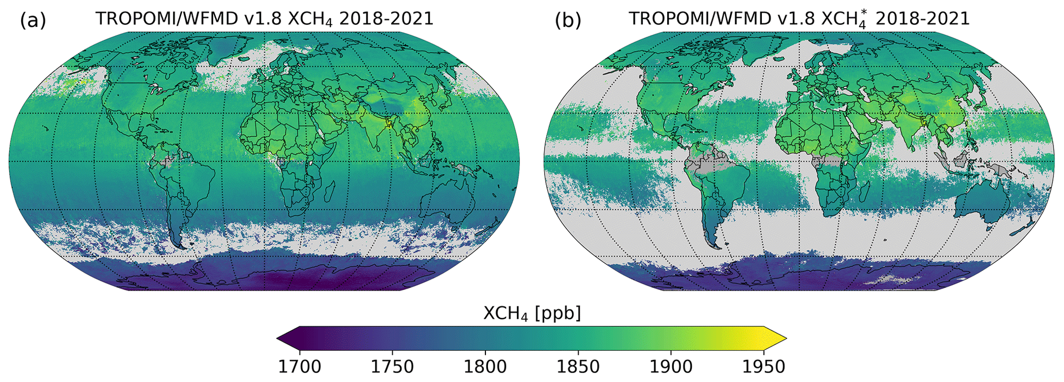
Figure 2 (a) Multi-year (2018–2021) XCH₄ and (b) the corresponding filtered and elevation-corrected XCH₄*.

3.2 High-pass filtering

The spatial distribution of global methane concentration shows large-scale methane variations, such as the interhemispheric gradient (Fig. 2a). To better detect localized XCH₄ enhancements, we minimize these large-scale variations by applying a high-pass filter with five different kernel sizes to each monthly XCH₄ map (see Sect. 3.1). For each kernel size, we obtain one dataset, which consists of monthly maps showing only the local XCH₄ variations. The high-pass filtering comprises three steps and is applied to each grid cell of a monthly XCH₄ map as follows. First, we define an area of size n°×n° around the grid cell considered, denoted the high-pass filter area (HPFA(n)), with $n\in \mathit{\{}\mathrm{1},\mathrm{2},\mathrm{3},\mathrm{4},\mathrm{5}\mathit{\}}$. Second, the HPFA(n) has to be filled with at least 25 % data. Otherwise, the grid cell is removed. Third, we calculate the so-called methane anomaly, ΔXCH₄, by calculating the difference in the XCH₄ of the grid cell with the corresponding median $\stackrel{\mathrm{̃}}{{\mathrm{XCH}}_{\mathrm{4}}}$ in the HPFA(n):

$$\begin{array}{}\text{(1)}& \mathrm{\Delta }{\mathrm{XCH}}_{\mathrm{4}}={\mathrm{XCH}}_{\mathrm{4}}-\stackrel{\mathrm{̃}}{{\mathrm{XCH}}_{\mathrm{4}}}{|}_{\mathrm{HPFA}}.\end{array}$$

The steps of the anomaly calculation are illustrated in Fig. 3a–c. In the next sections, we use the anomalies to identify potential source regions. For this, the HPFA(n) used has to be larger than the source region so that the HPFA(n) contains XCH₄ that is not enhanced. Otherwise, the anomalies only describe the variations within the source regions and not their enhancements. However, the HPFA(n) must not be too large as it could contain XCH₄ that is influenced by other nearby sources. Since the potential source regions to be detected have different spatial extents, ranging from small point sources to larger-scale areas, we choose five different HPFA(n) sizes from n=1° to n=5° to consider source regions with various sizes.

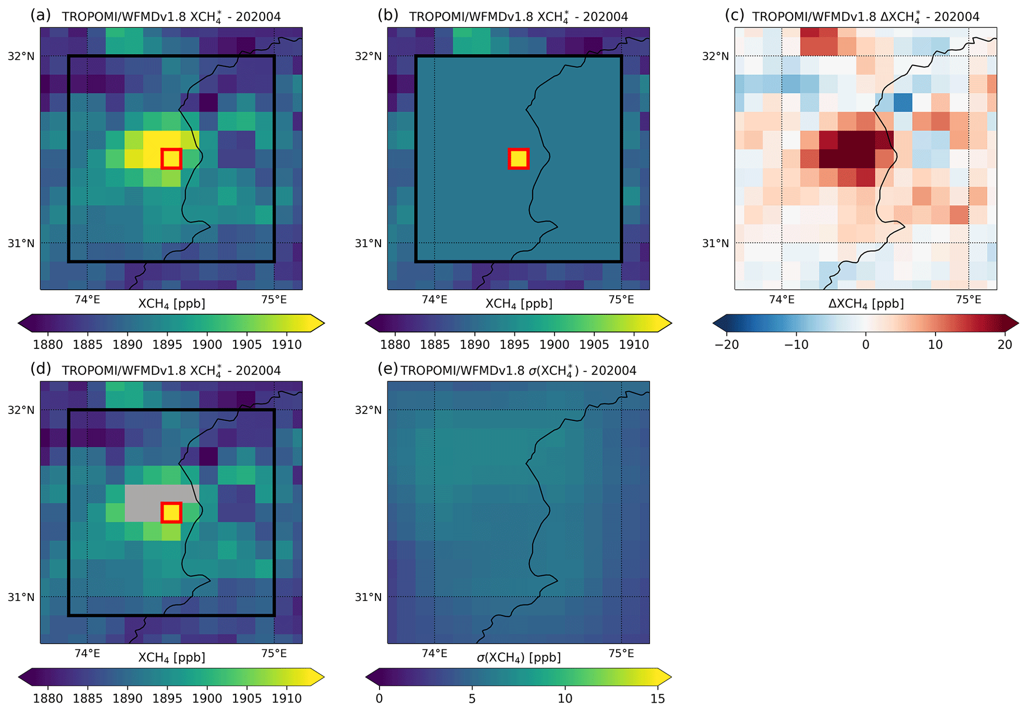
Figure 3 Illustration of the steps to calculate the methane anomaly and standard deviation maps described in Sect. 3.2. (a) XCH₄ for April 2020 for a region close to the border of Pakistan/India. The anomaly calculation process is illustrated for one grid cell shown in red. First, the HPFA(n) is defined, which is 1°×1° in this example. (b) The median of the XCH₄ values in the HPFA is calculated, with the XCH₄ of the grid cell considered excluded from the calculation. The anomaly of the grid cell considered is computed using Eq. 1. (c) ΔXCH₄ for April 2020 calculated using an HPFA of 1°×1°. The anomalies illustrate the XCH₄ enhancement in panel (a). (d) Illustration of the process to calculate the standard deviation of the XCH₄ values in the HPFA. First, the 95th percentile of the XCH₄ values within the HPFA is computed. All XCH₄ values above the 95th percentile are excluded from the standard deviation calculation to reduce the impact of local enhancements. (e) Standard deviation of the XCH₄ in the HPFA of 1°×1° for April 2020.

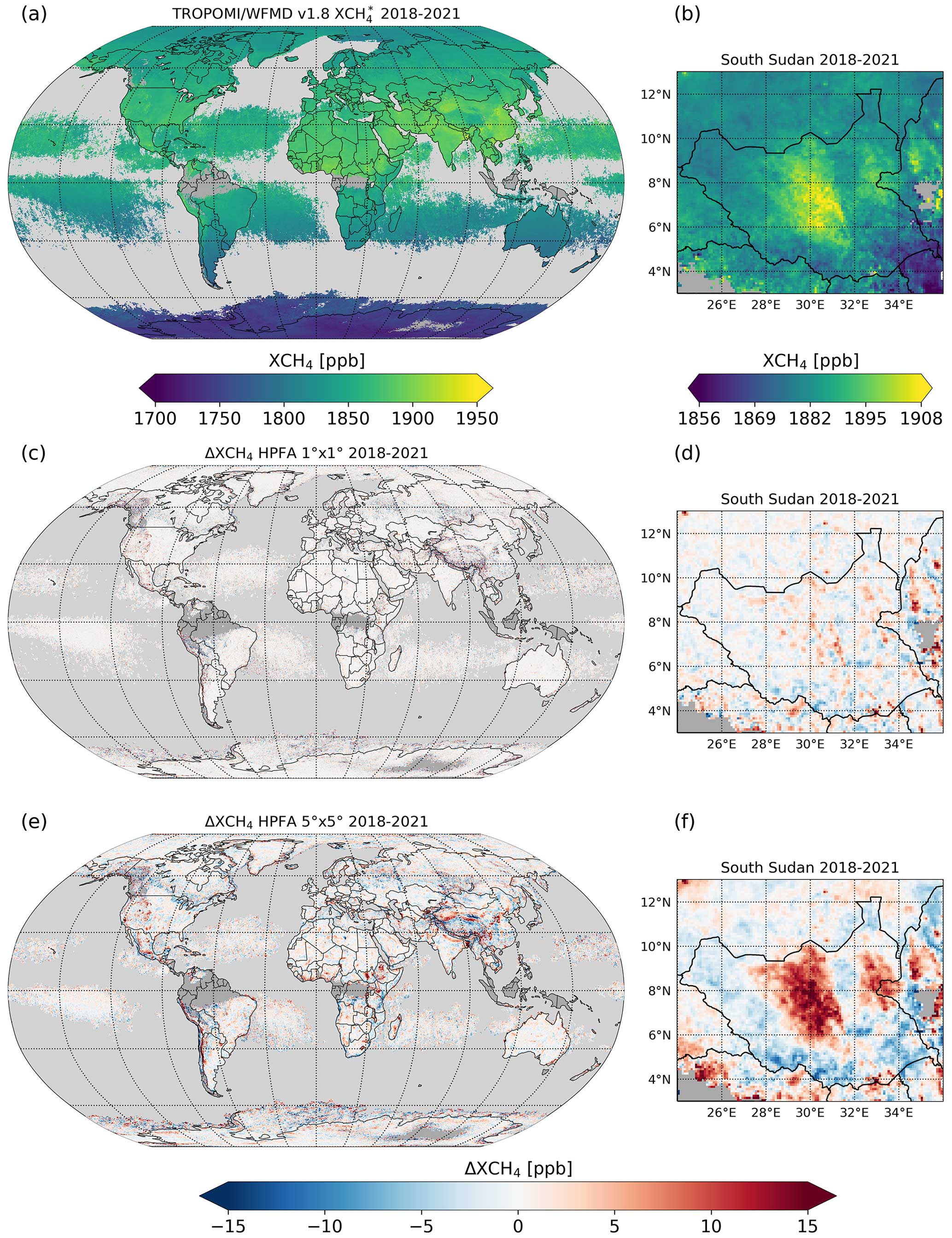
Figure 4 Comparison of global (a, c, e) and regional (b, d, f) multi-year (2018–2021) XCH₄ and ΔXCH₄ maps. (a) Same as Fig. 2b. (b) Corresponding zoom of South Sudan. (c) ΔXCH₄ calculated with an HPFA of 1°×1°. (d) Zoom of South Sudan for a 1°×1° ΔXCH₄ map. (e) As (c) but for an HPFA of 5°×5°. (f) Zoom of South Sudan for a 5°×5° ΔXCH₄ map.

Figure 4 shows two multi-year ΔXCH₄ maps on global and regional scales, calculated with HPFA sizes of 1° and 5° (panels c–f), and the corresponding XCH₄ map (a–b). On the left side, the global maps are shown. It can be seen that the large-scale variations have been minimized in the ΔXCH₄ maps. The ΔXCH₄ maps contain less data compared to the XCH₄ map because grid cells whose HPFA(n) does not contain the minimum amount of XCH₄ data are filtered out. On the right side of Fig. 4, we show a zoom to the South Sudan region, which is a well-known source region (Pandey et al., 2021). The strong wetland emissions of the region can be seen in the resulting XCH₄ enhancements (Fig. 4b). If we compare the anomalies calculated with different HPFAs of 1° and 5° (Fig. 4d and f), we can see that the HPFA(1°) is too small to detect the large-scale XCH₄ enhancements of this source region.

In addition to the anomalies, we calculate the standard deviation of the XCH₄ in the corresponding HPFA(n) for each grid cell. With that, we can determine if an anomaly is significantly enhanced compared to the variation in the surrounding XCH₄. To reduce the impact of local XCH₄ enhancements on the standard deviation, we use only the XCH₄ values of the HPFA(n) that are smaller than the 95th percentile of the XCH₄ distribution. In addition, we ignore the XCH₄ value of the grid cell for which the standard deviation is calculated. The calculation of the standard deviation is illustrated in Fig. 3d–e.

In total, we generate five anomaly datasets consisting of monthly ΔXCH₄ maps and monthly standard deviation (σ) maps, each corresponding to one of the five selected HPFA(n).

3.3 Detection of persistent potential source regions

In the third step of the PHD algorithm, we identify regions with persistent ΔXCH₄ enhancement in each of the five anomaly datasets calculated in Sect. 3.2. We refer to these regions as potential persistent source regions (PPSRs). To detect PPSRs in an anomaly dataset, we apply the following steps.

1. We analyze the monthly anomalies of small areas to mask PPSRs (Sect. 3.3.2).

2. We refine the detected PPSR masks (Sect. 3.3.3).

3. We filter out PPSRs with complicated surface properties (Sect. 3.3.4).

As result, for each of the five anomaly datasets, we obtain one global map containing the masks that define the PPSRs.

3.3.1 Definition of a PPSR

A PPSR is characterized by the appearance of enhanced anomalies at a certain frequency over a certain time period. Therefore, to define a PPSR, we have to specify the term enhanced anomaly and to introduce variables to quantify how often the region shows enhanced anomalies. We define an anomaly as enhanced if

$$\begin{array}{}\text{(2)}& \mathrm{\Delta }{\mathrm{XCH}}_{\mathrm{4}}\ge N_{\mathit{\sigma }}\cdot \mathit{\sigma }.\end{array}$$

We set N_σ=2. The σ is the standard deviation of the XCH₄ in the HPFA(n) around the analyzed grid cell (Sect. 3.2).

To characterize the persistent enhancement of a certain region, e.g., consisting of several grid cells, we first define the number of months in which the region contains at least one anomaly (measurement) as N_meas. In addition, the number of months in which the region contains at least one enhanced anomaly is defined as N_enh. As a measure for the persistence of enhancements, we define the fraction $F_{\mathrm{enh}}=N_{\mathrm{enh}}/N_{\mathrm{meas}}$, which characterizes in how many of the months with measurements at least one of the anomalies is enhanced. Figure 5a–c illustrates the calculation of these variables for a region of 3×3 grid cells. We define a region as a PPSR if

$$\begin{array}{}\text{(3)}& F_{\mathrm{enh}}\ge F_{\mathrm{enh},\min },N_{\mathrm{meas}}\ge N_{\mathrm{meas},\min }.\end{array}$$

The parameters F_enh,min and N_meas,min define the lower limits of F_enh and N_meas. We set $F_{\mathrm{enh},\min }=\mathrm{0.5}$ and $N_{\mathrm{meas},\min }=\mathrm{16}$. This means that a region is defined as a PPSR if it contains data in at least 16 of the 48 months and also contains an enhanced anomaly in at least half of the months in which an anomaly is in the region.

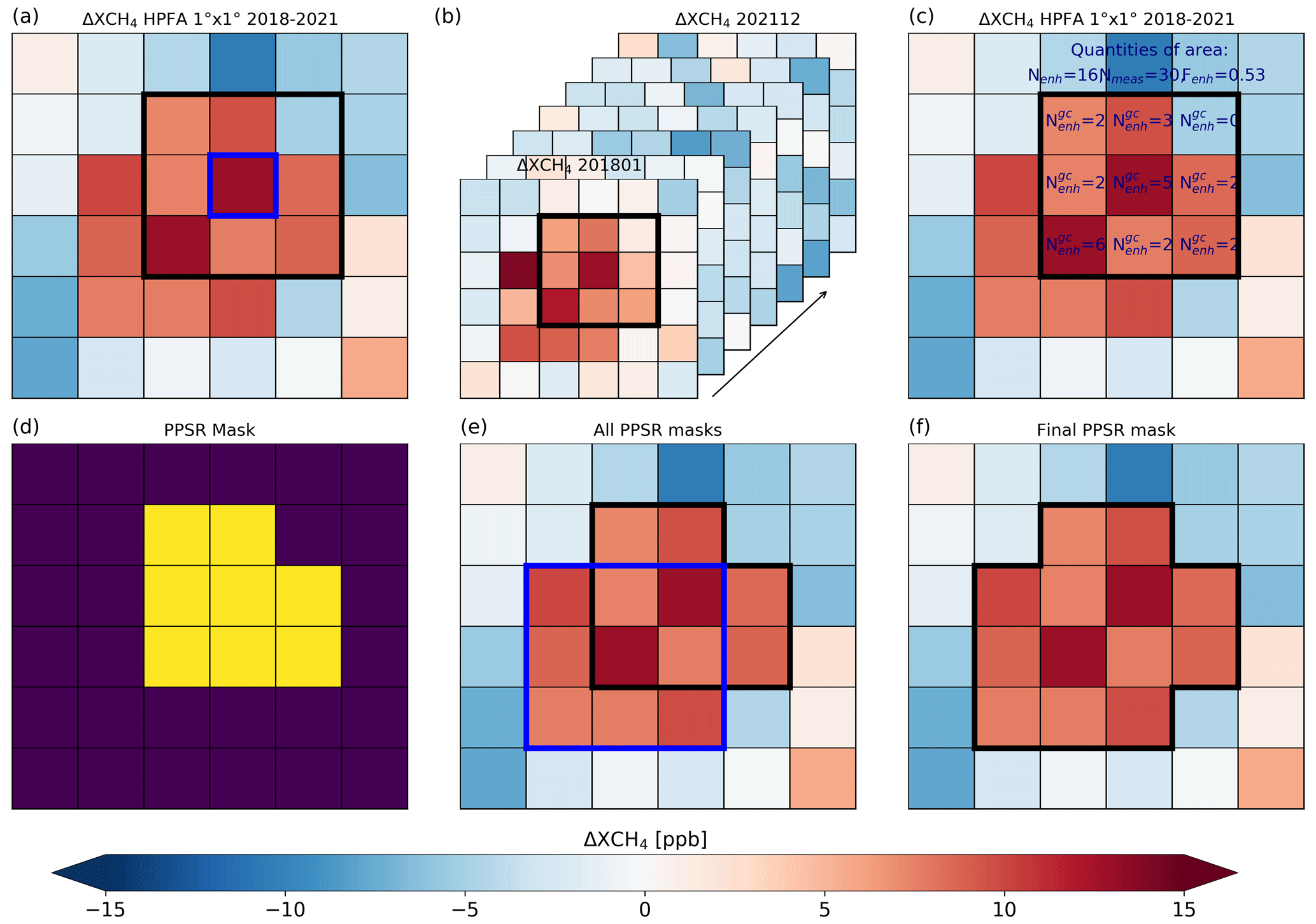
Figure 5 Illustration of the process to identify a potential persistent source region (PPSR). (a) 2018–2021 ΔXCH₄ calculated with an HPFA of 1°×1°. The detection process is illustrated for the blue-outlined grid cell. First, an area of 3×3 grid cells (outlined in black) is defined around the grid cell considered. (b) Next, the anomalies within the black-outlined area are analyzed for all monthly ΔXCH₄ and σ maps from 2018 to 2021 to calculate N_meas, N_enh and $F_{\mathrm{enh}}=N_{\mathrm{enh}}/N_{\mathrm{meas}}$ (definition in Sect. 3.3.2). In addition, for each grid cell within the 3×3 area, $N_{\mathrm{enh}}^{\mathrm{gc}}$ is counted. (c) Multi-year ΔXCH₄ with the results from the analysis described in (b). In each grid cell in the black-outlined area, $N_{\mathrm{enh}}^{\mathrm{gc}}$ is shown. The 3×3 area fulfills the conditions for a PPSR from Eq. (3), since F_enh≥0.5, N_meas≥16 and $N_{\mathrm{enh}}^{\mathrm{gc}}$ of central grid box ≥1. (d) Resulting mask (yellow grid cells) of the detected PPSR. Only the grid cells that have an enhanced anomaly in at least 1 month are considered for the mask ($N_{\mathrm{enh}}^{\mathrm{gc}}>\mathrm{0}$). (e) Multi-year ΔXCH₄ with all detected PPSR masks in that region. The algorithm is applied to each grid cell, resulting in an additional PPSR being detected (outlined in blue). (f) Multi-year ΔXCH₄ with the final PPSR mask, which is created by merging PPSRs that are directly adjacent or overlapping.

We have chosen $F_{\mathrm{enh},\min }=\mathrm{0.5}$ for the following reasons. Persistent methane sources do not always show enhanced methane anomalies in all months. For example, some sources such as wetlands or rice paddies show seasonal variations in emissions. Emissions from coal mines can also vary over time, as they depend on mining activity. In addition, we also want to take into account persistent sources in the detection process that started emitting during 2018–2021 and therefore do not show emissions over the entire period. With $N_{\mathrm{meas},\min }=\mathrm{16}$, we also take into account regions that do not contain data in all 48 months.

3.3.2 Mask potential persistent source regions

To detect PPSRs in an anomaly dataset, we define small areas around every grid cell of the dataset and calculate for each of those areas the number of months with at least one anomaly, N_meas; the number of months with enhanced anomalies, N_enh; and the fraction of months with enhanced anomalies, F_enh, by analyzing the monthly XCH₄ and σ maps from 2018 to 2021. In detail, for each grid cell, we apply the following steps, which are illustrated in Fig. 5. We first define an area of 3×3 grid cells consisting of the grid cell itself and the directly adjacent grid cells (black-outlined area in Fig. 5a). We are using a small 3×3 area for the calculation of N_meas, N_enh and F_enh rather than only analyzing a single grid cell for the following reason. The ΔXCH₄ enhancements within a persistent source region depend on the source itself and on the meteorological conditions. Therefore, enhancements show temporal and spatial variability. Consequently, the ΔXCH₄ enhancements can occur at different grid cells in different months of the persistent source region. To account for this in the detection process, we analyze the ΔXCH₄ and σ maps of multiple grid cells simultaneously rather than considering each grid cell independently. We use an area of 3×3 to take into account the fact that the varying meteorological situations in the monthly XCH₄ maps are not as strong as in the daily XCH₄ data. In the monthly maps, the daily plumes, which vary with wind strength and direction, typically average out and result in a XCH₄ enhancement over the source region, which shows only slight monthly variability.

After defining the 3×3 area, we analyze all monthly ΔXCH₄ and σ maps from 2018 to 2021 for the 3×3 area to calculate N_meas, N_enh and F_enh (Fig. 5b and c). We also count the number of months, $N_{\mathrm{enh}}^{\mathrm{gc}}$, in which the anomaly in the grid cell is enhanced for each grid cell in the 3×3 area. If the 3×3 area fulfills the persistence conditions from Eq. (3) and if the center grid cell shows an enhanced anomaly in at least 1 month, we mask the area as PPSR (yellow area in Fig. 5d). To label a 3×3 area as PPSR, we mark all grid cells within the area that show an enhanced anomaly in at least 1 month ($N_{\mathrm{enh}}^{\mathrm{gc}}\ge \mathrm{1}$). Thus, grid cells with F_enh<0.5 can also be part of a PPSR if their enhancements contribute to the 3×3 area being marked as a PPSR. We only consider 3×3 areas that have no complicated topography (median of surface roughness <80 m and standard deviation of the surface elevation <150 m) as PPSRs. As can be seen in Fig. 5c, the analysis of an area rather than a single grid cell enables the detection of source regions in which the individual grid cells show no persistent enhancement, but the area does. This means that the enhanced anomalies need not occur at the same grid cell every month but can vary monthly within the area.

PPSRs that are directly adjacent or overlapping are merged into one PPSR (Fig. 5e and f). For this, we apply a labeling algorithm in which each individual PPSR is assigned its own number, with directly adjacent or overlapping PPSRs getting the same number. In the end, we get a global map containing the separated and labeled PPSRs of the anomaly dataset considered.

We apply the detection process to the five anomaly datasets and obtain five global maps with the detected PPSRs.

3.3.3 Refinement of PPSR masks

The detected PPSR masks describe the locations and shapes of the corresponding source regions. However, some of the masks do not cover the entire spatial extent of the source regions. Therefore, in the next step, we refine the PPSR masks. One example is shown in Fig. 6a. It can be seen that the two PPSR masks do not contain all the grid cells that would be identified by eye as part of the source regions because their fractions F_enh do not exceed the threshold $F_{\mathrm{enh},\min }=\mathrm{0.5}$ required for detection (Eq. 3). These grid cells are nevertheless part of the source region since they have a high fraction of F_enh and are located in the immediate surroundings of the source regions. To add them to the source regions, we could lower the F_enh,min parameter. But this would imply a change in the persistence condition. To determine the total spatial extent of the source regions without changing the persistence condition, we choose the following approach. We add grid cells to the PPSR masks that are in the immediate vicinity and whose fractions F_enh indicate that they are part of the source. For this, we identify all grid cells with F_enh≥0.33 that also fulfill all other conditions from Eq. (3). We refer to these grid cells as “toseeds” (green grid cells in Fig. 6b). The grid cells detected with $F_{\mathrm{enh},\min }=\mathrm{0.5}$ are called seeds (yellow grid cells in Fig. 6b). We chose 0.33 as the lower threshold, since F_enh≥0.33 indicates that the grid cells show enhanced anomalies in a certain number of months and are therefore still strongly influenced by the sources within the PPSR, although its F_enh is smaller than 0.5. Grid cells with F_enh<0.33 indicate a weaker influence of the sources on the grid cells, which is why we did not include them in the refining process. Next, we apply a random walker algorithm (Grady, 2006) to assign the toseeds to the seeds. A random walker algorithm is an image segmentation algorithm, which can divide an image into several sections based on threshold values. A first threshold is used to define the pixels of the image that represent the foreground of the image and are called seeds (the grid cells detected with F_enh,min). The seeds can have different labels so that the foreground can be divided into different areas. With a second threshold, which is below the first one, the pixels of the background that are not to be considered further are defined. The pixels between the first and second threshold are the so-called undefined pixels that the random walker algorithm assigns to the corresponding seeds using a diffusion equation (the grid cells with $\mathrm{0.33}\le F_{\mathrm{enh}}\le \mathrm{0.5}$). Based on the gradient between an undefined pixel, the different seeds and the distance between them, the probability of which seed the respective undefined pixel is assigned is calculated. The lower the gradient, i.e., the more similar the values of the undefined pixel and a seed are, the higher the probability that this pixel will be assigned to this seed. Undefined pixels that do not have a contiguous path to at least one seed are discarded. As the basis on which the grid cells detected with F_enh,min are assigned to the PPSRs, we use the multi-year (2018–2021) ΔXCH₄ of the analyzed anomaly dataset. Figure 6c shows the mask created by assigning the toseeds to the seeds. It can be seen that the spatial extent of the source regions is now better described by the masks and that grid cells connecting the separate source regions are added. But some of the toseeds have a low multi-year ΔXCH₄ mean compared to the seeds. Here, we only want to consider toseeds that have comparable high multi-year ΔXCH₄ as part of the source region and remove added toseeds with ΔXCH₄ smaller than 25 % of the maximum ΔXCH₄ of the seeds. In the end, we obtain the refined PPSR masks, which now describe the spatial extent of the source regions better (Fig. 6d). We emphasize that the example shown in Fig. 6, in which two PPSRs are first merged and then separated, does not appear often. We only used it to illustrate all the steps of the refinement process for one region. Due to the refinement, the number of final PPSRs can differ from the number of PPSRs detected in Sect. 3.3.2. On the one hand, multiple PPSRs can be combined into one PPSR by adding new grid cells to the masks. On the other hand, a PPSR can be split into multiple PPSRs by removing grid cells with 2018–2021 ΔXCH₄ means that are too low. We apply the refinement to each of the five global maps containing the detected PPSRs (Sect. 3.3.2).

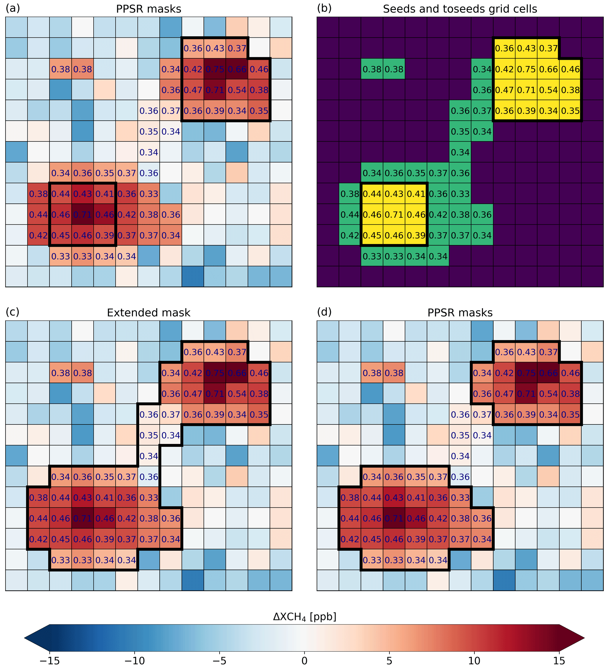
Figure 6 Illustration of the process to refine PPSR masks. (a) Multi-year (2018–2021) ΔXCH₄. In each grid cell, the fraction F_enh is shown, which is calculated for the 3×3 area of the respective grid cell (see Sect. 3.3.2). Grid cells that do not contain a fraction do not fulfill any of the persistence conditions from Eq. (3). The detected PPSRs (black-outlined) are the result of the detection process described in Sect. 3.3.2. Some grid cells with F_enh<0.5 and a high multi-year ΔXCH₄ mean would be assigned by eye as part of the source region. To add them to the masks we use the following steps. (b) First, we mark all toseeds (shown in green, definition in Sect. 3.3.3). The seeds are shown in yellow. (c) The toseeds are assigned to the seeds using a random walker algorithm. (d) In the final step, the grid cells with a multi-year ΔXCH₄ mean less than 25 % of the maximum multi-year ΔXCH₄ mean within the mask are removed from the mask. The final masks describe the refined PPSRs.

3.3.4 Filtering of potential false positives

Much effort was made to minimize systematic biases when generating the WFMD v1.8 XCH₄ data product (Schneising et al., 2023). However, it is not guaranteed that the WFMD v1.8 product is entirely unbiased. This means that despite the good quality of the product, it is not certain that every individual XCH₄ enhancement has its origin in a real methane source. For example, localized XCH₄ enhancements could be caused by scenes with inhomogeneous albedo (e.g., coastal regions, lakes and rivers) and complex topography. To take this into account, the PPSRs are filtered for surface features that could potentially lead to a false positive detection. We use a conservative approach and prefer to accept false negatives rather than false positives. We decide whether a PPSR has challenging surface features based on the following properties: the correlation between SWIR surface albedo and XCH₄, the standard deviation of the surface elevation within the PPSR mask, the frequency of months in which the largest XCH₄ enhancements occur in or adjacent to grid cells with high surface roughness, the fraction of coastal grid cells in the PPSR mask, and the frequency of months in which the largest XCH₄ enhancements occur over or next to water grid cells. If a PPSR is identified by one of these criteria, then it is filtered and not considered further. Excluded from this are PPSRs in which very strong XCH₄ enhancements occur. By this, we ensure that important source regions are not excluded due to their surface features. As we focus in this study on source regions that contribute significantly to the global methane budget, we filter out PPSRs with weak XCH₄ enhancements. Additionally, we filter out PPSRs that occur in the Bodélé Depression in Chad. This is a region where strong dust storms occur on average 100 d yr⁻¹, always directed towards the southwest and with a plume-like structure. Analyses of the WFMD data product have shown that these special conditions, which only occur in this region, can lead to false-positive detections. We apply the filtering to each detected PPSR of each anomaly dataset to obtain five global maps comprising the refined and filtered PPSR masks.

3.4 Combination of PPSRs from different anomaly datasets

We used five different HPFA(n) for the calculation of the ΔXCH₄ maps to detect source regions of various sizes (see Sect. 3.2). As a result, we identified different PPSRs in each anomaly dataset. To consider all PPSRs collectively, we combine them into one global map. For this, we must take into account the fact that the same source region can be detected in multiple anomaly datasets and is thus described by more than one mask. In such a case, we merge all detected masks of the PPSR into one new mask. An example of the combination process is illustrated in Fig. 7. Here we show the well-known source regions in South Sudan (see Sect. 3.2), which we detect in the HPFA(4°) and HPFA(5°) anomaly datasets, and the combined masks of the individual source regions. Finally, we obtain one global map, in which each detected source region is described by one mask. The masks of some PPSRs are shown in Fig. 8, including some well-known source regions such as the oil and gas fields in the Permian Basin in the USA (Schneising et al., 2020; Zhang et al., 2020; Varon et al., 2023; Veefkind et al., 2023), the natural gas fields Galkynysh and Dauletabad in Turkmenistan (Schneising et al., 2020), and the coal mining area in the Bowen Basin in Queensland in Australia (Sadavarte et al., 2021).

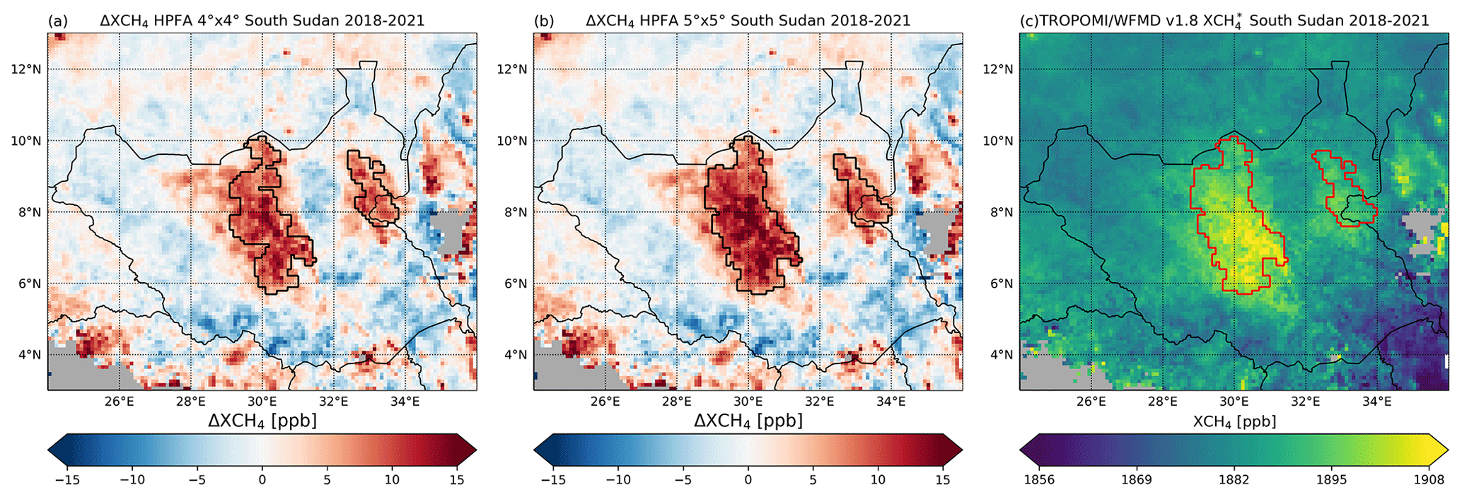
Figure 7 Example of PPSRs detected in two different anomaly datasets. (a) Multi-year (2018–2021) ΔXCH₄ of the South Sudan region calculated with an HPFA of 4°×4°. The detected PPSRs (outlined in black) have already been filtered (see Sect. 3.3.4). (b) Same as (a) but for an HPFA of 5°×5°. (c) Corresponding 2018–2021 XCH₄. The final PPSR masks of the combined masks from different anomaly datasets.

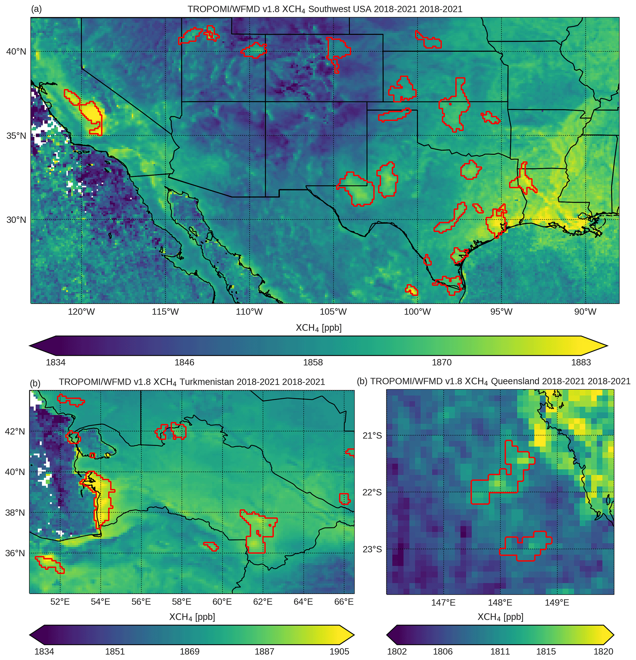
Figure 8 Final PPSR masks (outlined in red) after the filtering (Sect. 3.3.4) and combining (Sect. 3.4) processes, shown for several regions of the world. (a) 2018–2021 XCH₄ for the southwestern part of the USA and northern Mexico. Some of the PPSRs are located in well-known oil and gas basins like the Permian, Anadarko, Barnett, Haynesville, Denver and San Joaquin basins. (b) Same as (a) but for Turkmenistan, parts of Iran, Uzbekistan and Kazakhstan. One of the detected PPSRs includes two of the largest natural-gas fields in the world, Galkynysh and Dauletabad. (c) Same as (a) but for parts of Queensland in Australia. Two PPSRs located in the Bowen Basin, a well-known coal mining area, are detected.

3.5 Emission estimation

To compute emission estimates for each of the detected PPSRs, we apply the fast data-driven method of Buchwitz et al. (2017). This method is designed to calculate averaged long-term emission estimates from time-averaged XCH₄ maps. It uses a conversion factor to convert an XCH₄ enhancement over a source region into an emission estimate. This implies the assumption that emissions from an isolated source result in an XCH₄ enhancement, δXCH₄, over the source region compared to the surrounding region. To determine the monthly emission estimate, E (Mt yr⁻¹), of a PPSR, we apply the method to the monthly averaged XCH₄ maps using the following equation:

$$\begin{array}{}\text{(4)}& E=\mathit{\delta }{\mathrm{XCH}}_{\mathrm{4}}\cdot M\cdot M_{\exp }\cdot L\cdot V\cdot \mathrm{2}.\end{array}$$

The δXCH₄ (ppb) describes the XCH₄ enhancement of the PPSR and is calculated by computing the difference in the mean XCH₄ over the source region from the mean XCH₄ over the surrounding region. The surrounding region is defined as described in Fig. 9. We only consider the grid cells in the surrounding region that are not part of other PPSRs in the surrounding region. We estimate the emissions only if the PPSR as well as the surrounding region are each filled with at least 25 % data. To convert the mole fraction change in δXCH₄ over the source region into a methane mass change per area, M and M_exp are used. M ($\mathrm{5.345}\times {\mathrm{10}}^{-\mathrm{9}}{\mathrm{MtCH}}_{\mathrm{4}}{\mathrm{km}}^{-\mathrm{2}}{\mathrm{ppb}}^{-\mathrm{1}}$) is the methane mixing ratio enhancement to mass enhancement conversion factor for standard conditions, i.e., for a surface pressure of 1013.25 hPa. Since the actual mass change M_i of the ith grid cell depends on the surface pressure p_i (hPa) of the grid cell, Buchwitz et al. (2017) additionally used the dimensionless conversion factor M_exp, which is defined as

$$\begin{array}{}\text{(5)}& M_{\exp }={\displaystyle \frac{<M_i>}{M}}\approx {\displaystyle \frac{<p_i>}{\mathrm{1013.25}}}\approx <e^{-z_i/H}>,\end{array}$$

with surface elevation z_i (km) of the ith grid cell, the scale height H (8.5 km) and $<>$ denoting the mean over all grid cells of the source region. L (km) in Eq. (4) is the effective length of the source region, which we calculate as the square root of the PPSR size. V (km yr⁻¹) is the wind speed from Sect. 2.2 averaged over the source region. The reason for adding factor 2 is described in detail in Buchwitz et al. (2017) but is briefly explained in the following. When an air parcel travels with constant wind speed across the source region, it accumulates methane, which results in an XCH₄ enhancement when it exits the source region (δXCH_4,exit). However, δXCH₄ from Eq. (4) describes the mean XCH₄ enhancement over the source region and not δXCH_4,exit. Assuming a linear XCH₄ increase while traveling across the source region (see Fig. 3 in Buchwitz et al., 2017), these two enhancements are linked via $\mathit{\delta }{\mathrm{XCH}}_{\mathrm{4}}=\mathrm{0.5}\cdot \mathit{\delta }{\mathrm{XCH}}_{\mathrm{4},\mathrm{exit}}$. Therefore, the δXCH₄ has to be multiplied by 2 to describe the XCH₄ enhancement of the air parcel that results from the emission of the source region.

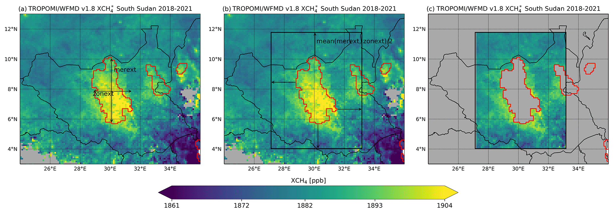
Figure 9 Illustration of the automated calculation of the surrounding area for a PPSR. (a) 2018–2021 XCH₄. The detected and unfiltered PPSRs in the HPFA(5°) anomaly dataset for the South Sudan region are shown (outlined in red). The surrounding region for the central PPSR is calculated as follows. First the maximum extents of the PPSR in the meridional (merext) and zonal (zonext) directions are calculated. (b) Next, a rectangle (black-outlined area) is defined around the PPSR by expanding the northernmost, southernmost, westernmost and easternmost coordinates by L_surr, which is half of the mean of merext and zonext. If L_surr is smaller than 0.5°, we set it to 0.5° to provide a reasonable size of the surrounding region. (c) In the last step, all grid cells outside the rectangle and all grid cells inside the source region are removed. The grid cells with XCH₄ are defined as the surrounding area of the central PPSR.

We calculate the 1σ uncertainty in the monthly emission estimate E, u_E, by computing the sum of the squared uncertainties in the XCH₄ enhancement, $u_{\mathit{\delta }{\mathrm{XCH}}_{\mathrm{4}}}$, and the wind speed, u_v, with respect to their mean values via

$$\begin{array}{}\text{(6)}& {\left({\displaystyle \frac{u_E}{E}}\right)}^{\mathrm{2}}={\left({\displaystyle \frac{u_{\mathit{\delta }{\mathrm{XCH}}_{\mathrm{4}}}}{\mathit{\delta }{\mathrm{XCH}}_{\mathrm{4}}}}\right)}^{\mathrm{2}}+{\left({\displaystyle \frac{u_v}{V}}\right)}^{\mathrm{2}}.\end{array}$$

We calculate $u_{\mathit{\delta }{\mathrm{XCH}}_{\mathrm{4}}}$ by varying the size of the surrounding region and calculating the standard deviation of the resulting δXCH₄ enhancements. We vary the region by adding to the northernmost, southernmost, westernmost and easternmost coordinates of the surrounding region all possible combinations of 0 and 2×L_surr, where L_surr is the length used to define the surrounding region (see Fig. 9). The square of the uncertainty in the wind is the sum of the squared standard deviation of the monthly wind speeds within the source region and the squared mean of the standard deviations of the wind speeds within the months for each grid cell.

We calculate the averaged long-term emission estimate $\stackrel{\mathrm{‾}}{E}$ of a PPSR by averaging all monthly emission estimates for the period 2018–2021. For the corresponding uncertainty in the long-term emission estimate we use error propagation by computing the ratio of the root of the sum of the squared monthly uncertainties u_E and the effective number of months n_eff contributing to the mean estimate,

$$\begin{array}{}\text{(7)}& u_{\stackrel{\mathrm{‾}}{E}}={\displaystyle \frac{\sqrt{{\sum }_j{u}_{E,j}^{\mathrm{2}}}}{n_{\mathrm{eff}}}}.\end{array}$$

With n_eff, we consider the correlation between the monthly emission estimates. n_eff equal to 1 means that all emission estimates are correlated, and n_eff equal to the total number of emission estimates means that all emission estimates are uncorrelated. We choose n_eff with the assumption that the blocks of quarter-yearly emission estimates are uncorrelated. n_eff is therefore the number of quarter-yearly data blocks in which at least one emission estimate contributes to the mean.

3.6 Assignment to source type

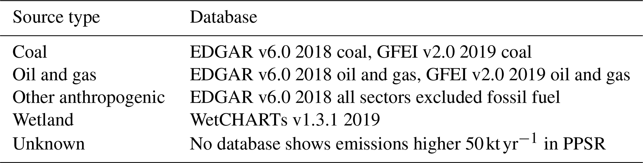
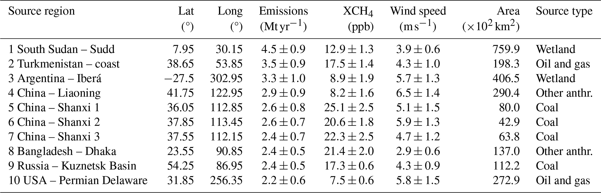
To determine the dominant methane source type in the detected PPSRs, we compare sector-specific emissions from different emission databases. We distinguish between the source types coal, oil and gas, other anthropogenic sources, wetlands, and unknown (see Table 1). We use the emission data regarding coal and oil and gas from EDGAR v6.0 2018 and GFEI v2.0 2019 (Sect. 2.4). To determine the emissions originating from other anthropogenic sources, we use anthropogenic methane emissions from all sectors, excluding fossil fuel from EDGAR v6.0 2018. For wetland emissions, we use the ensemble of WetCHARTs v1.3.1 for 2019 (Sect. 2.4). We assign the source type with the highest emissions as the dominant source type of the corresponding PPSR. For this, we sum up the emissions in the PPSR for each source type using an expanded PPSR mask, which includes the directly adjacent outer grid cells to account for variations in the locations of the sources in the databases. We assign the type unknown to a PPSR if the total emissions in the respective PPSR mask are less than 50 kt yr⁻¹ for all three emission databases. It should be noted that no uncertainties are specified in the databases used, which means that the uncertainties cannot be considered in the source type assignment. Therefore, we have only taken into account possible uncertainties in the databases in the sense of underestimation of emissions, by setting the threshold value to be exceeded for source type assignment (50 kt yr⁻¹) to be significantly lower than the lowest mean emissions estimate of 2018–2021 detected by us (120 kt yr⁻¹). With 50 kt yr⁻¹, however, we also ensure that the databases have a certain minimum emission level when assigning a PPSR to a source type.

Table 1 Dominant source types of PPSRs and the corresponding databases used to estimate the sector-specific emissions.

4 Results

In this section, we present the results of the PHD algorithm, which we use to detect potential persistent source regions (PPSRs). We provide a global overview of the detected PPSRs by describing the distribution of the PPSRs among the different source types: coal, oil and gas, other anthropogenic sources, and wetlands, as well as a rough total emission estimate of all the detected PPSRs (Sect. 4.1). We then analyze the 10 PPSRs with the highest emission estimates in more detail (Sect. 4.2). These include the Sudd Wetlands in South Sudan (Sect. 4.2.1), the west coast of Turkmenistan (Sect. 4.2.2), the Iberá Wetlands in Argentina (Sect. 4.2.3), several regions in China (Sect. 4.2.4 and 4.2.5), the city of Dhaka in Bangladesh and its surrounding area (Sect. 4.2.6), the Kuznetsk Basin in Russia (Sect. 4.2.7), and the Permian Basin in the United States (Sect. 4.2.8).

4.1 Global overview

We applied the PHD algorithm as described in Sect. 3 and detected a total of 217 PPSRs, whose global distribution and assigned source types are shown in Fig. 10. Based on the comparison of the emission databases, the fraction of dominant source types is 7.8 % coal, 7.8 % oil and gas, 30.4 % other anthropogenic sources, 7.3 % wetlands, and 46.5 % unknown.

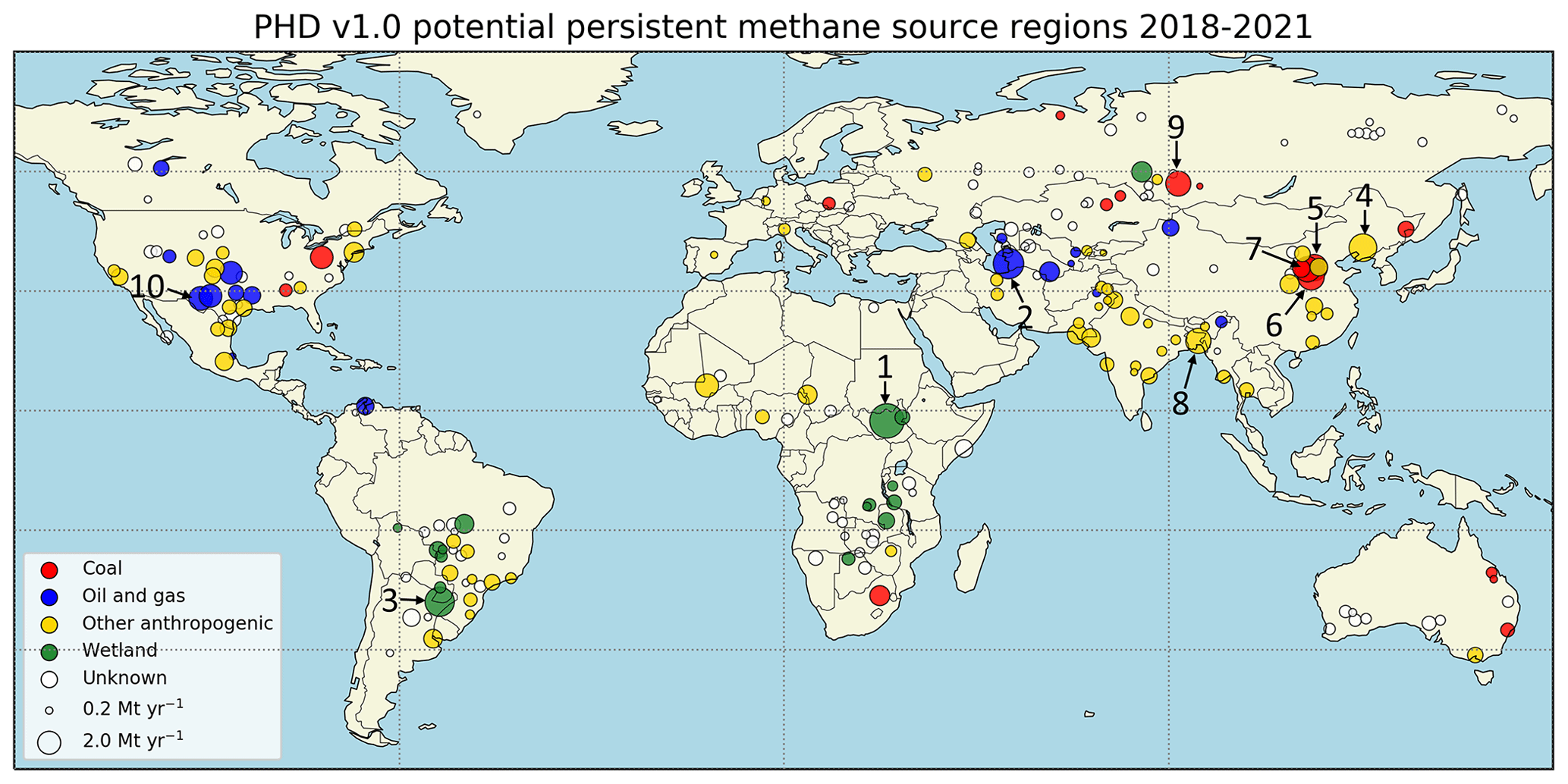
Figure 10 All PPSRs detected with the PHD algorithm grouped by the different dominant source types. The sizes of the circles scale with the emission estimates of the PPSRs for 2018–2021. The 10 PPSRs with the highest emission estimates are indicated by a number.

Some of the detected source regions are well-known coal production sites, which already have been subject of several studies, such as the region of Shanxi in China (Chen et al., 2022), the Bowen Basin in Queensland in Australia (Sadavarte et al., 2021) and the Upper Silesia Coal Basin in Poland (Tu et al., 2022). Other PPSRs related to coal mining activities include the Kuznetsk Basin in Russia, regions in and around Johannesburg in South Africa, the Appalachian Coal Basin in the United States, and the Ekibastuz Coal Basin in Kazakhstan. We also detect several PPSRs located in known oil and gas basins including the Permian (Schneising et al., 2020; Zhang et al., 2020; Varon et al., 2023; Veefkind et al., 2023), Uintah (de Gouw et al., 2020), Haynesville (Shen et al., 2022) and Anadarko basins (Schneising et al., 2020) in the USA, as well as two of the world's largest natural-gas fields, Galkynysh and Dauletabad in Turkmenistan (Schneising et al., 2020). A large number of the detected PPSRs are assigned to the source type other anthropogenic sources. These include regions used for agriculture, such as the Po Valley in Italy, and regions including large cities, such as Dhaka in Bangladesh, Mumbai and Delhi in India, Madrid in Spain, Buenos Aires in Argentina, and Rio de Janeiro in Brazil. The emissions in these cities can originate from anthropogenic sources of different types. For example, Maasakkers et al. (2022) analyzed the methane emissions of several cities, including Mumbai, Delhi and Buenos Aires, and showed that landfills contribute a large amount to the total emissions of these cities. In addition to anthropogenic source regions, we also detected PPSRs in wetland regions. These include well-known methane source regions like the Sudd Wetlands in South Sudan (Pandey et al., 2021), the Pantanal Wetlands in Brazil and the wetlands formed by the Paraná River in Argentina (Parker et al., 2018). Often, source regions contain multiple sources of different types, which is not indicated in the global map of Fig. 10. For example, we identified a source region at Lake Chad where the emission databases indicate strong anthropogenic emissions but also strong wetland emissions. Another example is a source region in the Central Valley in the USA, which is an oil and gas production site but is also known for its livestock farming (Buchwitz et al., 2017). Moreover, 46.5 % of the identified PPSRs are not assigned to any source type. By analyzing these in more detail, we find that most of them occur in regions with wetlands but in which WetCHARTs v1.3.1 shows emissions lower than the threshold of 50 kt yr⁻¹, which needs to be exceeded to assign a PPSR to the corresponding source type (see Sect. 3.6). For example, we detected four PPSRs in Zambia, which are all known wetland methane source regions (Shaw et al., 2022), but only one of them was categorized as the wetland type, while the others were assigned to the unknown type. We also detected some unknown PPSRs that are located in fossil fuel production regions, such as the Cesar–Ranchería Basin in Colombia or the Surat Basin in Queensland, and some unknown PPSRs in urban areas, such as in Tulsa (USA) or in Calgary (Canada). As reported in Foy et al. (2023), the emissions from urban areas are often underestimated in EDGAR, which may be the reason that these PPSRs could not be assigned to the other anthropogenic type.

The sum of the 2018–2021 mean emission estimates of all detected PPSRs is approximately 150 Mt yr⁻¹, of which 13.0 % are associated with emissions from the coal source type, 12.5 % from the oil and gas type, 35.4 % from the other anthropogenic type, 11.9 % from the wetland type, and 27.2 % from the unknown type. We compared our total emission estimates with the calculated bottom-up methane budget for 2017 from Saunois et al. (2020). The detected PPSRs account for 20.1 % of the total bottom-up emissions (747 Mt yr⁻¹), for 24.1 % of the emissions related to anthropogenic sources (380 Mt yr⁻¹) and for 4.9 % of the emissions related to natural sources (367 Mt yr⁻¹). An analysis of the anthropogenic emissions shows that the PPSRs assigned to fossil fuel account for 28.4 % of the total fossil fuel emissions (135 Mt yr⁻¹) reported in Saunois et al. (2020), describing 44.5 % of coal-related emissions (44 Mt yr⁻¹) and 22.3 % of oil and gas-related emissions (84 Mt yr⁻¹). The other anthropogenic PPSRs account for 21.8 % of the bottom-up anthropogenic emissions that are not related to fossil fuel (245 Mt yr⁻¹). Compared to Lauvaux et al. (2022) and Schuit et al. (2023), the emissions of our source regions account for a larger percentage of the reported anthropogenic emissions. The oil and gas methane ultra-emitters detected by Lauvaux et al. (2022) account for 8 %–12 % of the oil and gas emissions reported by national inventories. In Schuit et al. (2023), anthropogenic super-emitters are detected, accounting for 2.7 % of the total anthropogenic emissions reported by Saunois et al. (2020). In addition to the different methodology and data product, the higher percentage of emissions detected in our study can be explained by the focus on persistent methane sources and the additional consideration of larger-scale source regions rather than only detecting point sources.

We only detected a fraction of the total global emissions because we only considered source regions that are localized and have a persistent enhancement that is above a threshold. In addition, the sources can only be detected if sufficient TROPOMI measurements are available, which depends, for example, on the presence of clouds in the region considered. Thus, emissions from sources that do not meet these criteria, such as source regions that only show strong emissions in 1 of the 4 years, cannot be detected with this method. For the calculation of the total emissions, we have to consider that a few of the detected PPSRs could be false positives, even though we applied a filter to PPSRs in Sect. 3.3.4. If some of the PPSRs are false positives, then the calculated total emissions are overestimated.

Figure 11 shows the distribution of the 2018–2021 mean emission estimates of all detected PPSRs and the corresponding cumulative distribution. The majority of the detected PPSRs, 63.6 %, have a mean emission estimate between 0.1 and 0.6 Mt yr⁻¹. Although the PPSRs with emission estimates greater than 0.6 Mt yr⁻¹ account for only 36.4 % of the detected PPSRs, they are responsible for 66.8 % of the total detected emission estimates. Most of the PPSRs with a higher emission estimate than 0.6 Mt yr⁻¹ were assigned to a source type, which indicates that the emission databases also report enhanced methane emissions in the corresponding regions. In contrast, 64.5 % of the PPSRs with emission estimates below 0.6 Mt yr⁻¹ are assigned to the unknown source type, which accounts for 88.1 % of all unknown PPSRs. In general, the shape of the distribution is in agreement with other studies describing a heavy-tailed distribution of strongly emitting methane emitters (Frankenberg et al., 2016; Jacob et al., 2016; Lauvaux et al., 2022; Zavala-Araiza et al., 2015).

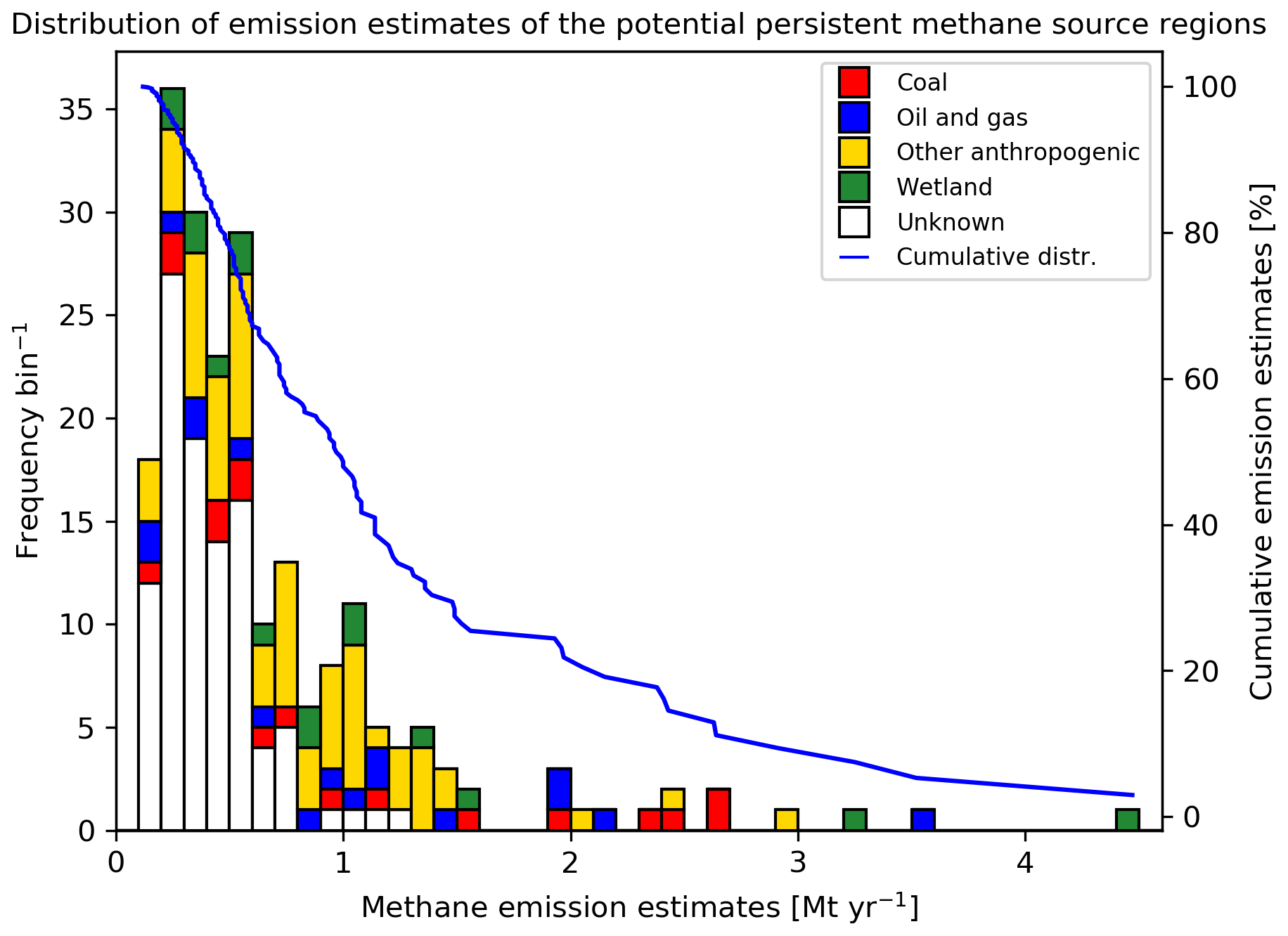
Figure 11 Distribution of the 2018–2021 emission estimates of the detected PPSRs, as well as the corresponding cumulative distribution (blue line). The frequency per 0.1 Mt yr⁻¹ bin associated with the distribution of the emission estimates is shown on the left y axis, and the percentage share of the cumulative emission estimate of the total emission estimate is shown on the right y axis. In each bin, the source types of the PPSRs contributing to that bin are shown in the corresponding colors.

For several of the detected PPSRs the emission estimates show good agreement with the emissions quantified in other studies. These include, for example, the Upper Silesia Coal Basin in southern Poland and the Bowen Basin in Queensland in Australia. The Upper Silesia Coal Basin in Poland is one of Europe's strongest methane emission hotspots due to its intense coal mining activities. For the PPSR in this area, we calculate an emission estimate of $\mathrm{0.59}\pm \mathrm{0.11}\mathrm{Mt}{\mathrm{yr}}^{-\mathrm{1}}$, which is in good agreement with the emissions calculated in Tu et al. (2022) of $\mathrm{0.50}\pm \mathrm{0.02}\mathrm{Mt}{\mathrm{yr}}^{-\mathrm{1}}$ for the period from November 2017 to December 2020 and with the emissions quantified using methane observations conducted from aircraft measurements in June 2018 during the CoMet (Carbon Dioxide and Methane Mission) campaign of $\mathrm{0.44}\pm \mathrm{0.14}\mathrm{Mt}{\mathrm{yr}}^{-\mathrm{1}}$ and $\mathrm{0.48}\pm \mathrm{0.13}\mathrm{Mt}{\mathrm{yr}}^{-\mathrm{1}}$ (Fiehn et al., 2020; Fix et al., 2018). Another well-known methane source region is the Bowen Basin in Queensland in Australia, which is a coal mining area. Here we detected two PPSRs for which the combined emission estimate is $\mathrm{0.63}\pm \mathrm{0.16}\mathrm{Mt}{\mathrm{yr}}^{-\mathrm{1}}$ for 2018–2021, which also agrees well within the uncertainties with the calculated emissions in Sadavarte et al. (2021) of $\mathrm{0.57}\pm \mathrm{0.10}\mathrm{Mt}{\mathrm{yr}}^{-\mathrm{1}}$ for 2018–2019.

Table 2 Summary of the results of the 10 PPSRs with the highest methane emission estimates detected by the PHD algorithm for 2018–2021. The ± represents the corresponding uncertainty in the long-term emission estimate calculated via Eq. (7).

4.2 PPSRs with the highest emission estimates

An overview of the results of the 10 PPSRs with the highest emission estimates is summarized in Table 2. In the following, each PPSR is discussed in detail, including the 2018–2021 time series for the emission estimates; XCH₄ enhancements and mean wind speed; and a comparison of the results with the emissions from EDGAR v6.0, GFEI v2.0, WetCHARTs v1.3.1, and related studies.

4.2.1 South Sudan – Sudd Wetland

The PPSR with the highest emission estimate for 2018–2021, called PPSR 1, is detected in the Sudd in central South Sudan, one of the world's largest wetlands. South Sudan, and in particular its wetland region, is a well-known methane source region that has been subject of several studies (Frankenberg et al., 2011; Hu et al., 2018; Lunt et al., 2019; Pandey et al., 2021). By comparing the emission databases within PPSR 1 as described in Sect. 3.6, we determine its dominant source type as wetland, which corresponds to its location in the Sudd. In Fig. 12 we show an overview of the PPSR 1 results. Figure 12a shows the 2018–2021 XCH₄ of the South Sudan region, including the detected PPSR 1 mask, as well as one other identified PPSR in eastern South Sudan. It can be seen that the XCH₄ within PPSR 1 is strongly enhanced compared to its surroundings. The area outlined in black in Fig. 12a indicates the surrounding region, which is used to calculate the XCH₄ enhancements δXCH₄ of PPSR 1 (see Sect. 3.5). The corresponding time series of the δXCH₄ for 2018–2021 is shown in Fig. 12c. The mean for the entire time period is 12.9±1.3 ppb, and the standard deviation is 10.3 ppb. The δXCH₄ shows a seasonal cycle with its peak enhancement at the end of each year, as well as a strong increase since the end of 2020. Due to the frequent occurrence of clouds during the wet season from April to November, only a few days with data are available for this period of the year. In Fig. 12b we show the emission estimates of PPSR 1 for 2018–2021, which we calculated as described in Sect. 3.5. The mean of the emission estimates is $\mathrm{4.5}\pm \mathrm{0.9}\mathrm{Mt}{\mathrm{yr}}^{-\mathrm{1}}$, where ± indicates the long-term emission estimate uncertainty calculated via Eq. (7). By comparing the time series in Fig. 12b–d, it can be seen that due to the small variations in the mean wind speed V, the δXCH₄ variations determine the temporal variations in the emission estimates, including the strong increase since the end of 2020. This strong increase is in good agreement with the finding that tropical wetlands are a major contributor to the strong methane growth rate in 2020 and 2021 (Peng et al., 2022; Lin et al., 2023).

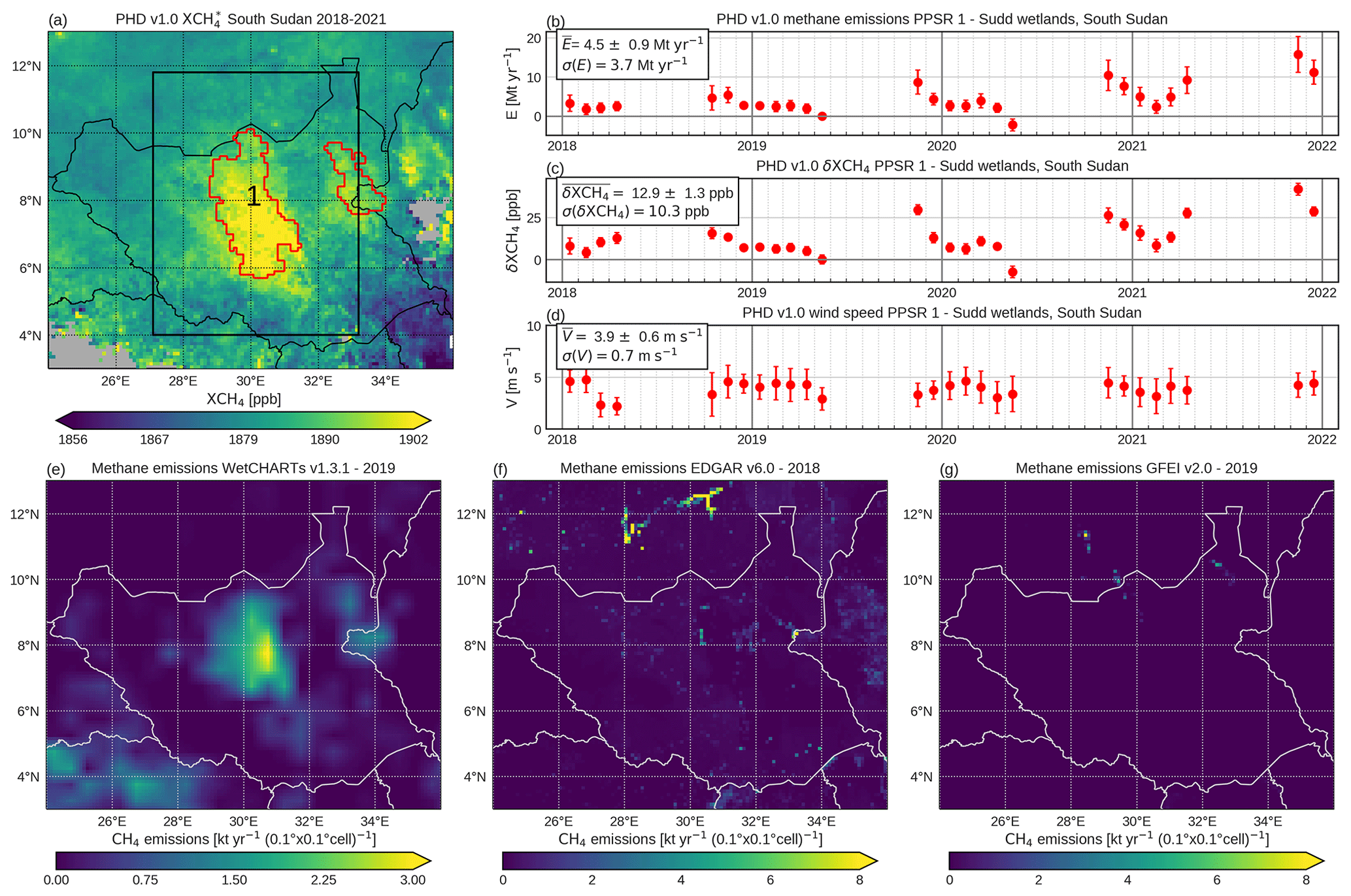
Figure 12 Results for the South Sudan region. (a) The 2018–2021 XCH₄ with the detected PPSR masks outlined in red. The 1 indicates that this region is the PPSR with the highest emission estimate detected by the PHD algorithm for 2018–2021. The black-outlined area defines the surrounding region used to calculate the XCH₄ enhancements δXCH₄. (b) Time series (2018–2021) of the emission estimates, E; (c) XCH₄ enhancements, δXCH₄; and (d) mean wind speed, V. (e) Methane emissions from WetCHARTs v1.3.1 for 2019, (f) from EDGAR v6.0 for 2018 and (g) from GFEI v2.0 for 2019. The emission estimate of the PPSR for 2018–2021 is $\mathrm{4.5}\pm \mathrm{0.9}\mathrm{Mt}{\mathrm{yr}}^{-\mathrm{1}}$, and the corresponding emissions of the databases in this PPSR are 0.88 Mt yr⁻¹ for WetCHARTs, 0.17 Mt yr⁻¹ for EDGAR and 0.01 Mt yr⁻¹ for GFEI.

Pandey et al. (2021) estimated the methane emissions of the entire wetland region in South Sudan, including the Sudd and other wetlands, to be $\mathrm{8.0}\pm \mathrm{3.2}\mathrm{Mt}{\mathrm{yr}}^{-\mathrm{1}}$ for 2018–2019. In a study from Lunt et al. (2019), emissions of the Sudd region were estimated using GOSAT XCH₄ data, resulting in 5.2–6.9 Mt yr⁻¹ for 2016. Our estimate is lower compared to the two results, which can be explained by the smaller source region of this study. By combining PPSR 1 with the PPSR that we detected in the east of South Sudan ($\mathrm{0.8}\pm \mathrm{0.4}\mathrm{Mt}{\mathrm{yr}}^{-\mathrm{1}}$ for 2018–2021), we get a total emission estimate of $\mathrm{5.3}\pm \mathrm{1.3}\mathrm{Mt}{\mathrm{yr}}^{-\mathrm{1}}$, which is in agreement within the uncertainties of the emissions calculated in Pandey et al. (2021) and Lunt et al. (2019).

The emissions from the databases WetCHARTs v1.3.1, EDGAR v6.0 and GFEI v2.0 for the South Sudan region are shown in Fig. 12e–g. We compute the emissions of the databases in a PPSR by adding all emissions within the extended mask of the PPSR (see Sect. 3.6), which include the directly adjacent outer grid cells of the PPSR, to consider possible source location variations in the databases. WetCHARTs emissions for 2019 in PPSR 1 are 0.88 Mt yr⁻¹. EDGAR emissions for 2018 for PPSR 1, which are mostly from the agriculture sector, combine to 0.17 Mt yr⁻¹ and the emissions from GFEI for 2019 are 0.01 Mt yr⁻¹. It can be seen that the emissions from the databases show a large difference from the emission estimates of this study and from those of Pandey et al. (2021) and Lunt et al. (2019).

4.2.2 Turkmenistan – west coast

The PPSR with the second-highest emission estimate for 2018–2021, called PPSR 2, is detected on the west coast of Turkmenistan, in the Balkan province that borders the Caspian Sea. The dominant source type is determined as oil and gas. The west coast of Turkmenistan is a methane source region with oil and gas infrastructure over almost the entire coastal belt, including oil and gas power plants, compressor stations, and pipelines (Irakulis-Loitxate et al., 2022). An overview of the results for PPSR 2, as well as the mask that defines the PPSR, can be seen in Fig. 13. The mean emission estimate for 2018–2021 is 3.5 Mt yr⁻¹ with an uncertainty of 0.9 Mt yr⁻¹ and a standard deviation of 0.6 Mt yr⁻¹. All months except January and February 2018 contribute to the emission estimate. The mean of the δXCH₄ for the time period is 17.5±1.4 ppb and the mean wind speed $\mathrm{4.3}\pm \mathrm{1.0}\mathrm{m}{\mathrm{s}}^{-\mathrm{1}}$, where ± indicates the corresponding uncertainties.

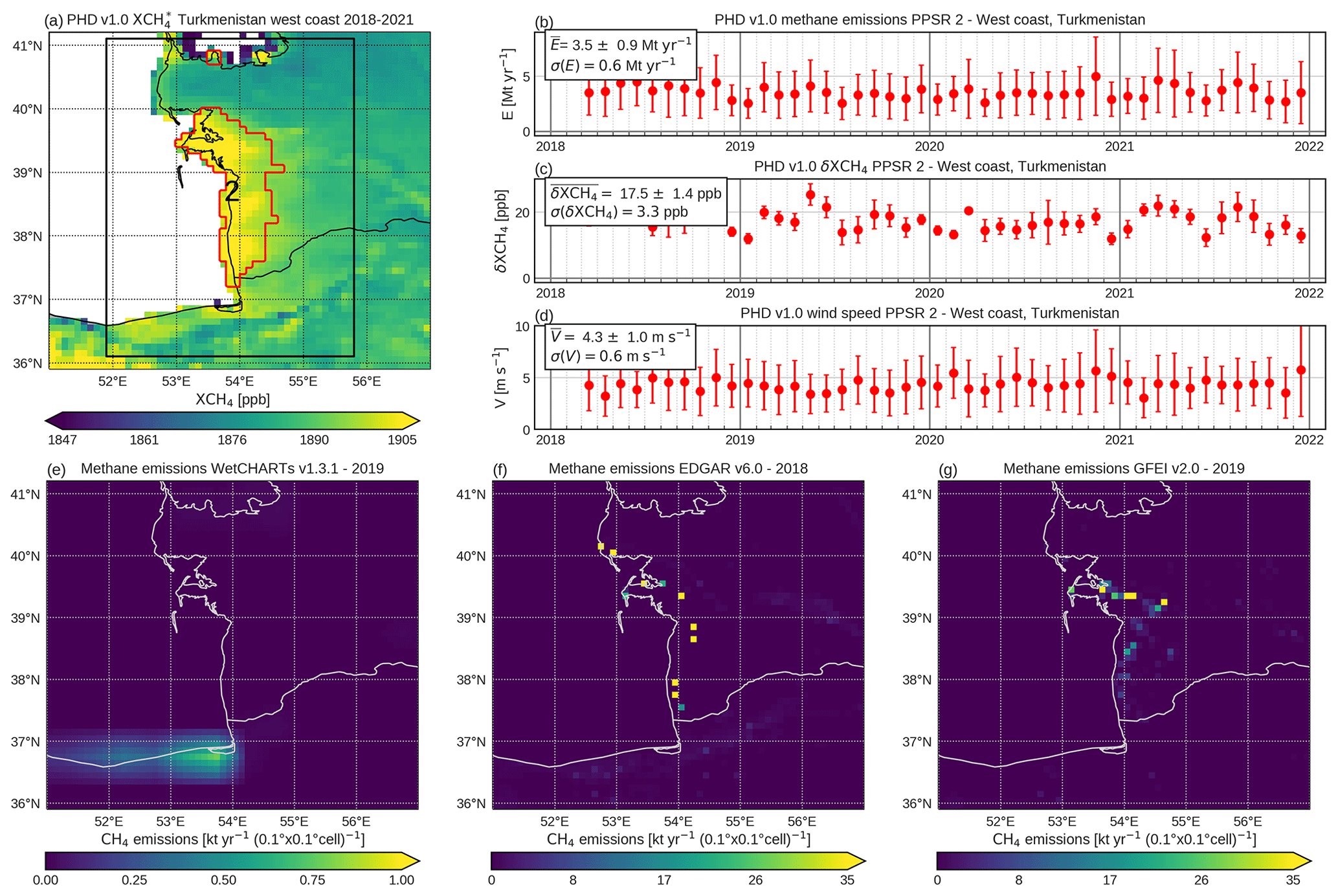
Figure 13 As Fig. 12 but for the west coast of Turkmenistan, where the PPSR with the second-highest emission estimate of $\mathrm{3.5}\pm \mathrm{0.9}\mathrm{Mt}{\mathrm{yr}}^{-\mathrm{1}}$ for 2018–2021 is detected. The corresponding emissions from the databases in PPSR 2 are 0.0 Mt yr⁻¹ for WetCHARTs, 0.64 Mt yr⁻¹ for EDGAR and 0.62 Mt yr⁻¹ for GFEI.

Methane emissions on the west coast of Turkmenistan have been detected in recent studies (He et al., 2024; Irakulis-Loitxate et al., 2022; Barré et al., 2021; Schuit et al., 2023; Varon et al., 2019). In Irakulis-Loitxate et al. (2022), areas on the west coast were identified as hotspot regions using TROPOMI, where hyperspectral (ZY1 and PRISMA) and multispectral (Sentinel-2) satellites detected several localized emission events in the range of kilotons per year from January 2017 to November 2020. In Varon et al. (2019), a methane source was detected at a compressor station in Korpezhe, in the middle of the west coast of Turkmenistan. Using TROPOMI data, the total emissions within a 12×12 km² region around this source were calculated to be 0.45 Mt yr⁻¹ (0.19–0.75) for December 2017 to January 2019. The emissions calculated in these studies refer to individual events or to smaller regions of the west coast and therefore cannot be directly used for comparison with the emission estimates calculated in this study but provide an overview of the magnitude of the emissions.

The spatial distribution of methane emissions from EDGAR v6.0 for 2018 and GFEI v2.0 for 2019 for the region considered are shown in Fig. 13e–g. The emissions from EDGAR of 0.64 Mt yr⁻¹ and GFEI of 0.62 Mt yr⁻¹ for the entirety of PPSR 3 are significantly lower than our estimate of $\mathrm{3.5}\pm \mathrm{1.8}\mathrm{Mt}{\mathrm{yr}}^{-\mathrm{1}}$. Several studies suggested that the inventories may underestimate Turkmenistan's emissions (Lauvaux et al., 2022; Buchwitz et al., 2017; Shen et al., 2023). For example, Shen et al. (2023) calculated emissions of $\mathrm{3.6}\pm \mathrm{1.3}\mathrm{Mt}{\mathrm{yr}}^{-\mathrm{1}}$ related to oil and gas in Turkmenistan using TROPOMI, which are higher than the emissions reported by GFEI of 1.5 Mt yr⁻¹. If we add the mean emission estimates of all oil- and gas-related PPSRs in Turkmenistan, we get a total emission estimate of $\mathrm{5.0}\pm \mathrm{1.4}\mathrm{Mt}{\mathrm{yr}}^{-\mathrm{1}}$, which is in agreement within the uncertainties in Shen et al. (2023).

4.2.3 Argentina – Iberá Wetland

The PPSR with the third-highest emission estimate for 2018–2021, called PPSR 3, is detected in the region of the border between northeastern Argentina and southern Paraguay and is assigned to the wetland type. PPSR 3 is located in the northern part of the Paraná region, a well-known methane source region, which extends from the Iberá Wetland in the north, the second-largest wetland in the world, to the area where the Paraná River flows into the Atlantic Ocean (Parker et al., 2018). In Fig. 14 we show an overview of the results of PPSR 3. The mean emission estimate for 2018–2021 is $\mathrm{3.3}\pm \mathrm{1.1}\mathrm{Mt}{\mathrm{yr}}^{-\mathrm{1}}$ with a standard deviation of 1.3 Mt yr⁻¹, and the mean of the corresponding δXCH₄ is 8.9±1.9 ppb. The emissions show a seasonal cycle, which also can be seen in the δXCH₄ time series and which is in good agreement with the wet season (Ortega et al., 2022; Parker et al., 2018). Furthermore, the emission estimates show a slight decrease from 2020 onward, which agrees with the results in Lin et al. (2023), where methane emission changes between 2019 and 2021 are analyzed, including the emission changes in the Paraná region.

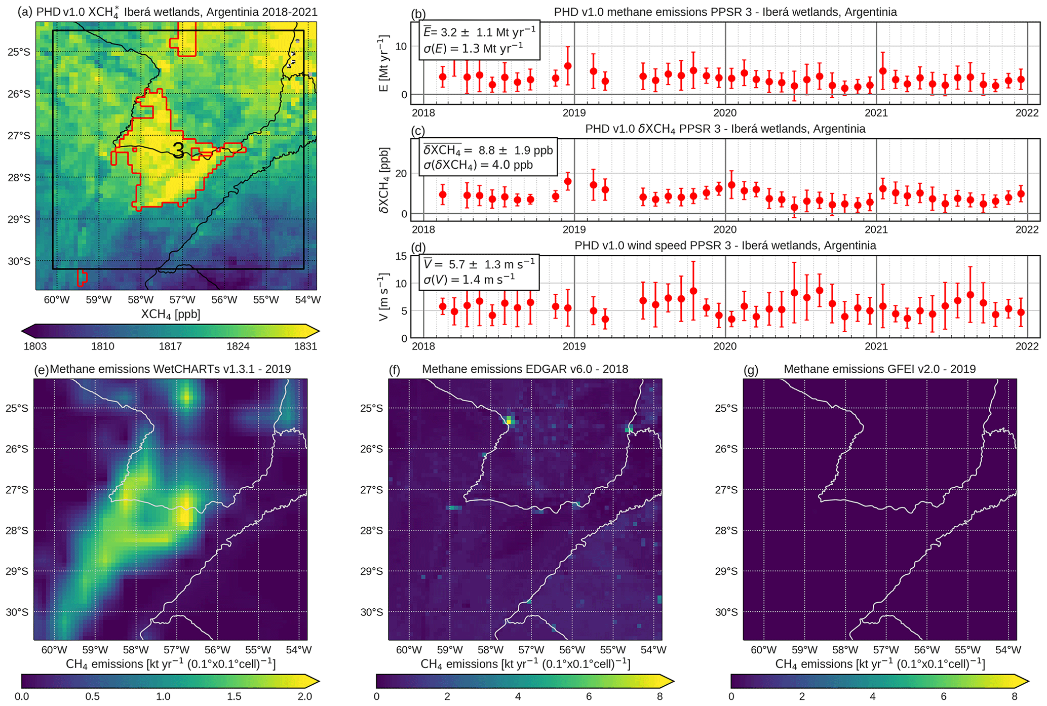
Figure 14 As Fig. 12 but for the Iberá Wetlands in Argentina, where the PPSR with the third-highest emission estimate of $\mathrm{3.3}\pm \mathrm{1.0}\mathrm{Mt}{\mathrm{yr}}^{-\mathrm{1}}$ for 2018–2021 is detected. The corresponding emissions from the databases in PPSR 3 are 0.64 Mt yr⁻¹ for WetCHARTs, 0.18 Mt yr⁻¹ for EDGAR and 0.0 Mt yr⁻¹ for GFEI.

WetCHARTs v1.3.1 shows enhanced methane emissions for the entire Paraná region, especially for Iberá Wetland, whereas the anthropogenic databases indicate only low emissions (Fig. 14e–g). WetCHARTs emissions for PPSR 3 are 0.64 Mt yr⁻¹, which is below our emission estimate. Although the Paraná region is a known methane source region, until now, no studies have calculated the absolute values of the emissions from this region that we can use to further assess our emission estimates. For example, in Parker et al. (2018), XCH₄ retrieved from GOSAT observations is used to analyze how well the methane interannual variability is described by model simulations for several regions, including the Paraná, without reporting explicit emission estimates.

4.2.4 China – Liaoning

The PPSR with the fourth-highest emission estimate for 2018–2021, called PPSR 4, is detected in Liaoning province in northeast China and is assigned to type other anthropogenic. Liaoning is known for its high agricultural production (e.g., rice cultivation and livestock) as well as for its large heavy industry, including strong coal mining activities. The results of PPSR 4 are shown in Fig. 15. The PPSR mask covers the region of Liaoning province where most of the rice production takes place and where a majority of the coal mines are located (Ma et al., 2021; Sheng et al., 2019). The mean emission estimate is 2.9 Mt yr⁻¹ with an uncertainty of 0.9 Mt yr⁻¹ and a standard deviation of 1.0 Mt yr⁻¹. The δXCH₄ has a mean of 8.1±1.6 ppb and shows strong variability over the years with a standard deviation of 2.5 ppb, with the minimum usually in spring. In all months from 2018 to 2021, the PPSR as well as the background region are filled with sufficient XCH₄ values to calculate the δXCH₄ and the emission estimates.

So far, there are only a few studies that have analyzed or identified methane emissions in the region considered. For example, two plumes were detected in 2021 by Schuit et al. (2023), which are located in the PPSR, with one plume assigned to the coal source type and one plume assigned to the landfill type. In Sheng et al. (2019), coal-related emissions in 2011 for China, including the Liaoning region, were estimated by analyzing reports from over 10 000 coal mines in China. For Liaoning, the coal-related emissions were calculated to be 1.04 Mt yr⁻¹. The different time periods, as well as the larger region considered in Sheng et al. (2019), make it difficult to compare the results with the results of this study. In Foy et al. (2023) emissions of urban areas were estimated using TROPOMI data and compared with EDGAR, including the Shenyang region in Liaoning, where the emissions were estimated at 1.6 Mt yr⁻¹. If we take into account the fact that the Shenyang region is smaller than PPSR 5 and thus some emissions from the surrounding area are not included in the estimate, our result is in good agreement with that of Foy et al. (2023).

It can be seen from Fig. 15e–g that anthropogenic emissions are the dominant source type in this region. Emissions from EDGAR for PPSR 4 are 1.3 Mt in total for 2018, with large emissions seen in Shenyang, the capital of Liaoning. Of the 1.3 Mt, 52 % are from the category of other anthropogenic sources, which is composed of emissions from several sectors, such as rice cultivation or landfills. The remaining emissions from EDGAR are related to the fossil fuel sector, mainly to coal production, which is in the range of the fossil-fuel-related emissions from GFEI in 2019 for the PPSR of 0.49 Mt yr⁻¹. The emissions from the databases are significantly lower than the emissions calculated in this study of $\mathrm{2.9}\pm \mathrm{0.9}\mathrm{Mt}{\mathrm{yr}}^{-\mathrm{1}}$, which is also reported in Foy et al. (2023) for their emission estimate of the Shenyang region.

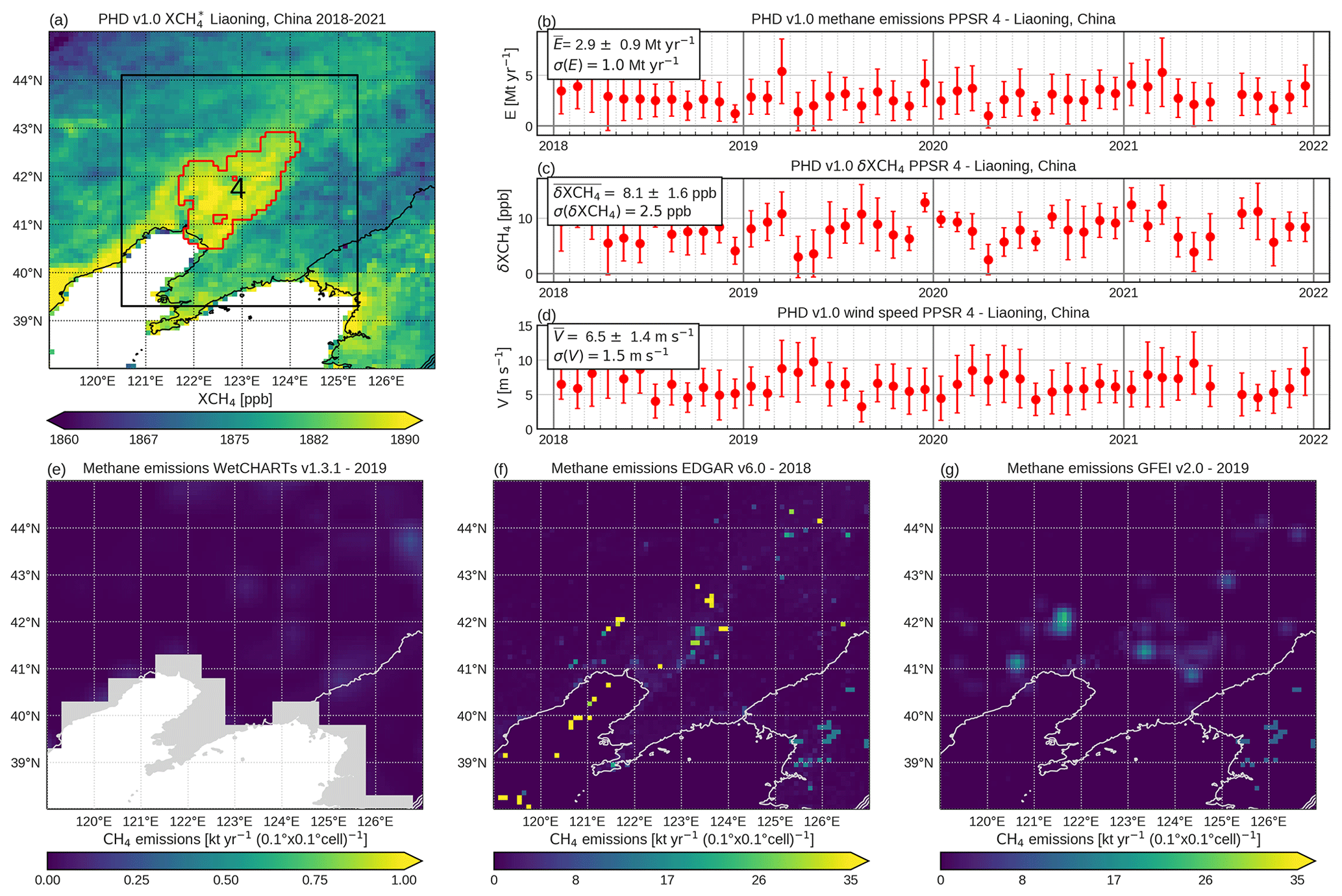
Figure 15 As Fig. 12 but for the Liaoning region in China, where the PPSR with the fourth-highest emission estimate of $\mathrm{2.9}\pm \mathrm{0.9}\mathrm{Mt}{\mathrm{yr}}^{-\mathrm{1}}$ for 2018–2021 is detected. The corresponding emissions from the databases in PPSR 4 are 0.0 Mt yr⁻¹ for WetCHARTs, 1.3 Mt yr⁻¹ for EDGAR and 0.49 Mt yr⁻¹ for GFEI.

4.2.5 China – Shanxi

The PPSRs with the fifth-, sixth- and seventh-highest emission estimates for 2018–2021, called PPSRs 5, 6 and 7, are detected in the Shanxi province in north China. The Shanxi province is a known methane source region with emissions resulting primarily from heavy coal mining activity (Peng et al., 2023). This corresponds to the dominant source type of the three PPSRs that was determined, which is coal. An overview of the results of the individual PPSRs is shown in Fig. 16. Figure 16a shows the 2018–2021 XCH₄ for Shanxi and the surroundings, including the detected PPSR masks, as well as the corresponding background regions for PPSRs 5, 6 and 7. It can be seen that the XCH₄ in the PPSRs is enhanced compared to the XCH₄ in the surrounding regions. The time series of the δXCH₄ for the PPSRs are shown in Fig. 16c. PPSR 5 has a mean δXCH₄ for 2018–2021 of 25.1±2.5 ppb, PPSR 6 of 20.6±1.8 ppb and PPSR 7 of 22.3±2.2 ppb, which are the highest mean δXCH₄ values of all detected PPSRs. The δXCH₄ shows a strong variability in all three PPSRs with standard deviations of 10.4 ppb for PPSR 5, 6.5 ppb for PPSR 6 and 4.8 ppb for PPSR 7. This variability can also be seen in the emission estimates of the PPSRs shown in Fig. 16b. The mean emission estimates are $\mathrm{2.6}\pm \mathrm{0.8}\mathrm{Mt}{\mathrm{yr}}^{-\mathrm{1}}$ for PPSR 5, $\mathrm{2.6}\pm \mathrm{0.7}\mathrm{Mt}{\mathrm{yr}}^{-\mathrm{1}}$ for PPSR 6 and $\mathrm{2.4}\pm \mathrm{0.7}\mathrm{Mt}{\mathrm{yr}}^{-\mathrm{1}}$ for PPSR 7, and in all three PPSRs almost all months contribute to the corresponding mean emission estimate.

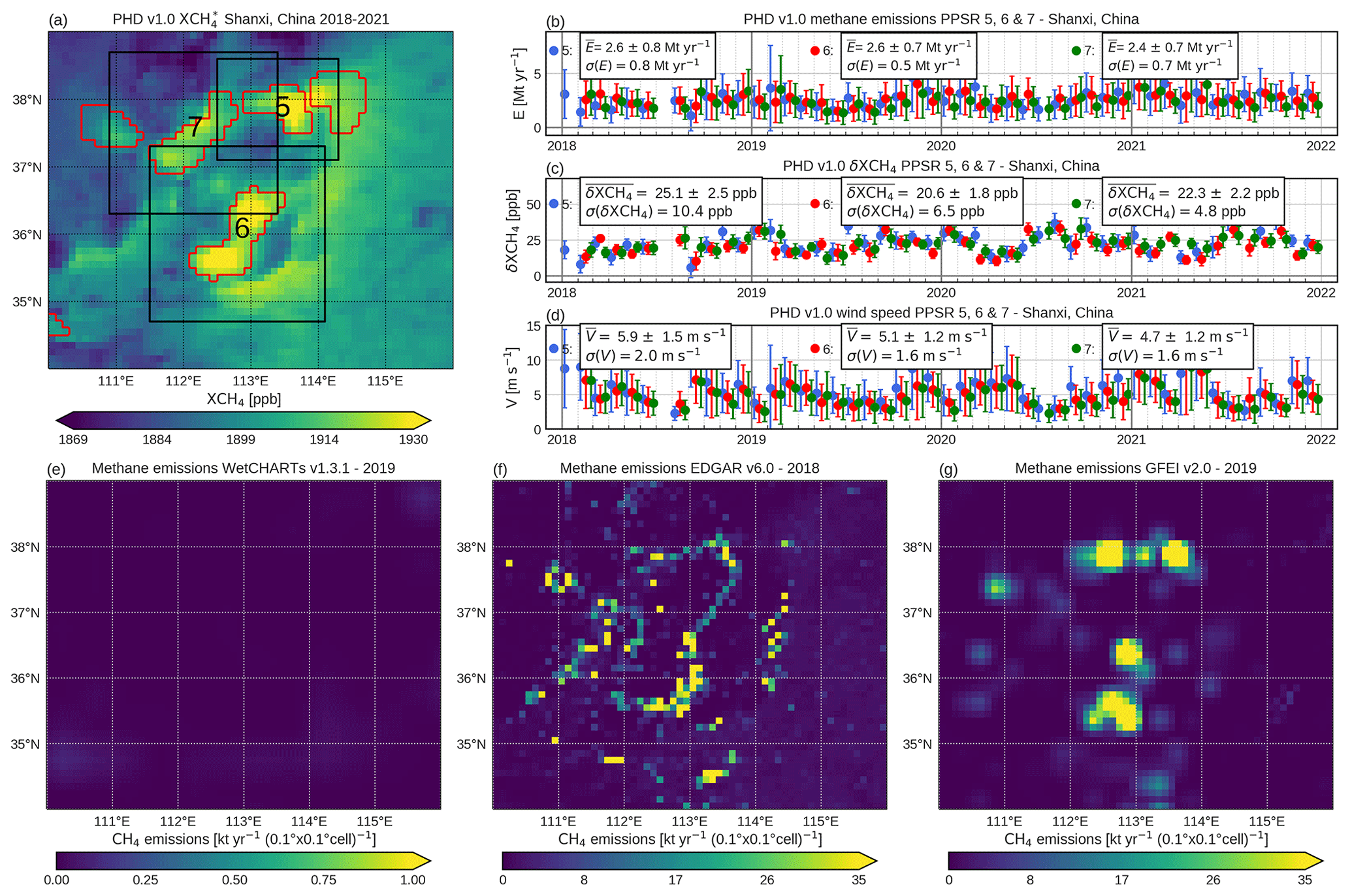
Figure 16 As Fig. 12 but for the Shanxi region in China, where the PPSRs with the fifth- ($\mathrm{2.6}\pm \mathrm{0.8}\mathrm{Mt}{\mathrm{yr}}^{-\mathrm{1}}$), sixth- ($\mathrm{2.6}\pm \mathrm{0.7}\mathrm{Mt}{\mathrm{yr}}^{-\mathrm{1}}$) and seventh-highest ($\mathrm{2.4}\pm \mathrm{0.7}\mathrm{Mt}{\mathrm{yr}}^{-\mathrm{1}}$) emission estimates for 2018–2021 are detected. The corresponding emissions of the databases in PPSRs 5, 6 and 7 are 0 Mt yr⁻¹ for WetCHARTs; 1.2 Mt yr⁻¹ (PPSR 5), 2.8 Mt yr⁻¹ (PPSr 6), and 1.2 Mt yr⁻¹ (PPSR 7) for EDGAR; and 1.5 Mt yr⁻¹ (PPSR 5), 2.5 Mt yr⁻¹ (PPSR 6), and 1.9 Mt yr⁻¹ (PPSR 7) for GFEI.

Methane emissions in Shanxi have already been detected in several studies. The main focus was on the detection of individual plumes, which were identified, for example, by analyzing TROPOMI data as in Schuit et al. (2023) and Lauvaux et al. (2022); by data from the Worldview 3 satellite as in Sánchez-García et al. (2022); or by data from the PRISMA satellite mission as in Guanter et al. (2021). The detected transient plumes in these studies are not suitable for comparison with our emission estimates, which were evaluated for persistent hotspot regions for several years. But this is the case for the study by Peng et al. (2023) in which the coal-related methane emissions for the entire Shanxi region for the years 2019 and 2020 were calculated by inversion of TROPOMI data. Peng et al. (2023) estimated emissions for 2019 of $\mathrm{8.5}\pm \mathrm{0.6}\mathrm{Mt}{\mathrm{yr}}^{-\mathrm{1}}$ and for 2020 of $\mathrm{8.6}\pm \mathrm{0.6}\mathrm{Mt}{\mathrm{yr}}^{-\mathrm{1}}$. To compare, we computed the sum of the emissions of all the detected PPSRs in Shanxi (PPSRs 5, 6, 7 and one other PPSR with a mean emission estimate of $\mathrm{1.1}\pm \mathrm{0.3}\mathrm{Mt}{\mathrm{yr}}^{-\mathrm{1}}$ for 2018–2021; see Fig. 16a) and obtained an emission estimate of $\mathrm{8.8}\pm \mathrm{2.4}\mathrm{Mt}{\mathrm{yr}}^{-\mathrm{1}}$ for the period 2018–2021, which is in agreement within the uncertainties in the results from Peng et al. (2023). Moreover, by considering the emission estimates for 2019 and 2020, we obtained $\mathrm{8.5}\pm \mathrm{2.1}\mathrm{Mt}{\mathrm{yr}}^{-\mathrm{1}}$ for 2019 and $\mathrm{8.7}\pm \mathrm{1.8}\mathrm{Mt}{\mathrm{yr}}^{-\mathrm{1}}$ for 2020 for the combined PPSRs in Shanxi. In Peng et al. (2023), the entire Shanxi region is considered, while we only focused on parts of the region. However, if we assume that our identified hotspots in the Shanxi region contain the majority of methane emissions, the comparison of the two results is reasonable.

Figure 16e–g shows the methane emissions of WetCHARTs v1.3.1, EDGAR v6.0 and GFEI v2.0 for Shanxi and the surrounding area. It can be seen that the region is dominated by anthropogenic emissions. The emissions for 2018 from EDGAR are mainly related to coal production and are 1.2 Mt yr⁻¹ for PPSR 5, 2.8 Mt yr⁻¹ for PPSR 6 and 1.2 Mt yr⁻¹ for PPSR 7 in the corresponding extended PPSR masks. In total, the EDGAR emissions of all PPSRs in Shanxi combine to 5.2 Mt yr⁻¹, which is below our emission estimate of $\mathrm{8.8}\pm \mathrm{2.4}\mathrm{Mt}{\mathrm{yr}}^{-\mathrm{1}}$ for 2018–2021. The emissions from GFEI for 2019 are mostly related to the coal sector and are concentrated in a few hotspots, which correlate with the locations of the detected PPSRs. For PPSR 5, the GFEI emissions are 1.5 Mt yr⁻¹, 2.5 Mt yr⁻¹ for PPSR 6 and 1.9 Mt yr⁻¹ for PPSR 7. The total GFEI emissions of the PPSRs considered are 5.9 Mt yr⁻¹, which is slightly higher than the emissions reported by EDGAR but lower than the emission estimates of this study and the study by Peng et al. (2023).

4.2.6 Bangladesh – Dhaka and surrounding area

The PPSR with the eighth-highest emission estimate for 2018–2021, called PPSR 8, is detected in a region encompassing Dhaka, the capital of Bangladesh, which is one of the most populated cities in the world. The dominant source type is determined to be other anthropogenic sources. Dhaka and the surrounding area are a known methane source region with the main sources being agricultural production (rice, livestock) and waste management (wastewater, landfills) but also with contributions from wetlands (Foy et al., 2023; Toha and Rahman, 2023). The results for PPSR 8 are shown in Fig. 17. The 2018–2021 XCH₄ shows a strong enhancement in the PPSR, especially in and around Dhaka, compared to the XCH₄ of the surrounding area (see Fig. 17a). The δXCH₄ values for 2018–2021 are shown in Fig. 17c, averaging to a mean of 21.4±2.0 ppb, which is in the range of the enhancements of the PPSRs in the Shanxi region. For the years considered, no XCH₄ is present for the period from March/April to October/November due to the monsoon season and the resulting frequent high cloud coverage. Figure 17b shows the emission estimates for 2018–2021 with a mean of $\mathrm{2.4}\pm \mathrm{0.5}\mathrm{Mt}{\mathrm{yr}}^{-\mathrm{1}}$ and increasing values from October/November until April/May of the following year. This period is also one of two phases in which the rice is cultivated in Bangladesh. The first phase is in summer, which starts around June and ends in October with the harvest. The second phase is during the winter from November to April, when the fields are artificially irrigated (Rahman et al., 2023).

Methane emissions in Dhaka have already been detected and quantified in several studies (Foy et al., 2023; Schuit et al., 2023). Schuit et al. (2023) used TROPOMI data to detect plumes worldwide and detected as many plumes as in any other urban area in Dhaka. The emissions from Dhaka are calculated in Foy et al. (2023) using TROPOMI data and a two-dimensional plume model, resulting in emissions of 1.3 Mt yr⁻¹, which is lower than our estimate of $\mathrm{2.4}\pm \mathrm{0.5}\mathrm{Mt}{\mathrm{yr}}^{-\mathrm{1}}$. It must be taken into account that our region is larger than that of Foy et al. (2023) and can therefore include emissions from other cities in the surrounding area, as well as wetland emissions from the Ganges delta.

Figure 17e–g shows the emissions from WetCHARTs v1.3.1, Edgar v6.0 and GFEI v2.0 for the Dhaka region. For WetCHARTs, the emissions in the PPSR amount to 0.13 Mt for 2019; for EDGAR, 0.92 Mt for 2018; and for GFEI, 0.02 Mt for 2019. The emissions from EDGAR are mainly from the agricultural sector, with 0.38 Mt yr⁻¹ from rice production and 0.15 Mt yr⁻¹ from enteric fermentation, and are lower than our calculated emission estimate. In Foy et al. (2023), the calculated emissions were also higher compared to EDGAR. They concluded that part of the difference between EDGAR and their emission estimate is due to the fact that untreated wastewater is not taken into account, which can be a major factor, especially in very densely populated cities such as Dhaka.

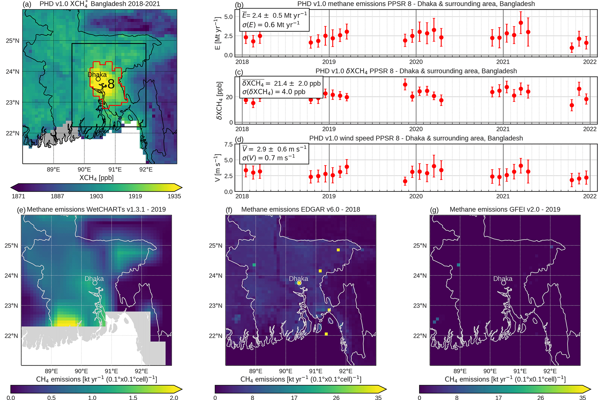
Figure 17 As Fig. 12 but for the region in and around Dhaka in Bangladesh, where the PPSR with the eighth-highest emission estimate of $\mathrm{2.4}\pm \mathrm{0.5}\mathrm{Mt}{\mathrm{yr}}^{-\mathrm{1}}$ for 2018–2021 is detected. The corresponding emissions from the databases in PPSR 8 are 0.13 Mt yr⁻¹ for WetCHARTs, 0.92 Mt yr⁻¹ for EDGAR and 0.02 Mt yr⁻¹ for GFEI.

4.2.7 Russia – Kuznetsk Basin

The PPSR with the ninth-highest emission estimate for 2018–2021, called PPSR 9, is detected in the Kuznetsk Basin (also called Kuzbass) in southwestern Siberia, Russia. Its dominant source type is determined to be coal, which coincides with the fact that Kuzbass is one of the largest coal production areas worldwide (Labzovskii et al., 2022). Figure 18 shows an overview of the results for PPSR 9. In the 2018–2021 XCH₄ map shown in Fig. 18a, a strong enhancement can be seen in the entire PPSR mask compared to the XCH₄ of the surrounding area. To quantify the XCH₄ enhancements within the PPSR, we computed the monthly δXCH₄ for the time period 2018–2021, which is on average 17.3±0.6 ppb with a standard deviation of 6.6 ppb. The mean emission estimate is 2.4 Mt yr⁻¹ with an uncertainty of 0.5 Mt yr⁻¹, which is computed from emission estimates of 30 months (Fig. 18b).

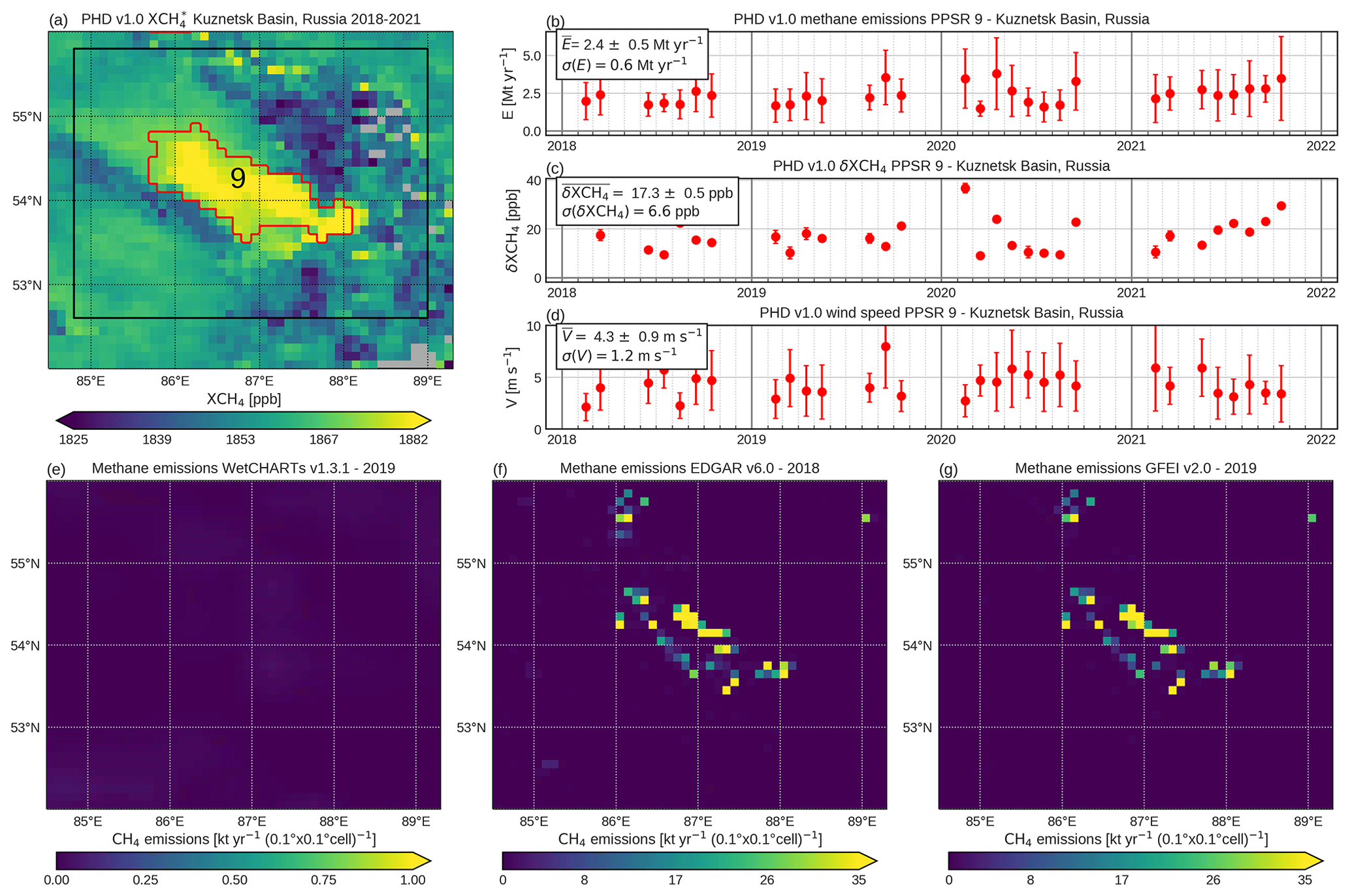
Figure 18 As Fig. 12 but for the Kuznetsk Basin in Russia, where the PPSR with the ninth-highest emission estimate of $\mathrm{2.4}\pm \mathrm{0.5}\mathrm{Mt}{\mathrm{yr}}^{-\mathrm{1}}$ for 2018–2021 is detected. The corresponding emissions from the databases in PPSR 9 are 0.0 Mt yr⁻¹ for WetCHARTs, 1.6 Mt yr⁻¹ for EDGAR and 1.4 Mt yr⁻¹ for GFEI.

Even though the Kuzbass is one of the largest coal production areas worldwide, there is still a need for studies reporting methane emissions from this region. In Schuit et al. (2023), methane plumes are detected in this region but not discussed in more detail. Due to the limited number of studies, we only compare our emission estimate with the emissions from the databases, which are shown in Fig. 18e–g for the region considered. It can be seen that the emissions from the databases are dominated by anthropogenic activity and that the emission hotspots reported by EDGAR and GFEI show a high spatial correlation. EDGAR reports emissions of 1.6 Mt for 2018 and GFEI of 1.4 Mt for 2019, in which the emissions from both databases are mainly related to the coal sector. Compared to the emission estimate of this study, the emissions from EDGAR and GFEI are lower but still within the uncertainty range.

4.2.8 USA – Permian Basin

The PPSR with the 10th-highest emission estimate for 2018–2021, called PPSR 10, is detected in the Permian Basin in the USA and is assigned to the source type oil and gas. The Permian Basin is the most prolific oil field in the USA and is also a high-producing natural gas region, which is located in western Texas and eastern New Mexico. The Permian Basin consists of several sub-basins, including the Delaware Basin in the west and the Midland Basin in the east, where mostly non-conventional exploitation techniques, such as hydraulic fracturing, are used. An overview of the results for PPSR 10 are shown in Fig. 19. It can be seen that we detect two regions in the Permian Basin: PPSR 10 in the Delaware Basin and a PPSR in the Midland Basin, which shows the 13th-strongest emission estimate. Since the literature often refers to the emissions of the entire Permian Basin, we analyze these two PPSRs together. The monthly emission estimates for 2018–2021 are shown in Fig. 19b. The mean emission estimate for PPSR 10 is $\mathrm{2.2}\pm \mathrm{0.6}\mathrm{Mt}{\mathrm{yr}}^{-\mathrm{1}}$ and $\mathrm{2.0}\pm \mathrm{0.5}\mathrm{Mt}{\mathrm{yr}}^{-\mathrm{1}}$ for PPSR 13, which leads to a combined mean emission estimate of $\mathrm{4.1}\pm \mathrm{1.1}\mathrm{Mt}{\mathrm{yr}}^{-\mathrm{1}}$ for 2018–2021 (taking into account the second decimal place). The δXCH₄ time series for 2018–2021 for PPSRs 10 and 13 can be seen in Fig. 19c. The mean δXCH₄ enhancement for PPSR 10 is 7.5±0.6 ppb with a standard deviation of 3.3 ppb and 7.2±0.6 ppb for PPSR 13 with a standard deviation of 1.7 ppb.

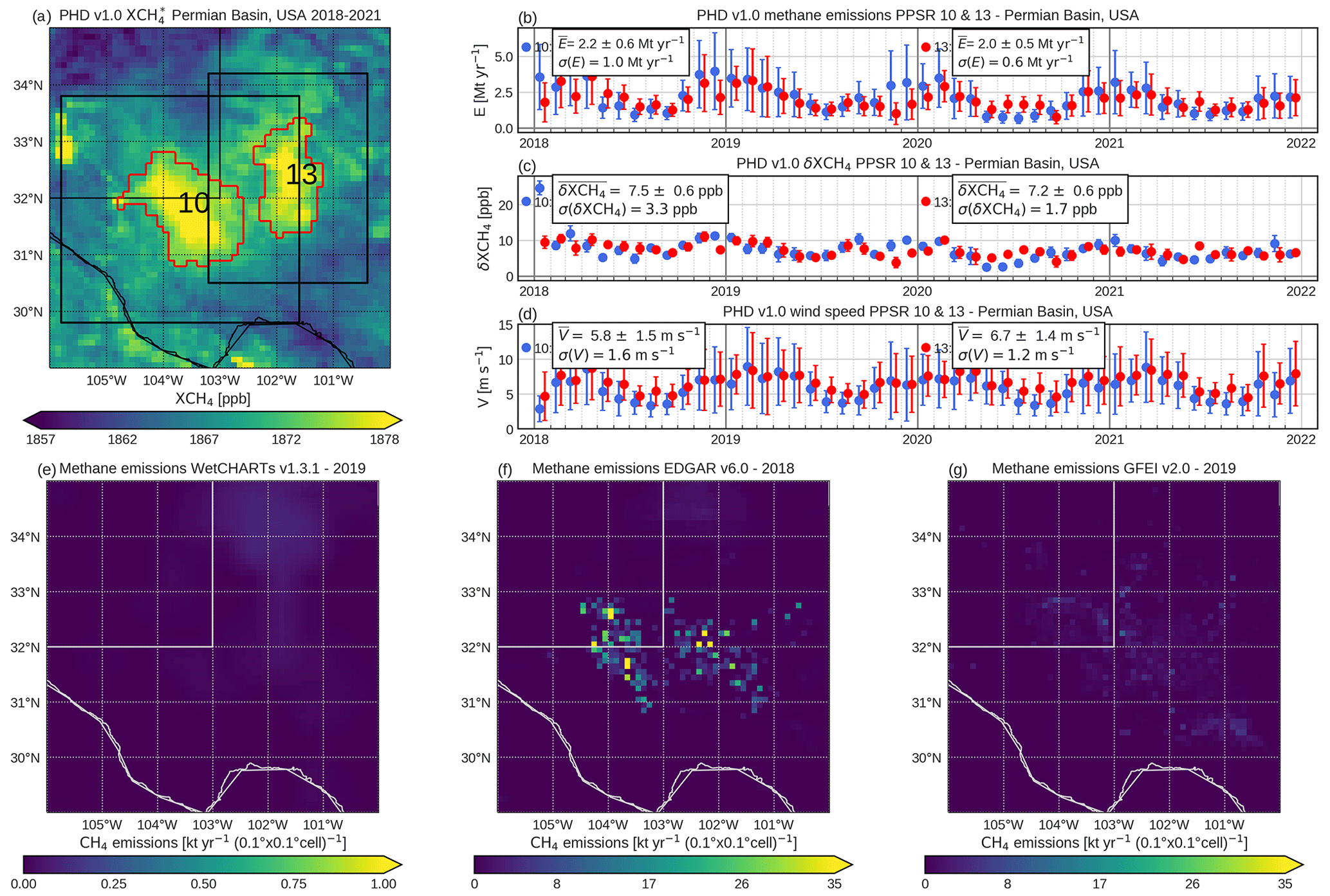
Figure 19 As Fig. 12 but for the Permian Basin in the USA, where the PPSRs with the 10th- and 13th-highest emission estimates for 2018–2021 are detected. The corresponding emissions from the databases in PPSRs 10 (blue, $\mathrm{2.2}\pm \mathrm{0.6}\mathrm{Mt}{\mathrm{yr}}^{-\mathrm{1}}$) and 13 (red, $\mathrm{2.0}\pm \mathrm{0.5}\mathrm{Mt}{\mathrm{yr}}^{-\mathrm{1}}$) are 0.0 Mt yr⁻¹ for WetCHARTs, 1.2 Mt yr⁻¹ (PPSR 10) and 0.59 Mt yr⁻¹ (PPSR 13) for EDGAR, and 0.21 Mt yr⁻¹ (PPSR 10) and 0.14 Mt yr⁻¹ (PPSR 13) for GFEI.

Methane emissions from the Permian basins have already been quantified in several studies (Schneising et al., 2020; Shen et al., 2022; Varon et al., 2023; Veefkind et al., 2023; Zhang et al., 2020). In the studies by Schneising et al. (2020) and Veefkind et al. (2023), emissions were calculated based on the TROPOMI/WFMD XCH₄ data product. Schneising et al. (2020) used a Gaussian integral method and estimated emissions of $\mathrm{3.2}\pm \mathrm{1.1}\mathrm{Mt}{\mathrm{yr}}^{-\mathrm{1}}$ for the period 2018-2019, whereas Veefkind et al. (2023) calculated emissions of $\mathrm{3.0}\pm \mathrm{0.7}\mathrm{Mt}{\mathrm{yr}}^{-\mathrm{1}}$ for 2019 using a divergence method. The emissions reported in the studies by Zhang et al. (2020), Shen et al. (2022) and Varon et al. (2023) are based on the operational TROPOMI data product and different inversion frameworks. Zhang et al. (2020) calculated emissions of $\mathrm{2.9}\pm \mathrm{0.5}\mathrm{Mt}{\mathrm{yr}}^{-\mathrm{1}}$ for the period from May 2018 to March 2019, whereas Shen et al. (2022) estimated emissions of $\mathrm{2.9}\pm \mathrm{0.4}\mathrm{Mt}{\mathrm{yr}}^{-\mathrm{1}}$ for the period from May 2018 to February 2020 and of $\mathrm{3.7}\pm \mathrm{0.5}\mathrm{Mt}{\mathrm{yr}}^{-\mathrm{1}}$ for the same period but with an adjusted prior. In Varon et al. (2023), the period from May 2018 to October 2020 is considered and mean emissions of $\mathrm{3.7}\pm \mathrm{0.9}\mathrm{Mt}{\mathrm{yr}}^{-\mathrm{1}}$ are reported, which is higher than the previous emission estimates. The emission estimate of $\mathrm{4.1}\pm \mathrm{1.1}\mathrm{Mt}{\mathrm{yr}}^{-\mathrm{1}}$ for 2018–2021 calculated in this study is slightly higher than the emissions of the other studies presented but agrees within the uncertainties.

The emissions from EDGAR v6.0, GFEI v2.0 and WetCHARTs v1.3 are shown in Fig. 19e–g. For EDGAR, the emissions within the extended PPSR mask (see Sect. 3.6) are 1.2 Mt yr⁻¹ and 0.2 Mt yr⁻¹ for GFEI and relate to the oil and gas sector. The emissions of both databases are significantly lower than the emission estimates of this study and the other studies mentioned above. The emissions of these two databases also differ from one another.

5 Conclusions

We developed an automated algorithm that uses TROPOMI XCH₄ data to identify potential persistent methane source regions (PPSRs), to estimate their emissions and to assign a source type to them. We applied the algorithm to a dataset comprising monthly averaged XCH₄ maps at 0.1°×0.1° spatial resolution from 2018 to 2021, which we generated by gridding the TROPOMI/WFMD v1.8 data product. The detection process involves two key steps: (i) the generation of monthly methane anomaly maps (ΔXCH₄), which indicate how high or low a local XCH₄ value is compared to the median of the surrounding XCH₄ and (ii) the analysis of these anomaly maps. In the latter, we characterized each region by several quantities, such as the number of months in which the region shows enhanced anomalies, to then identify regions with a persistent enhancement by defining threshold values for the corresponding quantities. The algorithm is designed in a way that the thresholds can be adjusted depending on the focus of the source regions to be detected. For the automated emission estimates of the individual PPSRs, we used a fast data-driven mass balance method, which is designed to calculate emission estimates from time-averaged XCH₄ maps. For more precise emission estimates, we recommend conducting more detailed analyses based on daily data. To determine the dominant source types of the PPSRs, we compared the emissions from several databases (WetCHARTs v1.3.1, EDGAR v6.0 and GFEI v2.0) within the PPSR masks.

We detected a total of 217 PPSRs, of which 17 are assigned to the dominant source type coal, 17 are assigned to the type oil and gas, 66 to the source type other anthropogenic sources, 16 to the wetland type and 101 are assigned to the unknown source type. We showed that TROPOMI data can be used to detect a variety of well-known methane source regions such as large oil and gas fields in Turkmenistan and the USA but also small-scale source regions like coal mines in Queensland in Australia. The emission estimates of all detected PPSRs amount to about 150 Mt yr⁻¹, which corresponds to approximately 20 % of the bottom-up emissions reported in Saunois et al. (2020). We found that the majority of emissions (35.4 %) are associated with PPSRs dominated by other anthropogenic sources, followed by PPSRs of unknown type (27.2 %), coal type (13.0 %), oil and gas type (12.5 %) and wetland type (11.9 %). The coal-dominated source regions describe almost half (44.5 %) of global coal emissions of Saunois et al. (2020), while those from oil and gas (22.3 %), as well as other anthropogenic sources (21.8 %), also account for a large share of their sectors' emissions. This demonstrates that a comparatively small number of high-emitting source regions contribute a large proportion to the global methane emissions, underlining the importance of their detection and quantification for improving the understanding of the global methane emissions. The detected wetland regions account for 4.9 % of the total natural emissions reported in Saunois et al. (2020). However, we note that in some known wetland areas, such as Lake Chad or the Inner Niger Delta (Mali), strongly emitting PPSRs were detected but were assigned to other source types due to the comparatively lower emissions in the wetland database. In addition, a more detailed analysis showed that many of the PPSRs with the unknown source type are wetland regions. In total, 46.5 % of the PPSRs show emissions of less than 50 kt yr⁻¹ in the emission databases and were thus labeled as source regions with an unknown source type. The emission estimates of the unknown PPSRs range from 0.12–1.2 Mt yr⁻¹, indicating that in these regions the emission estimates of this study and the emissions in the databases have large differences. Some of the unknown PPSRs have been identified as methane sources in other studies, such as the PPSRs we detected in the Surat Basin in Australia or in the wetland region in Zambia. We found differences between the emissions of the databases and our emission estimates not only for the PPSRs with an unknown source type but also for some of the PPSRs with the 10 highest mean emission estimates for 2018–2021. These regions are located in the Sudd Wetlands in South Sudan; on the west coast of Turkmenistan, which is an area dominated by oil and gas infrastructure; in the Iberá wetland in Argentina; in the Liaoning and Shanxi provinces in China, which are known rice- and coal-production areas; in the city of Dhaka and its surroundings in Bangladesh; in the Kuznetsk Basin in Russia, one of the largest coal production areas in the world; and in the Permian Basin, a large oil and gas field in the United States. For many of these PPSRs, the emission estimates are in agreement within the uncertainties in emission estimates from other studies. In the emission databases, these PPSRs are also shown as methane hotspots, but their emissions are significantly lower compared to our emission estimates. Further studies are needed to analyze the differences between the emissions of the databases and emission estimates in this and other studies in more detail. Furthermore, we cannot exclude the possibility that some of the detected PPSRs may be false positives. To improve the filtering of potential false positives, additional parameters, such as the aerosol optical thickness, could be considered in the analysis. Since the distinction between true- and false-positive detection is not trivial in many cases, it often requires detailed analyses. For example, in Schuit et al. (2023), as well as in Lauvaux et al. (2022), human observers subsequently verify each detected plume. Such an approach was omitted in this work in order to provide a fully automated algorithm.

Each of the detected PPSRs is a potential source region that needs to be examined in more detail, for example using a similar analysis as was conducted for the PPSRs with the 10 highest emission estimates. Furthermore, an additional analysis of the daily data can provide new insights into the characteristics of the regions. This includes the potential to use other methods for the calculation of the emission estimates (e.g., a Gaussian integral method) or to perform detailed analyses to classify the PPSRs in terms of false-positive detection. For example, preliminary analyses of PPSRs 165 and 217 in Germany have shown that their emission estimates of $\mathrm{0.29}\pm \mathrm{0.07}\mathrm{Mt}{\mathrm{yr}}^{-\mathrm{1}}$ (PPSR 165) and $\mathrm{0.12}\pm \mathrm{0.03}\mathrm{Mt}{\mathrm{yr}}^{-\mathrm{1}}$ (PPSR 217) are likely too high because of potential retrieval biases and/or accumulation of methane in the coal pits, which means that the assumptions of the method for calculating emissions do not match the characteristics of these regions. Methane retrievals directly over the coal pits are challenging due to complex and evolving topography and reflectivity variations.

Moreover, a more detailed comparison between the regions detected in this study and the results of the studies from Schuit et al. (2023) and Lauvaux et al. (2022), in which methane hotspots were also detected using TROPOMI data, is of interest. The studies differ in their focus on the type of hotspot to be detected. In Schuit et al. (2023) and Lauvaux et al. (2022) the focus is on plumes originating from point sources, including short-term emissions such as gas well blowouts, while in this study persistent source regions are detected, which also include larger-scale source regions in addition to point sources. Despite these differences, a detailed comparison of these studies offers the opportunity to optimize the respective detection algorithms. The detection of known and unknown methane hotspots and the estimation of their emissions by algorithms such as those described in this study provide important knowledge about both anthropogenic and natural sources of methane. Their operational use in the future has the potential to significantly improve the emission inventories and thus contribute to a better understanding of the evolving sources of methane in a warming world.

Appendix A: Impact of parameter N_days

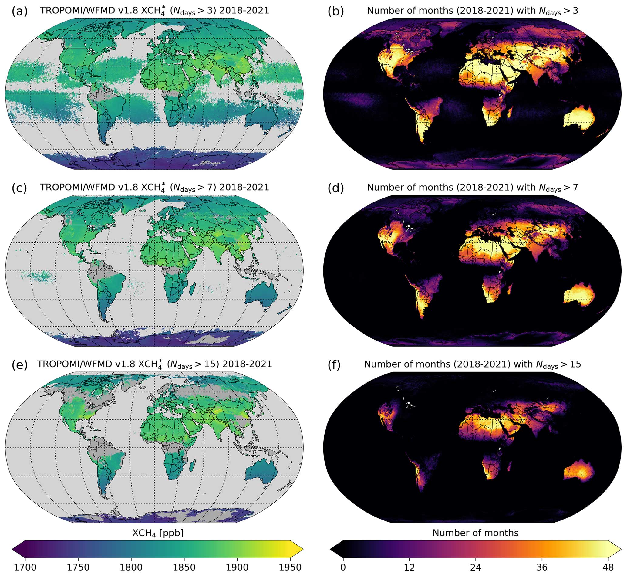
Figure A1 (a, c, e) 2018–2021 filtered XCH₄* calculated from monthly means in which the number of days of TROPOMI measurements within the month (N_days) is at least (a) 4 (as Fig. 2b), (c) 8 and (e) 16. (b, d, f) The corresponding number of months contributing to the multi-year mean.