Beyond self-healing: stabilizing and destabilizing photochemical adjustment of the ozone layer

The ozone layer is often noted to exhibit self-healing, whereby depletion of ozone aloft induces ozone increases below, explained as resulting from enhanced ozone production due to the associated increase in ultraviolet (UV) radiation below. Similarly, ozone enhancement aloft can reduce ozone below (reverse self-healing). This paper considers self-healing and reverse self-healing to manifest a general mechanism we call photochemical adjustment, whereby ozone perturbations lead to a downward cascade of anomalies in UV and ozone. Conventional explanations for self-healing imply that photochemical adjustment is stabilizing, damping perturbations towards the surface. However, photochemical adjustment can be destabilizing if the enhanced UV disproportionately increases the ozone sink, as can occur if the enhanced UV photolyzes ozone to produce atomic oxygen, which speeds up catalytic destruction of ozone. We analyze photochemical adjustment in two linear ozone models (Cariolle v2.9 and LINOZ), finding that (1) photochemical adjustment is destabilizing above 40 km in the tropical stratosphere and (2) self-healing often represents only a small fraction of the total photochemical stabilization. The destabilizing regime above 40 km is reproduced in a much simpler model: the Chapman cycle augmented with destruction of O and O₃ by generalized catalytic cycles and transport (the Chapman+2 model). The Chapman+2 model reveals that photochemical destabilization occurs where the ozone sink is more sensitive than the source to perturbations in overhead column ozone, which is found to occur when the window of overlapping absorption by O₂ and O₃ is optically unsaturated, i.e., when overhead slant column ozone is below approximately 10¹⁸ molec. cm⁻².

1 Introduction

The ozone layer and ultraviolet (UV) fluxes are tightly coupled. UV radiation photolyzes O₂ into atomic oxygen, which can then bond with O₂ to form O₃. UV is also strongly absorbed by the ozone that has been formed. This absorption protects life at the surface while also photolyzing the O₃, reversing the formation reaction and feeding back onto the structure of the ozone layer. Thus does the absorption of UV lead to the continuous destruction and reformation of the ozone layer, in the process attenuating the incoming UV flux at certain wavelengths by more than 30 orders of magnitude.

The coupling between UV and O₃ can lead to counterintuitive responses to perturbations. As was perhaps first noted by Johnston (1972), emitting an ozone-depleting substance whose local chemical effects strictly reduce ozone can nonetheless cause ozone to increase at certain altitudes (subsequent treatments: Hartmann, 1978; Dütsch, 1979; WMO, 1985; Solomon et al., 1985; Fomichev et al., 2007; Meul et al., 2014). This phenomenon is known as self-healing. Figure 1a provides a canonical example of self-healing in response to ozone-depleting substances (specifically, halocarbons including CFCs). The self-healing effect is visible as increases in O₃ in the tropical lower stratosphere and tropical tropopause layer. Similarly, perturbations that locally increase O₃ can lead to decreases in O₃ known as reverse self-healing (Groves et al., 1978; Haigh and Pyle, 1982; Jonsson et al., 2004; WMO, 2018). Figure 1b provides a canonical example of reverse self-healing in response to stratospheric cooling from the direct radiative effects of elevated CO₂, the cooling from which changes collisional reaction rates to generally increase O₃, which then leads to reductions in the tropical lower stratosphere (op. cit.).

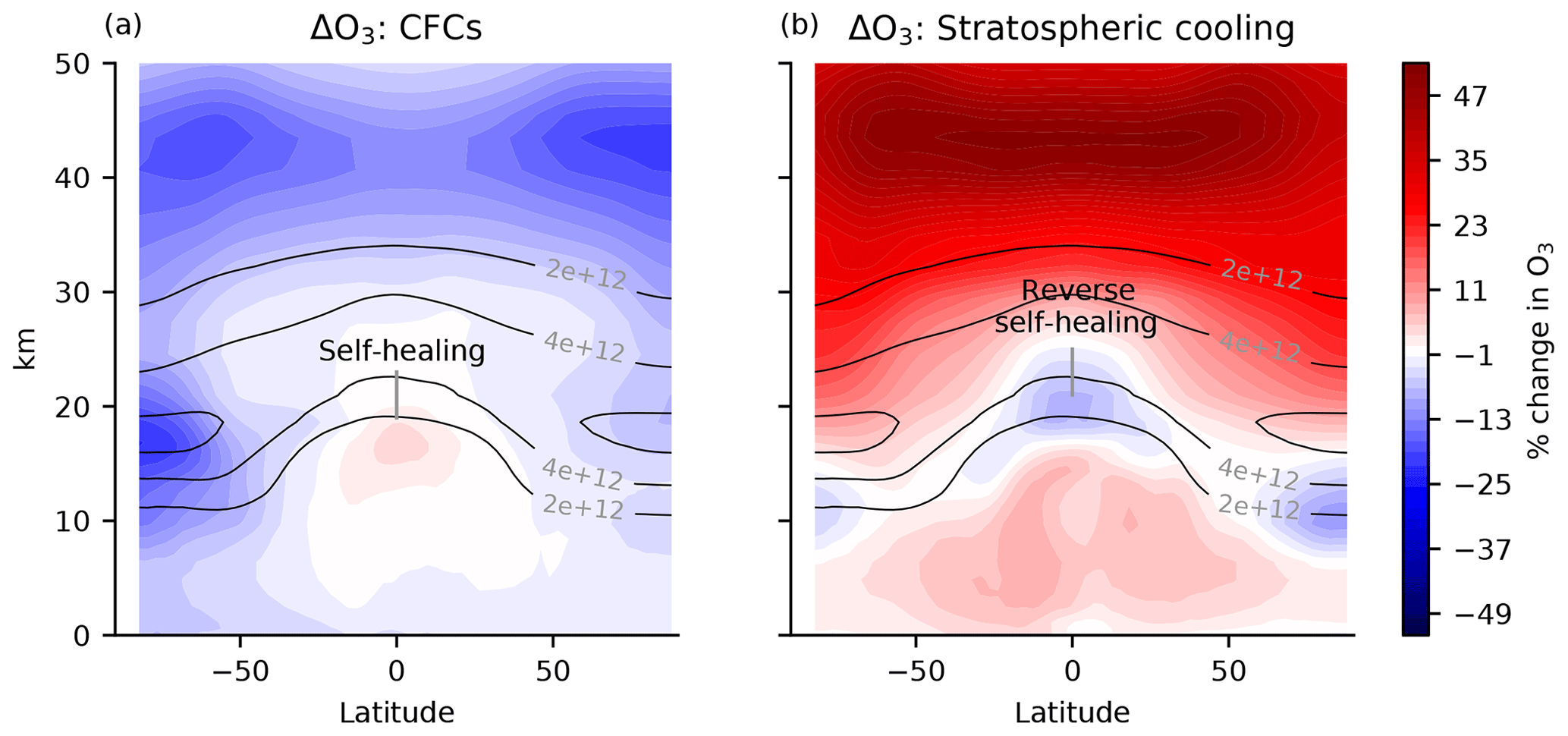
Figure 1 Canonical examples of self-healing and reverse self-healing. (a) Percent change in ozone in response to 2014 halocarbons (which include CFCs) imposed on a preindustrial atmosphere (piClim-HC minus piControl) in MRI-ESM2-0, accessed from the CMIP6 archive (Yukimoto et al., 2019). The halocarbons generally reduce ozone, in particular also in the polar night vortex. However, in the tropical lower stratosphere, ozone increases (self-healing). Preindustrial control ozone is contoured in solid lines (molec. cm⁻³). (b) The ozone response to stratospheric cooling from a quadrupling of CO₂ with preindustrial sea surface temperature (SST) (piClim-4xCO2 minus piControl) in MRI-ESM2-0 is accessed from the CMIP6 archive (Yukimoto et al., 2019). Stratospheric cooling generally increases ozone, except in the lower stratosphere, where there is reverse self-healing. The increases in tropospheric ozone are due to processes not discussed here.

Self-healing and reverse self-healing have been invoked in hundreds of papers, covering the ozone layer response to perturbations ranging from CFCs (e.g., NAS, 1976) and stratospheric cooling (e.g., Groves et al., 1978) to atmospheric oxidation (e.g., conceptually in Kasting and Donahue, 1980). However, despite being frequently invoked, self-healing and reverse self-healing are typically treated as curiosities only needed to explain unexpectedly signed responses of ozone to perturbations. They are only explained qualitatively, even in textbooks (e.g., Andrews et al., 1987; Finlayson-Pitts and Pitts, 2000).

Self-healing is typically explained as resulting from ozone depletion aloft, such as from CFCs, allowing photons that would have been absorbed aloft to penetrate more deeply into the atmosphere, photolyzing O₂ down below to increase the source and concentration of O₃ (self-healing). This mechanism relies on the spectral overlap between absorption by O₃ and O₂ at wavelengths less than 240 nm (e.g., Crutzen, 1974). The increased ozone from self-healing partially stabilizes the downwelling ultraviolet flux against the initial depletion of ozone. Reverse self-healing is explained as resulting because ozone enhancement aloft, such as from stratospheric cooling, blocks photons that would have been absorbed by O₂ below, reducing the source and concentration of O₃ below. Both self-healing and reverse self-healing partially stabilize the downwelling ultraviolet flux against the initial depletion of ozone and are shown schematically in the top row of Fig. 2.

This standard explanation neglects the sensitivity of the ozone sink to perturbations in UV fluxes. One reason that the ozone sink has been neglected is that photolysis of O₃ is typically considered to have a neutral effect on the ozone layer. This is because photolysis of O₃ liberates an atomic oxygen that typically bonds with O₂ to reform O₃, completing a null cycle. Because the atomic oxygen is prone to reforming O₃, it is usual to analyze ozone photochemistry in terms of odd oxygen (O_x ≡ O + O₃), which is longer-lived than ozone and preserved by photolysis of O₃ (e.g., Jacob, 1999; Brasseur and Solomon, 2005). However, this null cycle does not close perfectly, and leakage from the null cycle occurs if the atomic oxygen bonds with O₃ (as in Chapman, 1930) or, as happens more often, with catalysts of O₃ depletion such as HO₂ or NO₂ (Bates and Nicolet, 1950; Crutzen, 1970). Although small compared to the null cycle, this leakage means that UV can drive a photolytic sink of O₃. In other words, although odd oxygen is preserved by photolysis of O₃, the sink of odd oxygen is nonetheless sensitive to such photolysis.

The photolytic sink of O₃ opens up unconventional possibilities for the O₃ response to perturbations in overhead column O₃. If at some altitude the photolytic sink of ozone is more sensitive than the photolytic source, then O₃ depletion aloft would lead to a net enhancement of the O₃ sink below, further depleting O₃ below (self-amplified destruction). Likewise, O₃ addition aloft would lead to a net reduction in the O₃ sink below, further adding O₃ below (self-amplified production). Both of these responses are photochemically destabilizing, causing photochemical perturbations to amplify towards the surface. Figure 2 (bottom row) illustrates these two mechanisms of photochemical destabilization.

Photochemical destabilization has been noted before in Hartmann (1978), who identified significant photochemical destabilization above 40 km in a modified Chapman cycle model. However, they disclaimed their results as unrealistic, and these have since been neglected, perhaps for two main reasons: (1) they were considered theoretically impossible due to conceptual neglect of the photolytic sink of O₃, and (2) they were hiding, because self-healing and reverse self-healing demand an explanation by virtue of their unexpected sign compared to that of the initial perturbation, whereas photochemical destabilization does not change the sign of the ozone response to a perturbation.

We find that photochemical destabilization is not only theoretically possible but is also actually revealed in the coefficients of two linear ozone models (Cariolle v2.9 and LINOZ) in the tropical stratosphere above 40 km, exactly where it was first noted in Hartmann (1978) (Sect. 2). To better characterize these sensitivities, we generalize photochemical stabilization and destabilization as manifesting the broader phenomenon of photochemical adjustment, defined as the component of the O₃ response to a perturbation that is mediated by changes in UV from overhead column O₃ responses to that same perturbation (Sect. 3). Photochemical adjustment is quantified by the difference between the response to a perturbation under interactive versus locked UV. The region of photochemical destabilization above 40 km is then reproduced in a highly simplified model of the Chapman cycle augmented with two generalized sinks of O and O₃ to represent catalytic cycles and transport – the Chapman+2 model (Sect. 4). The Chapman+2 model facilitates the development of a theory for the transition altitude between photochemical destabilization and photochemical stabilization (Sect. 5). This theory reproduces the latitudinal structure of the region of photochemical destabilization. In Sect. 6, we develop a new qualitative explanation for photochemical adjustment that is consistent with these quantitative insights.

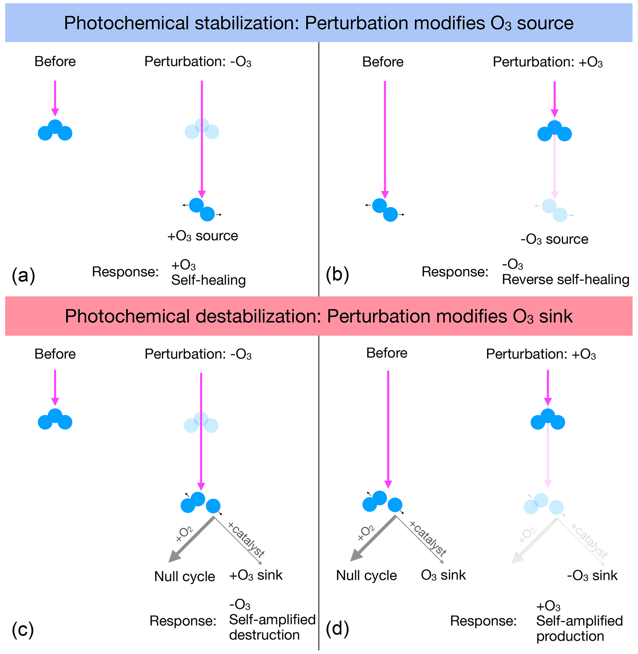
Figure 2 (a, b) Photochemical stabilization is typically explained as follows. (a) Depleting O₃ aloft allows deeper penetration of UV that photolyzes O₂ to increase the O₃ source and add O₃, causing self-healing. (b) Adding O₃ aloft blocks deeper penetration of UV, decreasing the photolysis of O₂ to decrease the O₃ source below, depleting O₃ and causing reverse self-healing. (c, d) Photochemical destabilization is proposed as follows. (c) Depleting O₃ aloft allows deeper penetration of UV that can increase photolysis of O₃, primarily driving a null cycle but with leakage that speeds up catalytic destruction of O, enhancing the ozone sink and further depleting ozone (self-amplified destruction). (d) Adding ozone aloft blocks deeper penetration of UV, which would have driven this catalytic destruction of O, the reduction of which reduces the O₃ sink below and adds further O₃ (self-amplified production).

2 Photochemical regimes in linear ozone models

To assess whether the ozone layer is photochemically stabilizing or destabilizing at a given location, we evaluate the sensitivity of the local net production rate of ozone (production minus loss) to a UV perturbation induced by a change in overhead column O₃, keeping all else fixed (including tendencies from transport). Increasing the overhead column O₃ decreases the photons reaching a given altitude in accordance with the spectrally varying absorption of ozone and the magnitude of the perturbation, reducing the photolysis rates of both O₂ and O₃ that drive the net production rate. If the increase in overhead column O₃ reduces the net production rate, this leads to photochemical stabilization. If the increase in overhead column O₃ increases the net production rate, this leads to photochemical destabilization. To characterize a climatology of photochemical regimes, this test must be repeated at all latitudes, altitudes, and seasons.

This exact battery of tests has been performed in chemical transport models by previous studies that developed linear ozone models, two independent coefficient sets of which are used throughout this study: Cariolle v2.9 (Cariolle and Déqué, 1986; Cariolle and Teyssèdre, 2007) and LINOZ (McLinden et al., 2000). Linear ozone models are tools for computationally speeding up chemistry–climate modeling of ozone. In a linear ozone model, the net tendencies of ozone from a chemical transport model with tens to hundreds of (photo)chemical reactions are linearized with respect to finite perturbations in local ozone concentration, temperature, and overhead column ozone. Then, for computational efficiency, the ozone module can be replaced with these linear functions evaluated using their table of coefficients. A standard linear ozone model equation, first proposed in Cariolle and Déqué (1986), is as follows:

$$\begin{array}{}\text{(1)}& {\displaystyle \frac{\mathrm{d}{r}_{{\text{O}}_{\mathrm{3}}}}{\mathrm{d}t}}=A_{\mathrm{1}}+A_{\mathrm{2}}(r_{{\text{O}}_{\mathrm{3}}}-A_{\mathrm{3}})+A_{\mathrm{4}}(T-A_{\mathrm{5}})+A_{\mathrm{6}}({\mathit{\chi }}_{{\text{O}}_{\mathrm{3}}}-A_{\mathrm{7}}),\end{array}$$

where $r_{{\text{O}}_{\mathrm{3}}}$ is the ozone mixing ratio, $A_{\mathrm{1}}=P-L$ is the basic-state photochemical production minus the loss rate, $A_{\mathrm{2}}=\partial (P-L)/\partial r_{{\text{O}}_{\mathrm{3}}}$, A₃ is the basic-state ozone mixing ratio, $A_{\mathrm{4}}=\partial (P-L)/\partial T$, A₅ is the basic-state temperature, $A_{\mathrm{6}}=\partial (P-L)/\partial {\mathit{\chi }}_{{\text{O}}_{\mathrm{3}}}$ where ${\mathit{\chi }}_{{\text{O}}_{\mathrm{3}}}$ is the overhead column ozone ${\int }_z^{\mathrm{\infty }}\left[{\text{O}}_{\mathrm{3}}\right]\mathrm{d}z$ (molec. cm⁻²) and [O₃] is the ozone number density (molec. cm⁻³), and A₇ is the basic-state overhead column ozone.

The linear ozone model coefficients are interpreted as classifying the photochemical regime based on the sign of the sensitivity to perturbations in column ozone (A₆). Photochemical stabilization occurs where A₆<0, meaning that an increase in overhead ozone reduces the net ozone production. Photochemical destabilization occurs where A₆>0, meaning that an increase in overhead ozone increases the net ozone production.

Previous studies have calculated the A parameters within chemical transport models as functions of altitude, latitude, and month. We have globally analyzed the A₆ coefficients in two models. The first (and primary) linear ozone model we evaluate is the Cariolle v2.9 linear ozone model (coefficients obtained by personal communication with Daniel Cariolle). The Cariolle linear ozone model is linearized with respect to the chemical transport model MOBIDIC first described in Cariolle and Brard (1984). MOBIDIC is driven by two-dimensional transport based on the residual circulation. The first linear ozone model was described in Cariolle and Déqué (1986), from which the Cariolle v2.9 linear ozone model descended, with a major update to specify the two-dimensional circulation from the ARPEGE-Climat model (Déqué et al., 1994) and to include heterogeneous chemistry in Cariolle and Teyssèdre (2007). The recent version of MOBIDIC to which the Cariolle v2.9 linear ozone model is calibrated includes the main gas-phase reactions driving the NO_x, HO_x, ClO_x, and BrO_x catalytic cycles, with 30 transported long-lived species and 30 short-lived species computed diagnostically (Cariolle and Teyssèdre, 2007). The Cariolle linear ozone model has been shown to perform well compared to state-of-the-art comprehensive chemistry–climate models (Meraner et al., 2020) and is used to prognose ozone in the ERA5 reanalysis (Hersbach et al., 2020). The second linear ozone model we evaluate is the LINOZ scheme, based on the UC Irvine chemical transport model (e.g., as used in Hall and Prather, 1995) driven by the general circulation from NASA GISS ModelE (coefficients obtained by personal communication with Clara Orbe). LINOZ is documented in McLinden et al. (2000), and recent implementations include Rind et al. (2014) and DallaSanta et al. (2021).

The values of A₆ during the month of March (chosen as an equinoctial month) are shown for Cariolle v2.9 and LINOZ in Fig. 3a, b. Negative values indicate photochemical stabilization, and positive values indicate photochemical destabilization. A major result is that there is significant and large photochemical destabilization, primarily above 40 km. This means that ozone depletion above 40 km removes additional ozone down to 40 km. Because these two linear ozone models agree so strongly, further analyses will focus on the Cariolle v2.9 model unless otherwise stated.

Photochemical destabilization occurs well above the bulk of the ozone layer; as evaluated using the climatological structure of O₃ in the Cariolle v2.9 coefficients, 4 % of ozone molecules in the deep tropics (from 20° S to 20° N) are in a photochemically destabilizing regime above 40 km. Despite including only a modest fraction of O₃, this region of photochemical destabilization challenges the prevailing theory, which only emphasizes the photochemical sensitivity of the ozone source and therefore cannot account for destabilization.

Intriguingly, the photochemical destabilization above 40 km in the tropics is located where it was first noted by Hartmann (1978) in their modified Chapman cycle model. We reproduce the transition from destabilization aloft to stabilization below in our own version of the Chapman cycle augmented with generalized sinks of O and O₃ from transport and catalytic cycles. These sinks are represented as two generalized chemical reactions, and hence our model is called the Chapman+2 model. The photochemical sensitivity of the Chapman+2 model is shown in Fig. 3c, which reproduces key features from the linear ozone models, which are in turn based on much more complex photochemical models. The details of the Chapman+2 model results will be presented later in Sect. 4.

Figure 3 Sensitivity of the net odd-oxygen photochemical production rate to perturbations in column ozone, calculated for the month of March (approximately equinoctial conditions such that latitude θ ≈ solar zenith angle) in two linear ozone models: (a) Cariolle v2.9 based on MOBIDIC (Cariolle and Déqué, 1986) and (b) LINOZ based on the UC Irvine chemical transport model (CTM) driven by NASA GISS ModelE (McLinden et al., 2000). The linear ozone model coefficients are compared to the Chapman+2 model, in which latitudinal dependence is represented by performing single-column calculations. Photochemical stabilization is indicated by negative values, whereas photochemical destabilization is indicated by positive values. Spectrally resolved photochemical theory (Sect. 5) predicts positive coefficients where the slant ozone column is less than 10¹⁸ molec. cm⁻² (i.e., above the magenta curve).

The coefficients of the Cariolle v2.9 linear ozone model have provided exactly the evidence needed to classify regions of the atmosphere as photochemically stabilizing or destabilizing. One striking feature of Fig. 3a, b is that the sensitivity of the net ozone production rate to perturbations in column ozone has a larger magnitude in the destabilizing region than in the stabilizing region. This might seem to imply that destabilization is stronger than stabilization. However, the basic-state production and loss are also larger in the upper atmosphere, where the UV flux has not been attenuated as strongly, so therefore the ozone equilibration timescale may also be relevant to considering the magnitude of photochemical stabilization. Questions about the magnitude of photochemical stabilization demand a method to quantify the full vertical profile of photochemical adjustment in general, which is developed in the following section.

3 Defining photochemical adjustment and quantifying it using a linear ozone model

The idea behind photochemical stabilization or destabilization is that changes in ozone aloft can lead to a downward cascade of perturbations in ozone, yet this idea has not been previously formalized in a quantitative way. Here, we define photochemical adjustment as the component of the ozone response to a perturbation that results from changes in photolysis due to changes in column ozone aloft. Photochemical adjustment is therefore quantified as the difference between a fully interactive simulation of ozone photochemistry in which ozone and UV are coupled in the column through the photolysis rates, compared to one where the UV fluxes (and hence photolysis rates) are locked at their unperturbed values:

$$\begin{array}{}\text{(2)}& \begin{array}{rl}\text{photochemical adjustment}& \equiv \left[{\text{O}}_{\mathrm{3}}\right]{|}_{\text{fully interactive}}\\ & -\left[{\text{O}}_{\mathrm{3}}\right]{|}_{\text{UV-locked}}.\end{array}\end{array}$$

This UV-locking method can in principle be implemented in any modeling context for atmospheric chemistry. Intuitively, a UV-locked simulation can be obtained in a photochemical model by locking the overhead column ozone when calculating photolysis rates, where the locked ozone could be steady or climatologically evolving, depending on the context. This ensures that the photolysis rates do not respond to any changes in ozone resulting from the perturbation, but it allows all other photochemical responses.

In this paper, we implement this approach using two methods. First, we use the Cariolle v2.9 linear ozone model coefficients to develop a linear emulator of photochemical adjustment. Later, we will perform various UV-locking experiments in the Chapman+2 model, which will be shown to reproduce essential results from the linear ozone model. Both of these analyses consider the equilibrated response to steady perturbations.

We begin our derivation for the linear emulator of the perturbation ozone equation by converting ozone anomalies in the linear ozone model from mixing ratio (Eq. 1) to number density (for convenience) by multiplying by the number density of air, denoted as n_a (molec. cm⁻³). We then decompose the variables in our prognostic ozone number density equation into basic-state and perturbation components, $x=\stackrel{\mathrm{‾}}{x}+x^{\prime }$, where $\stackrel{\mathrm{‾}}{x}$ is the basic-state component and x^′ is the perturbation. Subtracting the basic-state component from the total equation and assuming a quasi-steady state, we solve for the perturbation ozone number density as a function of height in the presence of some prescribed perturbation, G:

$$\begin{array}{}\text{(3)}& [{\text{O}}_{\mathrm{3}}{]}^{\prime }=-{\displaystyle \frac{A_{\mathrm{4}}{n}_{\mathrm{a}}{T}^{\prime }}{A_{\mathrm{2}}}}-{\displaystyle \frac{A_{\mathrm{6}}{n}_{\mathrm{a}}{\mathit{\chi }}_{{\text{O}}_{\mathrm{3}}}^{\prime }}{A_{\mathrm{2}}}}+G.\end{array}$$

On the right-hand side, the first term captures the sensitivity to temperature perturbations, the second term captures the sensitivity to overhead column ozone perturbations (thereby coupling in the photochemical adjustment), and the third term is the prescribed perturbation in ozone. A₂ (defined as $\partial (P-L)/\partial r_{{\text{O}}_{\mathrm{3}}}$) tends to be negative, reflecting the fact that local perturbations in ozone tend to decay on a timescale of $\mathrm{-}\mathrm{1}/A_{\mathrm{2}}$. Although Eq. (3) is linear at any given height, it is mathematically implicit because the perturbation overhead column ozone is the integral of the ozone number density perturbation (i.e., ${\mathit{\chi }}_{{\text{O}}_{\mathrm{3}}}^{\prime }={\int }_z^{\mathrm{\infty }}[{\text{O}}_{\mathrm{3}}{]}^{\prime }\mathrm{d}z$). Photochemical adjustment at height thus influences lower levels, introducing a spatial nonlinearity encoded in the A₆ term, and Eq. (3) must be solved from the top of the atmosphere downwards.

We assess the response of tropical ozone to highly idealized forcing by ozone depletion (e.g., from ozone-depleting substances) and stratospheric cooling (e.g., from the direct radiative effects of CO₂). The response to such perturbations is generally known to have a nontrivial vertical structure (e.g., Fig. 1), although this response already includes the effects of photochemical adjustment, whose structure we seek to isolate. In order to illustrate how photochemical adjustment can induce a nontrivial vertical structure even in response to uniform perturbations, we consider constant (or piecewise-constant) perturbations. Ozone depletion is represented as a uniform reduction of ozone below its basic-state value ($G=-G_{\mathrm{0}}$, $T^{\prime }=\mathrm{0}$), which in turn can induce photochemical perturbations by perturbing the UV flux that drives ozone at lower levels. Thus, the fully interactive linear response to this uniform perturbation in ozone includes the perturbation itself plus the nonlocal effects of perturbed UV flux. Stratospheric cooling is represented as a uniform cooling (G=0, $T^{\prime }=-\mathrm{\Delta }T$), which tends to locally increase ozone. This cooling is imposed uniformly, even extending into the troposphere, where the response is small but should not be considered a realistic response to elevated CO₂, which instead (as is well known) warms the troposphere. The local increases in ozone from these perturbations then perturb the UV fluxes, leading to a fully interactive response that includes the local effects of cooling and the nonlocal effects of changes in overhead column ozone.

These two perturbations are explored by using the coefficients of the linear ozone model to perform an offline calculation of the response of a steady-state ozone layer to ozone depletion or stratospheric cooling. The linear ozone model distills the relative importance of the local effects of these perturbations from the nonlocal effects of the UV flux perturbations from aloft, as conveyed by the linear sensitivity to overhead column ozone. Both of these offline calculations have been performed on the discrete grid of the Cariolle v2.9 linear ozone model, with levels z_i, $i=\mathrm{1},\mathrm{2},\mathrm{\dots },N$ (where N=91) numbered from the top of the atmosphere downwards, each with a thickness of Δz_i ranging from >3 km above 55 km to less than 1 km below the ozone maximum around 26 km. Uniform ozone depletion with a magnitude G₀ has been imposed at and below z₅=60 km. The fully interactive ozone response to this perturbation has been calculated by iterating between calculating the ozone response at level i and the resulting overhead column ozone anomaly at level i that is then seen by level i+1. The initial anomaly is therefore $\left[{\text{O}}_{\mathrm{3}}{]}^{\prime }\right(z_{\mathrm{5}})=-G_{\mathrm{0}}$, which leads to an overhead column ozone anomaly of ${\mathit{\chi }}_{{\text{O}}_{\mathrm{3}}}^{\prime }\left(z_{\mathrm{5}}\right)=-G_{\mathrm{0}}\mathrm{\Delta }{z}_{\mathrm{5}}$. The fully interactive response at z₆ can then be calculated as $\left[{\text{O}}_{\mathrm{3}}{]}^{\prime }\right(z_{\mathrm{6}})=-G_{\mathrm{0}}-A_{\mathrm{6}}{n}_{\mathrm{a}}{\mathit{\chi }}_{{\text{O}}_{\mathrm{3}}}^{\prime }(z_{\mathrm{5}})/A_{\mathrm{2}}$. This ozone anomaly is used to update the overhead column ozone perturbation as ${\mathit{\chi }}_{{\text{O}}_{\mathrm{3}}}^{\prime }\left(z_{\mathrm{6}}\right)={\mathit{\chi }}_{{\text{O}}_{\mathrm{3}}}^{\prime }\left(z_{\mathrm{5}}\right)+\left[{\text{O}}_{\mathrm{3}}{]}^{\prime }\right(z_{\mathrm{6}})\mathrm{\Delta }{z}_{\mathrm{6}}$. The solution can then proceed iteratively, where at each lower altitude we first calculate the ozone perturbation and then add that ozone perturbation (multiplied by the layer thickness) to the overhead column ozone perturbation. In this way, our calculation is locally linear in the overhead column ozone perturbation, but the dependence on overhead column ozone means that the ozone response at any given altitude depends nonlocally on the changes aloft.

A similar iterative method is used to calculate the response to stratospheric (and tropospheric) cooling. Our iterative calculation begins at the top of the model (z₁=80 km) with a local ozone anomaly of $\left[{\text{O}}_{\mathrm{3}}{]}^{\prime }\right(z_{\mathrm{1}})=A_{\mathrm{4}}{n}_{\mathrm{a}}\mathrm{\Delta }T/A_{\mathrm{2}}$. This local ozone anomaly leads to an overhead column ozone perturbation of ${\mathit{\chi }}_{{\text{O}}_{\mathrm{3}}}^{\prime }\left(z_{\mathrm{1}}\right)=\left[{\text{O}}_{\mathrm{3}}{]}^{\prime }\right(z_{\mathrm{1}})\mathrm{\Delta }{z}_{\mathrm{1}}$. The ozone perturbation at the next lower altitude can then be calculated in general as $\left[{\text{O}}_{\mathrm{3}}{]}^{\prime }\right(z_i)=A_{\mathrm{4}}{n}_{\mathrm{a}}\mathrm{\Delta }T/A_{\mathrm{2}}-A_{\mathrm{6}}{n}_{\mathrm{a}}{\mathit{\chi }}_{{\text{O}}_{\mathrm{3}}}^{\prime }(z_{i-\mathrm{1}})/A_{\mathrm{2}}$. The overhead column ozone perturbation can then be updated in general as ${\mathit{\chi }}_{{\text{O}}_{\mathrm{3}}}^{\prime }\left(z_i\right)={\mathit{\chi }}_{{\text{O}}_{\mathrm{3}}}^{\prime }\left(z_{i-\mathrm{1}}\right)+\left[{\text{O}}_{\mathrm{3}}{]}^{\prime }\right(z_i)\mathrm{\Delta }{z}_i$.

Using this approach, we calculated the linear response of ozone to uniform ozone depletion and stratospheric cooling. The response to these perturbations in the absence of photochemical adjustment can also be calculated directly as the UV-locked response by repeating the calculation with ${\mathit{\chi }}_{{\text{O}}_{\mathrm{3}}}^{\prime }$ overwritten to zero everywhere. For uniform ozone depletion, the UV-locked response is simply the prescribed ozone depletion, a reduction by G₀ at all altitudes below 60 km. For stratospheric cooling, the UV-locked response is the direct thermal response given by the first term on the right-hand side of Eq. (3). Knowing the UV-locked responses, it is then straightforward to calculate the photochemical adjustment, which (per Eq. 2) is the fully interactive response minus the UV-locked response.

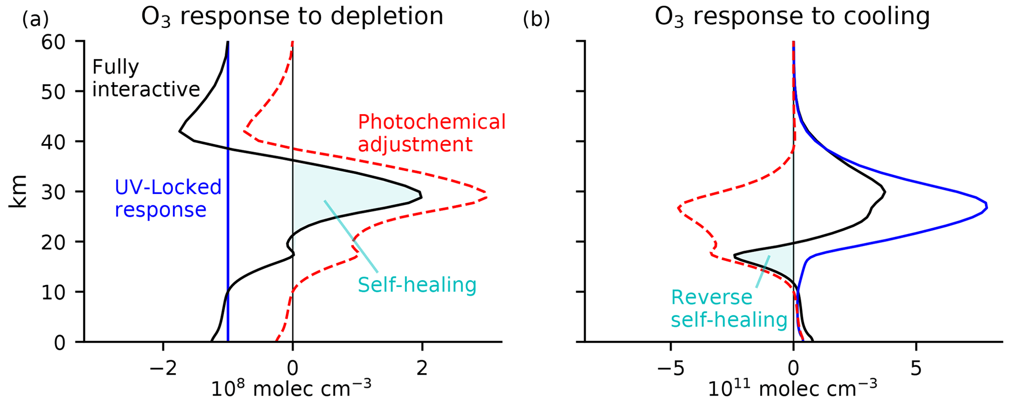
Figure 4 Equatorial ozone response to (a) uniform depletion by 10⁸ molec. cm⁻³ everywhere below 60 km and (b) uniform cooling of 10 K. The calculation is performed by iteratively solving Eq. (3) using equatorial coefficients from the Cariolle v2.9 linear ozone model. The fully interactive response (black) is decomposed into a UV-locked response (blue) and photochemical adjustment (red). Self-healing and reverse self-healing (cyan shading) are merely the tip of the iceberg of large photochemical adjustment throughout the column, with photochemical destabilization above 40 km and photochemical stabilization below 40 km.

The results are shown in Fig. 4, as calculated using the linear ozone model coefficients in March for an equatorial atmospheric column. The response to uniform ozone depletion below 60 km of G₀=10⁸ molec. cm⁻³ is shown in Fig. 4a, with the prescribed depletion shown in blue. The fully interactive response (black) differs substantially from the prescribed perturbation. The fully interactive response shows reductions in ozone in the upper stratosphere that are larger in magnitude than those prescribed, peaking at 42 km with an amplitude 75 % larger than what is prescribed. This is a consequence of self-amplified destruction in the region of photochemical destabilization above 40 km. Below 40 km, the response is no longer photochemically destabilizing, and the fully interactive response is more positive than the prescribed reduction. At 35 km, the fully interactive response becomes positive in absolute terms – self-healing. The absolute increase in ozone peaks at a value around 2G₀ at 29 km; the associated photochemical adjustment here is 3G₀. The photochemical adjustment decays towards the lower stratosphere and troposphere, where the ozone response eventually resembles the prescribed depletion. By integrating these curves, it is evident that the overall column response of ozone is substantially modified by photochemical adjustment. The column integral of the prescribed perturbation is $-G_{\mathrm{0}}\times \mathrm{60}$ km, whereas the column integral of the fully interactive response is only half as large. Thus, photochemical adjustment significantly compensates for the initial perturbation.

The response to a uniform stratospheric cooling of ΔT=10 K is shown in Fig. 4b. The UV-locked response (blue) is a strict increase in ozone. Cooling approximately re-scales ozone by a constant factor, so the ozone response is shaped approximately like the unperturbed ozone profile. The fully interactive response (black) differs substantially from the UV-locked response, especially in the lower stratosphere. The maximum increase in ozone is predicted in both cases to occur around 30 km, but the fully interactive response is only half that predicted under UV locking. This discrepancy is due to photochemical adjustment, which is large and stabilizing throughout much of the stratosphere. Below 20 km, ozone is reduced in absolute terms (reverse self-healing). Integrating the column responses, the increase in total column ozone in the fully interactive case is only 43 % as large as the increase in the UV-locked case. Again, photochemical adjustment has halved the perturbation compared to in its absence.

A major result of this analysis is that photochemical adjustment is large and significant throughout the stratosphere and not just in the lower stratosphere, where self-healing and reverse self-healing tend to be found. It is important here to distinguish between photochemical adjustment and self-healing or reverse self-healing. We can express the colloquial definition of self-healing or reverse self-healing as follows:

$$\mathrm{\text{(reverse) self-healing}}\equiv \left\{\begin{array}{ll}[{\text{O}}_{\mathrm{3}}{]}_{\text{fully interactive}}^{\prime }& \text{if }\\ \mathrm{sign}\left(\right[{\text{O}}_{\mathrm{3}}{]}_{\text{fully interactive}}^{\prime })\\ \cdot \mathrm{sign}\left(\right[{\text{O}}_{\mathrm{3}}{]}_{\text{UV-locked}}^{\prime })<\mathrm{0},\\ \mathrm{0}& \text{otherwise.}\end{array}\right.$$

This definition shows that self-healing and reverse self-healing are given by the ozone perturbation in a fully interactive simulation wherever the ozone anomaly has the opposite sign to what is expected from the imposed perturbation. Expressed in this way, it is clear that self-healing and reverse self-healing are not the same as photochemical adjustment (defined in Eq. 2). Indeed, self-healing and reverse self-healing are often just the tip of the iceberg of much larger photochemical stabilization. This is especially clear in the response to stratospheric cooling (Fig. 4b), in which the column-integrated reverse self-healing is only 14 % as large as the column-integrated photochemical stabilization.

The two main results from this analysis of linear ozone models are that (1) photochemical adjustment is destabilizing above 40 km and (2) photochemical adjustment can be large throughout the stratosphere, which is much greater than implied by conventional self-healing and reverse self-healing. Photochemical destabilization is inconsistent with the standard explanation for self-healing and reverse self-healing and therefore demands a revision of the conceptual understanding of these ubiquitous phenomena. This new conceptual understanding will also provide quantitative insights.

4 Understanding photochemical adjustment using the Chapman+2 model

The large photochemical destabilization above 40 km and the large photochemical adjustment throughout the stratosphere (not merely in regions of self-healing or reverse self-healing) both demand a revision to present understanding. New understanding is challenging to achieve in comprehensive chemistry–climate models with tens of prognostic chemical species undergoing hundreds of reactions. However, some basic properties of photochemical adjustment do not depend on this complexity and are reproducible from simpler models. In particular, the prospect of photochemical destabilization was first raised in Hartmann (1978), who found such behavior in a modified version of the Chapman cycle above 40 km. It is at precisely those altitudes where the linear ozone models also simulate photochemical destabilization, suggesting that radically simplified photochemical models might support quantitative insights into photochemical adjustment.

We have analyzed photochemical adjustment in such a radically simplified model, the Chapman+2 model, which begins with the Chapman cycle but then augments it with two chemical reactions representing the generalized damping of ozone from sinks of O and O₃ due to catalytic cycles and transport. The Chapman+2 model is comprehensively introduced in recent work focusing on the structure of the ozone layer (Match et al., 2024), complementing our focus here on sensitivities. The Chapman+2 model was shown in Fig. 3 to reproduce the photochemical regimes from two chemical transport models. We now explain that calculation and use it to develop physical intuition and quantitative insights into photochemical adjustment.

4.1 Methods: the Chapman+2 model

The Chapman cycle considers the effects of ultraviolet radiation driving photochemical reactions of O, O₂, and O₃ (Chapman, 1930). It is the foundational model that first explained how photochemistry could lead to an ozone layer in the stratosphere. However, the Chapman cycle underestimates the ozone sink, which in the tropical stratosphere arises predominantly from catalytic cycles and transport. To restore the leading-order ozone sinks, and in line with theories of chemical families for the stratospheric ozone photochemistry (Brasseur and Solomon, 2005), we have augmented the Chapman cycle with two chemical reactions that represent generalized destruction of O and O₃ by catalytic cycles and transport, as follows:

$$\begin{array}{}\text{(R1)}& {\displaystyle }{\text{O}}_{\mathrm{2}}+h\mathit{\nu }\to \text{O}+\text{O}(\mathit{\lambda }<\mathrm{240}\text{nm}),\text{(R2)}& {\displaystyle }\text{O}+{\text{O}}_{\mathrm{2}}+\text{M}\to {\text{O}}_{\mathrm{3}}+\text{M},\text{(R3)}& {\displaystyle }{\text{O}}_{\mathrm{3}}+h\mathit{\nu }\to {\text{O}}_{\mathrm{2}}+\text{O}(\mathit{\lambda }<\mathrm{1080}\text{nm}),\text{(R4)}& {\displaystyle }\text{O}+{\text{O}}_{\mathrm{3}}\to \mathrm{2}{\text{O}}_{\mathrm{2}},\text{(R5)}& {\displaystyle }\text{O}\stackrel{{\text{Z}}_{\text{O}}}{\to }{\displaystyle \frac{\mathrm{1}}{\mathrm{2}}}{\text{O}}_{\mathrm{2}},\text{(R6)}& {\displaystyle }{\text{O}}_{\mathrm{3}}\stackrel{{\text{Z}}_{{\text{O}}_{\mathrm{3}}}}{\to }{\displaystyle \frac{\mathrm{3}}{\mathrm{2}}}{\text{O}}_{\mathrm{2}},\end{array}$$

where Reactions (R1)–(R4) are the classical Chapman cycle and Reactions (R5)–(R6) are the two additional generalized sinks. Reactions (R1) and (R3) are photolysis reactions, and M is a third body with the number density of air (n_a). The combination reactions proceed as the number density of the chemical reactants multiplied by a rate coefficient k_i, $i=\mathrm{2},\mathrm{4}$. For example, Reaction (R2) has a rate of k₂[O][O₂][M], which in general depends on temperature. The generalized reactions represent two sink pathways: destruction of odd oxygen can scale with atomic oxygen, as in Reaction (R5), which proceeds at the rate κ_O[O], or it can scale with ozone, as in Reaction (R6), which proceeds at the rate ${\mathit{\kappa }}_{{\text{O}}_{\mathrm{3}}}\left[{\text{O}}_{\mathrm{3}}\right]$.

For steady-state solutions to the Chapman cycle, the molar fraction of O₂ is several orders of magnitude larger than that of O and O₃ and will be treated as constant ($C_{{\text{O}}_{\mathrm{2}}}=\mathrm{0.21}$). Then, setting $\partial \text{O}/\partial t=\partial \left[{\text{O}}_{\mathrm{3}}\right]/\partial t=\mathrm{0}$, these reactions can be solved algebraically to yield a quadratic equation for O₃ at a given altitude:

$$\begin{array}{}\text{(4)}& \left[{\text{O}}_{\mathrm{3}}\right]={\displaystyle \frac{J_{{\text{O}}_{\mathrm{2}}}{k}_{\mathrm{2}}}{k_{\mathrm{4}}}}{C}_{{\text{O}}_{\mathrm{2}}}^{\mathrm{2}}{n}_{\mathrm{a}}^{\mathrm{3}}{\displaystyle \frac{\mathrm{1}}{\left(\begin{array}{c}{J}_{{\text{O}}_{\mathrm{3}}}\left[{\text{O}}_{\mathrm{3}}\right]+J_{{\text{O}}_{\mathrm{2}}}{C}_{{\text{O}}_{\mathrm{2}}}{n}_{\mathrm{a}}+\frac{{\mathit{\kappa }}_{{\text{O}}_{\mathrm{3}}}\left[{\text{O}}_{\mathrm{3}}\right]}{\mathrm{2}}\\ +\frac{J_{{\text{O}}_{\mathrm{3}}}{\mathit{\kappa }}_{\text{O}}}{\mathrm{2}{k}_{\mathrm{4}}}+\frac{k_{\mathrm{2}}{\mathit{\kappa }}_{{\text{O}}_{\mathrm{3}}}{C}_{{\text{O}}_{\mathrm{2}}}{n}_{\mathrm{a}}^{\mathrm{2}}}{\mathrm{2}{k}_{\mathrm{4}}}+\frac{{\mathit{\kappa }}_{\text{O}}{\mathit{\kappa }}_{{\text{O}}_{\mathrm{3}}}}{\mathrm{2}{k}_{\mathrm{4}}}\end{array}\right)}}.\end{array}$$

A similar derivation yields a diagnostic equation for atomic oxygen:

$$\begin{array}{}\text{(5)}& \left[\text{O}\right]={\displaystyle \frac{J_{{\text{O}}_{\mathrm{2}}}{C}_{{\text{O}}_{\mathrm{2}}}{n}_{\mathrm{a}}+J_{{\text{O}}_{\mathrm{3}}}\left[{\text{O}}_{\mathrm{3}}\right]+\frac{{\mathit{\kappa }}_{{\text{O}}_{\mathrm{3}}}\left[{\text{O}}_{\mathrm{3}}\right]}{\mathrm{2}}}{k_{\mathrm{2}}{C}_{{\text{O}}_{\mathrm{2}}}{n}_{\mathrm{a}}^{\mathrm{2}}+\frac{{\mathit{\kappa }}_{\text{O}}}{\mathrm{2}}}}.\end{array}$$

This photochemical system has been described in more detail in Match et al. (2024), which explains why the number density of ozone has an interior maximum in the tropical atmosphere.

Ozone appears implicitly on the right-hand side of Eq. (4) through the photolysis rates $J_{{\text{O}}_{\mathrm{2}}}$ (s⁻¹) and $J_{{\text{O}}_{\mathrm{3}}}$ (s⁻¹). Photolysis is governed by the spectrally integrated UV absorption:

$$\begin{array}{}\text{(6)}& {\displaystyle }{J}_{{\text{O}}_{\mathrm{2}}}\left(z\right)=\underset{\mathit{\lambda }}{\int }{q}_{{\text{O}}_{\mathrm{2}}}\left(\mathit{\lambda }\right){\mathit{\sigma }}_{{\text{O}}_{\mathrm{2}}}\left(\mathit{\lambda }\right)I_{\mathit{\lambda }}\left(z\right)\mathrm{d}\mathit{\lambda },\text{(7)}& {\displaystyle }{J}_{{\text{O}}_{\mathrm{3}}}\left(z\right)=\underset{\mathit{\lambda }}{\int }{q}_{{\text{O}}_{\mathrm{3}}}\left(\mathit{\lambda }\right){\mathit{\sigma }}_{{\text{O}}_{\mathrm{3}}}\left(\mathit{\lambda }\right)I_{\mathit{\lambda }}\left(z\right)\mathrm{d}\mathit{\lambda },\end{array}$$

with wavelength λ, quantum yield q_i(λ) (molecules decomposed per photon absorbed by species i), absorption coefficient σ_i (cm² molec⁻¹) (Fig. 5b), and UV flux density with respect to wavelength I_λ(z) (photons cm⁻² s⁻¹ nm⁻¹). The absorption of photons by photolysis attenuates the UV flux:

$$\begin{array}{}\text{(8)}& I_{\mathit{\lambda }}\left(z\right)=I_{\mathit{\lambda }}\left(\mathrm{\infty }\right)\exp \left(-{\displaystyle \frac{{\mathit{\tau }}_{\mathit{\lambda }}\left(z\right)}{\cos \mathit{\theta }}}\right),\end{array}$$

where I_λ(∞) is the incoming UV flux (Fig. 5a), θ is the solar zenith angle, and τ_λ is the optical depth as a function of wavelength. The optical depth at a given altitude depends on the column-integrated O₂ and O₃ above that level:

$$\begin{array}{}\text{(9)}& {\mathit{\tau }}_{\mathit{\lambda }}\left(z\right)={\mathit{\sigma }}_{{\text{O}}_{\mathrm{2}}}\left(\mathit{\lambda }\right){\mathit{\chi }}_{{\text{O}}_{\mathrm{2}}}\left(z\right)+{\mathit{\sigma }}_{{\text{O}}_{\mathrm{3}}}\left(\mathit{\lambda }\right){\mathit{\chi }}_{{\text{O}}_{\mathrm{3}}}\left(z\right),\end{array}$$

where ${\mathit{\chi }}_{{\text{O}}_{\mathrm{2}}}={\int }_z^{\mathrm{\infty }}\left[{\text{O}}_{\mathrm{2}}\right]\mathrm{d}z$ and ${\mathit{\chi }}_{{\text{O}}_{\mathrm{3}}}={\int }_z^{\mathrm{\infty }}\left[{\text{O}}_{\mathrm{3}}\right]\mathrm{d}z$.

The collisional reaction rates k₂ and k₄ are calculated with temperature-dependent values from Brasseur and Solomon (2005). The generalized sinks of O and O₃ proceed with damping rates representing both transport and catalytic cycles. Motivated by consideration of the tropical lower stratosphere, in which upwelling advects ozone-poor air up from below in order to damp O₃ (e.g., Match and Gerber, 2022), transport will be crudely parameterized as a constant damping of ${\mathit{\kappa }}_{{\stackrel{\mathrm{‾}}{w}}^{*}}=$ (3 months)⁻¹. Catalytic cycles will be parameterized by taking all (temperature-dependent) damping-like terms from the budget of generalized odd oxygen (O_y) of Brasseur and Solomon (2005). That is, terms of the form $\partial {\text{O}}_y/\partial t=-k\left[{\text{Z}}_{\text{O}}\right]\left[\text{O}\right]$ are taken to damp O, and terms of the form $\partial {\text{O}}_y/\partial t=-k\left[{\text{Z}}_{{\text{O}}_{\mathrm{3}}}\right]\left[{\text{O}}_{\mathrm{3}}\right]$ are taken to damp O₃ for catalysts Z_O and $Z_{{\text{O}}_{\mathrm{3}}}$. This leads to the following damping rates:

$$\begin{array}{}\text{(10)}& {\displaystyle }\begin{array}{rl}{\mathit{\kappa }}_{\text{O}}& ={\mathit{\kappa }}_{{\stackrel{\mathrm{‾}}{w}}^{*}}+a_{\mathrm{5}}\left[\text{OH}\right]+a_{\mathrm{7}}\left[{\text{HO}}_{\mathrm{2}}\right]+\mathrm{2}{b}_{\mathrm{3}}\left[{\text{NO}}_{\mathrm{2}}\right]+\mathrm{2}{d}_{\mathrm{3}}\left[\text{ClO}\right]\\ & +\mathrm{2}{e}_{\mathrm{3}}\left[\text{BrO}\right],\end{array}\text{(11)}& {\displaystyle }{\mathit{\kappa }}_{{\text{O}}_{\mathrm{3}}}={\mathit{\kappa }}_{{\stackrel{\mathrm{‾}}{w}}^{*}}+a_{\mathrm{2}}\left[\text{H}\right]+a_{\mathrm{6}}\left[\text{OH}\right]+a_{\mathrm{6}b}\left[{\text{HO}}_{\mathrm{2}}\right].\end{array}$$

The vertical profile of these damping rates is shown in Fig. 5c. To validate these damping rates, we also show the odd-oxygen damping timescale from the Cariolle v2.9 linear ozone model compared to the equivalent timescale implied in the Chapman+2 model (cyan curves). The chemical reactions that comprise the damping in the Chapman+2 model are intended to provide only an idealized representation of the global stratosphere while excluding photochemical reactions between the catalysts, heterogeneous chemistry in the polar stratosphere, and tropospheric chemistry. The simplified representation of transport is intended to provide an idealized representation of only the tropical lower stratosphere. These geographical caveats will be considered when using the Chapman+2 model to interpret the global results from the linear ozone models.

4.2 Chapman+2 model numerics

We use the Chapman+2 model as implemented in Match et al. (2024). This solution is solved for a steady-state, isothermal atmosphere and a default of overhead Sun (cos θ=1). We neglect scattering, clouds, and surface reflection. Equation (4) is solved at each altitude downward from the top of the atmosphere to calculate the photochemical equilibrium profile.

The vertical dimension is discretized into vertical levels (Δz=100 m) ranging from the surface to 100 km. The idealized shortwave radiative transfer and photolysis rates are solved on a wavelength grid with 621 discretized wavelengths ranging from 180 to 800 nm. Spectrally resolved parameters are linearly interpolated to the wavelength grid. Solar UV flux is calculated from the Solar Spectral Irradiance Climate Data Record (Coddington et al., 2015) averaged from 1 January 2020 to 2 April 2021. O₂ absorption coefficients (${\mathit{\sigma }}_{O_{\mathrm{2}}}$) are taken from Ackerman (1971) and O₃ absorption coefficients (${\mathit{\sigma }}_{{\text{O}}_{\mathrm{3}}}$) from Sander et al. (2010). The isothermal atmosphere has a default temperature of 240 K and a scale height of 7 km. The temperature-dependent parameters for reaction rates k₂(T) and k₄(T) are taken from Brasseur and Solomon (2005).

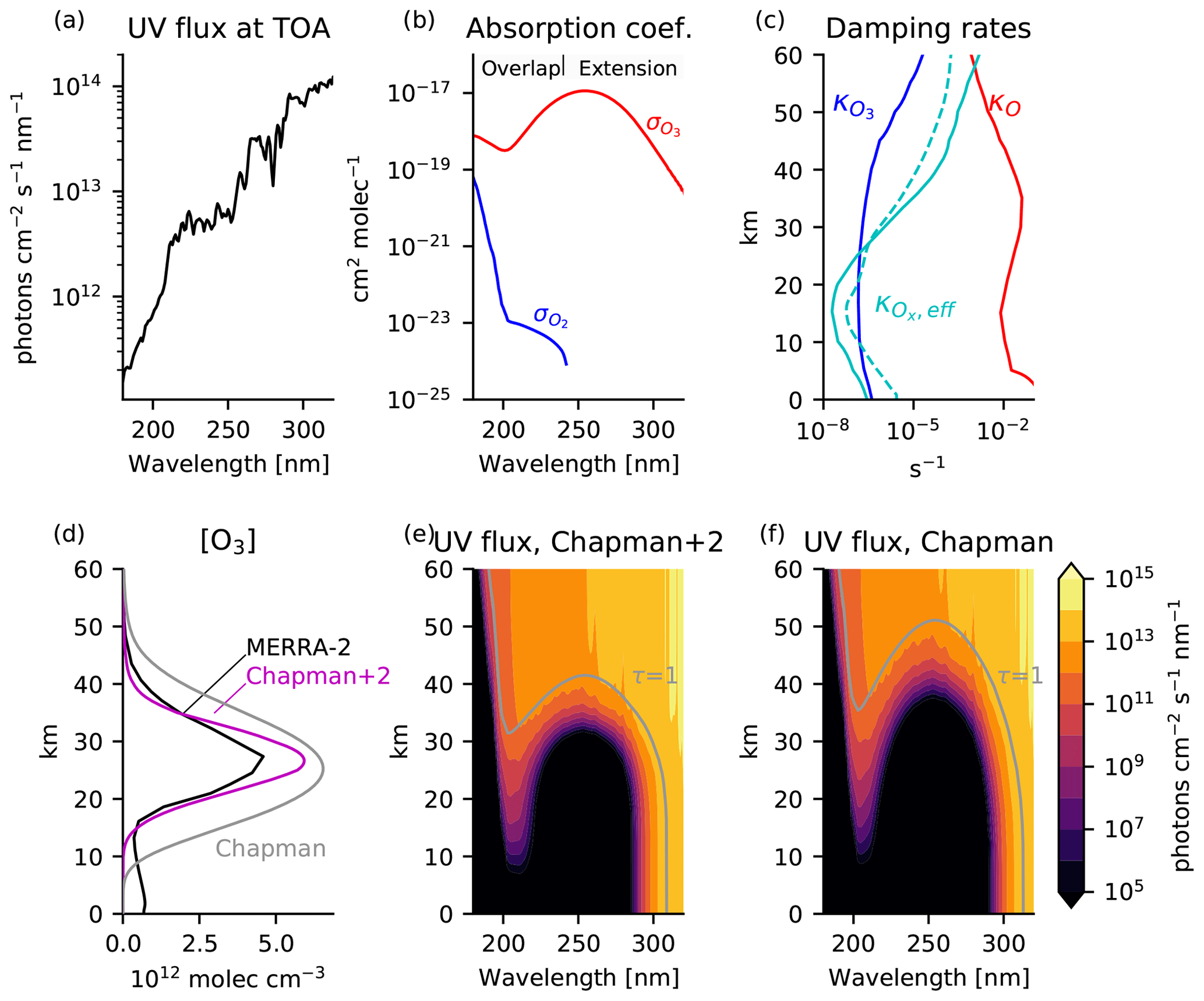
Figure 5 Boundary conditions and solutions to the Chapman+2 model. (a) UV flux at the top of the atmosphere. (b) Absorption coefficients for O₂ and O₃. (c) Generalized damping rates of O (red) and O₃ (blue) estimated from Eqs. (10) and (11), using catalyst profiles from the chemistry–climate model SOCRATES as tabulated in Brasseur and Solomon (2005). The effective damping rate of O_x (solid cyan) is comparable to the derived O₃ relaxation rate in the Cariolle v2.9 linear ozone model (dashed cyan). (d) Ozone profiles in the Chapman cycle (gray) and Chapman+2 model (magenta) compared to the O₃ profile averaged from 30° S–30° N in 2018 in the Modern Era Retrospective analysis for Research and Applications Version 2 (MERRA-2), which blends direct observations with a state-of-the-art atmosphere model to provide a state estimate of the atmosphere (black). (e) UV flux for the Chapman+2 model and (f) the Chapman cycle, indicating the level of the unit optical depth (τ(λ)=1) in gray. For clarity, wavelength axes are restricted to 180–320 nm, although the numerical solution extends up to 800 nm in the weakly absorbing Chappuis bands. An identical figure is used to introduce the Chapman+2 model in Match et al. (2024).

The Chapman+2 model equilibrium is calculated numerically, with results shown in Fig. 5. Figure 5d shows the Chapman cycle photochemical equilibrium profile of ozone (gray) compared to the Chapman+2 solution (magenta) and a tropically averaged profile in MERRA-2 for the representative year of 2018 (black) (Gelaro et al., 2017). The Chapman cycle is well-known to overestimate ozone, but this overestimate is partially mitigated in the Chapman+2 model by representing sinks from transport and catalytic cycles (Bates and Nicolet, 1950; Crutzen, 1970; Jacob, 1999; Brasseur and Solomon, 2005). Figure 5e, f show the UV flux as a function of wavelength and altitude in the equilibrium solution, with a contour indicating the τ=1 level where the UV flux at a given wavelength has been attenuated by a factor of e compared to the top-of-atmosphere UV flux.

4.3 Photochemical regimes in the Chapman+2 model

Photochemical regimes in the Chapman+2 model are calculated by first formulating the net production rate (P−L) of odd oxygen:

$$\begin{array}{}\text{(12)}& P-L=\mathrm{2}{J}_{{\text{O}}_{\mathrm{2}}}\left[{\text{O}}_{\mathrm{2}}\right]-\mathrm{2}{k}_{\mathrm{4}}\left[\text{O}\right]\left[{\text{O}}_{\mathrm{3}}\right]-{\mathit{\kappa }}_{{\text{O}}_{\mathrm{3}}}\left[{\text{O}}_{\mathrm{3}}\right]-{\mathit{\kappa }}_{\text{O}}\left[\text{O}\right].\end{array}$$

This net production rate depends on overhead column O₃ through the UV fluxes, which determine the local photolysis rates. This sensitivity of the photolysis rates to perturbations in overhead column O₃ can be calculated by differentiating Eqs. (6) and (7) with respect to ${\mathit{\chi }}_{{\text{O}}_{\mathrm{3}}}$, yielding a factor of $-{\mathit{\sigma }}_{{\text{O}}_{\mathrm{3}}}\left(\mathit{\lambda }\right)/\cos \mathit{\theta }$:

$$\begin{array}{}\text{(13)}& {\displaystyle \frac{\partial J_{{\text{O}}_{\mathrm{2}}}}{\partial {\mathit{\chi }}_{{\text{O}}_{\mathrm{3}}}}}=-\underset{\mathit{\lambda }}{\int }{q}_{O_{\mathrm{2}}}\left(\mathit{\lambda }\right){\mathit{\sigma }}_{O_{\mathrm{2}}}\left(\mathit{\lambda }\right)\stackrel{\mathrm{‾}}{I_{\mathit{\lambda }}}\left(z\right)\left({\displaystyle \frac{{\mathit{\sigma }}_{{\text{O}}_{\mathrm{3}}}\left(\mathit{\lambda }\right)}{\cos \mathit{\theta }}}\right)\mathrm{d}\mathit{\lambda },\text{(14)}& {\displaystyle \frac{\partial J_{{\text{O}}_{\mathrm{3}}}}{\partial {\mathit{\chi }}_{{\text{O}}_{\mathrm{3}}}}}=-\underset{\mathit{\lambda }}{\int }{q}_{{\text{O}}_{\mathrm{3}}}\left(\mathit{\lambda }\right){\mathit{\sigma }}_{{\text{O}}_{\mathrm{3}}}\left(\mathit{\lambda }\right)\stackrel{\mathrm{‾}}{I_{\mathit{\lambda }}}\left(z\right)\left({\displaystyle \frac{{\mathit{\sigma }}_{{\text{O}}_{\mathrm{3}}}\left(\mathit{\lambda }\right)}{\cos \mathit{\theta }}}\right)\mathrm{d}\mathit{\lambda },\end{array}$$

where $\stackrel{\mathrm{‾}}{I_{\mathit{\lambda }}}\left(z\right)$ is the basic-state UV flux. The photochemical sensitivities in Eqs. (13) and (14) are strictly negative, confirming that increasing overhead column ozone can only reduce photolysis rates by attenuating the UV flux.

The overall photochemical sensitivity of the Chapman+2 model is calculated as $\partial (P-L)/\partial {\mathit{\chi }}_{{\text{O}}_{\mathrm{3}}}$. Of course, in equilibrium the net production rate is zero, suggesting that no perturbation can modify P−L. However, the photochemical sensitivity considers a situation that is out of equilibrium, insofar as it asks the following: in response to a perturbation in the overhead column O₃ that leads to a local perturbation in UV fluxes, would the net production rate of ozone tend to increase or decrease? In other words, the photochemical sensitivity is calculated by perturbing the overhead column O₃ but keeping local ozone fixed (and therefore out of equilibrium). We calculate this photochemical sensitivity beginning with Eq. (12), substituting in the expression for atomic oxygen (Eq. 5) and then differentiating with respect to column O₃ while keeping O₃ fixed (at $\stackrel{\mathrm{‾}}{\left[{\text{O}}_{\mathrm{3}}\right]}$), yielding

$$\begin{array}{}\text{(15)}& {\displaystyle \frac{\partial (P-L)}{\partial {\mathit{\chi }}_{{\text{O}}_{\mathrm{3}}}}}=\mathrm{2}{\displaystyle \frac{\partial J_{{\text{O}}_{\mathrm{2}}}}{\partial {\mathit{\chi }}_{{\text{O}}_{\mathrm{3}}}}}\left[{\text{O}}_{\mathrm{2}}\right](\mathrm{1}-\mathit{ϵ})-\mathrm{2}\mathit{ϵ}{\displaystyle \frac{\partial J_{{\text{O}}_{\mathrm{3}}}}{\partial {\mathit{\chi }}_{{\text{O}}_{\mathrm{3}}}}}\stackrel{\mathrm{‾}}{\left[{\text{O}}_{\mathrm{3}}\right]},\text{(16)}& {\displaystyle }\mathit{ϵ}\equiv {\displaystyle \frac{k_{\mathrm{4}}\stackrel{\mathrm{‾}}{\left[{\text{O}}_{\mathrm{3}}\right]}+\frac{{\mathit{\kappa }}_{\text{O}}}{\mathrm{2}}}{k_{\mathrm{2}}{C}_{{\text{O}}_{\mathrm{2}}}{n}_{\mathrm{a}}^{\mathrm{2}}+\frac{{\mathit{\kappa }}_{\text{O}}}{\mathrm{2}}}}.\end{array}$$

The ozone layer is photochemically stabilizing when $\frac{\partial (P-L)}{\partial {\mathit{\chi }}_{{\text{O}}_{\mathrm{3}}}}<\mathrm{0}$, indicating that an increase in overhead column ozone leads to a reduction in net photochemical production. The ozone layer is photochemically destabilizing when $\frac{\partial (P-L)}{\partial {\mathit{\chi }}_{{\text{O}}_{\mathrm{3}}}}>\mathrm{0}$. When considering the photochemical sensitivity from Eq. (15), recall that $\partial J_{{\text{O}}_{\mathrm{2}}}/\partial {\mathit{\chi }}_{{\text{O}}_{\mathrm{3}}}<\mathrm{0}$ and $\partial J_{{\text{O}}_{\mathrm{3}}}/\partial {\mathit{\chi }}_{{\text{O}}_{\mathrm{3}}}<\mathrm{0}$ (Eqs. 13 and 14), because increasing overhead column O₃ reduces photolysis rates. The sensitivities of the photolytic source and sink are weighted by the leakage from the null cycle in Reaction (R2) ⇌ Reaction (R3), ϵ, which measures the strength of the photolytic sink. When ϵ is zero, there is no photolytic sink of odd oxygen, leading to strict photochemical stabilization $\left(\frac{\partial (P-L)}{\partial {\mathit{\chi }}_{{\text{O}}_{\mathrm{3}}}}<\mathrm{0}\right)$. When ϵ>0, there is a photolytic sink of odd oxygen from some combination of the Chapman sink (captured in the term $k_{\mathrm{4}}\stackrel{\mathrm{‾}}{\left[{\text{O}}_{\mathrm{3}}\right]}$) and the damping of atomic oxygen (captured in the term ${\mathit{\kappa }}_{\text{O}}/\mathrm{2}$), and photochemical destabilization becomes possible though not guaranteed. The leakage itself is small; for example, at 45 km, $\mathit{ϵ}\sim O\left({\mathrm{10}}^{-\mathrm{2}}\right)$, meaning that out of 100 photolysis events of ozone 99 will proceed into the null cycle and only 1 will leak into a sink of odd oxygen. However, photochemical destabilization nonetheless occurs at this altitude because $J_{{\text{O}}_{\mathrm{3}}}$ at 45 km is 6 orders of magnitude more sensitive to perturbations in overhead column O₃ than $J_{{\text{O}}_{\mathrm{2}}}$.

Explicit calculations of the photochemical sensitivity of the Chapman+2 model are shown in Fig. 3c. The solar zenith angle has been approximated by the latitude (neglecting the diurnal cycle) to allow a global column-by-column comparison with the photochemical sensitivity of the linear ozone models during the equinoctial month of March (Fig. 3a, b). The Chapman+2 model reproduces the gross features of the linear ozone models, most importantly the destabilizing regime above 40 km in the tropics and the stabilizing regime below. The Chapman+2 model reproduces the latitudinal dependence in which the transition between the destabilizing regime and the stabilizing regime shifts up to higher altitudes at higher latitudes. As a caveat, the representation of transport-based damping of O₃ in the Chapman+2 model is not designed to represent the extratropics, for which transport is generally a source of ozone. However, transport only enters indirectly into the photochemical sensitivity of the Chapman+2 model through its effects on the basic-state ozone, with ${\mathit{\kappa }}_{{\text{O}}_{\mathrm{3}}}$ not appearing explicitly in Eqs. (15) and (16), so these results are not expected to be overly sensitive to the unrealistic aspects of transport.

4.4 Photochemical adjustment in the Chapman+2 model

We calculate the photochemical adjustment of the Chapman+2 model in the tropical stratosphere in response to ozone depletion and cooling, considering the same perturbations as analyzed for the Cariolle v2.9 linear ozone model. It is not trivial to drive a vertically uniform loss of ozone in a fully interactive system, even one this simple, due to the vertical coupling through the UV flux. Ozone depletion is therefore imposed with an iterative calculation of ozone and overhead column ozone, working from the top of the atmosphere downwards. Starting at the uppermost level, we first compute the equilibrium [O₃] and then overwrite it with our ozone loss perturbation [O₃] − G₀. At the next level down, we can then compute the equilibrium [O₃], where the photolysis rates depend on the perturbed ozone column above. Again, this is overwritten with the imposed loss [O₃] − G₀, and the calculation proceeds iteratively downwards, yielding an ozone profile with a uniform deficit of ozone otherwise consistent with the UV flux. Stratospheric cooling is comparatively more straightforward to implement, incorporated through the temperature dependence of the collisional rates k₂ and k₄ and the generalized damping rates (Eqs. 10 and 11), using the functions for temperature dependence from Brasseur and Solomon (2005). The Chapman+2 model is designed to represent photochemistry in the stratosphere but not the troposphere, so while full profiles are shown down to the surface in order to provide a complete characterization of the stratospheric regime, these should not be regarded as representing the true response in the troposphere.

The UV-locked experiment is performed by locking both $J_{{\text{O}}_{\mathrm{2}}}$ and $J_{{\text{O}}_{\mathrm{3}}}$ to their control profiles. More refined photolysis locking is also possible in the Chapman+2 model, because we can separately lock $J_{{\text{O}}_{\mathrm{2}}}$ or $J_{{\text{O}}_{\mathrm{3}}}$. This allows us to test the prevailing explanation for the response of the ozone layer to perturbations, which neglects the sensitivity of the ozone sink ($J_{{\text{O}}_{\mathrm{3}}}$) to overhead column ozone perturbations. We perform lock sink experiments in which $J_{{\text{O}}_{\mathrm{3}}}$ is locked, quantitatively enforcing this common assumption to test whether it reproduces the fully interactive response.

The results for ozone depletion and cooling are shown in Fig. 6. These results reproduce the key structures of those from the Cariolle v2.9 linear ozone model in Fig. 4, including our two major results: (1) photochemical adjustment is destabilizing above 40 km in the tropical atmosphere and (2) photochemical adjustment is large throughout the stratosphere, with self-healing and reverse self-healing often just the tip of the iceberg.

Figure 6 The Chapman+2 model response to the same perturbations as in Fig. 4, i.e.,(a) ozone depletion by 10⁸ molec. cm⁻³ everywhere below 60 km and (b) a uniform cooling of 10 K. The Chapman+2 model reproduces the response structure calculated using the Cariolle v2.9 linear ozone model. The Chapman+2 model also permits the calculation of a lock sink response (magenta), for which only $J_{{\text{O}}_{\mathrm{3}}}$ was locked while $J_{{\text{O}}_{\mathrm{2}}}$ was allowed to adjust to the overhead ozone, emulating the conventional explanation for self-healing and reverse self-healing yet failing to reproduce key aspects of the fully interactive response.

The lock sink experiments provide a unique result from the Chapman+2 model, which could not be performed in the linear ozone model (because it did not distinguish between the photolytic source and sink). If the prevailing explanation for photochemical adjustment applied to the Chapman+2 model, then photochemical adjustment would be driven by changes in $J_{{\text{O}}_{\mathrm{2}}}$ with minimal contributions from changes in $J_{{\text{O}}_{\mathrm{3}}}$. Thus, the prevailing explanation for photochemical adjustment can be quantitatively tested by comparing the lock sink experiment (magenta) with the fully interactive experiment (black). This comparison reveals major limitations in the prevailing explanation. Because it cannot produce photochemical destabilization, the lock sink experiment fails to predict the large self-amplified destruction above 40 km in response to ozone depletion. Around 40 km in the fully interactive experiment, the contribution from self-amplified destruction actually exceeds the local magnitude of G₀, leading to absolute reductions of ozone exceeding 2G₀. At these levels of maximum self-amplified destruction, the lock sink experiment wrongly predicts photochemical stabilization. Self-healing is therefore biased towards higher altitudes in the lock sink experiment compared to in the fully interactive experiment.

Under cooling, ozone generally increases due to changes in the collisional reaction rates. This is reflected in the predicted response under UV locking (Fig. 6b, blue). Of course, these increases in ozone then induce photochemical adjustment. In both the Chapman+2 model and the Cariolle v2.9 linear ozone model, the fully interactive response of the ozone layer already deviates at high altitudes from the UV-locked response, reflecting this photochemical adjustment (Fig. 6b, red dashed curve). Photochemical adjustment generally stabilizes the ozone layer in response to cooling, although there is subtle destabilization above 40 km. Reverse self-healing, in which ozone is reduced in the fully interactive experiment compared to the control experiment (negative values of the black curve), is generally considered to be the primary manifestation of photochemical stabilization. However, reverse self-healing only captures a sliver of the much larger photochemical stabilization (negative values of the red curve). Interestingly, the lock sink calculation better reproduces the ozone response to cooling (Fig. 6b) than to depletion (Fig. 6a).

5 A spectral interpretation of photochemical stabilization and destabilization

The linear ozone models and the Chapman+2 model robustly agree on the altitude of the photochemical regime transition from destabilization aloft to stabilization below. Thus, this regime transition is likely explained by the simple physics that is shared by these models. Indeed, we find that the regime transition is controlled by which parts of the absorption spectrum for O₃ and O₂ have been attenuated versus which parts of the absorption spectrum are still active. Two key spectral windows will turn out to determine the overall photochemical regime: (1) the overlap window, which has absorption by both O₂ and O₃, occurring for λ<240 nm; and (2) the extension window, which has absorption by only O₃, occurring for λ>240 nm. These absorption spectra are shown in Fig. 5b.

The overlap window can produce either photochemical stabilization, where photons switch between being absorbed by O₂ and O₃ (e.g., Crutzen, 1974), or photochemical destabilization, where photons are absorbed by O₃ in both the control and perturbed cases. The extension window can only support photochemical destabilization, because photons must be absorbed by O₃ in both cases. Thus, the photochemical sensitivity is determined by the relative sensitivity of absorption in these two windows to perturbations in overhead column O₃. This relative sensitivity is in turn controlled by a single variable endogenous to the ozone dynamics – overhead column ozone – leading to the following photochemical regimes.

• Photochemically neutral regime. When overhead column ozone is so small that the ozone layer is optically thin at all wavelengths, absorption in both windows varies linearly with overhead column ozone, and the ozone layer is photochemically neutral.

• Photochemically destabilizing regime. As overhead column ozone increases, the first wavelength to saturate with respect to absorption by ozone (i.e., exceed ${\mathit{\tau }}_{{\text{O}}_{\mathrm{3}}}\approx \mathrm{1}$) occurs at the peak absorption coefficient of ozone of ${\mathit{\sigma }}_{{\text{O}}_{\mathrm{3}}}\approx {\mathrm{10}}^{-\mathrm{17}}$ cm² molec.⁻¹ (Fig. 6b). The unit optical depth is thus first reached for an overhead column ozone of ${\mathit{\chi }}_{{\text{O}}_{\mathrm{3}}}=\mathrm{1}/{\mathit{\sigma }}_{{\text{O}}_{\mathrm{3}},\text{max}}\approx {\mathrm{10}}^{\mathrm{17}}$ molec. cm⁻². The wavelengths where absorption first saturates are in the Hartley band centered in the extension window. Therefore, at these overhead column ozone values, absorption in the extension window is more sensitive to perturbations in overhead column ozone than is absorption in the overlap window, which remains optically unsaturated. Because absorption in the extension window is by ozone only, this means that the ozone sink is more sensitive to perturbations in overhead column ozone than the ozone source, a destabilizing regime.

• Photochemically stabilizing regime. As overhead column ozone increases further, the overlap window optically saturates around an overhead column ozone of 10¹⁸ molec. cm⁻². Beyond this overhead column ozone threshold, the ozone source in the overlap window attenuates exponentially as a function of overhead column ozone, whereas the ozone sink in the extension window still has some unsaturated wavelengths that attenuate linearly as a function of overhead column ozone. Thus, absorption in the overlap window becomes more sensitive than in the extension window, stabilizing the ozone layer.

The bottom of the destabilization layer occurs robustly around 40 km in the tropics because that is where overhead column ozone surpasses the stabilization threshold of 10¹⁸ molec. cm⁻². These overhead column ozone thresholds have been validated with mechanism denial experiments using the Chapman+2 model. For example, we flattened the absorption coefficients in the overlap window and then artificially varied them across 2 orders of magnitude. As expected, destabilization begins once the peak absorption of the Hartley band saturates and stabilization begins once the overlap window saturates, as shown in Fig. 7. Thus, if the overlap window is forced to have an absorption coefficient comparable to the peak absorption of the Hartley band, then destabilization vanishes (Fig. 7d).

Figure 7 Photochemical adjustment in the Chapman+2 model in response to uniform ozone depletion under different constant values of ${\mathit{\sigma }}_{{\text{O}}_{\mathrm{3}}}$ in the overlap window. (a) The absorption spectra where ${\mathit{\sigma }}_{{\text{O}}_{\mathrm{3}}}$ in the overlap window is flattened at various constant values. (b–d) For each constant value of ${\mathit{\sigma }}_{{\text{O}}_{\mathrm{3}}}$, (normalized) photochemical adjustment is calculated in response to a uniform ozone depletion of G₀=10⁸ molec. cm⁻³ below 60 km. Spectral theory (Sect. 5) correctly predicts that destabilization (ΔO₃<0) begins at the overhead column ozone threshold where the extension window begins to saturate (green downward-pointing triangle). Spectral theory also correctly predicts the transition from destabilization to stabilization at the overhead column ozone threshold where the overlap window saturates (upward-pointing triangles), which varies across the three experiments. If the top and bottom of the destabilization regime occur at the same altitude, then the destabilization regime vanishes (d). Photochemical adjustment using the true absorption coefficients is plotted as the red dashed curve (identical in panels b–d and as plotted in Fig. 6a).

The principle that destabilization occurs where the overlap window is optically unsaturated has been validated in the Cariolle v2.9 and LINOZ linear ozone models. Figure 3 includes magenta curves corresponding to the slant overhead column ozone threshold of 10¹⁸ molec. cm⁻², where slant overhead column ozone has been calculated as ${\mathit{\chi }}_{{\text{O}}_{\mathrm{3}}}/\cos \left(\mathit{\theta }\right)$, with θ taken as the latitude (noting that we chose an equinoctial month to approximately equate latitude with zenith angle while neglecting the diurnal cycle in the Sun angle). In the linear ozone models, the climatological overhead column ozone is given by the parameter A₇, and in the Chapman+2 model the climatological ozone is calculated at each latitude, approximating θ with latitude. Although imperfect, the theoretical curve approximately reproduces the transition from destabilization to stabilization, including its latitudinal structure (Fig. 3). At high latitudes, the transition from destabilization to stabilization occurs at a higher altitude due to the oblique angle of the sunlight, which reaches the slant overhead column ozone threshold more rapidly for a given ozone profile.

6 Updating the explanation for self-healing and reverse self-healing

Photochemical models produce photochemical adjustment as a natural consequence of accurately representing photochemistry. Thus, the key results of this paper are primarily conceptual, since they inform how the sensitivity of the ozone layer to perturbations is interpreted and explained. These results could also have implications for certain decisions made when formulating photochemical models, which is considered in the Discussion section. However, the main conceptual advances from this paper suggest that some of the previous explanations of ozone self-healing and reverse self-healing could distort understanding of photochemical adjustment.

Most explanations suggest that self-healing and reverse self-healing can be understood by considering the effect of the perturbed ultraviolet fluxes on the photolytic ozone source. For example, self-healing is explained in Hudson (1977) as follows: “O₃ destruction at the upper levels in the stratosphere is partially compensated by the increase in O₃ at the lower levels due to deeper penetration of solar UV radiation.” Similarly, in one of the few textbook explanations of self-healing, Finlayson-Pitts and Pitts (2000) wrote that “When stratospheric O₃ is removed ... there is more light available for photolysis of O₂ and the formation of more ozone.” Although not strictly wrong, these explanations might lead to the incorrect impression that deeper penetration of solar UV radiation generally leads to increased ozone. Instead, we have shown that this common explanation only gives correct intuition for the stabilizing regime of ozone photochemistry but not the destabilizing regime. Photochemical adjustment cannot generally be understood by only considering the effects of the perturbation ultraviolet flux on the ozone source. Neglecting the effects of the perturbation ultraviolet flux on the ozone sink was shown to lead to errors in the magnitude and vertical structure of the photochemical adjustment (Fig. 6).

Thus, it seems plausible to formulate a minimal explanation for self-healing and reverse self-healing as follows:

• Self-healing. Ozone depletion enhances ultraviolet fluxes penetrating to lower altitudes, increasing both the ozone source and the ozone sink. Ozone exhibits a local net increase (self-healing) if the photolytic ozone source increases more than the photolytic ozone sink and that increase is large enough to overcome any local ozone depletion.

• Reverse self-healing. Ozone enhancement reduces ultraviolet fluxes penetrating to lower altitudes, reducing both the ozone source and the ozone sink. Ozone exhibits a local net decrease (reverse self-healing) if the photolytic ozone source decreases more than the photolytic ozone sink and that decrease is large enough to overcome any local ozone enhancement.

7 Discussion

7.1 Sink regimes of the Chapman+2 model

The photolytic sink of O₃, resulting from leakage out of the null cycle Reaction (R2) ⇌ Reaction (R3), is in some places the dominant sink of O₃, but this is not dominant everywhere. Where the photolytic sink is not the dominant sink of O₃, modulation of the photolytic sink by photochemical adjustment is not expected to be as significant in determining O₃. Match et al. (2024) analyzed limiting cases of the Chapman+2 model in which each of its three sinks of odd oxygen dominates: the Chapman cycle sink limit (Reaction R4), the O-damped limit (Reaction R5), and the O₃-damped limit (Reaction R6). When these limits are strictly satisfied and under other realistic assumptions such as O₃ being the dominant absorber of UV, these limits lead to the following distinct scaling relationships for the ozone profile with altitude:

$$\begin{array}{}\text{(17)}& {\displaystyle }[{\text{O}}_{\mathrm{3}}{]}_{\text{Chapman}}={\left({\displaystyle \frac{J_{{\text{O}}_{\mathrm{2}}}{k}_{\mathrm{2}}}{J_{{\text{O}}_{\mathrm{3}}}{k}_{\mathrm{4}}}}\right)}^{\mathrm{1}/\mathrm{2}}{C}_{{\text{O}}_{\mathrm{2}}}{n}_{\mathrm{a}}^{\mathrm{3}/\mathrm{2}},\text{(18)}& {\displaystyle }[{\text{O}}_{\mathrm{3}}{]}_{\text{O-damped}}={\displaystyle \frac{\mathrm{2}{J}_{{\text{O}}_{\mathrm{2}}}{k}_{\mathrm{2}}{C}_{{\text{O}}_{\mathrm{2}}}^{\mathrm{2}}{n}_{\mathrm{a}}^{\mathrm{3}}}{J_{{\text{O}}_{\mathrm{3}}}{\mathit{\kappa }}_{\text{O}}}},\text{(19)}& {\displaystyle }[{\text{O}}_{\mathrm{3}}{]}_{{\mathrm{O}}_{\mathrm{3}}\text{-damped}}={\displaystyle \frac{\mathrm{2}{J}_{{\text{O}}_{\mathrm{2}}}{C}_{{\text{O}}_{\mathrm{2}}}{n}_{\mathrm{a}}}{{\mathit{\kappa }}_{{\text{O}}_{\mathrm{3}}}}}.\end{array}$$

Analyzing the tropical stratosphere in the Chapman+2 model, Match et al. (2024) demonstrated that the ozone layer can be approximated as being in an O-damped limit above 26 km (i.e., above the peak in [O₃]). The O-damped limit results from catalytic destruction of atomic oxygen, most importantly by the NO_x cycle. The atomic oxygen that is being catalytically damped in the O-damped limit must be liberated through photolysis of O₃, so the O-damped limit has a photolytic sink of O₃. The suppression of O₃ by photolysis of O₃ is evident by $J_{{\text{O}}_{\mathrm{3}}}$ appearing in the denominator of the O-damped limit (Eq. 18). In the photolytic sink regime, photochemical adjustment can be either stabilizing or destabilizing, depending on whether $J_{{\text{O}}_{\mathrm{2}}}$ or $J_{{\text{O}}_{\mathrm{3}}}$ is more strongly affected (fractionally) by the overhead perturbation.

Below 26 km (i.e., below the peak in [O₃]), the stratospheric ozone layer can be approximated as being in an O₃-damped limit. The damping of O₃ arises primarily from transport, which dilutes ozone in the tropical lower stratosphere by upwelling ozone-poor air from below. When the dominant sink of odd oxygen is from damping of O₃, the photolytic sink of O₃ no longer dictates the structure. This can be seen in the absence of $J_{{\text{O}}_{\mathrm{3}}}$ from Eq. (19). With this non-photolytic sink, only perturbations to $J_{{\text{O}}_{\mathrm{2}}}$ matter, and photochemical adjustment must be stabilizing. Thus, conventional explanations for self-healing and reverse self-healing are strictly true in the O₃-damped limit and therefore capture the leading-order response to perturbations in the tropical lower stratosphere.

The O-damped limit and the Chapman cycle both have a photolytic sink of O₃, and both produce ozone that scales as $(J_{{\text{O}}_{\mathrm{2}}}/J_{{\text{O}}_{\mathrm{3}}}{)}^n$ (n=1 for the O-damped limit and $n=\mathrm{1}/\mathrm{2}$ for the Chapman cycle) (Match et al., 2024). The photolytic sink of the O-damped limit arises because catalytic damping of atomic oxygen is rate-limited in atomic oxygen, whereas the photolytic sink of the Chapman cycle arises because Reaction (R4) is limited by the availability of atomic oxygen produced by photolysis of O₃. That the Chapman cycle also has a photolytic sink means that it reproduces key photochemical sensitivities from the more realistic O-damped limit. This helps explain why Hartmann (1978), who analyzed a version of the Chapman cycle that did not include explicit catalytic sinks or transport, nonetheless found photochemical destabilization at the correct altitude above 40 km in their tropical profile.

It has been suggested that self-healing and reverse self-healing are damped by transport, i.e., that photochemistry would stabilize a larger fraction of the UV anomaly if not for the damping effects of transport (Solomon et al., 1985). The fraction of photochemical stabilization is important because, in a hypothetical world with perfect photochemical stabilization, ozone-depleting substances that destroy ozone aloft would add exactly the same amount of ozone back through self-healing, eliminating anthropogenic impacts on the ozone layer. Thus, it is only the observed deviations below perfect stabilization that cause risks from ozone-depleting substances and benefits from their mitigation.

Does transport suppress the fraction of photochemical stabilization, as has been argued, by damping O₃ anomalies in the lower stratosphere? The answer is not clear-cut when the basic-state effects of the transport are accounted for, because although O₃ damping by transport certainly damps O₃, it also creates the O₃-damped regime of the lower stratosphere that is prone to photochemical stabilization. Transport introduces the possibility that O₃ depletion aloft can allow more ultraviolet fluxes below that speed up photochemical equilibration in the lower stratosphere, shifting down the transition altitude between the O₃-damped limit and the O-damped limit. Reflecting this nuance, increasing ${\mathit{\kappa }}_{{\text{O}}_{\mathrm{3}}}$ in the Chapman+2 model actually increases the fractional stabilization of the UV-locked O₃ anomaly from stratospheric cooling while reducing the fractional stabilization of the UV-locked O₃ anomaly from O₃ depletion. Further work could clarify whether transport amplifies or suppresses this fraction of photochemical stabilization.

7.2 Photochemical destabilization is not an instability

Photochemical adjustment does not involve feedback; i.e., perturbations in overhead column O₃ affect O₃ below a given altitude, but they do not affect O₃ at that altitude. The effects of photochemical adjustment cascade downwards through the column. In the absence of a local feedback, photochemical destabilization cannot lead to a local photochemical instability in which ozone anomalies run away to become arbitrarily large or small. Photochemical adjustment is analogous to a snowball rolling down a hill, which grows in proportion to itself in regions of destabilization and shrinks in proportion to itself in regions of stabilization. This analogy provides intuition for two key aspects of photochemical adjustment: (1) there is no local feedback (the snowball cannot grow while remaining stationary), and (2) the peak photochemical anomalies are set by the magnitude of destabilization and the depth of the atmosphere (length of the hill).

7.3 Implications

The concepts of photochemical stabilization and destabilization explain major features of chemistry–climate model simulations that coexisted uneasily with previous theory. Nonetheless, this work also has methodological and physical implications that extend beyond understanding pre-existing model phenomena.

A methodological implication of this work can be found in the construction of linear ozone models. In McCormack et al. (2006), a linear ozone model is formulated based on the CHEM2D model. In calculating the coefficients for the sensitivity to overhead column ozone perturbations, they encoded into their method the assumption that photolysis of ozone does not contribute to the destruction of ozone. Thus, they calibrated their sensitivities to perturbations in overhead column ozone based only on the effects of changes in the photolytic source of ozone. This approach appears to forbid photochemical destabilization by construction. Their approach is equivalent to our lock sink calculation in Fig. 6, which was shown to induce large biases compared to a fully interactive calculation, especially in response to ozone depletion.

A physical implication of this work is that, because photochemical destabilization occurs below a threshold of overhead column ozone of roughly 10¹⁸ molec. cm⁻², atmospheres with less ozone could have deeper regions of photochemical destabilization. In today's tropical atmosphere, destabilization occurs above 40 km, encompassing approximately 4 % of the ozone layer. This overhead column ozone threshold would occur at a much lower altitude and could encompass a much larger fraction of the ozone layer in an atmosphere with less total ozone. The atmosphere had lower ozone throughout much of Earth's history, over which atmospheric O₂ has increased by 7 orders of magnitude, and overhead column ozone has correspondingly increased from being vanishingly small to its present values (Kasting and Donahue, 1980). If ozone increased continuously, then there must have been an era when the total column ozone was approximately 10¹⁸ molec. cm⁻², during which our theory predicts that the ozone layer could have been completely photochemically destabilizing. This could have amplified the effects of processes that add or deplete ozone, thereby amplifying the variability of UV light reaching the surface and affecting early life. Similarly, planets outside our solar system could have ozone layers that are photochemically destabilizing. Ozone layers at varying concentrations of O₂ have been simulated using one-dimensional models (Kasting and Donahue, 1980; Levine, 1977; Segura et al., 2003) and, recently, chemistry–climate models (Cooke et al., 2022; Józefiak et al., 2023), but the photochemical sensitivity of the ozone layer has not been quantified for atmospheres with different amounts of O₂, which is a subject for future work.

8 Conclusions

It has long been known that the photochemical nature of the ozone layer causes it to respond counterintuitively to perturbations. Ozone-depleting substances can lead to increases in ozone at some altitudes (known as self-healing), which have been argued to result from ultraviolet fluxes reaching deeper into the atmosphere. Processes that increase ozone, such as stratospheric cooling, can lead to decreases in ozone below (known as reverse self-healing), which have been argued as resulting from the decreased ultraviolet fluxes reaching lower altitudes. We have pursued a quantitative characterization and understanding of the photochemical processes that lead to self-healing and reverse self-healing. To do so, we have defined photochemical adjustment as the component of the ozone response to a perturbation that results from changes in photolysis due to changes in overhead column ozone. Photochemical adjustment is quantified as the difference in the ozone response to a perturbation in a fully interactive photochemical experiment versus with UV fluxes locked to their unperturbed values.

Photochemical sensitivities were quantified in two linear ozone models: Cariolle v2.9 and LINOZ. Photochemical adjustment was further quantified in column calculations using Cariolle v2.9 for the response to ozone depletion and stratospheric cooling. Photochemical adjustment can be stabilizing, damping overhead column ozone perturbations towards the surface and potentially leading to self-healing and reverse self-healing. Self-healing and reverse self-healing only occur for the subset of photochemical stabilization in which the photochemical adjustment dominates the local effects of the perturbation, making them just the tip of the iceberg for often large photochemical adjustment. We have also characterized a new and unconventional region of photochemical destabilization above 40 km in the tropical stratosphere and even farther aloft at high latitudes.

The regimes of photochemical stabilization and destabilization in the linear ozone models (Cariolle v2.9 and LINOZ) were successfully emulated using a Chapman+2 model of the ozone layer, which augments the Chapman cycle with generalized destruction of O and O₃ by catalytic cycles and transport. A column-by-column calculation using the Chapman+2 model reproduces the full latitudinal structure of the transition from destabilization to stabilization (Fig. 3). Photochemical destabilization in the Chapman+2 model arises when the photolytic sink of ozone (absorption by O₃) is more sensitive than the photolytic source (absorption by O₂) to perturbations in overhead O₃. The sensitivity of the photolytic source and sink can in turn be related directly to the absorption spectra of O₂ and O₃. Photochemical destabilization occurs when absorption in the extension window (λ>240 nm) becomes optically saturated (${\mathit{\tau }}_{{\text{O}}_{\mathrm{3}}}=\mathrm{1}$) while absorption in the overlap window (λ<240 nm) remains unsaturated. Photochemical stabilization occurs once absorption by O₃ in the overlap window saturates. This spectral intuition leads to a simple theory that photochemical destabilization should occur below a threshold of slant overhead column ozone of approximately 10¹⁸ molec. cm⁻², which reproduces the latitudinal structure of the transition altitude between destabilization and stabilization in the linear ozone models and the Chapman+2 model.

Roughly 4 % of ozone molecules in the tropics today are in a photochemically destabilizing regime. As considered in the Discussion section as a subject for future work, an atmosphere with less total ozone will have a higher fraction of its ozone layer in a destabilizing regime below the overhead column ozone threshold of 10¹⁸ molec. cm⁻². Over Earth's history, atmospheric O₂ has increased by at least 7 orders of magnitude, leading to the formation of the ozone layer (e.g., Kasting and Donahue, 1980). Paleoclimatic ozone layers with total column ozone below the destabilization threshold could have been completely destabilizing, amplifying ozone perturbations and increasing the variability of the UV light experienced by early life.