Trends in the high-latitude mesosphere temperature and mesopause revealed by SABER

The temperature trend in the mesosphere and lower-thermosphere (MLT) region can be regarded as an indicator of climate change. Using temperature profiles measured by the Sounding of the Atmosphere using Broadband Emission Radiometry (SABER) instrument during 2002–2023 and binning them based on the yaw cycle, we obtain a continuous dataset with a wide local time coverage at 50° S–80° N or 80° S–50° N. The seasonal change in temperature, caused by the forward drift in the SABER yaw cycle, is removed using the climatological temperature of the Naval Research Laboratory's Mass Spectrometer Incoherent Scatter Radar model (MSIS2.0). The corrected temperature without any waves is regarded as the mean temperature. At 50° S–50° N, the cooling trends in the mean temperature are significant in the MLT region and are in agreement with previous studies. The novel finding is that the cooling trends of ≥ l2 K per decade exhibit seasonal symmetry and reach peaks of ≥ 6 K per decade at high latitudes around the summer solstice. Moreover, there are warming trends of 1–2.5 K per decade at an altitude range of 10⁻²–10⁻³ hPa, specifically at latitudes higher than 55° N in October and December and at latitudes higher than 55° S in April and August. Over the past 22 years, the mesopause temperature (altitude) in the northern summer polar region has been ∼ 5–11 K (∼ 1 km) colder (lower) than that in the corresponding southern region. The trends in the mesopause temperature are dependent on latitudes and months, but they are negative at most latitudes and reach larger magnitudes at high latitudes. These results indicate that the temperature in the high-latitude MLT region is more sensitive to dynamic changes.

1 Introduction

Observational and simulation studies have revealed that the global-mean temperature trend is cooling in the mesosphere and lower thermosphere (MLT) (Beig et al., 2003; Laštovička et al., 2006; Yue et al., 2019b; Laštovička, 2023). The cooling trends observed in the MLT region are mainly caused by increases in anthropogenic greenhouse gases, such as carbon dioxide. Moreover, changes in the stratospheric ozone depletion and recovery, increasing mesospheric water vapor concentration, and solar and geomagnetic variations may also contribute to long-term changes in temperature in the MLT region (Laštovička, 2009; Yue et al., 2019a, 2015; Garcia et al., 2019; Mlynczak et al., 2022; Zhang et al., 2023).

A recent review work by Laštovička (2023) summarized that temperature trends are generally cooling but that they also depend on local times, heights, and geographic locations in the MLT region (Venkat Ratnam et al., 2019; Das, 2021; She et al., 2019; Yuan et al., 2019; Ramesh et al., 2020). These results were mostly derived from ground-based and satellite observations at low and middle latitudes, while the simulations provided insights into the long-term trends from pole to pole. On the other hand, due to scarce observations, the long-term trends in temperature at high latitudes have not been thoroughly examined and are not yet well understood. Driven by the summer-to-winter meridional circulation, the upwelling causes adiabatic cooling in the summer polar mesosphere, while the downwelling causes adiabatic warming in the winter polar mesosphere (Dunkerton, 1978; Garcia and Solomon, 1985). Thus, the high-latitude temperature is more sensitive to changes in the dynamics, wave forcing, stratospheric wind, etc. (Russell et al., 2009; Qian et al., 2017; Yu et al., 2023).

The progress in studying long-term trends in the MLT region has been summarized and reported by Laštovička and Jelínek (2019) and Laštovička (2023). Here, we highlight some studies related to the temperature trends at high latitudes. Using temperature measured by the Sounding of the Atmosphere using Broadband Emission Radiometry (SABER) instrument and simulated by version 4 of the Whole Atmosphere Community Climate Model (WACCM4), Garcia et al. (2019) showed that the global-mean SABER temperature (52° S–52° N) had cooling trends of 0.4–0.5 K per decade during 2002–2018 in the stratosphere and mesosphere. These magnitudes were smaller than those simulated by WACCM4 (0.6–0.9 K per decade) but within 2 times the standard deviation. Using the Leibniz Institute Middle Atmosphere Model (LIMA) under Northern Hemisphere (NH) conditions during 1871–2008, Lübken et al. (2018) showed that the cooling trend in the MLT region was 1.5 K per decade during 1960–2008, while it was 0.7 K per decade during 1871–2008 at 55–61° N for geometric heights. However, the trend was neglectable for pressure heights. For pressure heights, the global-mean SABER temperature (55° S–55° N) had cooling trends of 0.5 and 2.6 K per decade at 10⁻³ hPa (∼ 92 km) and 10⁻⁴ hPa (∼ 106 km), respectively, during 2002–2021 (Mlynczak et al., 2022). The results of Lübken et al. (2018) and Mlynczak et al. (2022) illustrated that the cooling trends were larger over recent decades for both geometric and pressure heights compared with the beginning of industrialization. To achieve a longer time series, Li et al. (2021) constructed a nearly 30-year dataset at 45° S–45° N by merging the temperature measured by the Halogen Occultation Experiment (HALOE) instrument during 1991–2005 and the SABER instrument during 2002–2019. They showed that the cooling trend was significant and reached a peak of 1.2 K per decade at 60–70 km in the Southern Hemisphere (SH) tropical and subtropical regions. Moreover, the cooling trend in the SH was larger than its counterpart in the NH.

At high latitudes, ground-based observations of OH nightglow rotational temperature revealed a significant cooling trend of 1.2 ± 0.51 K per decade at Davis (68° S, 78° E) during 1995–2019 (French et al., 2020). The OH rotational temperature around midnight exhibited a significant cooling trend of 2.4 ± 2.3 K per decade in summer and an insignificant cooling trend of 0.4 ± 2.2 K per decade in winter in Moscow (57° N, 37° E) during 2000–2018 (Dalin et al., 2020). Using the ice layer parameters simulated by the LIMA model and the Mesospheric Ice Microphysics And tranSport (MIMAS) ice particle model, Lübken et al. (2021) showed that the negative trend in noctilucent cloud altitudes (∼ 83 km) was primarily caused by increasing CO₂ in the troposphere at 58° N, 69° N, and 78° N during 1871–2008. At these three latitudes, the cooling trends were ∼ 0.2 K per decade during 1871–1960 and 1.0 K per decade during 1960–2008. Near the latitude band of 64–70° N in June and 64–70° S in December, Bailey et al. (2021) constructed two datasets by merging the temperature measured by HALOE and SABER and by HALOE and SOFIE (Solar Occultation for Ice Experiment). They showed that there were cooling trends of ∼ 1–2 K per decade near 0.1–0.01 hPa (∼ 68–80 km) and warming trends of ∼ 1 K per decade near 0.005 hPa (∼ 85 km) at 64–70° N in June and 64–70° S in December. Moreover, the WACCM-X simulation results by Qian et al. (2019) showed that the temperature trends were mostly cooling in the MLT region. However, there was also warming at ∼ 80–95 km in the SH polar region from November to February (Fig. 3 of Qian et al., 2019). The disagreement in these results at high latitudes might be attributed to the different temporal spans and local times, observations using different instruments, and different methods for deriving the trends. Thus, there is an urgent need to study the temperature trends at high latitudes using one coherent measurement over a long period.

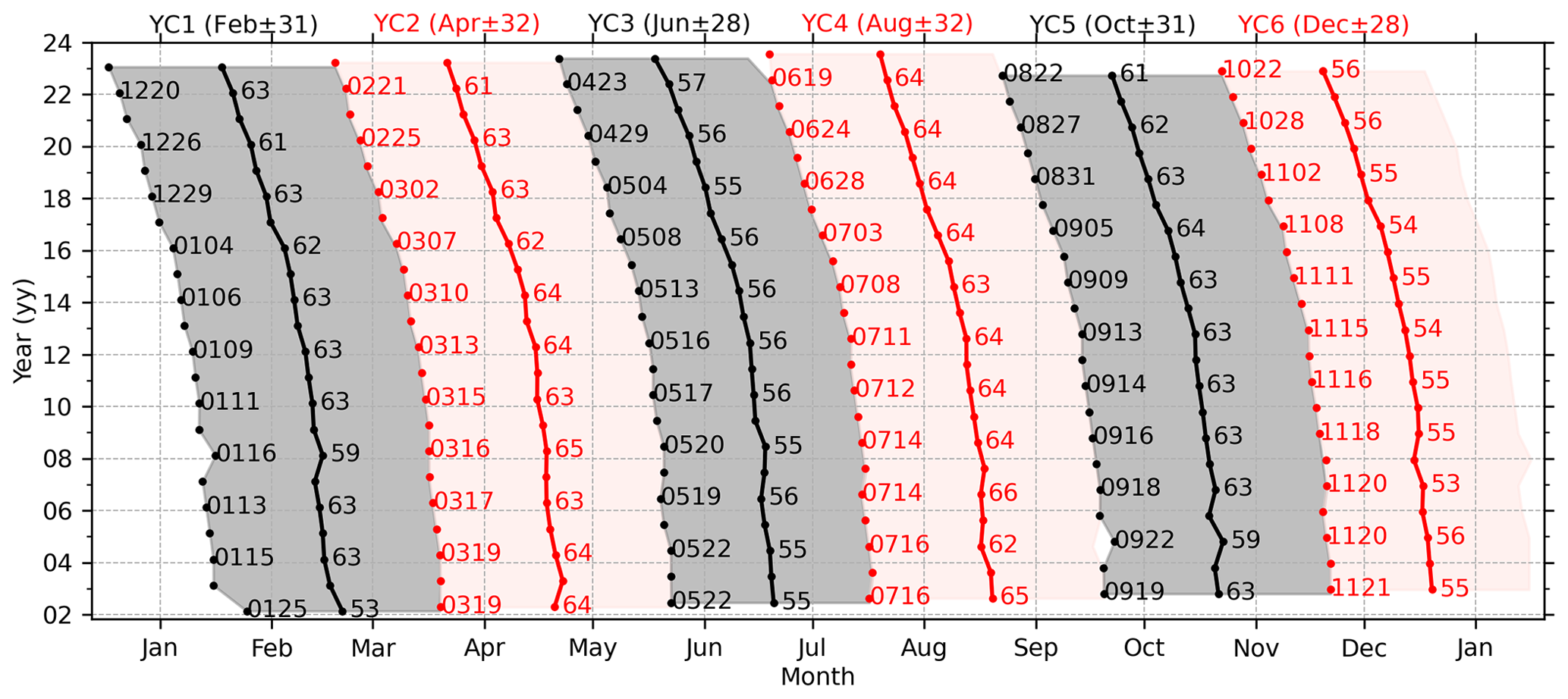
Figure 1 The temporal span of each yaw cycle (YC) from 2002 to 2023. The gray (red) region indicates the northward-viewing (southward-viewing) maneuver. The beginning date (“mmdd” format, where “mm” and “dd” denote the month and the day of the month, respectively) and temporal span (in days) of each yaw are labeled on the right of the beginning date (dots) and center date (line with dots), respectively. The six YCs and their center date in 2003 as well as their half-spans are labeled as YC1–YC6 at the top of the panel and also listed in Table 1.

The SABER temperature profiles cover latitudes of 53° S–83° N in the northward-viewing maneuvers and 83° S–53° N in the southward-viewing maneuvers beginning in 2002. The SABER operational temperature profile covers an altitude range of ∼ 15–110 km. The precision and systematic error in the SABER temperature profile are height dependent. For a single temperature profile, the precision values are summarized at https://spdf.gsfc.nasa.gov/pub/data/timed/saber/ (last access: 31 January 2024) and are 1.8 K at 80 km, 3.6 K at 90 km, 6.7 K at 100 km, and 15.0 K at 110 km at a vertical resolution of 2 km. Moreover, for a single temperature profile, the systematic errors defined by 1 standard deviation (corresponding to a confidence level of 68 %) are ∼ 1.4 K at and below 80 km, 4.0 K at 90 km, 5.0 K at 100 km, and 25.0 K at 110 km for typical midlatitude conditions (Remsberg et al., 2008; Rezac et al., 2015; Dawkins et al., 2018). The systematic errors will be doubled if they are defined by 2 times the standard deviation (corresponding to a confidence level of 95 %). These data have exhibited remarkable stability over the last 2 decades, following the correction of algorithm instability (Mlynczak et al., 2020, 2022, 2023). Using the SABER temperature profiles during 2002–2019, Zhao et al. (2020) employed a 60 d moving window to obtain the mean temperature. Their analysis revealed that the annual and global-mean trend in the mesopause temperature is cooling at a magnitude of 0.75 K per decade. Moreover, the cooling trend is significant in non-summer seasons but insignificant in summer (May–August) at 60–80° N/S. It should be noted that the SABER yaw cycle (YC) drifted forward about 1 month from 2002 to 2023 (see Fig. 1) due to a changing satellite orbit. As a result, the local time (LT) coverage in a certain month differs from year to year at high latitudes if the window is constantly set to be 60 d.

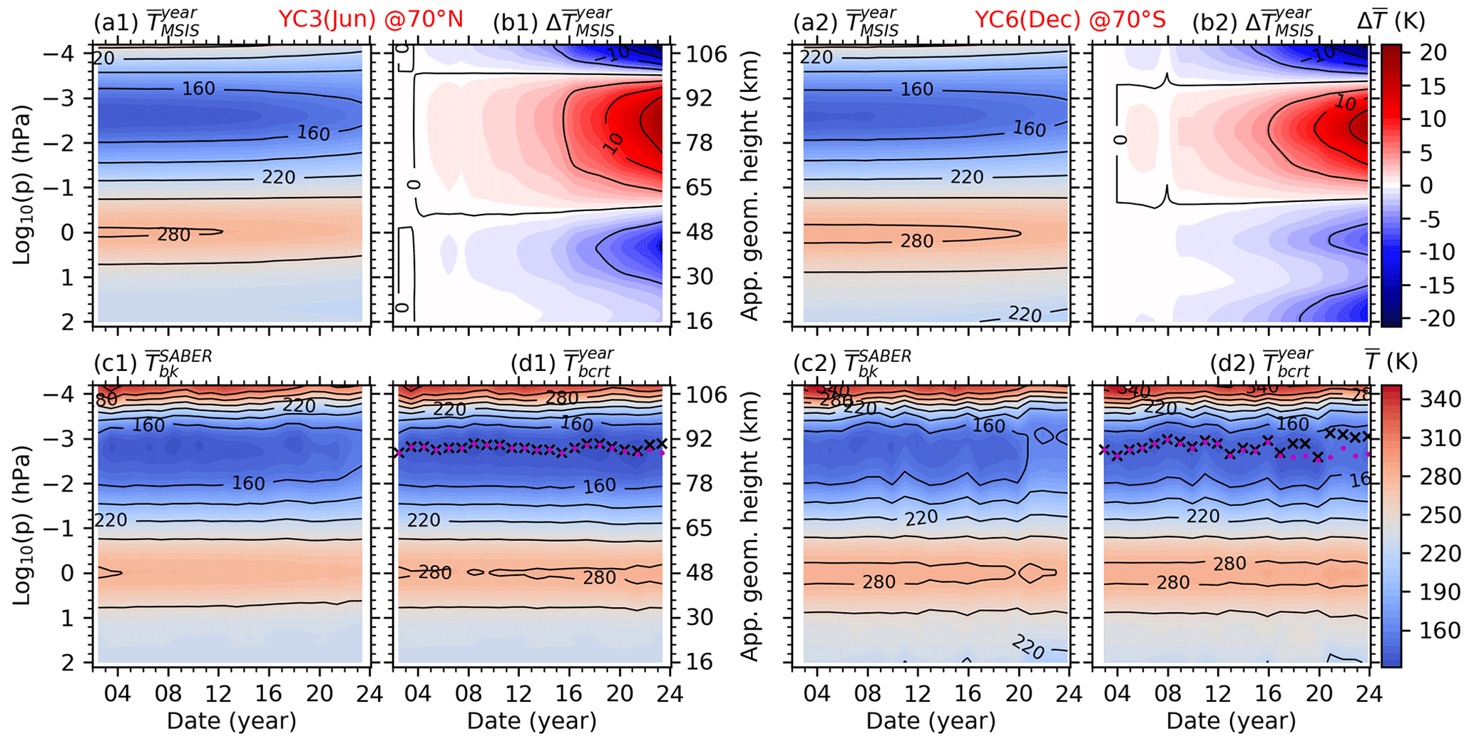
Figure 2 The date–height distributions of the mean temperature calculated from NRLMSIS 2.0 (${\stackrel{\mathrm{‾}}{T}}_{\text{MSIS}}^{\text{year}}$) and SABER (${\stackrel{\mathrm{‾}}{T}}_{\text{bk}}^{\text{year}}$) at 70° N in YC3 (left two columns) and at 70° S in YC6 (right two columns). ${\stackrel{\mathrm{‾}}{T}}_{\text{MSIS}}^{\text{year}}$ is used as a reference to calculate the seasonal variation ($\mathrm{\Delta }{\stackrel{\mathrm{‾}}{T}}_{\text{MSIS}}^{\text{year}}$) caused by the forward drift in the YC from 2002 to 2023. Then, the corrected mean temperature (${\stackrel{\mathrm{‾}}{T}}_{\text{bcrt}}^{\text{year}}$) is calculated by removing $\mathrm{\Delta }{\stackrel{\mathrm{‾}}{T}}_{\text{MSIS}}^{\text{year}}$ from ${\stackrel{\mathrm{‾}}{T}}_{\text{bk}}^{\text{year}}$. The mesopause altitudes calculated from ${\stackrel{\mathrm{‾}}{T}}_{\text{bk}}^{\text{year}}$ and ${\stackrel{\mathrm{‾}}{T}}_{\text{bcrt}}^{\text{year}}$ are plotted as black crosses and red dots, respectively. The plots of ${\stackrel{\mathrm{‾}}{T}}_{\text{MSIS}}^{\text{year}}$, ${\stackrel{\mathrm{‾}}{T}}_{\text{bk}}^{\text{year}}$, and ${\stackrel{\mathrm{‾}}{T}}_{\text{bcrt}}^{\text{year}}$ have the same color bar for $\stackrel{\mathrm{‾}}{T}$. The plot of $\mathrm{\Delta }{\stackrel{\mathrm{‾}}{T}}_{\text{MSIS}}^{\text{year}}$ has the color bar of $\mathrm{\Delta }\stackrel{\mathrm{‾}}{T}$. The same y-axis scales are used in all panels. The approximate geometric height is label on the right side of the second column.

Here, we focus on the trend in the mean temperature without any atmospheric waves (i.e., gravity waves, tides or planetary waves). Calculating the zonal mean can remove gravity waves, nonmigrating tides, and long-period planetary waves. However, migrating tides depend on the LT and are strong in the MLT region. They cannot simply be removed by calculating the zonal mean. In this work, we bin the data based on the YC, which covers an interval of 54–64 d (see Fig. 1) and provides almost full LT coverage (except for the 1–3 h around noon). Thus, the mean temperature can be accurately determined by removing the migrating tides at 53° S–83° N or 83° S–53° N using harmonic fitting. Each YC in every year covers varying ranges of dates. This results in the aliasing of the seasonal variation in the temperature into the mean temperature of each YC. This issue can be resolved as outlined in the following. We use the temperature of the Naval Research Laboratory’s recently released whole-atmosphere empirical Mass Spectrometer Incoherent Scatter Radar model (MSIS2.0; Emmert et al., 2021) as a reference for the seasonal variation. This seasonal variation (more than 10 K, as seen in Fig. 2b) embedded in the YC drift is removed from the mean temperature of each YC. Thus, using the advantages of SABER measurements at high latitudes and binning the data based on YC, we focus on the long-term trends in the mean temperature and the mesopause in the high-latitude MLT region.

2 Method of calculating mean temperature and trend

The mean temperature (${\stackrel{\mathrm{‾}}{T}}_{\text{bk}}$) excludes gravity waves, tides, and planetary waves. Moreover, compared with the magnitudes of ${\stackrel{\mathrm{‾}}{T}}_{\text{bk}}$, its trend is a small value and should be determined with extra caution. The method of calculating ${\stackrel{\mathrm{‾}}{T}}_{\text{bk}}$ is based on a YC window. This ensures a good LT coverage at high latitudes. Compared with the fixed 60 d window, the advantage and necessity of the YC window are described in the following.

The YC window is defined as the temporal interval during which the SABER measurements are in the northward- or southward-viewing maneuver. Figure 1 shows the beginning date and temporal span of each YC. We see that there are about six YCs in each year, referred to as YC1–YC6. The temporal spans of YCs are 54–64 d. This ensures that the LT coverage of SABER measurements is more than 18 h at high latitudes. Therefore, migrating tides can be removed efficiently through harmonic fitting. In contrast, the LT coverage in a fixed 60 d window is different from year to year at high latitudes. This is because the temporal span of each YC drifted forward about 1 month from 2002 to 2023 (Fig. 1). For the case of the fixed 60 d window at 70° N in March (spanning from 14 February to 14 April with a center on 15 March), the sampling hours were distributed at 00:00–02:00, 05:00–11:00, and 21:00–24:00 LT and had a coverage of only 14 h in 2005. However, the sampling hours in 2022 were distributed at 00:00–10:00 and 13:00–24:00 LT and had a coverage of 22 h. The year-to-year variations in the LT distribution and coverage might induce uncertainties and biases into ${\stackrel{\mathrm{‾}}{T}}_{\text{bk}}$. Thus, the YC-dependent window is necessary to obtain a wide LT coverage.

We note that the forward drift in the YC raises the issue that each YC in every year covers varying ranges of dates. This propagates the distortion in the seasonal variation in the temperature into ${\stackrel{\mathrm{‾}}{T}}_{\text{bk}}$ and should be removed to get a corrected mean temperature (${\stackrel{\mathrm{‾}}{T}}_{\text{bcrt}}$). The detailed procedure for calculating ${\stackrel{\mathrm{‾}}{T}}_{\text{bcrt}}$ and its trend is presented in Sects. 2.1–2.3. The procedure for calculating the mesopause temperature and height is presented in Sect. 2.4.

2.1 Removing waves from SABER temperature

For each YC, the background temperature is calculated using three steps. Firstly, at each latitude band and pressure level, the daily zonal mean temperature (${\stackrel{\mathrm{‾}}{T}}_{\mathrm{d}}$) is calculated by averaging the temperature profiles at the ascending and descending nodes, respectively. This largely removes the gravity waves, non-migrating tides, and long-period planetary waves. Here, each latitude band has a width of 10° with centers offset by 5° from 80° S to 80° N. Secondly, linear regression is performed on ${\stackrel{\mathrm{‾}}{T}}_{\mathrm{d}}$ at each node and is formulated as follows:

$$\begin{array}{}\text{(1)}& {\stackrel{\mathrm{‾}}{T}}_{\mathrm{d}}={\stackrel{\mathrm{‾}}{T}}_{\mathrm{d}\mathrm{0}}+k{t}_{\text{UT}}+{\stackrel{\mathrm{‾}}{T}}_{\text{res}}.\end{array}$$

Here, ${\stackrel{\mathrm{‾}}{T}}_{\mathrm{d}\mathrm{0}}$ is the mean temperature in each YC, t_UT is the universal time (in days), and k represents the linear variation in ${\stackrel{\mathrm{‾}}{T}}_{\mathrm{d}}$ in each YC. After removing ${\stackrel{\mathrm{‾}}{T}}_{\mathrm{d}\mathrm{0}}$ and the linear variation (kt_UT) from ${\stackrel{\mathrm{‾}}{T}}_{\mathrm{d}}$, we get a residual temperature ${\stackrel{\mathrm{‾}}{T}}_{\text{res}}$ for each YC. Thirdly, tidal fitting is performed on the ${\stackrel{\mathrm{‾}}{T}}_{\text{res}}$ of both nodes and is formulated as follows:

$$\begin{array}{}\text{(2)}& {\stackrel{\mathrm{‾}}{T}}_{\text{res}}={\stackrel{\mathrm{‾}}{T}}_{\text{bk}}+{\sum }_{n=\mathrm{1}}^{\mathrm{3}}{a}_n\cos (n\mathit{\omega }{t}_{\text{LT}}-{\mathit{\phi }}_n).\end{array}$$

Here, $\mathit{\omega }=\mathrm{2}\mathit{\pi }/\mathrm{24}$ is the rotation frequency of Earth (in radians per hour); t_LT is the local time (in hours); and a_n and φ_n are the respective amplitudes and phases of migrating diurnal (n=1), semidiurnal (n=2), and terdiurnal (n=3) tides. Now, ${\stackrel{\mathrm{‾}}{T}}_{\text{bk}}$ excludes atmospheric waves and is regarded as the mean temperature.

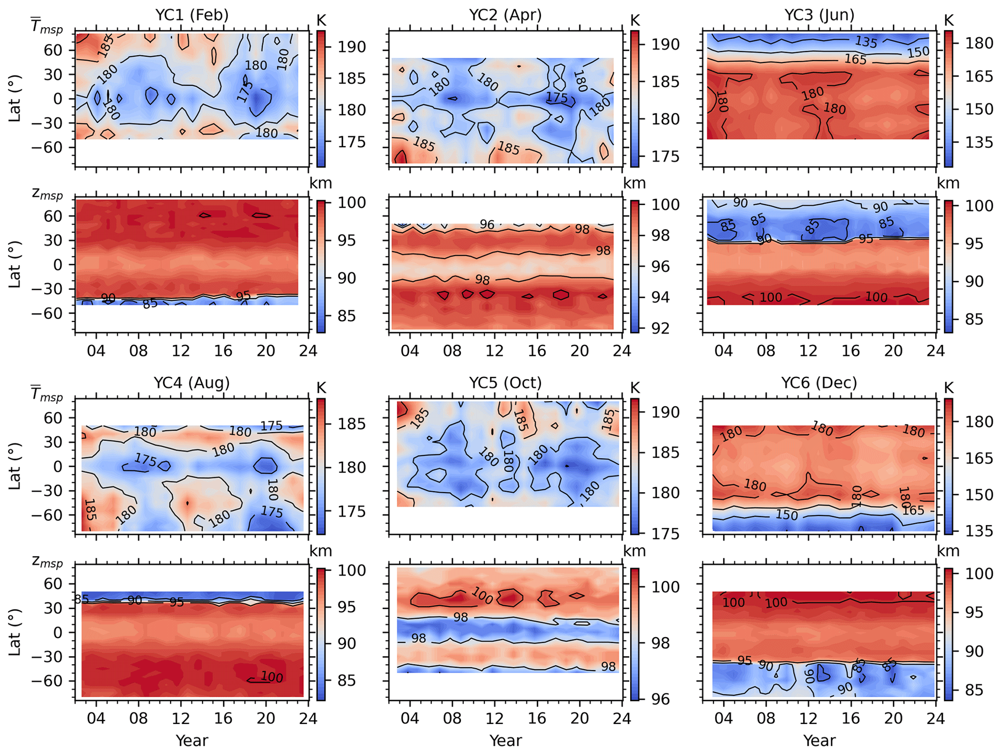
Figure 3 The date–latitude distributions of the mesopause temperature (${\stackrel{\mathrm{‾}}{T}}_{\text{msp}}$, the first and third rows) and altitude (z_msp, the second and fourth rows) calculated from the ${\stackrel{\mathrm{‾}}{T}}_{\text{bcrt}}^{\text{year}}$ of each YC from 2002 to 2023. Here, z_msp is interpolated from the pressure level to geometric height.

2.2 Removing seasonal variations from the mean temperature

Figure 1 shows that the center date of each YC shifts forward about 1 month from 2002 to 2023. This forward drift propagates the seasonal variation in the temperature into ${\stackrel{\mathrm{‾}}{T}}_{\text{bk}}$. This could further distort the long-term trend calculated from ${\stackrel{\mathrm{‾}}{T}}_{\text{bk}}$ and can be removed with the help of MSIS2.0. This is because MSIS2.0 has assimilated the SABER temperature profiles during 2002–2016. The climatological temperature of MSIS2.0 coincides with that of SABER within the uncertainties of ∼ 3 K in the MLT region (Emmert et al., 2021). The detailed procedure for removing seasonal variations is described below.

Firstly, we calculate the mean temperature of MSIS2.0. The temperature profiles (at 15 longitudes and 24 LTs each day) are calculated from MSIS2.0 under conditions of lower solar activity (F_10.7 = 50 SFU, where SFU denotes solar flux units) and geomagnetic quiet time (Ap = 4 nT) throughout 1 calendar year. Therefore, solar and geomagnetic activities do not influence the seasonal variation or trend in the mean temperature. Then, the daily zonal mean is calculated for the temperature profiles of each day. This removes tides and long-period planetary waves. The daily zonal mean temperature in each YC is averaged to get the mean temperature (${\stackrel{\mathrm{‾}}{T}}_{\text{MSIS}}^{\text{year}}$, where the superscript denotes the YC in that year). Figure 2a1 and a2 show the ${\stackrel{\mathrm{‾}}{T}}_{\text{MSIS}}^{\text{year}}$ at 70° N in YC3 and at 70° S in YC6, respectively, during 2002–2023.

Secondly, we calculate the seasonal variations in each YC. The seasonal variations ($\mathrm{\Delta }{\stackrel{\mathrm{‾}}{T}}_{\text{MSIS}}^{\text{year}}$) caused by the forward drift in each YC in different years are quantified by the difference between the ${\stackrel{\mathrm{‾}}{T}}_{\text{MSIS}}^{\text{year}}$ of that year and the reference year (i.e., ${\stackrel{\mathrm{‾}}{T}}_{\text{MSIS}}^{\mathrm{2002}}$). For example, the difference between 2003 and 2002 is calculated as $\mathrm{\Delta }{\stackrel{\mathrm{‾}}{T}}_{\text{MSIS}}^{\mathrm{2003}}={\stackrel{\mathrm{‾}}{T}}_{\text{MSIS}}^{\mathrm{2003}}-{\stackrel{\mathrm{‾}}{T}}_{\text{MSIS}}^{\mathrm{2002}}$. More specifically, as ${\stackrel{\mathrm{‾}}{T}}_{\text{MSIS}}^{\text{year}}$ does not include the year-to-year variations in temperature but depends on the temporal span of the YC only, $\mathrm{\Delta }{\stackrel{\mathrm{‾}}{T}}_{\text{MSIS}}^{\mathrm{2003}}$ in YC3 represents the seasonal variation from 20 to 19 June. Figure 3b1 and b2 show $\mathrm{\Delta }{\stackrel{\mathrm{‾}}{T}}_{\text{MSIS}}^{\text{year}}$ at 70° N in YC3 and at 70° S in YC6, respectively, during 2002–2023. It is evident that the forward drift in the YC induces temperature variations of ± 20 K at 70° N/S from 2002 to 2023 and should be removed before we determine the long-term trends in SABER temperature.

Table 1 The date range of each YC and its corresponding season in the reference year of 2003.

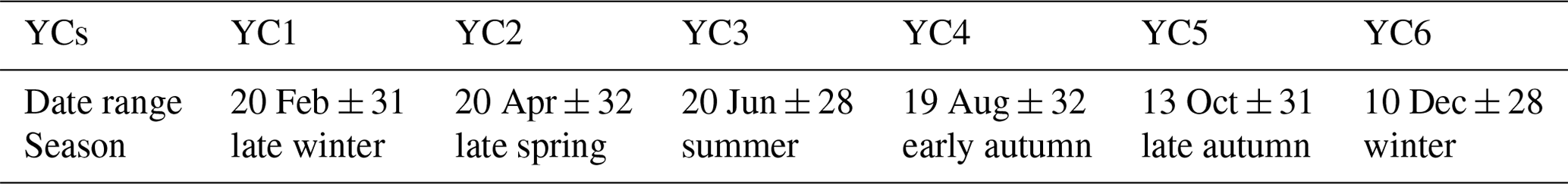
Finally, we correct the mean temperature. The corrected mean temperature (${\stackrel{\mathrm{‾}}{T}}_{\text{bcrt}}^{\text{year}}$, shown in Fig. 3d1 and d2) is obtained by removing $\mathrm{\Delta }{\stackrel{\mathrm{‾}}{T}}_{\text{MSIS}}^{\text{year}}$ from ${\stackrel{\mathrm{‾}}{T}}_{\text{bk}}^{\text{year}}$. This removes the seasonal variation caused by the forward drift in the YC from 2002 to 2023. Moreover, ${\stackrel{\mathrm{‾}}{T}}_{\text{bcrt}}^{\text{year}}$ retains the long-term trend in the mean temperature. We note that, after removing $\mathrm{\Delta }{\stackrel{\mathrm{‾}}{T}}_{\text{MSIS}}^{\text{year}}$, the ${\stackrel{\mathrm{‾}}{T}}_{\text{bcrt}}^{\text{year}}$ covered by each YC can be represented by its center date and half-span in the reference year (Table 1). Table 1 also lists the approximate season related to each YC.

2.3 Determining the long-term trend in the mean temperature

To calculate accurate trends in the MLT region, multiyear variations should be removed properly. The multiyear variations in temperature in the MLT region could be the solar cycle, with a period of about 11 years (Beig et al., 2008; Tapping, 2013; Forbes et al., 2014; Gan et al., 2017; Qian et al., 2019), and the influences from below, such as the El Niño–Southern Oscillation (ENSO) with varying cycles of around 2–7 years (Domeisen et al., 2019; Li et al., 2013, 2016; Randel et al., 2009). The solar cycle can be represented by the solar radiation flux at 10.7 cm (i.e., F_10.7, with units of SFU = 10⁻²² $\mathrm{W}{\mathrm{m}}^{-\mathrm{2}}{\mathrm{Hz}}^{-\mathrm{1}}$) (Tapping, 2013). ENSO is represented by the multivariate ENSO index (MEI) (Domeisen et al., 2019). The multiple linear regression (MLR) method is effective to separate the long-term trend in temperature from the variations caused by the solar cycle, ENSO, and the quasi-biennial oscillation (QBO). The MLR equation is formulated as follows:

$$\begin{array}{}\text{(3)}& Y\left(t\right)=c_{\mathrm{0}}+c_{\mathrm{1}}t+c_{\mathrm{2}}{F}_{\mathrm{10.7}}\left(t\right)+c_{\mathrm{3}}\text{ENSO}\left(t\right)+\mathit{\epsilon }\left(t\right).\end{array}$$

Here, Y represents the mean temperature at year t from 2002 to 2023; c₀ represents a mean state of Y; c₁ is the long-term trend in Y; and c₂ and c₃ represent the contributions from the solar cycle and ENSO, respectively. The terms for F_10.7 and ENSO are included in Eq. (3) for the purpose of correctly determining the long-term trend, but they are not considered further in this work. Here, we note that both the trends (linear variations) and quasi-periodic variations represent the natural variations in the predictors. These natural variations might influence the trends and variations in temperature. Thus, MLR is applied to characterize the contributions from the natural variations in predictors. The resulting trends in the temperature then exclude the trends inhibited in the predictors. This is the trend studied in this work. Otherwise, if these predictors are detrended, their residuals are used in the MLR. Thus, the resulting trends in temperature may include the trends inhibited in the predictors.

The statistical significance of the regression coefficients is measured using a Student t test and the variance–covariance matrix in Eq. (3). Specifically, in Eq. (3), the sampling points are 22 and the predictor variables are 4. This results in 19 degrees of freedom. Consequently, the critical value is ∼ 2.0 based on a Student t test at a confidence level of 95 % (Kutner et al., 2005). This signifies that, with reference to a 95 % confidence level, the magnitude of the regression coefficient should be at least 2.1 times greater than the standard deviation.

2.4 Determining the mesopause of each yaw cycle

The mesopause temperature (${\stackrel{\mathrm{‾}}{T}}_{\text{msp}}$) is defined as the minimum of the mean temperature. The pressure level at which the minimum temperature occurs is defined as the mesopause altitude (z_msp). Figure 2d1 and d2 show the mesopause altitudes calculated from ${\stackrel{\mathrm{‾}}{T}}_{\text{bk}}^{\text{year}}$ (black crosses) and ${\stackrel{\mathrm{‾}}{T}}_{\text{bcrt}}^{\text{year}}$ (red dots), respectively. We see that the mesopause altitudes calculated from ${\stackrel{\mathrm{‾}}{T}}_{\text{bk}}^{\text{year}}$ and ${\stackrel{\mathrm{‾}}{T}}_{\text{bcrt}}^{\text{year}}$are nearly identical in the first several years but exhibit discrepancies over the later several years. This implies that the seasonal variation caused by the forward drift in the YC affects the mesopause altitudes to some extent. Moreover, the mesopause altitudes exhibit larger variabilities in the southern summer polar region (YC6) compared with the northern summer polar region (YC3). Figure 3 shows the date–latitude distributions of the mesopause temperature (${\stackrel{\mathrm{‾}}{T}}_{\text{msp}}$) and altitude (z_msp) calculated from ${\stackrel{\mathrm{‾}}{T}}_{\text{bcrt}}^{\text{year}}$. We note that z_msp is initially defined for the pressure level (Fig. 2d). To compare our work with previous studies, z_msp is interpolated onto the geometric heights in Fig. 3.

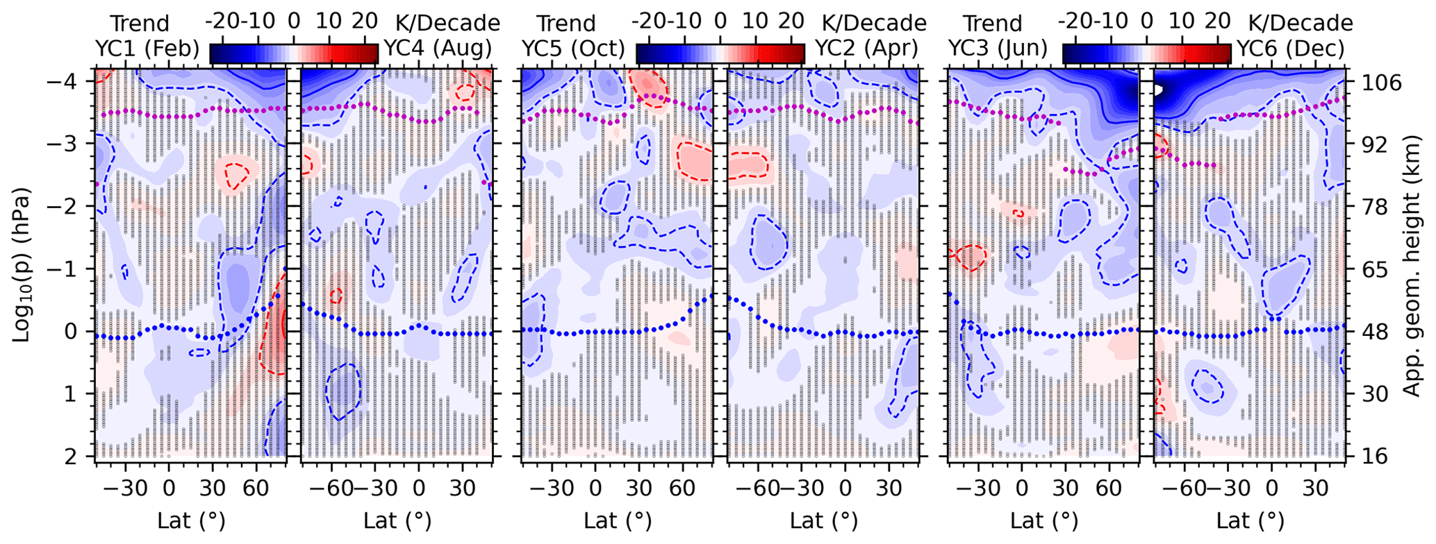
Figure 4 Trends in the corrected mean temperature in the six YCs. The solid and dashed contour lines indicate ± 6 and ± 2 K per decade, respectively. The purple and blue dots indicate the heights of the mesopause and stratopause, respectively. The regions marked by shaded points indicate that trends are not significant with reference to a 95 % confidence level. The approximate geometric height is label on the last subpanel.

Previous SABER studies have often discarded high latitudes, possibly due to insufficient LT coverage that induces uncertainties in the mean temperature estimation. A major advantage of binning the SABER temperature based on YC is that an accurate mean temperature can be obtained. Thus, the latitudinal variations in ${\stackrel{\mathrm{‾}}{T}}_{\text{msp}}$ and z_msp at high latitudes can be thoroughly studied. Firstly, we focus on the YCs in northern summer and winter (i.e., YC3 and YC6, respectively), as the summer mesopause at high latitudes is more sensitive to the summer-to-winter circulation (Dunkerton, 1978; Qian et al., 2017). In YC3 (YC6), ${\stackrel{\mathrm{‾}}{T}}_{\text{msp}}$ and z_msp generally decrease from 50° S to 80° N (50° N to 80° S). We note that ${\stackrel{\mathrm{‾}}{T}}_{\text{msp}}$ has local minima around the Equator throughout the 22 years in YC3 and YC6 and is the coldest at the highest latitudes of the summer hemisphere. The z_msp is the lowest at 40–60° N/S throughout the 22 years. Besides the latitudinal variations, ${\stackrel{\mathrm{‾}}{T}}_{\text{msp}}$ and z_msp also exhibit multiyear variations. For example, ${\stackrel{\mathrm{‾}}{T}}_{\text{msp}}$ is colder around the Equator during the solar minima (i.e., 2007–2008 and 2019–2021) in YC3 and YC6. In YC6, the lower z_msp at southern higher latitudes might be related to the warm phase of ENSO during 2002–2005 and 2016–2019.

In YC2 and YC5, the latitudinal variations in ${\stackrel{\mathrm{‾}}{T}}_{\text{msp}}$ and z_msp are almost hemispherically symmetrical. The ${\stackrel{\mathrm{‾}}{T}}_{\text{msp}}$ is the coldest around the Equator and the warmest at the highest latitudes. The z_msp is the lowest at lower latitudes and the highest at the highest latitudes. In YC1, ${\stackrel{\mathrm{‾}}{T}}_{\text{msp}}$ and z_msp share similar latitudinal variations in winter (YC6); the difference is that ${\stackrel{\mathrm{‾}}{T}}_{\text{msp}}$ is warmer in YC1 than in YC6, while z_msp is higher in YC1 than in YC6. In YC4, ${\stackrel{\mathrm{‾}}{T}}_{\text{msp}}$ and z_msp share similar latitudinal variations in summer (YC3); the difference is that ${\stackrel{\mathrm{‾}}{T}}_{\text{msp}}$ is warmer in YC4 than in YC3, while z_msp is higher in YC4 than in YC3. In YC1–YC2 and YC4–YC5, multiyear variations in ${\stackrel{\mathrm{‾}}{T}}_{\text{msp}}$ exhibit clear a dependence on the solar cycle. At lower latitudes, ${\stackrel{\mathrm{‾}}{T}}_{\text{msp}}$ values are colder during the solar minima (i.e., 2006–2010 and 2017–2021). At high latitudes, ${\stackrel{\mathrm{‾}}{T}}_{\text{msp}}$ values are warmer during the solar maxima (i.e., 2002–2005, 2012–2014, and after 2021). However, it seems that the multiyear variations in z_msp are not as obvious as those in ${\stackrel{\mathrm{‾}}{T}}_{\text{msp}}$. These multiyear variations are considered in Eq. (3) to separate the long-term trend in ${\stackrel{\mathrm{‾}}{T}}_{\text{msp}}$ correctly, but they are not considered further in this work.

3 Trends in temperature in the MLT region and mesopause

3.1 Trends in temperature in the MLT region

Trends in the corrected mean temperature and their significance for each YC are shown in Fig. 4. These trends are generally larger at high latitudes than those at lower latitudes within the six YCs. Moreover, the trends show both hemispheric symmetry and asymmetry approximately in the high-latitude MLT region.

First, we describe the hemispheric symmetry in the trends. In YC1 and YC4 and above 10⁻³ hPa, the cooling trends are ≥ 2 K per decade at latitudes higher than 40° N (YC1) and 40° S (YC4), respectively. Around 10⁻⁴ hPa, the cooling trends reach their peaks of ≥ 6 K per decade. In addition, there are also warming trends of ≥ 2 K per decade at latitudes higher than 30° S (YC1) and 30° N (YC4), respectively. Above the mesopause, there are cooling trends of ≥ 2 K per decade observed within the latitude range of 20–50° S for YC5 and 20–50° S for YC2. Additionally, in the region just below 10⁻³ hPa, there are warming trends of ≥ 2 K per decade at latitudes of 50–80° N for YC5 and 50–80° S for YC2. In YC3 and YC6, the cooling trends of ≥ 2 K per decade shift upward from the mesopause at 80° N (YC3) and 80° S (YC6) to 10⁻⁴ hPa at 50° S (YC3) and 50° N (YC6). There are also cooling trends of ≥ 6 K per decade at the high latitudes of the summer hemisphere. Meanwhile, the coldest trends are ≥ 10 K per decade just below 10⁻⁴ hPa and at 80° N/S. Although the cooling trends in the MLT region have been reported extensively at lower and middle latitudes (Beig et al., 2003; Laštovička, 2023), the extreme cooling trends at high latitudes and above the summer mesopause have not yet been reported. We note that the systematic error in the SABER operational processing is unknown. Its impacts on the credibility of the trends derived here will be discussed in Sect. 4.

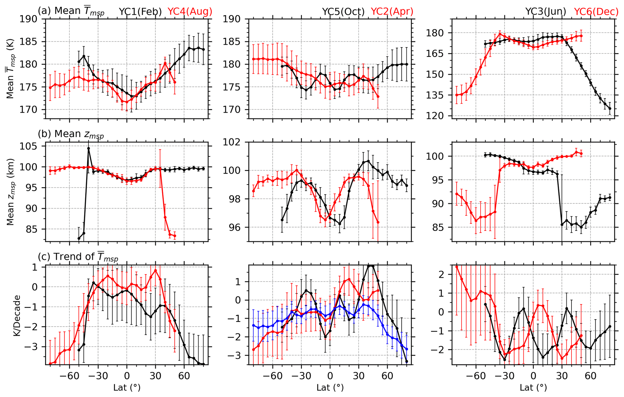
Figure 5 Latitudinal variations in the means of the mesopause temperature (${\stackrel{\mathrm{‾}}{T}}_{\text{msp}}$, a) and altitude (z_msp, b) and the trends in the ${\stackrel{\mathrm{‾}}{T}}_{\text{msp}}$ (c) of the six YCs during 2002–2023. The error bars for each YC indicate 2.1 times the standard deviation (i.e., at a 95 % confidence level according to a Student t test). The all-YC mean trend in the mesopause temperature is shown as a blue line in the middle subpanel of panel (c).

Next, we describe the hemispheric asymmetry in the trends. In YC1 and YC4, the cooling trends of ≥ 2 K per decade in YC1 extend to a wider latitude range (20° N–80° S) than those in YC4 (30° S–80° S) above 10⁻³ hPa. The insignificant warming trends of ≥ 2 K per decade can be seen in the stratosphere at latitudes higher than 60° N in YC1 but at 45–60° S in YC4. In YC5 and YC2, the cooling trends of ≥ 2 K per decade can be seen around the stratopause at 30–50° S (YC5) but below the stratopause at 30–50° N (YC2). In YC3 and YC6, the significant warming trends of ≥ 2 K per decade in YC6 are stronger than those in YC3 around 0.1 hPa. In addition, the warming trends near the summer mesopause are significant in YC6 but insignificant in YC3. The simulation results in Qian et al. (2019) also demonstrated warming trends in the southern summer MLT region. Specifically, they showed significant warming trends below ∼ 95 km and cooling trends above ∼ 95 km at latitudes exceeding 45° S between November and February. In contrast, there were insignificant or warming trends at latitudes exceeding 45° N during June and July. Qian et al. (2019) attributed the warming trend in the summer mesosphere to the changing meridional circulation.

3.2 Structure and trends in the mesopause

Taking advantage of the continuous long-term (22 years or equivalently two solar cycles) measurements and binning the YCs at 50° S–80° N or 80° S–50° N, the robust mean states of the mesopause temperature (${\stackrel{\mathrm{‾}}{T}}_{\text{msp}}$) and height (z_msp) as well as their trends and the responses of ${\stackrel{\mathrm{‾}}{T}}_{\text{msp}}$ to the solar cycle, ENSO, and QBO are quantified using MLR. Here, we focus on the mean states and trends in the mesopause temperature and altitude.

Figure 5a and b show the mean ${\stackrel{\mathrm{‾}}{T}}_{\text{msp}}$ and z_msp over 22 years for the six YCs. In YC1–YC2 and YC4–YC5, the mean ${\stackrel{\mathrm{‾}}{T}}_{\text{msp}}$ is in the range of 172–183 K. However, the mean ${\stackrel{\mathrm{‾}}{T}}_{\text{msp}}$ at latitudes higher than 40° N is warmer in YC1 compared with YC5, and the mean ${\stackrel{\mathrm{‾}}{T}}_{\text{msp}}$ at latitudes higher than 40° S is warmer in YC2 compared with YC4. The mean z_msp is mainly in the range of ∼ 96–102 km, but it is higher than ∼ 85 km at 40–50° N (YC1) and 40–50° N (YC4). In YC3, the mean ${\stackrel{\mathrm{‾}}{T}}_{\text{msp}}$ decreases sharply with latitude, from ∼ 180 K at 30° N to ∼ 125 K at 80° N. The mean z_msp in YC3 reaches a minimum of ∼ 85 km at 60° N. In YC6, the mean ${\stackrel{\mathrm{‾}}{T}}_{\text{msp}}$ decreases sharply with latitude, from ∼ 180 K at 35° S to ∼ 135 K at 80° S. The mean z_msp in YC6 reaches a minimum of ∼ 86 km at ∼ 50° S. The mean ${\stackrel{\mathrm{‾}}{T}}_{\text{msp}}$ (z_msp) in the northern summer polar region is ∼ 5–11 K (∼ 1 km) colder (lower) than that in the corresponding southern region. The hemispheric asymmetries of the summer mesopause temperature and altitude coincide with Xu et al. (2007), who used the SABER temperature data during 2002–2006 and showed that the mean ${\stackrel{\mathrm{‾}}{T}}_{\text{msp}}$ in the summer polar region of the NH is ∼ 5–10 K colder than its counterpart in the SH. A recent study by Wang et al. (2022), who used the SABER temperature data during 2002–2020, showed that the mean ${\stackrel{\mathrm{‾}}{T}}_{\text{msp}}$ in the summer polar region of the NH is ∼ 10 K colder than its counterpart in the SH. Moreover, the transition latitudes of the mean ${\stackrel{\mathrm{‾}}{T}}_{\text{msp}}$ (z_msp) from higher temperature (height) are 30° N in YC3 and 40° S in YC6. This coincides well with values reported by Xu et al. (2007) and Wang et al. (2022). These hemispheric asymmetries of the mean ${\stackrel{\mathrm{‾}}{T}}_{\text{msp}}$ and z_msp as well as the transition latitudes could be caused by the hemispheric asymmetry of solar radiation and gravity wave forcing (Xu et al., 2007).

Figure 5c shows that trends in ${\stackrel{\mathrm{‾}}{T}}_{\text{msp}}$ in YC1 and YC4 display extreme cooling (≥ 2 K per decade) at latitudes higher than 55° N/S. However, at 40° S–40° N, trends in ${\stackrel{\mathrm{‾}}{T}}_{\text{msp}}$ in YC1 show cooling, with magnitudes of ∼ 0–2 K per decade, whereas they show warming in YC4, with magnitudes of ∼ 0–1 K per decade. In YC2 and YC5, trends in ${\stackrel{\mathrm{‾}}{T}}_{\text{msp}}$ show either cooling or warming, depending on the specific latitudes and months being considered. At southern latitudes, trends in ${\stackrel{\mathrm{‾}}{T}}_{\text{msp}}$ show cooling, with magnitudes of ≥ 1 K per decade in YC2. Trends in ${\stackrel{\mathrm{‾}}{T}}_{\text{msp}}$ in YC5 change sharply from 2.0 K per decade at 45° N to −3 K per decade at 80° N. In YC3 and YC6, trends in ${\stackrel{\mathrm{‾}}{T}}_{\text{msp}}$ mainly show cooling, except for the insignificant warming trends in YC6 and at latitudes higher than 40° S. Although trends in ${\stackrel{\mathrm{‾}}{T}}_{\text{msp}}$ show warming at some latitudes in certain YCs, the all-YC mean trends in ${\stackrel{\mathrm{‾}}{T}}_{\text{msp}}$ (blue line in Fig. 5c) show cooling, with magnitudes of 0.3–1 K per decade at 50° S–50° N. At latitudes higher than 55° S, the insignificant cooling trends are ≤1.5 K per decade. In contrast, at latitudes higher than 55° N, the significant cooling trends are ≥ 1.5 K per decade.

4 Discussion

The trends derived here may be influenced by the unknown systematic errors in the SABER operational processing. The main causes of systematic errors are the lack of accurate knowledge of the uncertainties in key parameters (mixing ratios of atomic oxygen, O, and carbon dioxide, CO₂) and the nature of non-LTE (local thermodynamic equilibrium) in the SABER temperature retrieval. The O mixing ratio provided to the SABER operational processing is from NRLMSISE-00 (Picone et al., 2002). Below 100 km, no atmospheric observations of O are incorporated. Thus, the uncertainty in O influences the uncertainties in temperature at ∼ 75–110 km, in particular at 100–110 km. The CO₂ mixing ratio provided to the SABER operational processing is the monthly average value from the WACCM model (Dawkins et al., 2018; Mlynczak et al., 2023). Thus, there is no LT variation in the CO₂ used in the SABER operational processing. The larger vertical diffusion used in WACCM4 compared with WACCM3 led to a 15 % uncertainty in CO₂ at 110 km. Mlynczak et al. (2023) showed that a 15 % uncertainty in CO₂ at 110 km results in an 8 K error in the global-mean (55° S–55° N) temperature. Moveover, the lack of correct trends and their coupling with dynamic adjustments in O and CO₂ may also be sources of systematic errors in the SABER temperature at high altitudes. At high altitudes and latitudes, non-LTE radiative transfer in CO₂ couples the vibrational temperatures at all altitudes due to the exchange of radiation among all layers. Thus, any uncertainties in O or CO₂ at one layer will affect the temperature at all altitudes. These uncertainties are systematic errors and cannot be reduced by averaging many profiles. Therefore, the trends derived here should be discussed rigorously based on the systematic errors in a single temperature profile.

As reported on the SABER website (https://spdf.gsfc.nasa.gov/pub/data/timed/saber/, last access: 31 January 2024), 1 standard deviation (corresponding to a confidence level of 68 %) in the systematic error for a single temperature profile is ∼ 1.4 K at and below 80 km, 4.0 K at 90 km, 5.0 K at 100 km, and 25.0 K at 110 km for typical midlatitude conditions. These errors may be larger at high latitudes. A rigorous systematic error analysis is performed by assuming a negative systematic error (−E) in 2002 and a positive systematic error (+E) in 2023. The difference between the two numbers over the 22 years is the largest uncertainty caused by the systematic error (i.e., 2$E/\mathrm{22}\approx \mathrm{0.09}E$ K yr⁻¹, or 0.9E K per decade) and is referred to as the systematic trend uncertainty. The number E is then replaced by the systematic error reported on the SABER website. Thus, one can obtain a systematic trend uncertainty for a given systematic error. We note that the systematic trend uncertainty of 0.9E K per decade is the largest uncertainty caused by the systematic error and is the worst-case scenario among all of the combinations of systematic errors in different years.

Based on the systematic error defined by 1 standard deviation on the SABER website, the systematic trend uncertainty during 2002–2023 caused by systematic errors at 110 km (∼ log₁₀ (6.3 × 10⁻⁵ hPa) = −4.2) can be estimated as 50 K/22 years ≈ ± 2.27E K yr⁻¹, or 22.7E K per decade. In the same manner, the systematic trend uncertainties are 4.5 K per decade at 100 km (∼ log₁₀ (2.8 × 10⁻⁴ hPa) = −3.6), 3.6 K per decade at 90 km (∼ log₁₀ (1.4 × 10⁻³ hPa) = −2.9), and 1.3 K per decade at and below 80 km (∼ log₁₀ (6.6 × 10⁻³ hPa) = −2.2). We note that the systematic trend uncertainty will be doubled if the systematic error is defined by 2 times the standard deviation (corresponding to a confidence level of 95 %). In the following discussions, we will compare the trends derived here with previous observations and the systematic trend uncertainty calculated from the systematic error defined by 1 standard deviation. If the derived trend is larger than the systematic trend uncertainty, the trend is reliable; otherwise, the trend is questionable.

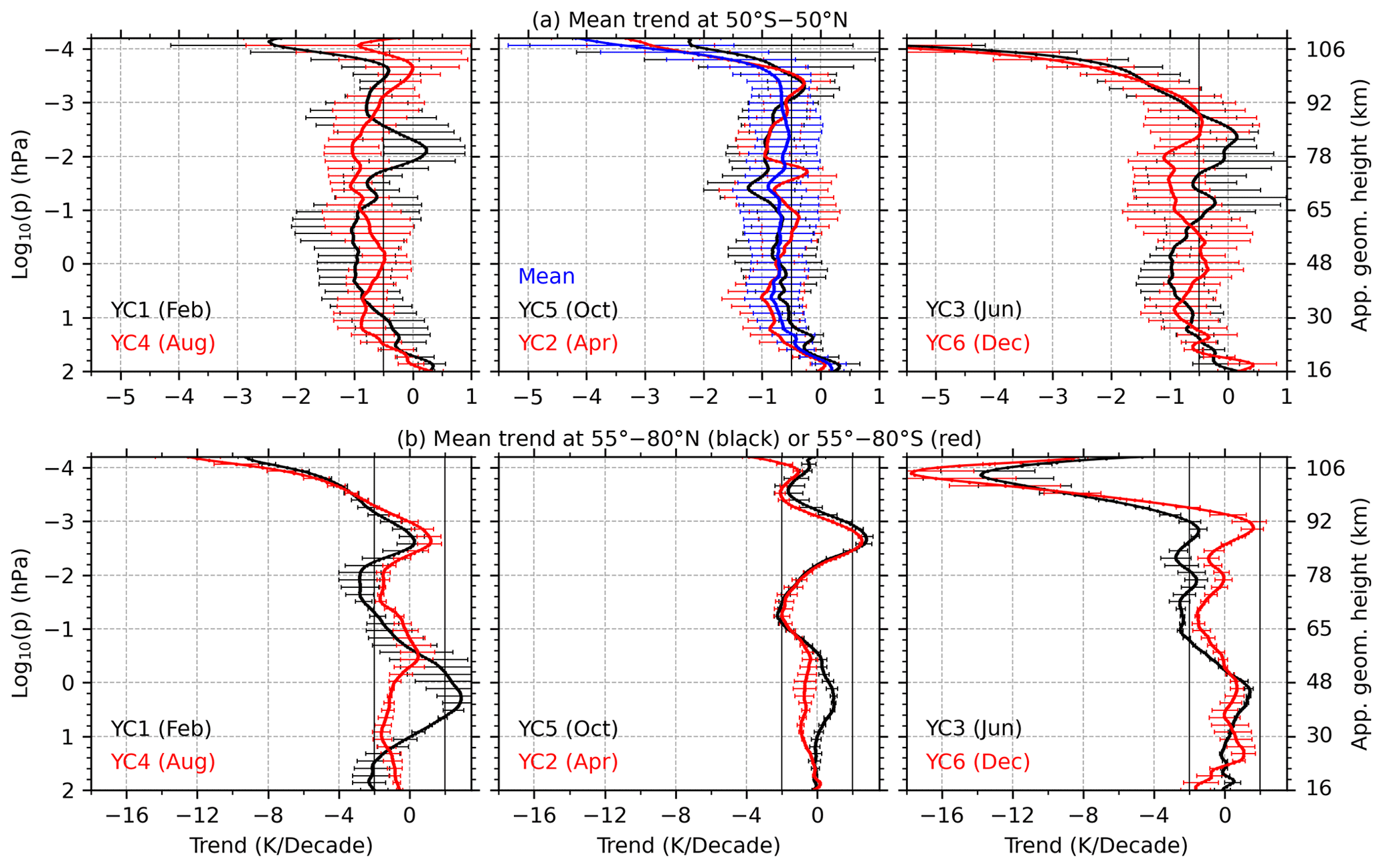
Figure 6 Mean trends in the corrected mean temperature at 50° S–50° N (a) and at 55–80° S (red line in panel b) or 55–80° N (black line in panel b) for the six YCs. The annual mean trend is calculated by averaging the trends in the six YCs at 50° S–50° N and is shown as a blue line in the middle subpanel of panel (a). The error bars indicate the standard errors in the averaged data.

The temporal interval of the data may also influence the long-term trend (Laštovička and Jelínek, 2019). Using the nocturnal temperature in the MLT region measured by lidar instruments around 41° N and 42° N over the period from 1990 to 2017, She et al. (2019) demonstrated that the cooling trends are ∼ 2.0–4.5 K per decade over only one solar cycle, whereas they are ∼ 2.0–2.5 K per decade if the data series is longer than two solar cycles. Using the SABER temperature profiles during 2002–2019, Zhao et al. (2020) showed that the significant trends in ${\stackrel{\mathrm{‾}}{T}}_{\text{msp}}$ and their responses to the solar cycle can be obtained at 50° S–50° N over longer than one solar cycle. Both She et al. (2019) and Zhao et al. (2020) showed that the trends are relatively insensitive to the specific beginning and ending time of the data compared with the data series length. As the data series length used in this study spans approximately two solar cycles, the derived trends are reliable in a statistical sense. In the following discussion, the reliability of trends will also be determined by comparing them with the systematic trend uncertainty.

4.1 The reliability of trends in the MLT region at latitudes lower than 50° N/S

To facilitate a comparison with previously reported annual and global-mean trends in the MLT region, we present the mean trends in the corrected mean temperature at 50° S–50° N and at 55–80° S or 55–80° N for the six YCs (Fig. 6). The mean trends at 50° S–50° N for each YC show cooling, with magnitudes of ∼ 0.5–1 K per decade at 10–10⁻³ hPa. The exception is the warming trend of 0.2 K per decade around 10⁻² hPa in YC1 and of 0.1 K per decade around 4 × 10⁻³ hPa in YC3. Above 5 × 10⁻³ hPa, the cooling trends increase sharply with altitude and reach ∼ 2 K per decade in YC5 and ∼ 3 K per decade in YC2 at 10⁻⁴ hPa. Compared with the situation in YC2 and YC5, the cooling trends increase more sharply with altitude in YC3 and YC6. Their magnitudes change nearly identically and are from ∼ 0.5 K per decade at 2 × 10⁻³ hPa to ≥ 5 K per decade at 10⁻⁴ hPa. When the mean trends at 50° S–50° N across all YCs are further averaged, we obtain an annual mean trend (blue line in Fig. 6a). The annual mean trend shows cooling, with magnitudes of ∼ 0.5–0.8 K per decade that vary slightly with altitude at 10 × 10⁰–5 × 10⁻⁴ hPa.

The altitude variation and the magnitude of the annual mean trend are similar to previous results (Garcia et al., 2019; Mlynczak et al., 2022; Zhao et al., 2021). Figure 3 of Garcia et al. (2019) revealed that the global-mean (52° S–52° N) SABER temperature trends display cooling, with magnitudes of ∼ 0.5–0.9 K per decade at 10–5 × 10⁻⁴ hPa during 2002–2018. These magnitudes of these cooling trends are slightly smaller than those derived from WACCM. Table 1 of Mlynczak et al. (2022) demonstrated that the global-mean (55° S–55° N) SABER temperature also displays cooling trends, with magnitudes of ∼ 0.51–0.63 K per decade at 1–10⁻³ hPa. Similarly, Fig. 4 of Zhao et al. (2021) revealed that the global-mean (50° S–50° N) SABER temperature trends show cooling, with magnitudes of ∼ 0.5–0.9 K per decade at 30–105 km. At 10⁻⁴ hPa, the extreme cooling trend of 2.6 K per decade in Table 1 of Mlynczak et al. (2022) is slightly smaller than the 2.8 K per decade derived here, although within 2 times the standard deviation (blue line in Fig. 6a). By further examining the trends across the six YCs (Figs. 4 and 6a), it becomes evident that the extreme cooling trend is mainly attributed to the middle latitudes of the summer hemisphere (i.e., YC3 and YC6), although also partially to other months. As suggested by Mlynczak et al. (2022), the extreme cooling trend at 10⁻⁴ hPa is due to a decrease in solar irradiance that is not captured by the F_10.7 index.

We note that these trends are derived from the SABER temperature. The systematic error in the SABER temperature influences the credibility of these derived trends. According to the rigorous analysis of the systematic error, the trends derived here are reliable only if their magnitudes are larger than the systematic trend uncertainty. The annual and global-mean trends that show cooling with magnitudes of 2–4 K per decade around 10⁻⁴ hPa are unreliable, as these values are in the range of the systematic trend uncertainty of 22.7 K per decade at 6.3 × 10⁻⁵ hPa and 4.5 K per decade at 2.8 × 10⁻⁴ hPa. At pressure levels lower than 10⁻³ hPa, the annual and global-mean trends that show cooling with magnitudes of ∼ 0.5–1 K per decade are unreliable, as these values are in the range of the systematic trend uncertainty of 3.6 K per decade around 10⁻³ hPa and 1.3 K per decade below 6.6 × 10⁻³ hPa.

These detailed comparisons showed that the trends at the pressure levels reported by Garcia et al. (2019) and Mlynczak et al. (2022) directly support the altitude variations and magnitudes of the trends derived here. Although the trends reported by Zhao et al. (2021) are for the geometric height, their altitude variations and magnitudes also agree with the trends derived here. However, these trends are unreliable, as their magnitudes are in the range of the systematic trend uncertainties. We note that the method of binning SABER observations based on the YC provides an opportunity to study the trends at latitudes higher than 50° N/S in certain months.

4.2 The reliability of trends in the MLT region at latitudes higher than 50° N/S

At latitudes higher than 50° N/S, the altitude variations in the mean trends in the six YCs (Fig. 6b) are seasonally symmetrical above approximately 1 hPa. The magnitudes of trends are mainly in the range of −2 to 2 K per decade below a height of 10⁻³ hPa. These trends are larger than the systematic trend uncertainties of 1.3 K per decade and, thus, are reliable below 6.6 × 10⁻³ hPa. Moreover, these trends are in the range of the systematic trend uncertainties of 3.6 K per decade and, thus, are unreliable around 10⁻³ hPa. An interesting feature is the warming trends of 1–2.5 K per decade at 10⁻²–10⁻³ hPa in April, August, October, and December. The altitudes of peaks in the warming trends vary from 4 × 10⁻³ hPa to 10⁻³ hPa in different months. Focusing on the latitude band of 64–70° N in June and 64–70° S in December, Bailey et al. (2021) merged the temperature data from HALO and SABER (total length of 29 years) and from HALOE and SOFIE (total length of 22 years). Their analysis revealed warming trends of 1–2 K per decade near 5 × 10⁻³ hPa (∼ 85 km) at 64–70° N in June and 64–70° S in December, as illustrated in Fig. 7 of their paper. The results simulated by WACCM-X showed significant warming trends at ∼ 80–95 km at latitudes higher than 45° S from November to February and close to zero or warming trends at latitudes higher than 45° N from June to July (Qian et al., 2019). The warming trends in December derived here coincide with those reported by Bailey et al. (2021) and Qian et al. (2019). The weak warming trend at 2 × 10⁻³ hPa in June coincides with those in Qian et al. (2019) but is much smaller than the 1–2 K per decade reported by Bailey et al. (2021). In April and October, the warming trends are hemispherically symmetrical at 10⁻²–10⁻³ hPa and reach a peak of ≥ 2 K per decade at 3 × 10⁻³ hPa. It should be noted that the warming trends of 1–2.5 K per decade at 10⁻²–10⁻³ hPa are in the range of the systematic trend uncertainties of 1.3 K per decade at 6.6 × 10⁻³ hPa and 3.6 K per decade around 10⁻³ hPa; thus, they are unreliable in the sense of systematic trend uncertainty. Above 10⁻³ hPa, the trends transit from warming to cooling.

We can see extreme cooling trends of ≥ 6 K per decade above ∼ 10⁻³ hPa in YC3 and YC6 as well as around 10⁻⁴ hPa in YC1 and YC4. Due to the systematic trend uncertainty, these trends are reliable around 10⁻³ hPa but unreliable around 10⁻⁴ hPa. These cooling trends are comparable with the global average mesosphere temperature of 6.8–8.4 K per decade derived by Mlynczak et al. (2022) after doubling the CO₂ in the MLT region. However, it takes decades to double CO₂. Thus, a purely radiative effect due to increasing CO₂ cannot support the extreme cooling trends derived here. Mlynczak et al. (2022) proposed that the F_10.7 is not a suitable proxy to indicate the effects of solar radiation on the lower thermosphere. However, the solar irradiance in the Schumann–Runge band (175–200 nm) might be responsible for the colder trend. Even so, the extreme cooling trends of ∼ 10 K per decade are still larger than those reported by Mlynczak et al. (2022). Other possible reasons for these extreme cooling trends in the high-latitude MLT region can be attributed to the dynamic feedback in the polar MLT region.

Besides the purely radiative effect on the cooling trends in the MLT region (i.e., Garcia et al., 2019; Mlynczak et al., 2022), the dynamic feedback might be another cause of the cooling trends. Based on the simplified transformed Eulerian mean (TEM) thermodynamic equation, the temperature change (ΔT) caused by dynamics can be written as follows (Eqs. 3 and 4 of Yu et al., 2023):

$$\begin{array}{}\text{(4)}& \mathrm{\Delta }T=-{\mathit{\alpha }}^{-\mathrm{1}}\left(w^{\ast }S+v^{\ast }{\displaystyle \frac{\partial \stackrel{\mathrm{‾}}{T}}{a\partial \mathit{\phi }}}\right).\end{array}$$

Here, α is the Newtonian cooling coefficient; w^∗ and v^∗ are the residual vertical and meridional velocity, respectively; S and $\stackrel{\mathrm{‾}}{T}$ are the static stability and zonal mean temperature, respectively; and a and φ are the Earth's radius and latitude, respectively. From Eq. (4), we propose that the extreme cooling trends in the high latitudes of the summer hemispheres (YC3 and YC6) might result from the changing summer-to-winter circulation and gravity wave forcing in the MLT region. The circulation is upwelling (positive w^∗) in the summer hemisphere and causes a cold summer mesosphere through adiabatic cooling. Conversely, in the winter hemisphere, the circulation is downwelling (negative w^∗), leading to a warm winter mesosphere through adiabatic warming (Garcia and Solomon, 1985). A necessary condition for the extreme cooling trends at summer high latitudes is the stronger upwelling and, thus, the increasing gravity wave body force in the summer hemispheres. Previous studies have shown that the gravity wave potential energy (GWPE) in the MLT region exhibits significant positive trends at southern high latitudes in January and at northern high latitudes in July (Fig. 5 of Liu et al., 2017). The positive trends in the GWPE might enhance the strength of upwelling and, thus, result in extreme cooling trends in the high latitudes of the summer hemispheres. It should be noted that the dynamic feedback in the MLT region is only analyzed qualitatively, as quantitative analysis should be performed through model simulations. Thus, one can elucidate the physics behind the strong cooling trend in the polar MLT region.

4.3 The reliability of the mesopause trends

The trends in ${\stackrel{\mathrm{‾}}{T}}_{\text{msp}}$ derived in this study are significant and mainly negative at 50° S–50° N across most YCs. The averaged trend in ${\stackrel{\mathrm{‾}}{T}}_{\text{msp}}$ for the six YCs is −0.64 ± 0.22 K per decade over 50° S–50° N. When the average is calculated over 80° S–80° N, the trend in ${\stackrel{\mathrm{‾}}{T}}_{\text{msp}}$ for the six YCs is −1.03 ± 0.40 K per decade. The cooling trend in ${\stackrel{\mathrm{‾}}{T}}_{\text{msp}}$ derived here also coincides with the −0.5 ± 0.21 K per decade trend in the mesosphere (Garcia et al., 2019), although only within 50° S–50° N. Compared with the trend derived from sodium lidar observations during nighttime only around 40° N, the trends in ${\stackrel{\mathrm{‾}}{T}}_{\text{msp}}$ from SABER are about −0.1, 0.0, −0.2, −0.8, 0.6, and −1.9 K per decade for the six YCs and have an annual mean of −0.4 K per decade. This is less than the significant cooling trend of 2.3–2.5 K per decade during 1990–2018 but is consistent with the insignificant cooling trend of 0.2–1 K per decade during 2000–2018 (Yuan et al., 2019). The comparisons of the trends in ${\stackrel{\mathrm{‾}}{T}}_{\text{msp}}$ between our results and those from satellites and ground-based observations exhibit general consistencies in the sense of the annual mean or global mean. However, the z_msp is mainly above 95 km (6.5 × 10⁻⁴ hPa), where the systematic trend uncertainties are larger than 3.8 K per decade and are larger than the trends in ${\stackrel{\mathrm{‾}}{T}}_{\text{msp}}$. Thus, the trends in ${\stackrel{\mathrm{‾}}{T}}_{\text{msp}}$ derived here are mainly unreliable in the sense of rigorous systematic error analysis.

A notable feature is the warming trends in ${\stackrel{\mathrm{‾}}{T}}_{\text{msp}}$ with magnitudes of 0–2 K per decade at latitudes higher than 40° S in YC6. This warming trend is insignificant at a 95 % confidence level. If we change the temporal interval from 2002–2023 to 2002–2019, the trends in ${\stackrel{\mathrm{‾}}{T}}_{\text{msp}}$ are cooling with magnitudes of 1–2 K per decade. Here, we note that the year 2020 is just after the SABER temperature data were revised (version 2.08, from 15 December 2019) (Mlynczak et al., 2023). In this work, we use the SABER temperature data of versions 2.07 (before 15 December 2019) and 2.08 (after 15 December 2019). According to Mlynczak et al. (2023), the newly released data are free from algorithm instability. A recent study by Yu et al. (2023) showed that the Hunga Tonga–Hunga Ha'apai (HTHH) volcanic eruption on 15 January 2022 induced temperature anomalies of ± 10 K globally in the stratosphere and mesosphere in August. The anomalies disappeared after September 2022. This indicates that this volcanic eruption may have influenced the mesosphere temperature through circulations and waves. From the mesopause temperature of YC6 (shown in Fig. 3), we see that a warmer mesopause occurred after 2020 before the HTHH volcanic eruption. On the other hand, there is no significant variation in the mesopause temperature in YC3 throughout the 22 years. Thus, the largest difference in YC6 may not have been caused by algorithm instability or the HTHH volcanic eruption but may rather have been a realistic result. As shown in Figs. 2d and 5b and reported by Wang et al. (2022), the annual variability in z_msp is ∼ 5 km in the southern high latitudes (YC6) but is relatively stable in the northern high latitudes (YC3). The large annual variability in z_msp induces a large variability in the ${\stackrel{\mathrm{‾}}{T}}_{\text{msp}}$ (indicated by the large standard deviations in the right subpanel of Fig. 5b). This, in turn, contributes to the large variability in the trends in ${\stackrel{\mathrm{‾}}{T}}_{\text{msp}}$ at southern high latitudes. Another possible reason is that the warming trends of 0–2 K per decade are unreliable due to the large systematic trend uncertainties in this height range.

5 Summary

Using the temperature profiles measured by the SABER instrument throughout the period from 2002 to 2023 (about two solar cycles) and binning them based on the yaw cycles (YCs), we get a continuous data series with good LT coverage within the range of 50° S–80° N or 80° S–50° N. We can then obtain an accurate mean temperature excluding atmospheric waves. The temporal span of each YC drifted forward about 1 month from 2002 to 2023, aliasing the seasonal change in temperature into long-term trends. This seasonal change is removed by using the climatological temperature of MSISE2.0. The remaining temperature is regarded as the corrected mean temperature (${\stackrel{\mathrm{‾}}{T}}_{\text{bcrt}}^{\text{year}}$) for each YC. The mesopause temperature (${\stackrel{\mathrm{‾}}{T}}_{\text{msp}}$) and height (${\stackrel{\mathrm{‾}}{z}}_{\text{msp}}$) are then calculated from ${\stackrel{\mathrm{‾}}{T}}_{\text{bcrt}}^{\text{year}}$. Thus, the trends in the mean temperature and the mesopause structure can be studied for each YC at high latitudes using MLR. The main results of this work are summarized below:

• The cooling trends are significant in the MLT region and coincide well with previous results at 50° S–50° N. At latitudes higher than 55° N, the new findings are that the cooling trends have magnitudes of ≥ 2 K per decade at northern high latitudes in February, April, and June and at southern high latitudes in August, October, and December. There are also extreme cooling trends of ≥ 6 K per decade in the lower thermosphere in the northern high latitudes in February and June and in the southern high latitudes in August and December. Both the cooling and extreme cooling trends are hemispherically and seasonally symmetrical. It should be noted that the annual and global-mean trends are unreliable in the sense of rigorous systematic error analysis. The trends in each YC are only reliable below 6.6 × 10⁻³ hPa. The extreme cooling trends of ≥ 6 K per decade in YC3 and YC6 are reliable above ∼ 10⁻³ hPa in the sense of rigorous systematic error analysis.

• Besides the general cooling trends, there are also warming trends of 1–2.5 K per decade at 10⁻²–10⁻³ hPa and at latitudes higher than 55° N in October and December and higher than 55° S in April and August. The peaks in the warming trends vary from 4 × 10⁻³ hPa to 10⁻³ hPa in different months. The warming trend in December coincides with previous observational and simulation results. However, these warming trends are in the range of the systematic trend uncertainties.

• The mean ${\stackrel{\mathrm{‾}}{T}}_{\text{msp}}$ (z_msp) in the northern summer polar region is ∼ 5–11 K (∼ 1 km) colder (lower) than that in the corresponding southern region over the past 22 years. Although the trends in ${\stackrel{\mathrm{‾}}{T}}_{\text{msp}}$ are highly dependent on the latitude and month, they are negative at most latitudes and have larger magnitudes at higher latitudes. The trends in ${\stackrel{\mathrm{‾}}{T}}_{\text{msp}}$ at southern high latitudes in December are highly dependent on the data series length. The trends in ${\stackrel{\mathrm{‾}}{T}}_{\text{msp}}$ change from a warming of 0–2 K per decade during 2002–2023 to a cooling of 1–2 K per decade during 2002–2019. The significant dependence of the trends in ${\stackrel{\mathrm{‾}}{T}}_{\text{msp}}$ on the data series length might be caused by the large annual variability in z_msp at southern high latitudes in December. However, the trends in ${\stackrel{\mathrm{‾}}{T}}_{\text{msp}}$ derived here are mainly unreliable in the sense of rigorous systematic analysis.

• The trends in the mean temperature in the MLT region and mesopause are revealed from continuous SABER observations over the past 22 years. The data series length is long enough to determine reliable trends. Our results provide observational proof that the extreme cooling trends at high latitudes are more sensitive to the changing dynamics associated with climate change and should, thus, be paid more attention in future observational and model studies. Another important issue is the systematic error in SABER operational processing. The trends derived here are mostly unreliable in the sense of rigorous systematic error analysis. The only reliable trends are the extreme cooling trends of ≥ 6 K per decade in YC3 and YC6.