the Creative Commons Attribution 4.0 License.
the Creative Commons Attribution 4.0 License.
 | 10 Sep 2024
Estimation of Canada's methane emissions: inverse modelling analysis using the Environment and Climate Change Canada (ECCC) measurement network
Douglas Chan
Doug Worthy
Elton Chan
Felix Vogel
Joe R. Melton
Vivek K. Arora
Canada has major sources of atmospheric methane (CH4), with the world's second-largest boreal wetland and the world's fourth-largest natural gas production. However, Canada's CH4 emissions remain uncertain among estimates. Better quantification and characterization of Canada's CH4 emissions are critical for climate mitigation strategies. To improve our understanding of Canada's CH4 emissions, we performed an ensemble regional inversion for 2007–2017 constrained with the Environment and Climate Change Canada (ECCC) surface measurement network. The decadal CH4 estimates show no significant trend, unlike some studies that reported long-term trends. The total CH4 estimate is 17.4 (15.3–19.5) Tg CH4 yr−1, partitioned into natural and anthropogenic sources at 10.8 (7.5–13.2) and 6.6 (6.2–7.8) Tg CH4 yr−1, respectively. The estimated anthropogenic emission is higher than inventories, mainly in western Canada (with the fossil fuel industry). Furthermore, the results reveal notable spatiotemporal characteristics. First, the modelled differences in atmospheric CH4 among the sites show improvement after inversion when compared to observations, implying the CH4 observation differences could help in verifying the inversion results. Second, the seasonal variations show slow onset and a late-summer maximum, indicating wetland CH4 flux has hysteretic dependence on air temperature. Third, the boreal winter natural CH4 emissions, usually treated as negligible, appear quantifiable (≥ 20 % of annual emissions). Understanding winter emission is important for climate prediction, as the winter in Canada is warming faster than the summer. Fourth, the inter-annual variability in estimated CH4 emissions is positively correlated with summer air temperature anomalies. This could enhance Canada's natural CH4 emission in the warming climate.
- Article
(8687 KB) - Full-text XML
-
Supplement
(9065 KB) - BibTeX
- EndNote


The works published in this journal are distributed under the Creative Commons Attribution 4.0 License. This license does not affect the Crown copyright work, which is re-usable under the Open Government Licence (OGL). The Creative Commons Attribution 4.0 License and the OGL are interoperable and do not conflict with, reduce, or limit each other.
© Crown copyright 2024
Atmospheric methane (CH4) is the second most important long-lived greenhouse gas (GHG) in terms of radiative forcing, contributing about 17 % globally (e.g., Hofmann et al., 2006). The global atmospheric CH4 level has increased by ∼ 260 % compared to the pre-industrial level (WMO, 2023). Such a drastic long-term increase in atmospheric CH4 is mainly attributed to the increasing CH4 emissions through human activities, such as livestock farming, rice cultivation, fossil fuel exploitation, and waste disposal (Saunois et al., 2020). Because of the strong radiative forcing and its relatively short lifetime of less than a decade in the atmosphere, the Global Methane Pledge was launched at COP26 as a global effort to reduce anthropogenic CH4 emissions by at least 30 % from 2020 levels by 2030 for global climate mitigation (CCAC, 2023). Besides the anthropogenic sources, ∼ 40 % of global CH4 emissions come from various natural sources. Among them, wetlands are the largest global source of atmospheric CH4 and are likely to increase in the warming climate (IPCC, 2022). However, due to limited observational constraints and verifications, natural CH4 emissions are highly uncertain. Top-down estimates constrain the CH4 emissions with atmospheric CH4 observations, while bottom-up estimates are based on process-based ecosystem models and emission inventory statistics. These different approaches yield a wide range of CH4 emission estimates. For example, Saunois et al. (2020) reported the average global emission of 737 (594–881) Tg CH4 yr−1 (hereafter the numbers in parentheses are the min–max range) from bottom-up estimates for 2008–2017, which is ∼ 30 % larger than the top-down results of 596 (550–594) Tg CH4 yr−1. Regionally, the emission uncertainty could be much larger (Kirschke et al., 2013; Stavert et al., 2021). Therefore, accurate estimates of CH4 emissions are essential for methane reduction strategies and future climate mitigation.
Canada has both natural and anthropogenic CH4 emissions. Estimates of Canada's CH4 emissions range widely. The most significant discrepancy among emission estimates is in the natural CH4 flux estimates. For example, terrestrial ecosystem models estimate the wetland CH4 emissions from ∼ 10 to 50 Tg CH4 yr−1 (Poulter et al., 2017). Natural CH4 fluxes are biogenic fluxes from wetlands, including inland waters, such as lakes, ponds, and rivers, distributed widely and covering ∼ 13 % of Canada's land surface (ECCC, 2016). Furthermore, Canada's natural CH4 source is potentially enhanced by the warming climate. All the ecosystem models that participated in the latest Global Carbon Project (GCP) global CH4 budget project (GCP-CH4) showed positive trends of wetland CH4 corresponding to increasing air temperature and wetland area (Poulter et al., 2017; Stavert et al., 2021). Top-down studies reported mixed results for Canada's natural CH4 emission trend. For example, Thompson et al. (2017) and Sheng et al. (2018) found increasing trends, while the ensemble mean of 11 global surface inverse models in the latest GCP-CH4 project showed a gradual downward trend of Canada's wetland CH4 emission over the last 2 decades, ∼ −0.3 Tg CH4 yr−2 (Stavert et al., 2021), and Wittig et al. (2023) reported a slight decreasing trend of wetland emission, −1.4 % yr−1, for northern America (Canada and Alaska). Recent studies on the arctic and boreal peatlands reveal more complex sensitivities of CH4 flux exchange. Kwon et al. (2022) noted a decreasing methane emission trend in the future due to increasing evapotranspiration and drying of the soil. Thus, the trend of Canada's wetland CH4 emission remains uncertain among various estimation approaches.
Canada's anthropogenic CH4 emission rates also have differences between inventories and measurement-based estimates. Canada is the fourth-largest oil producer (6 % of world production) and the fifth-largest natural gas producer (5 % of world production) (Natural Resources Canada, 2023). According to Canada's national greenhouse gas inventory report (NIR) (ECCC, 2022), the anthropogenic CH4 emission estimate is on average ∼ 4 Tg CH4 yr−1 from oil and gas operations (38 %), agriculture (30 %), waste treatments (28 %), and others (transportation and coal mining, 4 %). Most fossil fuel CH4 resources are located in the western provinces: British Columbia, Alberta, and Saskatchewan. Among them, Alberta represents ∼ 63 % of Canada's natural gas production. The NIR reports the western provinces emit ∼ 70 % of Canada's anthropogenic CH4 emission, but recent studies have estimated much more anthropogenic CH4 emission than the NIR, especially from the oil and gas sectors. Some studies are based on campaign measurements around the oil and gas production areas (e.g., Baray et al., 2018; Johnson et al., 2017; Johnson et al., 2023), and others are from modelling studies with observational constraints (e.g., Miller et al., 2014; Thompson et al., 2017; Chan et al., 2020). The discrepancies in anthropogenic CH4 emission estimates need to be minimized to regulate Canada's anthropogenic CH4 emissions as set by both federal and provincial governments (e.g., Government of Canada, 2018, 2020a, b). Observation-based emission estimates would be an important tool to assess if Canada has met the reduction target set in the 2015 Paris Agreement of the United Nations Framework Convention on Climate Change (UNEP, 2021).
Environment and Climate Change Canada (ECCC) has been expanding the GHG monitoring program over the past decades across Canada. These observations have been used in regional inversion studies to estimate CH4 emissions in the Canadian Arctic region (Ishizawa et al., 2019) and anthropogenic CH4 emissions in western Canada (Chan et al., 2020). This regional inversion study focuses on using these ECCC observations to estimate CH4 emissions in Canada. The inverse model used an ensemble of multiple atmospheric transport models and prior fluxes, allowing for the investigation of the sensitivity and robustness of the estimated fluxes to inversion setups. Section 2 describes the atmospheric measurements, the inverse model, and the method for partitioning the total CH4 fluxes into natural and anthropogenic sources. Section 3 presents the results of the inverse model and discusses the spatiotemporal characteristics of the fluxes and their relationship to climate forcings and the evaluation of the fluxes using the independent flux information contained in the gradient of the observed mixing ratios. The final summary is presented in Sect. 4.
This section provides a brief description of the atmospheric CH4 data in Canada and the regional inverse model.
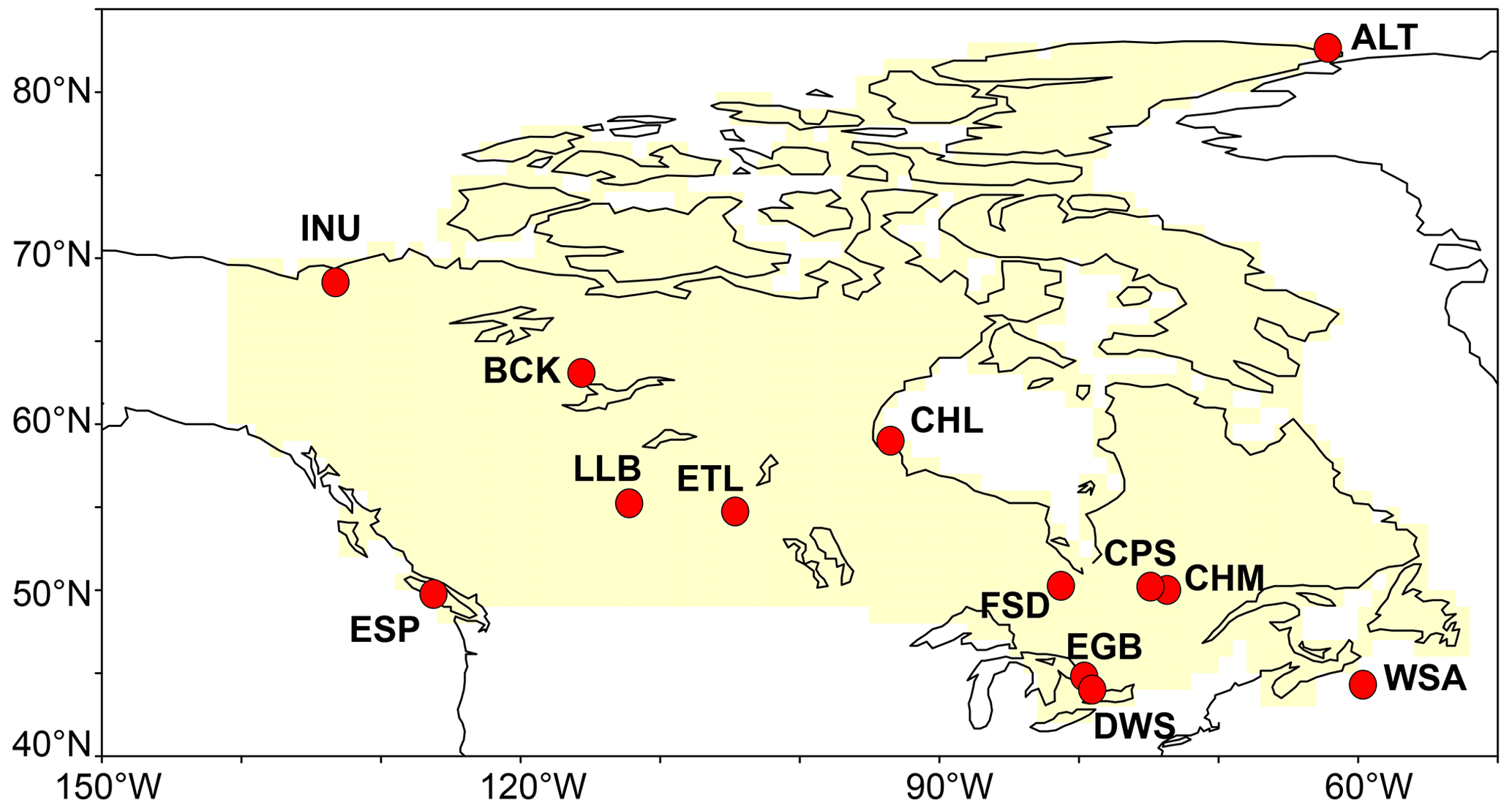
Figure 1The ECCC atmospheric measurement sites used in this study.
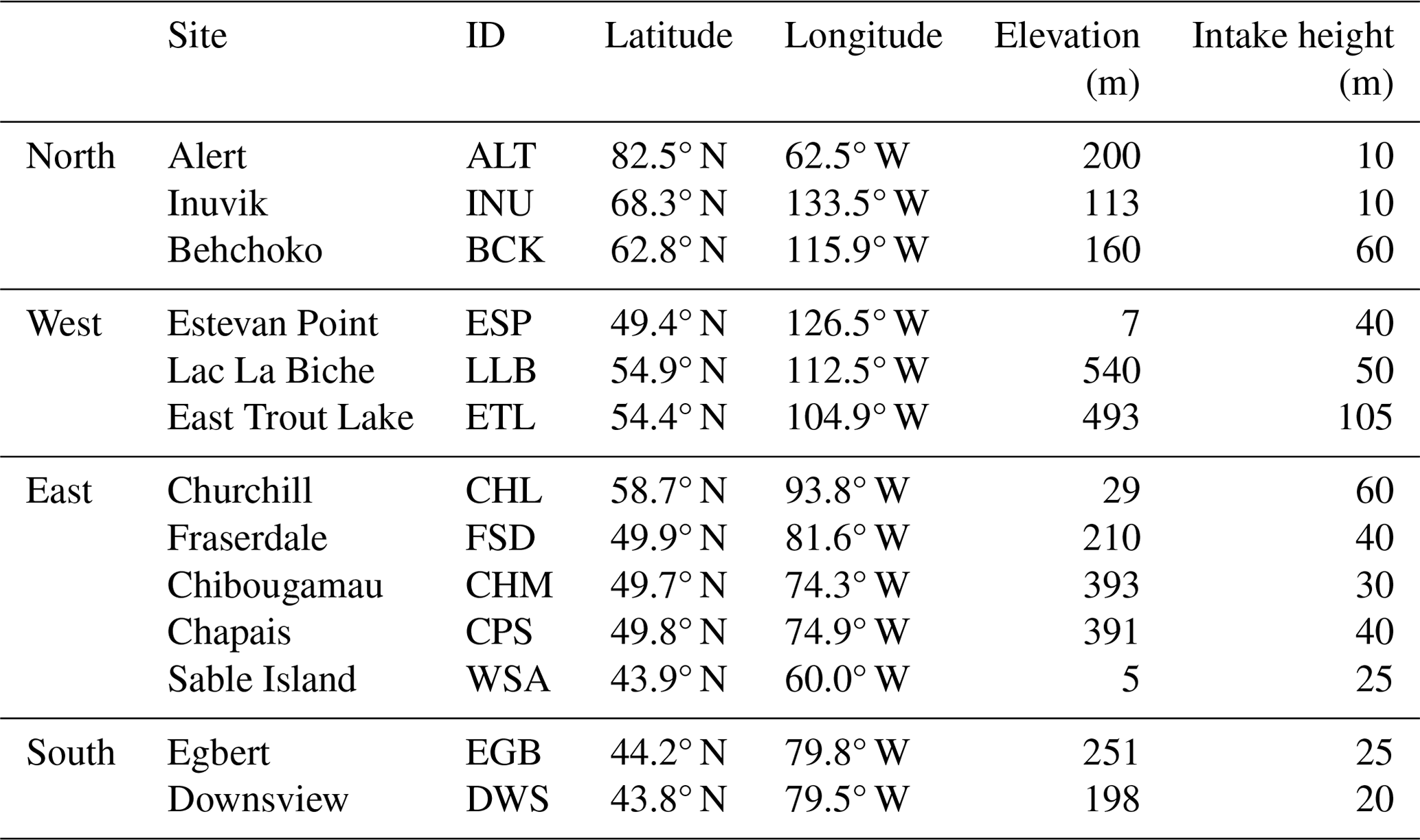
Table 1Measurement sites. North, West, East, and South indicate the four subregions defined in Sect. 2.2.4 (see Fig. 4a).
2.1 Atmospheric CH4 measurements
This study utilized the records of continuous atmospheric CH4 measurements by ECCC's GHG monitoring program across Canada. Among the ECCC-operated sites, we focused on 13 sites (Fig. 1) to constrain Canada's national and subregional CH4 fluxes for 11 years from 2007 to 2017. The chosen sites have records of at least 5 years. The location information of the sites used in this study is in Table 1. Brief descriptions of the sites are provided below, as the detailed descriptions are in the Supplement (Sect. S1).
The ECCC continuous measurement of atmospheric CH4 started in the late 1980s at Alert Observatory (ALT; 82.5° N, 62.5° W) in 1987, followed by the measurement at Fraserdale (FSD; 49.9° N, 81.6° W) in 1989. Alert was established to monitor the baseline GHG for the pan-Arctic region, while Fraserdale has been monitoring CO2 and CH4 in the northern wetlands and boreal forest ecosystems. In the 2000s, the ECCC measurement program was gradually expanded from the west to the east across Canada: Estevan Point (ESP; 49.4° N, 126.5° W) on the Pacific coast; the continental sites Lac La Biche (LLB; 54.9° N, 112.5° W), East Trout Lake (ETL; 54.4° N, 104.9° W), Egbert (EGB; 44.2° N, 79.8° W), Chibougamau (CHM; 49.7° N, 74.3° W), and Chapais (CPS; 49.8° N, 74.9° W; a later replacement for Chibougamau); and Sable Island (WSA; 43.9° N, 60.0° W) off the Atlantic coast. In the 2010s, the observation network was further expanded to the subarctic region in northern Canada – Inuvik (INU; 68.3° N, 133.5° W), Behchoko (BCK; 62.8° N, 115.9° W), and Churchill (CHL; 58.7° N, 93.8° W) – and also to populated areas of southern Canada – Downsview (DWS; 43.8° N, 79.5° W) in Toronto.
Atmospheric CH4 measurements were initially made using a gas chromatograph (GC; Hewlett Packard HP5890 or HP6890) with flame ionization detection (FID). From 2013 onward, GC systems were gradually replaced with cavity ring-down spectrometers (CRDSs; Picarro G1301, G2301, or G2401). All measurements are traceable to the World Meteorological Organization X2004 scale (Dlugokencky et al., 2005). A detailed description of the CH4 measurement system can be found elsewhere (e.g., Chan et al., 2020).
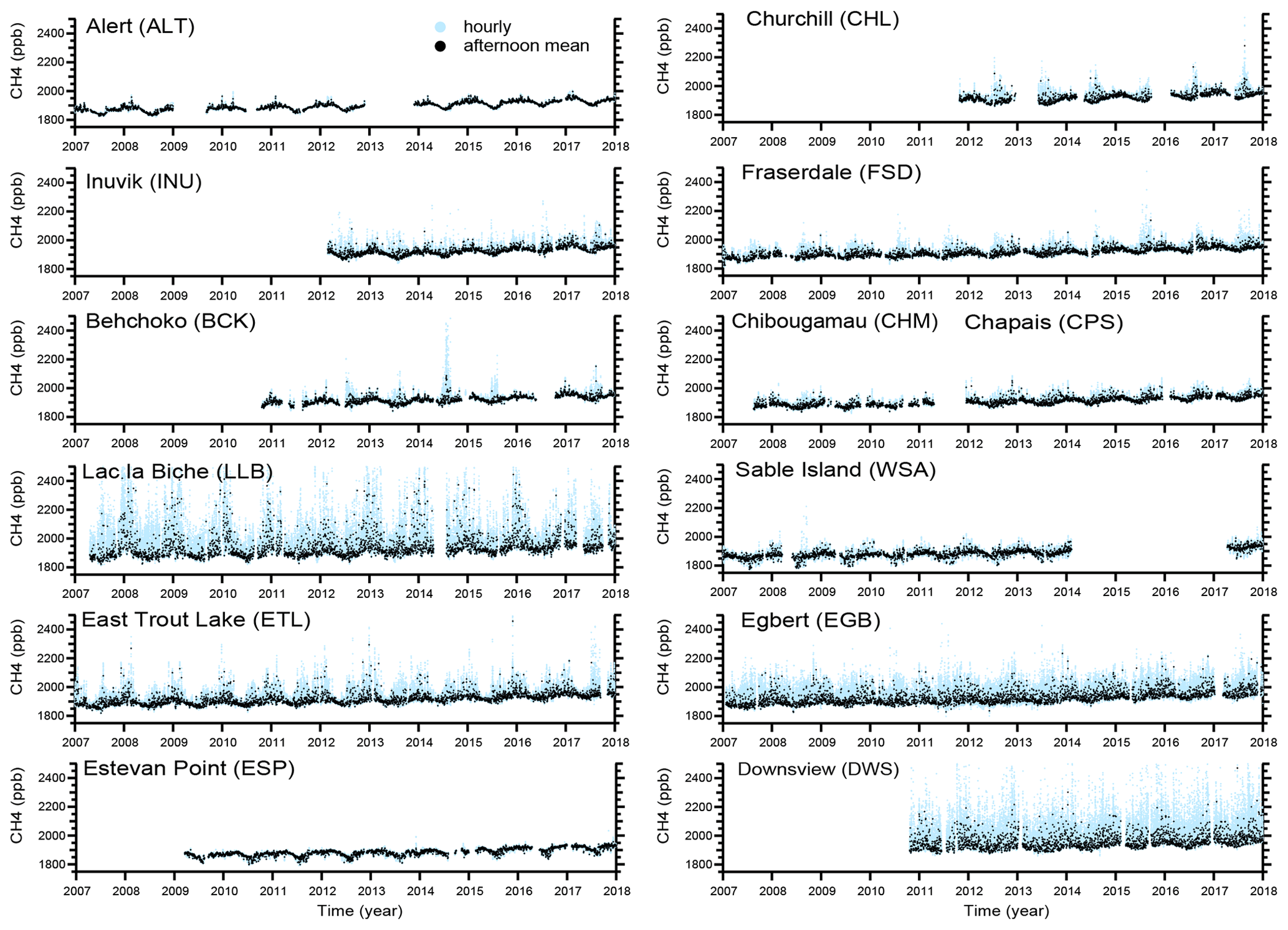
Figure 2Time series of atmospheric CH4 mixing ratios at Canadian sites. The observed values are shown as the hourly means (light blue dot) and afternoon mean (black dot, 12:00–16:00 LT, local time) from continuous measurements.
After the initial quality control, all the atmospheric CH4 measurements are reduced to hourly mean values. To minimize the impact of local-scale variations in atmospheric CH4 on the regional-scale CH4 flux estimates, the hourly data are averaged to afternoon means (from 12:00 to 16:00 LT, local time), assuming midday air is in a well-mixed planetary boundary condition. Then, a curve-fitting method is applied to the time series to remove the outliers from the measurements, which indicate contamination sources probably from sporadic strong local fugitive emissions or issues related to air sampling or analysis. Less than 2 % of the data were removed through this process. The curve-fitting method has two harmonics of 1-year and 6-month cycles and two low- and high-pass digital filters with cut-off periods of 4 and 24 months (Nakazawa et al., 1997). The threshold of outliers is set to be 3 times the standard deviation of the residual of the best-fit curves. Figure 2 shows the hourly and afternoon mean atmospheric CH4 time series at the 13 measurement sites. The respective time series show different variations, reflecting their local and subregional CH4 source strengths.
2.2 Regional inverse model
In this study, we used the Bayesian inversion approach to estimate the regional CH4 fluxes over Canada. The same inverse modelling framework was previously used for CH4 flux estimation in the Canadian Arctic (Ishizawa et al., 2019). The Bayesian inversion optimizes fluxes to minimize the differences between the observations and the modelled atmospheric CH4 mixing ratios. This study calculated modelled CH4 mixing ratios based on the backward runs of Lagrangian particle dispersion models (LPDMs). The optimized flux uncertainties from modelling errors were estimated from an ensemble of 24 inversion experiments using multiple transport models and prior flux estimates. The following sections describe the regional inverse model.
2.2.1 Regional inversion
The Bayesian inversion optimizes the scaling factors of posterior fluxes by minimizing the mismatch between modelled and observed mixing ratios with constraints and given uncertainties using the cost function (J) minimization method (Lin et al., 2004):
where y (N × 1) is the vector of observations (to be comparable to the modelled CH4 (denoted as Kλ) based on the prior fluxes, the background mixing ratio representing the CH4 signal from 5 d prior to the observation time has been subtracted from the observed mixing ratios; see the following Sect. 2.2.2). N is the number of observation points times number of stations (N is for 1 month in our case and is reduced if observations are missing). λ (R × 1) is the vector of the posterior scaling factors to be estimated, and R is the number of subregions to be solved. λprior is the vector of the prior scaling factors which are all initialized to 1 for subregions, and K (N × R) is the matrix of contributions from R subregions. K is a Jacobian matrix of flux sensitivity, a product of two matrices: M and x. M is the modelled transport (or footprints in this study), and x is the spatial distribution of the surface fluxes. A linear regularization term has been added, which is the second term on the right-hand side of the equation. Dϵ and Dprior are the error covariance matrices. Dϵ is the prior model–observation error/uncertainty matrix (N × N), where the diagonal elements are (σe)2. Dprior is the prior scaling factor uncertainty matrix (R × R), where the diagonal elements are (σprior)2. The model–observation mismatch errors are treated as uncorrelated to each other, and the contributions from the subregions are also uncorrelated. All the off-diagonal elements in Dϵ and Dprior are assumed to be zero. We assigned σe = 0.33 (uncertainty of 33 %) for the model–observation error (Gerbig et al., 2003; Lin et al., 2004; Zhao et al., 2009) and σprior = 0.30 (uncertainty of 30 %) for the prior uncertainty (Zhao et al., 2009), as examined in Ishizawa et al. (2019). The inversion's sensitivity to these uncertainties was examined by doubling their values. The results show the optimized fluxes are not strongly dependent on these prescribed uncertainties. The estimate for λ is calculated according to the expression below (Lin et al., 2004):
The posterior error covariance matrix, Σpost, for the estimates of λ is calculated as follows:
We optimize the total CH4 fluxes, including all the CH4 fluxes, on a monthly time resolution.
2.2.2 Atmospheric models
In an LPDM, air-following particles travel backward from the measurement location at a given initiation time (corresponding to the time of observation) and provide the relationship between surface fluxes and atmospheric mixing. This relationship is called footprint, source–receptor relationship, or flux sensitivity. To estimate the transport model errors in the flux estimate, three different models were employed in this study, combining two different LPDMs – FLEXible PARTicle dispersion model (FLEXPART) (Stohl et al., 2005) and Stochastic Time-Inverted Lagrangian Transport Model (STILT) (Lin et al., 2003; Lin and Gerbig, 2005) – and three different meteorological datasets. These three model setups are here named FLEXPART_EI, FLEXPART_JRA55, and WRF-STILT. FLEXPART_EI is FLEXPART v8.2 driven by the European Centre for Medium-Range Weather Forecasts (ECMWF) ERA-Interim (Dee et al., 2011; Uppala et al., 2005), FLEXPART_JRA55 is FLEXPART v8.0 driven by the Japanese 55-year Reanalysis (JRA-55) from the Japanese Meteorological Agency (JMA) (Kobayashi et al., 2015), and WRF-STILT is STILT driven by the Weather Research and Forecasting (WRF) model (e.g., Hu et al., 2019). The WRF-STILT footprints used in this study were provided by the NOAA CarbonTracker-Lagrange project (CT-L; https://gml.noaa.gov/ccgg/carbontracker-lagrange, last access: 10 September 2023). All the footprints calculated by the respective models were mapped onto 1.0° × 1.0° grids.
LPDMs simulate surface contributions for a certain period prior to the measurements at sites by air-following particles. In this study, at the endpoints of the particles after 5 d back-trajectory, the background conditions of atmospheric CH4 mixing ratios were provided by a global model, the National Institute for Environmental Studies Transport Model (NIES TM), with optimized global CH4 flux fields by the GELCA-CH4 inverse model (Ishizawa et al., 2016). The performance of NIES TM simulation with GELCA-CH4 optimized fluxes was reported in Chan et al. (2020).
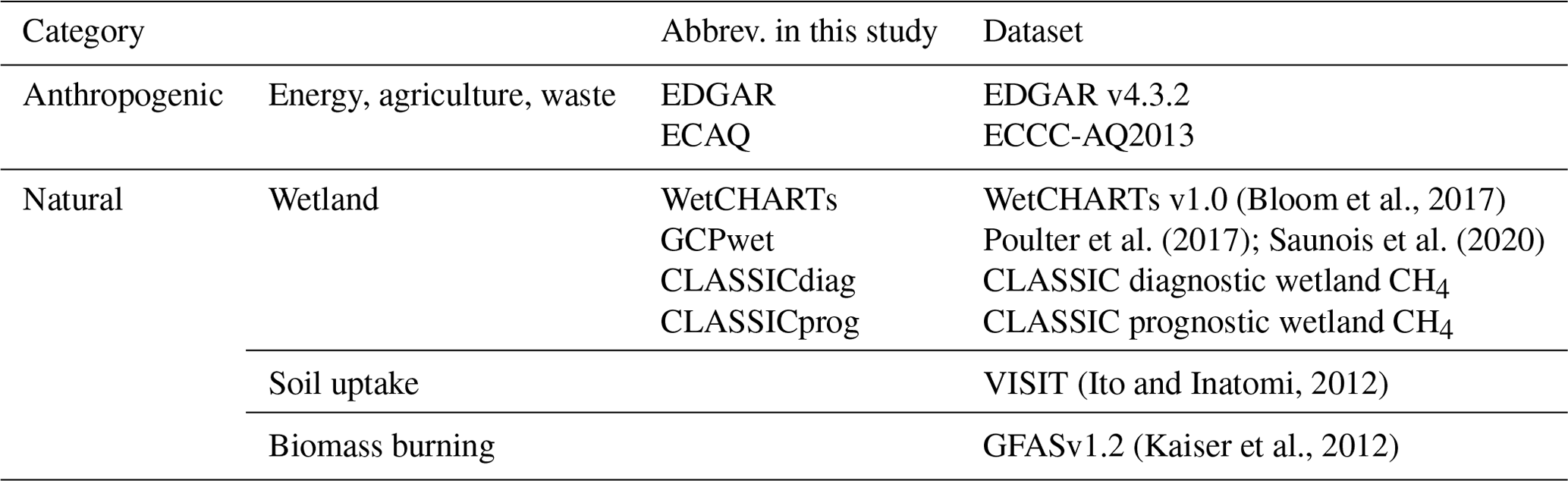
Table 2Prior fluxes used in this study. Eight prior flux scenarios were made as combinations of two anthropogenic fluxes (EDGAR and ECAQ) and four wetland fluxes (WetCHARTs, GCPwet, CLASSICdiag, and CLASSICprog). For other natural fluxes, the same prior datasets were used in all the scenarios.
There are many factors governing the transport-model-simulated concentrations at the measurement sites used in this study, such as the spatial distribution of emissions and meteorological conditions, including winds and atmospheric stability. Since we are focusing on the synoptic variability in our observations, these are the results of the regional emissions (typically within the synoptic spatial scale of ∼ 100–1000 km). This region of interest is covered by the model footprint within the first 3 to 5 d. Another reason for limiting the footprints to 5 d is that footprint uncertainty grows the longer the hindcast or model dispersion is (analogous to forecast uncertainty). Using 5 d footprints in the inversion model is similar to other studies (e.g., Cooper et al., 2010; Gloor et al., 2001; Stohl et al., 2009). These studies have shown that 5 d is typically sufficient to capture the surface influence on a measurement site from the surrounding region. Figure S15a shows the typical footprint strength as a function of days of hindcast. Figure S15b illustrates the differences in simulated concentrations between 5 and 10 d footprints for our measurement sites and how they compare (∼ 10 %) with the much larger differences resulting from using different transport models in this study. Therefore, we used 5 d footprints in our model and included the footprint contribution beyond 5 d implicitly as a part of the background concentration extracted at the 5 d particle endpoint locations. Other inversion studies could optimize emissions far from the observation sites (with weak nearby emissions); it would be necessary to consider footprints from 5 to 10 d or more in such cases, even though the footprint (or model transport) uncertainties could become large (possibly) and lead to correspondingly large uncertainties in the inversion results.
2.2.3 Prior CH4 fluxes
We considered eight scenarios of prior emissions, combining four different wetland fluxes and two anthropogenic emission inventories (Table 2).
The first wetland ensemble model, WetCHARTs, derives wetland CH4 fluxes as a function of a global scaling factor, wetland extent, heterotrophic respiration, and temperature dependence (Bloom et al., 2017). We used the ensemble mean fluxes over 18 model sets available for 2001–2015. The second wetland flux set is the monthly climatological estimates from the ensemble mean of 16 wetland process-based models (Poulter et al., 2017), which was provided for the GCP-CH4 inversion project (Saunois et al., 2020) (GCPwet in short hereinafter). The last two wetland CH4 fluxes are from the Canadian Land Surface Scheme Including Biogeochemical Cycles (CLASSIC), which is a successor to the Canadian Land Surface Scheme (CLASS) and the Canadian Terrestrial Ecosystem Model (CTEM) (Melton et al., 2020). The four sets of CLASSIC wetland CH4 fluxes were calculated with two different meteorological datasets, CRU-JRA (Harris et al., 2020) and GSWP3 (Dirmeyer et al., 2006), which use diagnostically specified and prognostically determined wetland extents. These two different schemes predict different spatial distributions and temporal variations in wetland CH4 emissions. The choice of the meteorological dataset appears to be less influential in simulated CLASSIC CH4 fluxes, indicating that the model response to both meteorological forcings is consistent. Therefore, these four sets were aggregated to the two sets of CLASSIC wetland CH4 fluxes (diagnostic and prognostic wetland extents) by averaging simulated CH4 emissions for the two different meteorological forcing datasets. These diagnostic and prognostic CLASSIC CH4 flux sets are abbreviated as CLASSICdiag and CLASSICprog, respectively. Figure 3a shows the spatial distribution of the four wetland CH4 fluxes for a summer month (July) and a winter month (January). Overall GCPwet shows stronger emissions among the four prior summer wetland fluxes, especially along Hudson Bay and around the border between Northwest Territories and Alberta in western Canada, resulting in approximately doubled annual emissions at subregional and national levels compared to the other estimates (Fig. 3c). GCPwet shows the strongest summer emissions but weaker winter emissions than WetCHARTs and CLASSICdiag, which have noticeable winter emissions. CLASSICprog also shows almost negligible winter emissions, while summertime emissions are stronger than CLASSICdiag (Fig. 3e). Annually the two CLASSIC wetland fluxes, CLASSICdiag and CLASSICprog, have similar annual emissions at the national and subregional levels (Fig. 3c).
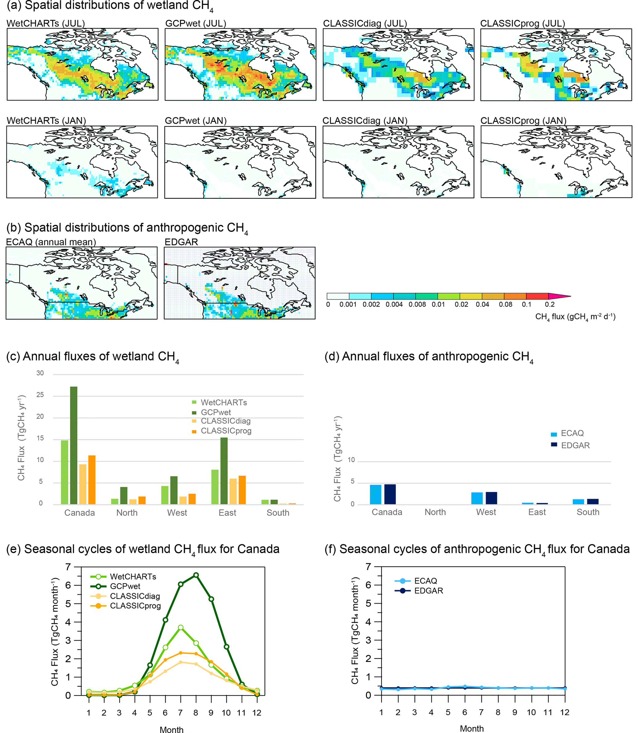
Figure 3Wetland and anthropogenic prior CH4 fluxes in this study. Spatial distributions (a, b) and annual fluxes (c, d) for Canada and subregions and seasonal cycles (e, f) for Canada. The variations in wetland CH4 fluxes are climatological or multiyear means, and those of anthropogenic CH4 fluxes are for 2013. The subregions North, West, East, and South are defined in Sect. 2.2.4 (see Fig. 4a).
The two sets of anthropogenic CH4 emissions used in this study are the monthly ECCC-AQ2013 (ECAQ) scaled to the NIR sectoral totals for the year 2013 by province (Chan et al., 2020) and the annual Emissions Database for Global Atmospheric Research (EDGAR) v4.3.2 (Janssens-Maenhout et al., 2019). As seen in Fig. 3b, Canada's anthropogenic emissions are concentrated around the western provinces and the southern border. The spatial patterns of both prior-emission datasets are quite similar, though there are some differences in hotspot locations (Fig. 3b and d). The seasonal variability in ECAQ is small compared to the variability in wetland fluxes (Fig. 3e and f).
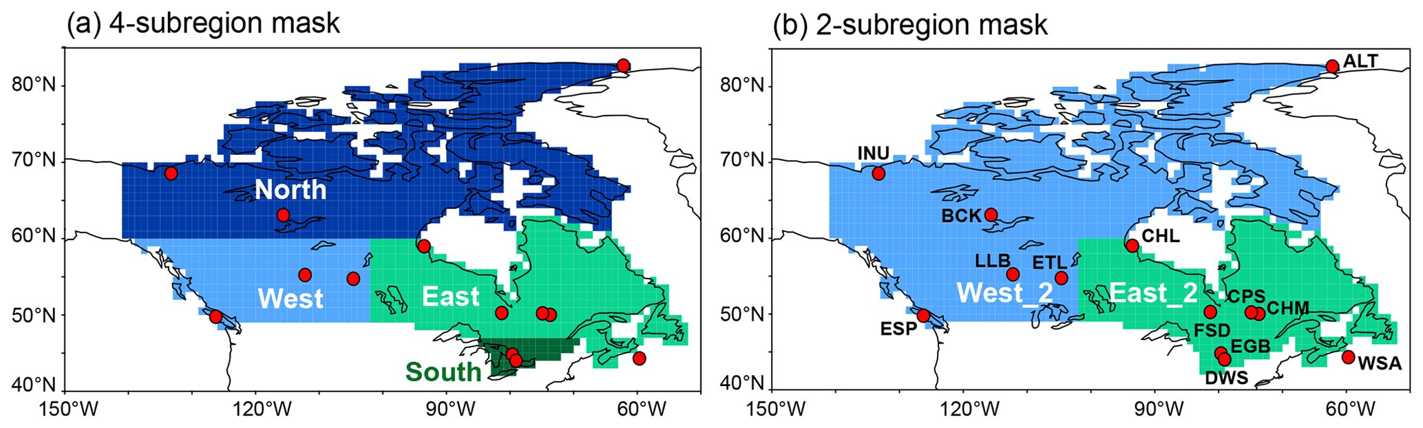
Figure 4Subregion masks for inversion and the ECCC atmospheric measurement sites. Canada is divided into (a) four subregions (North, West, East, and South) and (b) two subregions (West_2, East_2). These subregion masks are based on Canadian provinces and territories (see Fig. S2), climate zones, and industrial activities. The observation sites are also shown.
The CH4 emission estimates for two other categories used in this study are daily biomass burning (BB) emissions from Global Fire Assimilation System (GFAS) v1.2 (Kaiser et al., 2012) and the climatological monthly soil CH4 uptake based on VISIT-CH4 (Ito and Inatomi, 2012). In Canada, the VISIT-modelled soil uptake is weak (−1.6 Tg CH4 yr−1) and widely distributed spatially in the summer months. If the prior data did not cover the whole analysis period, the respective mean values from the last 5 years were repeatedly used afterwards; climatological prior-emission datasets (e.g., GCPwet) were used without further processing. All data are converted into 1.0° × 1.0° grids by simply aggregating finer-spatial-resolution data (e.g., EDGAR) or re-gridding coarser data (e.g., CLASSIC).
2.2.4 Domain and subregions
The regional domain of interest for this study is Canada. We set up two subregion masks for Canada, mainly based upon climate zone with a provincial–territorial division and industrial activities also considered (see Fig. S2 for the Canadian provinces and territories). Outside Canada was treated as one outer region. The first mask consists of four subregions: North, West, East, and South (defined in Fig. 4a). The second mask reduces the four subregions to two: North and West become West_2 and East and South become East_2 (Fig. 4b). The subregion North covers the Canadian Arctic, including Northwest Territories (NT), Yukon (YT), and Nunavut (NU). In North, the major CH4 sources are natural, primarily wetlands and occasionally some biomass burning. The subregion West includes the three western provinces: British Columbia (BC), Alberta (AB), and Saskatchewan (SK). AB and SK are the largest oil and gas CH4 emitting provinces in Canada, which account for ∼ 70 % of the national emissions from the oil and gas sectors (ECCC, 2022). The subregion West has other anthropogenic sources such as the agriculture sector and natural sources, primarily wetlands. The CH4 emission in the subregion East is mainly from natural wetlands, where the Hudson Bay Lowlands (HBL) are located. The subregion South is southern Ontario (ON) and Quebec (QC) (south of 48° N), the most populated area in Canada, resulting in considerable anthropogenic CH4 emissions from energy and agriculture sectors and landfills (waste management).
The sensitivity of the flux estimation to the number of subregions was examined; increasing the spatial resolution to six subregions revealed some model instability problems. With the limited observational constraints during this study period, subregions with weak prior fluxes or lack of measurement sites demonstrated larger uncertainties in estimated fluxes, with frequent unrealistic negative fluxes. Similar relations in resolving power of inversions were reported in Ishizawa et al. (2019) and Chan et al. (2020). Therefore, this study focuses on the inversion results of the four subregions and the two larger subregions.
In our model testing, the statistical Bayesian inversion model worked well if the basic model assumptions were satisfied. The important assumptions are (1) no transport errors and (2) a large dataset for robust statistics. We found that the main reason for the negative posterior fluxes in our model is transport errors (the inversion model yields the best statistical fit of the observations without accounting for transport biases). For atmospheric transport with random errors (unbiased), the model still works well if there are sufficient constraining data (“observations”) to allow the statistical model to robustly estimate the scaling factors. Imposing positive flux constraints (usually for negative solutions resulting from a scarcity of constraining data; e.g., Michalak and Kitanidis, 2003) does not appear to address the problem of transport biases. Positive flux constraints or imposing non-negativity constraints on the scaling factors could violate the statistical assumptions in our linear Bayesian inverse model, namely linearity and normality.
There are inversion studies doing grid-scale inversions (using non-zero off-diagonal covariance constraints) to address the aggregation error issue (e.g., Gourdji et al., 2012; Hu et al., 2019; Thompson et al., 2017). These grid-scale inversions are limited by the lack of observations and systematic transport errors (Gourdji et al., 2012). Their discussions about them are typically on the aggregated fluxes in larger regions and temporally averaged estimated features. This is consistent with our inversion model sensitivity analysis; we found that inversion flux errors from the transport model errors appear larger than aggregation errors in our case. For example, in the worst-case scenario, the difference of the inversion results calculated by different transport models could be greater than 100 %.
In this study, we tried to reduce the effects of transport model biases and insufficient observations for statistical Bayesian inversion analysis. We used multiple transport models to lessen the effects of individual transport model biases and to provide flux uncertainty estimates associated with the choice of transport model. This inversion model employed a limited number of subregions to allow the abundant observations to provide sufficient constraints to obtain flux estimates that appear robust and positive without the added model complications like positivity constraints and non-zero off-diagonal covariance constraints.
Flux estimations by inversion models can be complex: the flux estimate uncertainties depend on the tracer bio-geochemical characteristics; quantity and quality of the observations; and model formulation, setup, and assumptions. Having a wide range of models (including grid point inversion, non-negative constrained inversion, and multi-transport with abundant observational constraint inversion used here) could be helpful in understanding the strengths and weaknesses of inversion modelling.
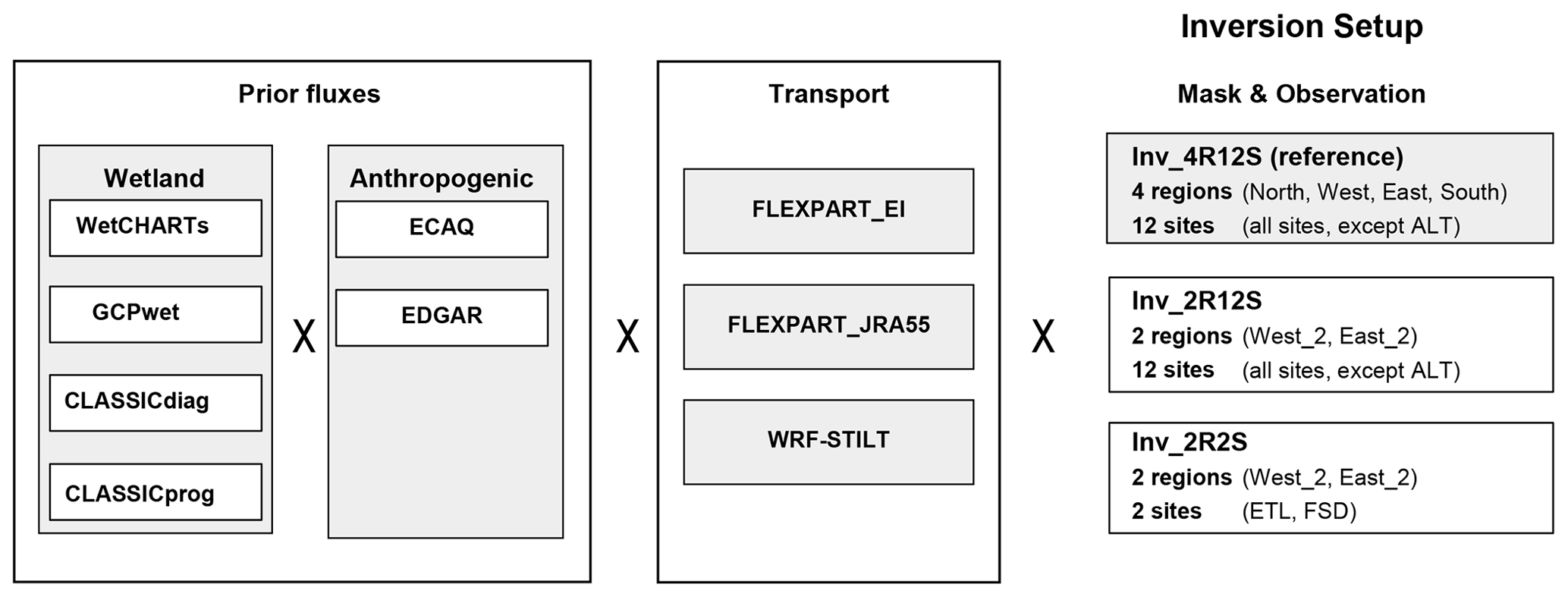
Figure 5Diagram of inversion experiment settings in this study. Eight prior-emission scenarios out of four wetland fluxes and two anthropogenic fluxes are applied to three different transport models. These flux–transport combinations yield the 24 experiments as listed in Table S1. The experiments with a 4-subregion mask and 12 observation sites are conducted as the reference inversion (Inv_4R12S). The experiments with a 2-subregion mask and 12 observation sites (Inv_2R12S) or 2 sites (Inv_2R2S) are performed as additional inversions. The mask maps are defined in Fig. 4, along with observation site locations.
2.2.5 Experimental setup
Figure 5 shows the schematic diagram of the inversion experiments regarding the combinations of prior fluxes, transport models, subregion masks, and observations. The ensemble of 24 experiments consists of the permutations of eight prior flux scenarios and three transport models, as summarized in Table S1 in the Supplement. It is noted that the maximum number of observation sites was 12 in this inversion, as Alert (ALT) was not used for the flux estimation. The marine boundary layer site ALT at the northern end of the subregion North appears not to see the subregional flux signals (mainly in the southern part of the subregion) above the background atmospheric CH4 (Ishizawa et al., 2019). Therefore, ALT was not included in the inversion of this study, following the inversion study of Canadian Arctic CH4 (Ishizawa et al., 2019). As the reference inversion, we performed these 24 experiments with the 4-subregion mask and all 12 site observations (abbreviated as Inv_4R12S). As a sensitivity test to examine the impact of observational coverage, two additional inversions using the 2-subregion mask with the 12 sites (Inv_2R12S) and the 2 sites of ETL and FSD (Inv_2R2S) were conducted with the same ensemble setup of 24 experiments. ETL and FSD have long measurement records extending back beyond the period of this study. Therefore, the inversion Inv_2R2S explored the feasibility of estimating CH4 fluxes by inversion for a longer time period.
2.3 Partition into natural fluxes and anthropogenic fluxes
The posterior CH4 flux in this study is the total flux (natural plus anthropogenic). Thus, we need a scheme with assumptions to partition the total fluxes into natural and anthropogenic sources. Some previous studies for the northern extra-tropical region (e.g., Tohjima et al., 2014; Thompson et al., 2017) estimated the anthropogenic sources by assuming that, in the winter season, anthropogenic CH4 fluxes are dominant, while biogenic CH4 fluxes (e.g., natural wetlands or rice cultivation) are dormant and negligible. This assumption is consistent with many process-based wetland models, as demonstrated by the prior wetland fluxes used in this study (see Fig. 3e). In this study, the prior wetland CH4 winter flux fraction (November to March, < 60° N) to the annual emissions in Canada is in the range of 2.6 % to 9.2 %.
Here, considering the possible winter wetland CH4 emissions in the flux partition, we applied the following simple scheme to partition natural fluxes into warm (growing) and cold (non-growing) seasons, with the assumption of temporally uniform anthropogenic emissions. Let ftotal(m) be the monthly posterior total flux and Ftotal be the annual total flux. Then, Ftotal consists of annual natural and anthropogenic fluxes (Fnatural, Fanthropogenic), and the annual total flux could also be expressed as the sums of monthly total fluxes in the warm season (Ftotal_warm) and the cold season (Ftotal_cold):
Next, these annual fluxes could be expanded in terms of the fraction, Rcold, of the cold season's natural CH4 emissions to its annual emissions and the number of cold months, Ncold, as in Eqs. (6) and (7):
where
If Rcold and Ncold for each subregion are given, the annual fluxes of natural and anthropogenic sources, Fnatural and Fanthropogenic, can be solved through Eqs. (6) and (7). We define the cold (non-growing) season as November to March for all the subregions (< 60° N), except from October to May for North (Canadian Arctic; > 60° N), following Treat et al. (2018). The cold season approximates the period when the air temperature is below 0 °C, as seen in Fig. 10. The estimation of Rcold is explained in Sect. 3.5.2.
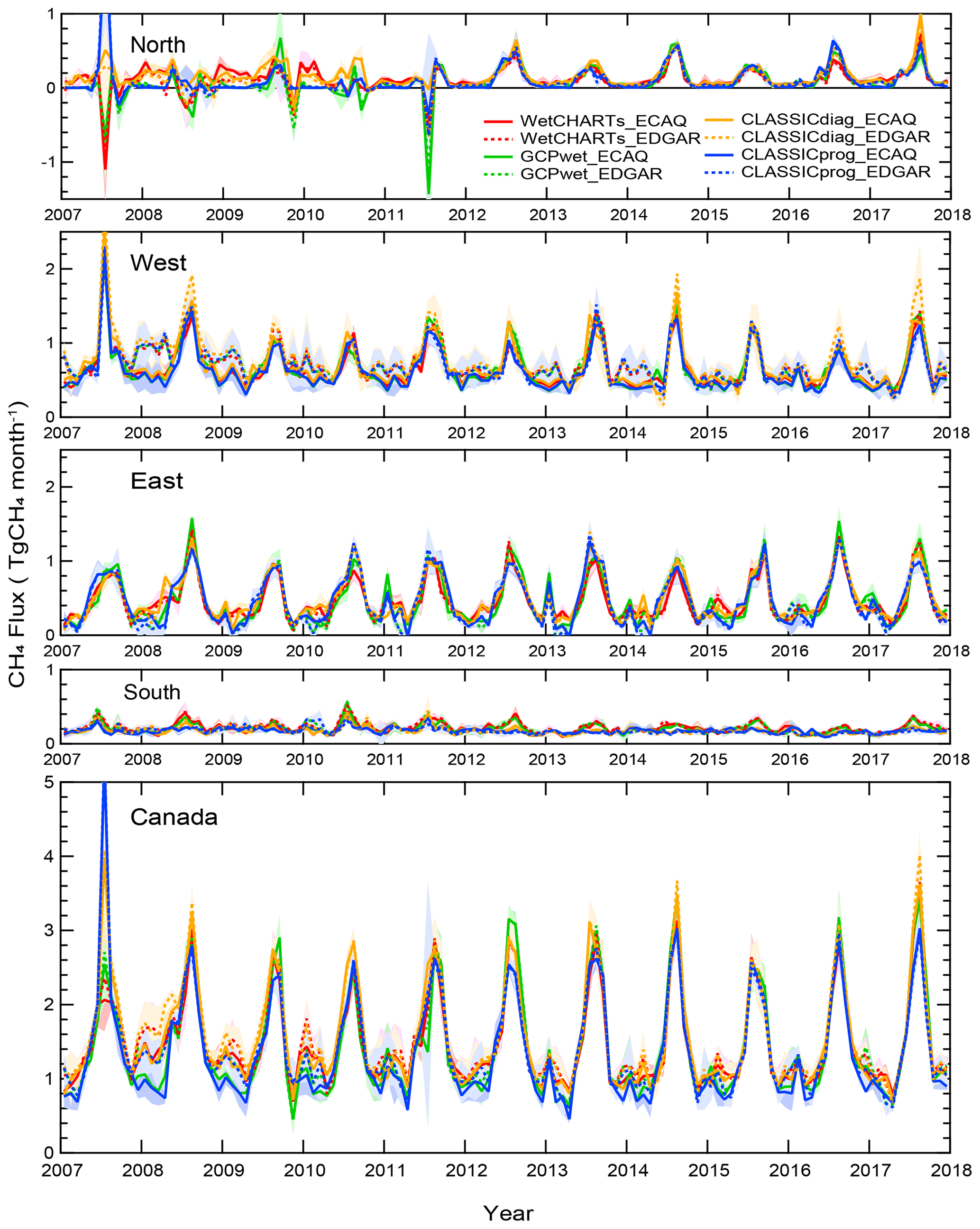
Figure 6Monthly posterior CH4 fluxes for subregions and Canada in the reference inversion Inv_4R12S. The lines are the mean posterior fluxes of experiments with three transport models (FLEXPART_EI, FLEXPART_JRA55, and WRF-STILT) per prior flux scenario. The eight prior flux scenarios are used: WetCHARTs_ECAQ (solid red), WetCHARTs_EDGAR (dotted red), GCPwet_ECAQ (solid green), GCPwet_EDGAR (dotted green), CLASSICdiag_ECAQ (solid orange), CLASSICdiag_EDGAR (dotted orange), CLASSICprog_ECAQ (solid blue), and CLASSICprog_EDGAR (dotted blue). The respective shaded areas indicate the range of minimum and maximum estimates.
3.1 Estimated monthly CH4 fluxes
The monthly posterior CH4 fluxes from 2007 to 2017 for the four subregions and national total are shown in Figs. 6 and S3. The posterior fluxes during the early period from 2007 to 2011 are highly variable, most notably in North, with posterior fluxes showing unrealistic negative fluxes, indicating they are not constrained by the inverse model. Before 2012, the subregion North did not have sufficient observations to constrain the inverse model (see Fig. 4a). Similarly, the measurement sites far to the south (e.g., Lac La Biche (LLB) and East Trout Lake (ETL) in West) also could not constrain the fluxes in North; the stronger flux signals in West tend to mask the signals from North. In October 2010, the site Behchoko (BCK) in the southern part of North began measurements. However, the presence of data gaps still likely resulted in negative fluxes in North for 2011. From 2012 onward, BCK, along with the new sites Inuvik (INU) and Churchill (CHL), provided sufficient constraints on North to yield positive (more reasonable) posterior fluxes with a summer maximum in the seasonal cycle from the wetland CH4 fluxes.
The subregion West (on the south side of the subregion North; see Fig. 4a) also shows more variability in the posterior fluxes before 2012, particularly in the 2008 and 2010 winters. The presence of the poorly constrained North before 2012 (an extra degree of freedom in the inversion) appears to influence the statistical optimization of the inverse model as a whole, leading to more temporal variability and larger posterior uncertainties in the posterior fluxes in West. As noted from 2012 onward, there appear to be sufficient sites and observations to constrain North. Consequently, the posterior fluxes for West also show less variability and a reduction in the posterior uncertainties or more robustness after 2012.
Figure 6 also shows the variability in the seasonal cycle of posterior fluxes among the inversions and the inter-annual variability in the magnitudes, particularly in the summer maxima in the different subregions. Section 3.4.1 discusses the variability in the seasonal cycle of the fluxes among the different inversion settings, as well as the ensemble mean seasonal cycles for subregions. The inter-annual variation in summer wetland fluxes and the relationship to meteorological conditions are examined in Sect. 3.4.2.
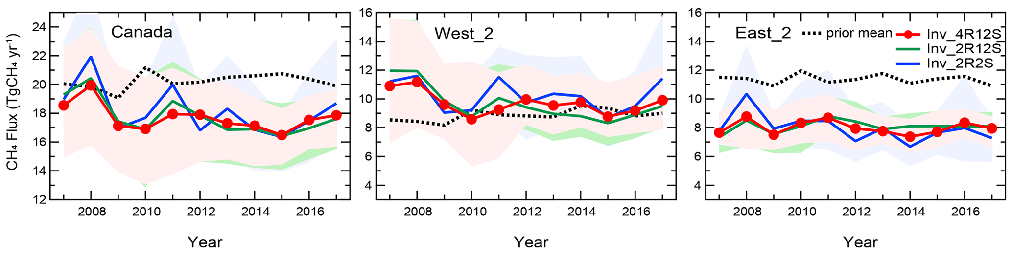
Figure 7Trend of estimated yearly CH4 fluxes in Canada and western (West_2) and eastern (East_2) subregions from three inversion setups (72 experiments in total). Lines show mean fluxes over each of the three inversion sets with different subregion masks and observation site selections. The shaded areas indicate the range of maximum and minimum estimates among 24 experiments per inversion setup. Dotted black lines indicate mean prior emissions.
3.2 Trend of annual mean fluxes
In Sect. 3.1, the inversion results with 4 subregions and 12 observation sites (reference inversion Inv_4R12S) show large temporal variability and uncertainties for the posterior CH4 fluxes for some subregions in the early period (2007–2011) compared to the later period. The potentially poorly constrained fluxes could affect the trends in the results. Thus, we performed the two additional inversions with different settings. The first inversion (Inv_2R12S) used two subregions (West_2 and East_2 in Fig. 4b) and constrained the fluxes with the same set of observations as the reference inversion (Inv_4R12S); the second inversion (Inv_2R2S) used the same two subregions and constrained the fluxes by the two measurement sites ETL and FSD. The advantage of using fewer subregions is having more observations per subregion to constrain the fluxes; the disadvantage is the inability to estimate the possible differences within each subregion. These inversions measure the stability or robustness (to changing setups) of the inversion results, including the possible trend. The sites ETL and FSD are the sites that have the longest records in the mainland of Canada, covering the entire period of this study. As ETL and FSD are located in western and eastern Canada, respectively, these two sites could potentially constrain the subregions West_2 and East_2, respectively. The respective and combined footprints for ETL and FSD are shown in Fig. S4.
To investigate the presence of trends over 2007–2017, the mean annual posterior CH4 fluxes (ensemble means of 24 experiments per inversion setup as described in Fig. 5) are shown for all of Canada and two large subregions (West_2 and East_2) from the three inversion setups (Inv_4R12S, Inv_2R12S, and Inv_2R2S) together in Fig. 7. Figure S5 shows the mean annual posterior CH4 fluxes by prior flux scenario per inversion setup. For the whole inversion period from 2007 to 2017, these three inversions agree within the range of results among the 24 experiments per inversion setup (shown as the shaded bands) for Canada and the two large subregions. For the later period with more observational coverage (2012–2017), the three inversions are in better agreement. Thus, the estimated fluxes appear robust regarding the different setups used for the whole period. However, the variability in the inversion results or shaded bands appears larger in the beginning period when the observational coverage was limited. In addition, the inversion Inv_2R2S has larger inter-annual variability than the inversions constrained by 12 sites. This is consistent with the statistical nature of the Bayesian inversion; statistical inferences are generally better with larger samples of data or observations.
Comparing all the inversion results for long-term trends for the 11 years (Fig. 7), there is no consistent trend for Canada and the two subregions. The mean trend slopes and uncertainties are shown in Table S2. The inversion Inv_2R2S shows a slight downward trend in East_2, but the trend is within the inter-annual variability in the estimated fluxes. This possible trend is not replicated in the other two inversion setups using 12 observation sites (Inv_4R12S and Inv_2R12S). The apparent trend may be due to insufficient observations (making the results sensitive to missing observations) to statistically constrain the fluxes. As shown in Fig. S1 in the Supplement, the data availability at FSD is low (< 10 per month) for 4 months, March to June 2008, possibly resulting in less-constrained fluxes for East_2 in Inv_2R2S. In the inversions using 12 observation sites (Inv_4R12S and Inv_2R12S), CHM, which is ∼ 500 km east of FSD, provides full observational constraints for those 4 months. Another caveat in trend analysis for subregions is exhibited in Fig. S6 for Inv_4R12S. With the four subregions, the subregions North and West (equivalent to West_2) are showing upward and downward trends, respectively, which is possibly another signal of the lack of observational constraints in the early period noted above. There are opposite trends in North and West, resulting in the absence of a trend (not a statistically significant trend) for the combined subregion West_2, as shown in Figs. 7 and S6 and Table S2. This result indicates that sparse data coverage could yield spurious trends on the subregional scale from top-down analysis.
Our result of no significant long-term trend for the national total CH4 emissions during the period 2007–2017 contrasts with some other studies showing possible trends. For example, Thompson et al. (2017), from the 9-year inversion for 2005–2013, concluded that there was a positive trend in CH4 emissions in northern America (> 50° N, Canada and Alaska) of 0.38 to 0.57 Tg CH4 yr−2, especially in the HBL due to warming soil temperature. The ensemble mean of GCP-CH4 global inversions showed a gradual downward trend over the last 2 decades of 2000–2017 (Stavert et al., 2021), which is attributed to a reduction in wetland emissions of ∼ −0.3 Tg CH4 yr−2. However, the inferred downward trend does not agree with the ensemble of the process-based wetland model estimate; all the wetland models show an upward trend (Stavert et al., 2021). These contrasting results point to the difficulty of inferring long-term trends from highly variable data and insufficient data coverage for Canada. Thus, continuous atmospheric CH4 measurements with good spatial coverage are needed to detect any long-term changes in CH4 emissions in response to climate forcings or anthropogenic emission changes.
3.3 Evaluation of posterior fluxes
A model–data comparison of atmospheric mixing ratios at the measurement sites is commonly employed to evaluate the posterior fluxes. Figure S7 shows the model–data comparison by measuring the mean biases and correlation coefficients between the simulated and observed mixing ratios at each site in all 24 experiments for the reference inversion Inv_4R12S. The results of the simulated prior mixing ratios are overall dependent on the prior fluxes and transport models. The simulated posterior mixing ratios show an improvement in matching with the observations at most of the sites, except ESP. Also, DWS exhibits a notable transport model dependency. The FLEXPART_JRA55 cases show larger biases than the other transport model cases. This might be related to the resolution of the driving meteorological data of FLEXPART_JRA55 (1.25° × 1.25° horizontal resolution and 6-hourly time step) as opposed to other models (1.0° × 1.0° and 3-hourly time step in FLEXPART_EI and 10 km × 10 km and 1-hourly time step in WRF-STILT), which might be too coarse to model the urban site DWS. The correlations between the posterior mixing ratios and the observations are improved, being around 0.9 at all the sites. The correlation at ESP is unchanged after the inversion. This indicates that ESP, which is the most western site on the Pacific coast in Canada, has already been simulated well by the background mixing ratios and is not strongly influenced by the continental fluxes. On the other side of the continent, the most eastern site WSA, on Sable Island in the Atlantic, shows a slight improvement after the inversion.
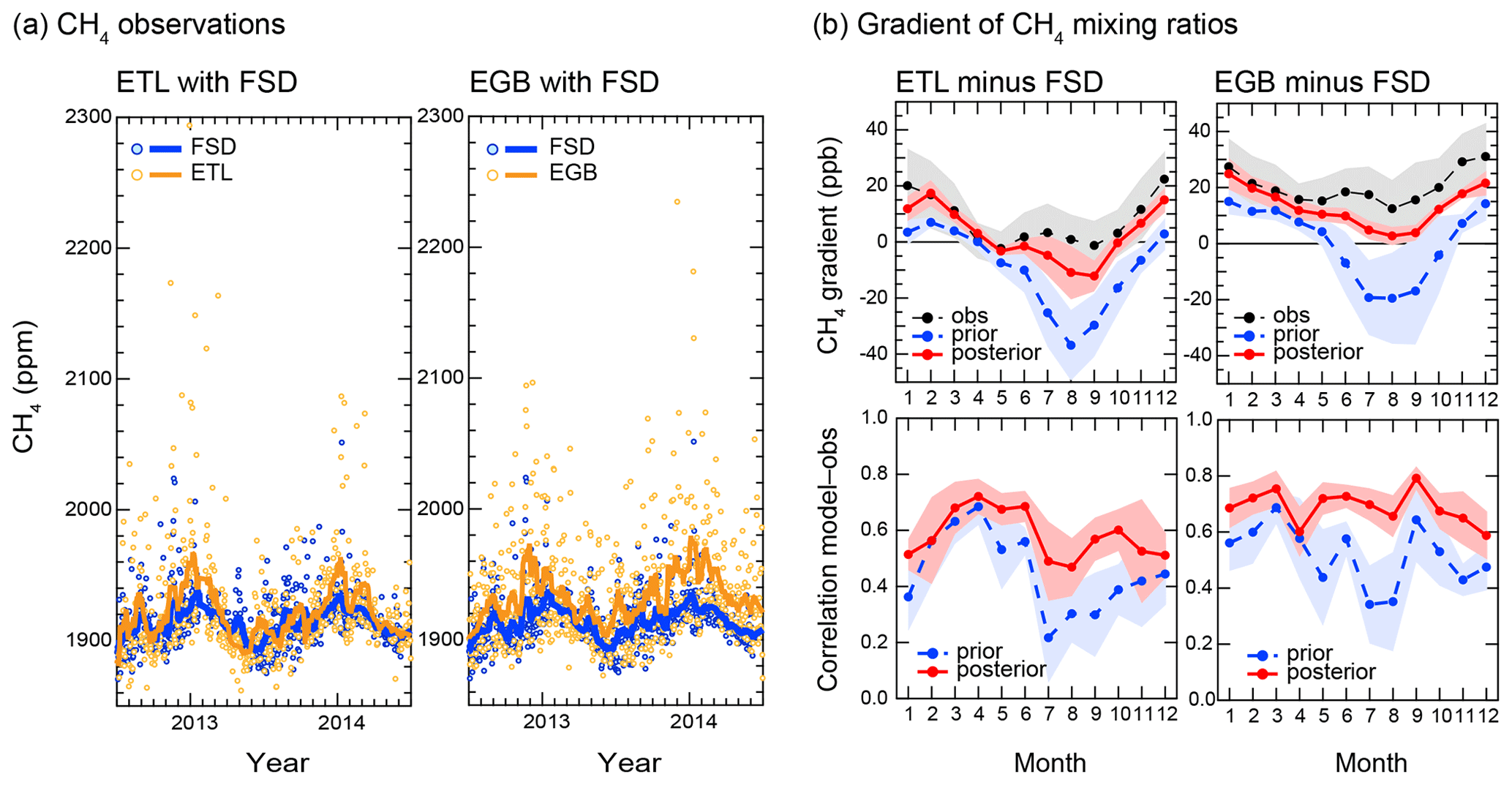
Figure 8(a) Examples of time series of CH4 mixing ratios observed at ETL and EGB, along with the CH4 mixing ratios at FSD. The circles are afternoon means, and solid lines are smoothed curves with a 20 d moving window average. (b) Gradients of the mixing ratio between ETL and FSD and between EGB and FSD (top) and the correlation (bottom). In the top, solid red lines with markers are the mean gradients of modelled CH4 mixing ratios with posterior fluxes over 2012–2017, and dotted blue lines with markers are the modelled gradients with prior fluxes. Black lines with markers are mean gradients of observed CH4 mixing ratios. At the bottom, red lines show the mean correlation between the modelled posterior gradient and observations, and blue lines show the correlations between the modelled prior gradient and observations.
In this study, we explored another type of data for posterior flux evaluation. There is flux information in the observed mixing ratio difference (or gradient) between sites. Fan et al. (1998) noted that the downwind and upwind mixing ratios' difference for a given region should reflect the source/sink strength within the region. For example, for CO2 uptake of 1.7 Gt C yr−1 over North America, there could be an annual difference of ∼ 0.3 ppm from the Atlantic coast to the Pacific coast. Such small differences are challenging to extract, given the large variability in the atmospheric CO2 mixing ratios. However, on smaller spatiotemporal scales (mesoscale to microscale), local or urban emission studies (e.g., Bréon et al., 2015; Mitchell et al., 2018) and large-point-source estimates from satellites (e.g., Nassar et al., 2022) have used mixing ratio differences to constrain city-scale or facility-scale emissions. Thus, the following examines the relationship between mixing ratio difference and regional fluxes on the larger (synoptic) scales of this study.
For the case of the mixing ratio difference (ΔCETL−FSD = CETL−CFSD) between East Trout Lake (ETL) and Fraserdale (FSD), which are ∼ 2600 km apart and approximately along the prevailing westerly wind direction, there are no consistent correlations between ΔCETL−FSD and CETL or between ΔCETL−FSD and CFSD (see Fig. S8). As the uncorrelated information in ΔCETL−FSD has not been used to constrain the inverse model, ΔCETL−FSD could serve as an evaluation of the inversion results. The comparison of multiyear (2012–2017) averaged monthly mixing ratio difference between models and observations is shown in Fig. 8. In addition to comparing the east–west difference (ΔCETL−FRD between ETL and FSD), the north–south difference (ΔCEGB−FRD = CETL−CFSD) between Egbert (EGB) and FSD is also compared in Fig. 8. The posterior annual mean correlation coefficients are improved, being computed as 0.6 for ΔCETL−FRD (0.4 for the prior) and 0.7 for ΔCEGB−FRD (0.5 for the prior).
For reference, the mixing ratio differences from two other global inverse models (CT-CH4 and GELCA-CH4) are shown in Fig. S9. Comparing the east–west differences, the posterior modelled ΔCETL−FRD from this study agrees better with the observed ΔCETL−FRD. The results from CT-CH4 and GELCA-CH4 have poorer agreement with the observations (Fig. S9). Note that all three models used the observations from ETL and FSD (as well as EGB) to constrain their posterior fluxes. Yet they can perform differently when compared to the observed ΔCETL−FRD. One possible explanation of the difference is that this study is a regional inversion focused on Canada, while CT-CH4 and GELCA-CH4 are global inverse models. The global model results are forced to minimize the global flux and mixing ratio errors as prescribed by the global cost function. In contrast, the regional model used here is mainly focused on minimizing the flux and mixing ratio errors for Canada (the regional cost function is not explicitly influenced by the flux and mixing ratio errors elsewhere). Similar results are seen in the correlation coefficient plots. This study has monthly correlation coefficients closer to unity after the inversions. The correlation coefficients in the global models could reach negative values and have little improvement after the inversions (Fig. S9). There appears to be an advantage for regional inversion compared to global inversion for regional flux estimates.
For the posterior north–south differences ΔCEGB−FSD (approximately perpendicular to the prevailing westerly wind direction and less representative of the upwind downwind setup), all three inverse models (CT-CH4, GELCA-CH4, and this study) perform similarly when compared to observations (in Fig. S9), while the monthly correlations of this study are still better and more uniform with time than the other models (with lower correlations in general and more month-to-month variability). The global model results appear better in the north–south case compared to the east–west case. The fact that model results are closer to each other in their north–south differences (compared to the east–west) perhaps is an indication that the flux composition is distinct in the north–south arrangement (natural sources for the northern site, FSD, and anthropogenic sources for the southern site, EGB). In contrast, West has a complex mix of anthropogenic and natural sources compared to East where natural sources dominate; this source mixture appears to pose a bigger challenge to the global models. These differences are under investigation.
Overall, the mixing ratio differences over these larger spatial scales are useful as evaluation or verification data for the model results. Our regional inverse model shows better agreement with observed mixing ratio differences than the global inverse models examined. Some of the issues could be due to the differences between global and regional cost functions, the mixture of fluxes in each basis region, and the number of observations for the global inversions. More work remains to understand the differences among the models tested here.
3.4 Temporal variations in the fluxes
As presented in the previous sections, Sect. 3.1 and 3.2, the subregions North and West are not well constrained prior to 2012 due to limited observations in North. Notably, with larger observational datasets for the later period, 2012–2017, the inversion results are overall robust. Therefore, in the following sections, the results and discussion are focused on the temporal and spatial variations in the four subregional posterior fluxes from the reference inversion (Inv_4R12S) results for 2012–2017.
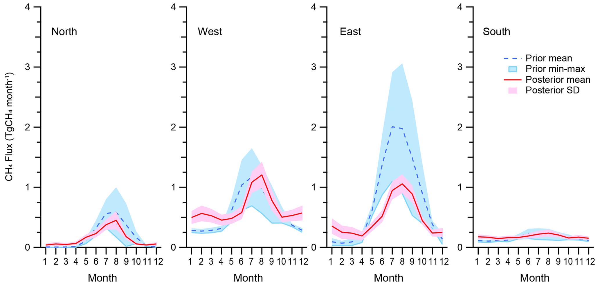
Figure 9Seasonal cycles of CH4 fluxes for subregions (North, West, East, and South). Solid red lines and red shaded areas indicate the mean posterior monthly emissions and standard deviations (SD) from 24 experiments in Inv_4R12S for 2012–2017. Dotted blue lines and blue shaded areas indicate mean prior emissions and their minima and maxima.
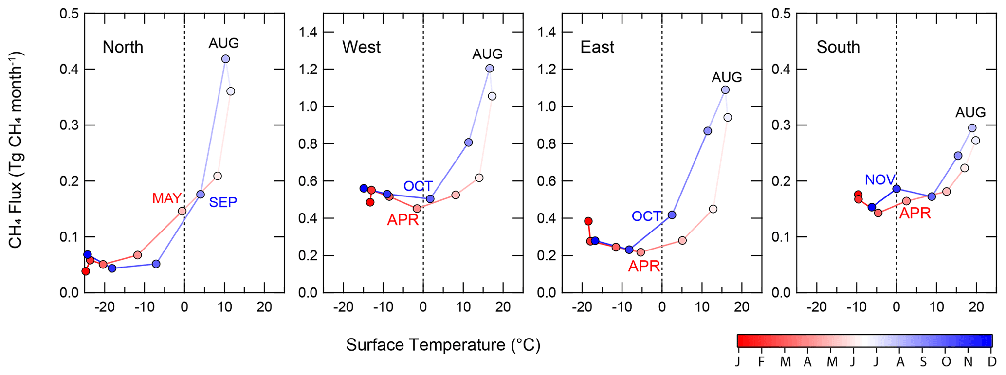
Figure 10Dependency of mean posterior monthly CH4 fluxes on monthly mean air surface temperature. The inversion results and the air temperature data at 2 m above the ground from NCEP reanalysis are averaged for 2012–2017 and aggregated over the subregions.
3.4.1 Seasonal cycle
Figure 9 shows the ensemble mean comparison of the seasonal cycles between the posterior fluxes and the prior fluxes from 2012 to 2017 for each subregion. The prior fluxes in the subregions with significant wetland emissions (North, East, and West) show strong maxima in the summer when wetland emissions are most active. The four different wetland priors have very different maxima, giving the large ranges of summer fluxes in Fig. 9. The posterior fluxes from inversions are much reduced in the summer, particularly in the subregion East containing the HBL. Differences in seasonal phase between the prior and posterior are evident in East and West. The spring increase in CH4 emissions is delayed by about 2 months in the posterior fluxes compared to the prior fluxes, and the summer maxima appear late by 1 month from June–July to July–August. In September, the posterior fluxes remain high compared to the priors. This seasonal phase shift in posterior fluxes suggests that surface air temperature is not the sole driver of the seasonality of wetland CH4 fluxes. Temperature has been widely found to be a major driver to constrain the seasonal cycle of wetland CH4 emissions, but their relationship might not be linear. Other factors, such as carbon substrates and seasonal inundation, are also drivers of wetland CH4 seasonality (Delwiche et al., 2021). This result is consistent with the hysteretic temperature sensitivity of wetland CH4 fluxes demonstrated by Chang et al. (2020), yielding more CH4 emissions later in the warm season. Instead of a single temperature dependency in wetland model parameterizations, Chang et al. (2020) proposed the microbial-substrate-mediated CH4 production hysteresis; higher substrate (i.e., acetate and hydrogen) availability during the later period stimulates higher methanogen biomass. While Chang et al. (2020) validated their wetland model results with chamber field measurements, the present study examined the temperature dependency on a subregional scale using our mean posterior fluxes and surface air temperature at 2 m above ground from NCEP reanalysis (Kalnay et al., 1996). As seen in Fig. 10, the posterior fluxes, especially in East and West, show that surface air temperature dependency varies between the early and the later periods in the warm season (air temperature > 0 °C), supporting the hysteretic temperature sensitivity hypothesis on the regional scale. The consistency between our results and Chang et al. (2020) supports the hypothesis that the wetland CH4 emissions drive the seasonality of our posterior fluxes.
In contrast to the reduced posterior summer fluxes, the posterior fluxes are higher during the cold winter season than the prior fluxes in both East and West. The presence of higher fluxes in East with little anthropogenic fluxes suggests the wetland emission in the winter is higher than the ecosystem model results used as priors. Also, our winter flux results are not consistent with the previous regional inversion results (e.g., Miller et al., 2014; Thompson et al., 2017), which do not show any large winter fraction (∼ 10 %) of CH4 emissions in the HBL compared to our results for East (22 %; see Sect. 3.5.2). The potential natural/wetland CH4 emissions in the cold season are discussed in Sect. 3.6. As seen in Figs. 9 and S10, the range of variation in fluxes for the prior is different from the posterior. As the dominant fluxes are from wetlands in the summer, the wide range of prior fluxes reflects the uncertainties in the different wetland process models, including wetland types and spatial distributions and functional dependence on climate forcing. Using the atmospheric CH4 to constrain the summer emissions yielded posterior variations smaller than the priors. The inversion of the spatially distributed wetland fluxes (as seen in Fig. 3a and c) appears less sensitive to errors/differences among our transport models or prior flux magnitudes, giving smaller variations or more robust flux estimates in the summer posterior fluxes. In contrast, with locally non-homogeneous anthropogenic fluxes (Fig. 3b and d), transport errors appear more important in the winter, resulting in larger variability in the posterior fluxes than the prior fluxes. The anthropogenic fluxes are predominantly distributed in western Canada; the posterior fluxes in West exhibit large transport dependency in the winter (Fig. S10).
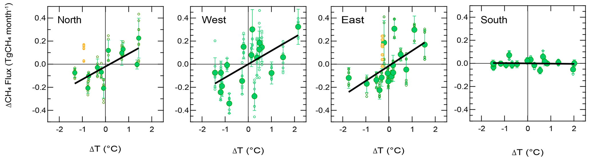
Figure 11Flux–temperature relationship in the summer season. Fluxes are the anomalies of estimated monthly fluxes from the 6-year (2012–2017) monthly mean fluxes. Temperature is the regional monthly anomaly from the same 6-year (2012–2017) monthly mean temperature. The summer season is defined as July and August for North and July to September for the remaining subregions. Closed green circles are the ensemble mean flux anomalies, error bars denote the standard deviation (SD), and open green circles are the anomalies of 24 individual experiments. The yellow circles are from the estimated fluxes, which are excluded because the nearby forest fires apparently affected the flux estimates.
3.4.2 Inter-annual variation and relationship with climate anomalies
As presented in Sect. 3.2, the inter-annual variations in the subregions among the inversions are comparable to or greater than the respective long-term trends. To examine the drivers of inter-annual variability in CH4 fluxes, we focus on the later period from 2012 to 2017, when the inversions are constrained with better observation coverage. The inter-annual variability in the later period tends to be smaller than in the early period (Fig. 7). This tendency may be related to the number of observational constraints on the inversions. The year-to-year change in posterior annual fluxes for Canada is relatively small: standard deviation (SD) of 0.6 Tg CH4 yr−1 is ∼ 3 % of the mean flux of 17.4 Tg CH4 yr−1 (Fig. 7). In all the regions except for North, the SD of the posterior annual fluxes is < ∼ 8 %, while North shows an SD of ∼ 18 % of the posterior annual fluxes (Fig. S6). The correlations of the posterior fluxes among the subregions and between the subregions and the nation are summarized in Table S3. Overall, no clear relationship among the subregional emission changes is found. There are no significant correlations of the year-to-year change in the posterior fluxes among the subregions, r = −0.38 to 0.37 (p > 0.43), except for the correlation between East and South (r = 0.82, p = 0.05). The subregional flux changes are not correlated with the national flux, r = −0.12 to 0.40 (p > 0.42), while only North shows an apparent correlation (r = 0.74, p = 0.09). Given the large geographical size of Canada, the low correlations of the posterior fluxes among the subregions indicate that the drivers of inter-annual variations in CH4 flux may be subregional-scale processes, such as synoptic systems (of temperature and precipitation variations) with a weekly timescale and ∼ 1000 km spatial scale. Furthermore, on a subregional scale, the summer flux changes appear to drive the inter-annual variations in subregional fluxes. The year-to-year change in the annual flux for each subregion is well correlated with the summertime (July and August for North, July to September for the other subregions) flux anomaly within the respective subregions: r = 0.97 (North), 0.71 (West), 0.90 (East), and 0.77 (South). The high correlations suggest that the change in natural summer CH4 emission is a major factor in the inter-annual variability in Canada's CH4 fluxes.
Thus, we examined the statistical correlation between flux anomalies and temperature anomalies by subregion for the period of 2012 to 2017. For this, surface air temperature anomalies from NCEP reanalysis (Kalnay et al., 1996) are aggregated to the respective subregions. The correlations between the monthly flux anomalies and monthly surface air temperature anomalies for the summer months are shown in Fig. 11. The inter-annual variability in posterior CH4 fluxes for subregions North, West, and East exhibits moderate positive correlation with the surface temperature anomaly: r = 0.64 (p < 0.01, North), r = 0.60 (p = 0.01, West), r = 0.60 (p = 0.01, East), but r = −0.06 (p = 0.81, South), as visualized in Fig. 11.
In South, no robust correlation is found between the posterior fluxes and climate on seasonal and monthly scales (Fig. 11). This is consistent with the prior fluxes in the subregion South being mainly (annually constant) anthropogenic fluxes and a small component of natural wetland fluxes. It also serves as a check on the annually constant assumption for the anthropogenic fluxes. The relatively strong flux–temperature dependence in three of the four subregions (Fig. 11) suggests that wetland CH4 emission could be enhanced with climate change and warming.
The correlation of inter-annual variability in posterior CH4 fluxes with the surface temperature anomaly is evident on shorter monthly timescales also. The correlations by month are shown in Table S4 and Fig. S11. Overall, the posterior fluxes and temperature anomalies show positive correlations. The wildfire component of the posterior flux, which is not necessarily correlated to temperature, might affect the correlations between the posterior fluxes and temperature anomalies. According to a fire monitoring system (Canadian Wildland Fire Information System, https://cwfis.cfs.nrcan.gc.ca, last access: 10 October 2023), severe wildfires started at the end of June 2014 around BCK in North and continued until early August, causing a higher level of CH4 biomass burning emissions. Near FSD in East, in August 2017, local wildfire events in northwestern Ontario apparently caused high CH4 emissions. If these possibly wildfire-induced positive CH4 emission anomalies are removed, the positive correlations with air temperature anomalies in North and East are improved, as monthly correlations are enhanced by ∼ 50 % (Table S4 and Fig. S11). Due to the short summer in North, clear correlations are found only for July and August. In West and East, the posterior fluxes in early summer, June, are less sensitive to air temperature anomalies than in the following summer months, including September. This high-sensitivity summer period is consistent with the active natural summer emission period, as discussed in Sect. 3.4.1.
For comparison, the same analysis was done for the different prior fluxes with inter-annual variations (WetCHARTs, CLASSICdiag, CLASSICprog) used in this study, and the results are shown in Fig. S12. Only CLASSICdiag in East shows a positive temperature dependence (r = 0.52, similar to the inversion results in Fig. 11), and the slope of the linear fit or flux–temperature sensitivity in CLASSICdiag is about half as large compared to the posterior flux. The other subregions and other prior fluxes show no clear dependence on temperature. These results suggest that many factors govern the wetland CH4 fluxes. For example, there are large differences in the spatial distribution for the different priors (see Fig. 3a). More studies are needed to understand the flux–climate relationship better.
We also examined the correlation between flux anomalies with the precipitation anomalies with no lag to a 2-month lag, but no significant correlation was found (|r| < 0.2, p > 0.3).
3.5 National and regional distribution of annual fluxes
3.5.1 Total CH4 emissions
Figure 12 shows the total (natural and anthropogenic) annual mean CH4 emission estimates for Canada compared with prior fluxes and previous inversion studies. Our mean posterior flux for Canada is 17.4 (15.3–19.5) Tg CH4 yr−1 and is near the lower end of the range of prior fluxes but quite similar to the prior flux scenarios with CLASSIC prognostic wetland CH4 fluxes (CLASSICprog_ECAQ and CLASSICprog_EDGAR). Compared with global inversion studies, our estimate is slightly lower (by ∼ 1.5 Tg CH4 yr−1) than the GCP-CH4 global inversion ensemble mean but within uncertainties. However, the CarbonTracker-CH4 value of 10.2 Tg CH4 yr−1 (Bruhwiler et al., 2014) is substantially lower than our estimate. The regional inversions by Miller et al. (2014) and Thompson et al. (2017) do not cover the entirety of Canada but partially cover the regions south of 65° N and north of 50° N, respectively. Therefore, these differences should be noted in the comparison with these two previous regional inversions. The national flux estimate by Miller et al. (2014), 21.3 ± 1.6 Tg CH4 yr−1, is more than double that of their priors (7.6–9.4Tg CH4 yr−1). Miller et al. (2014) explained that the higher flux estimates might be attributed to the anthropogenic emissions in the province of Alberta in western Canada. Thompson et al. (2017) also estimated the larger anthropogenic emissions in Alberta, 4.3 ± 1.3 Tg CH4 yr−1, nearly 3 times higher than their prior emission based on EDGAR-4.2FT2010 (Janssens-Maenhout et al., 2014). However, their estimated national total emission is slightly lower than our estimates, possibly because of their model domain. Thompson et al. (2017) did not include southern Ontario and Quebec, the densely populated area in Canada.

Figure 12Estimated mean total CH4 emissions for Canada for 2012–2017 (solid purple bar). The mean of the eight prior flux scenarios is shown in the unshaded purple bar, along with each mean of individual prior scenarios. For comparison, the previous global and regional inversion results are plotted in gray and light green bars, respectively. Global: GELCA (2012–2017), CT-CH4 (2000–2010), and GCP-CH4 inversion ensemble (2008–2017). Regional: Miller et al. (2014) cover up to 65° N for 2007–2008, while Thompson et al. (2017) cover north of 50° N for 2005–2013.
Some spatial differences can be seen in this study compared to the priors and global inverse models. At the subregional level, the mean prior flux distribution shows larger emissions in East than West (the spatial distributions of the prior scenarios are shown in Fig. S13). Similarly, global inversions (CT-CH4 and GELCA-CH4) show larger emission in East than West. Only this study shows higher CH4 emission in West than in East within Canada (Fig. S13). For the subregion North, the Canadian Arctic, there are considerable differences among the priors: 1.4 to 4.2 Tg CH4 yr−1. The CH4 emission estimated in this study is 1.8 ± 0.6 Tg CH4 yr−1, consistent with our previous study, 1.8 ± 0.6 Tg CH4 yr−1 (Ishizawa et al., 2019, for the years 2012 to 2015).
3.5.2 Natural and anthropogenic CH4 sources
As a first attempt of total emission breakdown into natural and anthropogenic sources with the scheme presented in Sect. 2.3, we assumed Rcold (fraction of cold season's natural CH4 emission to its annual emission) to be in the range of 0 % to 10 % based on wetland models and previous studies (see Sect. 2.3 and Fig. 3e). Then, the anthropogenic emissions are approximately 12 Tg CH4 yr−1 for Canada, 6.3 Tg CH4 yr−1 for West, and 2.8 Tg CH4 yr−1 for East. These anthropogenic CH4 emission values are much larger than the priors: more than twice as large as those for Canada and West from the prior inventories and more than 6 times those of the priors (∼ 0.45 Tg CH4 yr−1) for East. These resultant national and subregional anthropogenic emissions seem excessive when compared to the several regional inversion studies with larger estimates of anthropogenic fluxes than the inventories, especially in West (e.g., Miller et al., 2014; Thompson et al., 2017; Chan et al., 2020; Baray et al., 2021). Even if there is potential for higher anthropogenic emission in West, the estimated anthropogenic emission in East seems unrealistic, where there is no significant anthropogenic CH4 emitter according to the priors.
Next, we explored an alternative approach assuming that the natural CH4 production is more active in the cold season than as predicted by the prior wetland models. Such a cold-season wetland CH4 emission has been reported by previous observation-based studies (e.g., Pelletier et al., 2007; Zona et al., 2016). Zona et al. (2016) explained CH4 emissions in the Arctic tundra continue even in the cold season due to the “zero curtain”. When air temperatures drop to around 0 °C, there is a period when the water trapped in the soil below the surface has not frozen completely. Micro-organisms in the unfrozen layer remain active and emit CH4 into the atmosphere. CH4 emission in cold months, September to May, could account for ≥ 50 % of annual CH4 emission in the Arctic.
As seen in Sect. 3.4.1, the posterior CH4 fluxes in this study show notable winter emissions, which could be potential winter (or cold season) natural/wetland fluxes in subregions with little anthropogenic CH4, such as East and North (Figs. 9 and 10). Thus, we derived the winter natural flux fractions Rcold from our estimated mean seasonal CH4 fluxes by assuming that the (seasonally non-varying) anthropogenic fluxes are the mean prior anthropogenic fluxes of 0.45 Tg CH4 yr−1 for November to March in East and 0.01 Tg CH4 yr−1 for October to May in North (the uncertainties in these prior fluxes are examined below). Then, solving Eqs. (6) and (7), Rcold is 22 (20–24) % for East and 30 (29–32) % for North. We applied the Rcold derived for the subregion East to the subregions West and South, as these subregions are also located in the mid-latitudes with similar temperature and growing conditions.
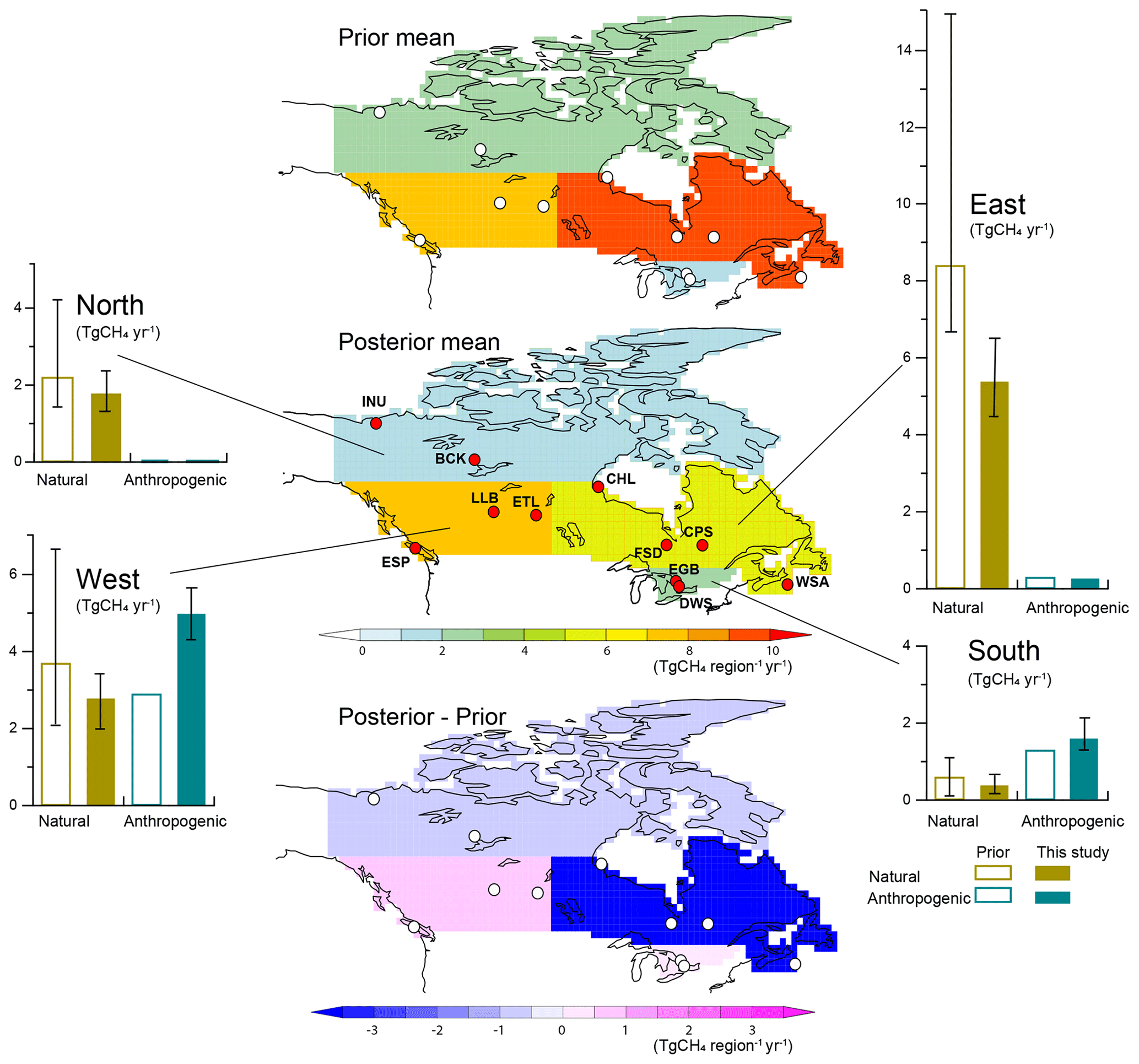
Figure 13Mean spatial distribution of prior total flux (top), posterior total flux (middle), and the difference between posterior and prior (bottom). Posterior emissions partitioned into natural and anthropogenic sources by subregion, along with the respective prior-emission means and ranges (min–max), are shown on the left and right sides.
The resultant mean natural and anthropogenic CH4 fluxes for the subregions are shown in Fig. 13, along with the mean prior fluxes. For Canada, our estimate for natural emissions, 10.8 (7.5–13.2) Tg CH4 yr−1, is smaller than most of the process-based ecosystem model estimates, while our anthropogenic emission estimate, 6.6 (6.2–7.8) Tg CH4 yr−1, is larger than the inventories, 3.5 to 5.2 Tg CH4 yr−1 (Ito, 2021; Stavert et al., 2021), primarily attributed to western Canada. The anthropogenic emission in this study for West, 5.0 (4.6–5.6) Tg CH4 yr−1, is comparable with previous regional anthropogenic emission estimates (e.g., Miller et al., 2014; Thompson et al., 2017; Baray et al., 2021; Fujita et al., 2018). Chan et al. (2020) estimated nearly twice the amount of CH4 emissions from the oil and gas sector in Alberta and the adjacent province of Saskatchewan than the NIR (higher by 1.6 Tg CH4 yr−1), based on the 8-year wintertime atmospheric surface measurements. Baray et al. (2021) also attributed their estimated national anthropogenic CH4 emissions (6.0–6.5 Tg CH4 yr−1), higher than the NIR, to western Canada (4.7 ± 0.6 Tg CH4 yr−1, for the provinces of British Columbia, Alberta, Saskatchewan, and Manitoba), using ECCC surface measurements and Greenhouse Gases Observing Satellite (GOSAT) data to constrain their inverse model. Fujita et al. (2018) inferred that an additional time-invariant (anthropogenic) emission of 2.6 ± 0.3 Tg CH4 yr−1 is required in the EDGAR inventory in Alberta to make their model simulation closer to the observed CH4 mixing ratios at Churchill.
One assumption in the flux partition analysis is that the posterior anthropogenic fluxes for the subregions North and East are the same as their priors in Eqs. (6) and (7). The sensitivity of the flux partitioning to this assumption was examined by repeating the analysis with halving and doubling their values. The results for the estimated anthropogenic CH4 fluxes for Canada and the subregions West and South changed by < 5 %. Thus, the flux partitioning appears stable and capable of detecting the higher anthropogenic CH4 flux from West.
3.6 Winter natural CH4 emissions
Results for cold-season natural CH4 fluxes are wide-ranging among recent studies, as cold-season natural CH4 fluxes are difficult to measure and quite variable in wetland model estimates. Treat et al. (2018) reported a measured cold-season (non-growing) fraction of wetland CH4 of 16 % (95 % confidence interval, CI, 11.0 %–23.0 %) between 40 and 60° N and 17 % (CI 16.0 %–23.3 %) for north of 60° N. These fractions tend to be higher than process-based models (4 %–17 % within 40–60° N), while the upscaled flux estimates based on the flux measurement with machine learning technique (Peltola et al., 2019) showed cold-season (November to March) emissions of ∼ 20 % for north of 45° N. Pelletier et al. (2007) reported up to 13 % of the annual emission in the winter (November to March), in peatland in James Bay Lowland, along the Hudson Bay coastline in Canada. A recently published CH4 flux dataset from the flux measurement global network (FLUXNET-CH4) has a considerable contribution of cold months (October to March) to annual CH4 flux of 18.1 ± 3.6 % and 15.3 ± 0.1 % in northern (> 60° N) and temperate (40–60° N) regions, respectively (Delwiche et al., 2021). An inter-comparison of 16 wetland models from the Global Carbon Project (Ito et al., 2023) showed cold-season CH4 fluxes (September to May) ranging from 11.6 %–40.1 % in the Arctic (> 60° N) and 21.6 %–54 % north of 45° N. For comparison, our cold-season (September to May) natural CH4 emissions are 38.5 (38–39) % in the Arctic (> 60° N) and 51 (49–52) % north of 45° N. The natural CH4 emission in this study is not directly comparable to the other wetland emissions as our natural CH4 emission is limited to the model domain of Canada and includes biomass burning and soil sink. But our natural CH4 emission estimate appears to be within the range of results of other studies. As the range of possible winter wetland emission fractions is large in previous studies, evidence of winter wetland and natural CH4 emissions in our atmospheric CH4 measurements is further examined in the following section.
3.6.1 Signals of winter natural CH4 emissions in observations
The partition of total CH4 flux into anthropogenic and natural components in Sect. 3.5.2 indicates the presence of natural emissions in the winter or cold (non-growing) season. In this section, we examine the observed atmospheric CH4 to determine if it is possible to see the signature of winter CH4 emissions from the natural component. Emissions near an observation site have a measurable temporal signal in the atmospheric CH4. The atmospheric CH4 is temporally modulated by the interaction of the diurnal cycle in the planetary boundary layer (PBL) with the nearby emissions, resulting in a diurnal cycle in the observed atmospheric CH4 with a higher mixing ratio during nighttime (during shallow PBL) and a lower mixing ratio during daytime (during a well-mixed deep PBL). This is the diurnal rectifier effect (Denning et al., 1996) for constant or slow-changing emissions. Other factors like strong winds and cloudiness can affect the diurnal interaction. However, the coupling of PBL dynamics with local emissions should be evident statistically in the monthly average diurnal cycle of the mixing ratios with sufficiently large emissions (discussed below). Although the diurnal cycle of the mixing ratio is a qualitative indicator of local emissions, it could be viewed as a consistency evaluation of the inversion result.
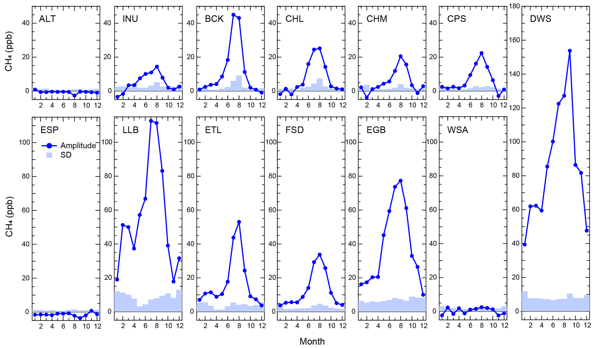
Figure 14Seasonal cycles of normalized diurnal amplitude and standard deviation (SD) of observed atmospheric CH4 during the afternoon mean (14:00–16:00 LT, the reference of normalization).
The monthly mean diurnal amplitude at each measurement site was obtained as follows. Firstly, we calculated a normalized diurnal cycle, defining the mean afternoon mixing ratio over the local times between 14:00 and 16:00 LT as a reference. Secondly, the individual normalized diurnal cycles were averaged by month over the measurement periods (Fig. S14). Then, we obtained the monthly mean diurnal amplitude as a maximum mixing ratio difference from the respective reference afternoon mixing ratio during 24 h (00:00 to 24:00 UTC). The results are shown in Fig. 14, along with the monthly standard deviations (SDs) of the afternoon atmospheric CH4, which is a measure of the variability in the (reference) afternoon mixing ratio. When the monthly diurnal cycle of atmospheric CH4 is larger than the monthly afternoon mixing ratio SD (a detectable signal above the expected variability), this is used as an indirect indication of the presence of CH4 fluxes around the measurement site.
For the baseline (coastal) sites ALT, ESP, and WSA with negligible CH4 fluxes nearby (Fig. 14), the diurnal cycles in atmospheric CH4 are absent as expected. For the urban site DWS located in the city of Toronto, with anthropogenic CH4 fluxes throughout the year, the diurnal cycle is much larger than the SD in both winter (59 ppb, averaging from November to March) and summer (105 ppb, averaging from April to October). The summer diurnal cycle is much stronger than the winter as the PBL has the strongest day–night contrast with strong solar heating during daytime and radiative cooling at nighttime. The diurnal cycle for the near-urban site EGB, ∼ 100 km away from Toronto, is about 50 % as large as DWS with the strong anthropogenic emission. Thus, the diurnal cycle of atmospheric CH4 is sensitive to the emissions from an approximately 100 km radius area.
For the remaining arctic and boreal forest sites (INU, BCK, CHL, CHM, CPS, LLB, ETL, FSD), the strong summer diurnal cycles of mixing ratios are clearly exhibited with amplitudes of ∼ 15 to 110 ppb (Fig. 14). Since these boreal forest sites are far from anthropogenic sources, the strong diurnal cycles in summer are indications of natural summer CH4 sources near the sites. In the winter, there are clear diurnal cycles at LLB, ETL, and FSD (5 to 20 ppb and clearly higher than the respective afternoon SD). These sites are located near strong wetland sources according to the map of prior fluxes shown in Fig. 3a. The indication of winter natural emissions in the observed diurnal cycle in mixing ratios is consistent with the inversion results discussed in Sect. 3.5.2. The weaker winter diurnal cycles at INU, BCK, CHL, CHM, and CPS suggest weaker natural emissions, which is consistent with their locations of weaker prior fluxes (see Fig. 3a). Another factor for the weaker winter diurnal cycles in the high latitudes or arctic region observation sites is the weak winter solar forcing and the correspondingly shallow PBL diurnal cycles. Some caveats relating to the diurnal cycle of the mixing ratio at observation sites and inversion flux results are that the area of influence for diurnal cycles in mixing ratios is much smaller than the inversion subregions. Thus, though comparing an indirect feature of emissions (diurnal amplitude) to the quantitative inverse flux estimates requires caution, overall, the diurnal cycles in observed mixing ratios appear consistent with the inversion results.
In this study, we estimated the CH4 fluxes in Canada using an inverse model constrained with ECCC's network of continuous surface atmospheric CH4 measurements. The Bayesian inverse model included an ensemble of prior fluxes and atmospheric transport models to estimate the posterior flux uncertainties associated with these model variations. We analyzed the variability or robustness of the posterior flux estimates as a function of model resolution (number of subregions), quantity of observations (number of observation sites), and the spatiotemporal relationship of the posterior fluxes to climatological forcing.
Sensitivity experiments comparing different subregion masks (up to six subregions) were done to examine the variability in the posterior flux estimates. Results indicate that, with the set of 12 observation sites, the inverse model yields more stable and physical results (with no unphysical negative fluxes) for the 4-subregion mask setting (the reference inversion). The earlier period (2007–2011) with fewer measurement sites (without BCK or INU) has more variability in the flux estimates and unphysical negative posterior fluxes, primarily in western Canada.
The reference inversion experiment ensemble mean estimate of total CH4 flux for Canada (2012–2017) is 17.4 (15.3–19.5) Tg CH4 yr−1. This total is partitioned into 10.8 (7.5–13.2) Tg CH4 yr−1 of natural sources and 6.6 (6.2–7.8) Tg CH4 yr−1 of anthropogenic sources. In this study, the natural CH4 source is still the major CH4 emitter in Canada, especially in eastern Canada, though our estimated natural emissions are lower than most previous bottom-up estimates. By contrast, the anthropogenic CH4 source estimates are higher than the inventory estimates, primarily in western Canada. The higher anthropogenic emission in western Canada is consistent with previous regional anthropogenic top-down emission estimates (e.g., Chan et al., 2020).
The reference inversion results for 2012–2017 were analyzed for other physical characteristics including the temporal, spatial, and statistical properties as well as a possible relationship to climatological forcing. Compared to other inversion studies, some notable results in our flux estimates include a quantifiable amount of winter wetland CH4 emissions (November–March with 20 %–24 % of the annual emissions for boreal regions and October–May with 29 %–32 % for subarctic region), hysteretic temperature dependence for wetland emissions over the warm (growing) season, and apparent correlation of wetland summer fluxes with mean summer temperature anomalies in Canada. No significant trend is found in the estimated decadal CH4 emissions (the trend is within the flux estimate uncertainties), in contrast to some studies reporting long-term trends. The differences from other inversion studies could be related to having more in situ measurement sites and focusing the inversion domain on Canada. This study also showed that the spatial mixing ratio gradients among the sites could be an independent verification tool of the posterior fluxes.
The measurement network across the nation is essential to improve our ability not only to quantify how Canada's natural CH4 emissions will respond to climate change, but also to monitor anthropogenic CH4 emission trends in response to Canada's CH4 reduction efforts. These regional inversion results, which reflect better observational constraints on the regional scale of space and seasonal timescale, might help wetland process models to improve their sensitivity to and functions for climate parameters. Improvements in wetland process models and anthropogenic emissions could lead to improving regional climate model predictions.
The ECCC observations are available from the World Data Centre for Greenhouse Gases (WDCGG) at https://gaw.kishou.go.jp/ (WDCGG, 2023) and the NOAA Observation Package (ObsPack) at https://doi.org/10.25925/20231201 (Schuldt et al., 2023).
The supplement related to this article is available online at: https://doi.org/10.5194/acp-24-10013-2024-supplement.
MI and DC designed the research. MI conducted all inversions and data analysis, wrote the initial draft, and edited it together with DC. DW led the ECCC GHG measurement program. MI, DC, and EC provided and processed footprint data for the inversion. JRM and VKA provided the CLASSIC wetland CH4 fluxes. All co-authors reviewed the manuscript and contributed to the discussion and revision.
The contact author has declared that none of the authors has any competing interests.
Publisher's note: Copernicus Publications remains neutral with regard to jurisdictional claims made in the text, published maps, institutional affiliations, or any other geographical representation in this paper. While Copernicus Publications makes every effort to include appropriate place names, the final responsibility lies with the authors.
We are grateful to the NOAA CarbonTracker-Lagrange (CT-L) program for providing the WRF-STILT footprint data of Canadian sites for our inversion study. We acknowledge the Global Carbon Project CH4 modelling group (Saunois et al., 2020) for the prior wetland CH4 emission data used in this study and the posterior national emission estimates for Canada, as well as Lori Bruhwiler for providing CarbonTracker-CH4 results and Rona Thompson for providing FLEXINVERT CH4 inversion results for the analysis in this study. We thank the team members of ECCC's Greenhouse Gases Measurement Laboratory, Larry Giroux, Bob Kessler, and Senen Racki, for collecting the observations and maintaining the ECCC GHG measurement network.
This paper was edited by Robert McLaren and reviewed by two anonymous referees.
Baray, S., Darlington, A., Gordon, M., Hayden, K. L., Leithead, A., Li, S.-M., Liu, P. S. K., Mittermeier, R. L., Moussa, S. G., O'Brien, J., Staebler, R., Wolde, M., Worthy, D., and McLaren, R.: Quantification of methane sources in the Athabasca Oil Sands Region of Alberta by aircraft mass balance, Atmos. Chem. Phys., 18, 7361–7378, https://doi.org/10.5194/acp-18-7361-2018, 2018.
Baray, S., Jacob, D. J., Maasakkers, J. D., Sheng, J.-X., Sulprizio, M. P., Jones, D. B. A., Bloom, A. A., and McLaren, R.: Estimating 2010–2015 anthropogenic and natural methane emissions in Canada using ECCC surface and GOSAT satellite observations, Atmos. Chem. Phys., 21, 18101–18121, https://doi.org/10.5194/acp-21-18101-2021, 2021.
Bloom, A. A., Bowman, K. W., Lee, M., Turner, A. J., Schroeder, R., Worden, J. R., Weidner, R., McDonald, K. C., and Jacob, D. J.: A global wetland methane emissions and uncertainty dataset for atmospheric chemical transport models (WetCHARTs version 1.0), Geosci. Model Dev., 10, 2141–2156, https://doi.org/10.5194/gmd-10-2141-2017, 2017.
Bréon, F. M., Broquet, G., Puygrenier, V., Chevallier, F., Xueref-Remy, I., Ramonet, M., Dieudonné, E., Lopez, M., Schmidt, M., Perrussel, O., and Ciais, P.: An attempt at estimating Paris area CO2 emissions from atmospheric concentration measurements, Atmos. Chem. Phys., 15, 1707–1724, https://doi.org/10.5194/acp-15-1707-2015, 2015.
Bruhwiler, L., Dlugokencky, E., Masarie, K., Ishizawa, M., Andrews, A., Miller, J., Sweeney, C., Tans, P., and Worthy, D.: CarbonTracker-CH4: an assimilation system for estimating emissions of atmospheric methane, Atmos. Chem. Phys., 14, 8269–8293, https://doi.org/10.5194/acp-14-8269-2014, 2014.
CCAC: Global Methane Pledge, https://www.globalmethanepledge.org/ (last access: 6 September 2023), 2023.
Chan, E., Worthy, D. E. J., Chan, D., Ishizawa, M., Moran, M. D., Delcloo, A., and Vogel, F.: Eight-Year Estimates of Methane Emissions from Oil and Gas Operations in Western Canada Are Nearly Twice Those Reported in Inventories, Environ. Sci. Technol., 54, 14899–14909, https://doi.org/10.1021/acs.est.0c04117, 2020.
Chang, K.-Y., Riley, W. J., Crill, P. M., Grant, R. F., and Saleska, S. R.: Hysteretic temperature sensitivity of wetland CH4 fluxes explained by substrate availability and microbial activity, Biogeosciences, 17, 5849–5860, https://doi.org/10.5194/bg-17-5849-2020, 2020.
Cooper, O. R., Parrish, D. D., Stohl, A., Trainer, M., Nédélec, P., Thouret, V., Cammas, J. P., Oltmans, S. J., Johnson, B. J., Tarasick, D., Leblanc, T., McDermid, I. S., Jaffe, D., Gao, R., Stith, J., Ryerson, T., Aikin, K., Campos, T., Weinheimer, A., and Avery, M. A.: Increasing springtime ozone mixing ratios in the free troposphere over western North America, Nature, 463, 344–348, https://doi.org/10.1038/nature08708, 2010.
Dee, D. P., Uppala, S. M., Simmons, A. J., Berrisford, P., Poli, P., Kobayashi, S., Andrae, U., Balmaseda, M. A., Balsamo, G., Bauer, P., Bechtold, P., Beljaars, A. C. M., van de Berg, L., Bidlot, J., Bormann, N., Delsol, C., Dragani, R., Fuentes, M., Geer, A. J., Haimberger, L., Healy, S. B., Hersbach, H., Hólm, E. V., Isaksen, L., Kållberg, P., Köhler, M., Matricardi, M., McNally, A. P., Monge-Sanz, B. M., Morcrette, J. J., Park, B. K., Peubey, C., de Rosnay, P., Tavolato, C., Thépaut, J. N., and Vitart, F.: The ERA-Interim reanalysis: configuration and performance of the data assimilation system, Q. J. Roy. Meteor. Soc., 137, 553–597, https://doi.org/10.1002/qj.828, 2011.
Delwiche, K. B., Knox, S. H., Malhotra, A., Fluet-Chouinard, E., McNicol, G., Feron, S., Ouyang, Z., Papale, D., Trotta, C., Canfora, E., Cheah, Y.-W., Christianson, D., Alberto, Ma. C. R., Alekseychik, P., Aurela, M., Baldocchi, D., Bansal, S., Billesbach, D. P., Bohrer, G., Bracho, R., Buchmann, N., Campbell, D. I., Celis, G., Chen, J., Chen, W., Chu, H., Dalmagro, H. J., Dengel, S., Desai, A. R., Detto, M., Dolman, H., Eichelmann, E., Euskirchen, E., Famulari, D., Fuchs, K., Goeckede, M., Gogo, S., Gondwe, M. J., Goodrich, J. P., Gottschalk, P., Graham, S. L., Heimann, M., Helbig, M., Helfter, C., Hemes, K. S., Hirano, T., Hollinger, D., Hörtnagl, L., Iwata, H., Jacotot, A., Jurasinski, G., Kang, M., Kasak, K., King, J., Klatt, J., Koebsch, F., Krauss, K. W., Lai, D. Y. F., Lohila, A., Mammarella, I., Belelli Marchesini, L., Manca, G., Matthes, J. H., Maximov, T., Merbold, L., Mitra, B., Morin, T. H., Nemitz, E., Nilsson, M. B., Niu, S., Oechel, W. C., Oikawa, P. Y., Ono, K., Peichl, M., Peltola, O., Reba, M. L., Richardson, A. D., Riley, W., Runkle, B. R. K., Ryu, Y., Sachs, T., Sakabe, A., Sanchez, C. R., Schuur, E. A., Schäfer, K. V. R., Sonnentag, O., Sparks, J. P., Stuart-Haëntjens, E., Sturtevant, C., Sullivan, R. C., Szutu, D. J., Thom, J. E., Torn, M. S., Tuittila, E.-S., Turner, J., Ueyama, M., Valach, A. C., Vargas, R., Varlagin, A., Vazquez-Lule, A., Verfaillie, J. G., Vesala, T., Vourlitis, G. L., Ward, E. J., Wille, C., Wohlfahrt, G., Wong, G. X., Zhang, Z., Zona, D., Windham-Myers, L., Poulter, B., and Jackson, R. B.: FLUXNET-CH4: a global, multi-ecosystem dataset and analysis of methane seasonality from freshwater wetlands, Earth Syst. Sci. Data, 13, 3607–3689, https://doi.org/10.5194/essd-13-3607-2021, 2021.
Denning, A. S., Collatz, G. J., Zhang, C., Randall, D. A., Berry, J. A., Sellers, P. J., Colello, G. D., and Dazlich, D. A.: Simulations of terrestrial carbon metabolism and atmospheric CO2 in a general circulation model, Tellus B, 48, 521–542, https://doi.org/10.3402/tellusb.v48i4.15930, 1996.
Dirmeyer, P. A., Gao, X., Zhao, M., Guo, Z., Oki, T., and Hanasaki, N.: GSWP-2: Multimodel Analysis and Implications for Our Perception of the Land Surface, B. Am. Meteorol. Soc., 87, 1381–1398, https://doi.org/10.1175/BAMS-87-10-1381, 2006.
Dlugokencky, E. J., Myers, R. C., Lang, P. M., Masarie, K. A., Crotwell, A. M., Thoning, K. W., Hall, B. D., Elkins, J. W., and Steele, L. P.: Conversion of NOAA atmospheric dry air CH4 mole fractions to a gravimetrically prepared standard scale, J. Geophys. Res., 110, D18306, https://doi.org/10.1029/2005jd006035, 2005.
ECCC: Canadian Environmental Sustainability Indicators: Extent of Canada's Wetlands, https://www.canada.ca/en/environment-climate-change/services/environmental-indicators/extent-wetlands.html (last access: 24 May 2024), 2016.
ECCC: National Inventory Report 1990–2020: Greenhouse gas sources and sinks in Canada, Part 3, https://publications.gc.ca/collections/collection_2022/eccc/En81-4-2020-3-eng.pdf (last access: 10 October 2023), 2022.
Fan, S., Gloor, M., Mahlman, J., Pacala, S., Sarmiento, J., Takahashi, T., and Tans, P.: A Large Terrestrial Carbon Sink in North America Implied by Atmospheric and Oceanic Carbon Dioxide Data and Models, Science, 282, 442–446, https://doi.org/10.1126/science.282.5388.442, 1998.
Fujita, R., Morimoto, S., Umezawa, T., Ishijima, K., Patra, P. K., Worthy, D. E. J., Goto, D., Aoki, S., and Nakazawa, T.: Temporal Variations of the Mole Fraction, Carbon, and Hydrogen Isotope Ratios of Atmospheric Methane in the Hudson Bay Lowlands, Canada, J. Geophys. Res., 123, 4695–4711, https://doi.org/10.1002/2017JD027972, 2018.
Gerbig, C., Lin, J. C., Wofsy, S. C., Daube, B. C., Andrews, A. E., Stephens, B. B., Bakwin, P. S., and Grainger, C. A.: Toward constraining regional-scale fluxes of CO2 with atmospheric observations over a continent: 2. Analysis of COBRA data using a receptor-oriented framework, J. Geophys. Res., 108, 4757, https://doi.org/10.1029/2003JD003770, 2003.
Gloor, M., Bakwin, P., Hurst, D., Lock, L., Draxler, R., and Tans, P.: What is the concentration footprint of a tall tower?, J. Geophys. Res., 106, 17831–17840, https://doi.org/10.1029/2001JD900021, 2001.
Gourdji, S. M., Mueller, K. L., Yadav, V., Huntzinger, D. N., Andrews, A. E., Trudeau, M., Petron, G., Nehrkorn, T., Eluszkiewicz, J., Henderson, J., Wen, D., Lin, J., Fischer, M., Sweeney, C., and Michalak, A. M.: North American CO2 exchange: inter-comparison of modeled estimates with results from a fine-scale atmospheric inversion, Biogeosciences, 9, 457–475, https://doi.org/10.5194/bg-9-457-2012, 2012.
Government of Canada: SOR/2018-66: Regulations Respecting Reduction in the Release of Methane and Certain Volatile Organic Compounds (Upstream Oil and Gas Sector), https://laws-lois.justice.gc.ca/eng/regulations/SOR-2018-66/20180404/P1TT3xt3.html (last access: 30 August 2024), 2018.
Government of Canada: Agreement on the equivalency of federal and Alberta regulations respecting the release of methane from the oil and gas sector in Alberta, https://www.canada.ca/en/environment-climate-change/services/canadian-environmental-protection-act-registry/agreements/equivalency/canada-alberta-control-toxic-substances.html (last access: 24 May 2024), 2020a.
Government of Canada: Agreement on the equivalency of federal and Saskatchewan regulations respecting the release of methane from the oil and gas sector in Saskatchewan, https://www.canada.ca/en/environment-climate-change/services/canadian-environmental-protection-act-registry/agreements/equivalency/canada-saskatchewan-methane-oil-gas.html (last access: 24 May 2024), 2020b.
Harris, I., Osborn, T. J., Jones, P., and Lister, D.: Version 4 of the CRU TS monthly high-resolution gridded multivariate climate dataset, Scientific Data, 7, 109, https://doi.org/10.1038/s41597-020-0453-3, 2020.
Hofmann, D. J., Butler, J. H., Dlugokencky, E. J., Elkins, J. W., Masarie, K., Montzka, S. A., and Tans, P.: The role of carbon dioxide in climate forcing from 1979 to 2004: Introduction of the Annual Greenhouse Gas Index, Tellus B, 58, 614–619, https://doi.org/10.1111/j.1600-0889.2006.00201.x, 2006.
Hu, L., Andrews, A. E., Thoning, K. W., Sweeney, C., Miller, J. B., Michalak, A. M., Dlugokencky, E., Tans, P. P., Shiga, Y. P., Mountain, M., Nehrkorn, T., Montzka, S. A., McKain, K., Kofler, J., Trudeau, M., Michel, S. E., Biraud, S. C., Fischer, M. L., Worthy, D. E. J., Vaughn, B. H., White, J. W. C., Yadav, V., Basu, S., and van der Velde, I. R.: Enhanced North American carbon uptake associated with El Niño, Science Advances, 5, eaaw0076, https://doi.org/10.1126/sciadv.aaw0076, 2019.
IPCC: Climate Change 2022: Impacts, Adaptation, and Vulnerability, Contribution of Working Group II to the Sixth Assessment Report of the Intergovernmental Panel on Climate Change, edited by: Pörtner, H.-O., Roberts, D. C., Tignor, M., Poloczanska, E. S., Mintenbeck, K., Alegría, A., Craig, M., Langsdorf, S., Löschke, S., Möller, V., Okem, A., and Rama, B., Cambridge University Press, Cambridge, UK, New York, NY, USA, https://doi.org/10.1017/9781009325844, 2022.
Ishizawa, M., Mabuchi, K., Shirai, T., Inoue, M., Morino, I., Uchino, O., Yoshida, Y., Belikov, D., and Maksyutov, S.: Inter-annual variability of summertime CO2 exchange in Northern Eurasia inferred from GOSAT XCO2, Environ. Res. Lett., 11, 105001, https://doi.org/10.1088/1748-9326/11/10/105001, 2016.
Ishizawa, M., Chan, D., Worthy, D., Chan, E., Vogel, F., and Maksyutov, S.: Analysis of atmospheric CH4 in Canadian Arctic and estimation of the regional CH4 fluxes, Atmos. Chem. Phys., 19, 4637–4658, https://doi.org/10.5194/acp-19-4637-2019, 2019.
Ito, A.: Bottom-up evaluation of the regional methane budget of northern lands from 1980 to 2015, Polar Sci., 27, 100558, https://doi.org/10.1016/j.polar.2020.100558, 2021.
Ito, A. and Inatomi, M.: Use of a process-based model for assessing the methane budgets of global terrestrial ecosystems and evaluation of uncertainty, Biogeosciences, 9, 759–773, https://doi.org/10.5194/bg-9-759-2012, 2012.
Ito, A., Li, T., Qin, Z., Melton, J. R., Tian, H., Kleinen, T., Zhang, W., Zhang, Z., Joos, F., Ciais, P., Hopcroft, P. O., Beerling, D. J., Liu, X., Zhuang, Q., Zhu, Q., Peng, C., Chang, K.-Y., Fluet-Chouinard, E., McNicol, G., Patra, P., Poulter, B., Sitch, S., Riley, W., and Zhu, Q.: Cold-Season Methane Fluxes Simulated by GCP-CH4 Models, Geophys. Res. Lett., 50, e2023GL103037, https://doi.org/10.1029/2023GL103037, 2023.
Janssens-Maenhout, G., Guizzardi, D., Bergamaschi, P., and Muntean, M.: On the CH4 and N2O emission inventory compiled by EDGAR and improved with EPRTR data for the INGOS project, European Commission, Joint Research Centre, https://doi.org/10.2788/78669, 2014.
Janssens-Maenhout, G., Crippa, M., Guizzardi, D., Muntean, M., Schaaf, E., Dentener, F., Bergamaschi, P., Pagliari, V., Olivier, J. G. J., Peters, J. A. H. W., van Aardenne, J. A., Monni, S., Doering, U., Petrescu, A. M. R., Solazzo, E., and Oreggioni, G. D.: EDGAR v4.3.2 Global Atlas of the three major greenhouse gas emissions for the period 1970–2012, Earth Syst. Sci. Data, 11, 959–1002, https://doi.org/10.5194/essd-11-959-2019, 2019.
Johnson, M. R., Tyner, D. R., Conley, S., Schwietzke, S., and Zavala-Araiza, D.: Comparisons of Airborne Measurements and Inventory Estimates of Methane Emissions in the Alberta Upstream Oil and Gas Sector, Environ. Sci. Technol., 51, 13008–13017, https://doi.org/10.1021/acs.est.7b03525, 2017.
Johnson, M. R., Conrad, B. M., and Tyner, D. R.: Creating measurement-based oil and gas sector methane inventories using source-resolved aerial surveys, Commun. Earth Environ., 4, 139, https://doi.org/10.1038/s43247-023-00769-7, 2023.
Kaiser, J. W., Heil, A., Andreae, M. O., Benedetti, A., Chubarova, N., Jones, L., Morcrette, J.-J., Razinger, M., Schultz, M. G., Suttie, M., and van der Werf, G. R.: Biomass burning emissions estimated with a global fire assimilation system based on observed fire radiative power, Biogeosciences, 9, 527–554, https://doi.org/10.5194/bg-9-527-2012, 2012.
Kalnay, E., Kanamitsu, M., Kistler, R., Collins, W., Deaven, D., Gandin, L., Iredell, M., Saha, S., White, G., Woollen, J., Zhu, Y., Leetmaa, A., Reynolds, R., Chelliah, M., Ebisuzaki, W., Higgins, W., Janowiak, J., Mo, K. C., Ropelewski, C., Wang, J., Roy, J., and Dennis, J.: The NCEP/NCAR 40-Year Reanalysis Project, B. Am. Meteorol. Soc., 77, 437–471, 1996.
Kirschke, S., Bousquet, P., Ciais, P., Saunois, M., Canadell, J. G., Dlugokencky, E. J., Bergamaschi, P., Bergmann, D., Blake, D. R., Bruhwiler, L., Cameron-Smith, P., Castaldi, S., Chevallier, F., Feng, L., Fraser, A., Heimann, M., Hodson, E. L., Houweling, S., Josse, B., Fraser, P. J., Krummel, P. B., Lamarque, J.-F., Langenfelds, R. L., Le Quéré, C., Naik, V., O'Doherty, S., Palmer, P. I., Pison, I., Plummer, D., Poulter, B., Prinn, R. G., Rigby, M., Ringeval, B., Santini, M., Schmidt, M., Shindell, D. T., Simpson, I. J., Spahni, R., Steele, L. P., Strode, S. A., Sudo, K., Szopa, S., van der Werf, G. R., Voulgarakis, A., van Weele, M., Weiss, R. F., Williams, J. E., and Zeng, G.: Three decades of global methane sources and sinks, Nat. Geosci., 6, 813–823, https://doi.org/10.1038/ngeo1955, 2013.
Kobayashi, S., Ota, Y., Harada, Y., Ebita, A., Moriya, M., Onoda, H., Onogi, K., Kamahori, H., Kobayashi, C., Endo, H., Miyaoka, K., and Takahashi, K.: The JRA-55 Reanalysis: General Specifications and Basic Characteristics, J. Meteorol. Soc. Jpn., 93, 5–48, https://doi.org/10.2151/jmsj.2015-001, 2015.
Kwon, M. J., Ballantyne, A., Ciais, P., Qiu, C., Salmon, E., Raoult, N., Guenet, B., Göckede, M., Euskirchen, E. S., Nykänen, H., Schuur, E. A. G., Turetsky, M. R., Dieleman, C. M., Kane, E. S., and Zona, D.: Lowering water table reduces carbon sink strength and carbon stocks in northern peatlands, Glob. Change Biol., 28, 6752–6770, https://doi.org/10.1111/gcb.16394, 2022.
Lin, J. C. and Gerbig, C.: Accounting for the effect of transport errors on tracer inversions, Geophys. Res. Lett., 32, L01802, https://doi.org/10.1029/2004GL021127, 2005.
Lin, J. C., Gerbig, C., Wofsy, S. C., Andrews, A. E., Daube, B. C., Davis, K. J., and Grainger, C. A.: A near-field tool for simulating the upstream influence of atmospheric observations: The Stochastic Time-Inverted Lagrangian Transport (STILT) model, J. Geophys. Res.-Atmos., 108, 4493, https://doi.org/10.1029/2002jd003161, 2003.
Lin, J. C., Gerbig, C., Wofsy, S. C., Andrews, A. E., Daube, B. C., Grainger, C. A., Stephens, B. B., Bakwin, P. S., and Hollinger, D. Y.: Measuring fluxes of trace gases at regional scales by Lagrangian observations: Application to the CO2 Budget and Rectification Airborne (COBRA) study, J. Geophys. Res., 109, D15304, https://doi.org/10.1029/2004JD004754, 2004.
Melton, J. R., Arora, V. K., Wisernig-Cojoc, E., Seiler, C., Fortier, M., Chan, E., and Teckentrup, L.: CLASSIC v1.0: the open-source community successor to the Canadian Land Surface Scheme (CLASS) and the Canadian Terrestrial Ecosystem Model (CTEM) – Part 1: Model framework and site-level performance, Geosci. Model Dev., 13, 2825–2850, https://doi.org/10.5194/gmd-13-2825-2020, 2020.
Michalak, A. M. and Kitanidis, P. K.: A method for enforcing parameter nonnegativity in Bayesian inverse problems with an application to contaminant source identification, Water Resour. Res., 39, 1033, https://doi.org/10.1029/2002WR001480, 2003.
Miller, S. M., Worthy, D. E. J., Michalak, A. M., Wofsy, S. C., Kort, E. A., Havice, T. C., Andrews, A. E., Dlugokencky, E. J., Kaplan, J. O., Levi, P. J., Tian, H., and Zhang, B.: Observational constraints on the distribution, seasonality, and environmental predictors of North American boreal methane emissions, Global Biogeochem. Cy., 28, 146–160, https://doi.org/10.1002/2013GB004580, 2014.
Mitchell, L. E., Lin, J. C., Bowling, D. R., Pataki, D. E., Strong, C., Schauer, A. J., Bares, R., Bush, S. E., Stephens, B. B., Mendoza, D., Mallia, D., Holland, L., Gurney, K. R., and Ehleringer, J. R.: Long-term urban carbon dioxide observations reveal spatial and temporal dynamics related to urban characteristics and growth, P. Natl. Acad. Sci. USA, 115, 2912–2917, https://doi.org/10.1073/pnas.1702393115, 2018.
Nakazawa, T., Ishizawa, M., Higuchi, K., and Trivett, N. B. A.: Two curve fitting methods applied to CO2 flask data, Environmtrics, 8, 197–218, https://doi.org/10.1002/(sici)1099-095x(199705)8:3<197::Aid-env248>3.0.Co;2-c, 1997.
Nassar, R., Moeini, O., Mastrogiacomo, J.-P., O'Dell, C. W., Nelson, R. R., Kiel, M., Chatterjee, A., Eldering, A., and Crisp, D.: Tracking CO2 emission reductions from space: A case study at Europe's largest fossil fuel power plant, Front. Remote Sens., 3, 1028240, https://doi.org/10.3389/frsen.2022.1028240, 2022.
Natural Resources Canada: Energy Fact Book 2023–2024, https://energy-information.canada.ca/sites/default/files/2023-10/energy-factbook-2023-2024.pdf (last access: 18 June 2024), 2023.
Pelletier, L., Moore, T. R., Roulet, N. T., Garneau, M., and Beaulieu-Audy, V.: Methane fluxes from three peatlands in the La Grande Rivière watershed, James Bay lowland, Canada, J. Geophys. Res., 112, G01018 https://doi.org/10.1029/2006JG000216, 2007.
Peltola, O., Vesala, T., Gao, Y., Räty, O., Alekseychik, P., Aurela, M., Chojnicki, B., Desai, A. R., Dolman, A. J., Euskirchen, E. S., Friborg, T., Göckede, M., Helbig, M., Humphreys, E., Jackson, R. B., Jocher, G., Joos, F., Klatt, J., Knox, S. H., Kowalska, N., Kutzbach, L., Lienert, S., Lohila, A., Mammarella, I., Nadeau, D. F., Nilsson, M. B., Oechel, W. C., Peichl, M., Pypker, T., Quinton, W., Rinne, J., Sachs, T., Samson, M., Schmid, H. P., Sonnentag, O., Wille, C., Zona, D., and Aalto, T.: Monthly gridded data product of northern wetland methane emissions based on upscaling eddy covariance observations, Earth Syst. Sci. Data, 11, 1263–1289, https://doi.org/10.5194/essd-11-1263-2019, 2019.
Poulter, B., Bousquet, P., Canadell, J., G., Philippe, C., Philippe, Peregon, A., Marielle, S., Arora, V., K., Beerling, D., J., Victor, B., Chris, D. J., Fortunat, J., Nicola, G., Akihito, I., Thomas, K., Charles, D. K., Kyle, M., Joe, R. M., Changhui, P., Shushi, P., Catherine, P., Ronny, S., William, J. R., Makoto, S., Renato, S., Hanqin, T., Lyla, T., Nicolas, V., David, W., Andy, W., Xiyan, X., Bowen, Z., Zhen, Z., and Qiuan, Z.: Global wetland contribution to 2000–2012 atmospheric methane growth rate dynamics, Environ. Res. Lett., 12, 094013, https://doi.org/10.1088/1748-9326/aa8391, 2017.
Saunois, M., Stavert, A. R., Poulter, B., Bousquet, P., Canadell, J. G., Jackson, R. B., Raymond, P. A., Dlugokencky, E. J., Houweling, S., Patra, P. K., Ciais, P., Arora, V. K., Bastviken, D., Bergamaschi, P., Blake, D. R., Brailsford, G., Bruhwiler, L., Carlson, K. M., Carrol, M., Castaldi, S., Chandra, N., Crevoisier, C., Crill, P. M., Covey, K., Curry, C. L., Etiope, G., Frankenberg, C., Gedney, N., Hegglin, M. I., Höglund-Isaksson, L., Hugelius, G., Ishizawa, M., Ito, A., Janssens-Maenhout, G., Jensen, K. M., Joos, F., Kleinen, T., Krummel, P. B., Langenfelds, R. L., Laruelle, G. G., Liu, L., Machida, T., Maksyutov, S., McDonald, K. C., McNorton, J., Miller, P. A., Melton, J. R., Morino, I., Müller, J., Murguia-Flores, F., Naik, V., Niwa, Y., Noce, S., O'Doherty, S., Parker, R. J., Peng, C., Peng, S., Peters, G. P., Prigent, C., Prinn, R., Ramonet, M., Regnier, P., Riley, W. J., Rosentreter, J. A., Segers, A., Simpson, I. J., Shi, H., Smith, S. J., Steele, L. P., Thornton, B. F., Tian, H., Tohjima, Y., Tubiello, F. N., Tsuruta, A., Viovy, N., Voulgarakis, A., Weber, T. S., van Weele, M., van der Werf, G. R., Weiss, R. F., Worthy, D., Wunch, D., Yin, Y., Yoshida, Y., Zhang, W., Zhang, Z., Zhao, Y., Zheng, B., Zhu, Q., Zhu, Q., and Zhuang, Q.: The Global Methane Budget 2000–2017, Earth Syst. Sci. Data, 12, 1561–1623, https://doi.org/10.5194/essd-12-1561-2020, 2020.
Schuldt, K. N., Mund, J., Aalto, T., Abshire, J. B., Aikin, K., Allen, G., Arlyn, A., Apadula, F., Arnold, S., Baier, B., Bakwin, P., Bäni, L., Bartyzel, J., Bentz, G., Bergamaschi, P., Beyersdorf, A., Biermann, T., Biraud, S. C., Pierre-Eric, B., Boenisch, H., Bowling, D., Brailsford, G., Brand, W. A., Brunner, D., Bui, T. P. V., Van Den Bulk, P., Francescopiero, C., Chang, C. S., Chen, G., Huilin, C., Lukasz, C., St. Clair, J. M., Clark, S., Sites, C., Coletta, J. D., Colomb, A., Commane, R., Condori, L., Conen, F., Conil, S., Couret, C., Cristofanelli, P., Cuevas, E., Curcoll, R., Daube, B., Davis, K. J., Dean-Day, J. M., Delmotte, M., Dickerson, R., DiGangi, E., DiGangi, J. P., Van Dinther, D., Elkins, J. W., Elsasser, M., Emmenegger, L., Shuangxi, F., Fischer, M. L., Forster, G., France, J., Frumau, A., Fuente-Lastra, M., Galkowski, M., Gatti, L. V., Gehrlein, T., Gerbig, C., Francois, G., Gloor, E., Goto, D., Griffis, T., Hammer, S., Hanisco, T. F., Hanson, C., Haszpra, L., Hatakka, J., Heimann, M., Heliasz, M., Heltai, D., Henne, S., Hensen, A., Hermans, C., Hermansen, O., Hintsa, E., Hoheisel, A., Holst, J., Di Iorio, T., Iraci, L. T., Ivakhov, V., Jaffe, D. A., Jordan, A., Joubert, W., Kang, H.-Y., Karion, A., Kawa, S. R., Kazan, V., Keeling, R. F., Keronen, P., Jooil, K., Klausen, J., Kneuer, T., Ko, M.-Y., Kolari, P., Kominkova, K., Kort, E., Kozlova, E., Krummel, P. B., Kubistin, D., Kulawik, S. S., Kumps, N., Labuschagne, C., Lam, D. H. Y., Lan, X., Langenfelds, R. L., Lanza, A., Laurent, O., Laurila, T., Lauvaux, T., Lavric, J., Law, B. E., Choong-Hoon, L., Haeyoung, L., Lee, J., Lehner, I., Lehtinen, K., Leppert, R., Leskinen, A., Leuenberger, M., Leung, W. H., Levin, I., Levula, J., Lin, J., Lindauer, M., Lindroth, A., Mikaell Ottosson, L., Loh, Z. M., Lopez, M., Lunder, C. R., Machida, T., Mammarella, I., Manca, G., Manning, A., Manning, A., Marek, M. V., Marklund, P., Marrero, J. E., Martin, D., Martin, M. Y., Giordane, A. M., Matsueda, H., De Mazière, M., McKain, K., Meijer, H., Meinhardt, F., Merchant, L., Jean-Marc, M., Mihalopoulos, N., Miles, N. L., Miller, C. E., Miller, J. B., Mitchell, L., Mölder, M., Monteiro, V., Montzka, S., Moore, F., Moossen, H., Morgan, E., Josep-Anton, M., Morimoto, S., Müller-Williams, J., Munger, J. W., Munro, D., Mutuku, M., Myhre, C. L., Shin-Ichiro, N., Jaroslaw, N., Newman, S., Nichol, S., Nisbet, E., Niwa, Y., Njiru, D. M., Noe, S. M., Nojiri, Y., O'Doherty, S., Obersteiner, F., Paplawsky, B., Parworth, C. L., Peischl, J., Peltola, O., Peters, W., Philippon, C., Piacentino, S., Pichon, J. M., Pickers, P., Piper, S., Pitt, J., Plass-Dülmer, C., Platt, S. M., Prinzivalli, S., Ramonet, M., Ramos, R., Xinrong, R., Reyes-Sanchez, E., Richardson, S. J., Louis-Jeremy, R., Riris, H., Rivas, P. P., Rothe, M., Yves-Alain, R., Ryerson, T., Ju-Mee, R., Sargent, M., Di Sarra, A. G., Sasakawa, M., Scheeren, B., Schmidt, M., Schuck, T., Schumacher, M., Seibel, J., Seifert, T., Sha, M. K., Shepson, P., Shook, M., Sloop, C. D., Smith, P. D., Sørensen, L. L., De Souza, R. A. F., Spain, G., Steger, D., Steinbacher, M., Stephens, B., Sweeney, C., Taipale, R., Takatsuji, S., Tans, P., Thoning, K., Timas, H., Torn, M., Trisolino, P., Turnbull, J., Vermeulen, A., Viner, B., Vitkova, G., Walker, S., Watson, A., Weiss, R., De Wekker, S., Weyrauch, D., Wofsy, S. C., Worsey, J., Worthy, D., Xueref-Remy, I., Yates, E. L., Dickon, Y., Yver-Kwok, C., Zaehle, S., Zahn, A., Zellweger, C., and Miroslaw, Z.: Multi-laboratory compilation of atmospheric carbon dioxide data for the period 1957–2022; obspack_co2_1_GLOBALVIEWplus_v9.1_2023-12-08, NOAA Global Monitoring Laboratory [data set], https://doi.org/10.25925/20231201, 2023.
Sheng, J.-X., Jacob, D. J., Turner, A. J., Maasakkers, J. D., Benmergui, J., Bloom, A. A., Arndt, C., Gautam, R., Zavala-Araiza, D., Boesch, H., and Parker, R. J.: 2010–2016 methane trends over Canada, the United States, and Mexico observed by the GOSAT satellite: contributions from different source sectors, Atmos. Chem. Phys., 18, 12257–12267, https://doi.org/10.5194/acp-18-12257-2018, 2018.
Stavert, A. R., Saunois, M., Canadell, J. G., Poulter, B., Jackson, R. B., Regnier, P., Lauerwald, R., Raymond, P. A., Allen, G. H., Patra, P. K., Bergamaschi, P., Bousquet, P., Chandra, N., Ciais, P., Gustafson, A., Ishizawa, M., Ito, A., Kleinen, T., Maksyutov, S., McNorton, J., Melton, J. R., Müller, J., Niwa, Y., Peng, S., Riley, W. J., Segers, A., Tian, H., Tsuruta, A., Yin, Y., Zhang, Z., Zheng, B., and Zhuang, Q.: Regional trends and drivers of the global methane budget, Glob. Change Biol., 28, 182–200, https://doi.org/10.1111/gcb.15901, 2021.
Stohl, A., Forster, C., Frank, A., Seibert, P., and Wotawa, G.: Technical note: The Lagrangian particle dispersion model FLEXPART version 6.2, Atmos. Chem. Phys., 5, 2461–2474, https://doi.org/10.5194/acp-5-2461-2005, 2005.
Stohl, A., Seibert, P., Arduini, J., Eckhardt, S., Fraser, P., Greally, B. R., Lunder, C., Maione, M., Mühle, J., O'Doherty, S., Prinn, R. G., Reimann, S., Saito, T., Schmidbauer, N., Simmonds, P. G., Vollmer, M. K., Weiss, R. F., and Yokouchi, Y.: An analytical inversion method for determining regional and global emissions of greenhouse gases: Sensitivity studies and application to halocarbons, Atmos. Chem. Phys., 9, 1597–1620, https://doi.org/10.5194/acp-9-1597-2009, 2009.
Thompson, R. L., Sasakawa, M., Machida, T., Aalto, T., Worthy, D., Lavric, J. V., Lund Myhre, C., and Stohl, A.: Methane fluxes in the high northern latitudes for 2005–2013 estimated using a Bayesian atmospheric inversion, Atmos. Chem. Phys., 17, 3553–3572, https://doi.org/10.5194/acp-17-3553-2017, 2017.
Tohjima, Y., Kubo, M., Minejima, C., Mukai, H., Tanimoto, H., Ganshin, A., Maksyutov, S., Katsumata, K., Machida, T., and Kita, K.: Temporal changes in the emissions of CH4 and CO from China estimated from CH4 / CO2 and CO / CO2 correlations observed at Hateruma Island, Atmos. Chem. Phys., 14, 1663–1677, https://doi.org/10.5194/acp-14-1663-2014, 2014.
Treat, C. C., Bloom, A. A., and Marushchak, M. E.: Nongrowing season methane emissions – a significant component of annual emissions across northern ecosystems, Glob. Change Biol., 24, 3331–3343, https://doi.org/10.1111/gcb.14137, 2018.
UNEP: Emission Gap Report 2021, https://www.unep.org/emissions-gap-report-2021 (last access: 20 September 2023), 2021.
Uppala, S. M., KÅllberg, P. W., Simmons, A. J., Andrae, U., Bechtold, V. D. C., Fiorino, M., Gibson, J. K., Haseler, J., Hernandez, A., Kelly, G. A., Li, X., Onogi, K., Saarinen, S., Sokka, N., Allan, R. P., Andersson, E., Arpe, K., Balmaseda, M. A., Beljaars, A. C. M., Berg, L. V. D., Bidlot, J., Bormann, N., Caires, S., Chevallier, F., Dethof, A., Dragosavac, M., Fisher, M., Fuentes, M., Hagemann, S., Hólm, E., Hoskins, B. J., Isaksen, L., Janssen, P. A. E. M., Jenne, R., Mcnally, A. P., Mahfouf, J. F., Morcrette, J. J., Rayner, N. A., Saunders, R. W., Simon, P., Sterl, A., Trenberth, K. E., Untch, A., Vasiljevic, D., Viterbo, P., and Woollen, J.: The ERA-40 re-analysis, Q. J. Roy. Meteor. Soc., 131, 2961–3012, https://doi.org/10.1256/qj.04.176, 2005.
WDCGG: World Meteorological Organization (WMO)/Global Atmospheric Watch (GAW) programme/Japan Meteorological Agency (JMA), GlobalWorld Data Centre for Greenhouse Gases (WDCGG), https://gaw.kishou.go.jp/, last access: 10 September 2023.
Wittig, S., Berchet, A., Pison, I., Saunois, M., Thanwerdas, J., Martinez, A., Paris, J.-D., Machida, T., Sasakawa, M., Worthy, D. E. J., Lan, X., Thompson, R. L., Sollum, E., and Arshinov, M.: Estimating methane emissions in the Arctic nations using surface observations from 2008 to 2019, Atmos. Chem. Phys., 23, 6457–6485, https://doi.org/10.5194/acp-23-6457-2023, 2023.
WMO: WMO Greenhouse Gas Bulletin, https://library.wmo.int/records/item/68532-no-19-15-november-2023?offset=1 (last access: 18 June 2024), 2023.
Zhao, C., Andrews, A. E., Bianco, L., Eluszkiewicz, J., Hirsch, A., MacDonald, C., Nehrkorn, T., and Fischer, M. L.: Atmospheric inverse estimates of methane emissions from Central California, J. Geophys. Res., 114, D16302, https://doi.org/10.1029/2008JD011671, 2009.
Zona, D., Gioli, B., Commane, R., Lindaas, J., Wofsy, S. C., Miller, C. E., Dinardo, S. J., Dengel, S., Sweeney, C., Karion, A., Chang, R. Y.-W., Henderson, J. M., Murphy, P. C., Goodrich, J. P., Moreaux, V., Liljedahl, A., Watts, J. D., Kimball, J. S., Lipson, D. A., and Oechel, W. C.: Cold season emissions dominate the Arctic tundra methane budget, P. Natl. Acad. Sci. USA, 113, 40–45, https://doi.org/10.1073/pnas.1516017113, 2016.