Direct observations of NO_x emissions over the San Joaquin Valley using airborne flux measurements during RECAP-CA 2021 field campaign

Nitrogen oxides (NO_x) are principle components of air pollution and serve as important ozone precursors. As the San Joaquin Valley (SJV) experiences some of the worst air quality in the United States, reducing NO_x emissions is a pressing need, yet quantifying current emissions is complicated due to a mixture of mobile and agriculture sources. We performed airborne eddy covariance flux measurements during the Re-Evaluating the Chemistry of Air Pollutants in California (RECAP-CA) field campaign in June 2021. Combining footprint calculations and land cover statistics, we disaggregate the observed fluxes into component fluxes characterized by three different land cover types. On average, we find emissions of 0.95 mg N m⁻² h⁻¹ over highways, 0.43 mg N m⁻² h⁻¹ over urban areas, and 0.30 mg N m⁻² h⁻¹ over croplands. The calculated NO_x emissions using flux observations are utilized to evaluate anthropogenic emissions inventories and soil NO_x emissions schemes. We show that two anthropogenic inventories for mobile sources, EMFAC (EMission FACtors) and FIVE (Fuel-based Inventory for Vehicle Emissions), yield strong agreement with emissions derived from measured fluxes over urban regions. Three soil NO_x schemes, including the MEGAN v3 (Model of Emissions of Gases and Aerosols from Nature), BEIS v3.14 (Biogenic Emission Inventory System), and BDISNP (Berkeley–Dalhousie–Iowa Soil NO Parameterization), show substantial underestimates over the study domain. Compared to the cultivated soil NO_x emissions derived from measured fluxes, MEGAN and BEIS are lower by more than 1 order of magnitude, and BDISNP is lower by a factor of 2.2. Despite the low bias, observed soil NO_x emissions and BDISNP present a similar spatial pattern and temperature dependence. We conclude that soil NO_x is a key feature of the NO_x emissions in the SJV and that a biogeochemical-process-based model of these emissions is needed to simulate emissions for modeling air quality in the region.

1 Introduction

Nitrogen oxides (${\mathrm{NO}}_x\equiv \mathrm{NO}+{\mathrm{NO}}_{\mathrm{2}}$) are important trace gases that affect both the gas and aerosol phases of tropospheric chemistry. NO_x regulates the concentrations of the primary atmospheric oxidant, hydroxyl radicals (OH), and serves as the catalyst for the formation of ozone (O₃). NO_x also affects the formation of inorganic nitrate aerosol through the production of nitric acid (HNO₃) and organic nitrates (RONO₂) and plays a role in secondary organic aerosol (SOA) production. NO_x, O₃, and aerosol are all detrimental to human health, triggering respiratory diseases (Kampa and Castanas, 2008; Hakeem et al., 2016) and leading to premature death (Lelieveld et al., 2015).

NO_x is predominantly emitted from anthropogenic sources, including light- and heavy-duty transportation, fuel combustion, and biomass burning. Among these sectors, transportation is the largest in the United States (EPA, 2016). Strict regulations have been implemented to control NO_x emissions. Three-way catalysts have effectively reduced emissions from gasoline-powered passenger vehicles. The application of emissions control systems on coal power plants has reduced NO_x emissions (De Gouw et al., 2014). The California Air Resources Board (CARB) has proposed the Heavy-Duty Engine and Vehicle Omnibus Regulation and associated amendments and a target for a 90 % reduction in per-vehicle heavy-duty NO_x emissions by 2031 (CARB, 2016). The regulation of mobile sources leads to an increasing importance of natural NO_x sources, such as lightning and soil emissions. Soil NO_x is released as a byproduct of microbial nitrification and denitrification (Andreae and Schimel, 1990). While the biogeochemistry of soil NO_x emissions is well established, this biogenic source involves a complex interaction of soil microbial activity, namely the soil nitrogen (N) content. Besides, agriculture activities, such as the use of fertilizers, lead to a substantial enhancement of soil NO_x emissions (Phoenix et al., 2006).

Currently, the San Joaquin Valley (SJV) in California experiences some of the most severe air pollution in the United States. The SJV cities, Visalia, Fresno, and Bakersfield are among the top 10 most polluted cities for both ozone and particulate matter (American Lung Association, 2020). In order to implement appropriate emissions control efforts, identifying the contribution of different NO_x emissions is particularly important for the SJV, as it features a complex mixture of emissions from fuel combustion and soil emissions associated with agriculture. The contribution of soil NO_x emissions remains highly uncertain. While Guo et al. (2020) attribute approximately 1.1 % of anthropogenic NO_x emissions in California to soil NO_x, Almaraz et al. (2018) argued that due to growing N fertilizer use, the SJV has soil NO_x emissions of 24 kg N ha⁻¹ yr⁻¹, contributing to 20 %–51 % of the NO_x budget of the entire state of California. Similarly, Sha et al. (2021) estimated that 40.1 % of the total NO_x emissions over California in July 2018 are from soils.

Airborne eddy covariance (EC) flux measurements provide a powerful tool to investigate the emissions strength of atmospheric constituents at landscape scales. It has been applied to assess the surface exchanges of greenhouse house gases (GHGs), including CO₂ and methane (CH4) (Mauder et al., 2007; Yuan et al., 2015; Sayres et al., 2017; Hannun et al., 2020). In recent years, it has been extended to the study of emissions of volatile organic compounds and NO_x over a megacity (Karl et al., 2009; Vaughan et al., 2021), vegetation (Karl et al., 2013; Misztal et al., 2014; Wolfe et al., 2015; Kaser et al., 2015; Yu et al., 2017; Gu et al., 2017), and shale gas production regions (Yuan et al., 2015). Compared to the traditional EC measurements from instruments mounted at a fixed location on a tower, wavelet-based airborne EC measurements allow for larger spatial assessment and are well suited to regions with inhomogeneous and non-stationary source distributions (Sühring et al., 2019).

In this study, we present airborne EC flux measurements obtained during seven flights of a Twin Otter aircraft over the San Joaquin Valley in California. Companion studies of NO_x emissions over Los Angeles (Nussbaumer et al., 2023) and volatile organic compound (VOC; Pfannerstill et al., 2023) and GHG fluxes (Schulze et al., 2023) will be presented separately. We utilize continuous wavelet transformation to calculate the NO_x flux (Sect. 3). In conjunction with the footprint calculations and land classification, we explore the spatial heterogeneity of NO_x emissions and identify component fluxes from the highway, urban, and soil land types (Sect. 4). We also utilize the NO_x emissions derived from flux measurements to evaluate anthropogenic emissions inventories and soil NO_x schemes (Sect. 5).

2 Measurements

The airborne EC flux measurements were conducted on a Twin Otter research aircraft operated by the Naval Postgraduate School (NPS) during the Re-Evaluating the Chemistry of Air Pollutants in California (RECAP-CA) field campaign. The RECAP-CA field campaign was conducted between 1 and 22 June in California, including 7 d of measurements over the San Joaquin Valley and 9 d of measurements over Los Angeles. The flight path was designed with long straight legs to ensure the good quality of the flux measurements (Fig. S1 in the Supplement; Karl et al., 2013). The aircraft flew slowly, at an airspeed of 50–60 m s⁻¹, and cruised at a low height of ∼ 300 m above ground. The aircraft took off at ∼ 11:00 local time (LT) at Hollywood Burbank Airport and landed at ∼ 18:00 LT.

The standard instruments aboard the aircraft are described in Karl et al. (2013) and include total and dew point temperature, barometric and dynamic pressures, wind direction and wind speed, total airspeed, slip and attack angles, GPS latitude, GPS longitude, GPS altitude, pitch, roll, and heading. These measurements are at 10 Hz temporal resolution. VOCs were measured at 10 Hz time resolution by Vocus proton transfer reaction time-of-flight mass spectrometer (Vocus PTR-ToF-MS), as described in Pfannerstill et al. (2023). Mixing ratios of NO_x were measured at 5 Hz frequency, using a custom-built three-channel thermal dissociation–laser-induced fluorescence (TD–LIF) instrument. The multipass LIF cells, fluorescence collection, long-pass wavelength filtering (for λ>700 nm), and photon counting details have been previously described (Thornton et al., 2000; Day et al., 2002; Wooldridge et al., 2010). Details specific to this implementation are described below.

Air was sampled from the aircraft community inlet through PFA (perfluoroalkoxy) Teflon tubing at a rate of ∼6 L min⁻¹ and split equally between the three instrument channels. Each channel measured NO₂ by laser-induced fluorescence, utilizing a compact green laser (Spectra-Physics Explorer One XP; 532 nm). The laser was pulsed at 80 kHz, and the 1.7 W average power was split between the three cells. Earlier versions of the instrument used a dye laser that was tuned on and off a narrow rovibronic NO₂ resonance at 585.1 nm. Experience over a wide variety of conditions had demonstrated that the offline signal did not depend on the sample, other than from aerosol particles, and that could be eliminated by adding a Teflon membrane filter. Moving to nonresonant excitation at 532 nm provided full-time coverage at 5 Hz, along with lower complexity and more robust performance of the laser system. Maintaining the LIF cells at low pressure (∼0.4 kPa) was no longer required to avoid line broadening but was still desirable to extend the NO₂ fluorescence lifetime for time-gated photon counting in order to reject prompt laser scatter. Instrument zeros were run using ambient air scrubbed of NO_x every 20 min in flight to correct for any background drift during the flights. In addition, calibrations were performed in-flight every 60 min, using a NO₂ in N₂ calibration cylinder (Praxair; 5.5 ppm; Certified Standard grade) diluted with scrubbed air.

NO₂ was measured directly in the first channel, with the sample passing only through a particle filter and a flow-limiting orifice before the cell. NO_x was measured in the second by adding O₃ (generated with 184.5 nm light and a flow of scrubbed and dried air) to convert NO to NO₂ before detection. A 122 cm length of 0.4 cm internal diameter tubing served as the O₃+NO reactor, providing 4 s of reaction time before the orifice. The third channel was used to measure the sum of higher nitrogen oxides (e.g., organic nitrates and nitric acid) by thermal dissociation to NO₂ with an inline oven (∼500 ^∘C) before LIF detection.

3 Flux and footprint calculation

3.1 Pre-processing

The observed 10 Hz vertical wind speeds are downscaled to 5 Hz in order to match the time resolution of the NO_x measurements. The full observation data set breaks into segments with continuous wind and NO_x measurements. The segment window is selected if the length is larger than 10 km and if the height variation is less than 200 m. We also filter out measurements when aircraft roll angles are larger than 8^∘ to avoid perturbation in the vertical wind due to aircraft activity. While most of the measurements are within the planetary boundary layer (PBL), the airplane occasionally arose above the boundary layer, and these observations above PBL are removed in later analysis. The PBL heights are determined using the sharp gradient in the dew point, water concentration, toluene concentration, and temperature at the soundings conducted during the voyage, and we interpolate the PBL heights to the full duration of the flight. The PBL heights agree well against the hourly PBL heights from the High-Resolution Rapid Refresh (HRRR) product (Fig. S2).

We adjust for the lag time between the meteorology measurements and the TD–LIF measurements by shifting the time of the TD–LIF observation within the time window of ±4 s, until the covariance with the vertical wind speed is maximized (Fig. S4). As the time lag is assumed to be due to differences in the clocks of the two instruments and the transit time of air through the TD–LIF instrument, we assume that the lag time for each flight is constant. We use the median lag time from each flight for all segments collected on the same day.

3.2 Continuous wavelet transformation

The continuous wavelet transformation (CWT) parameterization decomposes the time series (x(t)) into a range of frequencies and represents it as the convolution of the time series with a wavelet function (Torrence and Compo, 1998).

$$\begin{array}{}\text{(1)}& {\displaystyle }W(a,b)=\underset{\mathrm{\infty }}{\overset{-\mathrm{\infty }}{\int }}x\left(t\right){\mathit{\psi }}_{a,b}^{*}\left(t\right)\mathrm{d}t\text{(2)}& {\displaystyle }{\mathit{\psi }}_{a,b}^{*}\left(t\right)={\displaystyle \frac{\mathrm{1}}{\sqrt{a}}}{\mathit{\psi }}_{\mathrm{0}}\left({\displaystyle \frac{t-b}{a}}\right),\end{array}$$

where W(a,b) is the wavelet coefficient. ${\mathit{\psi }}_{a,b}^{*}\left(t\right)$ is the wavelet function, which is based on a “parent” wavelet ψ₀, and is adjusted with a transition parameter b and a scale parameter a. The transition parameter determines the location of the “parent” wavelet, and the scale parameter defines the frequency. We use the Morlet wavelet as the “parent” wavelet.

$$\begin{array}{}\text{(3)}& {\mathit{\psi }}_{\mathrm{0}}={\mathit{\pi }}^{-\mathrm{1}/\mathrm{4}}{e}^{\mathrm{6}i\mathit{\eta }}{e}^{-{\mathit{\eta }}^{\mathrm{2}}/\mathrm{2}}\end{array}$$

The Morlet wavelet has been widely applied to represent turbulence in the atmosphere due to a reasonable localization in the frequency domain and a good ability with respect to edge detection (Schaller et al., 2017).

Time domain scales are increased linearly with the increment of the time resolution (δt, 0.2 s), and N is the number of data points. Frequency domain scales are represented by an exponential array of scale parameters a_j with the increment δj of 0.25 s. The smallest frequency scale is the Nyquist frequency, which is twice the time resolution (0.4 s).

$$\begin{array}{}\text{(4)}& {\displaystyle }{b}_n=N\mathit{\delta }t\text{(5)}& {\displaystyle }{a}_j=a_{\mathrm{0}}\times {\mathrm{2}}^{j\mathit{\delta }j}\end{array}$$

For two simultaneous time series of NO_x (W_c(a,b)) and vertical wind speed (W_w(a,b)), we obtain the wavelet cross-spectrum, following Eq. (6). The Morlet-wavelet-specific reconstruction factor C_δ is 0.776. We then sum up over the full frequency scales to yield a time series of the flux (Eq. 7).

$$\begin{array}{}\text{(6)}& {\displaystyle }{E}_{\mathrm{c},\mathrm{w}}\left(j\right)={\displaystyle \frac{\mathit{\delta }t}{C_{\mathit{\delta }}}}{\displaystyle \frac{\mathrm{1}}{N}}\sum _{n=\mathrm{0}}^{N-\mathrm{1}}\left[W_{\mathrm{c}}(a,b)\cdot W_{\mathrm{w}}^{*}(a,b)\right]\text{(7)}& {\displaystyle }F\left(t\right)=\stackrel{\mathrm{‾}}{c^{\prime }{w}^{\prime }}={\displaystyle \frac{\mathit{\delta }t}{C_{\mathit{\delta }}}}{\displaystyle \frac{\mathit{\delta }j}{N}}\sum _{n=\mathrm{0}}^{N-\mathrm{1}}\sum _{j=\mathrm{0}}^J{\displaystyle \frac{\left[W_{\mathrm{c}}(a,b)\cdot W_{\mathrm{w}}^{*}(a,b)\right]}{a\left(j\right)}}\end{array}$$

Figure 1 exhibits an example of CWT flux calculation. Figure 1a shows the normalized NO_x and vertical wind speed in a straight segment of ∼50 km. The normalization is realized by subtracting out the average followed by dividing the standard deviation of a scalar time series. Both time series are decomposed using a CWT algorithm to yield the cross-power spectrum shown in Fig. 1b. Due to the finite length in time, the wavelet power spectrum is prone to higher uncertainties closer to the edge (Mauder et al., 2007). The regions of the wavelet power spectrum in which the edge effects are the largest are identified as the cone of influence (COI). Data points containing >80 % spectral power within the cone of influence are removed for quality control. The power spectrum is then integrated over all frequencies to the time series of the NO_x flux (Fig. 1c). We processed the integrated fluxes as 2 km moving averages to address the influence of large-scale turbulence and then resampled them at 500 m.

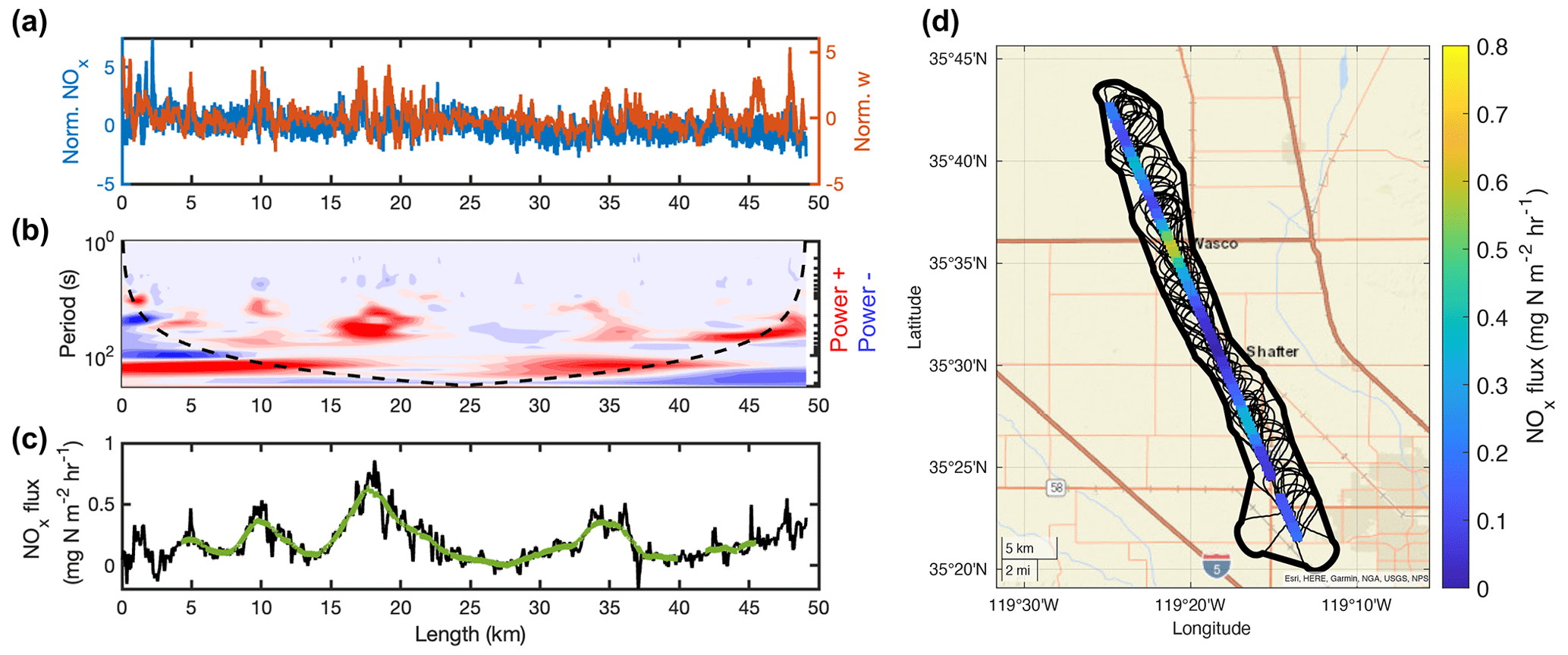
Figure 1 (a) The variance in the normalized NO_x and vertical wind speed. (b) Frequency and time-resolved wavelet power spectrum, with the cone of influence shown as a dotted black line. (c) The integrated fluxes from the raw data points are shown in black, and the fluxes after the moving average and COI filtering have been applied are shown in green. (d) The distribution map of flux resampled at 500 m. The black lines show the 90th percentiles of the footprints, and the thick black line denotes the contours of all footprints. Background map credits: Esri, HERE, Garmin, NGA, USGS, and NPS.

3.3 Footprint calculation

The footprint describes the contribution of surface regions to the observed airborne flux. We use the KL04-2D parameterization (Kljun et al., 2004) to calculate a space-resolved footprint map. This KL04-2D parameterization is developed from a 1-D backward Lagrangian stochastic particle dispersion model (Kljun et al., 2004). Metzger et al. (2012) implemented a Gaussian cross-wind distribution function to resolve the dispersion perpendicular to the main wind direction. The input parameters include the height of the measurements, standard deviation of the horizontal and vertical wind speed, horizontal wind direction, boundary layer height, surface roughness length, and friction velocity. We obtain the surface roughness length and friction velocity from the HRRR product. For each flux observation, we calculate the footprint map at the spatial resolution of 500 m and then extract the 90 % contour. Figure 1d depicts the 90 % KL04-2D footprint contours of observations resampled to 500 m in one segment. Each footprint contour is aligned with the horizontal wind direction and is transformed into a geographic coordinate space.

3.4 Filter out NO_x fluxes impacted by the off-road vehicle emissions

It is worth noting that croplands include not only soil NO_x emissions but also the off-road vehicle emissions. Erroneously attributing the NO_x from off-road vehicle emissions to soil NO_x emissions leads to a high bias. While trimethylbenzene was observed during RECAP-CA field campaign, Pfannerstill et al. (2023) presented the trimethylbenzene fluxes using the same algorithm described in Sect. 3.2. The trimethylbenzene fluxes are interpolated to match the NO_x fluxes in time and are utilized as an indicator of off-road vehicle emissions over croplands (Tsai et al., 2014). The trimethylbenzene fluxes are categorized into two groups; the first group presents footprints covering croplands exclusively, and the second group presents footprints with mixed land cover types. Shown in Fig. S9, the trimethylbenzene flux is much lower over croplands, with a median of 0.003 mg m⁻² h⁻¹ compared to a median of 0.009 mg m⁻² h⁻¹ over mixed land cover types, which includes highway and urban areas. No correlation between trimethylbenzene flux and NO_x flux is found over croplands. Among all observations over croplands, we identify those with trimethylbenzene fluxes larger than 0.02 mg m⁻² h⁻¹, which consist of 7 % of the total data points and are impacted by the off-road vehicle emissions, and then filter out them in the later analysis. We also vary the threshold of the trimethylbenzene flux between 0.005 and 0.04 mg m⁻² h⁻¹ and conclude that the choice of the threshold does not influence the results.

3.5 Vertical divergence

Extrapolating the airborne flux to surface flux should account for the vertical divergence. The vertical divergence is a result of multiple processes, including net in situ production or loss, storage, and horizontal advection.

To investigate the impact of vertical divergence, the flight route includes three vertically stacked racetracks during which the segments are close to each other in space but vary in height. After removing the legs that fail the quality control, only one racetrack measurement carried out between 14:20–15:10 LT on 8 June presented qualified flux segments, and the vertical distribution of fluxes is shown in Fig. S4. No consistent increase or decrease in the fluxes with increasing height is detected during the racetrack in this study because the vertical divergence is hampered by emissions heterogeneity. As shown in Fig. S7, the footprint map for each segment at various altitudes covers regions with high heterogeneity. Therefore, we use an alternative approach for calculating the vertical divergence. Instead of extracting racetrack measurements, we collect a subset of flux measurements during the whole field campaign based on the footprint coverage. Only fluxes with footprints covering croplands exclusively are included to avoid emissions heterogeneity. As shown in Fig. 2, we calculate the ratio of measurement heights relative to the PBL height ($z/z_i$), and 98 % of selected fluxes are located within 70 % of the PBL height and are divided into seven bins of $z/z_i$ with uniform width. We then perform a linear fit for the binned median fluxes versus $z/z_i$ to calculate the vertical correction factor $\left(C=\frac{\text{slope}}{\text{intercept}}\right)$. This correction factor is used to linearly extrapolated the fluxes at the measurement height (F_z) to fluxes at the surface (F₀) (Eq. 8). After the vertical divergence correction, the surface fluxes are on average 26 % higher than the fluxes at the measurement heights.

$$\begin{array}{}\text{(8)}& F_{\mathrm{0}}={\displaystyle \frac{F_x}{\mathrm{1}+C\frac{z}{z_i}}}\end{array}$$

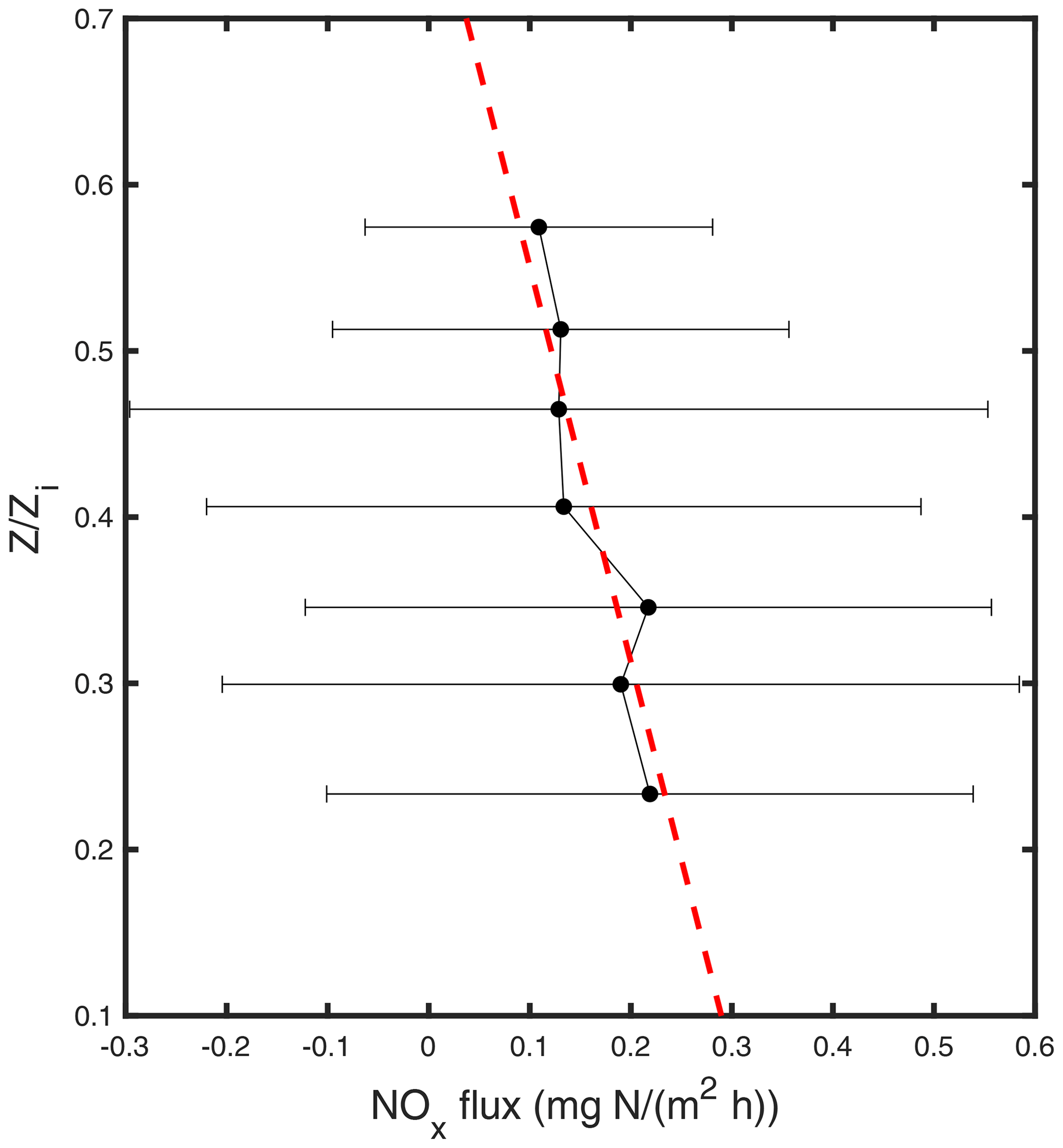
Figure 2 Vertical profiles of measured fluxes above croplands during RECAP-CA field campaign binned by the ratio of measurement height and PBL height ($z/z_i$). The points represent the median flux within each bin, and the error bars represent the standard deviation. The dashed red line shows a linear fit for median fluxes versus relative height.

3.6 Data qualify control and uncertainty analysis

The flux detection limit does not only depend on the signal-to-noise ratio of the NO_x measurement but also varies with wind speed and atmospheric stability. Following Langford et al. (2015), we calculate the limit of detection (LoD) of flux before the moving average and spatial average are applied. For each segment, the observed NO_x is replaced with a white noise time series and is then fed into the CWT to yield the corresponding time series of the noisy flux. The random error affecting the flux (${\mathit{\sigma }}_{{\mathrm{NO}}_x,\mathrm{noise}}$) is defined as the standard deviation of this noise-derived flux, and LoD is defined as 2$\times {\mathit{\sigma }}_{{\mathrm{NO}}_x,\mathrm{noise}}$ (95th confidence level). Among 142 segments, Fig. 3a shows the distribution of flux LoD among 142 segments. The LoDs range from 0.02 to 0.30 mg N m⁻² h⁻¹, and the average LoD is 0.10 mg N m⁻² h⁻¹. To obtain a better constraint on the flux quality, we compare the LoD against the time series of flux in each segment and filter out 18 segments in which the whole time series is below the LoD. The flux calculation using CWT introduces uncertainty from a variety of sources. We describe the systematic errors and random errors, following the work of Wolfe et al. (2018). Systematic errors arise from the undersampling of high-frequency and low-frequency ranges. The CWT algorithm fails to resolve a frequency higher than the Nyquist frequency. Due to the high temporal resolution (5 Hz), we expect a minimal loss at the high-frequency limit (Fig. S5). The upper limit of the systematic error associated with a low frequency is calculated using Eq. (9) (Lenschow et al., 1994).

$$\begin{array}{}\text{(9)}& \text{SE}\le \mathrm{2.2}{\left({\displaystyle \frac{z}{z_i}}\right)}^{\mathrm{0.5}}{\displaystyle \frac{z_i}{L}}\end{array}$$

z and L are the measurement heights and the length of segments, respectively. z_i values are the boundary layer heights from HRRR. We calculate the low-frequency error ranges from 1 % to 5 %.

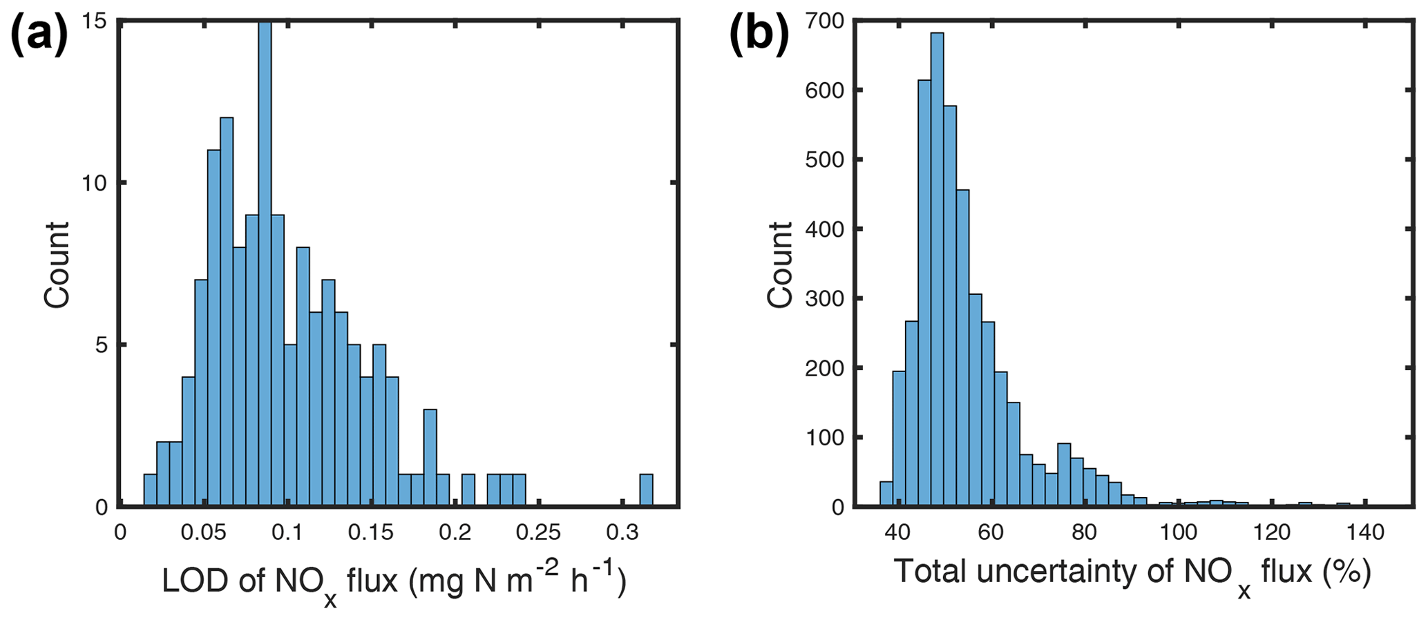
Figure 3 (a) The distribution of the segment-based NO_x flux detection limit (LoD). (b) The distribution of total uncertainty in the NO_x flux at 500 m spatial average.

Random errors arise from the noise in the instrument (RE_noise) and the noise in turbulence sampling (RE_turb), which are calculated using Eqs. (10) and (11) (Wolfe et al., 2018; Lenschow et al., 1994).

$$\begin{array}{}\text{(10)}& {\text{RE}}_{\mathrm{noise}}={\displaystyle \frac{\sqrt{{\mathit{\sigma }}_{{\mathrm{NO}}_x,\mathrm{noise}}^{\mathrm{2}}{\mathit{\sigma }}_{\mathrm{w}}^{\mathrm{2}}}}{N}}\end{array}$$

$$\begin{array}{}\text{(11)}& {\displaystyle \frac{{\text{RE}}_{\mathrm{turb}}}{F}}\le \mathrm{1.75}{\left({\displaystyle \frac{z}{z_i}}\right)}^{\mathrm{0.25}}{\left({\displaystyle \frac{z_i}{L}}\right)}^{\mathrm{0.5}}\end{array}$$

z, L, and z_i values are the same as Eq. (9), and ${\mathit{\sigma }}_{\mathrm{w}}^{\mathrm{2}}$ is the variance of the vertical wind speed. Note that RE_noise assumes that the noise in each time step is uncorrelated; therefore, we ignore the moving average step in the uncertainty calculation, and N denotes the number of points used to yield each 500 m spatially averaged flux.

Utilizing a constant lag time introduces an additional source of uncertainty. We estimate the uncertainty by comparing the calculated fluxes using segment-specific and constant lag times across all segments for which specific lag times are available. As shown in Fig. S4, the difference is less than 25 % for 90 % of the data. Therefore, we attribute an uncertainty of 25 % due to the lag time correction (RE_lag). While we believe that this error is unphysical and that a single lag time is more appropriate, we include it to be conservative in our estimate of the uncertainties.

Estimating the uncertainty caused by the correction of vertical divergence is tricky. While we conclude that the influence of vertical divergence is non-negligible, it has been ignored in some previous airborne flux studies (e.g., Vaughan et al., 2016; Hannun et al., 2020; Vaughan et al., 2021; Drysdale et al., 2022). While the flux is scattered in each vertical interval in our divergence calculation, we first bootstrap the flux observations and calculate the uncertainty in the correction factor (σ_C) to 40 %. As we see a significant difference in the vertical correction factor for racetrack measurements versus a selected subset of flux observations, we tentatively set the uncertainty of C to 100 % in order to account for the case of no vertical divergence. Besides, we account for a 30 % uncertainty in the PBL heights.

We propagate the total uncertainty from each component using Eq. (13), and the distribution of the total uncertainty of the 500 m average NO_x flux is shown in Fig. 3b. The average uncertainty is 60 %, and the interquartile of the total uncertainty is 48 % and 68 %. The random error and the vertical divergence correction dominate the uncertainty, and the uncertainty is consistent with previous studies (Wolfe et al., 2018; Vaughan et al., 2016).

$$\begin{array}{}\text{(12)}& {\displaystyle }{\mathit{\sigma }}_{F_z}=\sqrt{{\text{SE}}^{\mathrm{2}}+{\text{RE}}_{\mathrm{noise}}^{\mathrm{2}}+{\text{RE}}_{\mathrm{turb}}^{\mathrm{2}}+{\text{RE}}_{\mathrm{lag}}^{\mathrm{2}}}\text{(13)}& {\displaystyle }\begin{array}{rl}& {\mathit{\sigma }}_{F_{\mathrm{0}}}=\\ & \sqrt{{\displaystyle \frac{{\mathit{\sigma }}_{F_z}^{\mathrm{2}}}{{\left(\mathrm{1}+C\frac{z}{z_i}\right)}^{\mathrm{2}}}}+{\mathit{\sigma }}_C^{\mathrm{2}}{\left({\displaystyle \frac{z}{z_i}}\right)}^{\mathrm{2}}{\left({\displaystyle \frac{F_z}{{\left(\mathrm{1}+C\frac{z}{z_i}\right)}^{\mathrm{2}}}}\right)}^{\mathrm{2}}+{\mathit{\sigma }}_{z_i}^{\mathrm{2}}{\left({\displaystyle \frac{Cz}{z_i^{\mathrm{2}}}}\right)}^{\mathrm{2}}{\left({\displaystyle \frac{F_z}{{\left(\mathrm{1}+C\frac{z}{z_i}\right)}^{\mathrm{2}}}}\right)}^{\mathrm{2}}}\end{array}\end{array}$$

4 Component flux disaggregation

The overview of observed fluxes across seven flights over San Joaquin Valley is illustrated in Fig. 4. It shows a distinct spatial heterogeneity (Fig. 4a). For instance, high NO_x flux signals are detected when the aircraft was flying above highway 99 between Bakersfield and Visalia. The transect of cities, such as Fresno, captures a substantial enhancement of NO_x fluxes. Figure 4b exhibits the distribution of airborne fluxes. In total, 90 % of the fluxes are positive, demonstrating that our airborne flux measurements are capable of detecting NO_x emissions over the study domain. We attribute the remaining 10 % of negative fluxes to the uncertainties in the flux calculation. The distribution of observed fluxes is right-skewed; the mean and median observed flux over the SJV is 0.37 and 0.25 mg N m⁻² h⁻¹, respectively. The interquartile range of the flux is 0.11 and 0.49 mg N m⁻² h⁻¹. In total, 1.2 % of extremely high fluxes exceeding 2 mg N m⁻² h⁻¹ represents the long tail in the flux distribution, which is, like the negative fluxes, most likely caused by the incomplete sampling of the spectrum of eddies driving the fluxes.

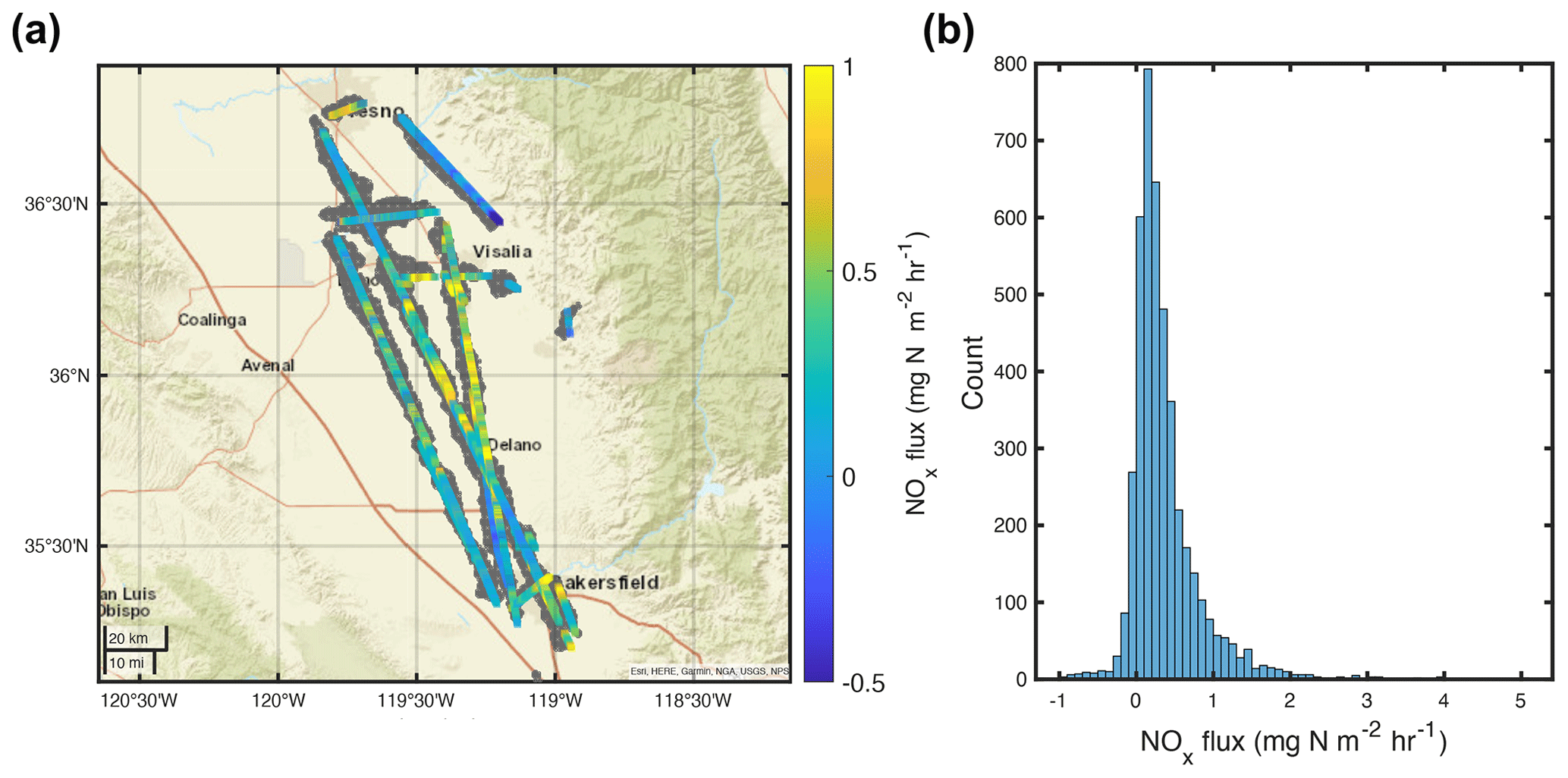
Figure 4 (a) The map of observed airborne fluxes over seven flights over the San Joaquin Valley. If the segments overlap each other, then the average flux is calculated. The gray shading represents the coverage of 90 % footprint extents for all flux observations. Background map credits: Esri, HERE, Garmin, NGA, USGS, and NPS. (b) The distribution of full data sets of observed airborne NO_x fluxes is shown.

As discussed in Sect. 3.3, we then calculate the footprint for each flux observation during the RECAP-CA field campaign. Figure 4a shows the 90 % footprint extent in gray. Figure S8 shows that the 90 % extent for the calculated footprints ranges from 0.16 to 12 km, with a mean extent of 2.8 km. The KL04-2D footprint algorithm has been applied to an airborne flux analysis over London, and in that study, the 90 % footprint extents range from 3 to 12 km from the measurement (Vaughan et al., 2021). While the largest footprint extent is comparable with those from Vaughan et al. (2021), our calculated footprints mostly have a smaller extent, as 62 % of the footprint extents are within 3 km of the aircraft flight track. We attribute the small footprints to the stagnant weather conditions and weaker horizontal wind advection compared to London. The mean wind speed is 2.9 m s⁻¹ for full observation data sets and 2.4 m s⁻¹ for those data points with footprint extents less than 3 km. The largest footprint extent corresponds to observations at the foothills, due to the higher altitude relative to the boundary layer height and stronger horizontal wind advection.

The region covered by the footprints is composed of mixed land cover types. We use the 2018 United States Department of Agriculture (USDA) CropScape database (https://nassgeodata.gmu.edu/CropScape/, last access: 24 August 2023) to describe the land cover types. The resolution has been degraded from the native 30 m resolution to 500 m. For each grid, the land cover type is assigned if a land type makes up more than 50 % of the 500 m grid cell. We generalize a “soil” land cover type if the land cover type is identified as being either croplands or grassland. The grids classified as “developed” in CropScape are dominated by anthropogenic activities, including transportation and fuel combustion. We overlay the national highway network and categorize the grids containing highways as “highway” land types. The remaining grids are classified as “urban”, and they correspond to the area with heavy populations in the absence of highways. The distinction between a “highway” and an “urban” land type is utilized to address on-road mobile sources. In total, 37 % of the flux observations include the highway land type in the 90 % footprint extent, 23 % of the observations include the urban land type, and 96 % of the observations include the cultivated soil land type.

To disentangle the flux emanating from different land cover types, we apply the Disaggregation combining Footprint analysis and Multivariate Regression (DFMR) methodology described in Hutjes et al. (2010). The observed fluxes are treated as the weighted sum of component fluxes from each land cover type as follows:

$$\begin{array}{}\text{(14)}& F_{\mathrm{obs}}=\sum _{k=\mathrm{1}}^{\mathrm{3}}{w}_k{F}_k,\end{array}$$

where k₁ to k₃ denote the highway, urban, and soil land types, w_k is the fractional area within the 90 % footprint contour, and F_k values are the corresponding component fluxes. The multi-linear regression is applied to observations from all flights, which consist of 4391 data points. We perform the Monte Carlo simulation to identify the uncertainty in the multi-linear regression due to the flux uncertainty. The resulting statistical uncertainty is shown in Fig. 5. The highway land type yields the highest flux of 0.96 mg N m⁻² h⁻¹, with a standard deviation of 0.04 mg N m⁻² h⁻¹. The areas classified as urban land type exhibit a flux of 0.43 (±0.02) mg N m⁻² h⁻¹, which is ∼ 50 % of the highway flux. Most likely, the fluxes from highway land types are even higher than 0.96 mg N m⁻² h⁻¹. Note that the land type map is at a 500 m spatial scale, so the grid classified as highway indeed includes both the highway and areas near the highway. If, for example, the highway is only 10 % of the true area of the land cover pixel, then the fluxes on the highway could be as much as 10 times larger. The cultivated soil land type flux of 0.30 (±0.01) mg N m⁻² h⁻¹ is large. It is about one-quarter the magnitude of the highway flux and half that of the urban flux. As the total area of soil pixels is much larger than the area of highway or urban pixels integrated across the SJV, cultivated soil NO_x emissions are a major factor.

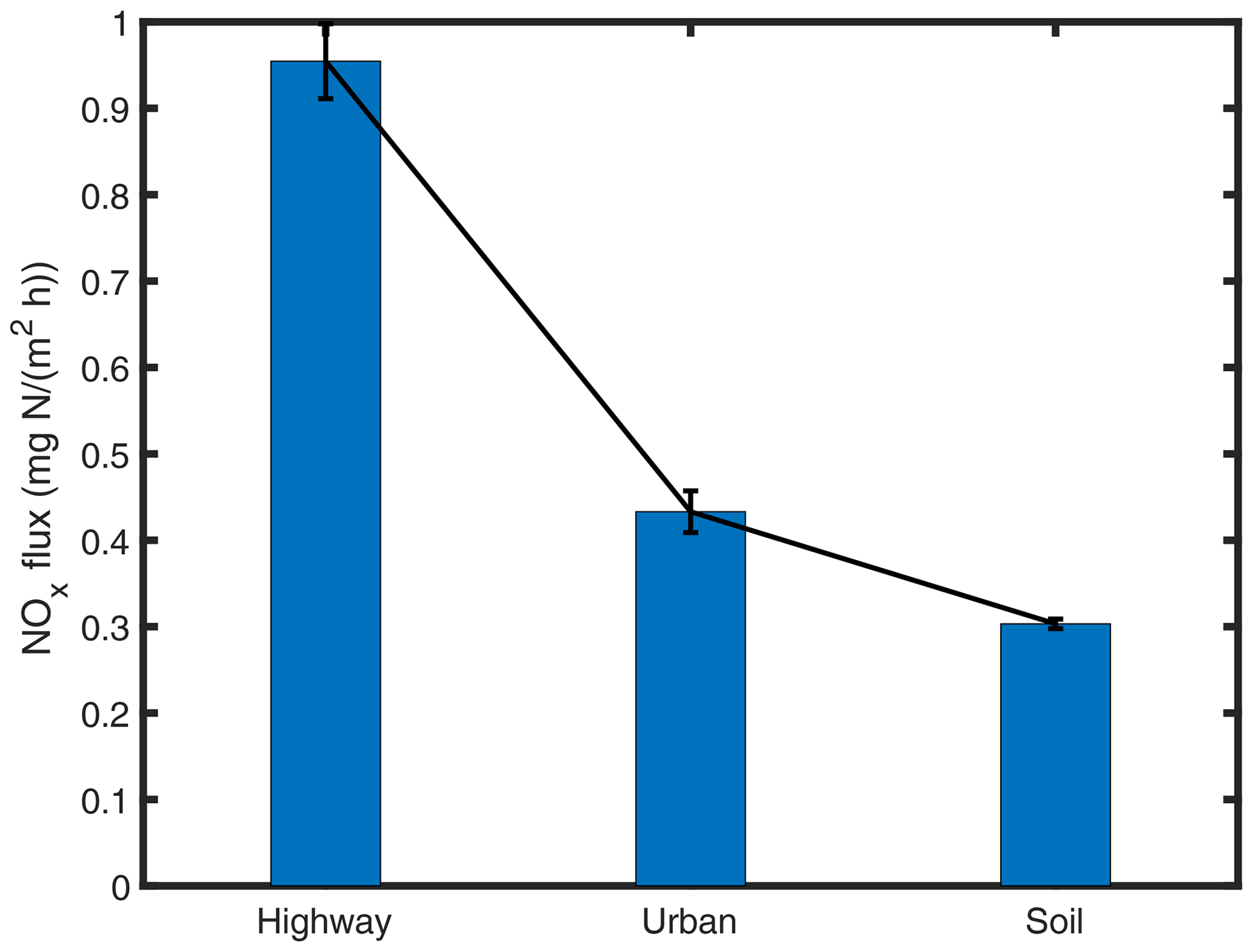
Figure 5 Bootstrapped statistical results of multi-linear regression to resolve component fluxes from the highway, urban, and cultivated soil land types. Each bar represents the average component fluxes from each land type, and the black line shows the standard deviation.

5 Calculation of NO_x emissions map using airborne NO_x fluxes

While these separate component fluxes emphasize the distinction between individual land types at the spatial resolution of the land cover (500 m), we utilize the NO_x fluxes to yield an estimate of NO_x emissions at 4 km. For each 4 km grid, we collect the observed fluxes for which 90 % of the footprint overlaps with this grid area and define the weight r_k as the fractional area that the footprint covers. The emissions (in units of mg N m⁻² h⁻¹) is calculated by the weighted average of the flux (Eq. 15). Only grids measured by at least five flux observations are considered in order to focus our attention on those pixels for which we have a statistically representative sample of the emissions.

$$\begin{array}{}\text{(15)}& {\text{Emis}}_i={\displaystyle \frac{{\sum }_{k=\mathrm{1}}^{n\ge \mathrm{5}}{r}_k{F}_k}{{\sum }_{k=\mathrm{1}}^{n\ge \mathrm{5}}{r}_k}}\end{array}$$

The emissions are calculated based on the observations from six flights during weekdays (Fig. 6a). The largest reported weekday emissions were on 3 June, when the median emissions were 0.39 mg N m⁻² h⁻¹. The lowest weekday emissions were observed on 15 June, with the median emissions of 0.14 mg N m⁻² h⁻¹. The large daily variation observed in estimated emissions during weekdays is partially due to the variation in flight routes and footprint coverage. This is illustrated by the daily estimated emissions map shown in Fig. S10.

As the emissions inventories make a distinction between weekdays and weekends and do not account for the daily variation on different weekdays, we average over the six weekday flights to yield the best estimate of emissions maps over the San Joaquin Valley derived from flux measurements (Fig. 6b). The median estimated weekday NO_x emissions over the study domain is 0.26 mg N m⁻² h⁻¹, with an interquartile range of 0.14 and 0.46 mg N m⁻² h⁻¹. The observed emissions map describes high NO_x emissions in the cities of Bakersfield (35.3^∘ N, 119^∘ W) and Fresno (36.75^∘ N, 119.8^∘ W) and along highway 99.

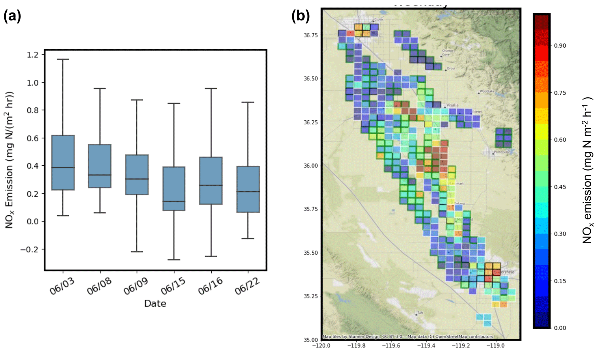
Figure 6 (a) The box-and-whisker plot of observed emissions for each flight, aligned according to the order of the flight days. The box represents the interquartile ranges of observed emissions, and the line represents the median emissions. The whiskers show the maximum and minimum values. (b) The spatial distribution of emissions at 4 km over SJV as derived from observed fluxes during weekdays. The patch color shows the observed NO_x emissions. The edge color denotes the land cover type, with the grid cells covering highways in white and those covering urban regions in black, and the rest of the grid cells are categorized with cultivated soil land cover types in green. © OpenStreetMap contributors 2022. Distributed under the Open Data Commons Open Database License (ODbL) v1.0.

5.1 Evaluation of anthropogenic NO_x emissions inventories

First, we compare the observations to the inventory developed by the California Air Resources Board (CARB). The anthropogenic emissions of NO_x consist of mobile sources, stationary sources, and other NO_x emissions from miscellaneous processes such as residential fuel combustion and managed disposal. In the CARB inventory, the mobile sources are estimated from the EMission FACtors (EMFAC) model, v1.0.2 (CARB, 2021a), and the Off-Road mobile source emissions model (CARB, 2021b). The stationary sources are estimated based on the reported survey of facilities within each local jurisdiction and the emissions factors from the California Air Toxics Emission Factor (CATEF) database (CARB, 2021c). Hereinafter, we utilize “EMFAC” to represent anthropogenic vehicle-related NO_x emissions used in the CARB inventory. An alternative anthropogenic emissions inventory is the Fuel-Based Inventory for Vehicle Emissions (FIVE), developed by McDonald et al. (2012) and updated by Harkins et al. (2021). Both emissions inventories are at 4 km spatial resolution.

To disentangle the contribution of different NO_x emissions sources, we attribute emissions at grid cells covering either highway or urban regions to anthropogenic emissions from transportation and fuel combustion, and those at remaining grid cells are categorized as soil NO_x emissions. For each grid cell categorized as being dominant in anthropogenic emissions, we then match the emissions inventories representing the weekday scenario to the same hour and grids of emissions derived from measured fluxes. The corresponding hour of the estimated emissions is rounded to the closest hour of the observation times. Figures 7 and S12 show the comparison of observed anthropogenic emissions against EMFAC and FIVE emissions inventories. Over urban regions, the mean and median observed RECAP-CA NO_x emissions are 0.37 mg N m⁻² h⁻¹, and the interquartile range is 0.14 and 0.58 mg N m⁻² h⁻¹. Both EMFAC and FIVE yield a good agreement with our measurements; the mean urban NO_x emissions are 0.40 and 0.43 mg N m⁻² h⁻¹. However, the median urban NO_x emissions in these inventories is 24 % and 22 % lower than the observation, respectively. The estimated NO_x emissions on grid cells covering highways are more scattered. The median estimated NO_x emissions is 0.24 mg N m⁻² h⁻¹. It is lower than on urban grid cells due to spatial averaging and due to the fact that most of the highway length is outside of the urban regions. The distribution of observed RECAP-CA NO_x emissions from the highway is right-skewed and characterized by an interquartile range of 0.14 and 0.47 mg N m⁻² h⁻¹. We also note that over highway 99, the RECAP-CA NO_x emissions are a factor of 3 higher than average on grid cells near congestion, reflecting the variation in the emissions caused by real-time traffic conditions. Both EMFAC and FIVE provide lower NO_x emissions over highway grids; the median NO_x emissions are 37 % and 50 % of those from the RECAP-CA observations. The highway pixels include land cover that is mostly non-highway and typically soil. If soil N emissions are substantially larger than in these inventories, then it is possible that the measurements and bottom-up inventories for highways are in better agreement than indicated by the figure.

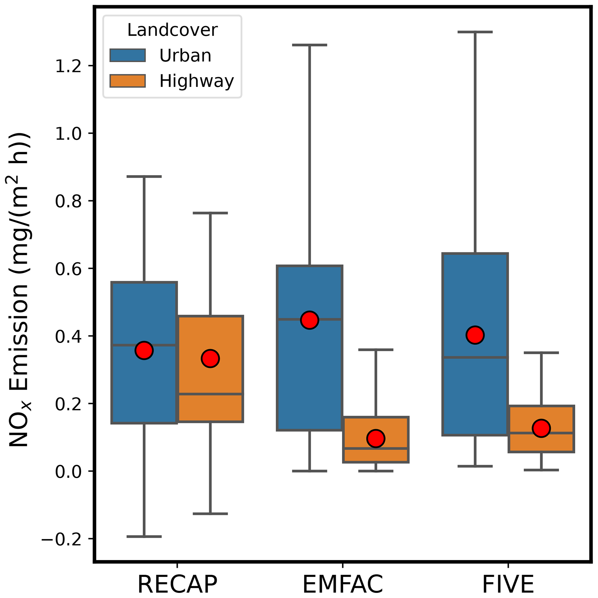
Figure 7 The box-and-whisker plot of observed RECAP-CA anthropogenic NO_x emissions from transportation and fuel combustion, as well as those from EMFAC and FIVE emissions inventories, separated by highway and urban land cover types. The box is the interquartile range with the line of the median value. The maximum and minimum emissions are shown by whiskers, and the mean emissions are shown in red dots.

5.2 Evaluation of soil NO_x scheme

Soil NO_x emissions are determined by biogeochemical processes, including soil microbe‐mediated nitrification and denitrification. Process‐based biogeochemical models have been developed to mechanistically represent soil NO_x emissions by simulating nitrogen interactions in ecological systems, such as DeNitrification‐-DeComposition (DNDC; Li et al., 1992, 1994; Guo et al., 2020) and DAYCENT (Del Grosso et al., 2000; Rasool et al., 2019). However, these process-level models are not yet widely applied to chemical transport models, and the default model configuration uses empirical soil NO_x schemes. The Model of Emissions of Gases and Aerosols from Nature v3 (MEGAN; Guenther et al., 2012) is the most commonly used scheme and is used to predict soil NO_x emissions in the CARB emissions inventory. It is gridded at a 4 km spatial scale and has hourly time steps. The Biogenic Emission Inventory System (BEIS) is the default scheme to estimate volatile organic compounds from vegetation and NO from soil, as developed by the United States Environmental Protection Agency (EPA). We obtain the hourly BEIS v2.14 soil NO_x emissions at 4 km during the study period from the Weather Research and Forecasting model coupled with Chemistry (WRF-Chem), using the same model configuration described in Kim et al. (2022). While soil NO_x varies nonlinearly with meteorological conditions, soil conditions, and agricultural activities, both MEGAN and BEIS simplify the nonlinearity to an activity factor (γ), as a function of ambient temperature, leaf area index, and leaf age. A recently developed soil NO_x scheme, the Berkeley–Dalhousie–Iowa Soil NO Parameterization (BDISNP; Hudman et al., 2012; Sha et al., 2021), is an intermediate complexity model and includes more details than the other two in order to be more faithful to direct measurements made at soils and to describe their seasonal and hourly variations. The BDISNP model includes parameters representing the effects of soil moisture, temperature, and soil nitrogen, including fertilizer. Using the same WRF-Chem setup described in Sha et al. (2021), we also calculate the BDISNP soil NO_x emissions during the study period at the spatial resolution of 2 km and regrid them to 4 km.

Figure 8a illustrates the range of soil N emissions derived from RECAP-CA observations, as compared to these three different soil NO_x schemes. The analysis of the observations exhibits median cultivated soil NO_x emissions of 0.26 mg N m⁻² h⁻¹; the interquartile range of the inferred emissions is 0.14 and 0.45 mg N m⁻² h⁻¹. MEGAN and BEIS both have emissions an order of magnitude lower, with median soil NO_x emissions of 0.008 and 0.011 mg N m⁻² h⁻¹, respectively. The BDISNP soil NO_x scheme shows median soil NO_x emissions of 0.14 mg N m⁻² h⁻¹. Figure 8b exhibits a point-by-point comparison of the observed RECAP-CA and the BDISNP soil NO_x emissions, showing that there is a correspondence between the two, but the model is 2.2 times lower than the observations. Figure S13a and d show the spatial distribution of soil NO_x emissions from observation and BDISNP scheme. Both show higher soil NO_x emissions between 35.75 and 36.25^∘ N.

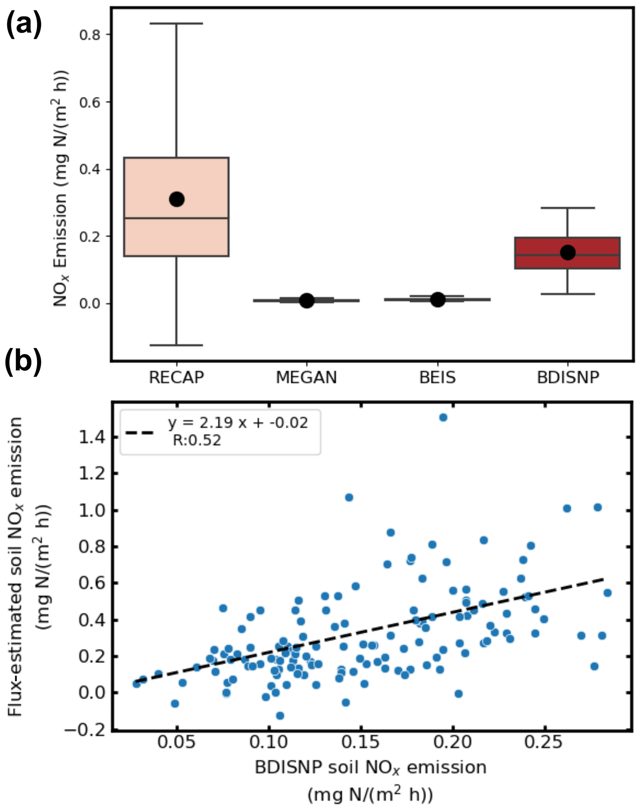
Figure 8 (a) The box-and-whisker plot of observed soil NO_x emissions and parameterized soil NO_x emissions from MEGAN, BEIS, and BDISNP schemes. The mean soil NO_x emissions are shown in black dots. (b) The scatterplot of soil NO_x emissions calculated from BDISNP scheme and from flux measurements. The dashed black is the least square linear fit.

A distinct characteristic of soil NO_x emissions is its temperature dependence. For instance, Oikawa et al. (2015) identified unusually high soil NO_x emissions in a high-temperature agricultural region based on in situ observations. The temperature-driven increase in soil NO_x emissions raises concerns in the future warmer climate, resulting in a larger contribution to O₃ pollution (Romer et al., 2018). Here we leverage our flux observations to probe this temperature dependence, as shown in Fig. 9. We collect observed NO_x emissions for each flight and select the subset of NO_x emissions on grids categorized as cultivated soil land type. We also collect corresponding mean soil temperature from WRF-Chem and match them to observed NO_x emissions both in time and space. A range of soil temperature between 295 and 304 K is observed. We apply the linear regression fit between soil temperature and estimated soil NO_x emissions and show a positive temperature dependence of soil NO_x emissions with the slope of 0.02 (±0.008) mg N m⁻² h⁻¹ K⁻¹. We then bin observed soil NO_x emissions to three soil temperature categories, each of which has 2 K intervals. The median soil NO_x emissions increase from 0.22 to 0.29 mg N m⁻² h⁻¹, with the median soil temperature increasing from 296 to 300 K. As the response to soil temperature is incorporated in the BDISNP scheme, we also bin the BDISNP parameterized soil NO_x emissions into the same soil temperature categories. Both the RECAP-CA-measured flux and the BDISNP-modeled soil NO_x emissions exhibit an approximately 33 % increase over the range of soil temperature shown.

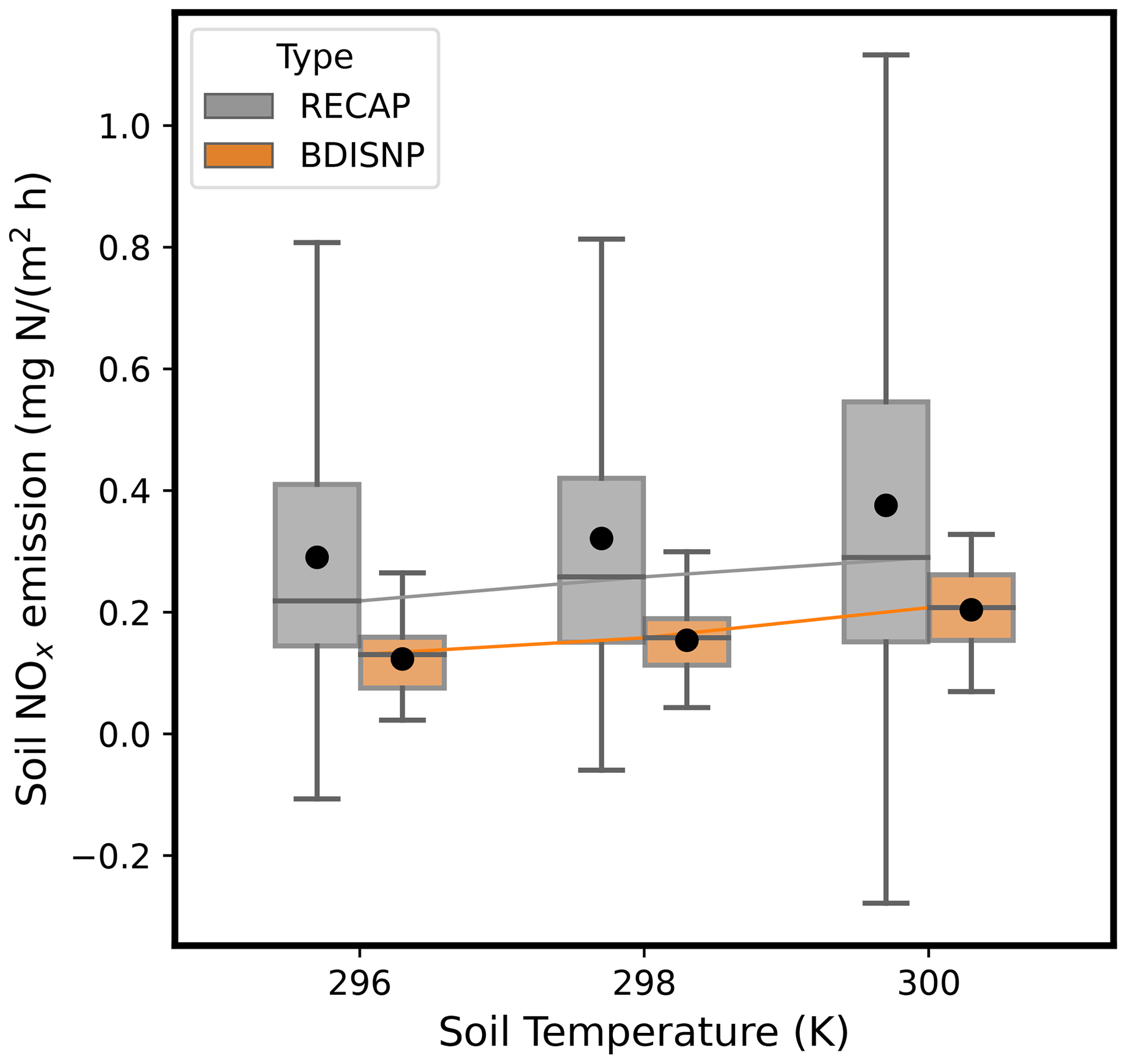
Figure 9 The dependence of soil NO_x emissions on soil temperature from both the flux measurements (gray) and BDISNP scheme (orange). Both observed and BDISNP soil NO_x emissions are binned, based on mean soil temperature from WRF-Chem. Three soil temperature bins are described with 4 K intervals. The box-and-whisker plot shows the distribution, and the black dot shows the mean within each bin. The line connects the median soil NO_x emissions across three bins.

5.3 Discussion of soil NO_x emissions

Soil NO_x emissions in California have been studied in field experiments. Matson et al. (1997) measured soil NO_x emissions from nine dominant crop types in SJV and reported mean fluxes of 0.01–0.09 mg N m⁻² h⁻¹. They also reported a large variation in the measured NO_x flux among crops and among different fields of the same crop; the highest measured NO_x flux is 0.17 mg N m⁻² h⁻¹, due to the fertilizer application and soil moisture characteristics. Horwath and Burger (2013) observed an average flux of 0.05–0.28 mg N m⁻² h⁻¹ at middays during the summertime from five crops in California, and the highest NO_x flux is >4 mg N m⁻² h⁻¹ in systems receiving large N inputs, which results in high concentrations of ammonium. Oikawa et al. (2015) observed soil NO_x emissions in a high-temperature fertilized agricultural region of the Imperial Valley, CA, ranging between −0.02 and 3.2 mg N m⁻² h⁻¹. They also conducted control experiments to investigate the soil NO_x emissions response to fertilization and irrigation. The highest soil NO_x flux was reported ∼10 d after the fertilizer at the soil volumetric water content of 30 % and a soil temperature of ∼313 K.

The mean soil NO_x flux, 0.32 mg N m⁻² h⁻¹, derived in our flux measurements is higher than the mean fluxes reported in Matson et al. (1997) and Horwath and Burger (2013); however, the range of estimated soil NO_x flux is within those in Horwath and Burger (2013) and Oikawa et al. (2015). Fertilizer is likely the primary contributor to the higher mean soil NO_x flux in our study. The RECAP-CA field campaign was conducted in June, right after the month of peak fertilizer use in SJV (Guo et al., 2020). As shown in Oikawa et al. (2015), the soil NO_x flux can increase up to 5-fold within 20 d of fertilizer. The higher mean soil NO_x flux is also contributed by higher soil temperature. In our study, the mean soil temperature is 299 K, with a range between 295 and 304 K, whereas the observations in Horwath and Burger (2013) and Oikawa et al. (2015) spread over a wider range of soil temperature (288–315 K). Consistent with our study, the temperature dependence of the soil NO_x emissions is observed in these field experiments. Horwath and Burger (2013) reported a 2.5–3.5-fold increase in NO_x fluxes with a 10 ^∘C increase in soil temperature. Oikawa et al. (2015) showed that the temperature dependence of soil NO_x emissions is nonlinear; a steeper increase in soil NO_x emissions was observed with the soil temperature exceeding 295 K.

It is worth noting the limitation of estimated soil NO_x emissions in our study. First of all, we are unable to investigate the dependence of soil NO_x emissions on meteorological drivers other than soil temperature, such as soil moisture, as modeled soil moisture presents a very small variation during the field campaign. Second, as our measurements only cover limited cropland areas in SJV over a short time period, and it is around the time of fertilizer use, we cannot scale the estimated soil NO_x emissions to the whole year or to the total cropland areas in California. Therefore, we cannot directly compare our estimate of soil NO_x emissions against other studies reporting soil NO_x emissions on an annual basis or on a larger spatial scale. Last, in the absence of ozone and PM_2.5 observations, we cannot investigate the impact of soil NO_x emissions on air quality. However, as the SJV is in the NO_x-limited regime (Pusede et al., 2014), we expect that a model that captures the soil NO_x more accurately will produce higher ozone. Future work is needed to further advance our understanding of soil NO_x emissions and their role in urban and rural air pollution.

6 Conclusions

We performed airborne NO_x flux measurements during RECAP-CA field campaign over the San Joaquin Valley. Seven flights were made over the SJV in June 2021. When combined with footprint and land cover information, we resolved the spatial heterogeneity in landscape flux. The component fluxes are estimated based on the multi-linear regression and exhibit statistically significant differences. The component fluxes are the highest from highways at 0.96 mg N m⁻² h⁻¹. Cultivated soil land types emit a non-negligible flux of 0.30 mg N m⁻² h⁻¹. The airborne flux observations are projected to a 4 km grid spacing to yield an estimated emissions map over the SJV. We utilize this map to evaluate emissions inventories commonly used in photochemical modeling. The anthropogenic emissions inventories, EMFAC and FIVE, agree well with the estimated mean NO_x emissions over urban regions. However, the widely used, but not biogeochemical-process-based, models for soil NO_x emissions underestimate emissions by an order of magnitude or more in the SJV, leading to a poor assessment of the relative roles of mobile and agriculture sources of NO_x in the region. The BDISNP model, as adapted by Sha et al. (2021), results in a better comparison with the observations. Even though it is still lower by a factor of 2, we show that it yields a similar spatial pattern and soil temperature dependence, as observed. Variations in this model are embedded in CMAQ (Rasool et al., 2019) and GEOS-CHEM (Wang et al., 2021) and have been implemented in WRF-CHEM by Sha et al. (2021). Studies in which soil NO_x is potentially important should make use of these codes, all of which are more consistent with observations at multiple scales.