the Creative Commons Attribution 4.0 License.
the Creative Commons Attribution 4.0 License.
 | 30 Aug 2023
Technical note: On HALOE stratospheric water vapor variations and trends at Boulder, Colorado
This study compares time series of stratospheric water vapor (SWV) data at 30 and 50 hPa from 1993 to 2005, based on sets of Halogen Occultation Experiment (HALOE) profiles above the region of Boulder, CO (40∘ N, 255∘ E), and on local frost-point hygrometer (FPH) measurements. Their differing trends herein agree with most of the previously published findings. FPH trends are presumed to be accurate within their data uncertainties, and there are no known measurement biases affecting the HALOE trends. However, the seasonal sampling from HALOE is deficient at 40∘ N from 2001 to 2005, especially during late winter and springtime, when HALOE SWV time series at 55∘ N clearly show a springtime maximum. This study finds that the SWV trends from HALOE and FPH measurements nearly agree within uncertainties at 30 hPa for the more limited time span of 1993 to 2002. Yet, HALOE SWV at 50 hPa has significant and perhaps uncertain corrections for interfering aerosols from 1992 to 1994. Northern Hemisphere time series and daily SWV plots near 30 hPa from the Limb Infrared Monitor of the Stratosphere (LIMS) experiment indicate that there is transport of filaments of high SWV from polar to middle latitudes during dynamically active winter and springtime periods. Although FPH measurements sense SWV variations at all scales, the HALOE time series do not resolve smaller-scale structures because its time series data are based on an average of four or more occultations within a finite latitude–longitude sector. It is concluded that the variations and trends of HALOE SWV are reasonable at 40∘ N and 30 hPa from 1993 to 2002 and in accord with the spatial scales of its measurements and sampling frequencies.
- Article
(9230 KB) - Full-text XML
- BibTeX
- EndNote


There have been numerous studies of long-term changes of stratospheric water vapor (SWV) mixing ratios (e.g., Konopka et al., 2022; Hegglin et al., 2014; Hurst et al., 2011). SWV trends in the lowermost stratosphere are affected mainly by non-zonal variations of the cold-point temperature (CPT) at the tropical tropopause, followed by transport of the associated relatively dry, entry-level air. Hegglin et al. (2014) also report on the roles of the oxidation of methane to water vapor in the middle and upper stratosphere and on the impact of changes in the Brewer–Dobson circulation (BDC) on water vapor trends throughout the stratosphere. One remaining puzzle is that the SWV trends from frost-point hygrometer (FPH) measurements above Boulder, CO, are more positive (or less negative) than zonal-average and Boulder region analyses of SWV from the Halogen Occultation Experiment (HALOE) (Scherer et al., 2008). Lossow et al. (2018) reported that those differences increase with altitude, and they cautioned that trends over Boulder may not be representative of zonal-mean values some years. Konopka et al. (2022) found from reanalysis data that there is a moistening above the Boulder region during late boreal winter and spring.
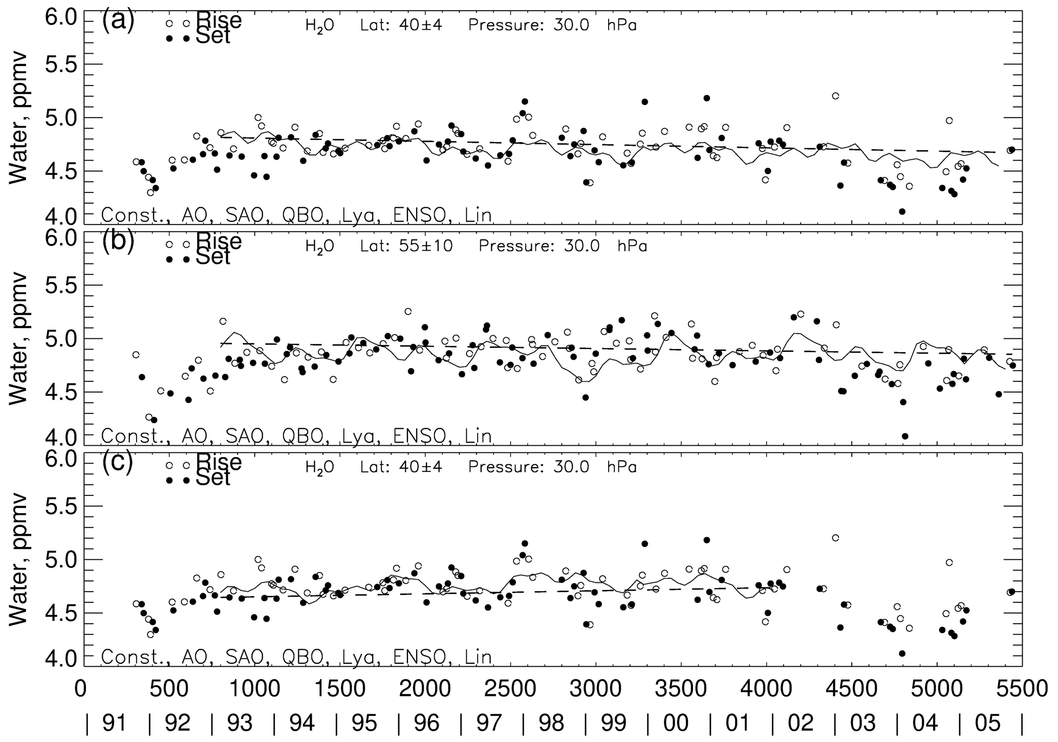
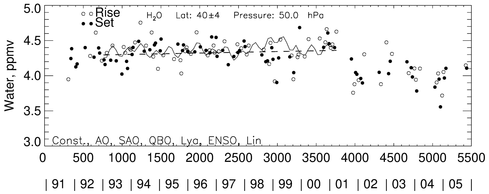
Figure 1MLR fit to a HALOE SWV time series: (a) Boulder sector, 40∘ N, 1993–2005; (b) at 55∘ N, 1993–2005; and (c) 40∘ N, 1993–2002. The fit of all the MLR terms is the oscillating curve; the linear trend term is the straight dashed line. Time by year or in days on the abscissa begins on 1 January 1991.
The present study reconsiders the HALOE SWV trends and variations near Boulder for 1993 through 2005 in Sect. 2 and compares them in Sect. 3 with those from the Boulder FPH measurements that are assumed to be accurate. The focus is on the trend differences at 30 hPa, where Lossow et al. (2018) found that they were largest. Section 4 reports on the SWV trend differences for the same years at 50 hPa or where there may be biases in HALOE SWV from its corrections for interfering aerosols. Section 5 shows a time series of Northern Hemisphere SWV near 30 hPa from the Nimbus 7 Limb Infrared Monitor of the Stratosphere (LIMS) dataset of 1978–1979. Daily plots of LIMS geopotential height (GPH) and SWV show the effects of meridional transport of SWV to 40∘ N during a dynamically active period in February 1979. That example provides evidence of a late-winter to spring moistening in the Boulder region. There are also instances of elevated SWV in the HALOE time series at subpolar latitudes at that time of year. Section 6 concludes that the HALOE SWV variations and trends at 40∘ N are understandable compared with those from FPH, given the spatial scales of their measurements, the reduction in sampling by HALOE after 2001, and possible HALOE SWV biases from interfering aerosols.
SWV time series from the HALOE dataset are analyzed by multiple linear regression (MLR) techniques in the manner of Remsberg (2008) and Remsberg et al. (2018a). Although HALOE began operations in October 1991, its SWV profiles are degraded in the lower stratosphere in 1991 through mid-1992 because of solar tracking anomalies in the presence of the very large extinction effects from Pinatubo aerosols. Figure 1a shows HALOE time series data from late 1991 through 2005 for the Boulder sector.
The Boulder region HALOE SWV points of Fig. 1a are for 30 hPa and are based on averages of profiles within the latitude range of 40±4∘ N and the longitude range of 255±35∘ E, since HALOE seldom measured profiles at the exact location of Boulder. A rather narrow latitude range was chosen for this study because there is a significant latitudinal gradient in SWV near 40∘ N in both fall and springtime. The finite longitude range of ±35∘ attains four or more profiles, between sunrise (SR) and sunset (SS) orbital crossings near Boulder, and it is sufficient for indicating low zonal wavenumber effects on the SWV field. The data in Fig. 1a from January 1993 onward are fit with an MLR model that corrects for effects of lag-1 autoregression (AR1) and accounts for memory between adjacent data points (Tiao et al., 1990); its AR1 coefficient is 0.35. The MLR model fit to the data of January 1993 through 2005 (solid curve) includes constant and linear trend terms as well as periodic annual (AO), semiannual (SAO), and quasi-biennial oscillation (QBO)-like terms. The periodic QBO-like term is approximated as a 28-month cycle, based on a Fourier analysis of an initial time series residual after accounting for the seasonal terms. The model also contains proxy terms for El Niño–Southern Oscillation (ENSO) forcings and solar cycle flux forcings. Significant terms are SAO, QBO-like, and ENSO proxy; the latter two terms account for differences from the fit of the HALOE data in Fig. 1a versus that from a simple seasonal fitting. The dashed line in Fig. 1a represents the sum of the constant term (4.84 ppmv) and a linear trend coefficient of ppmv per decade, having a confidence interval (CI) of 95 % or a trend of (2σ) % per decade. The SWV trend from Fig. 1a agrees closely with previous trends from HALOE data near 30 hPa in the latitude range of 35 to 45∘ N (Davis et al., 2016; Lossow et al., 2018).
All MLR term coefficients are reasonably accurate, if the seasonal sampling is good. However, from 2001 through 2005 there are few to no SR or SS samples in Fig. 1a from late winter through springtime. That sampling deficit became longer because HALOE was turned off a bit earlier prior to an Upper Atmosphere Research Satellite (UARS) yaw maneuver and then turned on later following the yaw event starting in 2001, to conserve power on the UARS spacecraft. While that change in operating procedure accounts for the lack of HALOE measurements near 40∘ N during late winter and springtime, the HALOE sampling frequency remains as prior to 2001 for lower- and higher-latitude zones. As an example, HALOE SWV for the longitude sector of Boulder but at the higher-latitude zone of 55±10 ∘N is in Fig. 1b and shows that the seasonal sampling occurs more regularly compared to that at 40∘ N in Fig. 1a. Northern Hemisphere SWV attains its annual maximum in late winter or early springtime, according to the MLR modeling of HALOE SWV at 55∘ N (Fig. 1b). Note that HALOE SWV at 55∘ N also has rather high values in early 2002 or following stratospheric warming events in the winter of 2001–2002 (Charlton and Polvani, 2007). There may have been transport of higher SWV values to 40∘ N that HALOE did not observe.
Separate MLR analyses of the SS and then the SR data points of Fig. 1a from 1993 to 2005 (not shown) yield trends that are significantly more negative for SS (−0.30 ppmv per decade) than for SR (−0.17 ppmv per decade). The HALOE SWV trends at 40∘ N for the time segment from 2001 to 2005 differ because of the timing of and/or lack of their late-winter and springtime values. Even so, it is expected that there ought to be decreasing SWV values at 40∘ N during those years in response to the decrease in SWV in the tropical lower stratosphere in early 2001, as noted by Randel et al. (2006), Scherer et al. (2008), Hegglin et al. (2014), and Konopka et al. (2022). They reported that there was a slight delay for a decrease in SWV at 40∘ N because of the slow ascent of the dry, tropical air as well as the subsequent meridional transport and mixing of that air to middle latitudes.
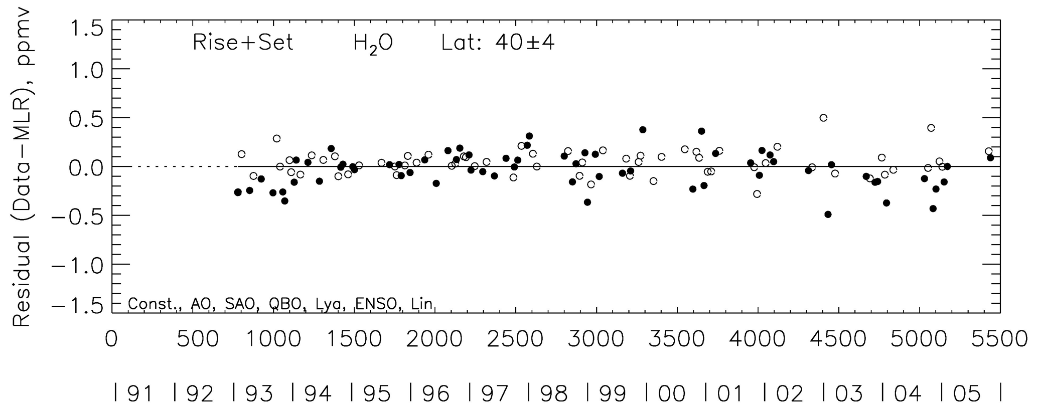
Scherer et al. (2008) noted that it is perhaps more appropriate to apply two piecewise linear trend terms for the MLR modeling of the HALOE SWV data in Fig. 1a, where there is a break point in 2002. Thus, Fig. 1c shows a separate trend analysis of HALOE SWV for the Boulder sector at 40∘ N but only for 1993 to 2002; its average SWV value is 4.62 ppmv, and its shorter trend term is no longer negative but positive at 0.22±0.04 ppmv per decade (or 4.7±0.7 (2σ) % per decade). Finally, Fig. 2 is the residual (data-minus-MLR model curve) for the fit in Fig. 1a, and its variations about the mean are of order ±0.3 ppmv. An important test of the adequacy of the set of terms in its MLR model is whether any structure remains in the residual. No periodic structure is apparent in Fig. 2, although there are clear seasonal gaps in the data series after 2001.
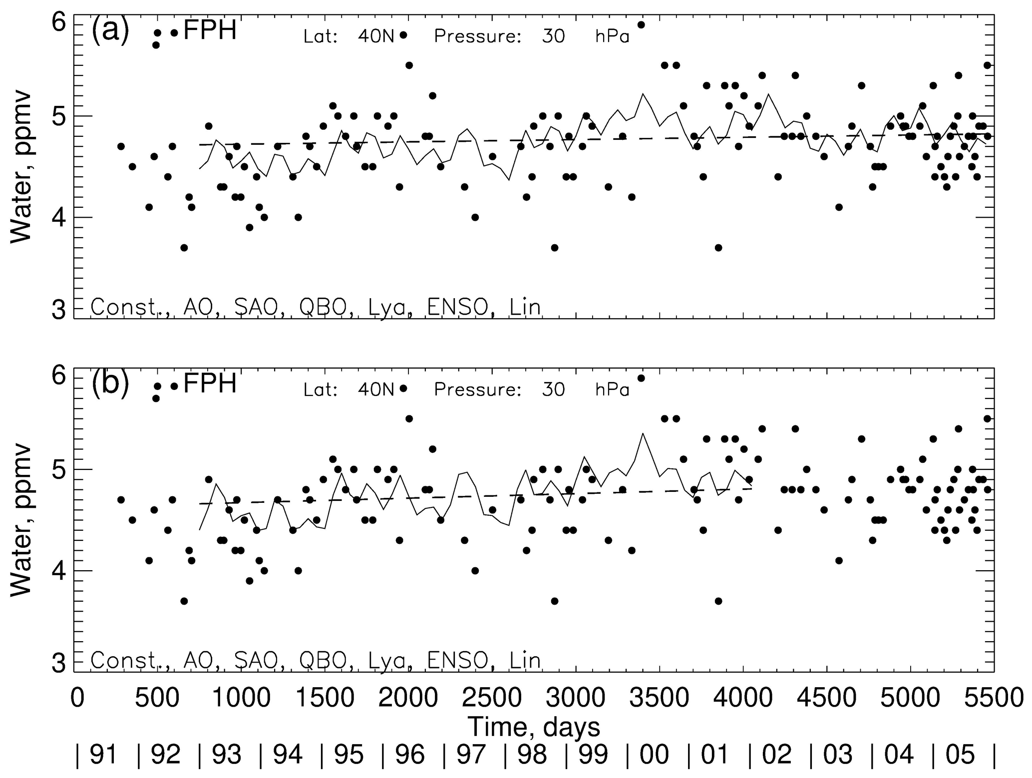
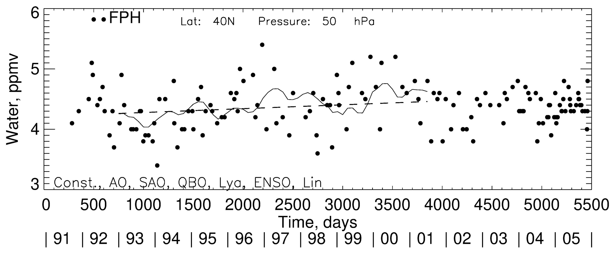
Figure 3Time series of FPH data and the MLR fit to them for comparison with Fig. 1: (a) 1993–2005 and (b) 1993–2002.
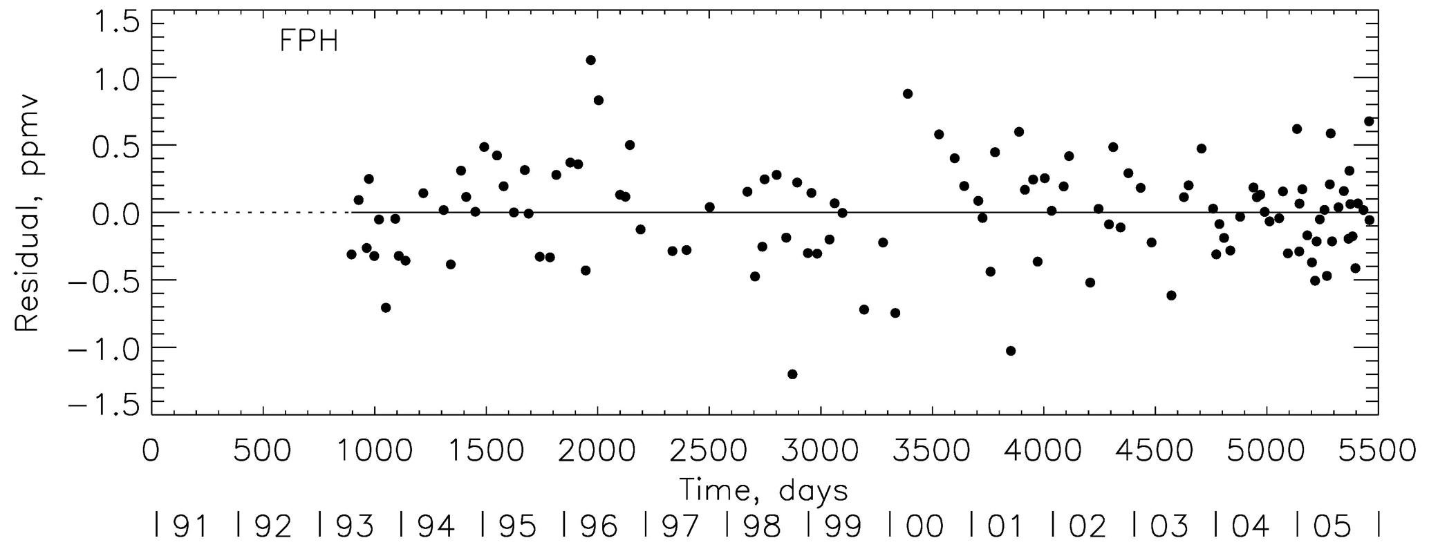
Figure 3a shows the SWV time series at 30 hPa from the FPH data at Boulder and for 1993–2005 for comparison with Fig. 1a. Individual FPH profiles were interpolated vertically to obtain SWV values at the 30 hPa level, and the FPH time series points are also spaced irregularly. SAO, QBO, ENSO, and linear terms from the MLR model of Fig. 3a have a significance of better than 90 %. The constant term is 4.70 ppmv, which is a bit less than that from the HALOE series (4.84 ppmv) but within the estimated systematic uncertainties for both measurements. The FPH trend for 1993–2005 is positive or ppmv per decade (or (2σ) % per decade), as compared to the negative trend from HALOE ( (2σ) % per decade). There is also a change in trend around 2002 in the FPH data of Fig. 3a, although it is not so apparent because of the rather large scatter of the FPH points. Figure 3b shows the corresponding FPH MLR analysis for 1993 to 2002, which yields an average SWV of 4.62 ppmv and agrees with the average HALOE value from Fig. 1c. The FPH trend for 1993 to 2002 is ppmv per decade (or % per decade), which is more positive than that of HALOE ( % per decade) but only slightly outside the overlapping envelope (e.g., +5.7 % per decade versus +5.4 % per decade) from their mutual trend uncertainties.
Figure 4 shows the residual (FPH minus MLR) for the time series data of Fig. 3a, where the FPH points exhibit more scatter compared with the HALOE residual in Fig. 2. Data points of the FPH record are assumed to be valid and accurate to <6 % or about ±0.3 ppmv, according to the extensive studies of Hall et al. (2016). The rather large scatter in Fig. 4 exceeds that uncertainty. Local FPH measurements are sensitive to SWV variations across all spatial scales. Note that the structure in the FPH residual of Fig. 4 is aperiodic and presumably due to small-scale atmospheric variations in some instances. Accordingly, it is difficult for the MLR modeling to fit all the real structure in the FPH data, and its linear trend term is not highly significant. Conversely, each individual HALOE profile gives an SWV value that is an average across its tangent view path (∼300 km) and with a vertical resolution of no better than 2 km. The HALOE time series points are also based on sector averages of four or more profiles. Thus, HALOE does not resolve SWV variations at small to intermediate scales.
There are high FPH SWV values in Fig. 3 on 22 May (5.8 ppmv) and on 26 June 1996 (5.5 ppmv), possibly due to elevated SWV in filaments of polar vortex air that were transported to and remained isolated above the location of Boulder for days to weeks (e.g., Manney et al., 2022). A search of individual profiles from HALOE reveals SWV values of order 6.5 ppmv at 60∘ N, 270∘ E in mid-March 1996. Temperature at that higher-latitude location is only 200 K, and methane is only 0.4 ppmv, both of which are characteristic of winter vortex air. HALOE also found a small region of high SWV (∼5.8 ppmv) and low methane in several soundings near 44∘ N, 170∘ E on 12 May 1996. In another instance, FPH has high SWV on 12 April 2000 (5.9 ppmv). HALOE SWV approached 7.0 ppmv near 60∘ N, 270∘ E about a month earlier on 18 March 2000; there are also several HALOE values greater than 5.0 ppmv at 40∘ N on 20 April 2000. An example of a source of the elevated SWV is considered in Sect. 5.
Gordley et al. (2009) reported that there are no indications of an instrument bias for the HALOE SWV trends. However, HALOE SWV profiles can be affected by residual effects from cloud tops and subvisible cirrus, as shown for HALOE ozone (Bhatt et al., 1999). As a result, HALOE SWV trends at pressure levels of 100 and even 70 hPa may not be accurate. Harries et al. (1996) also reported that HALOE SWV profiles are uncertain at 40 hPa by 8 % in 1992 because of interfering aerosols, and Hervig et al. (1995) showed that there are significant corrections for Pinatubo aerosols at 36∘ N in mid-1992 for the retrieval of HALOE SWV at 30 hPa and, especially, at 50 hPa.
Figure 5 shows HALOE SWV time series points at 50 hPa, where there is a decrease in SWV starting in mid-2001. Its trend from December 1992 to 2005 is negative or % per decade. Yet, the MLR trend is positive ( % per decade) for the shorter period of December 1992 to mid-2001 or just prior to the abrupt decrease. Its model SAO, AO, QBO, and ENSO terms are significant, and its mean value is 4.28 ppmv. A secondary trend for the somewhat shorter (and later) period of January 1994 to mid-2001 is already negative ( % per decade) and nearer to that of the full period of December 1992 to 2005. It may be that the aerosol correction model has a bias error that affects retrieved SWV from December 1992 to January 1994.
Aerosol extinction profiles are determined from wavelengths of the HALOE gas filter correlation channels of HF, HCl, CH4, and NO (Hervig et al., 1995). Then, corrections for the HALOE radiometer channels (H2O, NO2, and O3) are a modeled extrapolation with wavelength from the NO channel aerosol profile at 5.26 µm. Example comparisons of retrieved HALOE SWV versus correlative measurements indicate that the modeled corrections are qualitatively correct in 1992 (Hervig et al., 1996). Nevertheless, the model for aerosol absorption versus wavelength assumes a size distribution shape and an aqueous sulfuric acid composition (i.e., refractive index) that is constant with altitude and over time. Effectively, the aerosol corrections represent a change in aerosol number density only. That correction model was employed for the decay of the Pinatubo aerosol layer, as well as for near background aerosols. Hervig et al. (1995) estimated that the effect of those biases on HALOE SWV at 50 hPa is ±0.8 ppmv for a profile at 36∘ N in September 1992 or when the aerosol extinction was km−1 or close to the beginning date of December 1992 in the MLR analysis of Fig. 5. The HALOE data show that aerosol extinction and its effects on SWV had declined by about a factor of 5 by January 1994.
Figure 6 shows the corresponding FPH time series at 50 hPa. It shows no clear change in 2001, largely a consequence of the scatter of its data points. Its mean SWV value from late 1992 to mid-2001 is 4.21 ppmv, but its trend is % per decade or much larger than that from HALOE. Still, it is noted that the FPH trends are variable with time because of the significant scatter of the points in its time series. Nevertheless, the differences of the HALOE-versus-FPH trend at 50 hPa are qualitatively like those obtained by Scherer et al. (2008, their Fig. 7).
HALOE measurements at 30 hPa are affected by a lower aerosol extinction of km−1 from September to December 1992, and its SWV values are uncertain by only ±0.2 ppmv. Note that the SWV trend at 30 hPa agreed better with that from FPH (HALOE from Fig. 1c is +4.7 % per decade and FPH from Fig. 3b is +6.9 % per decade). By January 1994 the aerosol extinction values at 30 hPa had declined by nearly a factor of 10, and HALOE SWV was nearly unaffected by aerosol corrections thereafter.
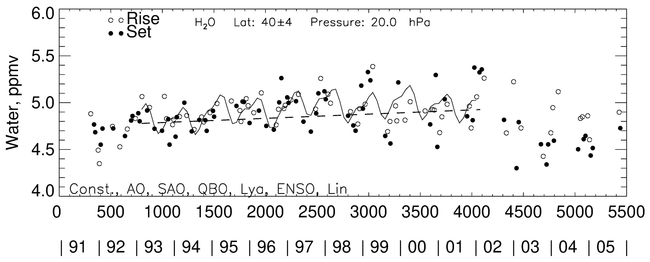
HALOE SWV trends should be most accurate in the absence of aerosols. As a check on that likelihood, Fig. 7 shows the corresponding fit of the HALOE SWV time series from 1993 to 2002 at 20 hPa or just above the top of the volcanic aerosol layer. SWV has a positive vertical mixing ratio gradient with altitude, due to the oxidation of methane to SWV in the middle stratosphere, and average SWV at 20 hPa is 4.74 ppmv or a bit higher than that at 30 hPa (4.62 ppmv). A combined AO–SAO maximum is shown clearly in Fig. 7 where the AO amplitude is twice that of the SAO, and the AO and SAO phase maxima occur on 19 February and 9 April, respectively. These seasonal cycles confirm the late-winter–early-spring moistening found in reanalysis data at 40∘ N by Konopka et al. (2022).
The HALOE SWV trend at 20 hPa for 1993–2002 is (2σ) % per decade, which agrees with that at 30 hPa from FPH ( % per decade). (There are too few FPH data at 20 hPa for a direct trend comparison with HALOE.) Yet, the HALOE trend at 20 hPa is significantly more positive than its trend at 30 hPa ( % per decade). Remsberg (2015, Table 1) reported positive trends for HALOE methane in the tropical middle stratosphere of order 10 % per decade, a small fraction (certainly less than half) of which may have undergone oxidization to SWV and subsequent transport to 40∘ N. The increase of 2.2 % per decade for the HALOE SWV trend from 30 to 20 hPa could be due to that process alone. Thus, it is inferred that the HALOE aerosol corrections at 30 hPa are small and quite reasonable over time, too.
Hegglin et al. (2014) and Remsberg (2015) showed that both methane and water vapor from limb-viewing satellite datasets (SPARC, 2017) are good indicators of seasonal variations of the BDC in the stratosphere. They reported on a hemispheric asymmetry for the net circulation, where the BDC in the Northern Hemisphere (NH) is stronger, and its methane and relative SWV trends are more positive than in the Southern Hemisphere. The strength of the NH BDC is enhanced in winter, primarily due to effects of forcings from planetary waves. There is chemical conversion of methane to water vapor in the middle and upper stratosphere followed by descent of that relatively moist air to the lower stratosphere in the region of the polar vortex.
Seasonal SWV data from the LIMS experiment illustrate the above process for 1978–1979. Figure 8 (from Remsberg et al., 2018b, their Fig. 14) displays a seasonal increase in SWV within the NH on the 550 K potential temperature surface (near 30 hPa) in terms of its area diagnostic versus equivalent latitude, which is a vortex-centered display of SWV along potential vorticity contours. Figure 8 indicates that enhanced values of water vapor descended to this surface in the vortex region by early January and continued through March. Specifically, there was an equatorward expansion of the average SWV value of 5.2 ppmv to the equivalent latitude of 40∘ N during mid-February and from mid-March onward, as the high-latitude air mixed with lower-latitude air. Note that the 550 K surface is well above the tropical tropopause, minimizing effects due to any meridional exchanges of water vapor within the lowermost stratosphere. Similar analyses of seasonal changes of ozone also show that there is further descent to lower potential temperature levels during springtime and a similar transport and mixing of polar air to lower latitudes at those levels (Curbelo et al., 2021).
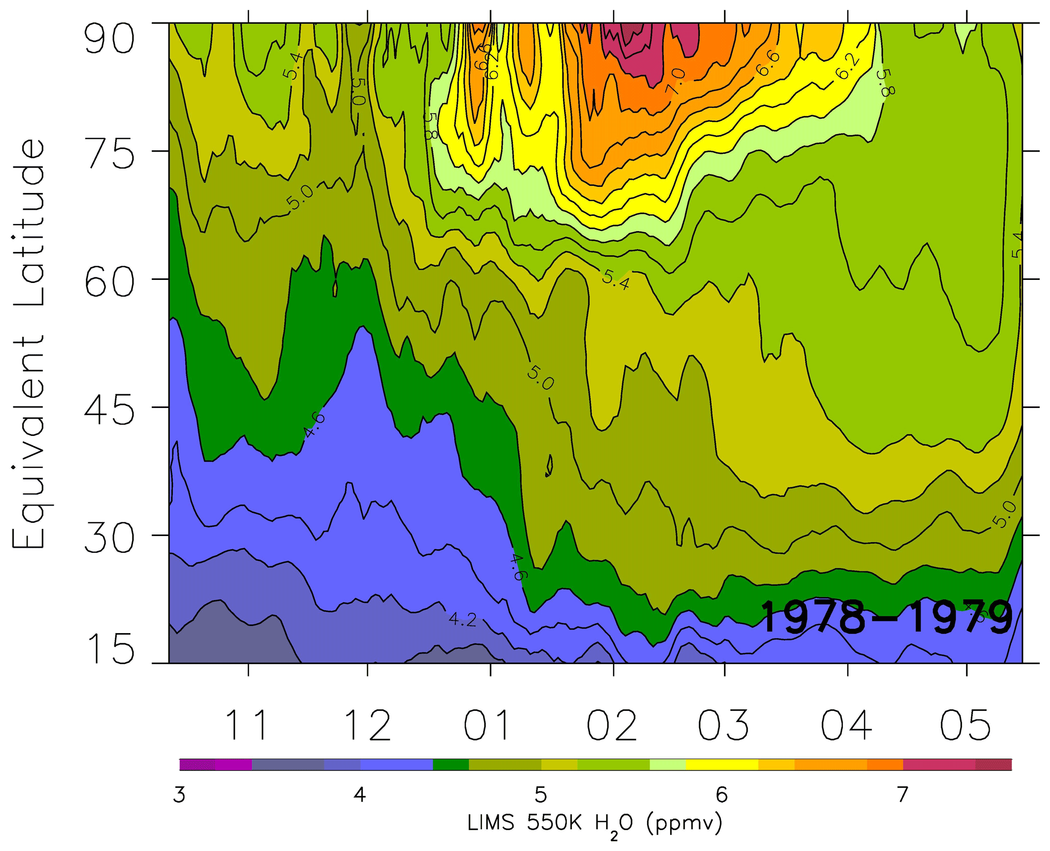
Figure 8Time series of LIMS water vapor versus equivalent latitude at 550 K and with smoothing over 7 d. Contour interval is 0.2 ppmv. Tick marks along the abscissa denote the middle of each month.
Polar plots of LIMS Version 6 (V6) geopotential height (GPH) and SWV for 17 February 1979 are in Figs. 9 and 10. They indicate the effects of meridional transport of polar air to middle latitudes, in response to a high-latitude, zonal wave-2 event. Figure 9 shows high GPH (and anticyclonic circulation) in the Aleutian and eastern Atlantic sectors and low GPH in the polar vortex (cyclonic) that extends southward across North America. The associated higher values of SWV in Fig. 10, though somewhat noisy, are characteristic of vortex air that has also undergone a southward transport. The vortex (region of highest SWV) is elongated and extends equatorward around 90 and 270∘ E. There is also a filament of high SWV (>5.5 ppmv) at the latitude of Boulder and across adjacent longitudes. The seasonal time series display of NH SWV in Fig. 8 shows that this is when the 5.2 ppmv contour extends to near 40∘ N equivalent latitude.
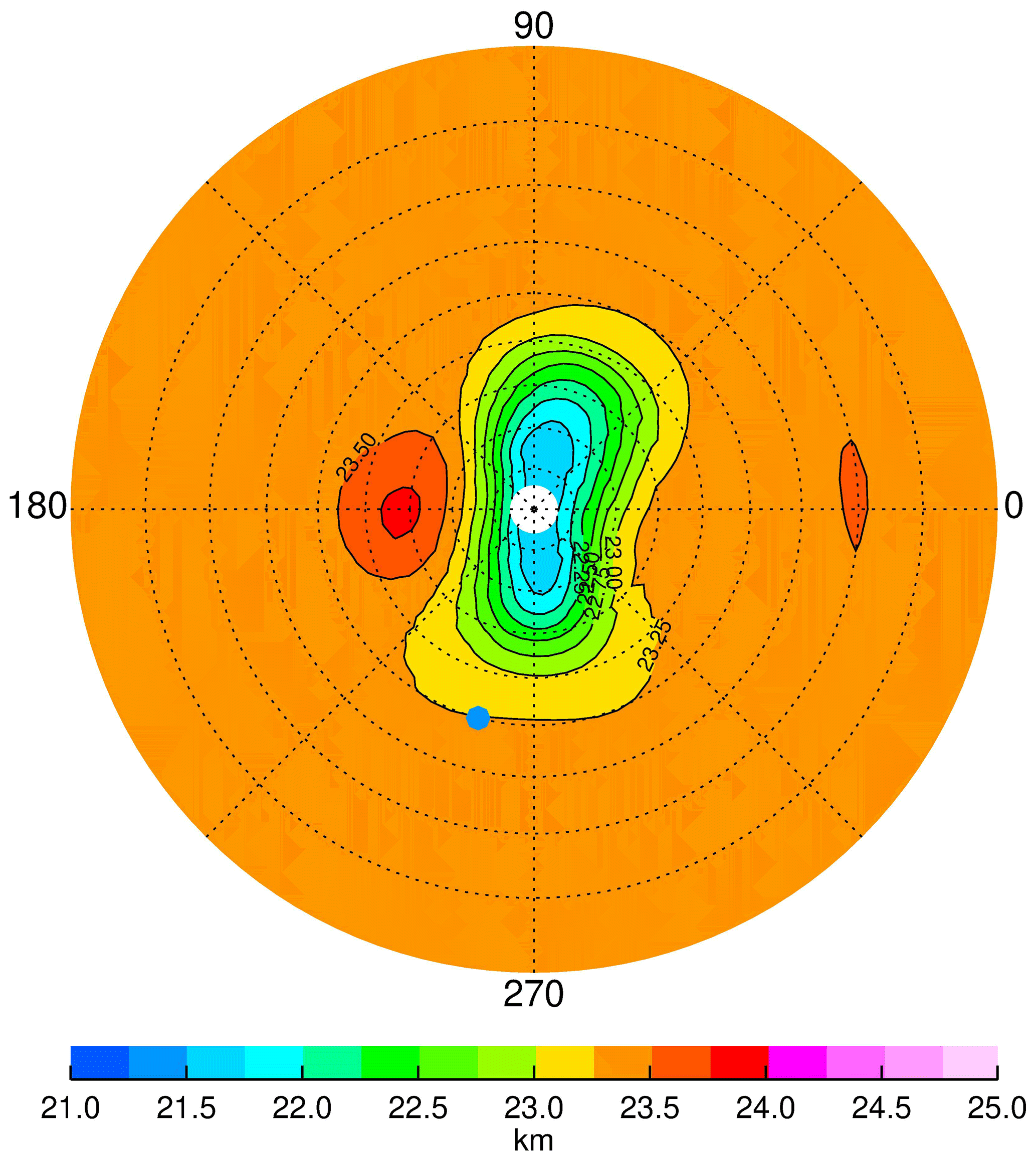
Figure 9NH plot on the 31.6 hPa surface for 17 February 1979 of LIMS geopotential height (GPH). Contour increment for GPH is 0.25 gpkm (geopotential kilometer), and dashed circles are at every 10∘ of latitude. Blue dot is location of Boulder, CO (40∘ N, 255∘ E).
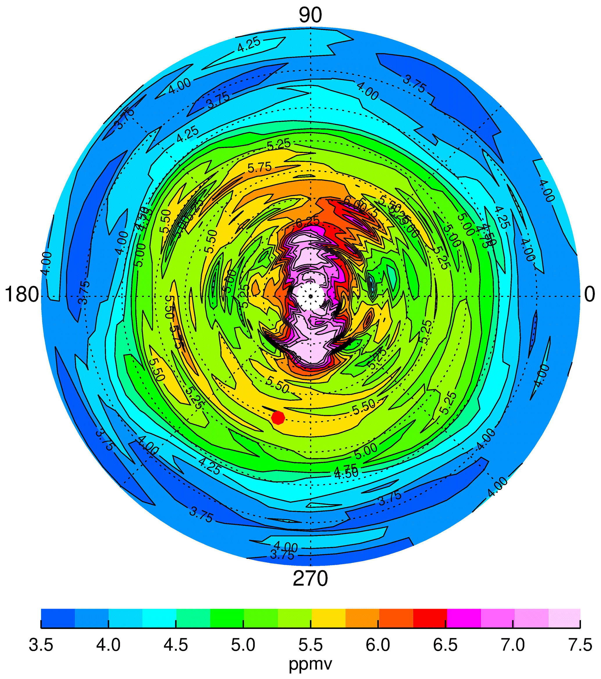
Figure 10As in Fig. 9 but for LIMS SWV on 17 February. Contour interval (CI) is 0.25 ppmv. Red dot is location of Boulder.
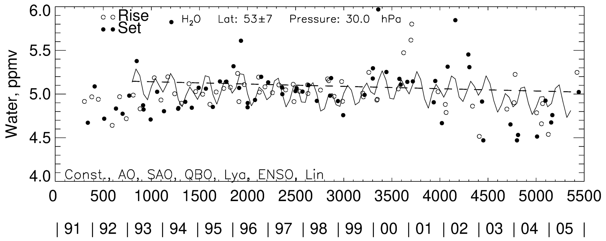
Figure 8 also indicates that there was an initial descent of polar air with higher values of SWV to near the 31.6 hPa surface around 10 January. Then there was a more general expansion of elevated SWV to the equivalent latitude of 40∘ N by the end of January (follow the 4.8 ppmv contour in Fig. 8). Similar instances of meridional transport and mixing to North American middle latitudes are a likely cause of the sporadic appearance of high SWV values during the winter and early-spring seasons of the FPH measurements in Fig. 3 and in the recent reanalysis studies of Konopka et al. (2022) and of Wargan et al. (2023). However, the HALOE time series points in Fig. 1 do not resolve such features so well because they are based on averages of four or more profiles from within the rather large sector around Boulder.
HALOE SWV time series were also analyzed for occurrences of higher SWV in three separate longitude sectors (North American, 255±35∘ E; Aleutian, 180±35∘ E; and European, 35±35∘ E) from 1993 to 2002. There are several such instances at 40∘ N in the Boulder sector (Fig. 1) but none in the Aleutian or European sectors (not shown). Conversely, Fig. 11 shows that there are several positive SWV anomalies within the higher-latitude zone of 53±7∘ N in the European sector but none in the Boulder or Aleutian sectors (not shown). SWV in Fig. 11 approaches 6.0 ppmv in four instances (on 22 April 1994, 14 April 1996, 7 March 2000, and 14–19 February 2001), and average SWV is 5.14 ppmv. All four instances are accompanied by low values of methane, which is a tracer of the transport of polar air to lower latitudes. The instances in 2000 and 2001 also occurred just after temperatures in the upper stratosphere were of order 270 K or as characteristic of a sudden stratospheric warming (SSW) event. There was a rather extended area of higher SWV over Europe, not merely a filament of vortex air, following these events.
Analyses of time series of HALOE and FPH SWV were conducted at 30 and 50 hPa for the Boulder region. Sampling frequencies for both sets of time series are of the order of a few days to several weeks. The SWV trend in the Boulder region is positive from the FPH and negative from the HALOE data from 1993 to 2005. It is assumed that the time series of FPH SWV measurements are accurate or to within their uncertainties of <6 %; the foregoing HALOE–FPH trend differences appear significant. However, there are rather large gaps at 40∘ N during late winter and spring in the HALOE time series after 2001, due to the limited power that was available for HALOE operations. This makes it is more difficult to resolve the seasonal terms and the trend term from HALOE data after 2001.
The HALOE SWV trend goes from positive to negative around 2002, and that change is a delayed effect following the sharp decrease in tropical, lower stratospheric SWV that occurred early in 2001. The FPH time series has a trend that is less positive after 2001, too, although that change is not so obvious because of the larger scatter for its points. It is more appropriate to fit two piecewise linear trends to both the HALOE and FPH time series with a break point in 2002. There are no known measurement biases that are affecting the HALOE trends. However, the retrievals of HALOE SWV do have significant and uncertain corrections for interfering aerosol extinction following the eruption of Pinatubo, particularly at 50 hPa, where the trends from HALOE and FPH disagree. The analyzed HALOE trend ( % per decade) at 30 hPa agrees more closely with that from FPH ( % per decade) or where the aerosol corrections are relatively small after 1992.
The HALOE SWV time series at 20 hPa clearly shows a springtime maximum. Northern Hemisphere SWV time series from the Limb Infrared Monitor of the Stratosphere (LIMS) experiment indicate a transport of higher SWV from polar to middle latitudes during late winter and springtime. Daily surface maps of LIMS SWV reveal filamentary structure at the latitude of 40∘ N during and following dynamically active periods. Surface maps of GPH verify that there was meridional transport of high SWV from the polar vortex to the latitude of 40∘ N at those times. Whereas FPH measurements sense SWV variations at all scales, the HALOE time series do not resolve intermediate- to smaller-scale structure because its data points are based on an average of four or more occultation profiles within a finite latitude–longitude sector centered on Boulder. It is concluded that the variations and trends of HALOE SWV are reasonably accurate at 40∘ N and 30 hPa for 1993 to 2002 and in accord with the spatial scales of its measurements and its sampling frequencies.
The LIMS V6 Level 3 product and the HALOE V19 profiles are at the NASA EARTHDATA site of EOSDIS, and their websites are https://disc.gsfc.nasa.gov/datacollection/LIMSN7L3_006.html (Remsberg et al., 2011) and https://disc.gsfc.nasa.gov/datacollection/UARHA2FN_019.html (Russell et al., 1999), respectively.
Frost-point hygrometer data from the Boulder_Lev directory were downloaded from the NOAA website at https://gml.noaa.gov/aftp/data/ozwv/WaterVapor/Boulder_New/ (Hurst, 2016).
The author has declared that there are no competing interests.
Publisher's note: Copernicus Publications remains neutral with regard to jurisdictional claims in published maps and institutional affiliations.
This article is part of the special issue “Water vapour in the upper troposphere and middle atmosphere: a WCRP/SPARC satellite data quality assessment including biases, variability, and drifts (ACP/AMT/ESSD inter-journal SI)”. It is not associated with a conference.
Ellis Remsberg thanks V. Lynn Harvey for generating the plot in Fig. 8 that appeared originally in Remsberg et al. (2018b). Ellis Remsberg also appreciates comments by Mark Hervig on a draft of the manuscript. Ellis Remsberg carried out this work while serving as a Distinguished Research Associate of the Science Directorate at NASA Langley.
This paper was edited by Aurélien Podglajen and reviewed by two anonymous referees.
Bhatt, P. P., Remsberg, E. E., Gordley, L. L., McInerney, J. M., Brackett, V. G., and Russell IlI, J. M.: An evaluation of the quality of Halogen Occultation Experiment ozone profiles in the lower stratosphere, J. Geophys. Res., 104, 9261–9275, https://doi.org/10.1029/1999JD900058, 1999.
Charlton, A. J. and Polvani, L. M.: A New Look at Stratospheric Sudden Warmings. Part I: Climatology and Modeling Benchmarks, J. Climate, 20, 449–469, https://doi.org/10.1175/JCLI3996.1, 2007.
Curbelo, J., Chen, G., and Mechoso, C. R.: Lagrangian analysis of the northern stratospheric polar vortex split in April 2020. Geophys. Res. Lett., 48, e2021GL093874, https://doi.org/10.1029/2021GL093874, 2021.
Davis, S. M., Rosenlof, K. H., Hassler, B., Hurst, D. F., Read, W. G., Vömel, H., Selkirk, H., Fujiwara, M., and Damadeo, R.: The stratospheric water and ozone satellite homogenized (SWOOSH) database: a long-term database for climate studies, Earth Syst. Sci. Data, 8, 461–490, https://doi.org/10.5194/essd-8-461-2016, 2016.
Gordley, L. L., Thompson, E., McHugh, M., Remsberg, E., Russell III, J., and Magill, B.: Accuracy of atmospheric trends inferred from the Halogen Occultation Experiment data, J. Appl. Remote Sens., 3, 033526, https://doi.org/10.1117/1.3131722, 2009.
Hall, E. G., Jordan, A. F., Hurst, D. F., Oltmans, S. J., Vömel, H., Kühnreich, B., and Ebert, V.: Advancements, measurement uncertainties, and recent comparisons of the NOAA frost point hygrometer, Atmos. Meas. Tech., 9, 4295–4310, https://doi.org/10.5194/amt-9-4295-2016, 2016.
Harries, J. E., Russell III, J. M., Tuck, A. F., Gordley, L. L., Purcell, P., Stone, K., Bevilacqua, R. M., Gunson, M., Nedoluha, G., and Traub, W. A.: Validation of measurements of water vapor from the Halogen Occultation Experiment (HALOE), J. Geophys. Res., 101, 10205–10216, https://doi.org/10.1029/95JD02933, 1996.
Hegglin, M. I., Plummer, D. A., Shepherd, T. G., Scinocca, J. F., Anderson, J., Froidevaux, L., Funke, B., Hurst, D., Rozanov, A., Urban, J., von Clarmann, T., Walker, K. A., Wang, H. J., Tegtmeier, S., and Weigel, K.: Vertical structure of stratospheric water vapour trends derived from merged satellite data, Nat. Geosci., 7, 768–776, https://doi.org/10.1038/NGEO2236, 2014.
Hervig, M. E., Russell III, J. M., Gordley, L. L., Daniels, J., Drayson, S. R., and Park, J. H.: Aerosol effects and corrections in the Halogen Occultation Experiment, J. Geophys. Res., 100, 1067–1079, https://doi.org/10.1029/94JD02143, 1995.
Hervig, M. E., Russell III, J. M., Gordley, L. L., Park, J. H., Drayson, S. R., and Deshler, T.: Validation of aerosol measurements from the Halogen Occultation Experiment, J. Geophys. Res., 101, 10267–10275, https://doi.org/10.1029/95JD02464, 1996.
Hurst, D.: Water Vapor and Ozone Vertical Profile Data, Boulder, CO, USA, Ozone and Water Vapor Research Group, Earth System Research Laboratory, ESRL/GMD/OZWVNOAA/ESRL/Global Monitoring Division, NOAA, U.S. Dept. of Commerce [data set], https://gml.noaa.gov/aftp/data/ozwv/WaterVapor/Boulder_New/ (last access: 23 August 2023), 2016.
Hurst, D. F., Oltmans, S. J., Vömel, H., Rosenlof, K. H., Davis, S. M., Ray, E. A., Hall, E. G., and Jordan, A. F.: Stratospheric water vapor trends over Boulder, Colorado: Analysis of the 30 year Boulder record, J. Geophys. Res., 116, 148–227, https://doi.org/10.1029/2010JD015065, 2011.
Konopka, P., Tao, M., Ploeger, F., Hurst, D. F., Santee, M. L., Wright, J. S., and Riese, M.: Stratospheric moistening after 2000, Geophys. Res. Lett., 49, e2021GL097609, https://doi.org/10.1029/2021GL097609, 2022.
Lossow, S., Hurst, D. F., Rosenlof, K. H., Stiller, G. P., von Clarmann, T., Brinkop, S., Dameris, M., Jöckel, P., Kinnison, D. E., Plieninger, J., Plummer, D. A., Ploeger, F., Read, W. G., Remsberg, E. E., Russell III, J. M., and Tao, M.: Trend differences in lower stratospheric water vapour between Boulder and the zonal mean and their role in understanding fundamental observational discrepancies, Atmos. Chem. Phys., 18, 8331–8351, https://doi.org/10.5194/acp-18-8331-2018, 2018.
Manney, G. L., Millan, L. F., Santee, M. L., Wargan, K., Lambert, A., Neu, J. L., Werner, F., Lawrence, Z. D., Schwartz, M. J., Livesey, N. J., and Read, W. G.: Signatures of Anomalous Transport in the 2019/2020 Arctic Stratospheric Polar Vortex, J. Geophys. Res.-Atmos., 127, e2022JD037407, https://doi.org/10.1029/2022JD037407, 2022.
Randel, W. J., Wu, F., Vömel, H., Nedoluha, G. E., and Forster, P.: Decreases in stratospheric water vapor after 2001: Links to changes in the tropical tropopause and the Brewer-Dobson circulation, J. Geophys. Res.-Atmos., 111, D12312, https://doi.org/10.1029/2005JD006744, 2006.
Remsberg, E.: Methane as a diagnostic tracer of changes in the Brewer-Dobson circulation of the stratosphere, Atmos. Chem. Phys., 15, 3739–3754, https://doi.org/10.5194/acp-15-3739-2015, 2015.
Remsberg, E., Damadeo, R., Natarajan, M., and Bhatt, P.: Observed responses of mesospheric water vapor to solar cycle and dynamical forcings, J. Geophys. Res., 123, 3830–3843, https://doi.org/10.1002/2017JD028029, 2018a.
Remsberg, E., Natarajan, M., and Harvey, V. L.: On the consistency of HNO3 and NO2 in the Aleutian High region from the Nimbus 7 LIMS Version 6 dataset, Atmos. Meas. Tech., 11, 3611–3626, https://doi.org/10.5194/amt-11-3611-2018, 2018b.
Remsberg, E., Lingenfelser, G., and Natarajan, M.: LIMS/Nimbus-7 Level 3 Daily 2 deg Latitude Zonal Fourier Coefficients of O3, NO2, H2O, HNO3, Geopotential Height, and Temperature V006, Greenbelt, MD, USA, Goddard Earth Sciences Data and Information Services Center (GES DISC) [data set], https://disc.gsfc.nasa.gov/datacollection/LIMSN7L3_006.html (last access: 23 August 2023), 2011.
Remsberg, E. E.: On the response of Halogen Occultation Experiment (HALOE) stratospheric ozone and temperature to the 11-yr solar cycle forcing, J. Geophys. Res.-Atmos., 113, D02304, https://doi.org/10.1029/2008JD010189, 2008.
Russell III, J. M., et al.: UARS Halogen Occultation Experiment (HALOE) Level 2 V019, Greenbelt, MD, USA, Goddard Earth Sciences Data and Information Services Center (GES DISC) [data set], https://disc.gsfc.nasa.gov/datacollection/UARHA2FN_019.html (last access: 23 August 2023), 1999.
Scherer, M., Vömel, H., Fueglistaler, S., Oltmans, S. J., and Staehelin, J.: Trends and variability of midlatitude stratospheric water vapour deduced from the re-evaluated Boulder balloon series and HALOE, Atmos. Chem. Phys., 8, 1391–1402, https://doi.org/10.5194/acp-8-1391-2008, 2008.
SPARC: Report No. 8 of the SPARC Data Initiative, Assessment of stratospheric trace gas and aerosol climatologies from satellite limb sounders, Prepared by the SPARC Data Initiative Team, edited by: Hegglin, M. I. and Tegtmeier, S., WCRP-5/2017, ETH Zürich, Geneva, https://doi.org/10.3929/ethz-a-010863911, 2017.
Tiao, G. C., Reinsel, G. C., Xu, D., Pedrick, J. H., Zhu, X., Miller, A. J., DeLuisi, J. J., Mateer, C. L., and Wuebbles, D. J.: Effects of autocorrelation and temporal sampling schemes on estimates of trend and spatial correlation, J. Geophys. Res., 95, 20507–20517, https://doi.org/10.1029/JD095iD12p20507, 1990.
Wargan, K., Weir, B., Manney, G. L., Cohn, S. E., Knowland, K. E., Wales, P. A., and Livesey, N. J.: M2-SCREAM: A stratospheric composition reanalysis of Aura MLS data with MERRA-2 transport, Earth Space Sci., 10, e2022EA002632, https://doi.org/10.1029/2022EA002632, 2023.
- Abstract
- Background and objective
- Time series analyses of HALOE SWV near Boulder
- Time series of FPH measurements of SWV
- Uncertainties for the HALOE SWV trends
- Source for the springtime moistening at 40∘ N
- Summary and conclusions
- Data availability
- Competing interests
- Disclaimer
- Special issue statement
- Acknowledgements
- Review statement
- References