High-resolution air quality simulations of ozone exceedance events during the Lake Michigan Ozone Study

We evaluate two high-resolution Lake Michigan air quality simulations during the 2017 Lake Michigan Ozone Study campaign. These air quality simulations employ identical chemical configurations but use different input meteorology. The AP-XM configuration follows the U.S. Environmental Protection Agency (EPA)-recommended modeling practices, whereas the YNT_SSNG employs different parameterization schemes and satellite-based inputs of sea surface temperatures, green vegetative fraction, and soil moisture and temperature. Overall, we find a similar performance in the model simulations of hourly and maximum daily average 8 h (MDA8) ozone, with the AP-XM and YNT_SSNG simulations showing biases of −11.42 and −13.54 ppbv (parts per billion by volume), respectively, during periods when the observed MDA8 was greater than 70 ppbv. However, for the two monitoring sites that observed high-ozone events, the AP-XM simulation better matched observations at Chiwaukee Prairie, and the YNT_SSNG simulation better matched observations at the Sheboygan Kohler-Andrae (KA) State Park. We find that the differences between the two simulations are largest for column amounts of ozone precursors, particularly NO₂. Across three high-ozone events, the YNT_SSNG simulation has a lower NO₂ column bias (0.17×10¹⁵ mol cm⁻²) compared to the AP-XM simulation (0.31×10¹⁵ mol cm⁻²). The YNT_SSNG simulation also has an advantage in that it better captures the structure of the boundary layer and lake breeze during the 2 June high-ozone event, although the timing of the lake breeze is about 3 h too early at Sheboygan. Our results are useful for informing an air quality modeling framework for the Lake Michigan area.

1 Introduction

Ground-level ozone has many well-documented effects on human health, including increased risk for respiratory and cardiovascular diseases and even premature death (Di et al., 2017; Lelieveld et al., 2015; Manisalidis et al., 2020). Ozone also damages plant tissue by affecting crop health (e.g., Clifton et al., 2020; Shindell et al., 2012). Ground-level ozone is formed by photochemical reactions between nitrogen oxides (NO_x) and volatile organic compounds (VOCs); major NO_x sources include fuel combustion, biomass burning, soil microbes, and lightning, with anthropogenic sources being dominant (Hall et al., 1996; Juncosa Calahorrano et al., 2020; Lamsal et al., 2010; Lawrence and Crutzen, 1999; Nault et al., 2017). Major sources of VOCs include industrial processes and natural sources, such as trees (Guenther et al., 1995; He et al., 2019).

The areas along the Lake Michigan shoreline are susceptible to high-ozone amounts because of a combination of abundant precursor emissions and transport processes, particularly the lake breeze circulation. The relationships between area emissions and meteorology as they impact air quality along the Lake Michigan shoreline have been characterized in field campaigns (Sexton and Westberg, 1980; Dye et al., 1995; Foley et al., 2011; Stanier et al., 2021), and the meteorological component is the subject of Part 1 of this study (Otkin et al., 2023). Ozone concentrations along coastlines can be enhanced significantly when urban emissions react within the shallow, stable marine boundary layer (Fast and Heilman, 2003). The lake breeze circulation is particularly important for enhanced ozone production over Lake Michigan, where it contributes to roughly 80 % of high-ozone episodes observed in eastern Wisconsin (Lennartson and Schwartz, 2002; Cleary et al., 2021). Lake breeze circulations impact ozone concentrations elsewhere in the Great Lakes, including southern Ontario (Makar et al., 2010; He et al., 2011; Brook et al., 2013; Stroud et al., 2020).

As highlighted by Dye et al. (1995), there has been a need for a modeling framework that represents the finer scales of emissions transport and chemistry near the Lake Michigan shoreline. It is our opinion that developing emission control strategies to mitigate these coastal high-ozone events requires accurate prediction of the lake breeze transport processes at scales of 1–10 km. Furthermore, these chemical transport processes cannot be accurately resolved using the 12 km resolution meteorological and chemical simulations typically used in air quality modeling for previous SIPs.

We have developed a high-resolution, satellite-constrained meteorological modeling platform for the United States Midwest that supports the needs of the Lake Michigan Air Directors Consortium (LADCO), as they conduct detailed air quality modeling assessments for its member states. In Part I of this study, Otkin et al. (2023) assessed the impact of different high-resolution surface datasets, parameterization schemes, and analysis nudging on near-surface meteorological conditions and energy fluxes relative to the model configuration and input datasets typically employed by the U.S. Environmental Protection Agency (EPA). In Part II of this study, we use the meteorological output obtained from two of these simulations as input to the EPA Community Multiscale Air Quality (CMAQ), model version 5.2.1 (Byun and Schere, 2006; Nolte et al., 2015), model simulations to assess the impact of these model changes on ozone forecasts in the Lake Michigan region. The remainder of this paper is organized as follows: Sect. 2 contains a description of the CMAQ model configurations and observational data used for evaluation. The results are presented in Sect. 3, with the discussion and conclusions provided in Sect. 4.

2 Methods

In this work, we compare two CMAQ simulations, one with baseline meteorology and the other with meteorology from our optimized Weather Research and Forecasting (WRF) model configuration, as detailed in Part I (Otkin et al., 2023). Both sets of meteorological simulations employ a triple-nested domain configuration containing 12, 4, and 1.33333 (1.3) km resolution grids, respectively (Fig. 1 in Otkin et al., 2023), constrained to 6 h, 0.25^∘ resolution Global Forecast System Final (GFS-FNL) analyses and using the rapid radiative transfer model for general circulation models (RRTMG) longwave and shortwave radiation (Iacono et al., 2008; Mlawer et al., 1997) on all three domains, along with the Kain–Fritsch cumulus scheme (Kain, 2004) on the outer two domains and an explicit convection on the innermost domain. Both simulations have the same vertical resolution throughout, with six model layers below 200 m, four model layers below 100 m, and the lowest three layers at ∼9, 27, and 55 m a.g.l. (above ground level). The AP-XM simulation employs the Morrison microphysics (Morrison et al., 2005), ACM2 planetary boundary layer (PBL; Pleim, 2007), and the Pleim–Xu LSM (Gilliam and Pleim, 2010; Xiu and Pleim, 2001) parameterization schemes, which are the same schemes used within CMAQ and are therefore considered our baseline meteorological simulation. Our optimized meteorological modeling platform uses the Yonsei University (YSU) PBL (Hong et al., 2006), Noah LSM (Chen and Dudhia, 2001; Ek et al., 2003), and Thompson microphysics (Thompson et al., 2008, 2016) schemes, which are constrained by high-resolution (1 km) soil moisture and temperature analyses (Case, 2016; Case and Zavodsky, 2018; Blankenship et al., 2018) from the Short-term Prediction Research and Transition Center (SPoRT), daily high-resolution (1.3 km) Great Lakes surface temperatures (Schwab, 1992) from the Great Lakes Surface Environmental Analysis (GLSEA), and high-resolution (4 km) green vegetation fraction (GVF) from the Visible Infrared Imaging Radiometer Suite (VIIRS; Vargas et al., 2015) instead of the monthly GVF climatologies. This optimized configuration is hereafter referred to as the YNT_SSNG. Otkin et al. (2023) found that the AP-XM configuration generally produced more accurate meteorological analyses on the 12 km domain, but its accuracy decreased with a finer model grid resolution. In contrast, the YNT_SSNG statistics showed consistent reductions in the root mean square error (RMSE) for 2 m temperature, 2 m water vapor mixing ratio, and 10 m wind speed relative to the AP-XM as the model resolution increased from 12 to 1.3 km. We note that differences in near-surface wind speed and GVF will also impact the deposition velocities in the CMAQ simulations.

Each CMAQ simulation is run with the same configuration and anthropogenic emissions. Using CMAQv5.2.1 (Appel et al., 2017; US EPA, 2018), our configuration includes AERO6 aerosol chemistry, the Carbon Bond 6 chemical mechanism, revision 3 (CB6r3; Emery et al., 2015; Luecken et al., 2019), and in-line photolysis. CMAQ was run with 39 vertical layers, with a top layer of approximately 100 hPa, thus using all available layers from our WRF simulations. As with our WRF simulations, we ran CMAQ on three domains, namely one using a 12 km by 12 km horizontal resolution over the continental USA (396×246 grid points), one using a 4 km by 4 km horizontal resolution over the upper Midwest (447×423 grid points), and one using a 1.3 km by 1.3 km horizontal resolution over Lake Michigan and the nearby areas (245×506 grid points). The 12 km CMAQ simulations employ lateral boundary conditions (LBCs) from the global Real-time Air Quality Modeling System (RAQMS) model (Pierce et al., 2007), which includes the assimilation of ozone retrievals from the Microwave Limb Sounder (MLS) and Ozone Monitoring Instrument (OMI) on the NASA Aura satellite and the assimilation of aerosol optical depth (AOD) from the Moderate Resolution Imaging Spectroradiometer (MODIS) on the NASA Terra and Aqua satellites. Utilizing RAQMS LBCs for CMAQ continental-scale simulations has been shown to significantly increase upper tropospheric ozone, to improve the daily maximum surface O₃ concentrations (Song et al., 2008), and to improve the agreement with OMI tropospheric ozone column (Lee et al., 2012) relative to fixed LBCs. The 4 and 1.3 km simulations employ lateral boundary conditions from the respective parent grid.

Anthropogenic emissions for the 12 km domain were taken from the 2016 National Emissions Inventory Collaborative (NEIC, 2019), version 1. Anthropogenic emissions for the 4 and 1.3 km domains were taken from the 2017 National Emissions Inventory, version 1 (US EPA, 2021; Adams, 2020), where emissions on the 4 km domain were provided by the EPA (Kirk Baker, personal communication, 2020), and then interpolated and downscaled by one-ninth for use on the 1.3 km domain. We acknowledge that the use of downscaled 4 km emissions will degrade the performance of the 1.3 km simulations, but generating 1.3 km area emissions from the Sparse Matrix Operator Kernel Emissions (SMOKE) programs was beyond the scope of this project. Biogenic emissions were calculated in-line, using the Biogenic Emission Inventory System (BEIS) with the Biogenic Emissions Landuse Database, Version 3 (BELD3; Carlton and Baker, 2011). Meteorologically sensitive input for biogenic emissions calculations (such as frost dates) was generated separately for each set of CMAQ simulations using SMOKE programs. As biogenic emissions are calculated in-line, they vary among our configurations with differing input meteorology and GVF.

We focus on the innermost 1.3 km domain surrounding Lake Michigan during the 2017 Lake Michigan Ozone Study (LMOS) field campaign (Stanier et al., 2021) which occurred from 22 May–22 June 2017. Our chemical evaluation focuses on ozone and three of its precursors, nitrogen dioxide, formaldehyde and isoprene, in the surface layer and in the atmospheric column. We employ ozone observations from the Air Quality System (AQS) monitoring network, using the Atmospheric Model Evaluation Tool (AMET) developed by the EPA. We also utilize nitrogen dioxide (NO₂) and formaldehyde (HCHO) in situ observations from an EPA trailer that was deployed at Sheboygan, WI, and NO₂ and isoprene measurements from the LMOS Zion, IL, supersite (Stanier et al., 2021). In situ O₃ and wind observations at select monitors were submitted to the LMOS data repository (https://asdc.larc.nasa.gov/soot/power-user/LMOS/2017, last access: 27 August 2023). For column evaluation, we employ observations of NO₂ and HCHO columns from the Geostationary Trace gas and Aerosol Sensor Optimization (GeoTASO; Leitch et al., 2014) instrument taken during LMOS (Judd et al., 2019).

3 Results

We first evaluate the model performance of the AP-XM and YNT_SSNG simulations over the entire LMOS period, based on the ozone precursors of NO₂, HCHO, and isoprene, as well as daily 8 h maximum ozone. Used in the NAAQS for ozone, maximum 8 h ozone amounts are calculated as a rolling 8 h average for each day, starting for the period of 07:00 to 15:00 local standard time (LST) and ending with the period of 23:00 to 07:00 LST on the following day. However, 8 h maximum ozone is strongly influenced by days with low- and moderate-ozone concentrations. Though only 5.9 % (112) of the 8 h maximum ozone periods within the 1.3 km domain were above the NAAQS threshold for ozone (70 ppbv – parts per billion by volume) during LMOS (see Fig. 1), it is these higher 8 h maximum ozone values that are most relevant to SIP modeling.

To evaluate the simulations more precisely, we then evaluate the high-ozone days as identified by the two coastal AQS monitors that tend to show the highest-ozone concentrations. High-ozone days with extensive observations during LMOS 2017 include 2–4, 9–12, and 14–16 June (Abdi-Oskouei et al., 2020) and are referred to as events A, B, and C, respectively. Finally, we evaluate model performance over the broader western Lake Michigan shoreline area during the only ozone exceedance event on 2 June.

3.1 Model performance over the entire LMOS period

3.1.1 The 8 h maximum ozone

Figure 1 shows binned whisker plots of 8 h maximum ozone bias and RMSE at 10 ppb (parts per billion) intervals for the 1.3 km simulations for all sites within the 1.3 km domain. Systematic high biases for lower-ozone concentrations (≲40 ppbv) and a low bias for higher-ozone concentrations (>50 ppbv) are evident in both simulations. The YNT_SSNG and AP-XM simulations show similar biases and RMSE for 8 h maximum ozone concentrations between 40–80 ppbv, but the AP-XM shows significantly lower biases and RMSE in the 80–90 ppbv bin. Figure 2 shows the geographical distribution of 8 h maximum ozone bias and RMSE for the 1.3 km AP-XM and YNT_SSNG for all AQS sites within the 1.3 km domain. Overall biases are largely negative, reflecting underestimates of 8 h maximum ozone at the AQS sites. When compared on a site-by-site basis, the biases and RMSE in 8 h maximum ozone are generally smaller by more than 2 ppbv in the YNT_SSNG simulation, with the exception of two AQS sites in northern Chicago where the YNT_SSNG simulations show overestimates of 4–8 ppbv in 8 h maximum ozone. This may be due to the use of a more realistic and lower (relative to climatology) green vegetation fraction (see Fig. 2 in Otkin et al., 2023) in the YNT_SSNG simulation, which would tend to reduce ozone deposition velocities and increase ozone concentrations (Ran et al., 2016).

Figure 1 Whisker plots showing the bias (a) and RMSE (b) for binned 8 h maximum ozone concentrations from the AP-XM (gray) and YNT_SSNG (red) CMAQ simulations using hourly data within the 1.3 km resolution domain during the LMOS period of record from 22 May 2017 to 22 June 2017. Triangles and circles represent the conditional distribution medians, stars represent distribution means, and lines and whiskers represent the lower quartile and upper quartile ranges.

Figure 2 Geographical distribution of bias (a, b) and RMSE (c, d) for binned 8 h maximum ozone concentrations from the AP-XM (a, c) and YNT_SSNG (b, d) 1.3 km CMAQ simulations, using hourly data from all stations in the 1.3 km resolution inner domain during the LMOS period of record from 22 May 2017 to 22 June 2017. Bias and RMSE (ppbv) at each site are indicated by the color bar. Two AQS monitors, at the Sheboygan Kohler-Andrae (KA) State Park to the north and Chiwaukee Prairie along the Wisconsin–Illinois border, are indicated by the red circles.

3.1.2 Evaluation with Sheboygan, WI, ground-based NO₂ and HCHO measurements

During LMOS, the EPA deployed instruments measuring in situ NO₂ and HCHO in Sheboygan, WI, to characterize ozone precursors along the shore of Lake Michigan. These 1 min measurements were taken at Spaceport Sheboygan, which is approximately 9 km north of the Sheboygan Kohler-Andrae (KA) State Park monitor (highlighted in Fig. 2). Here, we use the hourly averaged EPA NO₂ and HCHO measurements to evaluate the accuracy of the prediction of ozone precursors at Sheboygan for the YNT_SSNG and AP-XM CMAQ simulations.

Figures 3 and 4 show the hourly NO₂ and HCHO comparisons, respectively. There are several periods in which the observed NO₂ (black lines; Fig. 3) is above 10 ppbv; these periods are generally underestimated by the AP-XM simulation and overestimated by the YNT_SSNG simulation (red lines; Fig. 3). We find an overall slightly positive bias of 0.19 ppbv for the AP-XM and an overall positive bias of 0.68 ppbv for the YNT_SSNG simulation. We also find that the correlations are slightly lower and RMSEs are slightly higher in the YNT_SSNG simulation than in the AP-XM simulation.

Observed HCHO shows peak amounts in excess of 4 ppbv (black lines; Fig. 4), which are underestimated in both simulations (red lines; Fig. 4). However, the YNT_SSNG simulation tends to have overall higher HCHO mixing ratios than the AP-XM simulation, leading to a reduction (−0.26 versus −0.43 ppbv) in the low bias relative to the EPA measurements. This is despite the fact that the YNT_SSNG uses a more realistic and lower (relative to climatology) green vegetation fraction (see Fig. 2 in Otkin et al., 2023), which would tend to reduce biogenic VOC emissions. This suggests that anthropogenic VOC emissions may be playing a role in the reduction in the low biases in the YNT_SSNG simulation. Compared to the AP-XM simulation, we also find correlations, and the RMSEs are slightly lower in the YNT_SSNG simulation.

The larger high biases in NO₂ and reduced low biases in HCHO in the YNT_SSNG simulation lead to significant reductions in the high biases in ozone in the YNT_SSNG compared to the AP-XM simulation (0.07 versus 1.76 ppbv; not shown) and may be due to more nighttime ozone titration in the YNT_SSNG simulation.

Figure 3 Time series of 1 h averaged NO₂ at Spaceport Sheboygan for the 1.3 km AP-XM (a) and YNT_SSNG (b) CMAQ simulations (red) and EPA observations (black) during the LMOS 2017 time period (22 May–21 June 2017).

Figure 4 Time series of 1 h averaged HCHO at Spaceport Sheboygan for the 1.3 km AP-XM (a) and YNT_SSNG (b) CMAQ simulations (red) and EPA observations (black) during the LMOS 2017 time period (22 May–21 June 2017).

3.1.3 Evaluation with Zion, IL, ground-based NO₂ and isoprene measurements

During LMOS, the University of Wisconsin–Madison deployed a Thermo Scientific Model 42i NO–NO₂–NO₂ analyzer instrument to measure in situ NO₂, and the University of Minnesota deployed a proton transfer reaction quadrupole interface time-of-flight mass spectrometer (PTR-QiTOF-MS) to measure isoprene at the LMOS Zion, IL, ground site to characterize ozone precursors along the shore of Lake Michigan. These 1 min measurements were co-located at the Illinois Ambient Air Monitoring site (17-097-1007) in Illinois Beach State Park, which is approximately 4 km south of the Chiwaukee monitor highlighted in Fig. 2. Here, we use the hourly averaged NO₂ and isoprene measurements to evaluate the accuracy of prediction of ozone precursors at Zion, IL, for the YNT_SSNG and AP-XM CMAQ simulations.

Figures 5 and 6 show the hourly NO₂ and isoprene comparisons, respectively. There are several periods in which observed NO₂ (black lines; Fig. 5) is above 10 ppbv; these periods are generally overestimated by the AP-XM simulation, with the YNT_SSNG simulation being in much better agreement with the observations (red lines; Fig. 5). We find an overall positive bias of 1.86 ppbv for the AP-XM and an overall positive bias of 1.39 ppbv for the YNT_SSNG simulation. We also find that the correlations are slightly lower, and the RMSEs are lower in the YNT_SSNG simulation than in the AP-XM simulation.

Observed isoprene shows peak amounts in excess of 4 ppbv (black lines; Fig. 6) which are significantly underestimated in both simulations (red lines; Fig. 6). The YNT_SSNG simulation tends to have overall lower isoprene mixing ratios than the AP-XM simulation, leading to a larger low bias (−0.34 versus −0.28 ppbv) for the YNT_SSNG simulation relative to the Zion, IL, measurements. This is consistent with the use of more realistic and lower (relative to climatology) green vegetation fraction in the YNT_SSNG simulation (see Fig. 2 in Otkin et al., 2023). We also find that correlations with observed isoprene are higher and RMSEs are slightly higher in the YNT_SSNG simulation.

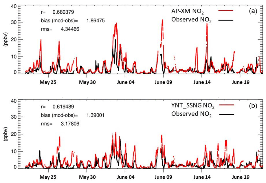
Figure 5 Time series of 1 h averaged NO₂ at Zion, IL, for the 1.3 km AP-XM (a) and YNT_SSNG (b) CMAQ simulations (red) and observations (black) during the LMOS 2017 time period (21 May–22 June 2017).

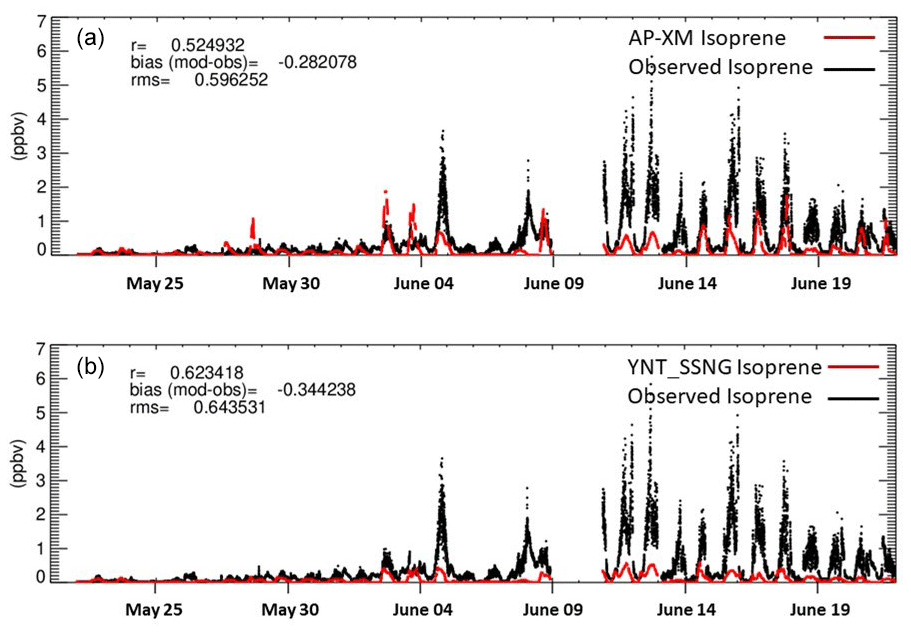
Figure 6 Time series of 1 h averaged isoprene at Zion, IL, for the 1.3 km AP-XM (a) and YNT_SSNG (b) CMAQ simulations (red) and observations (black) during the LMOS 2017 time period (21 May–22 June 2017).

3.2 Model performance during high-ozone events

3.2.1 Sheboygan KA and Chiwaukee Prairie 1 h ozone

In this and the following sections, we focus on the following two AQS monitors that showed high-ozone events during LMOS most clearly: the Sheboygan Kohler-Andrae (KA) State Park monitor (AQS 551170006), located south of Sheboygan, WI, and the Chiwaukee Prairie monitor (AQS 550590019), which is located near the Wisconsin–Illinois border. These two sites are indicated by red circles in Fig. 2.

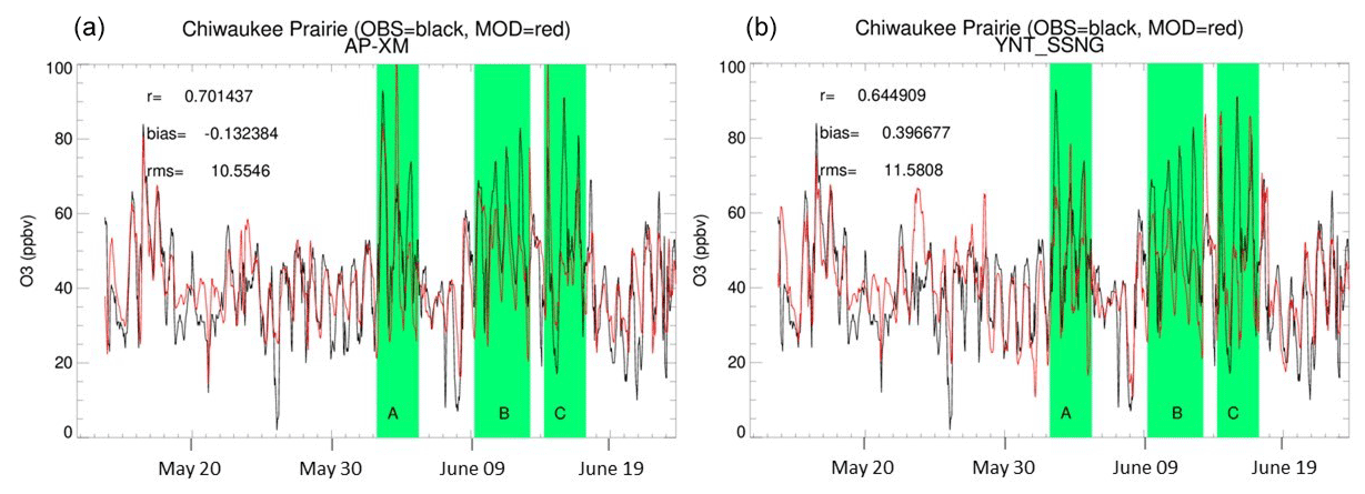
Figures 7 and 8 show the hourly AQS observed and CMAQ AP-XM and YNT_SSNG simulated O₃ for Sheboygan KA and Chiwaukee Prairie monitors. Comparisons with AQS observations and the two simulations at Sheboygan KA show similar correlations (0.74 versus 0.73), reduced biases (1.01 versus −1.9 ppbv), and similar RMSE (9.97 versus 10.3 ppbv) for the YNT_SSNG relative to the AP-XM simulation. Similar comparisons at Chiwaukee Prairie show decreased correlations (0.64 versus 0.70), higher biases (0.4 versus −0.13 ppbv), and increased RMSE (11.58 versus 11.58 ppbv) for the YNT_SSNG relative to the AP-XM simulation. Student t tests between the AP-XM and YNT_SSNG simulations at each site show that the simulations have statistically significant differences (99 % confidence level) in the mean ozone concentration at Sheboygan KA but not at Chiwaukee Prairie. While the overall hourly ozone statistics at Sheboygan KA and Chiwaukee Prairie are relatively similar between the AP-XM and YNT_SSNG simulations at these sites, the simulations during high-ozone events are quite different. This is illustrated by looking at composite statistics during events A, B, and C.

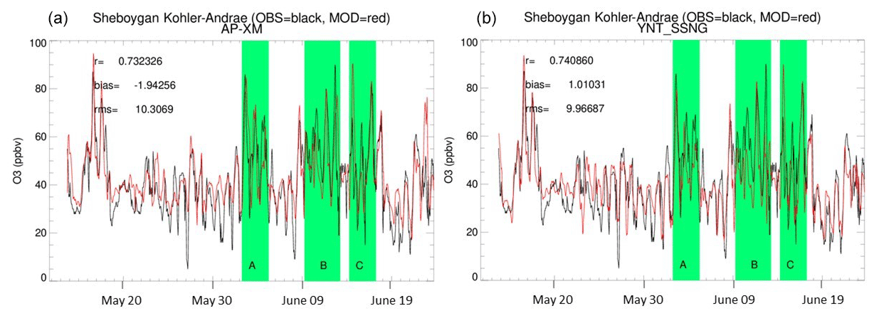
Figure 7 Time series of 1 h ozone at Sheboygan Kohler-Andrae (KA) AQS monitor (551170006) for the 1.3 km AP-XM (a) and YNT_SSNG (b) CMAQ simulations (MOD in red) and AQS observations (OBS in black) during the LMOS 2017 time period (22 May–21 June 2017). The green highlighting shows the periods of high-ozone events A, B, and C.

Figure 8 Same as Fig. 5 but for Chiwaukee Prairie AQS monitor (550590019).

3.2.2 Composite ozone wind roses during high-ozone events A, B, and C

Figure 9 shows observed and simulated composite ozone wind roses from the 1.3 km AP-XM and YNT_SSNG simulations at the Sheboygan KA and Chiwaukee Prairie monitors during high-ozone events A, B, and C. At Sheboygan KA, the observed wind direction is most frequently (>50 %) from the south-southwest (SSW), which is also the direction where the majority of the higher (>60 ppbv) ozone is observed. The AP-XM simulation predicts winds which are most frequently (>30 %) from the south-southeast (SSE), with the majority of the higher ozone coming from this direction. The YNT_SSNG simulation predicts winds which are more variable but also most frequently (>20 %) from the SSE, with most of the higher ozone coming from this direction. The overall frequency of higher ozone in the AP-XM simulation (∼27 %) is closer to the observed percentage (∼33 %) than the YNT_SSNG simulation (∼15 %). These comparisons show that the AP-XM meteorology best captures the observed ozone wind rose at Sheboygan KA during high-ozone events.

At Chiwaukee Prairie, the observed winds are more variable and are most frequently (>40 %) from the southwest. While some of the observed higher ozone comes from the southwest, the highest (>80 ppbv) ozone comes from the SSE. Both the AP-XM and YNT_SSNG simulations frequently predict southwesterly winds (∼30 % and ∼50 %, respectively) with lower ozone (<60 ppbv) than observed. Both the AP-XM and YNT_SSNG simulations show the highest ozone coming from the SSE, but the AP-XM simulation more accurately captures the observed percentages of high ozone coming from the SSE at Chiwaukee Prairie. The overall frequency of higher ozone in the AP-XM (∼19 %) and YNT_SSNG (∼13 %) is lower than the observed percentage (∼35 %). These comparisons show that the AP-XM simulation best captures the observed ozone wind rose at Chiwaukee Prairie during high-ozone events but that both simulations have a low bias in ozone when winds are from the southwest.

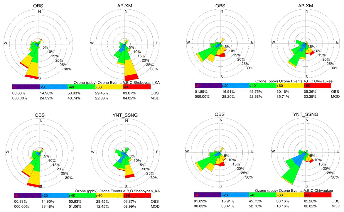
Figure 9 Observed (OBS) and simulated wind roses using 1 h ozone and wind directions at the Sheboygan Kohler-Andrae (KA) AQS monitor (551170006; four plots on the left) and Chiwaukee Prairie AQS monitor (550590019; four plots on the right) for the 1.3 km AP-XM (upper rows) and YNT_SSNG (lower rows) CMAQ simulations during high-ozone events A, B, and C. Wind directions are divided into 22.5^∘ resolution bins, and the percentage of winds within each directional bin is indicted by the percentages on the wind rose plots. The colors within each wind direction bin indicate the distribution of observed and simulated ozone within 20 ppbv bins, as indicated by the color bars. The overall percentage of observed (OBS) and simulated (AP-XM or YNT_SSNG) ozone within each ozone bin is indicated below the color bar for each site and simulation.

3.2.3 The 1 h ozone concentration and wind direction during high-ozone events A, B, and C

While the ozone wind roses presented above provide a comparison of the joint distribution of simulated and observed winds and ozone at these two stations, they do not provide a quantitative estimate of the errors in the simulations. In this section, we have binned the simulated and observed ozone and wind direction to provide a more quantitative characterization of the simulated biases. Figure 10 shows box-and-whisker plots of 1.3 km YNT_SSNG and AP-XM CMAQ ozone simulations and 1 h averaged observed ozone at Chiwaukee Prairie and Sheboygan KA during high-ozone events A, B, and C. Both simulations show systematic high biases for lower observed ozone concentrations (≲ 40 ppbv) and low biases for higher-ozone concentrations (>50 ppbv) at both sites. These results are consistent with the 8 h maximum ozone biases for the 1.3 km domain wide comparison (Fig. 1). The AP-XM simulation shows better agreement with observed ozone for the highest ozone (>85 ppbv) at both sites during high-ozone events but shows a wider spread in the simulated distribution within each of these high observed ozone bins at Chiwaukee Prairie. The AP-XM and YNT_SSNG CMAQ simulations show similar distributions for observed ozone less than 80 ppbv.

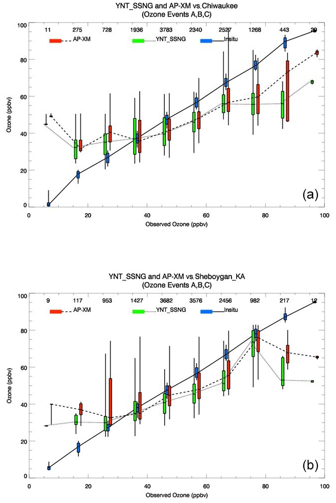
Figure 10 Box-and-whisker plots showing the binned median ozone concentrations from the 1.3 km AP-XM (dashed lines) and YNT_SSNG (dotted lines) CMAQ simulations and observed ozone (solid lines) at Chiwaukee Prairie (a) and Sheboygan KA (b) during high-ozone events A, B, and C. The vertical boxes show the 50 % and the vertical lines show the 95 % ranges of distributions for the AP-XM (red) and YNT_SSNG (green) CMAQ simulations and observed ozone (blue). The total observed count within each 5 ppbv bin is indicated at the top of each panel.

Figure 11 shows box-and-whisker plots of 1.3 km YNT_SSNG and AP-XM CMAQ wind direction simulations and 1 h averaged observed wind direction for wind speeds greater than 1 m s⁻¹ at Chiwaukee Prairie and Sheboygan KA during high-ozone events A, B, and C. The 1 m s⁻¹ threshold was included to reduce the impact of light and variable winds at these sites. Both simulations show a large westerly median bias and large variations in wind direction when the observed winds have an easterly component (0–180^∘) at Chiwaukee Prairie. This could be associated with errors in the timing of the arrival of the lake breeze, but a more detailed analysis along the lines of Wagner et al. (2022) would have to be performed to confirm this. Winds with an easterly component account for 30 % of the observed wind directions at this site. Both simulations show a smaller easterly bias in the median wind direction when the observed winds have a westerly component (180–360^∘) at Chiwaukee Prairie, but the YNT_SSNG simulation is in better agreement with observations during these periods. The AP-XM simulation shows small easterly biases when the observed winds have an easterly component at Sheboygan KA, while the YNT_SSNG simulation still shows some westerly biases in the median wind direction for these cases. Both simulations show somewhat larger easterly median biases when the observed winds have a westerly component at Sheboygan KA, but the YNT_SSNG simulation is better agreement with observations for these cases.

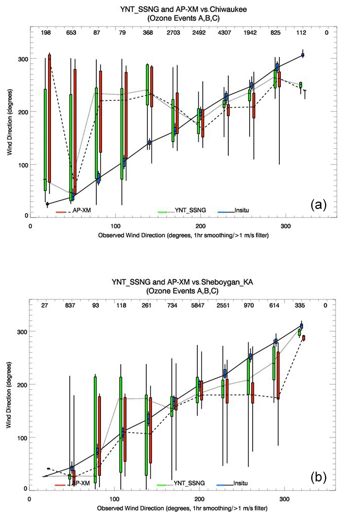
Figure 11 Box-and-whisker plots showing the binned median wind direction from the 1.3 km AP-XM (dashed lines) and YNT_SSNG (dotted lines) CMAQ simulations and observed wind direction (solid lines) at Chiwaukee Prairie (a) and Sheboygan KA (b) during high-ozone events A, B, and C. The vertical boxes show the 50 % and the vertical lines show the 95 % ranges of distributions for the AP-XM (red) and YNT_SSNG (green) CMAQ simulations and 1 h averaged observed wind direction (blue). The total observed count within each 20^∘ resolution bin is indicated at the top of the figures.

3.2.4 GeoTASO comparisons during high-ozone events A, B, and C

Here, we use GeoTASO (Nowlan et al., 2016) NO₂ and HCHO column measurements to verify ozone precursors within the YNT_SSNG and AP-XM simulations during high-ozone events A, B, and C. Figure 12 shows the results of the NO₂ column analysis. Compared to observed NO₂ column measurements, the YNT_SSNG and AP-XM simulations have a similar correlation (0.60 vs. 0.57) and the YNT_SSNG has a substantially reduced bias (0.17×10¹⁵ vs. 0.31×10¹⁵ mol cm⁻²). Figure 13 shows the results of the HCHO column analysis. Compared to observed HCHO column measurements, the YNT_SSNG has a lower correlation than the AP-XM simulation (0.24 vs. 0.33) and a larger bias (3.1×10¹⁵ vs. 2.3×10¹⁵ mol cm⁻²).

Nowlan et al. (2018) used comparisons between the GEOstationary Coastal and Air Pollution Events (GEO-CAPE) Airborne Simulator (GCAS, which is similar to the GeoTASO instrument) NO₂ and HCHO retrievals and columns estimated from airborne in situ NO₂ and HCHO profiles to estimate mean precisions of 1×10¹⁵ and 19×10¹⁵ mol cm⁻² for the native (250 m) resolution NO₂ and HCHO retrievals, respectively. The LMOS 2017 GeoTASO radiances were co-added onto a 1 km grid during the 2017 LMOS campaign, so we anticipate that the precision of the 1 km retrievals is better by a factor of 2. Given the relatively high precision of GeoTASO NO₂ compared to the column amounts observed during high-ozone events A, B, and C, we conclude that the high bias in NO₂ columns in the AP-XM simulation is significant, with more AP-XM NO₂ columns found outside the estimated $\pm \mathrm{0.5}\times {\mathrm{10}}^{\mathrm{15}}$ mol cm⁻² precision range than found in the YNT_SSNG simulation. We have less confidence in the significance of the differences between the YNT_SSNG and AP-XM HCHO columns relative to the GeoTASO retrievals, since the observed HCHO columns are on the order of the precision of the instrument (10×10¹⁵ mol cm⁻²), and the biases in the HCHO column simulations are both mostly less than the GeoTASO precision during high-ozone events A, B, and C. Overall, our results show that the YNT_SSNG simulation has an improved representation of NO₂, which is a primary ozone precursor, during these high-ozone events.

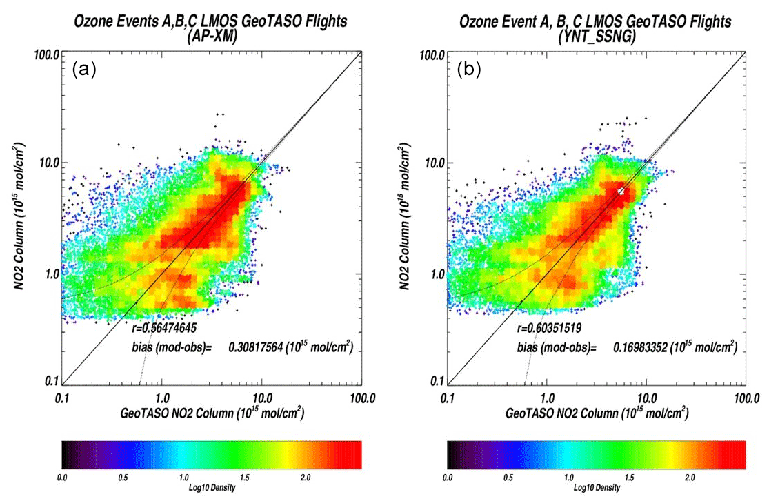
Figure 12 Scatterplots of 1.3 km AP-XM (a) and YNT_SSNG (b) NO₂ columns versus GeoTASO NO₂ columns (×10¹⁵ mol cm⁻²) during LMOS 2017 high-ozone events A, B, and C. The dashed lines show the precision (±) of the GeoTASO NO₂ columns.

Figure 13 Same as Fig. 10 but for HCHO columns.

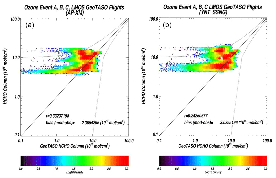
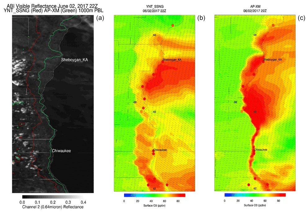
Figure 14 Advanced Baseline Imager (ABI) visible (0.64 µ) reflectance (a), YNT_SSNG surface ozone (ppbv; b), and AP-XM surface ozone (ppbv; c) at 22:00 GMT on 2 June 2017. Observed AQS ozone concentrations at 22:00 GMT are shown as colored circles. Location of 1 km YNT_SSNG (red) and AP-XM (green) PBL heights are also shown in the ABI (a). The locations of the Sheboygan KA and Chiwaukee Prairie AQS monitors are labeled in each of the panels.

3.3 The 2 June 2017 ozone exceedance event

The only ozone exceedance event that had significant inland penetration of the lake breeze at both Chiwaukee and Sheboygan KA during LMOS 2017 occurred on 2 June 2017 (Stanier et al., 2021; Wagner et al., 2022). The simulations on this day most clearly illustrate the differences between the AP-XM and YNT_SSNG results. Figure 14 shows the observed visible (0.64 µ) reflectance from the Advanced Baseline Imager (ABI) on the NOAA Geostationary Operational Environmental Satellite Program (GOES)-16 satellite and surface ozone concentrations from the YNT_SSNG and AP-XM simulations, respectively, at 22:00 GMT (17:00 CDT) on 2 June 2017. To delineate the simulated continental convective and stable maritime boundary layers, we also show where the YNT_SSNG and AP-XM simulated PBL heights are >1 km (Fig. 14a; see the red or green lines). These contours roughly correspond to the westernmost edge of the simulated marine boundary layer and indicate the extent of the penetration of the lake breeze circulation. The ABI visible reflectances clearly show where the stable marine boundary layer suppresses the formation of fair-weather cumulus clouds, which form within the turbulent continental boundary layer and are evident to the west of the YNT_SSNG 1 km PBL height contour. The YNT_SSNG simulation shows a more extensive penetration of high-ozone concentrations inland, which is in agreement with the extent of the penetration of the marine boundary layer. In contrast, the AP-XM simulation shows very little penetration of the stable marine boundary layer. This lake breeze penetration has a significant impact on the simulated surface ozone distributions. While the YNT_SSNG simulation shows deeper penetration of the lake breeze circulation, it also leads to somewhat lower surface ozone concentrations near the shoreline, leading to underestimates of the observed ozone concentrations at this time.

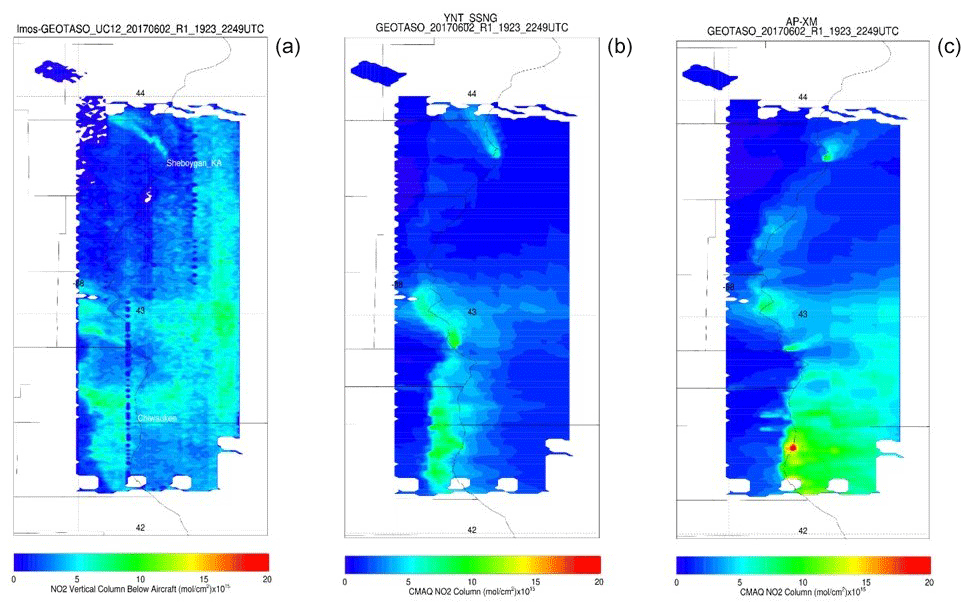
Figure 15 GeoTASO (a), YNT_SSNG (b), and AP-XM (c) NO₂ (×10¹⁵ mol cm⁻²) column on 2 June 2017. The location of the Sheboygan KA AQS station is indicated in panel (a).

Figure 15 shows comparisons between airborne GeoTASO, YNT_SSNG, and AP-XM NO₂ column along the western shore of Lake Michigan on 2 June 2017. Comparisons with NO₂ column distributions provide a means of comparing the fidelity of the lake breeze transport of ozone precursors during this high-ozone event. Observed NO₂ columns peak near 10×10¹⁵ mol cm⁻² and show the penetration of the high NO₂ column amounts inland by the lake breeze circulation, which is consistent with the ABI visible reflectances. The observed NO₂ columns also show enhancements over the lake on the eastern part of the GeoTASO raster pattern that are best captured by the AP-XM simulation. The GeoTASO NO₂ columns show peak amounts of 10×10¹⁵ mol cm⁻² and significant inland penetration of higher NO₂ columns over the southern portion of the flight track. The YNT_SSNG NO₂ column shows similar peak amounts and shows similar, but not as far inland, penetration of the high NO₂ columns. The AP-XM NO₂ column shows localized NO₂ columns over 15×10¹⁵ mol cm⁻² along the Lake Michigan shoreline and does not predict as much onshore penetration. The narrow plume of higher GeoTASO NO₂ column extending to the northwest from the coast north of the Sheboygan KA AQS monitor is a signature of the Edgewater Generating Station. The YNT_SSNG and AP-XM simulations also show this plume, but the YNT_SSNG simulation does a better job of capturing the northwestward transport of the plume, while the AP-XM simulation shows transport of this narrow plume to the north-northeast.

Figure 16 shows comparisons between airborne GeoTASO, YNT_SSNG, and AP-XM HCHO column along the western shore of Lake Michigan on 2 June 2017. HCHO columns vary much less spatially than NO₂ columns, despite both anthropogenic and biogenic VOC emissions influencing the former, while the latter is primarily associated with anthropogenic emissions. Both simulations capture the observed north-to-south positive gradient, thus providing some confidence in the larger-scale gradients. However, the GeoTASO HCHO measurements show values in excess of 10×10¹⁵ mol cm⁻² over Lake Michigan that are not captured in either the YNT_SSNG or AP-XM HCHO column simulations. Given the lower-precision GeoTASO HCHO columns, the differences between the YNT_SSNG and AP-XM HCHO columns are difficult to quantify with these measurements. We note large differences between simulated and observed GeoTASO NO₂ and HCHO over the eastern portion of the observations. These observations were collected later during the flight and therefore subject to larger uncertainties related to the impact of stratospheric NO₂ and ozone absorption interferences.

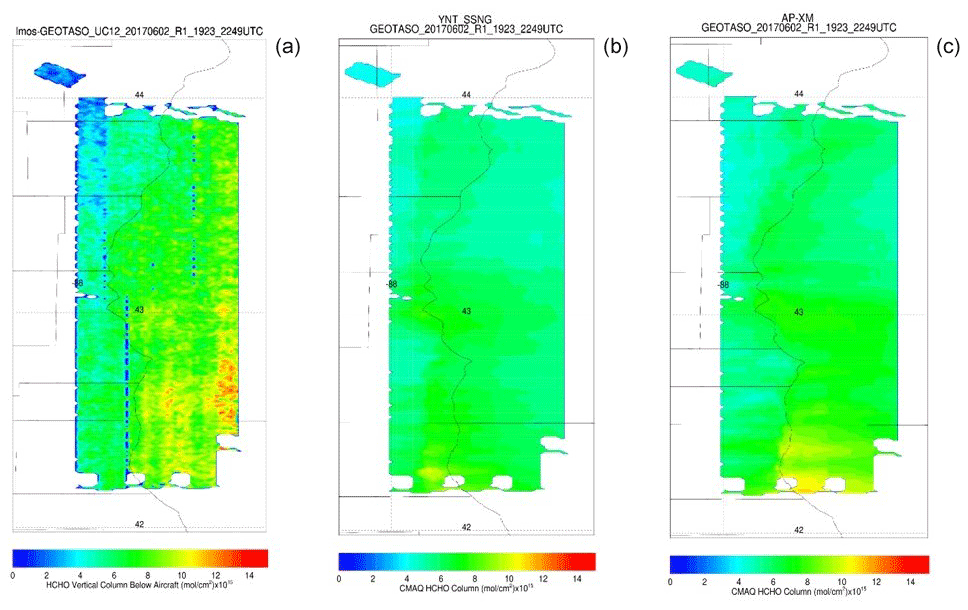
Figure 16 GeoTASO (a), YNT_SSNG (b), and AP-XM (c) HCHO (×10¹⁵ mol cm⁻²) column on 2 June 2017.

Figure 17 shows comparisons between observed time–height cross sections of thermodynamic (temperature) and kinematic (wind) distributions at Sheboygan, WI, during the 2 June 2017 ozone exceedance event. Observed temperatures are obtained from the University of Wisconsin–Madison atmospheric emitted radiance interferometer (AERI) instrument (Knutson et al., 2004a, b), while wind direction and speed are obtained from a HALO Photonics Doppler wind lidar instrument. Both of these instruments were deployed at the Sheboygan, WI, ground site during LMOS 2017 (Stanier et al., 2021; Wagner et al., 2022). AERI temperatures show a well-defined nocturnal boundary layer with a thin layer of cold temperatures below 100 m a.g.l. and a warmer layer extending up to approximately 600 m. The continental convective boundary layer begins to form as the Sun rises (∼ 12:00 GMT or 07:00 CDT). This is evident in the warmer surface temperatures near 15:00 GMT (10:00 CDT). The AERI measurements show a new shallow layer of cooler air below 50 m arriving at 17:00 GMT (12:00 CDT), which is associated with the stable marine boundary layer. Observed wind directions are out of the NW prior to 15:00 GMT at 7 m s⁻¹, rapidly diminish at around 15:00 GMT, and then switch to the SE at around 18:00 GMT (13:00 CDT) when the lake breeze reaches Sheboygan, WI. Both simulations show an easterly bias during the observed NW winds, which is consistent with the overall statistics during ozone events A, B, and C shown in Fig. 11. The YNT_SSNG simulation captures the thermal structure of the nocturnal boundary layer (temperature differences are less than 2 ^∘C below 100 m) and the timing of the arrival of the maritime boundary layer but underestimates the near-surface (below 200 m) convective boundary layer temperatures by up to 10 ^∘C at 15:00 GMT. The AP-XM simulation shows significant (temperature differences are greater than 5 ^∘C below 100 m) overestimates of the nocturnal boundary layer temperatures and shows a gradual warming of temperatures below 200 m after 15:00 GMT, resulting in large (greater than 7 ^∘C) overestimates in temperatures and no evidence of the cooler lake breeze. Both simulations underestimate the observed increase in wind speed prior to the arrival of the lake breeze by ∼2 m s⁻¹. The YNT_SSNG simulation shows a more rapid shift in wind direction associated with the arrival of the lake breeze than the AP-XM simulation, but the timing of the switch in wind direction is about 3 h too early in the YNT_SSNG simulation. This results in errors in wind speeds of up to 5 m s⁻¹ near 200 m in the YNT_SSNG simulation prior to the observed reduction in wind speed at 15:00 GMT. The observed depth of the wind shift is underestimated in both simulations, but the YNT_SSN simulation does a better job of capturing the vertical extent of the wind shift and reduction in wind speed above 200 m. This is most evident above 400 m, where the AP-XM wind speeds are underestimated by up to 5 m s⁻¹.

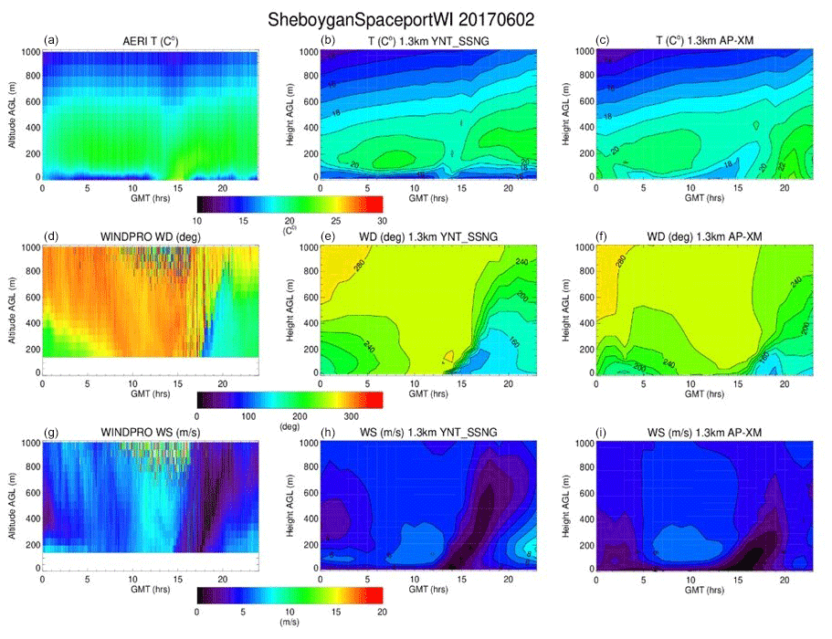
Figure 17 Time–height curtains of observed (a, d, g), YNT_SSNG (b, e, h), and AP-XM (c, f, i) temperature (T in ^∘C; a, b, c), wind direction (WD in degrees; d, e, f), and wind speed (WS in m s⁻¹; g, h, i) at Sheboygan, WI, on 2 June 2017. Observed temperature is from University of Wisconsin–Madison AERI and observed winds are from the HALO Photonics Doppler wind lidar instrument.

Figure 18 shows comparisons between observed time–height cross sections of thermodynamic (temperature) and kinematic (wind) distributions at Zion, IL, during the 2 June 2017 ozone exceedance event. Observed temperatures are obtained from the ground-based microwave radiometer while wind direction and speed were observed using a Sound Detection and Ranging (Sodar) instrument, both of which were provided by the University of Northern Iowa. Both of these instruments were deployed at the Zion, IL, ground site during LMOS 2017 (Stanier et al., 2021; Wagner et al., 2022). Microwave temperatures show a well-defined nocturnal boundary layer, with a thin layer of cooler temperatures below 100 m that is similar to Sheboygan, WI (Fig. 17), but not as cold. The continental convective boundary layer begins to form as the Sun rises (∼ 12:00 GMT or 07:00 CDT). This is evident in the warmer surface temperatures near 15:00 GMT (10:00 CDT). In contrast to Sheboygan, the microwave temperatures do not show a signature of the cooler air associated with the stable marine boundary layer. This may be due to the fact that the Zion, IL, site is further inland than the Sheboygan site and that turbulent heat fluxes from the warmer land surface warm the marine layer. The Sodar wind direction shows a sharp transition from southwesterly to southeasterly winds and a rapid reduction in wind speed (from over 10 m s⁻¹ to less than 5 m s⁻¹) at 15:00 GMT, which is associated with the arrival of the lake breeze at the Zion, IL, site. Both the YNT_SSNG and AP-XM simulations overestimate the temperature within the nocturnal boundary layer, with the AP-XM showing somewhat larger warm biases (>5 ^∘C) below 100 m compared to YNT_SSNG (<5 ^∘C). The YNT_SSNG simulation captures the development of the continental convective boundary layer better than the AP-XM simulation, which underestimates the observed temperatures by 5–7 ^∘C below 100 m between sunrise (12:00 GMT) and 15:00 GMT (10:00 CDT). This cold bias persists until 20:00 GMT (15:00 CDT) in the AP-XM simulation. The YNT_SSNG simulation shows some evidence of a cooler lake breeze moving over the Zion, IL, site that leads to a cold bias of 5–7 ^∘C at 20:00 GMT. The YNT_SSNG simulation more accurately captures the timing of the wind shift at 15:00 GMT, which is delayed by nearly 3 h in the AP-XM simulation. Wind speeds are similar in both simulations, although the YNT_SSNG simulation shows slightly higher (8 m s⁻¹ versus 7 m s⁻¹) wind speeds prior to the arrival of the lake breeze and stronger (6 m s⁻¹ versus 3 m s⁻¹) low-level winds after 20:00 GMT, which are in better agreement with the Sodar measurements.

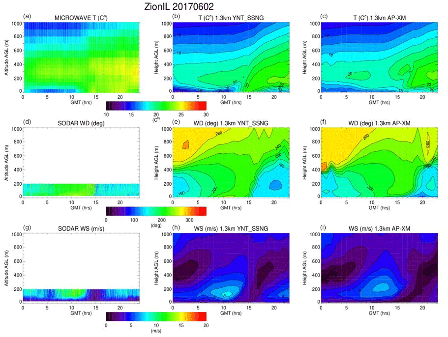
Figure 18 Time–height curtains of observed (a, d, g), YNT_SSNG (b, e, h), and AP-XM (c, f, i) temperature (T in ^∘C; a, b, c), wind direction (WD in degrees; d, e, f), and wind speed (WS in m s⁻¹; g, h, i) at Zion, IL, on 2 June 2017. Observed temperatures were obtained using a microwave radiometer and observed winds are from a Sodar instrument, which were provided by Alan Czarnetski at the University of Northern Iowa.

4 Discussion and conclusions

We have conducted an evaluation of two model simulations employing differing meteorological inputs, with the goal of identifying a model configuration best suited for characterizing the spatial and temporal variability in the ozone and its precursors in locations where lake breezes commonly affect local air quality along the Lake Michigan shoreline. We focus on the period of the LMOS campaign, 22 May–22 June 2017, using the innermost grid of a triple-nested simulation around Lake Michigan, with a horizontal resolution of 1.3 km. The AP-XM simulation used the same boundary layer and surface physics that are used within CMAQ for WRF inputs. Our YNT_SSNG simulation used different WRF parameterizations and constraints from satellite observations of the green vegetation fraction and soil temperature and moisture, as detailed by Otkin et al. (2023).

Both model simulations reasonably capture the observed daily maximum 8 h average ozone amounts over the study period; however, both simulations underestimated ozone amounts at times with high ozone and overestimated ozone when observed amounts were low. These ozone biases are consistent with those simulated by Baker et al. (2023). Both model simulations also perform similarly on an hourly basis on high-ozone days. We find that the AP-XM simulation better represents hourly ozone when observed amounts are high (80–90 ppbv), and the YNT_SSNG simulation overall biases are generally smaller (less negative) than those of the AP-XM simulation. Both simulations also tend to underestimate the amounts of the ozone precursor HCHO, with smaller (less negative) biases in the YNT_SSNG simulation. This is despite the fact that the YNT_SSNG uses a more realistic and lower (relative to climatology) green vegetation fraction (which would tend to reduce biogenic VOC emissions), suggesting that anthropogenic HCHO emissions may be playing a more important role in HCHO concentrations in the YNT_SSNG simulation. Both simulations significantly underestimate isoprene, with larger (more negative) biases in the YNT_SSNG simulation. This is also consistent with the use of more realistic and lower (relative to climatology) green vegetation fraction in the YNT_SSNG simulation. We find that the simulations are less similar in their representation of NO₂ amounts; while the AP-XM simulation tends to underestimate NO₂ at monitor sites, the YNT_SSNG simulation has an overall high (positive) bias.

Since the simulations use identical anthropogenic emissions and chemistry, the differences in modeled ozone and precursors are linked to any differences in biogenic emissions resulting from the input meteorology and from differences in boundary layer mixing and horizontal and vertical transport. In Part 1 of this study, Otkin et al. (2023) noted that the AP-XM simulation had an overall low bias in wind speed, the YNT_SSNG simulation had a positive bias, and the simulations had a similar RMSE. Here, we find many similarities between simulations on high-ozone days. At Chiwaukee Prairie, we find that both simulations capture the highest-ozone amounts transported from the SSE. On high-ozone days at Sheboygan KA, observed winds tend to be SSW, while both models show highest-ozone amounts transported from the SSE. At Chiwaukee Prairie, both simulations tend to have a westerly bias when observed winds have an easterly (onshore) component.

We find greater differences in column amounts of ozone precursors. The AP-XM simulation has a negative bias in near-surface NO₂ at Sheboygan, a high bias in near-surface NO₂ at Zion, IL, a positive bias in column NO₂ amounts, and elevated column amounts concentrated along the Lake Michigan shoreline during the ozone exceedance event on 2 June. The YNT_SSNG simulation has a small positive bias in NO₂ column amounts, with elevated column amounts extending further inland on the lake-breeze-enhanced ozone event on 2 June. While these differences reflect the parameterizations used to generate input meteorology, differences in vertical mixing, and ensuing column amounts of NO₂ and HCHO discussed here, they are further complicated by CMAQ using the ACM2 parameterization for vertical diffusion. This is a mismatch for the YNT_SSNG simulation that influences our evaluation, since it leads to differences in boundary layer mixing. Still, the NO₂ column comparisons provide support for the improved representation of the lake breeze transport of ozone precursors in the YNT_SSNG simulation. Future model comparisons with upcoming geostationary observations will allow for more extensive analysis to assess the model performance with respect to the diurnal evolution of precursors during ozone events.

Our thermodynamic and kinematic comparison of the AP-XM and YNT_SSNG simulations show improved representation of not only the extent but also of the timing of the lake breeze in the YNT_SSNG simulation at Sheboygan, WI, and Zion, IL, for the 2 June 2017 ozone episode. This is consistent with the meteorological analysis presented in Part 1 of this study, where the YNT_SSNG had a better representation of diurnal patterns (Otkin et al., 2023). However, we note that the meteorological inputs to our CMAQ simulations are hourly, as is typically used in air quality modeling studies. Both simulations would likely benefit from sub-hourly winds, given the rapid changes that can occur in the presence of lake and land breeze circulations. For this reason, a more tightly coupled model such as WRF–CMAQ (Wang et al., 2021) would be better suited for a goal of better simulating the fine temporal and spatial scales of lake breeze transport and chemistry.

This analysis complements other studies in the evaluation of the impact of changing meteorological inputs and parameterizations on air quality in a complex environment. Appel et al. (2014) also found improved representation of ozone in environments with bay and sea breezes with the addition of high-resolution sea surface temperature (SST) into the WRF and CMAQ modeling framework. Cheng et al. (2012) underscored the importance of PBL parameterization in simulating land–sea breezes and their impacts on near-surface ozone. Similar to our work, Banks and Baldasano (2016) evaluated the impacts of PBL parameterizations on air quality and also found ambiguous results, with the simulation using the YSU PBL better capturing observed NO₂ and the simulation using the ACM2 PBL better capturing observed ozone. Future work will be able to take advantage of ongoing improvements to both WRF and CMAQ, such as an update to the calculation of vegetative fraction and Pleim–Xu LSM soil parameters in WRF (Appel et al., 2021), and should explore the relationships among the spatial and temporal resolution of meteorological parameterizations themselves, along with those of the modeling framework.