Climatology of aerosol properties at an atmospheric monitoring site on the northern California coast

Between April 2002 and June 2017, the Global Monitoring Laboratory (GML) of the National Oceanic and Atmospheric Administration (NOAA) made continuous measurements of a suite of in situ aerosol optical properties at a long-term monitoring site near Trinidad Head (THD), California. In addition to aerosol optical properties, between 2002–2006 a scanning humidograph system was operated, and inorganic ion and total aerosol mass concentrations were obtained from filter measurements. A combined analysis of these datasets demonstrates consistent patterns in aerosol climatology and highlights changes in sources throughout the year. THD is predictably dominated by sea salt aerosols; however, marine biogenic aerosols are the largest contributor to PM₁ in the warmer months. Additionally, a persistent combustion source appears in the winter, likely a result of wintertime home heating. While the influences of local anthropogenic sources from vehicular and marine traffic are visible in the optical aerosol data, their influence is largely dictated by the wind direction at the site. Comparison of the THD aerosol climatology to that reported for other marine sites shows that the location is representative of clean marine measurements, even with the periodic influence of anthropogenic sources.

1 Introduction

Aerosol particles affect the radiative balance both by scattering and absorbing solar radiation and by influencing the properties of clouds (IPCC, 2013). In order to separate out the contribution of anthropogenic aerosol to aerosol radiative forcing, the impact of natural aerosol particles must also be quantified (Andreae, 2007). Because the Earth's surface is dominated by oceans, marine aerosols are a dominant contributor to natural background aerosol levels (Murphy et al., 1998; Jaeglé et al., 2011), although their contribution is variable in time and space. Marine aerosols can be generated both through wave breaking – which generates sea salt aerosols consisting of both soluble ions and organic material – and through gas-to-particle conversion of volatile organic compounds (VOCs) generated by biogenic activity, leading to marine biogenic aerosols (O'Dowd and de Leeuw, 2007; Fitzgerald, 1991). The aerosol in coastal regions may be subject to significant impacts from local and/or regional anthropogenic sources, as well as long-range transport, particularly in the Northern Hemisphere (Andreae, 2007); this can make it difficult to definitively characterize the natural marine aerosol. Understanding the marine aerosol is critical not only for assessing direct aerosol forcing of a major natural aerosol type but also because marine aerosol plays a key role in cloud formation over much of the globe (Mayer et al., 2020; Hodshire et al., 2019; Carslaw et al., 2010).

Measurements over the open ocean (where anthropogenic influence is less pronounced) typically require mobile platforms such as instrumented ships or aircraft, so remote coastal locations are often used as a surrogate for sampling the marine atmosphere (O'Dowd et al., 2014; Bates et al., 1998; Brunke et al., 2004; Wood et al., 2015). An advantage that surface-based coastal site measurements have over sampling from mobile platforms is that long-term, continuous information can be obtained, allowing for the development of representative climatologies on variable timescales (diurnal to annual) and the evaluation of long-term trends. Such measurements can then be used to evaluate models, but whether the measurements are representative of a clean marine environment should also be assessed (O'Dowd et al., 2014; Wang et al., 2018).

An established, long-term observatory can provide a platform for multiple instrument suites probing different aspects of the atmosphere. Long-term atmospheric monitoring deployments are (typically) limited in measurement scope to robust and proven standalone techniques, which is in contrast to field campaign efforts, which frequently utilize state-of-the-art and/or prototype instruments that only need to be operated for a short time and are attended by on-site scientists. Long-term datasets of atmospheric constituents provide an opportunity to describe inter-annual variability and climatology on a variety of timescales, to identify trends, and to develop a robust understanding of relationships amongst the measured parameters, which may not be possible from short-term studies. Analyses of extended time series of atmospheric data can be used to provide a context for field campaign observations (Brock et al., 2011; Leaitch et al., 2020), assess model simulations (Spracklen et al., 2010; Browse et al., 2012), evaluate the effectiveness of pollution control legislation and exposures (Murphy et al., 2008), and answer scientific questions related to sources, atmospheric processes, and the impacts of extreme events (Sorribas et al., 2015; Hallar et al., 2015).

In April 2002, a surface monitoring site was established at Trinidad Head (THD), near the small town of Trinidad on the northern coast of California, in order to study properties of atmospheric constituents (e.g., aerosol particles and ozone) entering the USA prior to influence by North American sources. The start of measurements at THD coincided with the 1-month intensive field campaign, Intercontinental Transport and Chemical Transformation (ITCT 2K2), aimed at understanding how (relatively) short-lived species such as aerosol particles can be transported and detected far from their source and how these species change during transport (Parrish et al., 2004). While it was found that surface measurements at THD were not ideal for studying long-range transport (VanCuren et al., 2005), it was a reasonable location for making measurements of the clean marine environment. Thus, the site remained active with a smaller suite of measurements as a long-term National Oceanic and Atmospheric Administration (NOAA) Global Monitoring Laboratory (GML) monitoring site for an additional 15 years and closed down in June 2017. This paper focuses on an analysis of surface aerosol measurements observed at THD over the 2002–2017 period of measurements and addresses two main questions in the context of remote marine observations:

1. What is the climatology (seasonal and diurnal cycles) of the aerosol chemical and optical properties at THD?

2. Are there any systematic relationships between the aerosol chemical composition and aerosol optical properties?

The discussion of these results assesses implications in terms of aerosol sources and how well THD represents a clean marine site.

2 Methods

The measurements described here were conducted at the atmospheric monitoring station on Trinidad Head, California (41.054^∘ N, 125.151^∘ W; 107 m a.s.l. – above sea level). The site is ∼ 370 km (∼ 230 miles) north of the San Francisco Bay area (population ∼ 8.7 million) and ∼ 350 km (∼ 220 miles) south of Eugene, Oregon (population ∼ 170 000), making it a location relatively remote from large local and regional sources of anthropogenic pollution (Fig. 1). The site is ∼ 22 km (∼ 13.5 miles) north of the smaller city of Arcata (population ∼ 19 000) and directly southwest of the city of Trinidad (population ∼ 300). Aerosol chemical filters were collected over a 4-year period from 15 April 2002–May 2006, and the aerosol optical measurements reported here cover a ∼ 15-year period from 15 April 2002–1 June 2017. Other measurements took place over more limited time frames. Table 1 describes the aerosol instruments operated at Trinidad Head (THD) and their periods of operation.

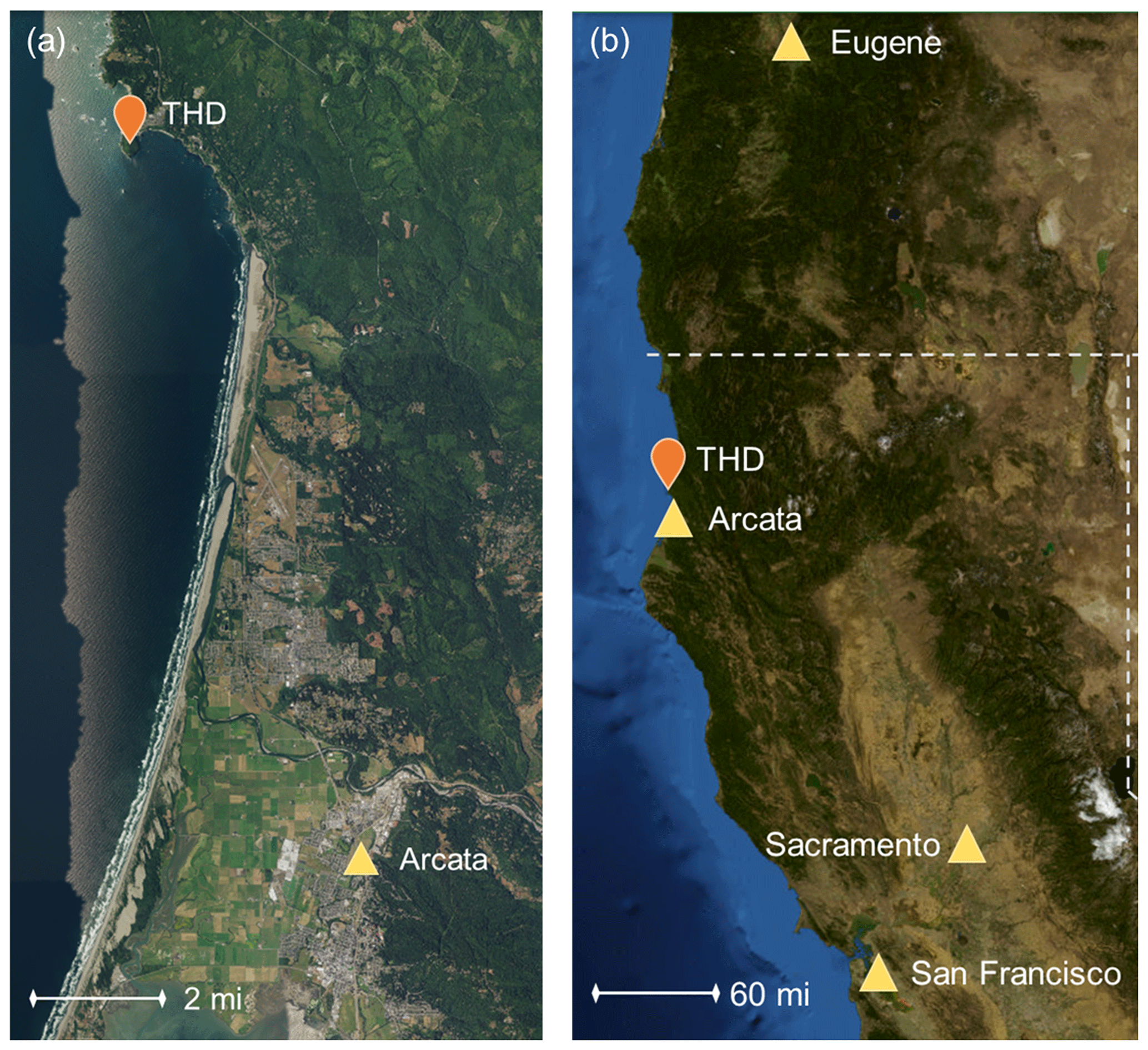
Figure 1 Maps of the measurement site in relation to major cities. A smaller scale is shown in panel (a) of the more local coastline, and a larger scale in panel (b) shows the broader area. Maps were constructed using images and information from the United States Geological Survey's program of The National Map (U.S. Geological Survey, 2019).

Table 1 Instrumentation at Trinidad Head.

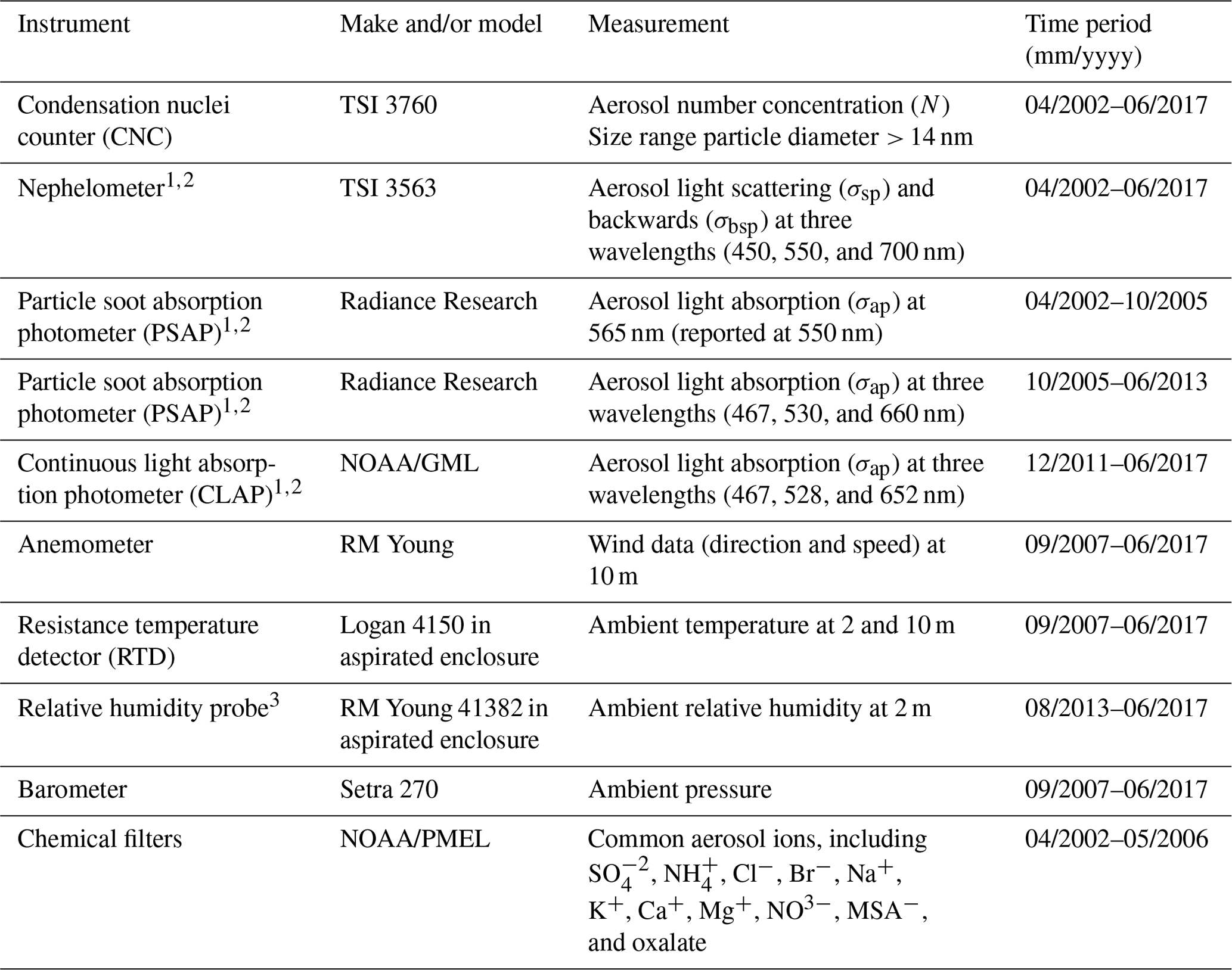
¹ These measurements measured at two size cuts, namely PM₁ and PM₁₀. ² Correction methods used for these instruments are outlined in Anderson and Ogren (1998) for the nephelometer and Bond et al. (1999) and Ogren (2010) for the PSAP and CLAP. ³ Ambient RH measurements prior to August 2013 were invalid.

2.1 Aerosol inlet system

The aerosol inlet and system at THD are the standard NOAA design and have been described in detail in other papers (Sheridan et al., 2001; Delene and Ogren, 2002; Sherman et al., 2015), so only a brief description is given here. The sampling stack was 10 m tall, constructed of 8 in. (20.32 cm) inner diameter PVC (polyvinyl chloride) pipe. A rain hat prevented precipitation from entering sample stack; the rain hat design was changed in March 2010. A total airflow of ∼ 1000 L min⁻¹ entered the stack. Most of this airflow (850 L min⁻¹) was excess air, while the remaining 150 L min⁻¹, the sample flow, was pulled through a gently heated 2 in. (5.08 cm) stainless-steel pipe at the base of the sampling stack and fed into a five-port flow splitter. The heating applied to the stainless-steel tube was used to lower the relative humidity (RH) of the sample to comply with Global Atmosphere Watch (GAW) sampling protocols of keeping sample RH below 40 % (WMO/GAW, 2016). At THD, 30 L min⁻¹ of the splitter sample flow was routed to the aerosol optical properties measurement system, 30 L min⁻¹ went to the chemical filter measurements, and 30 L min⁻¹ was used to monitor the RH in the stainless-steel inlet and control the heat to lower that RH when necessary. The remaining two lines (three lines after discontinuation of the chemical measurements in 2006) of 30 L min⁻¹ flow were not used and went directly from the flow splitter to the pump box.

For the aerosol optical property measurements, the 30 L min⁻¹ of the sample flow was further warmed by a secondary heater when necessary to maintain the system's RH at less than 40 %. The average temperature downstream of the secondary heater was 22 ± 4 ^∘C during site operation (20 ± 3, 20 ± 3, 23 ± 5, and 22 ± 3 ^∘C in the winter, spring, summer, and fall, respectively). Downstream of the secondary heater, a switched impactor system provided size-segregated measurements. The sample air first flowed through a Berner-type multi-jet cascade 10 µm impactor (∼ 7 µm aerodynamic diameter; Berner et al., 1979). An electronic ball valve was used to switch between a direct sample line to the instruments and a second Berner-type impactor with a size cut of 1 µm (∼ 0.7 µm aerodynamic diameter). Here, the 10 µm size cut is referred to as the total size cut or PM₁₀, while the 1 µm size cut is referred to as the submicron size cut or PM₁. Switching between PM₁₀ and PM₁ size cuts occurred every 6 min between April 2002 and May 2004, every 30 min between May 2004 and March 2006 to optimize humidograph operations, and then back to switching every 6 min after the humidograph was removed until the station closed in June 2017.

2.2 Aerosol chemical composition

For the first 4 years of measurements at the site, an additional 30 L min⁻¹ of the flow from the flow splitter was pulled through a filter carousel system used to collect aerosol on filters for chemical analysis. The filter carousel system used the same PM₁₀ and PM₁ impactors as the aerosol optical system. Results from an identical system were described in Quinn et al. (2002). The filters were analyzed by the Pacific Marine Environmental Laboratory (PMEL). More details of their analysis can be found in Quinn et al. (2000). The samples were analyzed using ion chromatography for major ionic species, including SO${}_{\mathrm{4}}^{\mathrm{2}-}$, NH${}_{\mathrm{4}}^{+}$, Cl⁻, Br⁻, Na⁺, K⁺, Ca⁺, Mg⁺, NO³⁻, methanesulfonic acid (MSA⁻), and oxalate. Aerosol mass concentrations for both PM₁ (daily) and for PM between 1 µm < D_p​​​​​​​ < 10 µm (weekly) were obtained. The PM₁ data were then averaged over the weekly sampling time of the 1–10 µm PM samples, and the two masses were added together to achieve a PM₁₀ mass that could be compared to the optical data. It is important to note that some fraction of the NO³⁻ mass may have been driven off through the heating of the sampled air described above and, therefore, could be underestimated in this work (Bergin et al., 1997). For the first ∼ 1.5 years of the program, local contamination episodes were identified when the wind was from the eastern and southeastern sectors (specifically 56–186^∘) and the chemical filtering system was bypassed. In addition to the wind direction, the particle number concentration (N) was used to identify periods of local contamination (N > 8000 cm⁻³; Sheridan et al., 2016). Chemical sampling was switched off during contamination periods. Identification of contamination using wind sector was stopped on 7 October 2003. It was determined that the airflow around the site was heavily influenced by the local topography and was leading to the elimination of non-contaminated data. Ion concentrations were compared to elemental measurements made with a rotating drum impactor that operated at THD during the spring of 2002 (Sect. S1 in the Supplement). Additionally, simple outlier testing was done on the filter data with monthly and seasonal analysis based on the interquartile range (IQR). Data points were defined as outliers and were not included in analysis if they fell outside the range of $Q\mathrm{25}-(\mathrm{IQR}\times \mathrm{1.5})$ to $Q\mathrm{75}+(\mathrm{IQR}\times \mathrm{1.5}$), where Q25 and Q75 represent the 25th and 75th percentiles.

Contributions of non-sea-salt (nss) ion concentrations were calculated following the relationships outlined by Virkkula et al. (2006):

$$\begin{array}{}\text{(1)}& {\displaystyle }\mathrm{Sea}\mathrm{salt}={\mathrm{Cl}}^{-}+\mathrm{1.47}\left({\mathrm{Na}}^{+}\right)\text{(2)}& {\displaystyle }{\mathrm{nss}\mathrm{SO}}_{\mathrm{4}}={\mathrm{SO}}_{\mathrm{4}}^{\mathrm{2}-}-\mathrm{0.25}\left({\mathrm{Na}}^{+}\right)\text{(3)}& {\displaystyle }\mathrm{nss}\mathrm{K}={\mathrm{K}}^{+}-\mathrm{0.038}\left({\mathrm{Na}}^{+}\right)\text{(4)}& {\displaystyle }\mathrm{nss}\mathrm{Mg}={\mathrm{Mg}}^{\mathrm{2}+}-\mathrm{0.12}\left({\mathrm{Na}}^{+}\right)\text{(5)}& {\displaystyle }\mathrm{nss}\mathrm{Ca}={\mathrm{Ca}}^{\mathrm{2}+}-\mathrm{0.036}\left({\mathrm{Na}}^{+}\right).\end{array}$$

These relationships are based on the typical major ion concentrations in seawater. As these are calculated values, there are the possibilities for negative values in ion concentrations, and instances of this have been highlighted below.

2.3 Aerosol number concentration

A butanol-based condensation nuclei (CN) counter (model 3760, TSI Incorporated, Shoreview, MN, USA) was used to measure the number concentration of particles with diameter > 0.14 µm. Between April 2002 and November 2005, the CN inlet was a separate $\mathrm{1}/\mathrm{4}$ in. (0.635 cm) stainless-steel sample line that ran from the top of the 10 m stack directly to the instrument. The flow in this line was ∼ 10 L min⁻¹, where 1 L min⁻¹ was the CN sample flow and the remaining 9 L min⁻¹ were used for the counterflow Nafion drier to remove water vapor from the sample line. This was critical because water vapor is soluble in butanol and because as the butanol picks up water, the measurement quality degrades. In 2005, the CN sample line was changed to pick off the flow directly from the optical measurement line upstream of the secondary heater and impactor box.

2.4 Absorption and scattering measurements

Optical measurements consisted of aerosol absorption coefficients, measured by two different particle soot absorption photometers (PSAPs; Radiance Research; 1 wavelength or 3 wavelengths) or a continuous light absorption photometer (CLAP; NOAA; Ogren et al., 2017), in addition to aerosol total and back scattering coefficients, which were measured by an integrating nephelometer (model 3563; TSI Incorporated; Table 1). The aerosol absorption instruments were active during different times over the course of the 15-year measurement period. No overlap measurements exist for the 1- and 3-wavelength PSAPs in the field; however, a comparison between the 3-wavelength PSAP and CLAP absorption measurements during their overlap period at THD showed a high level of agreement (slope = 1.06 and R² = 0.98; Ogren et al., 2017). The CLAP sampled from the nephelometer blower block, as described in Ogren et al. (2017), while both PSAPs sampled from a pick-off ahead of the nephelometer inlet. All three absorption instruments were operated at a flow rate of 1 slpm (standard liter per minute). Filter spot sizes for the three instruments are comparable, and so this consistent flow ensured similar face velocities and minimized potential discrepancies due to differences in particle penetration depths (Müller et al., 2011). All absorption measurements were corrected using the scheme reported by Bond et al. (1999) for the sample area, flow rate, and non-idealities in the manufacturer's calibration. Additionally, for the 3-wavelength absorption instruments, the method outlined by Ogren (2010) was used to correct the spectral absorption measurements. RH within the PSAP and CLAP instruments was not measured; however, the PSAP had an aftermarket heater (installed in October 2009), and the CLAP was maintained at 39 ^∘C to minimize RH effects on the filter (Ogren et al., 2017).

The bulk of the 30 L min⁻¹ sample flow exiting the switched impactors was sampled by an integrating nephelometer. The TSI nephelometer operates at wavelengths of 450, 550, and 700 nm, over an angular range of 7–170^∘ (total scatter) and 90–170^∘ (backscatter). The nephelometer scattering measurements were corrected for angular truncation and other instrument non-idealities, using the method described by Anderson and Ogren (1998). The PM₁ and PM₁₀ nephelometer data were corrected using the Anderson and Ogren (1998) submicron and total corrections, respectively (see their Table 4). An insulating jacket was installed on the nephelometer in December 2012 to help lower the RH inside the instrument, which was monitored through an internal sensor.

2.5 Calculated parameters from optical measurements

Aerosol optical parameters were calculated from the measurements of spectral aerosol scattering and absorption coefficients (Table 2). These parameters are often used to provide insight into the characteristics of the aerosol such as size and composition. For example, Collaud Coen et al. (2007) described how the backscattering fraction (BFR) and scattering Ångström exponent (SAE) are sensitive to different parts of the aerosol size distribution, while Schmeisser et al. (2017) showed how the relationship between SAE and the absorption Ångström exponent (AAE) can act as a proxy for the composition of the aerosol. Both SAE and AAE were calculated using wavelength pairs rather than fitting across all three wavelengths. For SAE, the blue and green wavelengths (i.e., 450 and 550 nm) were used, as there have been some reported issues for the red scattering measured by TSI nephelometers (Collaud Coen et al., 2020). For AAE, the blue and red wavelengths (i.e., 450 and 700 nm) were used. These wavelengths were adjusted from the native wavelengths of the PSAPs and CLAP to match the wavelengths used by the nephelometer (Table 1).

Table 2 Derived aerosol optical properties using measured scattering and absorption coefficients.

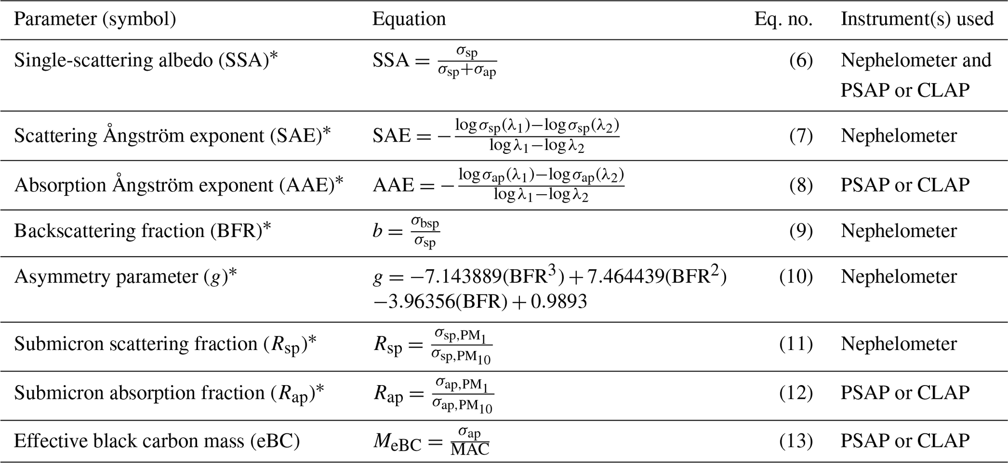
^∗ In this work SSA, BFR, R_sp, and R_ap parameters were derived for the 550 nm wavelength. The SAE was derived using the 450 and 550 nm wavelength data, and the AAE was derived using the 450 and 700 nm wavelength data.

In addition, an effective black carbon mass concentration (M_eBC) was calculated from the PSAP's measured absorption coefficient (σ_ap). This is referred to as an effective mass concentration because its calculation requires the assumptions that (1) all of the measured absorption is from black carbon and (2) all black carbon particles have uniform light absorption efficiencies. This calculation also requires assuming a value for the mass absorption cross section (MAC); frequently, 10 m² g⁻¹ is used. Bond and Bergstrom (2006) suggest that a MAC of 10 m² g⁻¹ is too high for freshly emitted light absorbing carbon, and through the synthesis of available measurements, they suggest an average MAC value of 7.5 ± 1.2 m² g⁻¹ for these aerosols. However, Bond and Bergstrom (2006) acknowledge that ambient and aged aerosol may have larger MAC values. For this work, the MAC of 10 m² g⁻¹ was used, while recognizing that this could be an overestimate.

2.6 Positive matrix factorization analysis

To identify source groupings and contributions at THD, positive matrix factorization (PMF) was used through a consideration of the measured ion component masses and the calculated M_eBC. This study used PMF 5.0, as provided by the United States Environmental Protection Agency (Norris et al., 2014). PMF is a multivariate factor analysis method based on a weighted least squares fit, which was first developed by Paatero and Tapper (1993). The method is a receptor model which solves the chemical mass balance between measured species and source profiles, as shown in the equation below (Norris et al., 2014):

$$\begin{array}{}\text{(14)}& x_{ij}=\sum _{k=\mathrm{1}}^p{g}_{ik}{f}_{kj}+e_{ij},\end{array}$$

where x_ij is the concentration of available species (i is the sample number and j is the number of species), p is the number of factors believed to contribute to the concentrations, g_ik is the relative contribution of the kth factor to the ith sample, f_kj is the concentration of the jth species in the kth factor, and e_ij is the residual value for the jth species.

PMF operates under the constraint that none of the samples can have significantly negative source contributions and derives factor contributions and profiles by minimizing the objective function Q as follows (Paatero and Tapper, 1994; Paatero, 1997):

$$\begin{array}{}\text{(15)}& Q=\sum _{i=\mathrm{1}}^n\sum _{j=\mathrm{1}}^m{\left[{\displaystyle \frac{(x_{ij}-{\sum }_{k=\mathrm{1}}^p{g}_{ik}{f}_{kj}}{u_{ij}}}\right]}^{\mathrm{2}}.\end{array}$$

Here u_ij is the associated uncertainty for the sample x_ij. The associated errors for ion masses were calculated based on the uncertainty analysis provided by Quinn et al. (2000). Any species that were marked as weak in the analysis had an additional 3 % error applied. Since there was a large fraction of unidentified mass in the filter samples (Sect. 3.1.1), the sum of the identified ion mass and not PM₁ was used as the independent variable and total mass in the PMF model in order to avoid overestimating the factor contributions. The associated error for this mass was derived through the propagation of the individual ion errors.

Three error estimation methods were used to validate the PMF solutions, namely displacement analysis (DISP), bootstrap method (BS), and a combination of the two (BS–DISP). PMF solutions were only accepted and reported (1) if the observed drop in Q for DISP was below 0.1 % and no factor swaps occurred for dQ_max​​​​​​​ = 4, (2) from 100 bootstrap runs if all factors had a mapping of ≥ 90 %, and (3) if the observed drop in Q for BS–DISP was below 0.5 % (Brown et al., 2015; Paatero et al., 2014).

2.7 Humidograph measurements

From April 2002–March 2006, a scanning humidity conditioning system (Sheridan et al., 2001) and second nephelometer were operated in series with the first nephelometer in order to determine the scattering enhancement factor f(RH) as a function of relative humidity (RH). The aerosol exited the first nephelometer, which was operating at low RH (so-called “dry”) conditions into a humidity conditioner and controller that stepped the sample airstream through a humidity scan (humidities optimally ranged from ∼ 40 % to ∼ 90 %) over the course of an hour. The humidified airstream then entered the second “wet” nephelometer, and measurements of total scattering (σ_sp,wet) and backscattering coefficients (σ_sp,wet) as a function of relative humidity were obtained. The humidigraph generated hourly scans of increasing RH, with alternating size cuts every 6 min between April 2002 and May 2004. From May 2004 to March 2006, the humidograph performed a 30 min increasing RH scan on the PM₁₀ size cut and then 30 min decreasing RH scan on the PM₁ size cut, as this allowed better control at the high- and low-RH conditions. The scattering enhancement parameter at RH = 85 % and 550 nm was derived from fitting an equation of the following form:

$$\begin{array}{}\text{(16)}& f(\mathrm{RH},\mathit{\lambda })={\displaystyle \frac{{\mathit{\sigma }}_{\mathrm{sp}}(\mathrm{RH},\mathit{\lambda })}{{\mathit{\sigma }}_{\mathrm{sp}}({\mathrm{RH}}_{\mathrm{dry}},\mathit{\lambda })}}.\end{array}$$

We used the THD f(RH) dataset (Burgos et al., 2019b), and further details about the data processing to calculate f(RH) are described in the original publication (Burgos et al., 2019a). The value of f(RH) presented here is the fitted value for wet scattering at 85 % and dry scattering measured at the RH of the dry nephelometer (Table 2). The dry nephelometer RH ranged from ∼ 20 % in the winter to ∼ 40 % in the summer, with an annual median dry nephelometer RH value of 29 %.

2.8 Meteorology

From 2002–2007 the only meteorological parameters measured were wind direction (WD) and wind speed (WS) at 10 m. In 2007, a suite of meteorological measurements was added to the site, including ambient temperature at 2 and 10 m, relative humidity at 2 m, and pressure at 2 m, as well as an additional anemometer for wind direction and speed at 10 m. A 4-year period of overlapping 10 m WD and WS measurements indicated good agreement between the original and new anemometer, and the original anemometer was removed in 2011. Unfortunately, the RH measurements initiated in 2007 were determined to be invalid between 2007–2012 due to the problematic wiring of the sensor, so valid ambient RH data are only available for 2013–2017.

Typical wind directions were the same in summer and winter, but summer tended to be more influenced by flow from the ocean (the northwest). In contrast, in the winter, the wind was more likely to come from the land to the south and east of the site. The diurnal flow regimes indicated in Fig. S3 are consistent with typical onshore–offshore flow observed at many coastal sites. The southeasterly airflow pattern is a land breeze (flowing from land to ocean); it occurs primarily at nighttime (20:00–8:00 PST​​​​​​​) and is directionally consistent with the air coming from nearby coastal communities and the local harbors. In contrast, the northwesterly flow occurs during the day, with the wind coming primarily from the Pacific Ocean. The wind rarely comes from the northeastern sector or the southwestern sector. It should be noted that due to the complex topography near the site, the local wind direction likely represents very local flow patterns. Monthly and diurnal statistical plots of wind data are included in the Supplement (Sect. S2).

3 Results and discussion

3.1 Aerosol chemical components

3.1.1 Seasonal cycles of ionic components

Seasonal median PM₁₀ concentrations for 2002 to 2006 suggest that the ions most likely to be associated with sea salt (i.e., Na⁺, Cl⁻, Mg²⁺, Ca²⁺, K⁺, and Br⁻) are lower in the July–September time period and higher November through April (Fig. 2). This may be due in part to the lower wind speeds in the summer generating less sea spray. PM₁ ions whose primary source is likely to be sea salt (Na⁺, Cl⁻, Mg²⁺, and Ca²⁺) exhibit broadly similar seasonal cycles to those observed for the PM₁₀ measurements, but there are differences in PM₁ and PM₁₀ seasonality for other ions (Fig. 2). PM₁₀ ions associated with marine biogenic activity (MSA⁻ and oxalate) peak in the summer. The PM₁ seasonal cycles for MSA⁻, NH${}_{\mathrm{4}}^{+}$, and SO${}_{\mathrm{4}}^{\mathrm{2}-}$ are similar and peak in May–September, presumably due to marine biogenic activity. However, PM₁ oxalate exhibits relatively stable concentrations throughout the year. This indicates that PM₁ oxalate may come from multiple sources at different times, including biogenic, combustion, and anthropogenic sources (Rinaldi et al., 2011; Saarnio et al., 2010; Andreae, 1983; Baudet et al., 1990; Gao et al., 2003). PM₁ total mass, NO³⁻, and K⁺ concentrations peak in the cooler months (October–January) suggesting that these are likely related to anthropogenic activity (i.e., wintertime residential heating). Comparisons between the PM₁₀ and PM₁ ion concentrations show that MSA⁻, NH${}_{\mathrm{4}}^{+}$, SO${}_{\mathrm{4}}^{\mathrm{2}-}$, and oxalate occur primarily in the PM₁ size range; their concentrations are often extremely close to the median PM₁₀ ion concentrations. Other measured ions, such as, Na⁺, Cl⁻, Mg²⁺, and NO³⁻ are primarily in the supermicron size range; the PM₁₀ concentrations of these ions are at least an order of magnitude higher than their PM₁ concentrations, suggesting a link to sea salt.

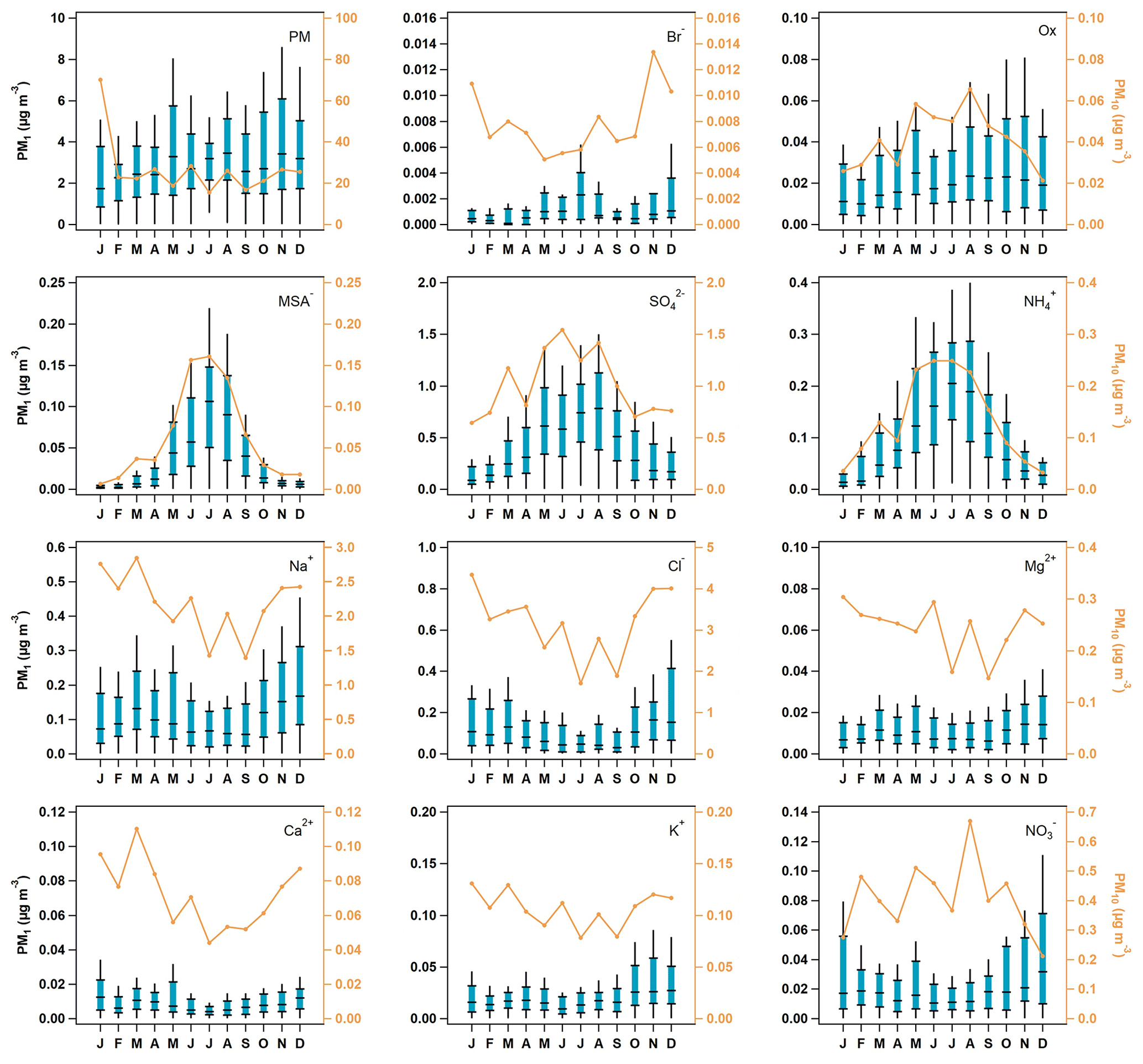
Figure 2 Seasonal aerosol mass and ion concentrations. The blue box-and-whisker plots represent PM₁ aerosol percentiles (5th, 25th, median, 75th, and 95th), and the orange line represents the median concentration of PM₁₀ particles. The PM₁ data scale is on the left axis, while the PM₁₀ is on the right, which has been color-matched to the PM₁₀ trace.

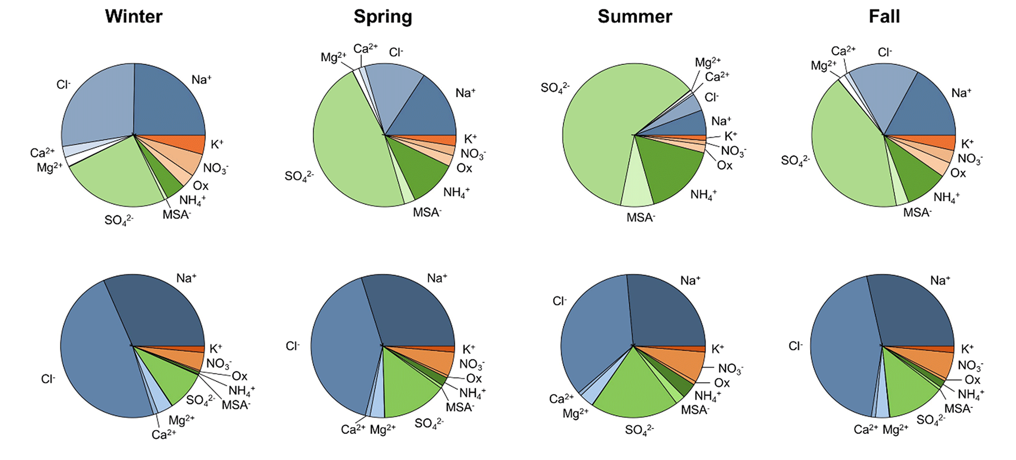
Figure 3 Ion mass fractions for PM₁ (top row) and PM₁₀ (bottom row) in all four seasons. These data are based on total ion mass and not total PM₁ or PM₁₀ mass. Undetermined mass is not included.

For both size fractions, the undetermined mass (which could be organics, insoluble ions, etc.) makes up between 60 %–80 % of the total mass throughout the year (Tables S1 and S2). The estimated contribution of black carbon is discussed later (Sect. 3.1.3). There is no obvious seasonal cycle in the undetermined mass fraction; however, there is seasonality in the fractional contribution of different ions to total ion mass (Fig. 3). Sea salt ions (Na⁺, Cl⁻, Mg²⁺, and Ca²⁺) make up the majority of PM₁₀ ion mass in all four seasons; however, they only dominate the PM₁ ion mass in the winter. In the spring, summer, and fall SO${}_{\mathrm{4}}^{\mathrm{2}-}$ make up the largest fraction of PM₁ ion mass. Both the PM₁ and PM₁₀ ion mass fractions of MSA⁻ are highest in the summer when marine biogenic activity increases. PM₁ fractions of K⁺, NO³⁻, and oxalate are highest in the winter and lowest in the summer; however, the PM₁₀ fraction of K⁺ is relatively consistent across all seasons, and PM₁₀ fractions of NO³⁻ and oxalate are highest in the summer and lowest in the winter.

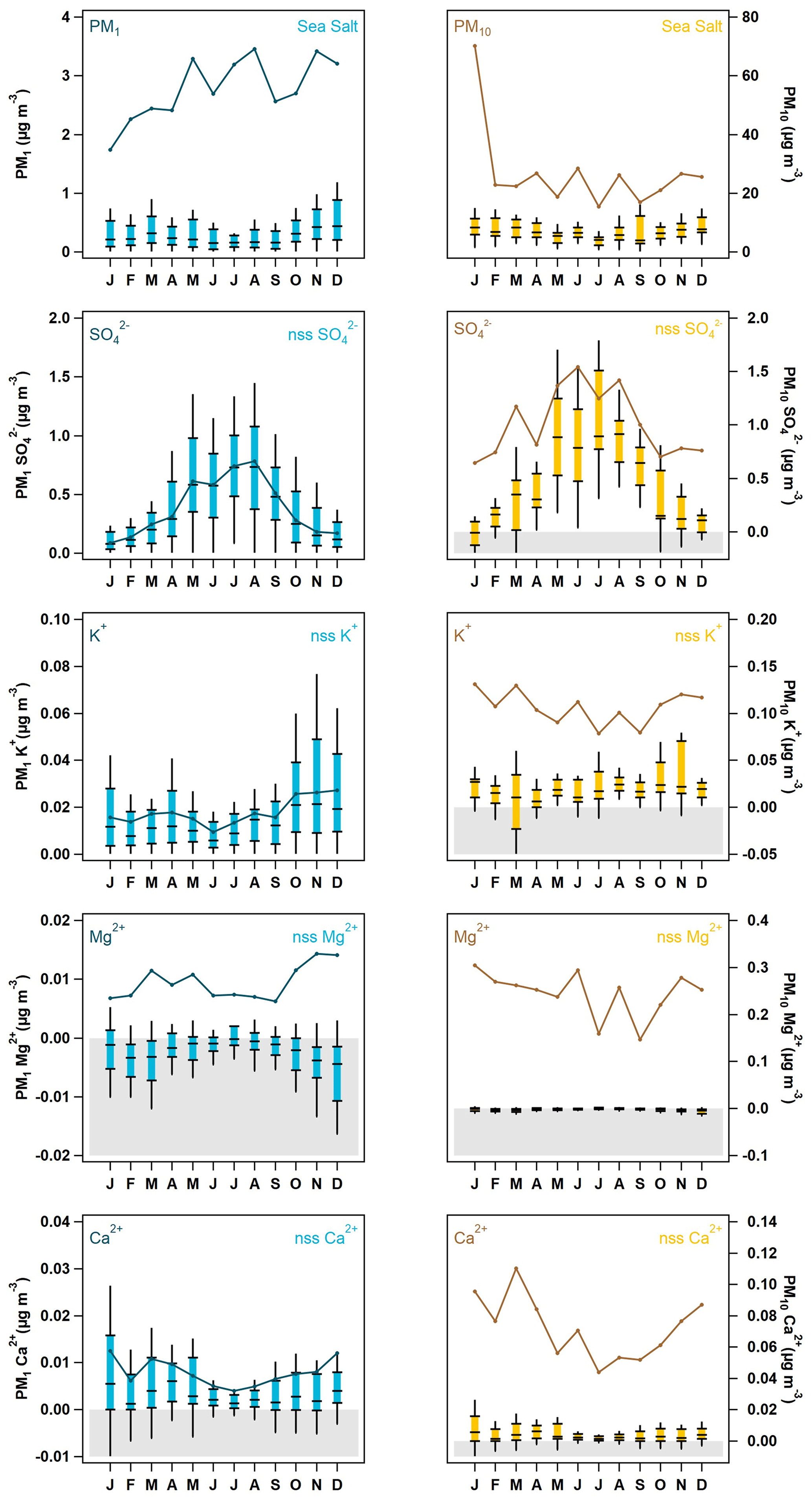
Figure 4 Seasonal cycle of PM₁ (blue) and PM₁₀ (yellow) sea salt and ions with non-sea salt (nss) contributions. The box-and-whisker plots represent the sea salt and nss ion statistics (5th, 25th, median, 75th, and 95th percentiles), while the darker solid line shows the median total measured mass of the ion relative to the sea salt or nss component over the 4-year period. Concentrations that were calculated to be below zero are highlighted in gray in all plots.

Since THD is a marine site, the aerosol chemistry will exhibit a strong sea salt component. It is therefore useful to elucidate the contributions of non-sea salt (nss) ion concentrations relative to those derived from marine sources. The relationships (Eqs. 1–5) from Virkkula et al. (2006) were used to calculate concentrations of sea salt and non-sea salt (nss) ion concentrations, using Na⁺ as the reference species (Sect. 2.2). The estimated seasonal cycle of total concentrations for sea salt and contributions of nss SO${}_{\mathrm{4}}^{\mathrm{2}-}$, K⁺, Mg²⁺, and Ca²⁺ to the total measured concentrations for both PM₁ and PM₁₀ are shown in Fig. 4. Sea salt (due to soluble ions) makes up approximately 30 % of the identified PM₁₀ mass concentration throughout the year but only 5 %–14 % of the PM₁ mass concentration. The lowest sea salt contributions to PM₁ occur from May to September, with higher sea salt contributions during the rest of the year. Virtually all of the PM₁₀ K⁺, Mg²⁺, and Ca²⁺ values are attributable to sea salt (by default, Na⁺ and Cl⁻ are assumed to be solely due to sea salt). Interestingly, the PM₁₀ SO${}_{\mathrm{4}}^{\mathrm{2}-}$ was largely attributable to sea salt in the colder months (November–April); however, from May to October, the nss SO${}_{\mathrm{4}}^{\mathrm{2}-}$ fraction dominated the PM₁₀ SO${}_{\mathrm{4}}^{\mathrm{2}-}$ total concentration. This pattern is consistent with increased biogenic activity in the summer being a source of SO${}_{\mathrm{4}}^{\mathrm{2}-}$. Similar to PM₁₀, PM₁ Mg²⁺ can be almost entirely attributed to sea salt. In contrast, PM₁, SO${}_{\mathrm{4}}^{\mathrm{2}-}$ and K⁺ appear to be primarily nss in origin, while PM₁ Ca²⁺ is marginally attributable to both sea salt and nss sources.

3.1.2 Seasonal ionic relationships as source indicators

We further explored the seasonal relationships between all measured ions using a simple linear regression analysis. Following the ion mass fractions, in the winter, the PM₁ total mass has strong correlations (r > 0.8) with ions likely to be from sea salt (Na⁺, Cl⁻, Mg²⁺, K⁺, and Ca²⁺), whereas in the summer, PM₁ has the strongest correlations with ions associated with biogenic activity (SO${}_{\mathrm{4}}^{\mathrm{2}-}$, MSA⁻, and oxalate). Sodium (Na⁺), magnesium (Mg²⁺), and chloride (Cl⁻) are always highly correlated (r > 0.8), and all three ions have significant relationships (r > 0.5) with calcium (Ca²⁺) in all four seasons. Both Na⁺ and Mg²⁺ correlate with potassium (K⁺) in the winter, spring, and fall; however, Cl⁻ only has significant relationships with K⁺ in the winter and fall. Sulfate (SO${}_{\mathrm{4}}^{\mathrm{2}-}$) is always significantly correlated with methanesulfonic acid (MSA⁻) and oxalate. However, MSA⁻ and oxalate only have strong linear relationships in the winter and summer. Additionally, SO${}_{\mathrm{4}}^{\mathrm{2}-}$ is highly correlated (r > 0.9) with ammonium (NH${}_{\mathrm{4}}^{+}$) in every season, indicating that particles in the area are largely composed of acidic compounds, which is consistent with results presented by Allan et al. (2004), who observed a large particulate sulfate to ammonium ratio in the spring of 2002. Ions that are also associated with anthropogenic emissions (K⁺, nitrate (NO³⁻), and oxalate) are consistently correlated in the winter and fall. K⁺ and oxalate also have a significant relationship in the spring, and the two ions both correlate with NO³⁻ in the summer. The correlation coefficients for all PM₁ ion relationships are listed in the Supplement (Table S3).

The PM₁₀ data exhibit fewer significant relationships between ions, which could be the result of a reduced number of available data points due to weekly sampling. However, there are still clear relationships present. Just as with the PM₁ data, Na⁺, Mg²⁺, and Cl⁻ were always highly correlated (r > 0.8), and all three ions had significant relationships (r > 0.5) with Ca²⁺ in the spring, summer, and fall. Relationships between Na⁺, Mg²⁺, Cl⁻, and K⁺ were the most significant (r > 0.8) in the winter and fall. PM₁₀ SO${}_{\mathrm{4}}^{\mathrm{2}-}$ is highly correlated (r > 0.8) with sea salt ions (Na⁺, Cl⁻, Mg²⁺, and K⁺) in the winter and in the other months is more consistently correlated with NH${}_{\mathrm{4}}^{+}$, NO³⁻, MSA⁻, and oxalate. This is consistent with our nss fraction analysis of SO${}_{\mathrm{4}}^{\mathrm{2}-}$, which showed higher fractions of sea salt SO${}_{\mathrm{4}}^{\mathrm{2}-}$ in the winter months and lower fractions in other seasons. The correlation coefficients for all PM₁₀ ion relationships are listed in the Supplement (Table S4).

From these relationships, there are clear seasonal source groupings of sea salt ions, biogenic ions, and anthropogenic ions. These patterns are further supported by changes in ion concentration ratios across seasons. For instance, the magnitude of the MSA⁻ to nss SO${}_{\mathrm{4}}^{\mathrm{2}-}$ mass concentration ratio can be used to discriminate between the presence of clean marine air with enhanced biological activity when the ratio is high and the existence of anthropogenic sulfate when the ratio is low (Savoie and Prospero, 1989). The PM₁ MSA⁻ $/$ nss SO${}_{\mathrm{4}}^{\mathrm{2}-}$ ratio at THD is highest in the summer, with median values ranging from 0.1–0.15 (equivalent to molar ratios of 8 %–12 %), and lowest in the winter, with median values of 0.02–0.03 that are nearly an order of magnitude lower than the summer ratios (Fig. S4). This generally agrees with the average PM₁ MSA⁻ $/$ nss SO${}_{\mathrm{4}}^{\mathrm{2}-}$ ratio of 0.17 found by Millet et al. (2004) in the springtime period of the NOAA ITCT 2K2 study. Similarly, the mass concentration ratio of oxalate to nss SO${}_{\mathrm{4}}^{\mathrm{2}-}$ can provide evidence for clean marine air or air masses influenced by biomass burning. Zhou et al. (2017) reported oxalate-to-nss-SO${}_{\mathrm{4}}^{\mathrm{2}-}$ ratios of < 0.04 for clean air masses and ratios between 0.1–0.3 for biomass-burning-influenced air. At THD, the PM₁ oxalate $/$ nss SO${}_{\mathrm{4}}^{\mathrm{2}-}$ ratio is lowest in the summer (0.03–0.04) and highest in the winter (0.1–0.15). This pattern is also observable in the PM₁₀ ion ratios; however, there is larger variability (Fig. S4). These ratio values are further evidence of increases in biogenic sources at THD during the summer and increased influences from wood burning for home heating in the winter (City of Arcata, 2008).

3.1.3 Effective black carbon mass contribution

An effective black carbon mass concentration (M_eBC) was calculated for the data using the absorption coefficient (σ_ap) measured by the PSAP. Following the seasonal cycle in absorption (Sect. 3.2), M_eBC was highest in the colder months (September through February) and lowest in the summer (Fig. S6a). M_eBC also exhibited a distinct bimodal diurnal cycle (Fig. S6b), indicating regular sources in the mornings and evenings, which is likely from vehicular and/or maritime traffic. These seasonal observations are discussed further below (Sect. 3.2). For PM₁, M_eBC accounted for 1 %–2.5 % of the total mass, with larger fractions in the winter and fall (Table S1). In contrast, the contribution of M_eBC to PM₁₀ was negligible (> 0.5 %) in all seasons (Table S2).

A linear regression analysis of M_eBC against the other ions in both size fractions was done for the seasonal and monthly data. When grouped by season, PM₁ M_eBC only correlated with oxalate in the winter; however, segregating the data by month showed more relationships of interest. M_eBC correlated with PM₁, SO${}_{\mathrm{4}}^{\mathrm{2}-}$, K⁺, NO³⁻, and oxalate in December and, surprisingly, also had a significant relationship with MSA⁻ during this time. The correlations with SO${}_{\mathrm{4}}^{\mathrm{2}-}$, K⁺, and oxalate were also present in January, and other significant correlations appeared for K⁺ and oxalate in other months (Table S5). For both SO${}_{\mathrm{4}}^{\mathrm{2}-}$ and K⁺, the correlation with M_eBC generally increased when only the non-sea-salt (nss) fraction of the ion concentrations was considered (Table S5). Similar patterns were observed in the PM₁₀ data (Table S6), with significant correlations between M_eBC and PM₁₀, SO${}_{\mathrm{4}}^{\mathrm{2}-}$, K⁺, NO³⁻, MSA⁻, and oxalate being most common in the October–February period. Winter and fall correlations with both SO${}_{\mathrm{4}}^{\mathrm{2}-}$ and K⁺ were again much improved when only the nss fractions were considered. These relationships provide further evidence for the presence of anthropogenic combustion sources in the winter and fall, which aligns with the ion seasonal cycles and correlations discussed previously.

3.1.4 Source identification using PMF analysis

To confirm the ionic source groupings indicated by the linear relationships described above, positive matrix factorization (PMF) was used (Norris et al., 2014). PMF analysis on the entire PM₁ ion dataset, without segregation by season, resulted in the identification of only two factors, based on the quality control criteria used (Sect. 2.3). However, separating the data by seasons resulted in a better resolution of source factors. It should be noted that this seasonal separation did lead to different weighting of ionic compounds among seasons, which is summarized in the Supplement, along with results of the PMF error analysis for each season (Sect. S4). Factor analysis (using an alternative method to the PMF analysis presented here) was performed previously by Millet et al. (2004) on hourly volatile organic compound (VOC) measurements collected at THD during the NOAA ITCT 2K2 study (19 April–22 May 2002). Within the higher-resolution ITCT springtime data, five factors were identified, namely (1) local anthropogenic emissions predominately from fossil fuel use, (2) oxygenated compounds from a variety of sources, (3) long-lived anthropogenic emissions, (4) compounds affected by local atmospheric mixing, and (5) local terrestrial biogenic emissions. Both factors (1) and (4) were strongly influenced by local meteorology, indicating that loss of this resolution could be limiting our factor identification here. While PMF analysis was performed for each seasonal dataset, both the spring (March–May) and fall (September–November) data resulted in two-factor solutions that could not be validated based on subsequent error analysis and are therefore not included in the discussion here.

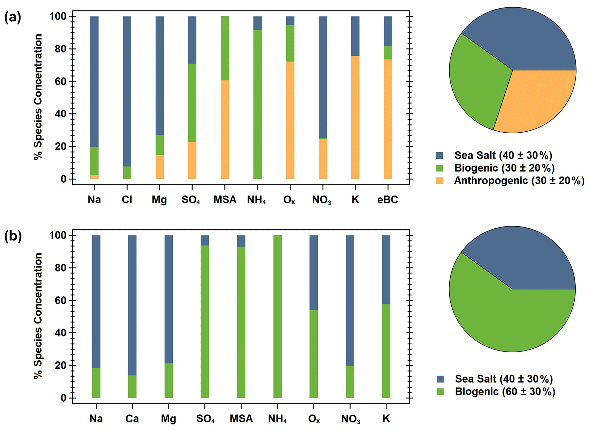
Figure 5 PMF factor information for the (a) winter and (b) summer. The bar charts show the ion species percent contribution to each factor (sea salt is blue, biogenic is green, and anthropogenic is orange), and the pie charts show the percent contribution (listed in the figure legends) of each factor to the seasonal PM₁ mass.

Good correlations were observed between the predicted and observed total identified ion mass for the winter ($y=\mathrm{0.966}x-\mathrm{0.02}$; r² = 0.931; Fig. S7a) and the summer ($y=\mathrm{1.05}x-\mathrm{0.07}$; r² = 0.986; Fig. S7b). For the winter (December–February), a three-factor solution was achieved (Fig. 5a). The first factor is determined to be sea salt, given the high contribution of Na⁺, Mg²⁺, and Cl⁻. The second factor appears to be biogenic, with significant contributions from SO${}_{\mathrm{4}}^{\mathrm{2}-}$, MSA⁻, and NH${}_{\mathrm{4}}^{+}$, along with a small fraction of oxalate. Finally, the third factor is the anthropogenic combustion source, as shown by the high fractions of oxalate, K⁺, and M_eBC. These factor profiles are consistent with the significant ion relationships identified in the winter. Additionally, the sea salt, biogenic, and anthropogenic–combustion factors were estimated to make up approximately 40 ± 30 %, 30 ± 20 %, and 30 ± 20 %, respectively, of the ion mass throughout the winter (Fig. 5a), which is fairly consistent with our direct ion mass calculations (Fig. 3). PMF analysis of the summer ion data (June–August) resulted in a two-factor solution (Fig. 5b). Similar to the winter, in the summer, the first factor is sea salt, with large contributions from Na⁺, Ca²⁺, and Mg²⁺, while the second factor is biogenic, dominated by contributions from SO${}_{\mathrm{4}}^{\mathrm{2}-}$, MSA⁻, and NH${}_{\mathrm{4}}^{+}$ and a significant contribution from oxalate. Sea salt and biogenic factors made up approximately 40 ± 30 % and 60 ± 30 % of the ion mass in the summer, respectively. These factors are consistent with the summertime linear correlations and generally follow ion mass contributions (Fig. 3)

3.2 Aerosol optical properties

3.2.1 Seasonal cycles of optical properties

Seasonal cycles for the optical parameters are consistent across the 15 years of measurements, although the amount of aerosol (as indicated by scattering and absorption) decreases from the start to end of the measurements. General trends in aerosol optical properties at THD over time are further reported on by Collaud Coen et al. (2020). There is an obvious seasonality for most of the aerosol particle properties (Fig. 6), and the PM₁₀ aerosol exhibits similar seasonal patterns to those observed for the PM₁ data. The amount of aerosol – as represented by number concentrations (CN), light absorption, and light scattering (Fig. 6a, b, c) – is highest in fall and winter (September through January), with October and November having the highest aerosol loading and the summer months (June, July, and August) tending to have the lowest loading. The aerosol is darkest (i.e., single-scattering albedo (SSA) is lowest) in the fall and winter (Fig. 6e). A similarly timed decrease in SSA is noted at other (non-marine) North American sites, where it is attributed to less production and/or a more efficient removal of large, highly scattering particles during early autumn (Sherman et al., 2015).

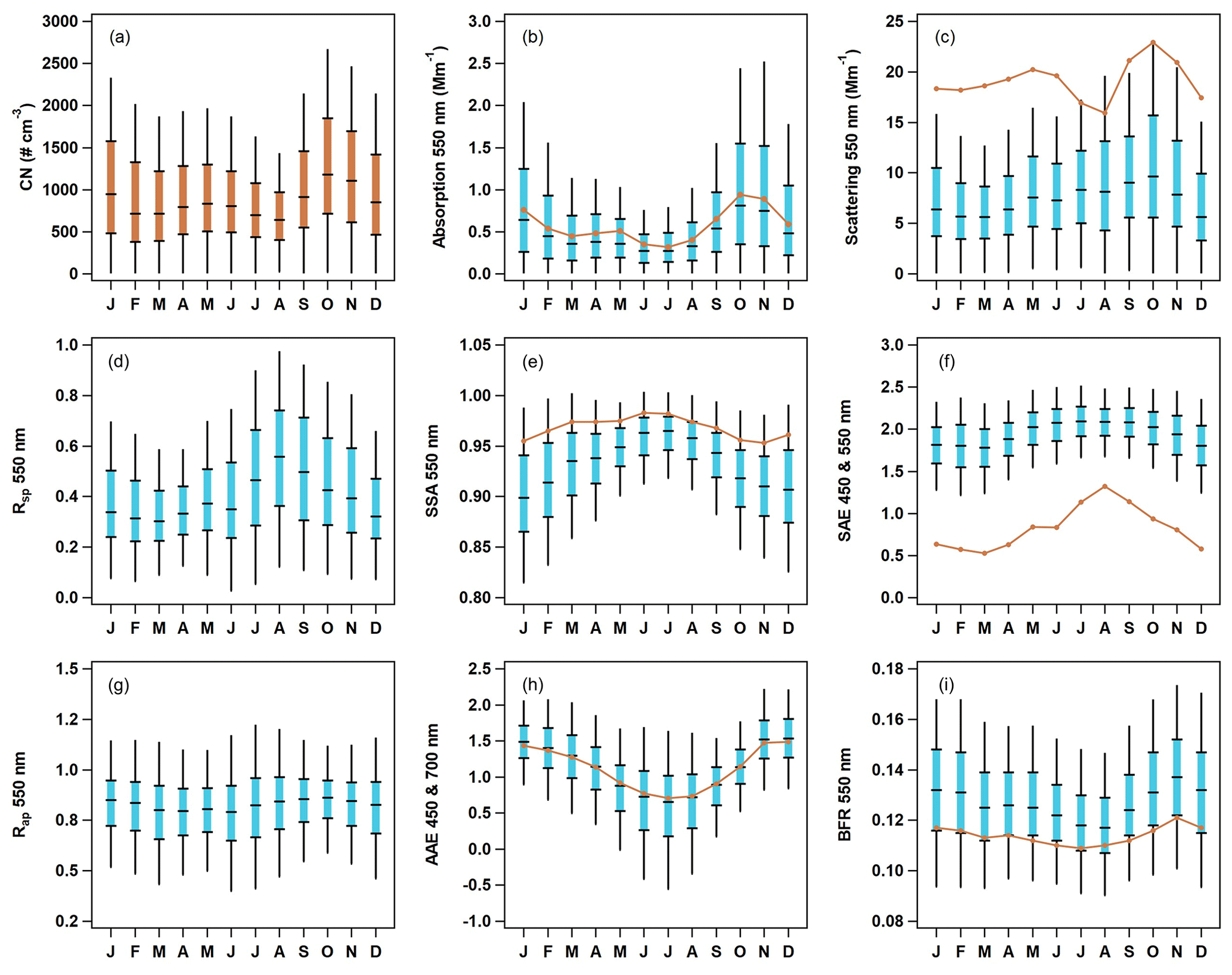
Figure 6 Seasonal cycles of aerosol optical properties at THD. The blue box-and-whisker plots represent PM₁ percentiles (5th, 25th, median, 75th and 95th), and the orange lines represent median values of PM₁₀ optical data. Number concentration data (a) are also in orange, as they include both PM₁ and PM₁₀. The optical parameters presented are (b) absorption at 550 nm, (c) scattering at 550 nm, (d) submicron scattering fraction, (e) single-scattering albedo for 550 nm, (f) scattering Ångström exponent for 450 and 550 nm, (g) submicron absorption fraction, (h) absorption Ångström exponent for 450 and 700 nm, and (i) backscatter fraction at 550 nm.

The seasonality of the aerosol size distribution at THD can be indirectly observed through the monthly cycles in the scattering Ångström exponent (SAE), submicron scattering fraction (R_sp), and the backscatter fraction (BFR). The SAE (Fig. 6f) and submicron scattering fraction (R_sp; Fig. 6d) have similar seasonal patterns. Both SAE and R_sp are highest in summer, indicating a larger contribution from PM₁ particles, and lowest in the winter, demonstrating an increase in large particles. The median values of PM₁₀ SAE (calculated from the 550 and 700 nm wavelength pair) at THD are always below 1.5, and the median values of R_sp are always below 0.6, indicating a significant contribution from supermicron aerosol (likely sea salt) throughout the year. BFR (Fig. 6i) exhibits the opposite pattern of SAE and R_sp; it is lowest in summertime, suggesting a shift toward larger accumulation mode particles in the warmer months. BFR and SAE are sensitive to different parts of the aerosol size distribution (Collaud Coen et al., 2007), so the summertime shift to a higher PM₁ particle contribution (increased SAE) in conjunction with more, larger accumulation-mode particles (decreased BFR) could suggest a narrowing of the size distribution rather than inconsistency in the measurements. In contrast, the lower SAE and higher BFR values in winter could suggest that the size distribution is broader during that time of year. These relationships could also be attributed to changes in the number or relative importance of different aerosol size modes, as multi-modal size distributions can complicate the interpretation of SAE values (Schuster et al., 2006).

Little variation in the submicron absorption fraction (R_ap; Fig. 6g) is observable throughout the year. R_ap values suggests 80 %–90 % of absorption is PM₁ aerosol. In contrast, the absorption Ångström exponent (AAE, as calculated from the 450 and 700 nm wavelength pair; Fig. 6h) exhibits a strong seasonal cycle, with the lowest values (AAE < 1) observed in summer while larger values (AAE ≥ 1.5) are found in winter. AAE values of less than one have been associated with large, non-absorbing particles (Schmeisser et al., 2017), which is consistent with the increased SSA values in the summer, indicating the presence of primarily scattering aerosol (e.g., sea salt). As noted above, PM₁₀ SAE is always less than 1.5, and in general, values of SAE in the summer are elevated, which also supports the presence of smaller non-absorbing aerosols in the summer.

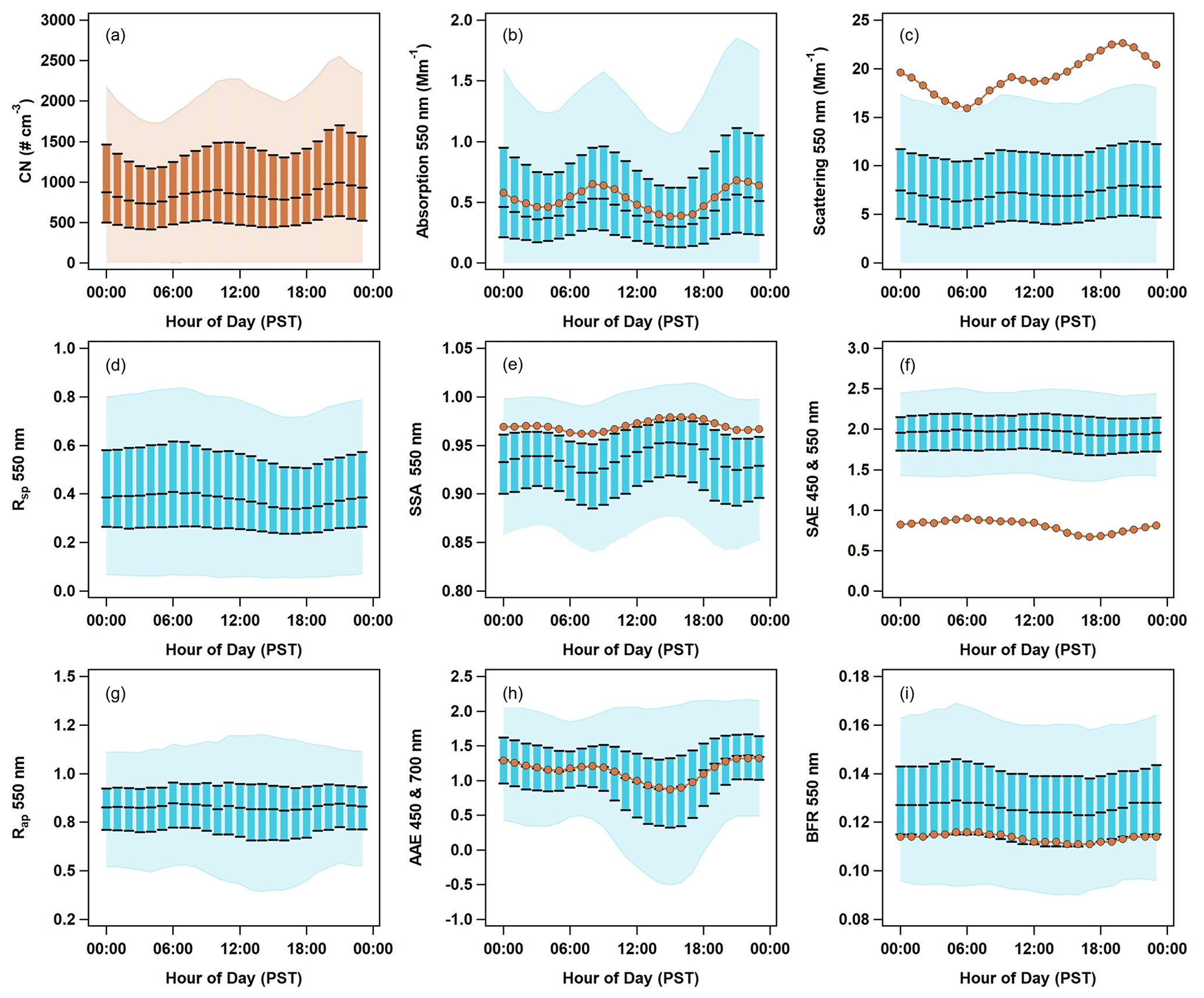
Figure 7 Diurnal cycles of aerosol optical properties at THD. Data are plotted against local time (Pacific standard time). PM₁ optical data are shown in blue, with the light blue shading representing the 5th to 95th percentile, and the blue boxes representing the interquartile range (25th to 75th percentile) and median. PM₁₀ median values are shown as darker orange lines and markers. Number concentration data (a) are also in orange, as they include both PM₁ and PM₁₀. The optical parameters presented are (b) absorption at 550 nm, (c) scattering at 550 nm, (d) submicron scattering fraction, (e) single-scattering albedo for 550 nm, (f) scattering Ångström exponent for 450 and 550 nm, (g) submicron absorption fraction, (h) absorption Ångström exponent for 450 and 700 nm, and (i) backscatter fraction at 550 nm.

3.2.2 Diurnal cycles of optical properties

Two different patterns are observable in the diurnal cycles of aerosol optical property data for all 15 years of sampling at THD (Fig. 7). The first pattern is bimodal, with peaks occurring at ∼ 09:00 and ∼ 21:00 PST. This pattern is most obvious for variables related to aerosol loading (i.e., CN concentration, absorption, and scattering; Fig. 7a, b, c) but is also seen in the diurnal cycles of the single-scattering albedo (SSA; Fig. 7e) and absorption Ångström exponent (AAE; Fig. 7h). The diurnal cycle for SSA has minima coinciding with the aerosol loading maxima. The timing of the diurnal SSA decrease and loading increase suggests a potential anthropogenic–combustion influence, likely vehicular and/or maritime traffic. This bimodal pattern occurs during all seasons, although the timing of the peaks shifts slightly as a function of the season (not shown). The second pattern observed in the diurnal cycle plots is a single broad peak in the morning, with a maximum near 07:00 PST. This broad peak is seen in the plots depicting variables related to particle size (e.g., SAE, R_sp, and BFR; Fig. 7f, d, i). This suggests that smaller particles are most prominent in the early morning (06:00–08:00 PST), as indicated by increases in SAE, R_sp, and BFR at that time. Just like the bimodal cycles discussed earlier, there is some seasonal variation in the timing and amplitude of the broad peak (not shown). For most seasons, the peak occurs at a similar time in the morning, but in the summer, the amplitude of the broad peak is largest and occurs around noon (possibly related to marine biogenic activity). The submicron absorption fraction (R_ap; Fig. 7g) has negligible diurnal variability, suggesting little change in the sources of absorbing aerosol throughout the day.

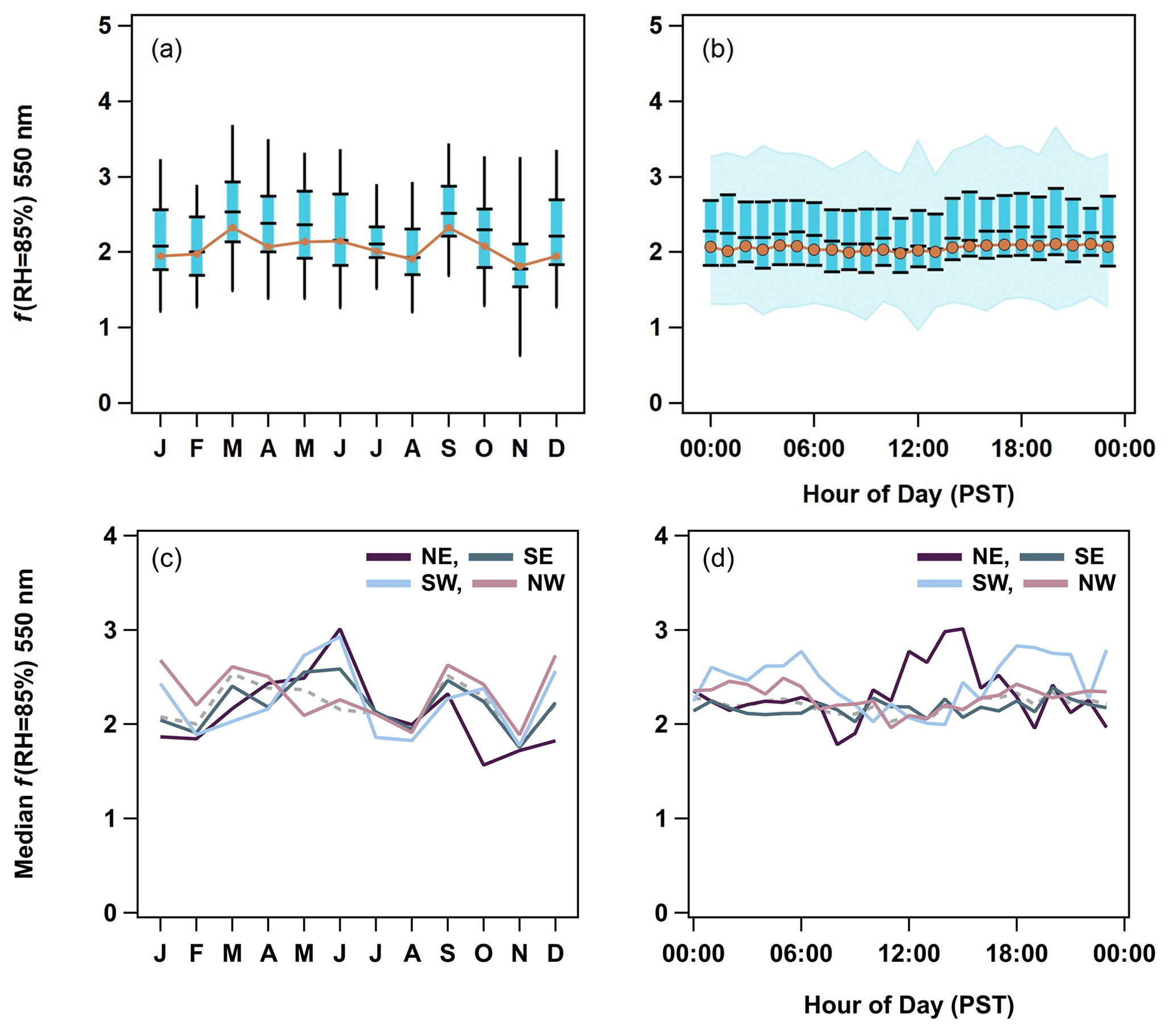
Figure 8 (a) Seasonal and (b) diurnal cycles of f(RH) for 550 nm. The PM₁ 5th to 95th percentiles are indicated by black lines in panel (a) and blue shading in panel (b). The PM₁ 25th to 75th interval is highlighted by blue boxes and black markers. Finally, PM₁ median values are black markers, and PM₁₀ median values are the orange traces. The PM₁ f(RH) cycles are then broken down by wind direction quadrants (northeast (NE), southeast (SE), southwest (SW), and northwest (NW)) on a (c) monthly and (d) hourly basis to show the changes in source regions. The median f(RH) from all of the data is represented as a dashed gray trace in panels (c) and (d).

3.2.3 Temporal cycles in f(RH)

Scattering enhancement parameters (f(RH) = 85 %) are relatively constant throughout the year with a value of ∼ 2. In what follows f(RH) will refer to the enhancement at RH = 85 % unless otherwise stated. The PM₁ f(RH) values are generally higher than those of the PM₁₀ size cut. This is consistent with Zieger et al. (2010), who used Mie calculations to show that, for a given aerosol composition, f(RH) will decrease as the mode diameter of the size distribution increases (their Fig. 9). This is due to the fact that the scattering efficiency factor (Q_scat) is more sensitive to changes in the particle size at smaller diameters where the Mie curve is steeper. At larger particle sizes, the Mie curve is relatively constant. Values for f(RH) observed at THD are also consistent with the literature values of marine aerosol hygroscopicity synthesized in Titos et al. (2016).

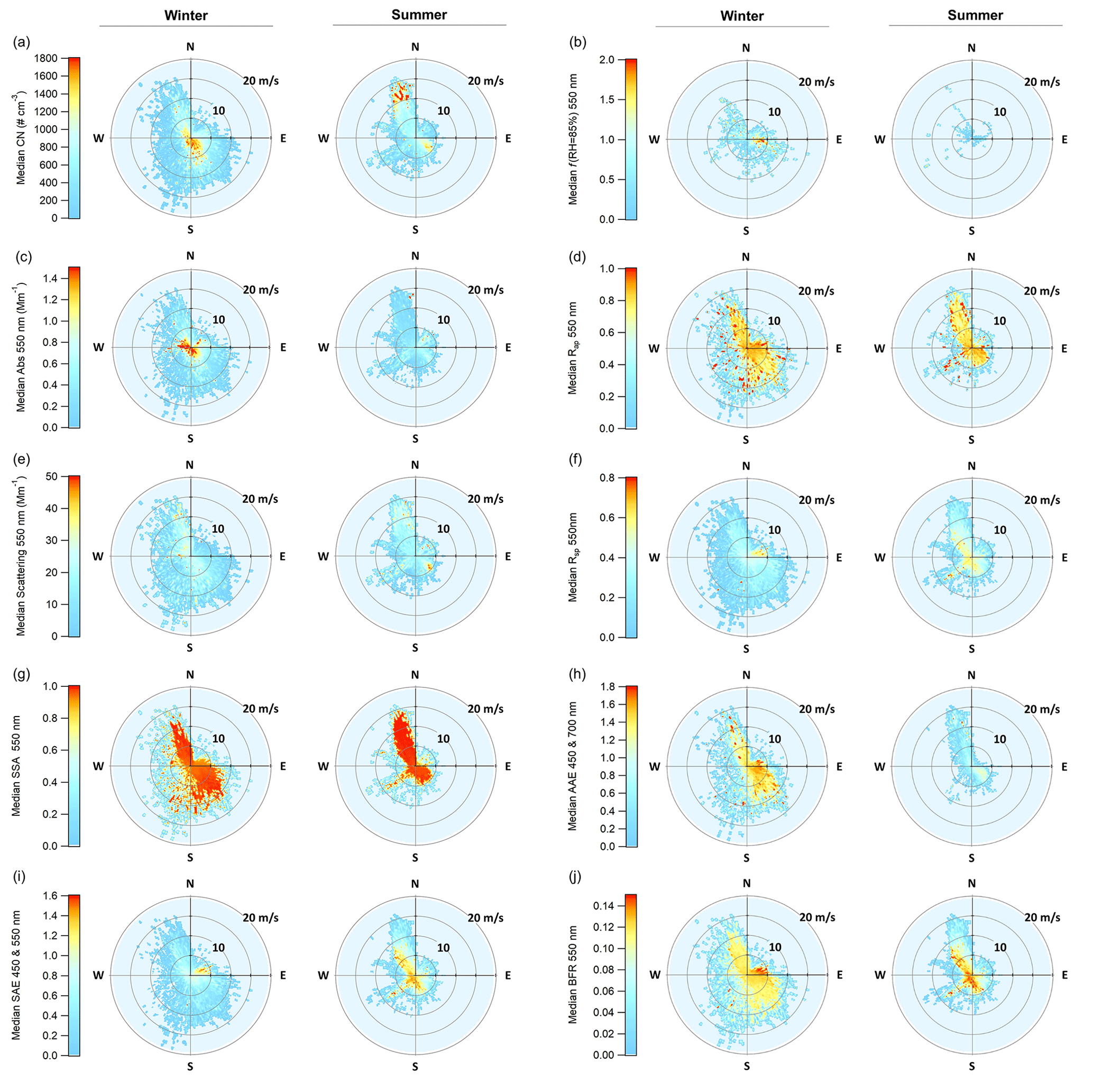
Figure 9 Wind vector analysis for PM₁₀ aerosol optical properties and f(RH = 85 %), showing the median value at a given wind speed and direction. For each property, the winter is on the left and the summer on the right. The color scale on the left applies to both figures.

Surprisingly, neither the average seasonal nor the diurnal cycles in the f(RH) (Fig. 8a, b) reflect the changes in chemistry, particularly the higher levels of SO${}_{\mathrm{4}}^{\mathrm{2}-}$, NH${}_{\mathrm{4}}^{+}$, and MSA⁻ observed in the summer (Figs. 2, 3) and the local anthropogenic sources suggested by diurnal cycles in the optical properties (Fig. 7). Large fractions of sea salt could explain the stability in the PM₁₀ f(RH). This may also, in part, be due to the seasonal cycle of RH values in the dry nephelometer. Zieger et al. (2014) showed that marine aerosol may pick up significant amounts of water at RH values below 40 %. This could result in the seasonal cycle being masked due to the dry aerosol scattering not actually being dry at certain times of year. However, the prevalence of certain wind directions in the dataset clearly affects the overall seasonal cycles in f(RH). Grouping the f(RH) by four major wind quadrants – northeast (0–90^∘), southeast (90–180^∘), southwest (180–270^∘), and northwest (270–360^∘) – allows seasonal and diurnal cycles to emerge (Figs. 8c, d, S8, S9).

Both seasonal and diurnal cycles of PM₁ f(RH) are weakest in the northwestern and southeastern quadrants, which dominated measurements at this site (Figs. S3, S8, S9). The northeastern sector shows patterns that indicate local anthropogenic influences, with f(RH) being lowest in the fall and winter (October–February) and highest in the late spring and early summer (April–June). In the diurnal cycle, there is a decrease in f(RH) at ∼ 08:00 PST, after which the f(RH) steadily increases until ∼ 16:00 PST, which correlates with patterns in the absorption coefficient and other optical properties (Fig. 7). This is evidence for an increase in hygroscopicity as fresh emissions from morning traffic age throughout the day, with the drop in f(RH) later indicating the reintroduction of fresh combustion aerosols from afternoon traffic. These diurnal patterns are weaker but still present in the PM₁₀ data (Figs. S9, S10). Further evidence of anthropogenic sources in the northeast are discussed later (Sect. 3.2.4). The southwestern quadrant has similar seasonal increase in f(RH) in the late spring and early summer (April–June); however, this direction does not exhibit the same decrease in aerosol hygroscopicity in the fall and wintertime. In the diurnal cycle, f(RH) is marginally higher before ∼ 07:00 PST and after ∼ 17:00 PST. This decrease in hygroscopicity could indicate continental influence during the day for winds from this sector; however, this is unlikely, as these decreases do not correlate with decreased SSA or increases in the scattering or absorption Ångström exponent values.

3.2.4 Wind sector analysis of optical properties and f(RH)

To elucidate the impact of different source regions, and subsequent seasonal changes in those sources, PM₁₀ aerosol optical properties were binned both by wind direction and wind speed for summer and winter data (Fig. 9). This wind sector analysis could not be done with the ion mass concentration data because of insufficient time resolution in the data (PM₁ sampled on 24 h intervals and PM₁₀ sampled over week-long periods), which would mask any wind-related information. However, possible changes in composition as a function of wind direction are supported by directional patterns in f(RH) explored previously. Only data after 7 October 2003 were used in this analysis in order to ensure the consistent treatment of the data and remove periods in which wind-direction-based contamination screening process was applied (Sect. 2.2).

Significant differences between optical properties in the summer and winter are apparent in terms of magnitude, distribution across wind sectors, and relation to wind speed. Summertime aerosol number concentration and scattering exhibit more variability across wind directions and speeds but the patterns look quite similar to each other, suggesting a common source (Fig. 9a, e). Both number concentrations and scattering are high when the wind is from the north and relatively strong (∼ 15 m s⁻¹) and also when the wind is from the southeast and the wind speed is low (< 5 m s⁻¹). In the summer, absorption coefficients (Fig. 9c) are highest in air coming from the northeastern quadrant; this peak in absorption only occurs when wind speeds are low (< 5 m s⁻¹), suggesting a local source. In contrast, in the winter, number concentration and absorption cycles (Fig. 9a, c) look similar to each other and both exhibit the highest amount for low wind conditions (i.e., close to the center of each plot), suggesting more local influence and a common source. The highest wintertime scattering comes from the northwest, when wind speeds are high, suggesting increased wind-driven sea spray emissions (Fig. 9e).

Calculated optical properties provide more information about the characteristics of the aerosol in the different sectors. In the winter, there is a clear anthropogenic signal in the northeastern quadrant. Values of SSA are low, while SAE and BFR are both high, suggesting smaller, darker aerosols such as those from combustion sources (Fig. 9g, i, j). This is likely related to home heating from wood burning (City of Arcata, 2008). The low wintertime SSA values correspond with low amounts of scattering in the northeastern quadrant (scattering values are less than 10 Mm⁻¹) and higher amounts of absorption, possibly due to preferential removal of scattering aerosol. Low SAE values also correspond with the lowest observed f(RH) (Fig. 9b), which is consistent with combustion-related aerosol (Maßling et al., 2003; Titos et al., 2016). In the summer, the scattering and the absorption in the northeastern sector both exhibit high values at low wind speeds, and the SSA in the quadrant is generally lower than for the other sectors, again suggesting some sort of local anthropogenic source in that direction. Finally, this temporal cycle is also supported by higher SAE values, indicating a larger contribution of submicron aerosol. It is important to recall that the winds at THD are relatively rare from the northeastern quadrant (∼ 9 % overall; ∼ 7 % in summer and ∼ 14 % in winter; e.g., Fig. S3), so the overall contribution from the quadrant to the aerosol climatology is limited. This was observed previously in the climatology of f(RH) values.

For both summer and winter, SAE values are lower at higher wind speeds (> 10 m s⁻¹), consistent with wind-driven emissions of sea spray (Vaishya et al., 2012). During the summer, the highest SAE values occur during southwesterly flow. This is potentially related to marine biogenic activity, as has been suggested in studies for other marine-influenced sites (Quinn et al., 2002; Yoon et al., 2007) and which is supported by the f(RH) observations for the southwestern quadrant (Sect. 3.2.3). The link between AAE and marine air masses is not clearly defined. For example, Schmeisser et al. (2017) observed that though many of the marine air masses at the sites they studied tended towards lower AAE, no clear pattern could be characterized. The AAE at THD, although exhibiting different values over the seasons, shows a shift from higher AAE in the east (land) to lower AAE in the west (ocean), which generally suggests increased influence from clean marine air (Fig. 9h). This is expected, given the geography of THD.

The relationship between AAE and SAE is thought to be a possible indicator of the type of aerosol being measured (Cappa et al., 2016; Cazorla et al., 2013); however, these regimes have been shown to be less reliable at locations with complex conditions and source types (Schmeisser et al., 2017). In this work, we used the classification scheme from Cappa et al. (2016) to look at general regimes by separating AAE and SAE (450 and 700 nm) comparisons according to both wind direction and season, along with aerosol size, in order to more effectively classify the changes in aerosol types at THD (Fig. S11). PM₁ winter data were largely concentrated in the black carbon (BC)-dominated and BC $/$ brown carbon mixture regions. This shifted down towards the small particle–low absorption region in the spring through fall, with the highest concentration of data in this region during the summer. In all four seasons, the data from the western and eastern quadrants were stratified, with higher ratios for easterly winds (45–135^∘ consistently had the highest ratios of AAE to SAE). Along with the other evidence presented, this supports increased combustion sources in the winter and fall that mainly come from the east, with more biogenic activity in the summer from the west. Comparisons for the PM₁₀ data were similar, although predictably shifted toward larger particle regimes. In contrast to the other seasons, the summer PM₁₀ data from the west remained in the small particle–low absorption group and did not shift into the large particle–low absorption region. Higher R_sp values in the summer support this and point to the formation of small biogenic aerosol during the summer to the west of THD (Fig. 9f).

3.3 Patterns in aerosol composition and optical properties

Aerosol chemical and optical properties have been linked previously at other marine sites. For example, aerosol data from NOAA's Barrow Observatory (Utqiaġvik, AK, USA) exhibited a strong (R² = 0.8) correlation between MSA⁻ and CN concentration during the summer (Quinn et al., 2002), which they attributed to particle formation from biogenic sources. Quinn et al. (2002) also performed linear regressions of aerosol scattering versus derived sea salt and nss SO${}_{\mathrm{4}}^{\mathrm{2}-}$ concentrations at Barrow Observatory and found relatively strong positive correlations (R² > 0.5) for some seasons. At THD, a negligible number of significant relationships (r > 0.5) is observed between ion and CN concentrations; however, several relationships between ion chemistry, scattering, and absorption exist (Tables S9, S10, S11, and S12). Scattering coefficients (σ_sp) correlate with PM₁ mass in the winter and summer. In the summer, σ_sp has a significant relationship with MSA⁻ in July and in August but not in June, indicating the biogenic production of small scattering aerosols in those months. Interestingly, σ_sp correlates with both K⁺ and oxalate in the winter (σ_sp and SO${}_{\mathrm{4}}^{\mathrm{2}-}$ relationships are significant in December and close to significant in January), and the absorption coefficient (σ_ap) correlates with SO${}_{\mathrm{4}}^{\mathrm{2}-}$, K⁺, and oxalate only in the January data. These individual ion to optical relationships are consistent with the PMF analysis discussed previously (Sect. 3.1.4). The PM₁ anthropogenic–combustion factor correlates with the absorption coefficient, indicating that it is driving the increased absorption in the colder months (Fig. S12). While neither the sea salt nor biogenic factors had significant relationships with the scattering coefficient, the biogenic patterns were the stronger (larger r) of the two in both seasons, indicating a stronger impact on scattering (Fig. S12).

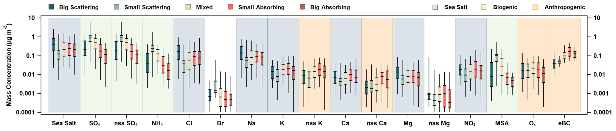
Figure 10 PM₁ ion mass concentrations, together with sea salt and M_eBC, as a function of SSA (550 nm) and SAE (450 and 550 nm). For each species, the mass of big-scattering (SSA > 0.95, SAE < 1.91), small-scattering (SSA > 0.95, SAE > 2.24), mixed (0.89 < SSA < 0.95, 1.91 < SAE < 2.25), small-absorbing (SSA < 0.89, SAE > 2.24), and big-absorbing (SSA < 0.89, SAE < 1.91) aerosol fractions are listed from left to right and color-coded, as outlined in the top-left legend. Additionally, one possible source of the ion based on its distribution across the aerosol types is indicated using shading. Blue shading indicates a sea-salt-related component, green indicates biogenic-related components, and orange indicates anthropogenic–combustion relationships (in the top-right legend).

Another approach to looking at relationships between aerosol chemistry and optical properties is to segment the data by SSA (550 nm) and SAE (450 and 550 nm) and look for differences in mass concentrations for the different groupings of data. This segmentation was done for the PM₁ data (Fig. 10), using the 25th and 75th percentiles of SSA (0.89 and 0.95) and SAE (1.91 and 2.24). Five aerosol groups were defined using the following bounds: big-scattering (SSA > 0.95, SAE < 1.91), small-scattering (SSA > 0.95, SAE > 2.24), mixed (0.89 < SSA < 0.95, 1.91 < SAE < 2.25), small-absorbing (SSA < 0.89, SAE > 2.24), and big-absorbing (SSA < 0.89, SAE < 1.91) aerosols. These group classifications are linked to common aerosol types, such as, marine (big scattering), secondary nucleation (small scattering), anthropogenic (small absorbing), and dust (big absorbing). Bigger, more scattering aerosols had higher concentrations associated with calculated sea salt and its associated ions (Cl⁻, Na⁺, and Mg²⁺), while smaller, more scattering aerosols had higher concentrations of biogenic-related ions (MSA⁻, SO${}_{\mathrm{4}}^{\mathrm{2}-}$ (total and nss fraction), and NH${}_{\mathrm{4}}^{+}$). For darker aerosols, the median for the small-absorbing mass concentration was larger than that of the big-absorbing mass concentration for every species investigated, except Br⁻. Looking at the mass for each of these groups within a given species, patterns in source-related ions and chemical components can be observed (Figs. 10, S13).

3.4 THD as a representative marine site

THD was part of the NOAA Federated Aerosol Network (NFAN), which also includes several clean marine sites at Kennaook / Cape Grim (Australia), Cape Point (South Africa), Samoa (American Samoa), Cape San Juan (Puerto Rico), and Sable Island (Canada; Andrews et al., 2019). Data from these sites compared to that from polluted marine environments show a strong separation between aerosol optical properties (Table 3). Clean marine sites tend to meet the following criteria: σ_sp < 40 Mm⁻¹, σ_ap < 1 Mm⁻¹, SSA > 0.97, and SAE < 1. Anthropogenically impacted sites fail to meet one or more of these constraints. Diurnal variability at clean marine sites is minor, as shown by Delene and Ogren (2002), who reported virtually no diurnal variability in either SSA or BFR at Sable Island (1992–2000), suggesting minimal influence from local sources. THD has diurnal cycles suggestive of anthropogenic influences, similar to those observed by Bhugwant et al. (2001) for absorbing aerosol at a coastal site on Réunion island. However, looking at THD data as a whole, they align most closely with other clean marine sites (Table 3). Comparison to vertical profiles of absorption over the Pacific during the multi-year ATOM (Atmospheric Tomography Mission) campaign can also clarify THD's status as a clean marine site. During ATOM the average mass mixing ratio of refractive black carbon (rBC) in the 20–60^∘ N latitude range over the Pacific Ocean from ATOM was approximately 10 ng kg⁻¹ at the lowest flight level (∼ 0.2 km), which is equivalent to an σ_ap of ∼ 1.2 Mm⁻¹ (assuming dry air mass density of 1.2 kg m⁻³ and MAC 10 m² g⁻¹; Katich et al., 2018). This is well within the range of the aerosol σ_ap measured at THD (Figs. 6, 7), with an annual median σ_ap of 0.62 Mm⁻¹. This leads to the conclusion that, even with influences from local vehicular and marine traffic, seasonal wood burning, and marine biogenic emissions, the majority of measurements made at THD are representative of clean marine air.

Table 3 In situ annual aerosol property statistics at long-term coastal monitoring sites (PM₁₀ or no size cut). Values are reported at the green wavelength (at or near 550 nm) for scattering, absorption, and SSA, unless otherwise noted. Presented SAE values were calculated for a blue or green wavelength pair, unless otherwise indicated (^∗). Values are medians, unless the only available statistic was a mean value.

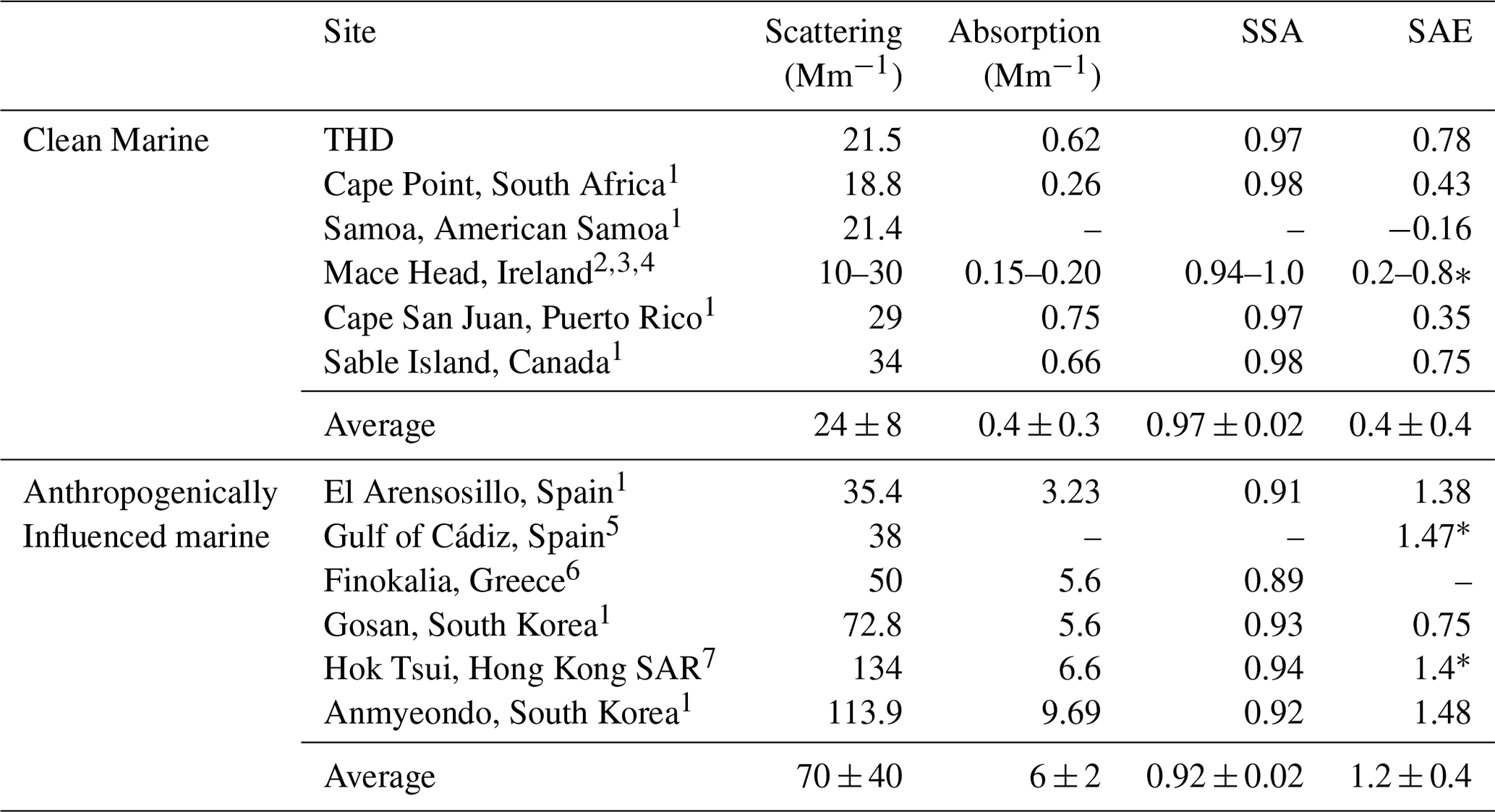
^∗ SAE was measured for the blue and red wavelengths. ¹ Andrews et al. (2019). ² Vaishya et al. (2011). ³ O'Dowd et al. (2012). ⁴ Jennings et al. (2003). ⁵ López et al. (2015). ⁶ Vrekoussis et al. (2005). ⁷ Wang et al. (2017).

4 Conclusions: aerosol sources at THD and THD as a representative marine site

This paper presents the seasonal climatology of aerosol chemical and optical properties from a 15-year dataset obtained at NOAA's now-closed Trinidad Head observatory. As expected, sea salt aerosol is a consistent source at THD and was identified as a source factor in every season (Fig. 5). Calculated sea salt mass, and the mass of its associated ions, consistently dominates PM₁₀ and contributes strongly to PM₁ in the winter (Figs. 2, 3). A consistent PM₁₀ SAE of less than 1.5 and R_sp of less than 0.6 also show the influence of large non-absorbing sea salt throughout the year (Fig. 6). Over all seasons, SAE was lower, and the concentrations of sea salt ions increased at higher wind speeds, indicating wind-driven sea spray emissions that mainly come from the western (ocean-side) quadrants around THD (Fig. 9). Additionally, aerosols at THD are largely composed of acidic compounds, as demonstrated by the relationship between sulfate and ammonium ions in all seasons.

Aerosol ion chemistry and optical properties at THD exhibit monthly and diurnal temporal cycles, suggesting changes in sources, sinks, and transport throughout the year. Biogenic activity contributes to aerosol concentration throughout the year; however, the source is much stronger in the summer (Figs. 2, 3, 5, S4). Large contributions of these small scattering aerosols contribute to both PM₁ and PM₁₀ the summer (Figs. 6, 10, S13). While daily cycles in aerosol optical properties indicate some influence from local traffic emissions (Fig. 7), the winter is the only season with a persistent anthropogenic–combustion source (Figs. 8, 9). This source is only identifiable in the winter (Figs. 5, S4) – likely from wood burning for home heating – and is the driver of increased absorption during this time (Figs. 6, S12). These sources could be further parsed into subcategories; however, this would require higher-resolution chemical data.