Assimilation of POLDER observations to estimate aerosol emissions

We apply a local ensemble transform Kalman smoother (LETKS) in combination with the global aerosol–climate model ECHAM–HAM to estimate aerosol emissions from POLDER-3/PARASOL (POLarization and Directionality of the Earth's Reflectances) observations for the year 2006. We assimilate aerosol optical depth at 550 mnm (AOD₅₅₀), the Ångström exponent at 550 and 865 nm (AE_550–865), and single-scattering albedo at 550 nm (SSA₅₅₀) in order to improve modeled aerosol mass, size and absorption simultaneously. The new global aerosol emissions increase to 1419 Tg yr⁻¹ (+28 %) for dust, 1850 Tg yr⁻¹ (+75 %) for sea salt, 215 Tg yr⁻¹ (+143 %) for organic aerosol and 13.3 Tg yr⁻¹ (+75 %) for black carbon, while the sulfur dioxide emissions increase to 198 Tg yr⁻¹ (+42 %) and the total deposition of sulfates to 293 Tg yr⁻¹ (+39 %). Organic and black carbon emissions are much higher than their prior values from bottom-up inventories, with a stronger increase in biomass burning sources (+193 % and +90 %) than in anthropogenic sources (115 % and 70 %). The evaluation of the experiments with POLDER (assimilated) and AERONET as well as MODIS Dark Target (independent) observations shows a clear improvement compared with the ECHAM–HAM control run. Specifically based on AERONET, the global mean error in AOD₅₅₀ improves from −0.094 to −0.006, while absorption aerosol optical depth at 550 nm (AAOD₅₅₀) improves from −0.009 to −0.004 after the assimilation. A smaller improvement is also observed in the AE_550–865 mean absolute error (from 0.428 to 0.393), with a considerably higher improvement over isolated island sites at the ocean. The new dust emissions are closer to the ensemble median of AEROCOM I, AEROCOM III and CMIP5 as well as some of the previous assimilation studies. The new sea salt emissions have become closer to the reported emissions from previous studies. Indications of a missing fraction of coarse dust and sea salt particles are discussed. The biomass burning changes (based on POLDER) can be used as alternative biomass burning scaling factors for the Global Fire Assimilation System (GFAS) inventory distinctively estimated for organic carbon (2.93) and black carbon (1.90) instead of the recommended scaling of 3.4 (Kaiser et al., 2012). The estimated emissions are highly sensitive to the relative humidity due to aerosol water uptake, especially in the case of sulfates. We found that ECHAM–HAM, like most of the global climate models (GCMs) that participated in AEROCOM and CMIP6, overestimated the relative humidity compared with ERA5 and as a result the water uptake by aerosols, assuming the kappa values are not underestimated. If we use the ERA5 relative humidity, sulfate emissions must be further increased, as modeled sulfate AOD is lowered. Specifically, over East Asia, the lower AOD can be attributed to the underestimated precipitation and the lack of simulated nitrates in the model.

1 Introduction

A prominent uncertain component in aerosol modeling is the aerosol emissions. The uncertainty in aerosol emissions enhances the unpredictability in the simulated aerosol concentration and optical properties (Textor et al., 2007) as well as in the aerosol radiative effect and forcing (Myhre et al., 2013; Yoshioka et al., 2019). A bottom-up estimate of anthropogenic aerosol emissions usually comes from the integration of known sources of information across different economic sectors, such as power, industry, transport and residential (Zhang et al., 2009). These bottom-up techniques are very useful since they provide a first-guess estimate of aerosol emissions, but emission differences in source attribution (power, industry, residential) may lead to very different simulated aerosol concentrations (Saikawa et al., 2017).

Natural aerosol emissions like dust and sea salt are estimated in aerosol models through different schemes by using wind speed as well as land or ocean characteristics (Grythe et al., 2014; Long et al., 2011; Tegen et al., 2002). A large fraction of the natural emissions diversity can be attributed to differences in the modeling approaches. Emission schemes can differ in the parameterization of source strength as a function of wind (Grythe et al., 2014; Textor et al., 2007), the simulated winds themselves (Textor et al., 2007), the simulated size spectrum of the emitted particles (Kok et al., 2021; Textor et al., 2006), the simulated size grouping in each model (e.g., modes or bins) (Gliß et al., 2021) and the implementation of spatial filters where dust emission sources can change dynamically based on vegetation (Wu et al., 2020). Also, large differences in the simulated natural emissions can emerge by simply using a different horizontal resolution in the same model (Guelle et al., 2001; Laurent et al., 2008). In addition, the physically relevant scale (from 1 m to several km) where dust emissions can vary is not captured by the current horizontal resolution of global climate models (Kok et al., 2021).

Emissions from biomass burning are estimated based on satellite measurements that are related to burned area and that use emission factors to convert the burned dry matter into emissions of aerosol and gas species (Global Fire Emissions Database v4 (GFED4); Van der Werf et al., 2017), active fire count (Fire INventory from NCAR v1.5 (FINN1.5); Wiedinmyer et al., 2011), or fire radiative power (Quick Fire Emissions Dataset v2.4 (QFED2.4); Darmenov and da Silva, 2015; Fire Energetics and Emissions Research version v1.0 (FEER1.0); Ichoku and Ellison, 2014; and Global Fire Assimilation System (GFAS); Kaiser et al., 2012). It has been shown that different emission factors may contribute to the diversity between these emission inventories, but differences in the dry matter have also been reported for North America fires (Carter et al., 2020), which is one of the main reasons that the fire detection and/or fire burden area inventories do not align with fire radiative power inventories (Van der Werf et al., 2017). In addition, strong interannual differences and regional diversity are observed between the datasets, with a fairly good agreement over the Amazon and a quite high disagreement over Africa and boreal North America (Carter et al., 2020).

The global dust emissions relative diversity (usually quantified as the ratio of the standard deviation to the mean) (Schutgens et al., 2020) for the multi-model ensemble of CMIP5 is 87 % (Wu et al., 2020), and for AEROCOM I it is 73 % (Huneeus et al., 2011), while for several simulations from a single model with diverse emission scheme settings it is 61 % (Miller et al., 2006). The sea salt emission relative diversity is 97 % based on several different sea salt emission functions (Grythe et al., 2014) for global estimates within the range of 1200 to 20000 Tg yr⁻¹ as proposed by Lewis and Schwartz (2004). The emission relative diversity from biomass burning based on six emission datasets is 76 % for organic carbon and 82 % for black carbon (Pan et al., 2020). Consequently, the global emissions of aerosol from natural sources, such as deserts (dust), oceans (sea salt) and non-anthropogenic biomass burning (organic and black carbon – OC and BC), are at least higher than 60 %; hence there is a lot of room for improvement.

The differences between various anthropogenic emission inventories is considerably lower than the differences between various natural emission estimates for aerosol. In Lee et al. (2013), lower OC and BC uncertainty was found for fossil fuel compared with biomass burning emissions as well as lower SO₂ uncertainty for fossil fuel compared with volcanic emissions. The emission diversity estimated by multiple anthropogenic emission inventories, as the ratio of the highest to the lowest anthropogenic global emissions, showed that it is lower than 20 % for BC and NO_x and lower than 42 % for SO₂ after the year 2000 (Granier et al., 2011). The relative diversity of anthropogenic aerosol and aerosol precursor emissions over large areas is significantly lower, but note that these different emissions inventories are constructed using very similar information and methods; therefore they are not independent from each other (Granier et al., 2011). Based on four emission inventories over eastern China for 2006, the emissions relative diversity (using the mean in the denominator) of SO₂, ammonia (NH₃), OC and BC is 5 %, 18 %, 12 % and 16 %, respectively (Chang et al., 2015). Note that this diversity is based on yearly means; hence the day-to-day variability and relative diversity among these emission inventories can be higher. Further, the sector attribution of emissions can be quite different in each dataset, which can affect the uncertainty in emissions on the regional level (Saikawa et al., 2017).

These high emissions differences for modeled fluxes of dust and sea salt as well as differences in fluxes in emission inventories for the other aerosol species led to the popularization of the top-down method that combines simulated aerosol information from a model and retrieved aerosol information from satellites (Chen et al., 2018, 2019, 2022; Dubovik et al., 2008; Escribano et al., 2017; Huneeus et al., 2012; Jin et al., 2019; Pope et al., 2016; Schutgens et al., 2012; Sekiyama et al., 2010; X. Xu et al., 2013). The simulated aerosol state in the model is produced using background emissions which are either prescribed from emission inventories (anthropogenic aerosols and biomass burning) or interactively calculated through emission schemes (dust and sea salt aerosols). In addition, the uncertainty in the assimilated observations and the uncertainty in the background emissions need to be specified.

Most of the abovementioned studies have estimated new emissions based on the assimilation of aerosol optical depth (AOD), some studies have also included the Ångström exponent (AE), while very few studies have assimilated absorption observations like absorption aerosol optical depth (AAOD) or single-scattering albedo (SSA) (Zhang et al., 2015; Chen et al., 2018, 2019, 2022). By not including observations of measurements related to size and absorption, the estimated emission may be misrepresented as it has been shown for the estimated aerosol mixing ratio in Tsikerdekis et al. (2021), where several data assimilation experiments were conducted with different combinations of observations from the POLDER (POLarization and Directionality of the Earth's Reflectances) instrument. The multi-wavelength and multi-viewing-angle photopolarimetric measurements of POLDER contain more information about the scattered solar radiation compared with single-viewing measurements (Hasekamp and Landgraf, 2007; Mishchenko and Travis, 1997); hence POLDER is an ideal tool for obtaining accurate aerosol microphysical and optical properties, which can potentially provide a more accurate estimation of emissions, as suggested in Schutgens et al. (2021).

Although aerosol emissions are critically uncertain, other factors can affect the uncertainty in modeled aerosol concentration and optical properties. One of these factors is the aerosol water uptake in models that can considerably increase the simulated AOD diversity (Gliß et al., 2021). The misrepresentation of water uptake can have a huge impact, since the condensed water over dry aerosol particles may contribute up to 70 % of the total AOD globally (K. Zhang et al., 2012). During the AEROCOM I phase, substantial diversity among the model was attributed to differences in the modeled water uptake (Kinne et al., 2006). A recent study has evaluated the scattering enhancement factor of 10 Earth system models based on 22 ground-based in situ measurements (Burgos et al., 2020). The scattering enhancement factor for a certain wavelength (λ) is the ratio of the light scattering coefficient under wet (relative humidity (RH) = 85 %) to dry (RH = 40 %) conditions, which describes the increase in aerosol scattering due to the wet growth of particles under different RH conditions. The results showed that the models tend to overestimate the scattering enhancement factor as an ensemble mean by 15 %, though the differences from model to model were quite substantial. The inter-model differences were attributed to different assumptions in kappa and contrasting growth under low-RH (RH < 40 %) conditions between the models. Further, it was suggested that lower kappa values should be used in the models for organics and sea salt, and considerable differences were found between the models for the light scattering enhancement factor under relatively dry conditions (RH < 40 %). Although this study is very insightful, the discretization of the scattering enhancement factor based on RH could correspond to a diverse aerosol load for each model. The low- and high-RH conditions may have occurred at different times and on different dates for every model and for the observations. In our study we assume that kappa is correct for our experiments, and we investigate how a biased RH may influence aerosol water growth and their optical properties as well as estimated aerosol emissions by the data assimilation system.

The effect of a biased RH, which can dramatically affect the simulated aerosol optical properties, has so far received little attention. The current horizontal resolution of global climate models (GCMs), which for the majority of AEROCOM III and CMIP6 models is between 1^∘ and 2^∘ (Gliß et al., 2021; Z. Xu et al., 2021), cannot resolve humidity's small-scale processes; thus they are parameterized through cloud schemes (Lin, 2014). Because of this, biases in the simulated humidity can accumulate in GCMs. The specific humidity of the CMIP5 ensemble is overestimated over midlatitudes throughout the troposphere when compared with the Atmospheric Infrared Sounder (AIRS) (Tian et al., 2013). Further, the majority of the CMIP6 model ensemble (12 out of 18) overestimates relative humidity at 850 hPa in all seasons compared with ERA5 (Z. Xu et al., 2021).

In the present study we estimate the aerosol emissions of dust (DU), sea salt (SS), organic carbon (OC), black carbon (BC), sulfates (SO₄) and precursor gas emissions for sulfates like sulfur dioxide (SO₂) and dimethyl sulfide (DMS) for the year 2006. Our method implements a local ensemble transform Kalman smoother (LETKS), which has been introduced in our preceding work (Tsikerdekis et al., 2022a). It combines POLDER observations, which were retrieved by the algorithm developed at the Netherlands Institute for Space Research (SRON), with the aerosol information simulated by ECHAM–HAM. We assimilate AOD₅₅₀, AE_550–865 and SSA₅₅₀ in order to simultaneously account for the correction of aerosol mass, size and absorption (Tsikerdekis et al., 2021). In addition, we conduct sensitivity and data assimilation experiments using the relative humidity of ERA5 (instead of ECHAM–HAM) for the water uptake process to quantify the effect it has on aerosol optical properties and the estimated emissions. Section 2 presents the retrieved observations from POLDER and the model ECHAM–HAM. The observations and emissions uncertainties are discussed. Section 3 briefly describes the LETKS and provides an overview of our experiments. Section 4 includes the evaluation results of our experiments against POLDER and independent observations (AERONET and MODIS) as well as the new estimated emissions along with the reported emissions from previous studies. In addition, we quantify the effect of a biased high RH on aerosol optical properties and emissions.

2 Data

2.1 Aerosol observations (POLDER)

POLDER-3 (POLarization and Directionality of the Earth's Reflectances) is an instrument that can measure light intensity and polarization properties from up to 16 viewing angles and from multiple wavelengths (0.44 to 1.02 µm). In addition, the multi-angle multi-wavelength photopolarimetric measurements have the ability to differentiate scattering of cloud droplets from aerosol particles; thus the exclusion of cloud-contaminated pixels is possible (Stap et al., 2015). The instrument was part of the Polarization and Anisotropy of Reflectances for Atmospheric Sciences coupled with Observations from a Lidar (PARASOL) micro-satellite, which was active from 2004 to 2013.

The aerosol products derived from POLDER observations that were used in this study were retrieved by an algorithm developed at SRON (Netherlands Institute for Space Research), which fits a radiative transfer model (Hasekamp and Landgraf, 2005; Schepers et al., 2014) to the multi-angle photopolarimetric measurements of POLDER to derive aerosol optical properties corresponding to a bimodal aerosol size distribution. We use the global bimodal product, which is the only product available globally, but note that a regional 10-mode product achieved higher accuracy for AOD and a similar performance for SSA when compared with AERONET for retrievals over land (Fu and Hasekamp, 2018). The retrieved properties for a fine- and coarse-mode particle are the effective radius, the effective variance and the column number concentration as well as the real and imaginary part of the refractive index for each mode (Hasekamp et al., 2011, 2019; Lacagnina et al., 2015; Wu et al., 2015). By using the abovementioned aerosol parameters for the two modes, we can calculate the aerosol optical depth (AOD), the Ångström exponent (AE), the absorption aerosol optical depth (AAOD) and the single-scattering albedo (SSA). The aerosol optical properties of POLDER retrievals demonstrate good agreement with either ground-based (AERONET) or satellite (Ozone Monitoring Instrument; OMI) retrievals for the year 2006 (Hasekamp et al., 2011; Lacagnina et al., 2015, 2017; Stap et al., 2015).

In the present study, aggregated (1^∘ × 1^∘) POLDER data are used in the assimilation for the year 2006. The year 2006 was selected based on the availability of POLDER aerosol products from the SRON retrieval algorithm. POLDER uncertainty for each assimilated observable was estimated for several POLDER AOD₅₅₀ bins based on an AERONET evaluation and is presented in Appendix A. Note that POLDER AE_550–865 over the Sahara is biased high based on AERONET; thus these observations were not assimilated (see Appendix A). A more detailed description of the use of POLDER data in our assimilation system can be found in Tsikerdekis et al. (2021), and details on the SRON POLDER retrieval algorithm can be found in Fu et al. (2020) and Fu and Hasekamp (2018).

2.2 Aerosol model (ECHAM6–HAM2)

The aerosol–climate model ECHAM6–HAM2 (hereafter called ECHAM–HAM) is used to simulate the meteorological and aerosol state of the atmosphere. The model consists of two parts, the general circulation model ECHAM6, developed at the Max Planck Institute for Meteorology (MPI-M) in Hamburg, Germany (Stevens et al., 2013), and the second version of the Hamburg Aerosol Model (HAM2) (Stier et al., 2005; Tegen et al., 2019; K. Zhang et al., 2012). Aerosols are simulated in seven unimodal lognormal particle size distributions (modes); four of them are the hydrophilic nucleation, Aitken, accumulation and coarse, while three of them are the hydrophobic Aitken, accumulation and coarse. Each mode may contain one or more (internally mixed) aerosol species, namely dust (DU), sea salt (SS), organic carbon (OC), black carbon (BC) and sulfates (SO₄) (Vignati et al., 2004). Currently the model does not simulate aerosol nitrates. The cloud and aerosol optical properties are computed using Mie theory and are derived from lookup tables (Tegen et al., 2019) using the prognostic concentrations of aerosol tracers (Schultz et al., 2018).

All aerosol species are emitted, transported and deposited, and they take part in aerosol–radiation interactions (scattering and absorption) as well as in aerosol microphysical processes (e.g., nucleation, coagulation, aerosol water uptake and cloud activation) (Schutgens and Stier, 2014; K. Zhang et al., 2012). The natural aerosol types (DU, SS) are introduced into the atmosphere by utilizing the simulated information of wind and certain surface and ocean characteristics. Other aerosol species (OC, BC) or aerosol precursor gasses (SO₂, DMS) that are emitted from both natural (biomass burning or biogenic emissions) and anthropogenic sources (e.g., industry and transport) use predefined emission inventories (K. Zhang et al., 2012). Specifically, anthropogenic emissions are derived from 14 different sectors. Each sector may include one or more aerosol types or aerosol precursors (Schultz et al., 2018; Tegen et al., 2019). A more detailed description of the model is available in our preceding work (Tsikerdekis et al., 2021, 2022a).

Aerosol water uptake is the process of condensing water vapor on the surface of aerosol particles. This process affects the aerosol's size, deposition, atmospheric lifetime and optical properties. Thus, it is crucial to simulate aerosol water uptake accurately in aerosol models. In ECHAM–HAM water uptake is simulated by a semi-empirical water uptake scheme (O'Donnell et al., 2011) that approximates the enhancement of particle size (growth factor; gf) based on Petters and Kreidenweis (2007). Based on this scheme the growth of aerosol particles depends on the relative humidity (RH); the dry particle radius (Dp); the kappa parameter (κ), which is distinctive for each aerosol species and which determines its hygroscopicity; and the Kelvin term (A), which is a temperature-dependent constant (O'Donnell et al., 2011). In order to enhance computational efficiency, this equation is solved offline and is organized in lookup tables where the aerosol growth factor can be determined for specific RH, Dp, k and A conditions in each grid cell of the model. Kappa expresses the volume of water that is associated with a unit volume of dry particles (Petters and Kreidenweis, 2013), and the higher it gets, the more soluble the aerosol species is. In ECHAM–HAM the kappa is fixed for each species. The kappa specifically for SS, SO₄ and OC is equal to 1.00, 0.60 and 0.06, respectively. DU and BC are considered insoluble (κ=0). The most decisive parameter of the above, which influences the growth factor of soluble particles (high κ) the most, is RH. Hence, in this study we conduct experiments where RH from ERA5 is explicitly used for the water uptake of aerosols in ECHAM–HAM to quantify its effect on the simulated aerosol optical properties. Further, this option is adopted in a data assimilation experiment to quantify the effect of RH on aerosol emission estimation.

3 Methods

3.1 The local ensemble transform Kalman smoother

The local ensemble transform Kalman smoother (LETKS) is used to estimate aerosol emission. This method was previously used by Schutgens et al. (2012) for aerosol emission estimation and earlier for CO₂ emission estimation (Bruhwiler et al., 2005; Peters et al., 2005; and Feng et al., 2009). A detailed description of LETKS can be found in Tsikerdekis et al. (2022) where the method and the code were tested for aerosol emission estimation using SPEXone synthetic measurements in observing system simulation experiments (OSSEs). Here the main components of the method are discussed.

The system estimates perturbation to the background emissions and assumes that these perturbations remain constant over 2 d. The emission perturbations are estimated using assimilation cycles, where each cycle consists of a background and an analysis step. The background step produces the required background information based on an 8 d (ΔT_b) forward simulation of ECHAM–HAM driven by a priori (“background”) emissions. The analysis step assimilates all the available POLDER observations within the last 2 d (ΔT_s) of the forward simulation and estimates the “analysis” emissions for the last 6 d ($\mathrm{\Delta }{T}_{\mathrm{a}}=\mathrm{\Delta }{T}_{\mathrm{b}}-\mathrm{\Delta }{T}_{\mathrm{s}}$) of the forward simulation.

At the end of each assimilation cycle the estimated analysis emissions of the previous cycle serve as background emissions for the next cycle, time is shifted forward equal to ΔT_s days, and the background and analysis steps are repeated. Note that with this setup several assimilation cycles overlap in time; thus the estimated emissions (estimated in batches of 2 d) are affected by observations of the current and subsequent days. Specifically, the emissions of a day may be affected by observations of the same day and of the 5 subsequent days. This iterative design ensures that observations close to the sources along with observations away from the sources (e.g., an aerosol plume created by particles emitted several days earlier) will both be used to correct the emissions.

The assumed background emissions are uncertain. The uncertainty in the emissions is represented with an ensemble of 32 simulations where emissions are perturbed. The perturbation is conducted by multiplying the emissions by spatially correlated perturbations (see Sect. 3.2 on Tsikerdekis et al., 2021). The spatial correlation length scale of the perturbations is approximately 25^∘ omnidirectionally, except for DU perturbations over the Sahara where the spatial correlation length is zero (perturbations from grid to grid are uncorrelated). The zero spatial correlation length for DU over the Sahara was chosen after conducting several data assimilation experiments with different correlation length values and evaluating them in terms of AOD₅₅₀ (not shown). Each perturbation set is uniquely generated for every perturbed parameter and ensemble member. In each grid cell, the mean of the background distribution of the emission scaling factor for the first cycle is equal to 1, while for all subsequent cycles the mean is set equal to the analysis distribution mean of the previous cycle (see prior correction subsection in Tsikerdekis et al., 2022a). In each grid cell, the standard deviation of the background distribution, which represents the uncertainty in the emissions, is distinct for each perturbed parameter and is further discussed in Appendix B.

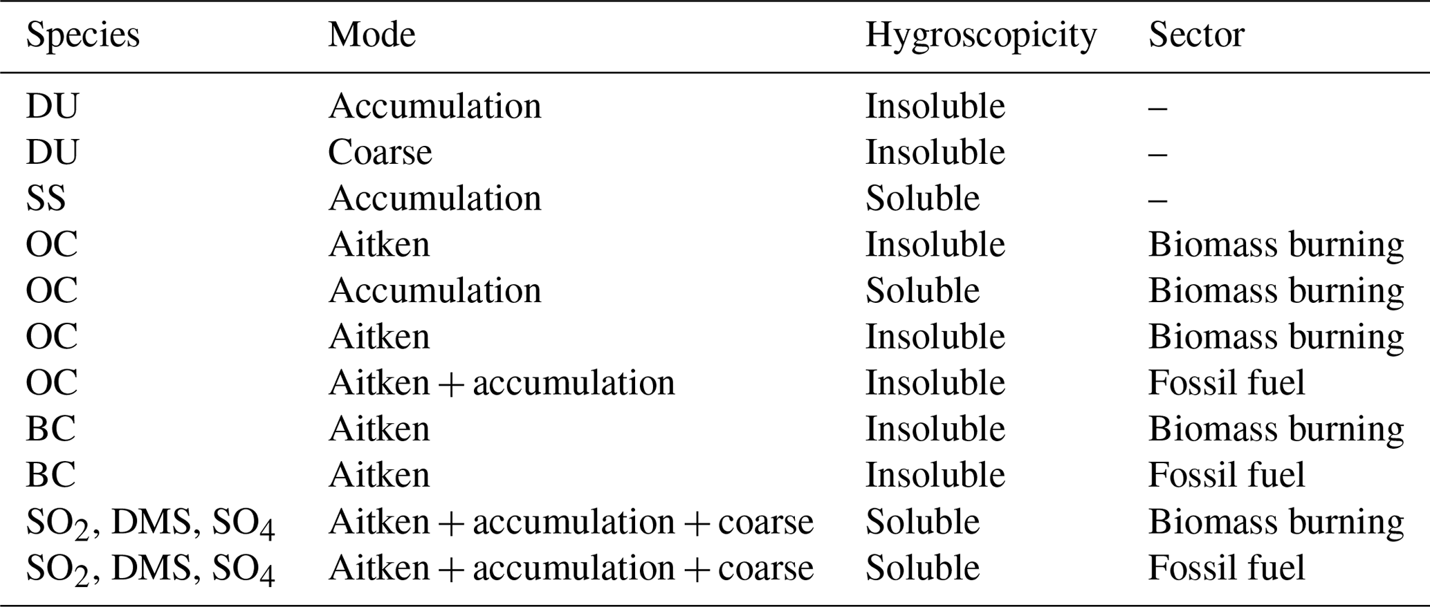
Table 1 Emission types that are distinctively perturbed and estimated (state vector) by the assimilation system. Fossil fuel refers to all emissions except biomass burning, which to a large extent includes mainly fossil fuel emissions but also other natural emissions like biogenic emissions. Biomass burning emissions include both natural and anthropogenic-induced fires. SO₂, DMS and SO₄ share the same perturbations but are distinctively defined for biomass burning and fossil fuel. The sulfates in the atmosphere are mainly produced by emitted SO₂, followed by DMS. Direct emissions of SO₄ are modeled as 2.5 % of the SO₂ emissions.

Table 2 Experiments overview.

New emission estimates are obtained by estimating scaling factors based on the assimilated observations by solving the following Kalman filter equations:

$$\begin{array}{}\text{(1)}& {\displaystyle }{\mathit{x}}_{\mathrm{a}}={\mathit{x}}_{\mathrm{b}}+{\mathbf{P}}_{\mathbf{a}}\cdot H^{\mathrm{T}}\cdot {\mathbf{R}}^{-\mathrm{1}}\cdot (\mathit{y}-H\cdot {\mathit{x}}_{\mathrm{b}}),\text{(2)}& {\displaystyle }{\mathbf{P}}_{\mathrm{a}}=(\mathbf{I}+{\mathbf{P}}_{\mathrm{b}}\cdot H^{\mathrm{T}}\cdot {\mathbf{R}}^{-\mathrm{1}}\cdot H{)}^{-\mathrm{1}}\cdot {\mathbf{P}}_{\mathrm{b}},\end{array}$$

where x_b is the background state vector and includes emission perturbations for each species (DU, SS, OC, BC and SO₄). Different perturbations are used for each optically relevant mode (Aitken, accumulation, coarse) and for biomass burning (BB) or fossil fuel (FF) contributions. Specifically, the emissions that are distinctively perturbed and estimated (11 in total) by the assimilation system are shown in Table 1. The perturbation of sulfate precursor gasses (SO₂ and DMS) used the same perturbations as SO₄. x_a is the analysis state vector, containing the retrieved emission scaling factors based on the assimilated observations (y). P_b and P_a are the covariance matrices corresponding to the background and analysis state vector, respectively. The observational uncertainties are represented by the error covariance matrix R. We assume R to be diagonal (i.e., correlations between observational errors are always assumed to be zero). The observation operator H translates the emission perturbations (x) into the simulated observations (H⋅x), and it is entirely handled by the model (emission, transport, deposition, aerosol processes and optical property code). T stands for the matrix transpose operator.

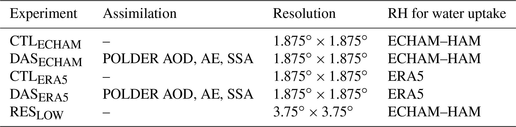
3.2 Experimental setup

All experiments are conducted using the model ECHAM–HAM for the year 2006. The experiments use 31 vertical sigma-hybrid levels from the surface to up to 10 hPa (troposphere-only simulations) and a T63 horizontal resolution of 1.875^∘ × 1.875^∘ and are nudged to ERA5 surface pressure as well as to vorticity, divergence and temperature for all vertical levels. A list of selected meteorological and aerosol options used for the experiments is presented in Table S1 in the Supplement.

CTL_ECHAM is an ECHAM–HAM run without data assimilation and with default settings, while DAS_ECHAM is a data assimilation experiment where the emissions are optimized based on measurements by POLDER. In addition, we conducted an experiment with an identical setup to CTL_ECHAM but with lower horizontal resolution (T31; 3.75^∘ × 3.75^∘).

CTL_ERA5 quantifies the effect of the underestimated relative humidity on aerosol optical properties in ECHAM compared with ERA5. CTL_ERA5 uses the relative humidity of ERA5 for aerosol water uptake. Note that this modification affects only the simulated aerosol optical properties in ECHAM–HAM, while the simulated water cycle (precipitation and evaporation) of the model remains unaltered. A data assimilation experiment based on this new CTL_ERA5 setup, named DAS_ERA5, was conducted in order to quantify the effect of the overestimated relative humidity profile on the aerosol emission estimation.

4 Results

4.1 Evaluating model fields with POLDER, AERONET and MODIS observations

All experiments were evaluated against the assimilated observations (POLDER) and independent observations (AERONET and MODIS). In both cases there is a significant improvement in all the aerosol optical properties in the DAS_ECHAM experiment, except for AE_550–865 over some land areas where the error increases. This can possibly be attributed to the relatively high observational uncertainty for AE_550–865 (Fig. A1).

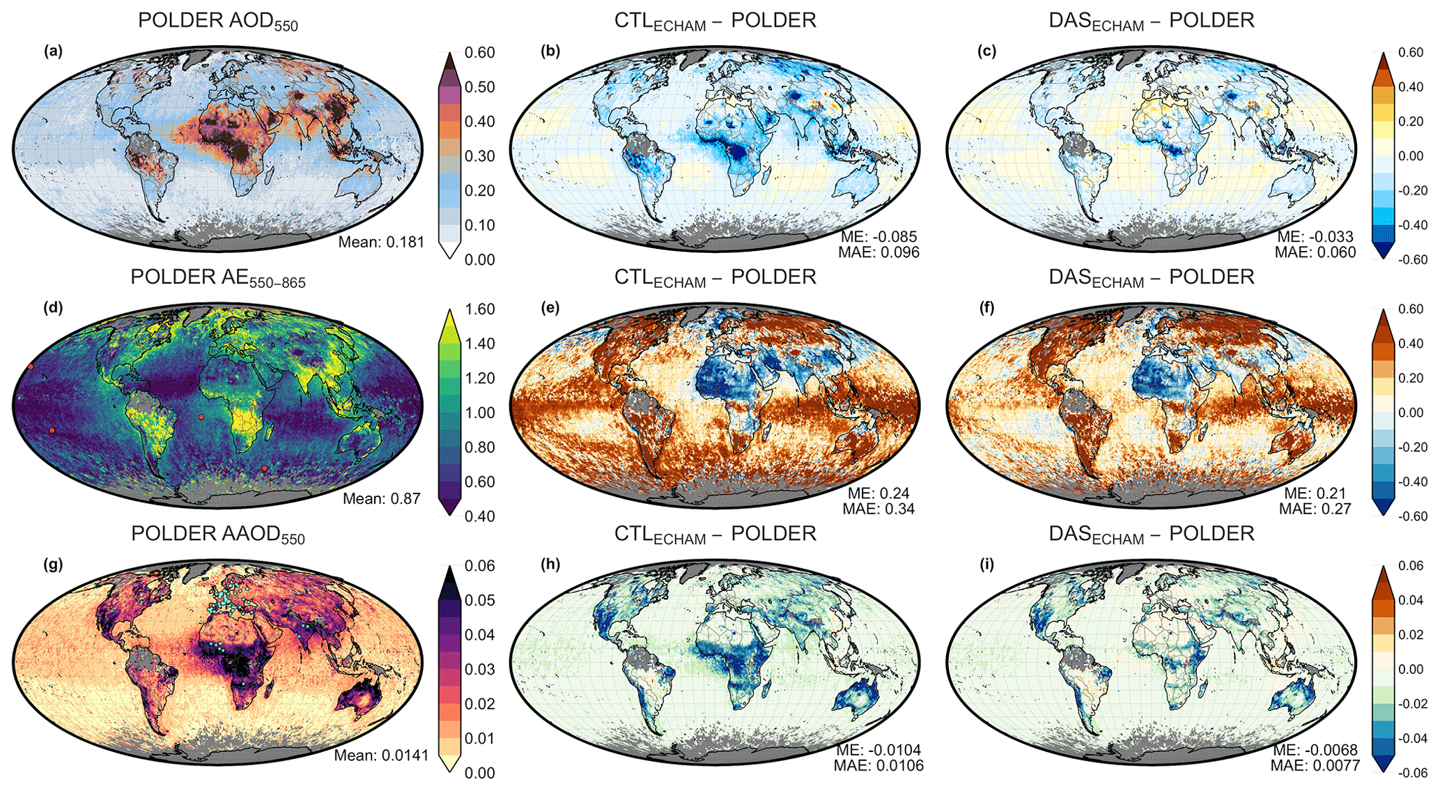
Figure 1 An evaluation of CTL_ECHAM and DAS_ECHAM experiments, based on POLDER for the year 2006. The first column depicts POLDER (a) AOD₅₅₀, (b) AE_550–865 and (c) AAOD₅₅₀, while the second and third columns display the differences between CTL_ECHAM − POLDER and DAS_ECHAM − POLDER, respectively. The global mean, global mean error (ME) and global mean absolute error (MAE) are depicted in the bottom-right corner of each plot. The points in panels (d) and (g) depict AERONET stations used for the plots of Figs. 3 and 4, respectively.

In Fig. 1 the experiments CTL_ECHAM and DAS_ECHAM are compared to the assimilated POLDER observations for the year 2006. CTL_ECHAM exhibits a strong underestimation in AOD over the biomass burning regions over the tropics (the Amazon, central Africa and Indonesia) and Siberia that are dominated by organic and black carbon aerosols, as well as over arid environments dominated by dust (the Sahara, the Middle East and the Taklimakan and Gobi deserts). AOD₅₅₀ is overestimated over southeastern China, where the aerosol load is very high (POLDER AOD₅₅₀ is higher than 0.6) and composed mostly of sulfates, as well as over open water bodies, where the aerosol load is low and dominated by sea salt. The CTL_ECHAM AOD₅₅₀ per species along with the optical depth due to condensed water on the surface of aerosol particles (WAT) are depicted in Fig. S1 in the Supplement. The assimilation of POLDER observations (DAS_ECHAM) reduces the AOD₅₅₀ global mean error (ME) from −0.08 to −0.03 and the mean absolute error (MAE) from 0.10 to 0.06, which shows that ECHAM–HAM can match the observations with adjusted emissions better. Note that the local improvement of AOD₅₅₀ for certain regions is even greater.

The AE_550–865 is a good proxy for aerosol size. High and low values of AE_550–865 relate to an aerosol load with more fine and more coarse particles, respectively. POLDER AE_550–865 is high over biomass burning and highly polluted regions, dominated mainly by OC, BC and SO₄, while it is low over the ocean and deserts where the aerosol load is primarily composed of DU and SS (Fig. 1d). In CTL_ECHAM, AE_550–865 is underestimated over the Sahara, the Middle East and eastern China, while it is overestimated over the ocean, Siberia, and North and South America. The estimated emissions by DAS_ECHAM improve the AE_550–865 difference over the ocean, and there is a significant improvement over China. The remaining high differences in AE_550–865 over land can be attributed to the high uncertainty in POLDER AE_550–865 over land. In Fig. S2 the yearly mean uncertainty in POLDER is depicted along with the MAE of the 3-hourly differences in CTL_ECHAM − POLDER and DAS_ECHAM − POLDER. The remaining MAEs of the 3-hourly differences in DAS_ECHAM (Fig. S2c) are on the same level as the POLDER uncertainty (Fig. S2a), which means that POLDER AE_550–865 over land is too uncertain to adjust emissions further. Additionally, sensitivity studies have shown that even when the biomass-burning-emitted particle size is altered aggressively in ECHAM–HAM, AE is not affected much (Zhong et al., 2022), which indicates that the emission changes may be less sensitive to the assimilation of AE_550–865 compared to AOD₅₅₀. The global MAE for AE_550–865 is reduced from 0.34 in CTL_ECHAM to 0.27 in DAS_ECHAM.

AAOD₅₅₀ is highly correlated with the BC aerosol load, which is the species that contributes up to 80 % of the total absorption globally, followed by DU (16 %) and OC (4 %) (Fig. S3). POLDER AAOD₅₅₀ peaks over tropical Africa and Sahel, where large biomass burning fires are active during the fire (dry) season. Fairly high values of absorption are also observed over the Amazon Basin for the same reason. Further, high AAOD₅₅₀ values are depicted over the northern and western coastline of Australia, which is probably a product of retrieval errors. Medium values of AAOD₅₅₀ that are related to anthropogenic emissions are visible over the eastern United States, Europe and eastern China. POLDER also depicts high AAOD₅₅₀ values over high-altitude regions (Schutgens et al., 2021), like the Rocky Mountains, the Andes, the Himalayas, the Zagros Mountains in Iran, the Hijaz Mountains in Saudi Arabia and the highlands in Ethiopia. Over these high-elevation areas there are hardly any BC or DU sources; thus these values might be a product of retrieval errors related to surface elevation.

AAOD₅₅₀ in CTL_ECHAM is mostly underestimated globally. A pronounced underestimation is evident over tropical Africa, which relates to the low BC emissions of the emission inventory that we use, GFAS (v1.0). Typically, the biomass burning emissions of GFAS for black and organic carbon are multiplied by a scaling factor of 3.4 to obtain a similar AOD to that observed by MODIS (Kaiser et al., 2012; Veira et al., 2015). Here this scaling factor is not applied in order to let our data assimilation system estimate new scaling factors based on POLDER observations, distinctively for OC and BC emissions. DAS_ECHAM has considerably smaller differences than POLDER globally and especially over the tropics. The global MAE for AAOD₅₅₀ is reduced from 0.0106 in CTL_ECHAM to 0.0077 in DAS_ECHAM.

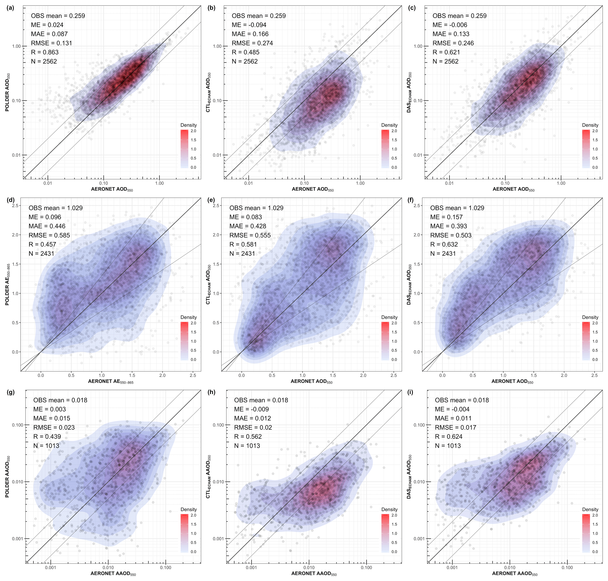
Figure 2 An evaluation of POLDER (first column), CTL_ECHAM (second column) and DAS_ECHAM (third column) based on AERONET for the year 2006. The first, second and third rows correspond to the variables AOD₅₅₀, AE_550–865 and AAOD₅₅₀, respectively. The OBS mean refers to AERONET in all plots. The mean error (ME), mean absolute error (MAE), root mean square error (RMSE), Pearson correlation (R) and the number of data points used in each case (N) are depicted in the top left of each subplot. The AOD₅₅₀ and AE_550–865 evaluation is based on the AERONET version 3 level 2.0 direct sun algorithm, while the AAOD₅₅₀ evaluation is based on the AERONET version 3 level 1.5 direct sun and inversion algorithm.

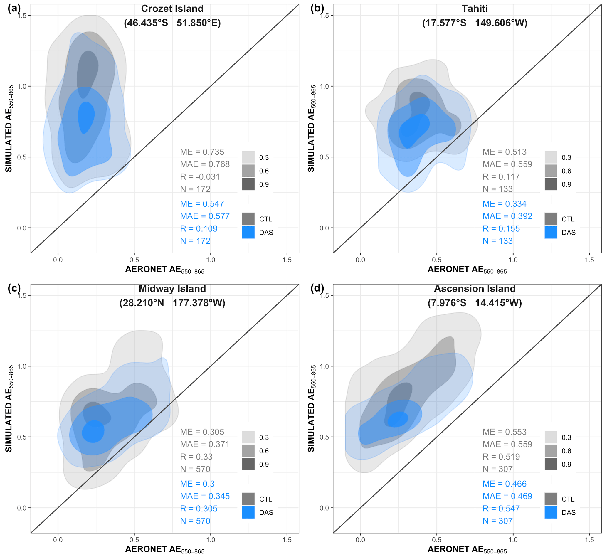
Figure 3 An AE_550–865 evaluation of CTL_ECHAM and DAS_ECHAM based on selected AERONET stations (red points in Fig. 1d) for the year 2006. These stations are located in isolated islands over the ocean in order to capture the changes in AE_550–865 due to SS emission changes. The shaded areas depict the 2D density estimate scaled to a maximum of 1 for 0.3, 0.6 and 0.9 intervals. The mean error (ME), mean absolute error (MAE), Pearson correlation (R) and the number of data points used in each case (N) are depicted for each subplot. The evaluation is based on the AERONET version 3 level 2.0 direct sun algorithm.

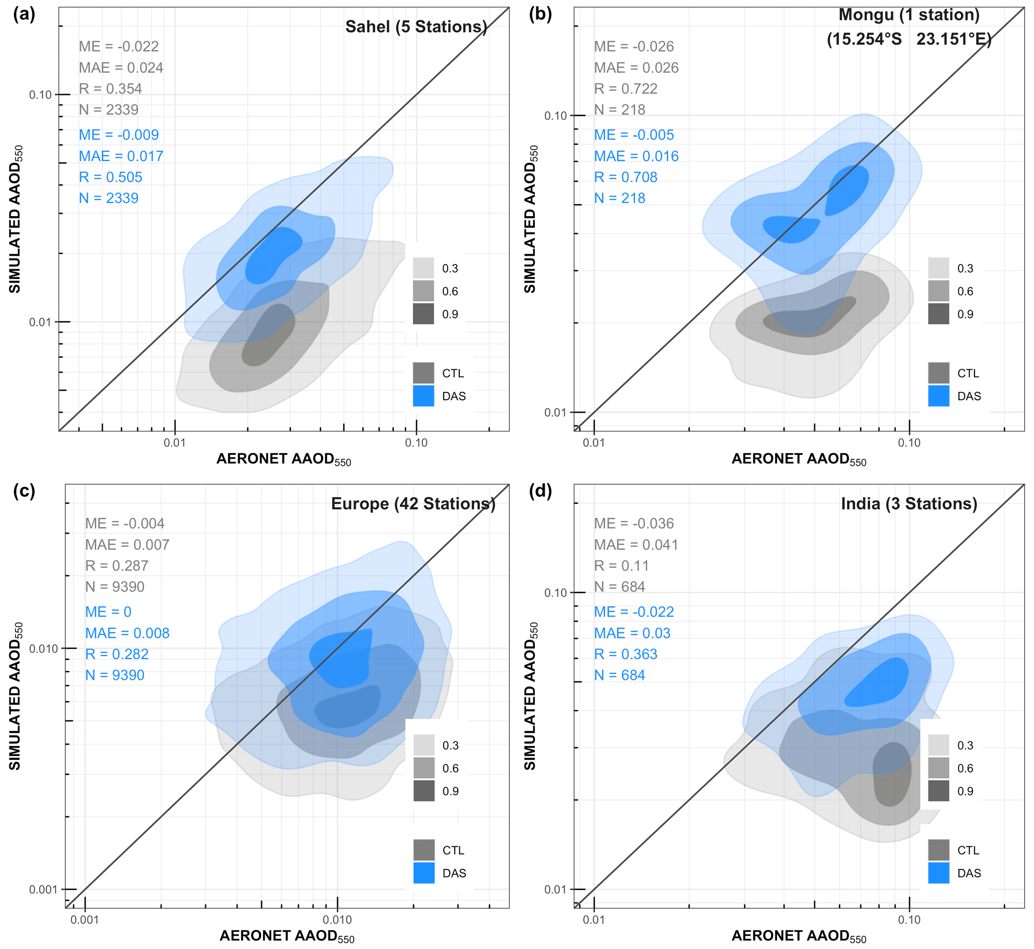
Figure 4 An AAOD₅₅₀ evaluation of CTL_ECHAM and DAS_ECHAM based on selected AERONET sites (cyan points in Fig. 1g) for the year 2006. These stations are selected over regions where natural and anthropogenic emissions of BC occur. The shaded areas depict the 2D density estimate scaled to a maximum of 1 for 0.3, 0.6 and 0.9 intervals. The mean error (ME), mean absolute error (MAE), Pearson correlation (R) and the number of data points used in each case (N) are depicted for each subplot. The evaluation is based on the AERONET version 3 level 1.5 direct sun and inversion algorithm.

The experiments are also evaluated with independent observations that are not assimilated. The scatterplots in Fig. 2 depict the evaluation of POLDER as well as the POLDER-collocated CTL_ECHAM and DAS_ECHAM against AERONET. All AERONET sites were collocated with the closest grid cell in one 1 × 1 resolution on a 3-hourly basis. Cases where multiple stations belonged to the same grid cell and had observations at the same time were averaged. A similar evaluation analysis against AERONET for model data that are not collocated to POLDER is provided in Fig. S4 for CTL_ECHAM and DAS_ECHAM. In addition Figs. 3 and 4 depict an evaluation of these two experiments for selected AERONET stations representative of SS and BC, respectively.

The ME and MAE improve in DAS_ECHAM experiments compared with CTL_ECHAM for all variables, except the AE_550–865 ME. The satellite AE_550–865 is overestimated compared with AERONET by 0.096, which can partially contribute to the increase in the AE_550–865 ME in DAS_ECHAM. Further, the unchanged high AE_550–865 in the model is observed over land (Fig. 2f) where the observational uncertainty in POLDER AE_550–865 is high (greater than 0.45) for most AOD₅₅₀ bins (Fig. A1).

The uncertainty in POLDER observations is based on an evaluation with AERONET (see Appendix A). POLDER AE_550–865 errors spread against AERONET (Fig. 2d) are similar to the CTL_ECHAM errors spread against AERONET (Fig. 2e). Notably the POLDER AAOD₅₅₀ errors spread against AERONET (Fig. 2g) are even greater than the CTL_ECHAM errors spread against AERONET (Fig. 2h). Despite this, there is a small improvement in MAE for both observables and a clear improvement in AAOD₅₅₀ bias where the ME goes from −0.009 in CTL_ECHAM to −0.004 in DAS_ECHAM.

The improvement in AE_550–865 and AAOD₅₅₀ compared with AERONET after data assimilation is much clearer if we focus on AERONET stations in regions where the difference between CTL_ECHAM and DAS_ECHAM is large. This is mostly in regions with strongly modified SS and BC emissions, respectively. To investigate this improvement, an evaluation for selected stations is depicted in Figs. 3 and 4. In Fig. 3 four stations that are located in isolated islands over the ocean were selected in order to capture the changes in AE_550–865 due to the adjusted SS emissions. In all cases CTL_ECHAM overestimates AE_550–865. After the adjusted emissions AE_550–865 is improved with a reduction in ME of about 0.1 or higher (except in Midway Island). In Fig. 4, four regions with biomass burning and anthropogenic BC emissions were selected to study the changes in AAOD₅₅₀. In all cases the underestimation of AAOD₅₅₀ in CTL_ECHAM improves after the adjusted emissions, especially in the sites over the biomass burning regions (Sahel stations and Mongu station), but also in regions with anthropogenic sources of BC (Europe and India). A similar improvement is observed for SSA₅₅₀ over the same regions (Fig. S5).

From previous work (Tsikerdekis et al., 2021), we know that assimilating AOD₅₅₀ along with AE_550–865 and SSA₅₅₀ results in a considerable AOD₅₅₀ improvement, with a small improvement in size and absorption. Assimilating only AOD₅₅₀ results in a considerable AOD₅₅₀ improvement, with a small improvement in aerosol size, while having a very negative effect on the aerosol absorption. Our findings here confirm the importance of assimilating information on size and absorption in addition to AOD. It is important to note that future polarimeter instruments such as SPEXone and 3MI are expected to yield better retrievals (Hasekamp et al., 2019) and hence have the potential to estimate aerosol emissions better (Tsikerdekis et al., 2022a).

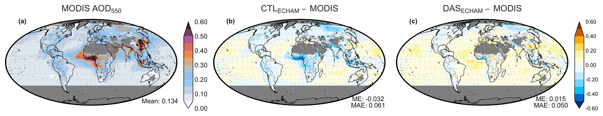
Figure 5 An evaluation of the CTL_ECHAM and DAS_ECHAM experiments, based on MODIS for the year 2006. The first column depicts MODIS AOD₅₅₀, while the second and third columns display the differences between CTL_ECHAM − POLDER and DAS_ECHAM − POLDER, respectively. The global mean, global mean error (ME) and global mean absolute error (MAE) are depicted in the bottom-right corner of each plot.

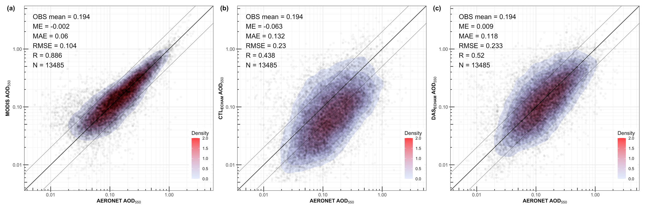
Figure 6 An AOD₅₅₀ evaluation of MODIS (first column), CTL_ECHAM (second column) and DAS_ECHAM (third column) based on AERONET for the year 2006. The OBS mean refers to AERONET in all subplots. The mean error (ME), mean absolute error (MAE), root mean square error (RMSE), Pearson correlation (R) and the number of data points used in each case (N) is depicted in the top left of each subplot. The AOD₅₅₀ evaluation is based on AERONET Version 3 Direct Sun Algorithm Level 2.0.

In addition, we evaluate the effect of the assimilation against MODIS Collection 5 Dark Target (Sayer et al., 2014) at 1^∘ × 1^∘ resolution. Specifically, we use a specialized version of MODIS designed for assimilation, which was corrected based on 4 years of AERONET observations (Hyer et al., 2011; Shi et al., 2011; Zhang and Reid, 2006). Figure 5 depicts the MODIS AOD₅₅₀ for the year 2006 along with the differences in CTL_ECHAM and DAS_ECHAM from MODIS. Before the assimilation the model biases against MODIS follow a similar pattern to the biases observed against POLDER, with an underestimation of AOD₅₅₀ over land (notably over biomass burning regions and Sahel) and an overestimation over the ocean. After the assimilation the negative bias over land is corrected, but the overestimation over the ocean remains. The ME and MAE improve from −0.032 and 0.061 in the CTL_ECHAM experiment to 0.015 and 0.050 in the DAS_ECHAM experiment. Further, we conduct a similar analysis to Fig. 2 but with the MODIS data. The scatterplots in Fig. 6 depict the collocated points between MODIS and AERONET for 2006, which are more than 5 times greater in number compared with POLDER. Similarly, before the assimilation a negative bias is observed, which is corrected after the assimilation with a reduction in the spread of the errors as well. Specifically, the ME is reduced from −0.063 to 0.009 and the MAE from 0.132 to 0.118.

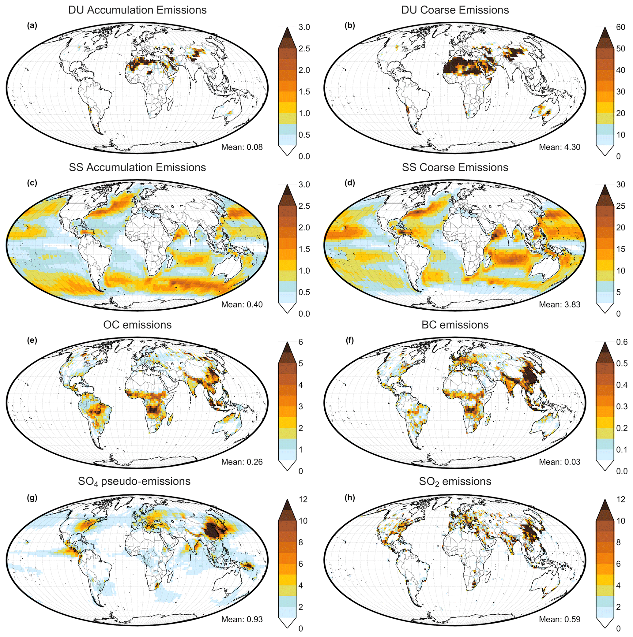
Figure 7 Aerosol emissions ($\mathrm{kg}{\mathrm{km}}^{-\mathrm{2}}{\mathrm{d}}^{-\mathrm{1}}$) of the CTL_ECHAM experiment for 2006. The global mean is depicted in the bottom-right corner of each map. The pseudo-emissions of SO₄ are based on the SO₄ total deposition.

4.2 Aerosol emission estimation from POLDER

The yearly emissions for several aerosol species are shown in Fig. 7. Dust and sea salt particles in the coarse mode dominate the total mass of aerosols, followed by sulfates and sea salt in the accumulation mode and organic carbon emissions. Note that sulfate total deposition is used as a proxy for sulfate formation in the atmosphere. SO₂ emissions are primarily concentrated over the Northern Hemisphere, mainly over North America, Europe, India and Southeast Asia. The black carbon total mass is very low globally (although it is very important for aerosol absorption; see Fig. S3) and is concentrated over biomass burning regions and densely populated areas where high anthropogenic emissions occur.

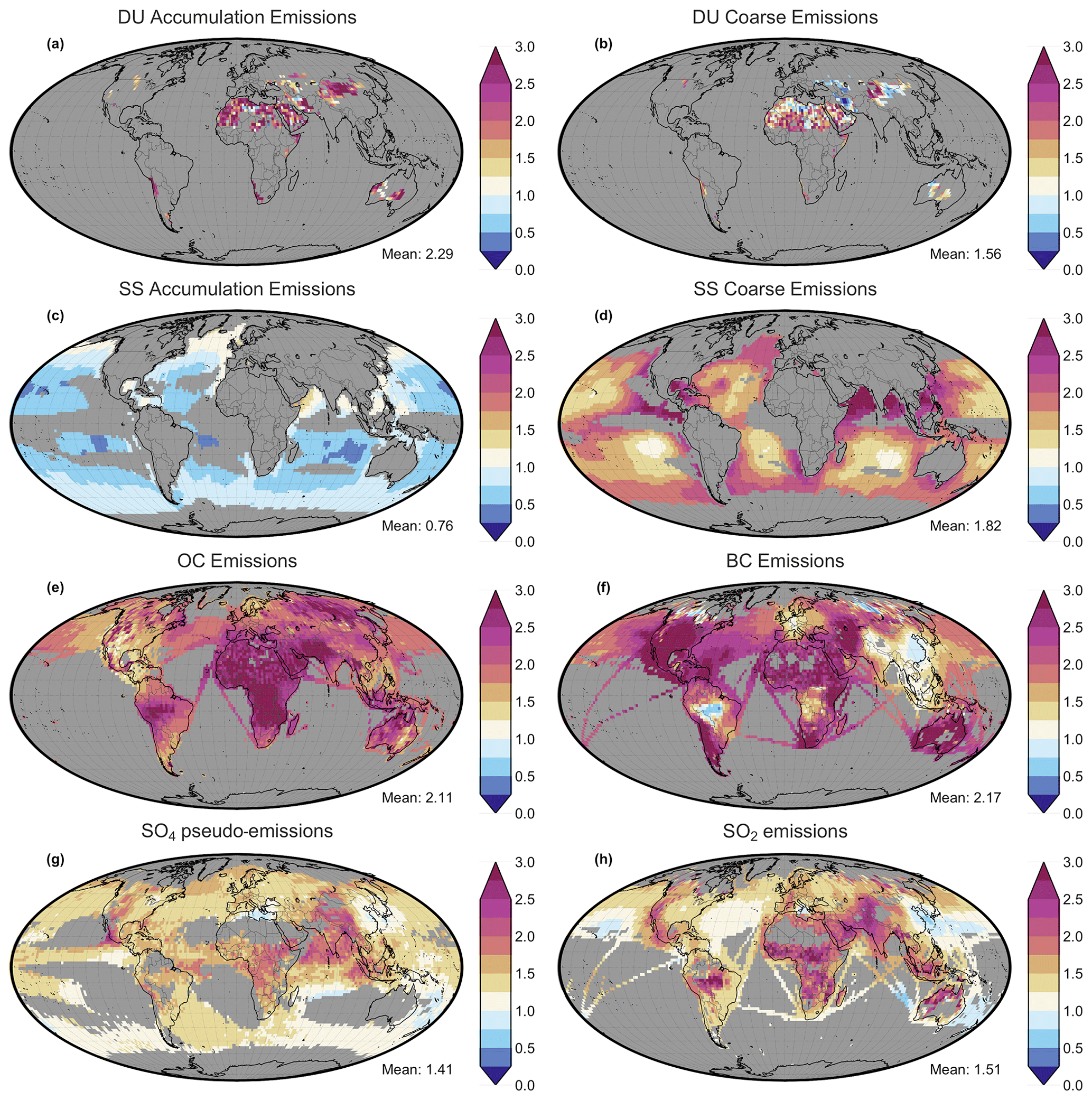
Figure 8 Relative changes in aerosol emissions due to the assimilated POLDER observations (DAS_ECHAM divided by CTL_ECHAM) for 2006. The global mean is depicted in the bottom-right corner of each map. Grey grid cells contain emissions lower than the global median value of each species and are excluded from these maps.

The relative changes in yearly aerosol emissions because of the assimilated POLDER observations are depicted in Fig. 8. Grid cells with emissions lower than the global median value in each species are masked out (grey) in order to emphasize areas where aerosol emissions are not too low. Overall, emissions increase for all species (except in the sea salt accumulation mode), which coincides with the large underestimation of both AOD₅₅₀ and AAOD₅₅₀ by CTL_ECHAM compared with POLDER (see Sect. 4.1).

Dust accumulation and coarse-mode emissions increase everywhere, except over Iran and the Gobi Desert during the coarse mode. Sea salt accumulation mode emissions are reduced almost everywhere in the world, while sea salt coarse-mode emissions increase. This illustrates the importance of assimilating the AE_550–865 observations, since these changes reduce the AE_550–865 overestimation compared with POLDER over the ocean. Organic carbon emissions increase everywhere globally and approximately by a factor of 3 in tropical Africa, 2.5 in the Amazon Basin and Indonesia, and 2 in Southeast Asia. Black carbon emissions increase approximately by a factor of 3 in the United States and 1.5 in tropical Africa and are slightly reduced in Southeast Asia and in parts of the Amazon Basin. In all cases the underestimated AAOD₅₅₀ of CTL_ECHAM improves in DAS_ECHAM. Note that POLDER AAOD₅₅₀ is overestimated over several high-altitude areas (as discussed in Sect. 4.1); thus emissions near these areas may have been inflated, since the correlation length of black carbon emissions perturbations in our data assimilation system is fairly big (25^∘). The SO₂ emissions increase in Europe as well as in North America by about a factor of 1.5 and remain almost the same over Southeast Asia. The same changes are observed for the SO₄ total deposition.

Considering the relatively big changes in emissions, ranging from 1.5 to 3.0 for large portions of the globe, and the small improvements when evaluating the observables with all AERONET stations, it can be concluded that the network spatial coverage may not be sufficient to capture the global aerosol changes. This may be more relevant for AE_550–865 and AAOD₅₅₀ than for AOD₅₅₀, where it is clearly improved (Fig. 2). Note that AE_550–865 and AAOD₅₅₀ also improve against AERONET when we focus on specific areas (Figs. 3 and 4).

4.3 Global aerosol emissions and comparison with other studies

In this subsection the new global-scale estimated emissions are presented and compared with previous studies. Some of these studies contain an ensemble of simulations (e.g., CMIP5, AEROCOM phase I and III), while others may include emissions based on data assimilation experiments. Note that the annual mean emissions for some studies may be regional and not global estimates (e.g., Chen et al., 2019; Escribano et al., 2017) and also may not refer to the year 2006, which is the reference year for our study. These issues, which are independent from inter-model differences in physics (e.g., emission schemes), chemistry parameterizations and prescribed emission inventories, may enhance the emissions differences from study to study. Thus, the comparison of our estimated emissions with the emissions from other studies is expected to differ and serves more as a qualitative comparison. The studies with an ensemble of models are presented in terms of the ensemble median, ensemble standard deviation and relative diversity, which is equal to the ratio of the standard deviation to the median and is then multiplied by 100.

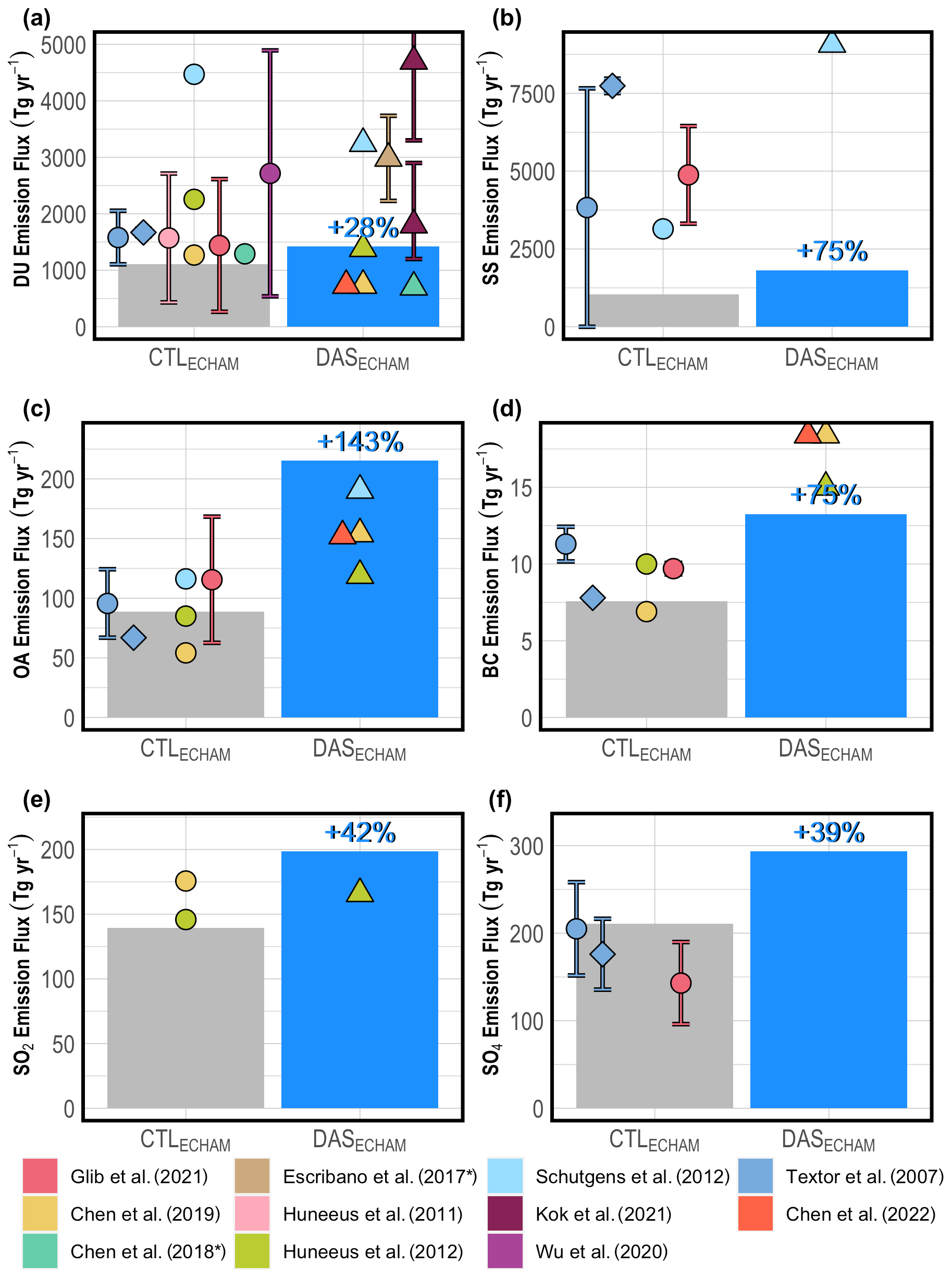
Figure 9 Global aerosol emissions in 2006 for dust (DU), sea salt (SS), organic aerosol (OA), black carbon (BC) and sulfur dioxide (SO₂) and the total deposition of sulfates (SO₄) (Tg yr⁻¹). The percentage change of the estimated emissions over DAS_ECHAM is estimated based on the emissions of CTL_ECHAM. The circles depict the reported emissions from other studies. The diamonds depict the sensitivity study in Textor et al. (2007), which is explained in the text. The triangles illustrate the emissions estimated from past data assimilation studies. OA is estimated by multiplying the emissions of OC by 1.4 for the experiments of this study, as well for the reported emissions in Schutgens et al. (2012) and Chen et al. (2019, 2022). The SO₄ total deposition is used as a proxy for SO₄ pseudo-emissions. SO₂ emissions for Chen et al. (2019) and Huneeus et al. (2012) were reported in Tg S yr⁻¹; thus they were multiplied by 2 in order to be converted into Tg SO₂ yr⁻¹. The asterisk symbol in some studies indicate that the reported emissions are regional and not global. The yearly emissions from Schutgens et al. (2012) are an extrapolation of a single month's (January) experiment. The two Kok et al. (2021) estimates refer to emissions for DU particles of up to 10 µm (low estimate) and up to 20 µm (high estimate) in geometric diameters (see text for more details).

4.3.1 Dust emissions

Dust (DU) and sea salt (SS) global emissions are shown in Fig. 9. The emissions of these species are highly dependent on the simulated aerosol size range of each model; the wind distribution in each model; and the activation areas, where dust can be emitted. Hence the emissions differ a lot from model to model (Wu et al., 2020). Previous studies have also indicated that emissions fluxes for DU and SS are also highly resolution dependent (Guelle et al., 2001; Laurent et al., 2008). Specifically, ECHAM–HAM showed that DU emissions may differ by a factor of more than 2 globally, with local changes in emissions being even higher between a simulation at T63 (CTL_ECHAM) to T31 (RES_LOW) horizontal resolution, while smaller local differences were observed in SS emissions (Fig. S6). It is important to note here that the emissions estimation for a lower-resolution (T31) data assimilation experiment (not shown) was very close (∼ 1500 Tg yr⁻¹) to the estimated emissions by the higher resolution (T63).

The global dust emissions of CTL_ECHAM are 1105 Tg yr⁻¹ and are increased to 1419 Tg yr⁻¹, a percentage change equal to 28 %. These changes bring emissions closer to the estimates of many other studies, as indicated with the different colored points in Fig. 9. The ensemble median of AEROCOM I (including 14 models) is 1572 Tg yr⁻¹, which lies quite close to the estimates of this study.

As with the AEROCOM I models, AEROCOM III tends to underestimate AOD and overestimate AE over the Sahara and Middle East according to AERONET, which suggests that the coarse aerosol emissions are underestimated relative to the fine-mode emissions (Gliß et al., 2021). The same can be seen in the CTL_ECHAM and DAS_ECHAM simulations (Fig. S7), with a mean error in AE_550–865 of 0.055 and 0.146, respectively, against AERONET. Note that POLDER AE_550–865 over the Sahara is biased high based on AERONET; thus these observations were not assimilated (see Appendix A). The overestimated AE_550–865 suggests that the estimated dust emissions in DAS_ECHAM should probably be higher, since the emissions of dust in the coarse mode, which correspond to 98 % of the total emitted dust globally, need to be higher.

The DU emissions ensemble median of CMIP5 models (15 models) is 2716 Tg yr⁻¹, with a 2177 Tg yr⁻¹ standard deviation and 80 % diversity (Wu et al., 2020). Some of the factors that contribute to this diversity are the difference in the simulated size range (e.g., from 0.06 to 63 µm for some models and < 16 µm for others), the global percentage where dust can be emitted that ranges from 2.9 % to 18 % and the differences in the spatial distribution of dust emissions.

The amount of the estimated dust emission due to data assimilation or observationally constrained methods in previous studies (Chen et al., 2018, 2019, 2022; Escribano et al., 2017; Huneeus et al., 2012; Schutgens et al., 2012) differs considerably both before and after observationally constraining the dust emissions for reasons that have already been discussed. In all these studies dust emissions change between 27 % and 62 % with a median value of 46 %. The percentage change of dust emissions due to the assimilated POLDER observations in the present study is 28 %, which lies in the lower end of the percentage change range of previous studies.

A recent study where dust emissions were constrained in terms of mass extinction efficiency, dust size distribution and dust optical depth has revealed the importance of including the very coarse particles (up to 20 µm in geometric diameter) for the total emitted dust mass in GCMs (Kok et al., 2021). According to the constrained experiment, 1800 Tg yr⁻¹ (with a 1σ uncertainty between 1200 and 2700 Tg yr⁻¹) was reported for emissions of up to 10 µm, which is close to our estimate and the ensembles of other studies. In contrast, for emissions of up to 20 µm, 4700 Tg yr⁻¹ (with a 1σ uncertainty between 3300 and 9000 Tg yr⁻¹) was reported. The contribution of emitted particles between 10 and 20 µm to the total dust emissions was close to 65 %, but the contribution to the total AOD₅₅₀ in the same size range was about 7 %. Based on these results, the inclusion of a super-coarse insoluble mode in ECHAM–HAM will increase total emissions and AOD₅₅₀ over dust areas as well as the estimated emissions by our data assimilation system. The inclusion of coarse dust particles (> 10 µm) in GCMs is crucial for the total mass of dust emissions, absorption (Kok et al., 2021) and the nutrient contribution of dust to land and ocean ecosystems (Kim et al., 2014), but in terms of dust scattering the effect would be quite limited since their mass extinction efficiency relative to smaller particles is considerably smaller (particularly for the shortwave radiation).

4.3.2 Sea salt emissions

The SS emissions for the CTL_ECHAM experiment is 1039 Tg yr⁻¹, which in comparison with the other studies is considerably lower. The coarse mode, which contains 90 % of the total emission mass of SS, is probably underestimated in the sea salt scheme that was used for our experiments (Long et al., 2011). This is also supported from an evaluation with POLDER, where the CTL_ECHAM experiment overestimated AE_550–865 over the ocean (Fig. 1e). The ensemble median of AEROCOM III is 4880 Tg yr⁻¹ (excluding ECMWF-IFS), with a standard deviation of 1568 Tg yr⁻¹ and a diversity of 32 % (Gliß et al., 2021). ECMWF-IFS with an estimate of 50 000 Tg yr⁻¹ was not included since the emission scheme (Grythe et al., 2014) produces SS particles that are too large and that have very short lifetimes (Gliß et al., 2021). Note that the AEROCOM III ensemble median tends to underestimate the AE by 22 %, mainly over the ocean, according to AATSR-SU observations, thus overestimating the SS particle size and to an extent the mass flux of emissions (Gliß et al., 2021). Based on a fraction of AEROCOM I models, Textor et al. (2007) estimated an ensemble median of 3830 Tg yr⁻¹ with a standard deviation of 3830 Tg yr⁻¹ that results in a diversity of 100 %.

The assimilation of POLDER observations increases the global emissions to 1850 Tg yr⁻¹ in DAS_ECHAM, which corresponds to a percentage change of +82 % with respect to the CTL_ECHAM experiment. Although SS emissions are still low (compared with the majority of AEROCOM III models, for example), ECHAM–HAM can reproduce the AOD adequately both before and after the assimilation (Fig. 1b and c), indicating that the mass extinction coefficient (MEC) of the model is high. A high MEC is related to more fine SS particles, as indicated by the evaluation against POLDER AE_550–865 (Fig. 1). Further, a high MEC could partially be explained by the overestimated RH that enhances water uptake into SS and increases AOD. This topic is discussed further in Sect. 4.4. So far only one data assimilation study has provided an aerosol emission estimate. Schutgens et al. (2012) found that the SS emissions increased after assimilating AERONET stations and MODIS-Aqua AOD over the ocean. It is noteworthy that their yearly emissions were estimated from a monthly (January 2009) experiment.

4.3.3 Organic aerosol emissions

In order to compare our emissions with other studies, OC emissions were converted to organic aerosol (OA) by multiplying them by a factor of 1.4 (Tegen et al., 2019). The OA global emission from the CTL_ECHAM run is equal to 88.6 Tg yr⁻¹. The AEROCOM III ensemble median is 116 Tg yr⁻¹, with a large standard deviation (53 Tg yr⁻¹) and diversity (46 %). Inter-model differences between the AEROCOM III models are associated with differences in initial primary organic aerosol emissions, differences in secondary organic aerosol formation and differences in the conversion of OC from diverse sources of OA (Gliß et al., 2021). For example, the conversion factors used to convert OC to OA can range between 1.4 and 2.6. These values are used by many AEROCOM III models that multiply all OC emissions, independently of the source type. But there are also models (e.g., NorESM2) that use different conversion factors depending on the source type, for example, 1.6 for fossil fuel sources and 2.6 for biomass burning sources (Gliß et al., 2021).

The assimilated POLDER observations increase the OA emissions to 215.2 Tg yr⁻¹ (+143 %) in DAS_ECHAM, which is higher than in any other emission estimation study. All previous data assimilation studies have indicated an increase in OA emissions when observations are considered. The amount of increase differs from study to study, but the increasing signal is apparent in all, independently of the observations that were assimilated in each case. The emissions in Schutgens et al. (2012), Chen et al. (2019) and Chen et al. (2022) are reported in OC; thus they were multiplied by 1.4 to get an approximation of the OA emissions. The OA emissions increase in Schutgens et al. (2012) from 116.2 to 190.4 Tg yr⁻¹ (+64 %), in Huneeus et al. (2012) from 85 to 119 Tg yr⁻¹ (+40 %) and in Chen et al. (2019) from 54.2 to 153.9 Tg yr⁻¹ (+184 %). Note that the increase in organic aerosol emissions in DAS_ECHAM is significantly stronger for natural biomass burning sources (+193 %) than for anthropogenic sources (+115 %).

4.3.4 Black carbon emissions

The black carbon (BC) global emission is 7.6 Tg yr⁻¹ for the CTL_ECHAM experiment. Since BC is highly absorbing, the estimated emissions will highly depend on the assimilation of SSA (or AAOD). Aerosol absorption information can be obtained by POLDER, and, as shown previously, the assimilation of absorbing observations is essential in order to correctly estimate the BC mixing ratio and accurately simulate the absorption in a model (Tsikerdekis et al., 2021). The CTL_ECHAM experiment underestimates AAOD₅₅₀ compared with POLDER; thus the BC emissions increase in DAS_ECHAM to 13.3 Tg yr⁻¹ (+75 %). Previous data assimilation studies have shown a similar increasing tendency to OC emissions. Specifically, the BC emissions increase in Huneeus et al. (2012) from 10 to 15 Tg yr⁻¹ (+50 %) and in Chen et al. (2019) from 6.9 to 18.4 Tg yr⁻¹ (+166 %).

Note that the biomass burning emissions of organic and black carbon are based on GFAS emissions. The biomass burning emissions in DAS_ECHAM increase by 193 % and 90 % (not shown) compared with CTL_ECHAM, which correspond to scaling factors equal to 2.93 and 1.90, respectively. These new scaling factors are distinctively estimated for organic and black carbon and are based on the assimilation of POLDER observations that includes absorption information; they can thus be used by future studies to scale the GFAS emissions. Past studies have proposed a scaling factor of 3.4 for GFAS emissions based on an AOD evaluation (Kaiser et al., 2012; Tegen et al., 2019; Veira et al., 2015), which was not applied in this study in order to estimate new scaling factors based on the assimilation of POLDER observations.

4.3.5 Sulfates and precursors emissions

The total deposition of SO₄, which we use as a proxy for SO₄ pseudo-emissions, or rather the total chemical production of SO₄ in the atmosphere, along with the global emissions of SO₂, are depicted in Fig. 9. The global pseudo-emission of SO₄ is 210.9 Tg yr⁻¹ for CTL_ECHAM. The pseudo-emission of SO₄ for the AEROCOM III ensemble median for the year 2010 is 143 Tg yr⁻¹, with a standard deviation of 46.9 Tg yr⁻¹ and a diversity of 33 % (Gliß et al., 2021). ECHAM–HAM and ECHAM–SALSA have among the highest SO₄ pseudo-emissions in this ensemble (218 and 216 Tg yr⁻¹, respectively), which indicates that the production of SO₄ from SO₂ is possibly higher or SO₂ loss is possibly lower in these two models compared with the other AEROCOM III models. Further, Textor et al. (2007) noted that the differences in SO₄ production among AEROCOM I models remain almost the same, even when the same prescribed emissions of SO₂ are used, thus highlighting that inter-model differences in SO₄ may primarily be caused by differences in gain and loss processes rather than by differences in the primary SO₂ emissions. The production and loss processes of SO₄ are discussed in more detail in Sect. 4.4.2.

The SO₂ emission of CTL_ECHAM is 139.6 Tg yr⁻¹. The respective value for the CEDS emission inventory used by the CMIP6 models is 123.4 Tg yr⁻¹ (not shown in Fig. 9). The SO₂ emissions in the HTAP v2 emission inventory for 2010 used in Chen et al.'s (2019) study are higher (175.6 Tg yr⁻¹) than CTL_ECHAM, while SO₂ emissions in Huneeus et al. (2012) for 2002 are closer (145.8 Tg yr⁻¹) compared with CTL_ECHAM. Only the later study has provided a new estimate for SO₂ emissions based on the assimilation of total and fine AOD of MODIS, which increased the SO₂ emissions to 165.8 Tg yr⁻¹ (+14 %). In DAS_ECHAM the SO₂ emissions increase to 198.4 Tg yr⁻¹ (+42 %), which is higher than the reported emissions of Chen et al. (2019) and Huneeus et al. (2012).

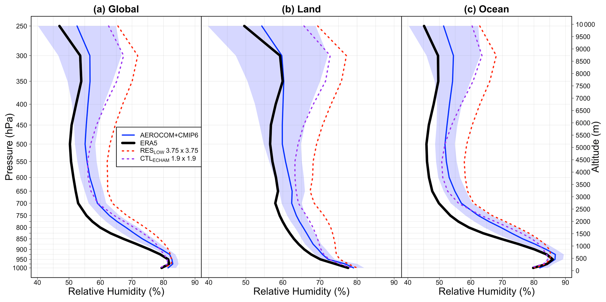
Figure 10 The relative humidity profile for a multi-model ensemble mean from 15 simulations that includes AEROCOM III and CMIP6 models (blue) along with ERA5 (black) for the year 2010. The shaded area represents the standard deviation of the ensemble. The CTL_ECHAM and RES_LOW experiments are also depicted.

4.3.6 Overestimated relative humidity and the impact on aerosol optical properties

In this subsection we investigate the effect of errors in relative humidity and resulting errors in aerosol water uptake on the estimated emissions. In Fig. 10, we compare the mean and standard deviation of the relative humidity profiles of ECHAM, AEROCOM (eight models) and CMIP6 (seven models) with ERA5. ERA5 is set as the reference, and since it is a reanalysis product where numerous meteorological observations were assimilated and compared with all the other GCMs, the simulated RH should be closer to the truth. The majority of the models in this ensemble overestimates RH, both over land and over the ocean (Fig. 10c and b), except the AEROCOM III simulation conducted with the GFDL-AM4, GEOS and MIROC-SPRINTARS models, where the simulated profile of relative humidity is closer to ERA5, and their horizontal resolution is at least 2 times higher compared with the other simulations. None of the models underestimates the RH profile compared with ERA5. In addition to this ensemble, ECHAM–HAM simulations conducted for the year 2006 with different horizontal resolutions are also shown (CTL_ECHAM, RES_LOW). Clearly there is a dependence between the horizontal resolution of ECHAM–HAM and its capability to accurately simulate RH profiles. It is known that the current horizontal resolution of GCMs cannot directly resolve humidity's small-scale spatial variability; thus it is parameterized (Lin, 2014). This is probably what is causing the differences in the RH profile compared with ERA5, but this is a topic that is out of the scope of our study. Note that the interannual ERA5 RH variability for the years 2006 (current study experiments) and 2010 (AEROCOM III) is minuscule (not shown).

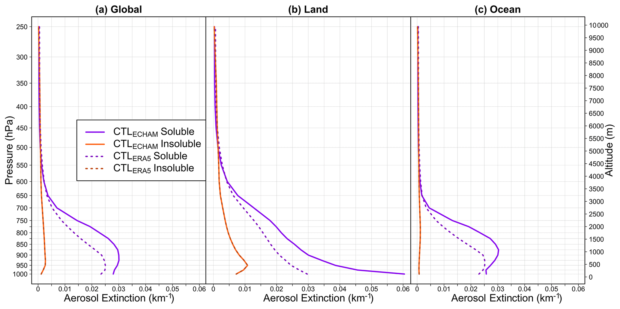
Figure 11 Aerosol extinction profiles (km⁻¹) of CTL_ECHAM and CTL_ERA5 for soluble and insoluble aerosols.

The overestimation of RH for aerosol water uptake is the most critical for the lower troposphere (< ∼ 3 km or about 700 hPa), where RH is high enough (> 50 %) for water uptake to be relevant (Fig. 11) and where most of the soluble aerosols exist. This overestimation is mostly concentrated over the ocean (Fig. S8), but there are also land areas where substantial overestimation of relative humidity is observed (e.g., East Asia). In order to quantify how aerosol properties are affected by the overestimation of the RH profile by ECHAM–HAM, an additional experiment (CTL_ERA5) that used the RH profile of ERA5 to determine the growth factor in ECHAM–HAM was conducted. Note that this modification affects only aerosol optical properties (scattering and absorption) in ECHAM–HAM, while the water cycle (precipitation and evaporation) of the model remains unaltered.

Figure 11 depicts the mean aerosol extinction profile for the CTL_ECHAM and CTL_ERA5 experiments. The aerosol extinction of insoluble particles is identical between the two experiments since they remain unaffected by aerosol water uptake changes. In contrast, the aerosol extinction of soluble particles in CTL_ERA5 exhibits considerably lower aerosol extinction compared with CTL_ECHAM. Over land this difference reaches the maximum close to the surface and declines with height to up to 600 hPa (∼ 3800 m) where it becomes zero. Over the ocean, the difference is small close to the surface, peaks at 825 hPa (∼ 1500 m) and slowly declines to up to 650 hPa (∼ 3200 m) where it becomes zero.

Note that over the ocean ECHAM–HAM strongly overestimates RH profiles consistently over most grid cells, enhancing the growth of aerosols, which are mainly SS aerosols. In contrast, over land RH is overestimated in East Asia, Europe and the eastern part of North America, where soluble SO₄ production is high, and underestimated over Sahel and the western part of the United States where insoluble DU particles are not affected by water uptake (Fig. S1). Consequently, over the ocean aerosol extinction profile differences (Fig. 11c) match the overestimation of RH by ECHAM–HAM (Fig. 10c), while over land this is not the case (Figs. 11b and 10b). Most interestingly, over high-density population areas (eastern China, Europe, North America), where high emissions of anthropogenic SO₂ (precursor of SO₄) occur, the aerosol extinction difference between CTL_ECHAM and CTL_ERA5 is even greater, indicating that aerosol extinction of anthropogenic-induced aerosols is incorrectly inflated in ECHAM–HAM (and possibly in many other GCMs) because of the RH overestimation.

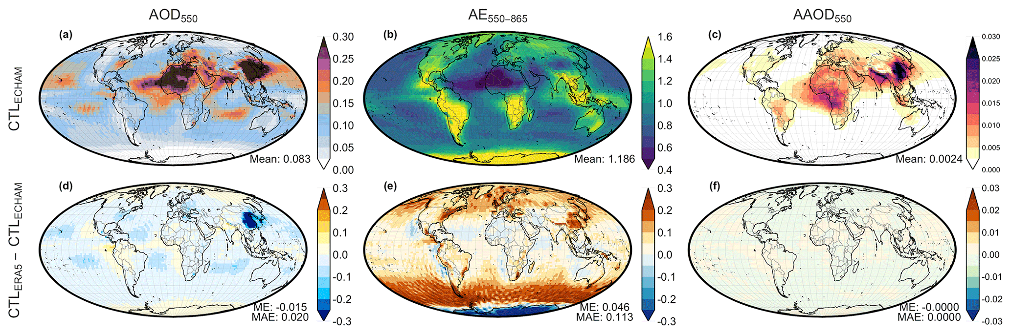
Figure 12 Aerosol optical properties of CTL_ECHAM and the differences between CTL_ERA5 and CTL_ECHAM.

The global contribution of water condensed on the surface of aerosol particles (WAT) to total AOD₅₅₀ changes from 62 % to 52 % from the CTL_ECHAM experiment to the CTL_ERA5 experiment. For reference, the contribution of water AOD₅₅₀ to total AOD₅₅₀ in K. Zhang et al. (2012) was reported to be 70 % using ECHAM5–HAM2, which was nudged to ERA-40 for the year 2000. Although a 10 % decrease is significant, water aerosol optical depth remains the largest contributor of total AOD₅₅₀ in CTL_ERA5, followed by DU (27 %), SO₄ (11 %), OC (5 %), SS (5 %) and BC (1 %).

Changes in AOD₅₅₀, AE_550–865 and AAOD₅₅₀ because of the overestimated RH are depicted in Fig. 12. Globally AOD₅₅₀ is reduced by 0.015 (18 %); AE_550–865 increases by 0.046; and AAOD₅₅₀ is virtually unchanged, since BC and DU, which contribute 96 % of the global AAOD₅₅₀ (Fig. S3), are insoluble. Regionally, the AOD₅₅₀ change is by far the strongest over East Asia, which can be explained by the presence of large loading of hydrophilic SO₄ aerosol particles (Fig. S1e). The same holds, to a lesser extent, for the eastern part of North America and Europe. Over the ocean, the largest AOD changes correspond to regions with a high concentration of SS aerosols (Fig. S1b), within the tropics and at high latitudes. AE_550–865 is affected by strong changes in the poles, where aerosol concentration is very low, so the global mean values are a bit misleading. AE_550–865 also increases over East Asia, Europe and the eastern part of North America.

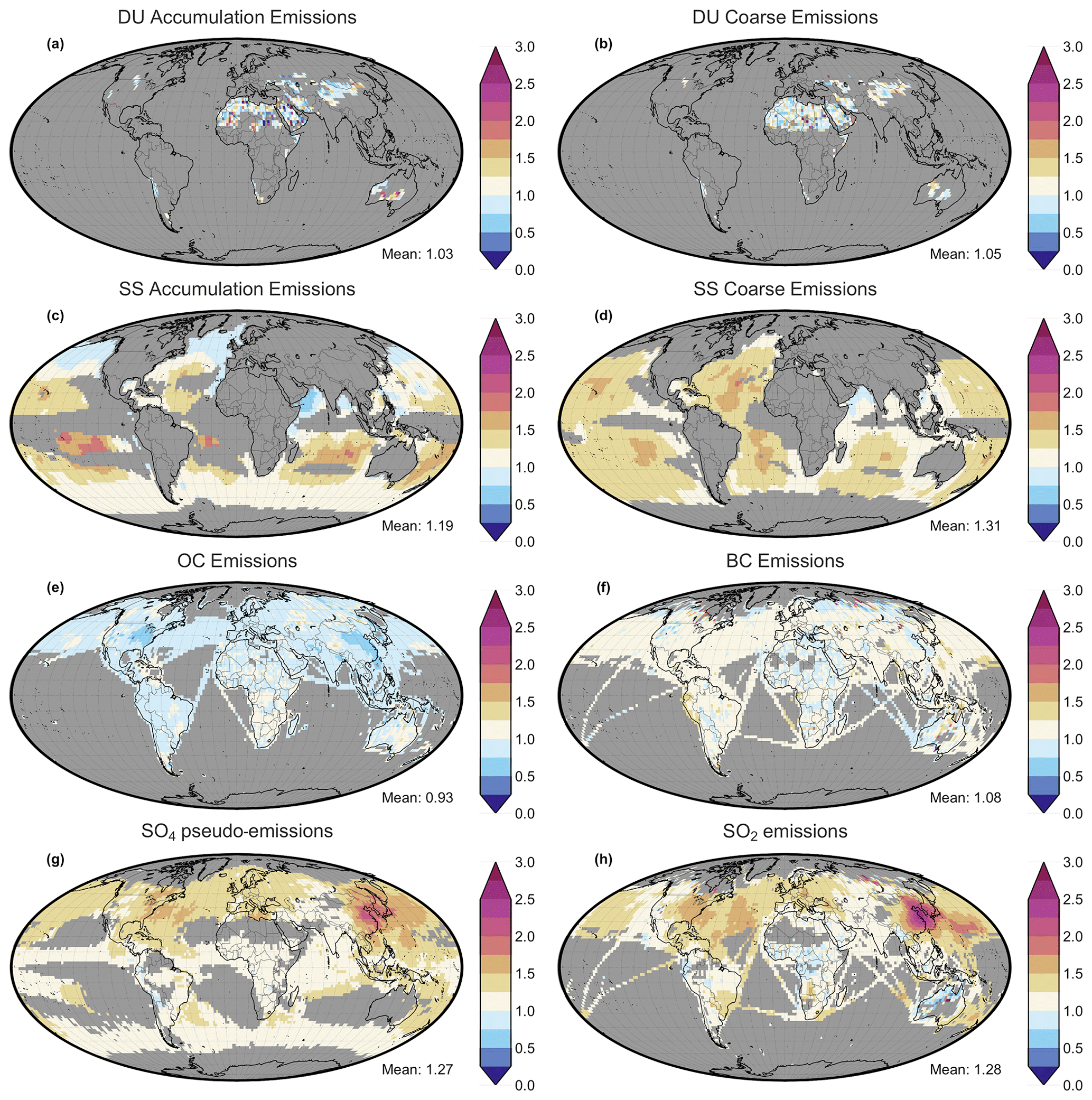
Figure 13 Relative changes in aerosol emissions after accounting for the correct relative humidity for aerosol water uptake (DAS_ERA5 divided by DAS_ECHAM) for 2006. The global mean is depicted in the bottom-right corner of each map. Grey grid cells contain emissions lower than the global median value of each species and are excluded from these maps.

4.3.7 Changes in emissions when considering the corrected relative humidity

An additional data assimilation experiment was conducted using the relative humidity from ERA5 (assumed to be the most accurate data available) in order to describe aerosol water uptake. The relative changes in aerosol emissions for this DA experiment (DAS_ERA5) compared with the standard DA experiment (DAS_ECHAM) are depicted in Fig. 13. These changes are quantified by the ratio of DAS_ERA5 to DAS_ECHAM. The evaluations of aerosol optical properties of DAS_ECHAM and DAS_ERA5 against POLDER and AERONET are very similar (not shown), suggesting that the emissions had to change differently in each experiment in order to compensate for the distinct differences in RH that affected aerosol optical properties.

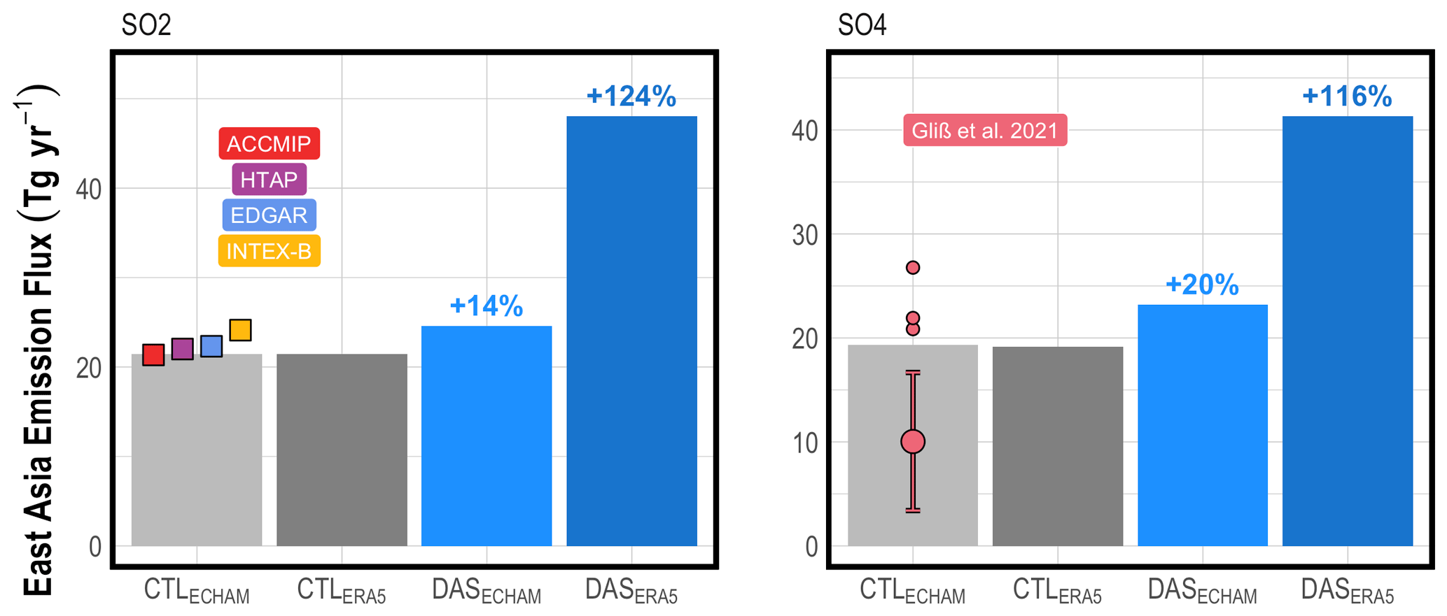
Figure 14 Aerosol emissions over China for SO₂ and SO₄ (Tg yr⁻¹). The percentage change of the estimated emissions over DAS_ECHAM and DAS_ERA5 is estimated based on the emissions of CTL_ECHAM and CTL_ERA5, respectively. The bars show the sum of the emissions for eastern China (24 to 44^∘ N, 100 to 120^∘ E). The squares depict the annual emissions of 2006 for four bottom-up inventories (ACCMIP, HTAP, EDGAR and INTEX-B) over the same domain as reported in Chang et al. (2015).

As expected, strong changes occur in the soluble particles, SS and SO₄. Overall, both the accumulation and the coarse-mode emissions of SS increase almost everywhere over the ocean. The increase in the accumulation mode is more pronounced in the Southern Hemisphere. The considerable difference between the two DAS experiments is caused by the fact that in DAS_ERA5 aerosol particles are smaller (less water) and hence less efficient in the extinction of light. So, more emissions of more particles are needed to match the measured AOD₅₅₀ by POLDER. The global SS emission in the DAS_ERA5 experiment is 2317 Tg yr⁻¹.

As for SO₄, DAS_ERA5 emissions distinctively increase over Southeast Asia by about 2 and to a lesser extent in Europe and North America (Fig. 13g and h). The results over Southeast Asia are particularly interesting, since they could hint at a potential big error in the bottom-up emissions inventories and/or could reveal underlying model errors with different signs that compensate for each other. These changes are discussed in Sect. 4.4.2 using additional evaluations with independent observations. The emission changes in the insoluble species (DU and BC) remain almost unchanged. Additionally, a very small reduction is observed for OC over North America and Southeast Asia, which barely reduces the AOD₅₅₀ by about 0.01.

4.3.8 Sulfate emissions in East Asia

In this subsection we use additional observational datasets to evaluate the model over East Asia, and we further investigate the estimated emissions of SO₄ by DAS_ERA5 over Asia. Note that most of the SO₂ sources are in the eastern part of China (Fig. 7h). The emissions of SO₂ and SO₄ for a part of East Asia are depicted in Fig. 14. Additional SO₂ estimates from bottom-up estimates are provided for comparison. DMS emissions are not shown, since they contribute a very small fraction (about 3 %) to the mass production of SO₄ and mostly over the ocean.

The two CTL experiments and DAS_ECHAM are within the range of previously reported estimates, while the SO₂ and SO₄ emissions in DAS_ERA5 more than doubled compared with CTL_ERA5 (Fig. 14). As already discussed, these large changes are caused by using more accurate relative humidity profiles for aerosol water uptake, which reduce AOD₅₅₀ significantly over the area, and, consequently, the emission estimation system compensates for it by increasing SO₂ and SO₄ emissions. But since the uncertainty in the bottom-up emission inventories is only 5.3 % for eastern China (Chang et al., 2015), it is highly unlikely that DAS_ERA5 emissions are correct.

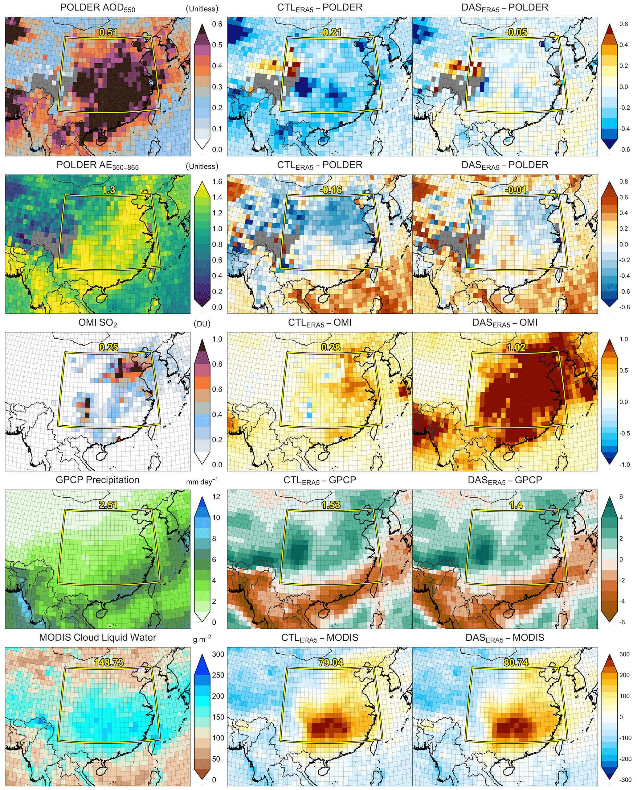
Figure 15 The (a) POLDER AOD₅₅₀, (b) POLDER AE_550–865, (c) OMI SO₂ in Dobson units, (d) GPCP precipitation and (e) MODIS-Terra cloud liquid water over eastern China. The second and third columns show the differences between CTL_ERA5 − observations and DAS_ERA5 − observations, respectively. The number within each figure refers to the mean value of the yellow polygon in each case.

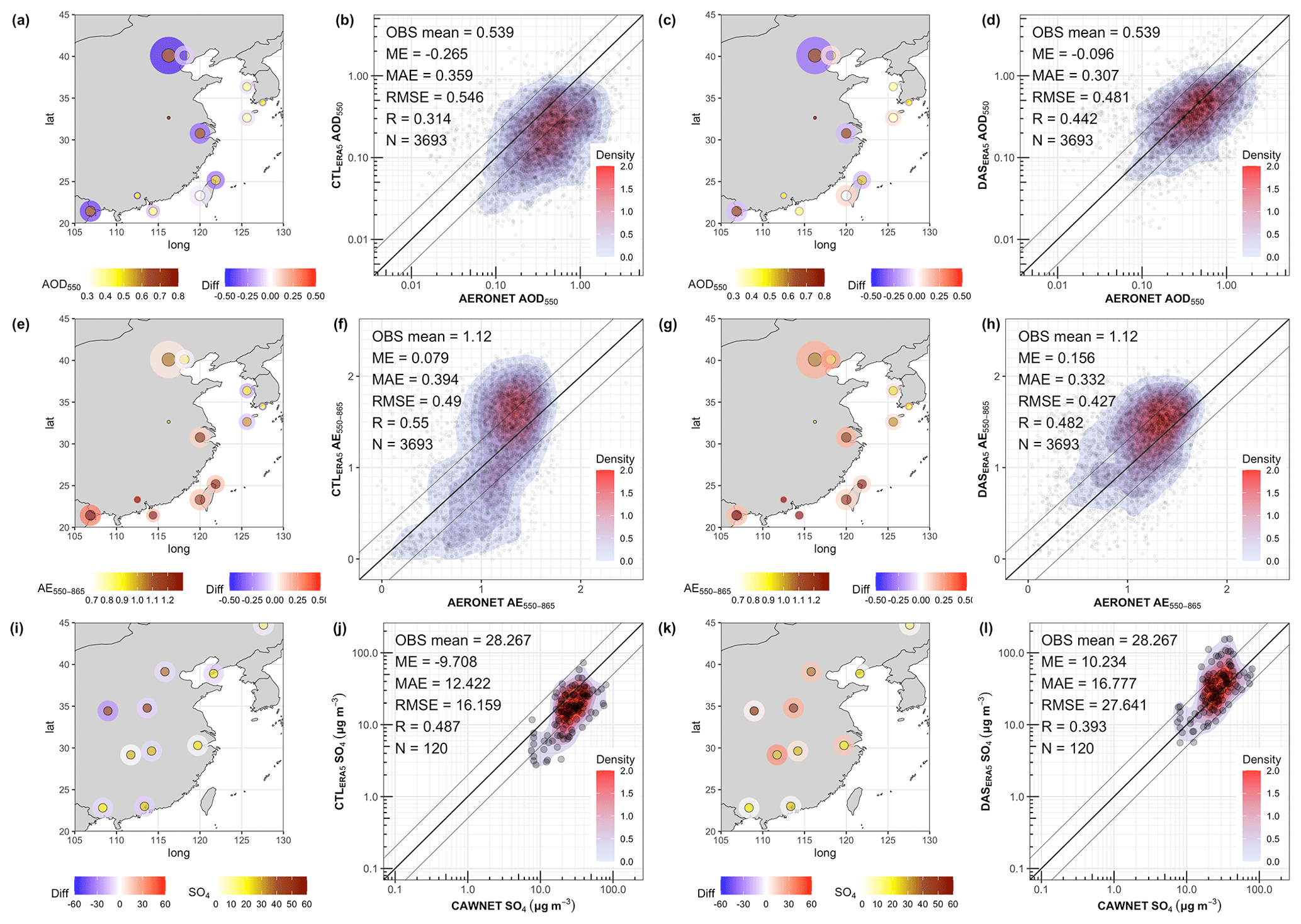
Figure 16 An evaluation of the CTL_ERA5 and DAS_ERA5 experiments for AOD₅₅₀ and AE_550–865 against AERONET (panels a to h). In the maps the inner circle depicts the mean AE_550–865 of all AERONET stations within a grid cell of the model, while the outer circle depicts the difference between experiments minus AERONET. The size of the points is analogous to the number of the available data points in each case. The scatterplots use all the available data points of the displayed stations. An evaluation of the same two experiments for SO₄ surface concentrations against CAWNET (as reported in X. Y. Zhang et al. (2012) for 2006 and 2007) is shown in panels (i–l).

In Figs. 15 and 16 the CTL_ERA5 and DAS_ERA5 experiments are evaluated against various observations over eastern China. The mean difference in AOD₅₅₀ and AE_550–865 against POLDER improves from CTL_ERA5 to DAS_ERA5 (Fig. 15). In addition, the comparison of AOD₅₅₀ and AE_550–865 against AERONET improves from CTL_ERA5 to DAS_ERA5 (Fig. 16). Note that AE_550–865 for CTL_ERA5 in Fig. 16h underestimates at low values and overestimates at large values, which compensates for the mean error. The evaluation of surface SO₄ against CAWNET stations (values as reported in X. Y. Zhang et al., 2012) did not provide conclusive evidence for improvement in the DAS_ERA5 experiment, since the mean errors in CTL_ERA5 and DAS_ERA5 are of equal strength with a different sign (Fig. 16i–l).

Although aerosol optical properties are considerably better in DAS_ERA5, the evaluation of the experiments with the OMI SO₂ column retrievals in Dobson units clearly indicates that the SO₂ amount in DAS_ERA5 is too high compared with OMI. This coincides with the bottom-up emission estimates discussed in Fig. 14. According to these results we conclude that in DAS_ERA5 the SO₂ amount is overestimated, but the SO₄ amount, which is the dominant aerosol type in this region, is consistent with observations (both POLDER and AERONET) of AOD₅₅₀ and AE_550–865.

This inconsistency between SO₂ and SO₄ may be related to errors in the gain and loss mechanisms of SO₄, which also controls the atmospheric lifetime. Wet deposition is the dominant removal process for SO₄ globally and accounts for 97 % of the total deposition in ECHAM–HAM. On the other hand, wet deposition accounts for only 30 % of the total deposition of SO₂. Thus, biases in wet deposition will affect the SO₄ lifetime more than the SO₂ lifetime. In ECHAM–HAM wet deposition and specifically below-cloud scavenging simulate the removal rate of aerosol particles because of rain or snow depending on precipitation rate, precipitation area and collection efficiency (K. Zhang et al., 2012). An evaluation with the Global Precipitation Climatology Project (GPCP) version 2.3 shows that both CTL_ERA5 and DAS_ERA5 overestimate precipitation by more than 50 % over the eastern China domain (Fig. 15). This overestimation should decrease the modeled atmospheric lifetime of SO₄ and lower the AOD in the area. In order to match observed AOD values, this is compensated for in DAS_ERA5 by too high SO₂ and SO₄ emissions.

Globally the total mass production of SO₄ particles in ECHAM–HAM is mainly driven by oxidation of dissolved SO₂ in clouds by O₃ and H₂O₂ (72.5 %), followed by an oxidation reaction of OH with SO₂ (20.9 %) and OH with DMS (3.3 %) in cloud-free conditions. Finally, a small percentage is contributed by direct emissions of aerosol SO₄ (2.5 %). Based on MODIS-Terra the cloud liquid water path (LWP) over eastern China is overestimated by more than 50 % in both CTL_ERA5 and DAS_ERA5, which potentially accelerates the in-cloud production of SO₂ to SO₄ in ECHAM–HAM and inflates the AOD in the area. In an inverse emission estimation like DAS_ERA5, this would lead to a reduction in SO₂ and SO₄ emissions. The fact that the SO₂ emissions increase to unrealistically large values suggests that errors caused by too strong wet deposition dominate over the error caused by too much in-cloud SO₄ production. A future study with additional sensitivity studies may fully disentangle and quantify the biases of these processes.

Additional causes for the underestimated AOD₅₅₀ in CTL_ERA5, which lead to an excessive increase in SO₂ emissions in DAS_ERA5, may be the lack of ammonium nitrate (NH₄NO₃) in ECHAM–HAM. Particulate nitrates (hereafter referred to as nitrates) form either through aqueous chemical reaction between gaseous ammonia (NH₃) and gaseous nitric acid (HNO₃) or through heterogeneous reaction of nitrogen species (e.g., HNO₃, NO₃ and N₂O₅) on the surface of dust and sea salt particles (Bian et al., 2017). Some of the AEROCOM III models that simulate both nitrates and sulfates report that the global mean AOD₅₅₀ of sulfates (0.0392) is 5 times greater than the respective global mean AOD₅₅₀ of nitrates (0.0072) (Bian et al., 2017). Further, the global contribution of nitrate AOD₅₅₀ to the global total AOD₅₅₀ according to the ensemble of all AEROCOM III models is about 2 % to 3 % (Gliß et al., 2021). Although the effect of nitrate AOD₅₅₀ is limited globally, the effect on a local scale over highly polluted agricultural areas can be considerably higher. According to Park et al. (2014), the nitrate AOD₅₅₀ for the year 2006 accounts for more than 15 % of the total AOD₅₅₀ over the East Asia domain and for about 20 % at AERONET sites over the same domain. The AERONET AOD₅₅₀ for a similar domain used in Park et al. (2014) is 0.539 (Fig. 16a), from which 0.108 (20 % of 0.539) is contributed by nitrates. Consequently, ECHAM–HAM underestimates AOD₅₅₀ by about 0.10 because it does not consider nitrate aerosol.

The missing AOD₅₅₀ over East Asia could also be explained if the water uptake process is underestimated in ECHAM–HAM, i.e., if the growth factors at a given relative humidity are underestimated. However, the results in Burgos et al. (2020) do not suggest this because they showed that the ATRAS, CAMS and CAM-OSLO models, which use the κ–Köhler parameterization for aerosol water uptake with very similar kappa values for all aerosol species to ECHAM–HAM, have a good agreement in scattering enhancement factors with 22 different sites (see Burgos et al., 2020, for more details), though with a small positive bias. Thus, the errors in scattering enhancement due to water uptake in ECHAM–HAM are not underestimated and cannot be the cause of the low AOD₅₅₀ in CTL_ERA5.

5 Conclusions

We estimated aerosol emissions for the year 2006 based on the assimilation of POLDER observations related to the aerosol amount, size and absorption (AOD₅₅₀, AE_550–865 and SSA₅₅₀). The data assimilation system was developed using an existing ensemble Kalman smoother code (Schutgens et al., 2012) that was modified for the ECHAM–HAM (Tsikerdekis et al., 2022a) model. The global aerosol emissions of all species increase compared with the prior emissions from bottom-up inventories after the assimilation of POLDER observations, in particular 28 % for dust, 75 % for sea salt, 143 % for organic carbon, 75 % for black carbon and 39 % for sulfates. Specifically, the biomass burning emissions of organic aerosol and black carbon increase by 193 % and 90 %, respectively. The changes lead to a simulated aerosol state that is overall in a better agreement with the assimilated (POLDER) and independent (AERONET and MODIS) observations. However, we found that the global spatial distribution of the AERONET stations cannot fully capture the changes of observables due to the adjusted emissions.

The a priori and estimated emissions are compared with the reported emissions used in the AEROCOM and CMIP5 ensemble of models, as well as other observationally constrained studies. The new dust emissions are very close to the ensemble median of AEROCOM and match the estimated emissions reported by other data assimilation studies quite well (Huneeus et al., 2012). However, the addition of a super-coarse mode for dust could increase the modeled dust emissions as well as the estimated dust emissions from our data assimilation system (Kok et al., 2021). New sea salt emissions are close but still on the lower end compared with the emissions from other studies. A possible explanation is that the ECHAM–HAM sea salt scheme we use (Long et al., 2011) underestimates the coarse sea salt particles, which is characterized by a short lifetime and a small contribution to AOD₅₅₀ but has a high impact on the total emissions mass.

The derived organic aerosol emissions are higher than the upper bound of the AEROCOM range, as well as higher than any other top-down estimates. There are four top-down emission estimates (including the present one), and all of them lead to a significant increase compared with the (bottom-up) prior emission (Schutgens et al., 2012; Chen et al., 2019; Huneeus et al., 2012). However, the four different estimates span a considerable range, and the estimate of the present work yields the highest emission for organic aerosol. The derived black carbon emissions in this study are closer to the estimated emissions by Chen et al. (2019) and Huneeus et al. (2012), and all agree that the emissions should be higher than bottom-up estimates.

In this study we estimate emissions of OC and BC distinctively for biomass burning sources and for all other sources combined. Based on the data assimilation changes we observe in the prior GFAS emissions, we propose scaling factors equal to 2.93 and 1.90 for OC and BC, respectively. Past studies have proposed a scaling factor of 3.4 for GFAS emissions based on AOD (Kaiser et al., 2012; Veira et al., 2015; Tegen et al., 2019). These new scaling factors are based on the assimilation of POLDER observations that include absorption information and could be adopted to future studies to scale the GFAS emissions. It is noted that the absorbing organic aerosol (also known as brown carbon), which strongly absorbs radiation in the ultraviolet wavelengths, is not considered. The OC AAOD contribution to total AAOD in our experiments is about 10 % over the biomass regions in the tropics (South America, Africa and Indonesia), while the rest (90 %) is contributed by BC AAOD. The exclusion of brown carbon may lead to an overestimation of the BC emissions by the data assimilation system, as also discussed in Chen et al. (2019). Brown carbon is a topic of ongoing research, and recent studies have suggested that it may contribute up to 40 % to the total AAOD (Zhang et al., 2021).

We found that estimated sulfate emissions are very sensitive to the relative humidity profile (because of hygroscopic growth) and that ECHAM–HAM significantly overestimates relative humidity. The same holds for virtually all AEROCOM and CMIP6 models. When the aerosol water uptake process in ECHAM–HAM uses the relative humidity of ERA5, the global AOD₅₅₀ reduces by 0.015, while the reduction over East Asia can be higher than 0.2. This can be explained by smaller wet growth of aerosols due to lower relative humidity. Thus, we conducted a second yearly data assimilation experiment where new emissions were estimated when the aerosol wet growth in the model uses ERA5 RH (instead of ECHAM–HAM RH). The global emissions of sulfates increased by 85 %, which is considerably higher than the increase in the base experiments. For the same reason, sea salt emissions increased by 123 %. As expected, the emissions of insoluble (dust, black carbon) or not very soluble (organic carbon) species were much less sensitive to the relative humidity.

Specifically, over East Asia, the new emissions of sulfur dioxide (primary precursor for sulfates) more than double in the new setup with ERA5 relative humidity. The new estimates are considerably higher than all the bottom-up emission inventories. A thorough evaluation with independent observations over East Asia reveals that the lack of AOD₅₅₀ that leads to an intense increase in sulfur dioxide emissions is possibly caused by (i) the overestimated precipitation that enhances wet deposition and reduces the aerosol lifetime and AOD₅₅₀ (ii) or the missing nitrates on ECHAM–HAM that may contribute by up to 15 % of AOD (Park et al., 2014). Conversely, a compensating effect of overestimated cloud liquid water path, which enhances the in-cloud production of SO₄ particles, was also found over the same area, but considering the lack of AOD₅₅₀ this effect is likely less important. A future study should study the gain (e.g., conversion speed of SO₂ to SO₄) and loss (dry and wet deposition) processes in the model in more detail.

The focus of the present study is to estimate new aerosol emissions based on POLDER, evaluate the results with independent observations, and inter-compare the estimated emissions with prior modeling and data assimilation studies on a yearly basis (Tg yr⁻¹). Future studies should also focus on highlighting the daily and monthly variations that top-down techniques can offer as well as on taking advantage of the update-to-date information provided by satellite observations to correct bottom-up emission inventories over regions where emission activity has changed (Elguindi et al., 2020). In addition, our estimated emissions were based on a 2 d time step (ΔT = 2 d); hence a follow-up study could explore the impact of a lower time step (e.g., ΔT = 1 d) on the estimated emissions.

Appendix A

The uncertainty in POLDER observations is estimated by evaluating it with AERONET for predefined POLDER AOD bins. Uncertainty is defined as the standard deviation of the differences between POLDER and AERONET observations for different POLDER AOD bins. For AOD only, a relative uncertainty was used by dividing by AERONET AOD in each case. Figure A1 depicts the uncertainty in AOD, AE and SSA. Lines illustrate the uncertainty (left axis) and bars the number of paired POLDER and AERONET observations that were used in each AOD₅₅₀ bin to estimate the uncertainty (right axis). The AOD₅₅₀ relative uncertainty is lower than 50 % for POLDER AOD₅₅₀ greater than 0.1, and it steadily decreases both over land and over the ocean as POLDER AOD₅₅₀ increases. The land and ocean retrievals are notably different for AE_550–865, where the mean difference in uncertainty for all AOD₅₅₀ bins is 0.466. Thus, it is expected that the over-land AE_550–865 will have little to no effect when assimilated compared with the over-ocean AE_550–865. Further, we found that over-Sahara AE_550–865 is overestimated by POLDER by 0.524; thus these observations were not used in the assimilation. The uncertainty over land SSA₅₅₀ is higher than 0.05 for AOD₅₅₀ bins lower than 0.4 and decreases (between 0.04 to 0.02) for AOD₅₅₀ higher than 0.4. This strongly suggests that for highly polluted areas, absorption is retrieved by POLDER with reasonable accuracy. The over-ocean SSA₅₅₀ uncertainty was estimated only up to the 0.4 AOD₅₅₀ bin due to the lack of AERONET observations for higher AODs. Currently a new version of POLDER SRON retrievals is being prepared, which is expected to yield a significantly improved POLDER aerosol product.

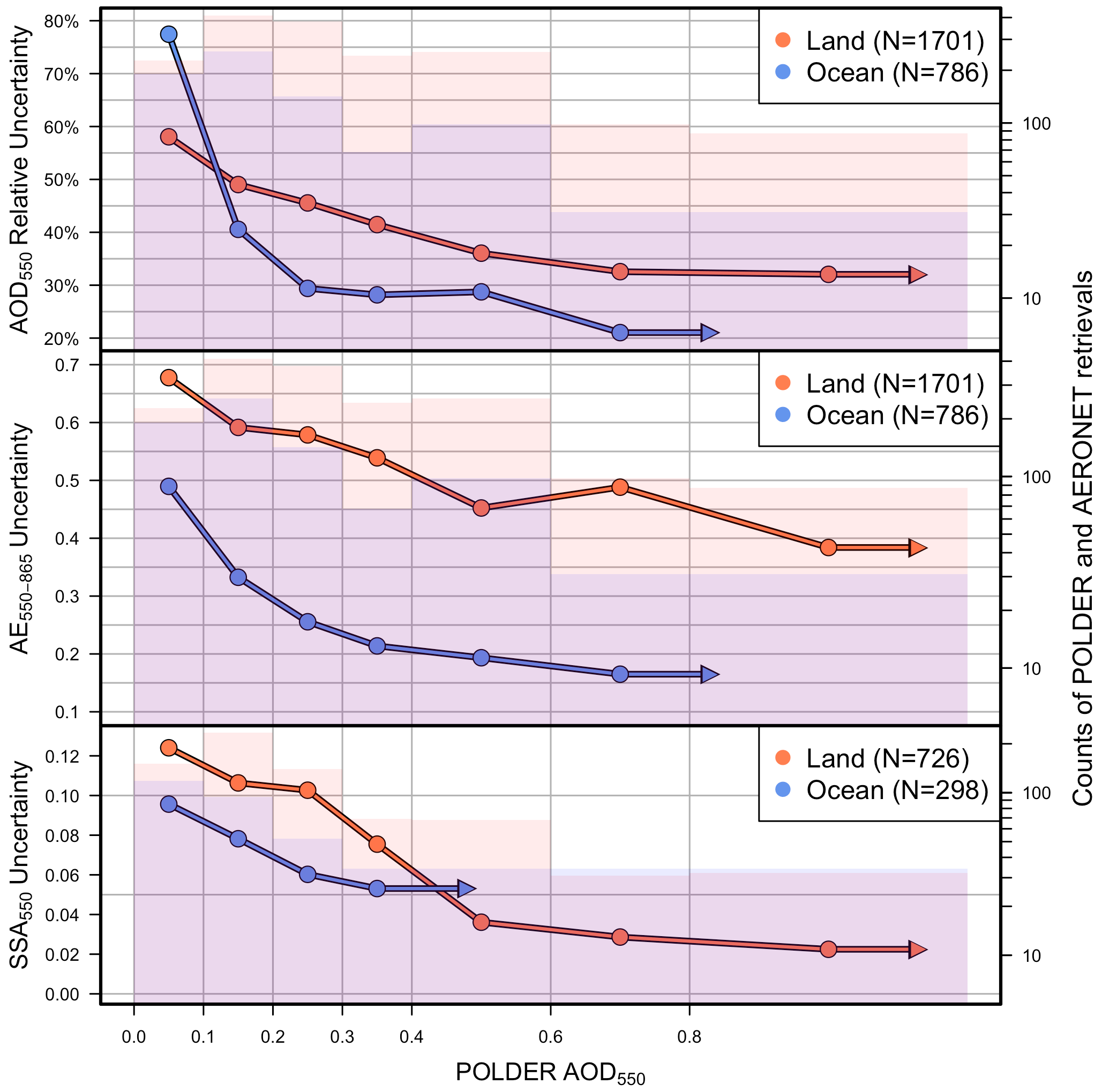
Figure A1 POLDER SRON product uncertainty in AOD₅₅₀, AE_550–865 and SSA₅₅₀ based on an AERONET evaluation for several POLDER AOD₅₅₀ bins. Red and blue lines depict the uncertainty in the over-land and over-ocean retrievals, respectively (left axis). The respective colored bars illustrate the number of collocated POLDER and AERONET retrievals that were used to calculate the observable uncertainty in each AOD₅₅₀ bin (right axis), and N depicts the total number. Note that only AOD₅₅₀ uncertainty was estimated in relative terms, by dividing by AERONET AOD₅₅₀. The AOD₅₅₀ and AE_550–865 evaluation is based on the AERONET version 3 level 2.0 direct sun algorithm, while the AAOD₅₅₀ and SSA₅₅₀ evaluation is based on the AERONET version 3 level 1.5 direct sun and inversion algorithm.

In addition to the uncertainty in observations presented in Fig. A1, a representation error was added to the uncertainty in AOD₅₅₀ and AE_550–865 observations. Specifically, an analysis was performed using CAMS reanalysis in two resolutions, one in a resolution of 1^∘ × 1^∘ (resolution of POLDER level 3) and one in a coarser resolution of 1.875^∘ × 1.875^∘ (resolution of ECHAM–HAM). The objective of this analysis was to determine how well an observation on a 1^∘ × 1^∘ horizontal resolution represents the respective observations on a 1.875^∘ × 1.875^∘ model resolution. This was done by firstly collocating the data of the two resolutions. Obviously, each coarse resolution paired with multiple high-resolution observations. For each paired observation the differences were calculated. Then the standard deviation of the differences for each 1.875^∘ × 1.875^∘ grid box was estimated. The global mean value of all standard deviations was used as a representation error, distinctively for the AOD₅₅₀ and AE_550–865 case. The added representation error for AOD₅₅₀ is 0.022 and for AE_550–865 is 0.062. The respective values for a coarser resolution (3.75^∘ × 3.75^∘) are 0.045 and 0.120 for AOD₅₅₀ and AE_550–865, respectively. No representation error was used for the observations of SSA₅₅₀, since the SSA was not available in the Atmosphere Monitoring Service (ADS) for the CAMS reanalysis.

Appendix B

The prior emission uncertainties are based on an ensemble of simulations where in each member the emissions of each aerosol species have been distinctively perturbed. The emissions were multiplied with numbers that were sampled from a positive skewed distribution, which had a distinctive standard deviation for each species and a mean of 1. The distinctive standard deviations were based on the standard deviation of the differences between ECHAM–HAM minus POLDER daily AOD. We assumed that the standard deviation of these differences filtered over specific locations can be used as a proxy for emissions uncertainty by species.

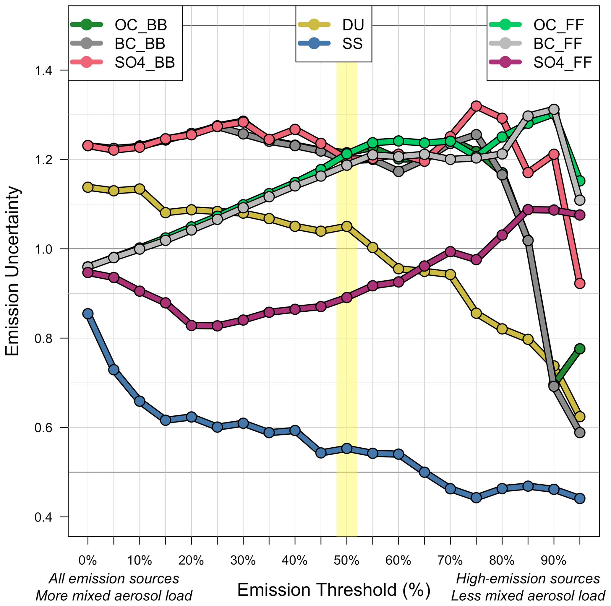
Figure B1 The emission uncertainty as a function of the emission threshold for each parameter. The emission uncertainty (yy^′ axis) is set as the standard deviation of daily AOD₅₅₀ differences of POLDER − ECHAM–HAM for the year 2006. The emission threshold (xx^′ axis) depicts the percentile of daily emissions. The SO₄ emission uncertainty also represents the emission uncertainty used for SO₂ and DMS. Note that for DU, SS and OC multiple modes are perturbed distinctively, but the modes of those species use the same emission uncertainty. The yellow shaded area highlights the emission uncertainty used in this study, where the emission threshold is set at 50 % (includes sources with higher values than the median). For more details, see the text in Appendix B.

In Fig. B1 the estimated emissions uncertainty (standard deviation differences of AOD, explained above) is depicted as a function of several emissions percentiles, where a low percentage contains all the daily grid box emissions and a high percentage contains only the highest daily grid box emissions. Theoretically, when the emissions threshold is high, the contribution of that specific aerosol species to the total aerosol load in the atmosphere increases; thus the emission uncertainty will be more representative of that species.

The current analysis gives little information on the emissions uncertainty over low-emission sources; thus we assume that low- and high-emission sources share the same uncertainty. The emissions uncertainty for this study was based on the median (50 %) emissions threshold in order to filter out cases where multiple aerosol species are mixed in the atmosphere but also to include sources with relative mediocre strength. Note that this approach attributes all modeling errors that may affect aerosol optical properties (e.g., transport, deposition, water uptake, aerosol chemical production) as emissions uncertainty. Consequently, the emissions uncertainty is possibly overestimated in some cases. For example, a previous study has suggested that fossil fuel emissions are lower than 20 % for BC and lower than 42 % for SO₂ (Granier et al., 2011). Further, note that since we are using AOD as a proxy for emissions uncertainty, the absorbing aerosols (BC) will have a similar uncertainty with the scattering aerosol species (OC) that are emitted in the same locations.