Signatures of gravity wave-induced instabilities in balloon lidar soundings of polar mesospheric clouds

The Balloon Lidar Experiment (BOLIDE), which was part of the Polar Mesospheric Cloud Turbulence (PMC Turbo) Balloon Mission has captured vertical profiles of PMCs during a 6 d flight along the Arctic circle in July 2018. The high-resolution soundings (20 m vertical and 10 s temporal resolution) reveal highly structured layers with large gradients in the volume backscatter coefficient. We systematically screen the BOLIDE dataset for small-scale variability by assessing these gradients at high resolution. We find longer tails of the probability density distributions of these gradients compared to a normal distribution, indicating intermittent behaviour. The high occurrence rate of large gradients is assessed in relation to the 15 min averaged layer brightness and the spectral power of short-period (5–62 min) gravity waves based on PMC layer altitude variations. We find that variability on small scales occurs during weak, moderate, and strong gravity wave activity. Layers with below-average brightness are less likely to show small-scale variability in conditions of strong gravity wave activity. We present and discuss the signatures of this small-scale variability, and possibly related dynamical processes, and identify potential cases for future case studies and modelling efforts.

1 Introduction

The intricate small-scale structure of noctilucent or polar mesospheric clouds (PMCs) has been attributed to the action of gravity waves very early on (Witt, 1962). To this day, the strong backscatter of the ice particles that PMC are made of represents a unique opportunity to observe dynamical processes in the upper mesosphere. High-resolution observations of PMC are obtained using both active and passive remote sensing instruments that are based on the ground or carried by satellite, aircraft, or balloon (e.g. Baumgarten and Fritts, 2014; Gao et al., 2018; Miller et al., 2015; Reimuller et al., 2011; Schäfer et al., 2020). Lidar instruments allow for high vertical resolution down to a few metres, revealing various stages in the approach to, or attainment of, gravity wave breaking and other nonlinear dynamics made visible by the PMC layer. However, a comprehensive physical interpretation of the waves and structures inside the PMC layer observed by lidar is limited by the sparseness of the horizontal sampling. Complementary spatial information can be provided by, for example, cameras, but opportunities in terms of time and location for observations from the ground are scarce, as lidars operate best in darkness, but cameras can observe PMC during twilight only. Hence, both camera and lidar instruments have to be operated at significant distance for common-volume observations, and simultaneous observations depend on suitable conditions at two places (Baumgarten et al., 2009). This limitation is overcome by lifting a single payload, including a lidar instrument and cameras, to the upper stratosphere, where the sky is always dark and the view unhindered by tropospheric clouds. This was accomplished first by the Polar Mesospheric Cloud Turbulence (PMC Turbo) Balloon Mission that observed the PMC layer along the Arctic circle during a 6 d flight in July 2018 (Fritts et al., 2019).

The effect of gravity waves and the processes associated with their breaking on the PMC layer is not fully understood to date, in part due to the wide range of scales, the often unknown state of the background atmosphere, and the microphysical evolution of PMC particles in this multiscale environment. Whether stratospheric gravity wave activity influences the occurrence of PMCs, or not, has been answered differently at different locations (Thayer et al., 2003; Innis et al., 2008; Chu et al., 2009). Gravity wave activity based on upper mesospheric radar measurements was not found to be correlated with the occurrence of PMCs at a specific Arctic site (Wilms et al., 2013). However, Chandran et al. (2012) deduced from the global Cloud Imaging and Particle Size (CIPS) dataset that regions of strong gravity wave activity, for both long and short periods, suffer from reduced PMC brightness on average. This finding is supported by a number of modelling studies using microphysical models that showed that gravity waves generally act to destroy PMCs (Jensen and Thomas, 1994; Rapp et al., 2002; Dong et al., 2021). The altitude and temperature variations induced by gravity waves or other small-scale dynamics can result in the rapid sublimation of ice particles. The asymmetry in the growth and sublimation rates ensures that particles are more likely to be destroyed than to grow large enough in size to be observable and that particles, once sufficiently reduced in diameter, are unlikely to regrow to observable sizes for a significant amount of time. The outcome may depend on the period of gravity waves modulating the environment in the vicinity of PMC. Rapp et al. (2002) found a reduction in PMC brightness for short-period gravity waves below 6.5 h only. In three-dimensional simulations, Dong et al. (2021) observed the sublimation of a modelled PMC layer caused by breaking gravity waves within 30 min, leading to the formation of holes (or voids) which resemble structures observed in PMC satellite images (Thurairajah et al., 2013). At timescales of minutes, the PMC layer can generally be considered a passive tracer of the dynamic processes (Fritts et al., 1993; Dong et al., 2021). Lidar measurements of the changes in volume backscatter coefficient, also termed PMC brightness, are at these scales therefore predominantly due to changes in density and not changes in particle size. As visual PMCs frequently display small-scale structures attributed to gravity waves and processes associated with their breaking, high-resolution observations of the PMC layer are ideally suited to studying the statistics and pathways of energy transfer from gravity waves down to turbulent scales (Warhaft, 2000; Shraiman and Siggia, 2000).

Among the millions of images acquired during the PMC Turbo mission were intriguing displays of small-scale vortex rings (Geach et al., 2020), Kelvin–Helmholtz instabilities (Kjellstrand et al., 2022), and mesospheric bores (Fritts et al., 2020). The selection of these events was mainly based on the interpretation of the images that were post-processed to enhance small-scale structures (Kjellstrand et al., 2020), and they make up only the tip of an iceberg of potentially interesting observations. Colocated lidar data have, in all cases, revealed significant small-scale structures with signatures that are likely inherent to the dynamic processes studied. To foster further analysis and interpretation of this dataset and others, we here aim to provide statistics and a systematic review of such patterns. We will employ a general, easy-to-implement method for identifying features related to quick changes in the volume backscatter coefficient or PMC brightness on scales of 40 m and 20 s that represent processes related to dynamical instabilities following the breaking of gravity waves. The results can be used to select promising subsets of the PMC Turbo dataset for subsequent case studies, aid the interpretation of similar signatures in other lidar datasets, and serve as a reference for future modelling of the effect of gravity waves on PMC layers. As stated by Fritts et al. (2019), such observations have the potential to confirm or constrain modelling results or discover processes that are as yet unknown. In addition, we present a statistical analysis of the occurrences of such patterns with regard to ambient conditions. Gravity wave activity and layer brightness can be derived from the lidar data and thus provide the chance to relate the occurrence of small-scale structures that are related to gravity wave (GW) breaking or other nonlinear dynamics, to the strength of short-period gravity wave activity, and to the mean layer brightness. The intention is to find out whether the studied events arise during periods of intense gravity wave activity or rather during quiet times and whether this goes along with enhanced or reduced PMC brightness. This study thus also aims to complement the modelling study of Dong et al. (2021) with a comprehensive observational dataset. The step beyond previous analysis of observational data is rooted in the high temporal and spatial resolution of the PMC Turbo lidar dataset that facilitates the detection of turbulent-like features and instabilities that arise as an effect of breaking gravity waves. Intentionally, we focus this study on the PMC lidar dataset of PMC Turbo and will make use of the associated images in subsequent case studies identified by this work.

2 Method

2.1 Instrument and data

The Balloon Lidar Experiment (BOLIDE) is a Rayleigh backscatter lidar designed to operate on board a stratospheric long-duration balloon at an altitude of ∼40 km at polar latitudes (Kaifler et al., 2020). During the 6 d flight of PMC Turbo along the Arctic circle from Sweden to Canada in July 2018, almost 50 h of high-resolution PMC soundings were recorded (Kaifler et al., 2022; Fritts et al., 2019). PMCs are detected relative to a standard atmosphere density profile, as described in detail by Kaifler et al. (2022). In short, the atmospheric return signal from the 28^∘ off-zenith tilted 4.2 W laser beam was collected by a 0.5 m diameter receiving telescope and detected by an avalanche photodiode operated in a single-photon counting mode. The resulting photon signals were time stamped with nanosecond resolution, allowing for flexible choices in binning the lidar data in the time and range during postprocessing. In data analysis, the measurements obtained along the line of sight of the laser beam are corrected for background and range, converted to altitude, and normalized to a standard density profile. The resulting relevant physical quantity is the volume backscatter coefficient β, a measure for PMC brightness influenced by both the size and number density of ice particles within the observed volume. This work makes use of lidar data at 20 m vertical and 10 s temporal resolution. Although higher resolutions are possible during bright displays with a high signal-to-noise ratio, these parameters are a suitable choice for the type of analysis carried out in this study. We include values of β that are 2.5 standard deviations above the background and discard profiles where the vertical sum of ln β in units of 10⁻¹⁰ m⁻¹ sr⁻¹ is below a threshold value of 30. The intention is to reject sporadic detections with low significance that cannot be attributed to a coherent PMC layer. The threshold is chosen such that the estimate of the mean layer altitude is sufficiently smooth for the subsequent spectral analysis. In total, 41.9 h of PMC detections remain for the analysis.

2.2 Gradients in high-resolution data

Volume backscatter coefficients of PMCs, β, follow an exponential distribution (Berger et al., 2019; Kaifler et al., 2022). It is therefore convenient to plot and analyse β on a logarithmic scale. On a linear scale, large β dominate, and the details of the variations at smaller β are lost. As a measure for small-scale variability, we evaluate the gradients $\partial /\partial z\ln \mathit{\beta }$ and $\partial /\partial t\ln \mathit{\beta }$, abbreviated as ∂_zβ and ∂_tβ, in altitude z and time t. Gradients are widely used in data analysis, e.g. in the analysis of the topographic lidar data of complex terrain for the derivation of high-resolution digital elevation models (Szypuła, 2019). We compute the derivatives using a three-point (quadratic) Lagrangian interpolation at a resolution of 20 m and 10 s. Large values of ∂_zβ indicate distinct layer edges and highlight thin and bright multiple layers. Moving from low to high altitudes, positive (negative) values of ∂_zβ mark lower (upper) layer boundaries. Large values of ∂_tβ contrast the vertical motions of the PMC layers, presumably induced by vertical winds, or spatial patterns that are horizontally advected through the lidar field of view. We will later select large absolute values of ∂_zβ and ∂_tβ to identify periods with intense small-scale variability.

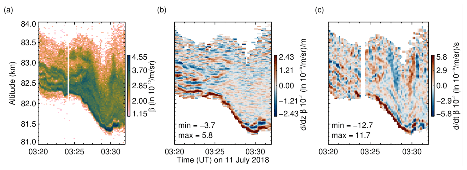
Figure 1 (a) Volume backscatter coefficients β between 03:20 and 03:35 UT on 11 July 2018. (b) Gradients in altitude, highlighting vertically stacked layers before 03:27 UT. (c) Gradients in time, clearly showing the quick descent and the following ascent of the PMC layer around 03:29 UT. The resolution of the data analysed and shown in panel (a) is 20 m and 10 s, and the gradients shown in panels (b) and (c) have been smoothed to 40 m and 20 s, respectively.

We illustrate the application of the gradient analysis in both dimensions with an event observed on 11 July between 03:20 and 03:33 UT. We will show later that this particular event exhibits the largest gradients in the PMC Turbo BOLIDE dataset. Figure 1 shows volume backscatter coefficients, as measured by the lidar as a function of altitude and time, and both the vertical and temporal gradients. To enhance the visibility of the plots, we smooth the gradients between adjacent profiles, i.e. to 20 s for ∂_zβ and to 40 m for ∂_tβ. At 03:20 UT, a wide layer above 82 km altitude with a pronounced internal structure including at least four narrow, closely spaced sublayers below 100 m width are observed. At 03:26 UT, a sudden, steep descent of the PMC layer occurs. The lower boundary that descends by 1 km from 82.2 to 81.2 km, is of both very large β and very large ∂_zβ. Best visible in Fig. 1c, the upper boundary is subjected to a similar downward motion, yet it starts 3 min later and descends quicker and deeper (area with blue colour). A corresponding increase in layer altitude follows shortly after (red colour at 03:30 UT). At the minimum altitude at 03:30 UT, the layer brightness quickly increases to $\mathit{\beta }=\mathrm{4.37}\times \ln {\mathrm{10}}^{-\mathrm{10}}$ m⁻¹ sr⁻¹ for a duration of 1 min. This goes along with large gradients of ${\partial }_z\mathit{\beta }=\mathrm{5.8}\times {\mathrm{10}}^{-\mathrm{2}}\ln ({\mathrm{10}}^{-\mathrm{10}}$ m⁻¹ sr⁻¹) m⁻¹ and ${\partial }_t\mathit{\beta }=-\mathrm{12.7}\times {\mathrm{10}}^{-\mathrm{2}}\ln ({\mathrm{10}}^{-\mathrm{10}}$ m⁻¹ sr⁻¹) s⁻¹.

2.3 Background environment

To define a proxy for gravity wave activity, we follow Geach et al. (2020), who studied vortex rings of ≈5 km diameter generated by the breaking of a short-period gravity wave. Its signature in lidar data proved to be sinusoidal oscillations of the PMC layer with a period of 670 s. Based on this result, we construct a proxy P_GW for wave activity from the PMC layer altitude variations. We start with the time series of the ln β-weighted mean PMC layer altitude z_c that is filled with linear interpolations at times of either below-threshold or no PMC detections. z_c is then spectrally decomposed using Morlet wavelets, which are now widely used in the analysis of atmospheric data and are considered an optimal choice regarding the periodicity and localization of wave structures in PMCs (e.g. Rong et al., 2018). We focus on short-period gravity waves above the buoyancy frequency of about 5 min by selecting the spectral range of a 5–62 min period. P_GW is then finally determined as the averaged spectral power within this band. It is inherently smoothed by the wavelet analysis and can thus be used as a representation of the gravity wave background.

Figure 2 (a) Volume backscatter coefficients of the PMC layer on 11 July 2018 at 02:20–06:30 UT. (b) PMC layer altitude z_c (black) and altitude variations reconstructed from a range of filtered scales corresponding to periods between 5 and 62 min (blue). (c) Scale-averaged spectral power P_GW within a 5–62 min period as a proxy for short-period gravity wave activity. (d) The 15 min smoothed, vertically integrated brightness P_β as a proxy for background PMC layer brightness.

As a proxy P_β for the mean PMC layer brightness, we employ vertically integrated volume backscatter coefficients smoothed by a 15 min running mean. The vertical integration facilitates comparisons with camera and visual observations, which observe accumulated brightness along the line of sight and are insensitive to the effects of convergence; for example, a wide, dim layer has the same integrated brightness as a thin, bright layer. The smoothing to a lower resolution effectively removes the brightness variations at scales below 15 min and thus separates this quantity from the small-scale variability assessed by the gradient analysis. As a consequence of the vertical integration and temporal smoothing, as with P_GW, the number of independent data points in P_β is reduced compared to the gradients evaluated on high-resolution data. For an illustration of P_GW and P_β, we show a larger part of the PMCs observed on 11 July 2018, including the part at around 03:30 UT that we selected to demonstrate the gradient analysis in the previous section (Fig. 2a). The mean PMC altitude z_c (Fig. 2b; black curve) is a good proxy for the layer altitude, and the filtered time series effectively captures the part of the motion in the desired range, excluding both the scale of a few hours and the minute-scale perturbations, such that it is a good representation of the gravity wave activity we seek to characterize (Fig. 2b; blue curve). P_GW is maximum at 04:00 UT due to the change in altitude of almost 2 km in the selected spectral band (Fig. 2c). Maxima in P_β are found at around 05:10 and 06:00 UT when the layer is locally bright or wide (Fig. 2).

Figure 3 Probability density function of (a) vertical brightness gradients ∂_zβ and (b) temporal brightness gradients ∂_tβ. The solid line shows the distribution of all values normalized to unity. The dotted lines show the Gaussian distribution of the same mean and standard deviation. The dashed line shows the maximum of the absolute gradient value per profile. The vertical lines are drawn at ±2σ and include 94.7 % of all values. (c) Percentage of PMC values (black line) and profiles (dashed line) with $\left|{\partial }_z\mathit{\beta }\right|>l{\mathit{\sigma }}_z$ or $\left|{\partial }_t\mathit{\beta }\right|>l{\mathit{\sigma }}_t$, depending on the threshold l, where l=2 is again marked. In total, 9.7 % of all gradient values are above 2σ, and 96.6 % of all PMC profiles contain gradients of either $\left|{\partial }_z\mathit{\beta }\right|>\mathrm{2}{\mathit{\sigma }}_z$ or $\left|{\partial }_t\mathit{\beta }\right|>\mathrm{2}{\mathit{\sigma }}_t$.

3 Results

At a resolution of 20 m and 10 s, the BOLIDE dataset includes 1.06×10⁶ independent measurements with sufficient signal-to-noise ratio of PMC volume backscatter coefficient. A total of 672 921 values have neighbours that allow for the calculation of both gradients ∂_zβ and ∂_tβ. They occur within 13 255 independent vertical profiles totalling 36.8 h. Figure 3a and b show normalized probability density functions of all gradients ∂_tβ and ∂_zβ derived from measured data. The distributions have approximately zero mean and extend to ${\partial }_z\mathit{\beta }=\mathrm{6.0}\times {\mathrm{10}}^{-\mathrm{2}}\ln ({\mathrm{10}}^{-\mathrm{10}}$ m⁻¹ sr⁻¹) m⁻¹ and ${\partial }_t\mathit{\beta }=\mathrm{13.4}\times {\mathrm{10}}^{-\mathrm{2}}\ln ({\mathrm{10}}^{-\mathrm{10}}$ m⁻¹ sr⁻¹) s⁻¹. Gradients of this magnitude mean that the brightest local PMC volume of $\mathrm{4.67}\times \ln {\mathrm{10}}^{-\mathrm{10}}$ m⁻¹ sr⁻¹ can potentially emerge from or fade within $\mathrm{4.67}/\mathrm{0.060}=\mathrm{78}$ m in the vertical or $\mathrm{4.67}/\mathrm{0.134}=\mathrm{35}$ s in time. The maximum gradient value is thus close to the limits given by the resolution and smoothing of the gradients.

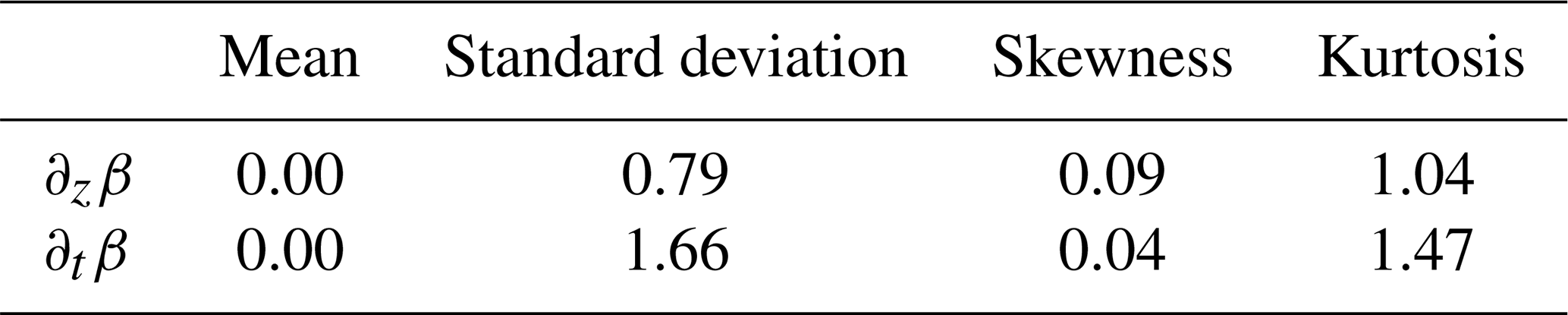
The moments of the distributions of ∂_zβ and ∂_tβ are listed in Table 1. The standard deviations are ${\mathit{\sigma }}_z=\mathrm{0.79}\times {\mathrm{10}}^{-\mathrm{2}}\ln ({\mathrm{10}}^{-\mathrm{10}}$ m⁻¹ sr⁻¹) m⁻¹ and ${\mathit{\sigma }}_t=\mathrm{1.66}\times {\mathrm{10}}^{-\mathrm{2}}\ln ({\mathrm{10}}^{-\mathrm{10}}$ m⁻¹ sr⁻¹) s⁻¹, respectively. The distributions are skewed to positive values, especially ∂_zβ. This indicates the steeper lower boundaries of the PMC layers or respective sublayers compared to top boundaries. The kurtosis is positive, meaning that the distributions have longer tails than the normal distribution. For comparison, we plot the Gaussian distributions with the same mean and standard deviations in Fig. 3a and b as dotted lines. This is an indication of intermittent behaviour.

To further characterize the distributions of ∂_zβ and ∂_tβ with regard to the occurrence of large gradients, we shift a threshold lσ, with σ being the standard deviation of the dataset, and l=0…5. l=2 is marked by vertical lines in Fig. 3a and b, as an example. For l=2, 5.3 % of the ∂_zβ (∂_tβ) values are found in the tail of the respective distribution (Fig. 3a and b), while 9.7 % of all PMC detections exhibit gradients that are within the tail of either distribution. The latter quantity is shown in Fig. 3c as a function of l as a solid curve. The dashed curve shows the percentage of the vertical profile that exhibits gradients within the tail of either distribution. The result that 9.7 % of all gradients that are found in the tails for l=2 are actually distributed across 96.6 % of vertical profiles means that large gradients occur frequently and that smooth and unperturbed PMC layers are rare.

Table 1 Statistical moments of ∂_zβ in units of ${\mathrm{10}}^{-\mathrm{2}}\ln ({\mathrm{10}}^{-\mathrm{10}}$ m⁻¹ sr⁻¹) m⁻¹ and ∂_tβ in units of ${\mathrm{10}}^{-\mathrm{2}}\ln ({\mathrm{10}}^{-\mathrm{10}}$ m⁻¹ sr⁻¹) s⁻¹. A raw kurtosis of 3 that is expected for a Gaussian distribution was subtracted.

The mean P_GW of all the PMC observations within the BOLIDE dataset is 0.76±0.77ln  km², corresponding to a PMC layer altitude variability of $\sqrt{\exp \left(\mathrm{0.76}\right)}=\mathrm{1.46}$ km in the 5–62 min spectral band. The minimum value is −2.1 and corresponds to a variability of 350 m, while the maximum value is 2.26 with a variability of 3.1 km. The mean P_β is $\mathrm{0.29}\pm \mathrm{0.18}\ln {\mathrm{10}}^{-\mathrm{6}}$ sr⁻¹ and values range between 0.02 and $\mathrm{0.96}\times \ln {\mathrm{10}}^{-\mathrm{6}}$ sr⁻¹. We divide the PMC profiles into four categories relative to these mean values $\stackrel{\mathrm{‾}}{P_{\text{GW}}}$ and $\stackrel{\mathrm{‾}}{P_{\mathit{\beta }}}$ in order to assess the occurrence rate of large gradients in brighter or dimmer PMC layers exposed to weak or strong gravity wave activity. The selection criteria are defined in Table 2. Though desirable, a finer division is not implemented because of the limited number of independent values due to the smoothing of P_GW and P_β. The fractions of gradient values per category as a function of the threshold l are shown in Fig. 4, where, again, all profiles are included on the left for l=0, and on the right, only those with larger gradients in either ∂_tβ or ∂_zβ remain. We find that dimmer layers with strong gravity wave activity (category B in Fig. 4) are most common, followed by brighter layers with strong gravity wave activity (category D). As the statistics are narrowed to the largest-gradient profiles, category D layers make up the largest share. The PMC layers belonging to the most common category (B) are, however, unlikely to exhibit large gradients compared to layers of the other categories.

Table 2 Criteria for classification of PMC layers (dim or bright and strong or weak gravity wave activity, according to $\stackrel{\mathrm{‾}}{P_{\mathit{\beta }}}$ and $\stackrel{\mathrm{‾}}{P_{\mathrm{GW}}}$).

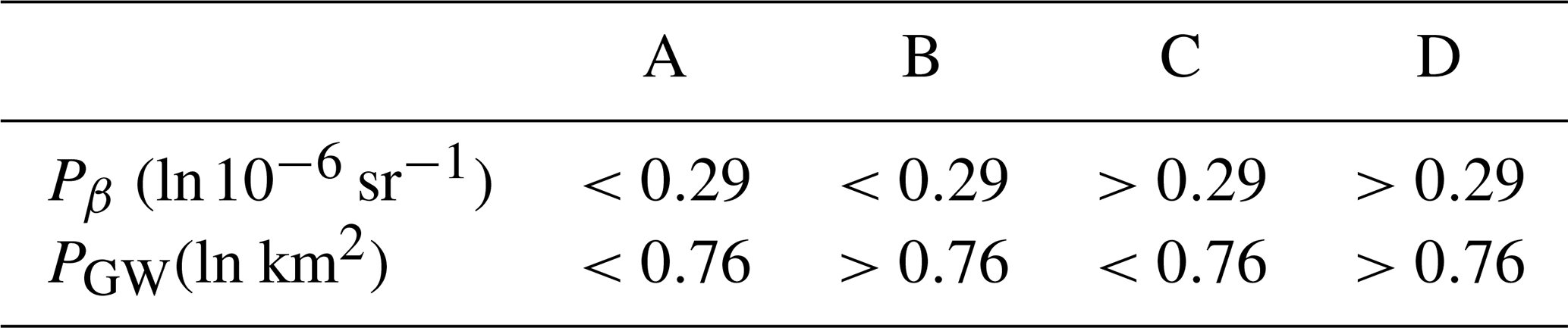
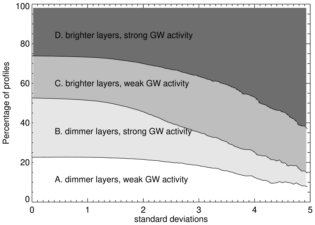
Figure 4 Percentage of PMC profiles with gradients $\left|{\partial }_z\mathit{\beta }\right|>l{\mathit{\sigma }}_z$ or $\left|{\partial }_t\mathit{\beta }\right|>l{\mathit{\sigma }}_z$ for the four categories defined in Table 2. For l=0, all PMC profiles are included, while at larger values of l, only profiles that exhibit increasingly larger gradients are considered.

In the next section, we will look into the morphology of the layers that exhibit large gradients. We will first discuss the already published cases in the light of our results and then proceed to describe four general groups of PMC layer sections based on their morphology and discuss their link to the dynamical processes that led to their formation.

4 Discussion

The PMC layer sections that contain mostly PMC profiles with gradients larger than 2σ exhibit all types of small-scale variability, including vertical, oscillatory motions of bright, thin layers, the internal structure of wider layers, multiple layers, and vertical displacements of PMC layers. Both large and small displacements are included. Although more sophisticated methods could be developed to detect those signatures, we deem the gradient analysis a suitable choice. It is an easy-to-implement and general method that is not tailored to specific patterns and is thus suitable for the detection of signatures of potentially previously unknown dynamics. We refrained from the application of wavelets, either one- or two-dimensional, to assess the small-scale variability in PMC as we did not want to make the assumption of an underlying periodicity but rather to allow for singular or irregular structures within the PMC layer at the smallest scales.

Geach et al. (2020)Kjellstrand et al. (2022)Fritts et al. (2020)

Table 3 PMC layer category and percentage of PMC detections or profiles with large gradients for the periods of nine major PMC events defined by Fritts et al. (2019, their Table 2). For reference, the dataset mean percentage of PMC detections with gradients above the 2σ threshold is 9.8 %, and for PMC profiles with gradients above the 4σ threshold, it is 9.9 % (from Fig. 3c).

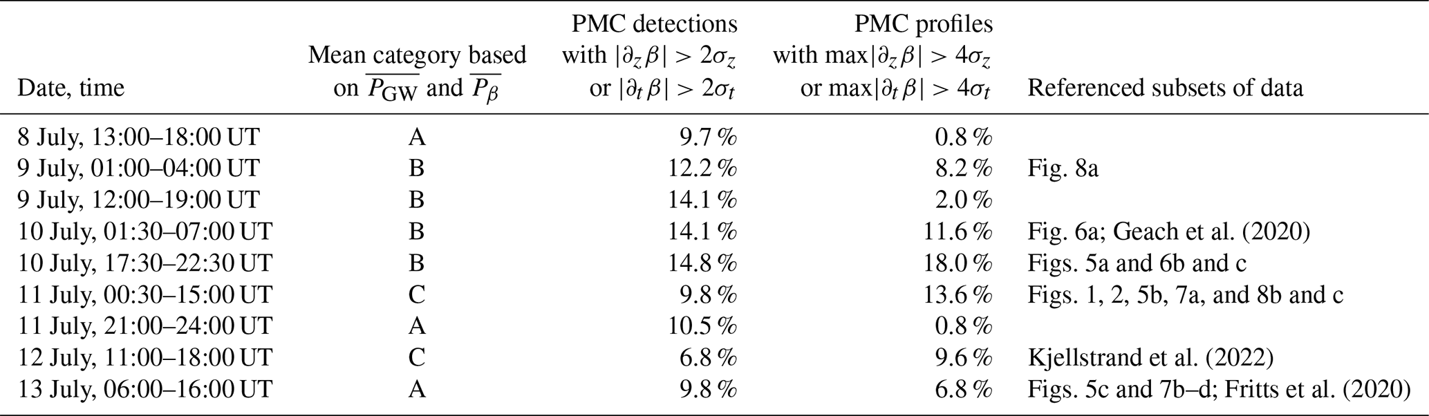
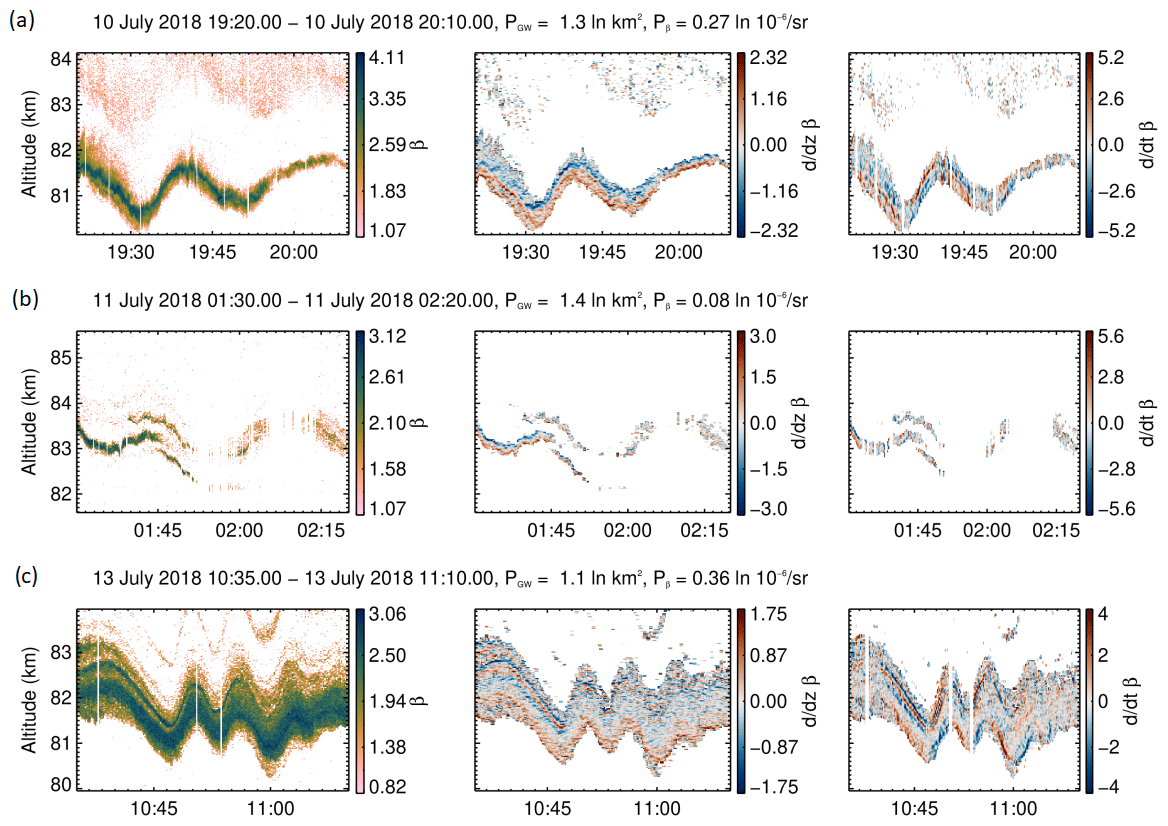
Figure 5 Examples of PMC layers with largely sinusoidal oscillations in altitude. The title line gives the start and end dates in addition to the mean P_β and P_GW for this duration. The colour scale includes the minimum and maximum of β in units of ln 10⁻¹⁰ m⁻¹ sr⁻¹ and 2 standard deviations of the gradient values (units of ${\mathrm{10}}^{-\mathrm{2}}\ln ({\mathrm{10}}^{-\mathrm{10}}$ m⁻¹ sr⁻¹) m⁻¹ and ${\mathrm{10}}^{-\mathrm{2}}\ln ({\mathrm{10}}^{-\mathrm{10}}$ m⁻¹ sr⁻¹) s⁻¹). All vertical axes extend 4.5 km in altitude and are centred around the mean z_c.

An evaluation of the statistics of the gradients, in particular Fig. 3c, has established that gradients larger than 2σ are widespread whenever PMC is present. This is in agreement with the visual impression from both ground-based observations and the PMC Turbo images of highly variable PMC layers at small spatial scales. Fritts et al. (2019) divided the PMC Turbo dataset into eight major PMC events, gave an initial assessment of the relevant dynamics and likely impact, and stated the magnitude of the forcing and the occurrences of gravity wave breaking, fronts, or bores and Kelvin–Helmholtz instabilities. In Table 3, we complement this list with the results of our analysis, including an approximate category based on P_GW and P_β averaged over the time period listed and percentages of PMC detections and PMC profiles in the tails as shown in Fig. 3c. The assessment by Fritts et al. (2019) of weak, moderate, or strong dynamics or forcing is reflected in our result for the category, in the way that mostly weak dynamics or forcing relates to categories A and C, and stronger dynamics and forcing to categories B and D. The events that stood out in the initial visual inspections of PMC Turbo images and lidar data, some of which have already been analysed for their dynamics, all show increased and, in most cases, even very large gradients. The small-scale vortex rings studied by Geach et al. (2020) were observed on 10 July 2018 between 02:30–02:57 UT. Their signature includes a rapid (1 min period) downward extension of comparably weak PMC backscatter by almost 1 km from the lower PMC boundary. The upper boundary, in contrast, was clearly defined and constant in altitude. This resulted in a large vertical gradient ∂_zβ of $\mathrm{4.4}\times {\mathrm{10}}^{-\mathrm{2}}\ln ({\mathrm{10}}^{-\mathrm{10}}$ m⁻¹ sr⁻¹) m⁻¹ at the top boundary, and the variation in the lower boundary is clearly reflected in quick successions of positive and negative values of ∂_tβ amounting to $\pm \mathrm{9.6}\times {\mathrm{10}}^{-\mathrm{2}}\ln ({\mathrm{10}}^{-\mathrm{10}}$ m⁻¹ sr⁻¹) s⁻¹. This case was the only occurrence of small-scale vortex rings located at the lower PMC boundary at this level of clarity during PMC Turbo. Rapid oscillations in ∂_tβ at the top boundary or within the layer were also observed on 10 July 2018 at 03:17 UT and 11 July 2018 at 09:20 UT (not shown here). Also characterized by rapid changes in the temporal evolution are the Kelvin–Helmholtz instabilities that occurred on 12 July at 13:30 UT that were studied in detail by Kjellstrand et al. (2022). During this event, vertical displacements affect the whole PMC layer, including multiple narrow sublayers and a sharp lower boundary. The induced absolute gradients amount to $\mathrm{4.5}\times {\mathrm{10}}^{-\mathrm{2}}\ln ({\mathrm{10}}^{-\mathrm{10}}$ m⁻¹ sr⁻¹) m⁻¹ and $\mathrm{11.3}\times {\mathrm{10}}^{-\mathrm{2}}\ln ({\mathrm{10}}^{-\mathrm{10}}$ m⁻¹ sr⁻¹) s⁻¹ and are thus among the largest observed. Similar signatures are visible in the aftermath of this specific event until 12 July 14:20 UT and also on 10 July between 18:45–19:20 UT, on 11 July between 03:55–06:00 UT (compare Fig. 8c), and on 11 July at 13:30 UT (not shown). Looking at the remaining dataset of PMC profiles with large gradients, the patterns can be associated with one or more of the following four groups.

Figure 6 Selected PMC backscatter profiles which are indicative of gravity wave breaking in response to steepening of gravity waves. Same format as in Fig. 5.

• 1.

  PMC layers with largely sinusoidal undulations in altitude. The selected examples shown in Fig. 5 show undulations with periods between 5 and 30 min and are thus likely induced by linear, short-period gravity waves. For the observation shown in Fig. 5a, corresponding PMC Turbo images have confirmed a linear gravity wave of 20 min period and ≈50 m s⁻¹ phase speed. Also, P_GW is well above its mean, putting these layers in category B or D. These types of PMC layers have sharp boundaries, often at the lower edge, and thus vertical gradients are large where the layers emerge from or fade into the background. This is seen, for example, in ∂_zβ on 10 July 2018 at 19:20–20:10 UT (Fig. 5a). Because of the oscillatory motions of these layers, large temporal gradients are also induced, e.g. on 13 July 2018 10:25–11:05 UT (Fig. 5c). But a closer look reveals that those PMC layers are not smooth at smaller scales. Superposed to the larger-scale linear oscillation are small-scale perturbations at timescales of 1–2 min, which result in the detection of large gradients, e.g. around 19:40 UT on 10 July 2018 (Fig. 5a) and at 01:35 UT on 11 July 2018 (Fig. 5b). The PMC Turbo images for Fig. 5a, for example, show evidence for large- and small-scale vortex rings, embedded local instabilities, and multiscale breaking (Fritts et al., 2019, their Fig. 11b). The example on 13 July 2018 (Fig. 5c) highlights another common feature with very narrow-spaced (100 m or less), well-defined sublayers visible 10:35–10:48 UT. The brightest sublayer, starting at 82.6 km, can be traced over several gravity wave periods until around 11:00 UT, when it appears to dissolve. As in all of the examples in Fig. 5, multiple layers exist, with an interlayer spacing between 100 m and 2 km.

Figure 7 PMC layers showing bore-like responses during periods with weak gravity wave activity. Same format as Fig. 5.

• 2.

  PMC layers indicating gravity wave breaking in response to gravity wave steepening. Examples of these very variable layer types are shown in Fig. 6. In these cases, the amplitude of an undulation increases, and the period shortens. This is followed by a reduction in PMC brightness and/or the emergence of small-scale structures. For example, around 05:33 UT on 10 July 2018 (Fig. 6a), a PMC layer perturbed by a large-amplitude gravity wave that is reduced to 10 min period experiences a quick descent with a peak-to-peak amplitude of almost 3 km and β values distributed over a wide range down to the detection limit, likely caused by complex instability dynamics. Interestingly, the situation seems analogous but is mirrored in time at around 05:48 UT except that here a double layer is affected. For a full interpretation of such cases, knowledge of the gravity wave propagation directions and wind speeds relative to the lidar beam path across the PMC layer and the 2-dimensional imaging of PMC structures is very helpful. This information can be deduced from the PMC Turbo images that will be available from NASA's Space Physics Data Facility (or on request). Nevertheless, this lidar observation seems to confirm theoretical results predicting that very strong gravity wave activity inducing large displacements significantly reduces PMC brightness close to or below the detection threshold (Dong et al., 2021). The time frame on 10 July between 17:45 and 19:00 UT is another example of a strong PMC layer modulated by a 10–30 min period gravity wave that causes a multitude of strong instabilities including cusps, linked rings, and herringbone structures (see Fig. 11b in Fritts et al., 2019, at 18:15 UT, and their discussion). The examples featured in Fig. 6 have the largest P_GW in the PMC Turbo dataset.

Figure 8 Multilayered PMC structures experiencing a break up or mixing. Same format as in Fig. 5.

• 3.

  PMC layers that show transitions from weak or no gravity wave activity to major bore-like responses during a few minutes or tens of minutes. These types of layers suggest a rapid evolution or rapid advection of the leading edge of a nonlinear gravity wave packet. Examples are shown in Fig. 7. At 05:13 UT on 11 July 2018, the core of a PMC layer is both deflected upward and downward by 2 and 1 km, respectively, induced by the passage of a mesospheric bore front. The corresponding imagery reveals such a bore by showing a narrow and bright band that extends several hundreds of kilometres across the camera field of view and moves through the lidar beam at 05:13 UT (not shown). The increase in PMC brightness at the bore front revealed by the images is therefore caused by up- and downdrafts that increase the PMC layer width, hinting that, in this case, the bore altitude coincided with the PMC layer altitude. We selected the subset of data including this observation for a detailed future study that employs the PMC images and derived quantities. The successive mesospheric bores studied by Fritts et al. (2020) also belong to this group. Their signatures include extensions of the PMC layer to lower altitudes (in fact, the lowest altitudes in the BOLIDE dataset), as demonstrated by the observations on 13 July 2018 in Fig. 7b and c. For a duration of few minutes only, the layer spreads to approximately double its width, while the brightness remains about constant, leading to a strong increase in integrated brightness. These bores were accompanied by various and intense leading and trailing instabilities (Fritts et al., 2020). At the times of largest descent, tendrils associated with Kelvin–Helmholtz instabilities extrude from the PMC layer (Fig. 7b). Between 13:20 and 13:35 UT, localized increases in brightness indicate successions of small-scale vortex rings, as deduced from the joint analysis of images and lidar soundings. The observation and identification of small-scale vortex rings in lidar data have first been accomplished by using the BOLIDE lidar dataset.

• 4.

  PMC layers that show the break up and/or mixing of previously multilayered, thin features. This class of events is sometimes accompanied by apparent breaking or overturning events associated with group 2. Examples are shown in Fig. 8. These events are ideal targets for the modelling efforts of the effect of gravity waves on PMC layers, as thin layers can be regarded as reliable tracers of small-scale variability. Layers of group 4 and group 2 make up about 20 % of the BOLIDE dataset (13 h) and conform to the irregular or non-parallel multiple layer categories defined by Schäfer et al. (2020, their category IIIb and IIIcii) that accounted for about 25 % of the Arctic Lidar Observatory for Middle Atmosphere Research (ALOMAR) Rayleigh–Mie–Raman lidar dataset. All other BOLIDE data with profiles showing large gradients can be sorted into categories of short-period height variations in both the narrow and wide layers defined by Schäfer et al. (2020, their category Ib and IIbii).

Our analysis in Fig. 4 showed that large gradients are likely to occur during the conditions of both strong and weak gravity wave activity. Most of the examples featured here belong to categories B or D (large P_GW), but PMC layers associated with low values of P_GW can also show distinct small-scale variability. The case with the lowest value is on 11 July at 10:30–12:30 UT, a moderately bright layer of 1–2 km thickness that contains a variety of internal structures. Although undulations in altitude are small during this period, there are large undulations before and after that were likely induced by a gravity wave with a period larger than 60 min. In conclusion, we observed small-scale variability in the PMC layer in all conditions of weak, moderate, and strong short-period gravity wave activity, and the occurrence of truly unperturbed layers can be regarded as a rare phenomenon. We find that PMC observations with below-threshold gradients are generally associated with wide, dim layers without a discernible inner structure (category IIIa of Schäfer et al., 2020) or well-defined thin layers of low brightness with distinct sinusoidal motions (our category B; category I of Schäfer et al., 2020). An example is a set of very narrow PMC layers with sinusoidal undulations of about 20 min periods, as shown in Fig. 5b. While there are several well-defined stacked layers in the beginning, over time the brightness decreases and gradients become smaller. This behaviour is in agreement with theoretical results showing that, under conditions of gravity wave activity, weak layers are further mixed, and ice particles are likely to sublimate, resulting in volume backscatter coefficients that are below the detection threshold. A comprehensive and general assessment of the effect of short-period gravity waves on the ice particle size and number density is likely difficult to obtain from lidar profiling data alone. Atmospheric dynamics occur in three dimensions, and knowledge of the phase speeds and orientations of the gravity waves relative to the wind speed and direction and thus the transport of ice particles is required for a comprehensive analysis. In particular, the temporal axis we show in this work transforms via the local wind speed and the lidar beam movement across the sky to a spatial axis. Our resolution of 10 s likely relates to few hundred metres in the horizontal domain. The required information can be obtained by future experiments including, for example, coincident and common volume imaging and radar observations.

5 Conclusions

We set out to systematically screen, identify, and characterize small-scale signatures that are likely caused by dynamical instabilities generated by the breaking of gravity waves and other nonlinear processes in PMC Turbo BOLIDE lidar data. The focus of this work was on the smallest scales (at 20 m and 10 s resolution), and we applied an easy-to-implement, general method to our lidar data without presupposing any specific patterns. We presented the statistics of gradients occurring in PMC backscatter data and performed a classification of PMC layers based on gradient thresholds, layer brightness, and gravity wave activity. In accordance with visual observations, we confirmed that smooth, unperturbed PMC layers are rare and that small-scale structures are very common. We found that probability density functions of PMC brightness gradients exhibit longer tails compared to a normal distribution, which is an indication of intermittency. Large gradients in the vertical and temporal/horizontal dimension occur frequently during times with both weak and strong gravity wave activity. We believe that the cases identified and presented in this work, in addition to the quantification of gradients, will be helpful for future modelling of the effects of gravity waves on PMC layers.