Simulations of winter ozone in the Upper Green River basin, Wyoming, using WRF-Chem

In the Upper Green River basin (UGRB) of Wyoming and the Uintah Basin of Utah, strong wintertime ozone (O₃) formation episodes leading to O₃ mixing ratios occasionally exceeding 70 parts per billion (ppb) have been observed over the last 2 decades. Wintertime O₃ events in the UGRB were first observed in 2005 and since then have continued to be observed intermittently when meteorological conditions are favorable, despite significant efforts to reduce emissions from oil and natural gas extraction and production. While O₃ formation has been successfully simulated using observed volatile organic compound (VOC) and nitrogen oxide (NO_x) mixing ratios, successful simulation of these wintertime episodes using emission inventories in a 3-D photochemical model has remained elusive. An accurate 3-D photochemical model driven by an emission inventory is critical to understanding the spatial extent of high-O₃ events and which emission sources have the most impact on O₃ formation. In the winter of 2016/17 (December 2016–March 2017) several high-O₃ events were observed with 1 h mixing ratios exceeding 70 ppb. This study uses the Weather Research and Forecasting model coupled with Chemistry (WRF-Chem) to simulate one of the high-O₃ events observed in the UGRB during March 2017. The WRF-Chem simulations were carried out using the 2014 edition of the Environmental Protection Agency National Emissions Inventory (EPA NEI2014v2), which, unlike previous versions, includes estimates of emissions from non-point oil and gas production sources. Simulations were carried out with two different chemical mechanisms: the Model for Ozone and Related Chemical Tracers (MOZART) and the Regional Atmospheric Chemistry Mechanism (RACM), and the results were compared with data from seven weather and air quality monitoring stations in the UGRB operated by the Wyoming Department of Environmental Quality (WYDEQ). The simulated meteorology compared favorably to observations with regard to temperature inversions, surface temperature, and wind speeds. Notably, because of snow cover present in the basin, the photolysis surface albedo had to be modified to predict O₃ in excess of 70 ppb, although the models were relatively insensitive to the exact photolysis albedo if it was over 0.65. O₃ precursors, i.e., NO_x and VOCs, are predicted similarly in simulations with both chemical mechanisms, but simulated VOC mixing ratios are a factor of 6 or more lower than the observations, while NO_x is also underpredicted but to a lesser degree. Sensitivity simulations revealed that increasing NO_x and VOC emissions to match observations produced slightly more O₃ compared to baseline simulations, but an additional sensitivity simulation with doubled NO_x emissions resulted in a considerable increase in O₃ formation. These results suggest that O₃ formation in the basin is most sensitive to NO_x emissions.

1 Introduction

Tropospheric ozone (O₃) is a secondary pollutant that is harmful to human health, plants, and other animals when at elevated levels (Fuhrer et al., 1997; Ebi and McGregor, 2008). The current 2015 US National Ambient Air Quality Standard (NAAQS) for the 8 h average O₃ mixing ratio is 70 parts per billion (ppb). As of 14 August 2020, the 2015 NAAQS standard for the 8 h average O₃ mixing ratio has been proposed to be retained (EPA, 2020). While below the NAAQS threshold, all hourly occurrences of O₃ mixing ratios greater than or equal to 70 ppb are referred to as O₃ events throughout this paper. In the past decades, there has been a significant increase in wintertime as well as summertime O₃ events in the western US (Cooper et al., 2012).

According to the US Energy Information Administration (EIA), in 2018, Wyoming was the eighth-largest producer of oil and natural gas in the United States, with a majority of the natural gas production coming from the Upper Green River basin (UGRB). Specifically, the UGRB accounts for 60 % of the state's natural gas production and 16 % of its oil production (Wyoming State Geological Survey; WSGS, 2020). As of 2017, there were 5506 total wells (5436 producing wells) in the Jonah and Pinedale fields within the UGRB, a 5.7 % increase in the total and 5.9 % increase in the producing wells in the UGRB compared with those in 2016 (http://pipeline.wyo.gov/FieldReportYear.cfm, last access: 9 September 2020). By September 2020, there has been an 8.8 % increase in the total wells since 2017 and a 14.6 % increase in oil- and gas-producing wells in the UGRB.

The formation of O₃ has traditionally been an urban summertime phenomenon because of the need for strong solar intensity and sufficient volatile organic compounds (VOCs). Elevated mixing ratios of wintertime O₃ in a few rural US basins have been associated with the rapid development of natural gas and oil production fields (Mansfield and Hall, 2013; Edwards et al., 2014; Ahmadov et al., 2015; Field et al., 2015a, b). Such elevated O₃ events can occur in winter under specific meteorological conditions: a snow-covered ground that provides high albedo that increases solar intensity while also preventing solar heating of the ground (Carter and Seinfeld, 2012) and quiescent winds. Combined, these conditions result in a persistent temperature inversion and little horizontal and vertical transport, which provides the conditions needed for the photochemical production and buildup of O₃ (Mansfield and Hall, 2018).

Several studies have been carried out to understand the meteorological and chemical processes leading to high-O₃ wintertime events in western US oil and gas basins. These studies have focused on ground-based observational measurements (Schnell et al., 2009; Oltmans et al., 2014b; Rappenglück et al., 2014; Field et al., 2015b; Lyman and Tran, 2015), aircraft measurements (Oltmans et al., 2014a), statistical models (Mansfield and Hall, 2013), box models (Carter and Seinfeld, 2012; Edwards et al., 2013, 2014), and 3-D photochemical models (Rodriguez et al., 2009; Ahmadov et al., 2015; Matichuk et al., 2017). Most of these studies have focused on the UGRB and Utah's Uintah Basin (UB), and both basins have been identified as regions exceeding the NAAQS (Lyman and Tran, 2015). These studies have shown the principal role played by emissions from oil and natural gas production fields in the formation of wintertime O₃. However, the assessment of wintertime O₃ formation in these regions poses serious challenges because each basin has complex topography and meteorological conditions along with poorly constrained precursor (VOC and nitrogen oxide (NO_x)) emissions. One shortfall of previous studies is that most of them have not utilized an existing emission inventory to model O₃ formation. Rather, these studies have utilized observed atmospheric levels of precursors to model O₃ formation, thus making it difficult to assess how future expansion of production or various emission reductions will affect O₃ formation.

Schnell et al. (2009) summarized the confluence of three major factors for wintertime O₃ formation: (i) the extensive production of oil and natural gas that releases NO_x and VOCs or hydrocarbons (HCs) into the atmosphere, (ii) calm wind conditions, and (iii) high albedo caused by snow accumulation at the surface that leads to a strong temperature inversion. A strong inversion traps O₃ and its precursors near the ground; if the inversion persists for several days, the mixing ratios of O₃ and its precursors increase. The high surface albedo also provides additional shortwave radiation for photochemistry compared to a snow-free landscape.

Some studies have specifically pointed out the importance of deep snow cover or high surface albedo in the formation of wintertime O₃. Oltmans et al. (2014b) and Rappenglück et al. (2014) noted that in March 2011, the UGRB experienced high hourly O₃ mixing ratios exceeding 150 ppb, which was associated with the deepest snow cover of the season. In addition, Oltmans et al. (2014b) also pointed out that for the period with snow coverage on the ground, the sum of incoming and reflected ultraviolet levels was almost 80 % higher than the period with no snow cover, highlighting the impact of fresh snow accumulation during high-O₃ events. Rappenglück et al. (2014) noted a significant increase in the background O₃ mixing ratio from around 40 ppb in January to 60 ppb in March 2011, owing to changes in the meteorological conditions and chemical processes that ultimately affect pollutant levels.

Numerous measurement studies have pointed out the important roles played by topography and both meteorological and chemical processes in the UGRB, leading to different O₃ and precursor mixing ratios within each basin and from year to year. Field et al. (2015b) carried out air quality measurements in the UGRB for two consecutive winters (2011 and 2012) at a site located 5 km southeast of a Wyoming Department of Environmental Quality (WYDEQ) air quality and weather monitoring station (Boulder). They measured O₃, reactive nitrogen compounds, methane (CH₄), total non-methane hydrocarbon (NMHC), carbon monoxide (CO), and other standard meteorological parameters. The ambient NMHC mixing ratios in 2012 were lower than in 2011, which resulted in lower observed mixing ratios of O₃ in 2012. Furthermore, Lyman and Tran (2015) measured O₃ and meteorological parameters at different locations in the UB and observed a negative correlation between the O₃ mixing ratio and station elevation. The stations at higher elevations showed very few O₃ exceedance events compared to those at lower elevation. As mentioned by Schnell et al. (2009), a prolonged inversion period traps O₃ near the basin floor due to low wind speeds and limited vertical transport, hence reducing O₃ mixing ratios at the higher elevations. Additionally, Oltmans et al. (2014a) conducted seven aircraft flights in the UB and found that high O₃ mixing ratios were confined to the shallow inversion layer, namely 300–400 m above the ground.

Mansfield and Hall (2013) used a statistical model to accurately predict O₃ formation, but they noted challenges in extending the findings from one basin to another, as factors such as the thermal inversion and snow cover that play an important role in wintertime O₃ formation vary among basins. They used quadratic regression models to predict the daily O₃ mixing ratios in the UB and UGRB and found that the high-O₃ events in the UB and UGRB occurred primarily in February and March, respectively. However, the most intense inversion periods in both basins occurred in January. For both the UB and UGRB, they concluded that these high-O₃ events were highly sensitive to solar radiation, which intensifies as the year progresses.

Carter and Seinfeld (2012) used a box model to study NO_x-limited and VOC-limited regimes in the UGRB. They found that the mixing ratios of NO, NO₂, and NMHC, as well as $\mathrm{VOC}/{\mathrm{NO}}_x$ ratios, varied both spatially and temporally within the basin. Hence, they suggested that equal attention needs to be given to the geographical distribution of O₃ precursors and the local meteorology. Edwards et al. (2013) utilized the Dynamically Simple Model of Atmospheric Chemical Complexity (DSMACC), a photochemical box model with a very detailed chemical mechanism, to assess the sensitivity of NO_x and VOC along with radical precursors¹ for O₃ production in the UB. Using this model, with input of observed O₃ precursors, they were able to accurately simulate relatively small amounts of O₃ formation in the absence of snow cover in 2013. Furthermore, Edwards et al. (2014) demonstrated that the same model could simulate large amounts of O₃ production in the UB when snow cover was present, and they emphasized the importance of carbonyl photolysis in the radical chemistry.

There have been a few studies that have utilized 3-D photochemical models to simulate high-O₃ events in western US oil and gas basins, though to date there has not been a successful 3-D photochemical modeling study that has simulated high wintertime O₃ in the UGRB. Rodriguez et al. (2009) applied the Comprehensive Air Quality Model with Extensions (CAMx) to assess the impacts of the development of oil and gas fields in the western US on the air quality of various parks and national wilderness areas in the inter-mountain west of the US for 2002. They concluded that the model captured the general trend in O₃ on a monthly scale; however, the model did not capture wintertime O₃ formation events occurring during strong inversions. Ahmadov et al. (2015) used the Weather Research and Forecasting model coupled with Chemistry (WRF-Chem, version 3.5.1) to study wintertime O₃ pollution in the UB. To account for the emissions from the oil and gas sector, they employed two different emission scenarios. The first emission dataset was the US Environmental Protection Agency National Emissions Inventory 2011 version 1 (EPA NEI2011; bottom-up) and the second emission dataset was derived from in situ aircraft and ground-based measurements (top-down). They reported an underestimation of hydrocarbons (CH₄ and other VOCs) and an overestimation of NO_x emissions in the NEI2011 inventory compared to the top-down emission scenario. Ahmadov et al. (2015) found that the model simulation using the bottom-up NEI2011 inventory underestimated the high O₃ mixing ratios observed in the UB and that it was necessary to utilize observed mixing ratios of VOCs and NO_x to successfully simulate observed O₃ mixing ratios. Additionally, Matichuk et al. (2017) used WRF and the Community Multiscale Air Quality (CMAQ) model to study a 10 d high-O₃ event in 2013 in the UB. Similarly to Ahmadov et al. (2015), they also used the NEI2011 emission dataset, but they found that the CMAQ model did not reproduce the observed O₃, NO_x, and VOC levels in the UB. Furthermore, Matichuk et al. (2017) identified a positive temperature bias and overestimation of the daytime planetary boundary layer height in the WRF simulations, which was hypothesized to be the reason for the underestimation of O₃, NO_x, and VOCs in the CMAQ model.

As outlined above, wintertime O₃ production requires a thermal inversion as well as sufficiently deep snow (i.e., deep enough to cover most of the vegetation) over a larger area; hence, not all winters experience high O₃ mixing ratios. Additionally, reported emissions from oil and gas have been significantly reduced over the last decade (WYDEQ, 2018). In the winter of 2005 and 2006, the newly installed WYDEQ monitoring stations at Boulder, Daniel South, and Jonah observed multiple occurrences of high O₃ mixing ratios that exceeded the existing 8 h O₃ standard of 1997 (84 ppb; WYDEQ, 2018). Since 2005, WYDEQ has operated regular annual O₃ monitoring in the UGRB, and several air quality and weather monitoring stations have been added in the basin. In recent years (most notably 2008, 2011, 2017, 2019, and 2020), elevated wintertime O₃ events have been observed in the UGRB, with hourly O₃ mixing ratios exceeding 70 ppb for several days in each year. The formation and occurrence of elevated wintertime O₃ mixing ratios comprised an unusual event compared to their urban summertime formation. In July 2012, the UGRB was declared a marginal non-attainment area for O₃ by the US EPA (Rappenglück et al., 2014). In the winter of 2012, there was only 3 d in which the 8 h averaged O₃ mixing ratios exceeded 75 ppb (NAAQS 2008), while in the winter of 2011, there was 7 d of exceedance (Field et al., 2015b) at a site located near the Boulder station. Moreover, in March 2017, the Boulder station observed several hours of an hourly averaged O₃ mixing ratio exceeding 70 ppb (NAAQS 2015).

Given the continued occurrence of high-O₃ events in the UGRB, the lack of modeling studies aimed at understanding the formation of O₃ in the basin, and plans to continue development of the basin, it is important to develop a photochemical model capable of reproducing high-O₃ events of the recent past in order to understand how these events can be prevented in the future. The main goal in this study is to assess if a photochemical model (particularly WRF-Chem) operating with NEI emissions can simulate wintertime O₃ formation in the UGRB. Successful simulation of O₃ events would mean the model could then be utilized to assess effective emission control in preventing future O₃ events as well as the impact of future development on O₃ formation. This study primarily focuses on one of the elevated wintertime O₃ events in the winter of 2017 (a 4 d period from 3 to 7 March 2017) because 2017 was an active year for elevated O₃ in the UGRB (WYDEQ, 2018). The observed hourly O₃ mixing ratios during the period exceeded 70 ppb (NAAQS 2015) for several hours at multiple air quality monitoring stations in the UGRB. In this paper, the results from WRF-Chem simulations for the given period are analyzed, with the aim to understand the production of O₃ in the UGRB.

2 Methods

This section describes the study area, model setup, datasets, methods, and preprocessing tools utilized in the WRF-Chem simulations and to validate the model results.

2.1 Study region

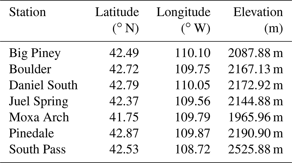
The focus area of this study is the UGRB. The UGRB is a valley located in Sublette County in western Wyoming, with the Wyoming Range to its west, the Gros Ventre Range to its north, and the Wind River Range to its east. There are seven weather and air quality monitoring stations operated by WYDEQ in or near the UGRB – Big Piney, Boulder, Daniel South, Juel Spring, Moxa Arch, Pinedale, and South Pass – whose exact locations are shown in the upper panel of Fig. 1. In addition, geographical information related to these stations is provided in Table 1. Five of the stations (Big Piney, Boulder, Daniel South, Juel Spring, and Pinedale) are in close proximity to each other and lie in the UGRB, where wind and pollutant transport can be affected by the mountains to the east, west, and north. The Boulder and Pinedale stations lie in close proximity to the Pinedale Anticline and Jonah Field developments (PAJF). Natural gas and oil development fields are located southwest of the Boulder and Pinedale stations, as shown in the bottom panels of Fig. 1 (Toner et al., 2019). The other two stations (Moxa Arch and South Pass) lie further away from the basin and the PAJF. The South Pass station is located in the foothills of the Wind River Range and has the highest elevation, and the Moxa Arch station is the southernmost and lowest in elevation and is located in close proximity to an interstate highway (I-80).

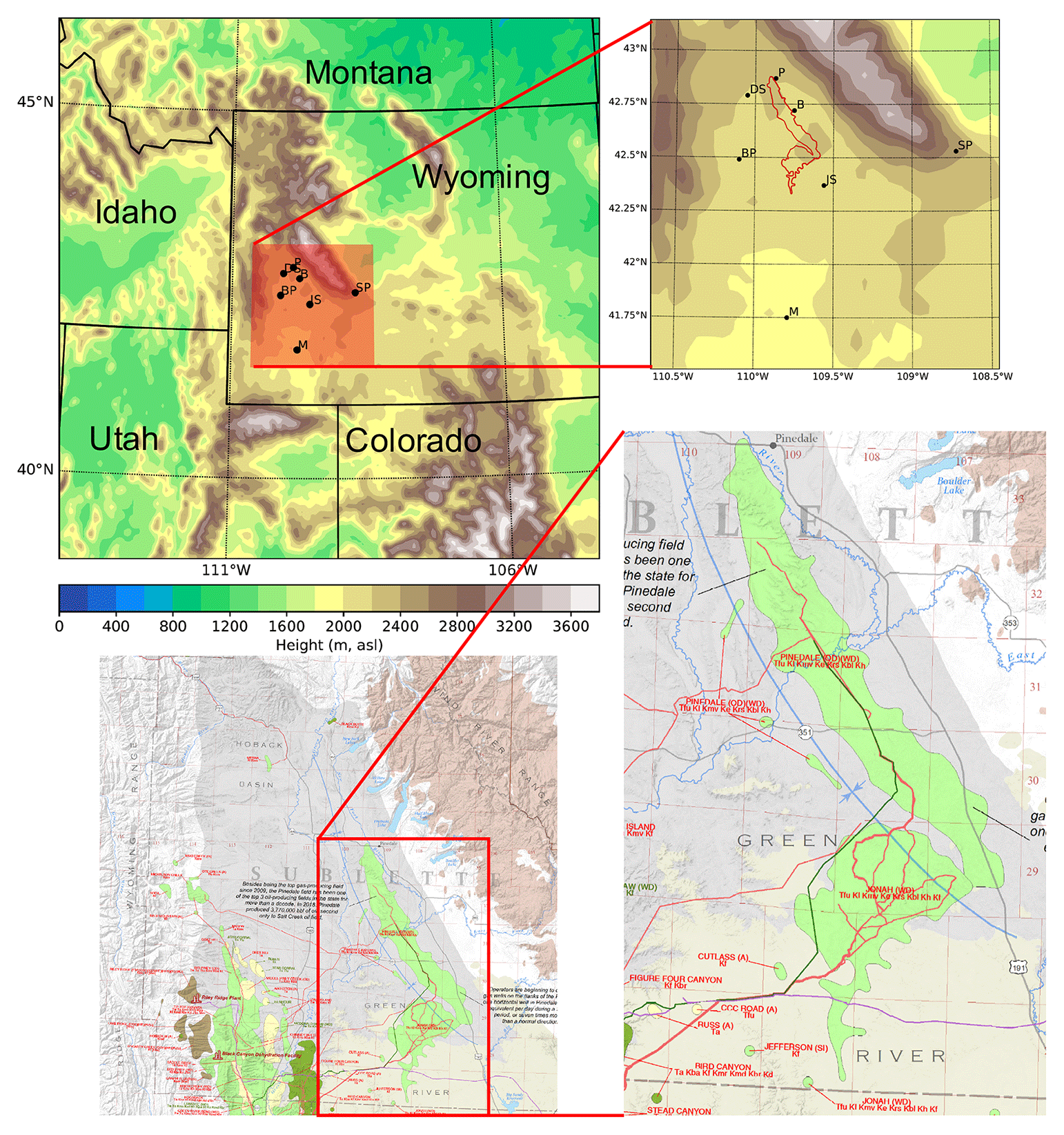
Figure 1 WRF domain (4 km × 4 km grid spacing) with WRF-derived terrain height (upper panels), along with seven weather and air quality monitoring stations in the Upper Green River basin (BP – Big Piney, B – Boulder, DS – Daniel South, JS – Juel Spring, M – Moxa Arch, P – Pinedale, SP – South Pass; shown by the red box). The red outline on the top-right plot is the approximate location of the Pinedale and Jonah Anticline fields derived from the WSGS data depicted in the lower panels. The exact locations of the oil and natural gas wells in UGRB are also shown for reference in the bottom panels. The oil and gas facility data depicted in the lower panels are from Toner et al. (2019), © WSGS.

Table 1 Coordinates and elevations of each weather and monitoring station in the UGRB (source: https://www.wyvisnet.com, last access: 20 February 2021).

2.2 Model setup

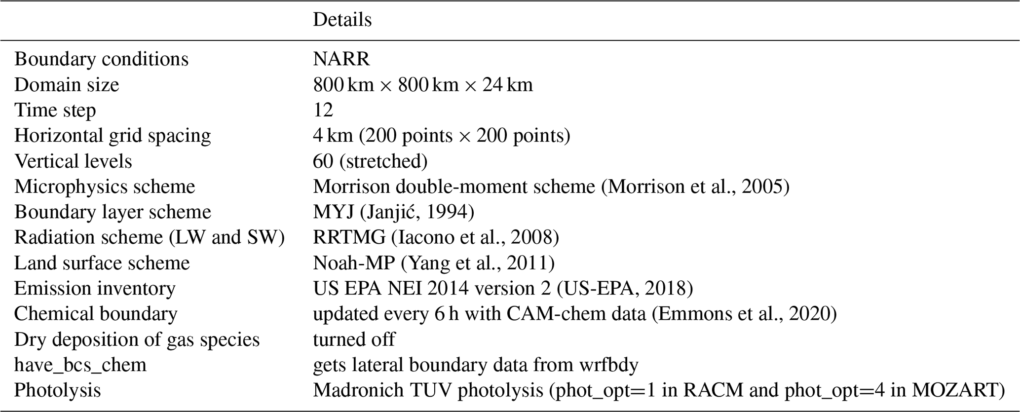
Simulations of O₃ formation in the UGRB were conducted using WRF version 3.9.1 (Skamarock et al., 2008) with Chemistry (Grell et al., 2005). WRF-Chem is a fully coupled model, in which its atmospheric chemistry component is directly coupled to the meteorological component of the model (Grell et al., 2005). The meteorological and air quality components of the model use the same transport and physics schemes as well as the same vertical and horizontal grid structure. This is beneficial over models such as CAMx and CMAQ where the meteorological and the atmospheric chemistry components are simulation separately. Ahmadov et al. (2015) also pointed out a benefit of WRF-Chem in helping in the proper simulation of pollutant accumulation in shallow inversion layers. The model configuration, including the physical and chemical parameterizations used in this study, is shown in Table 2. Figure 1 shows the model domain and terrain height, which is centered on the UGRB. The model domain is represented by a grid of 200 × 200 × 60 points with a horizontal grid spacing of 4 km; vertical grids extend up to 100 hPa, with 60 m grid spacing near the surface and 250 m grid spacing at the top of the model.

(Morrison et al., 2005)(Janjić, 1994)(Iacono et al., 2008)(Yang et al., 2011)(US-EPA, 2018)(Emmons et al., 2020)

Table 2 Model configuration for the base WRF and WRF-Chem simulation. LW and SW denote longwave and shortwave. TUV denotes Tropospheric Ultraviolet and Visible.

2.3 Datasets

The National Centers for Environmental Prediction (NCEP) North American Regional Reanalysis (NARR) (Mesinger et al., 2006) was used for the initial and boundary meteorological conditions for the simulations in this study. The data are available on a Lambert conformal conical grid with a grid spacing of approximately 0.3^∘ (32 km). NARR provides 3-hourly fields on 29 pressure levels from 1000 to 100 hPa.

The emission data for natural gas and oil sources were obtained from the US EPA NEI 2014 dataset (version 2; hereafter, NEI2014v2) released in February 2018 (US-EPA, 2018). The NEI2014v2 data formed the latest emission inventory available at the time of the initiation of this study and are available at a 12 km horizontal grid spacing. This particular version of the emission dataset incorporates the emissions associated with the exploration, drilling, and production of oil, gas, and coal-bed CH₄ wells in the UGRB. The EPA emission estimates widely used and easily available data that include most potential emission sources impacting air quality, although some previous studies (e.g., Alvarez et al., 2018; Robertson et al., 2020) have pointed out underestimations of CH₄ emissions from oil and gas extraction basins in EPA estimates compared to observations. To account for the transport of chemical species into the model domain, 6-hourly data from the Community Atmosphere Model with Chemistry (CAM-chem; Emmons et al., 2020) were used in the simulations.

The observed meteorological and air quality data from the aforementioned seven weather and air quality monitoring stations were obtained from the WYDEQ website. The data are available in 5 min and hourly formats. The hourly data were used for this study for a direct comparison of meteorological parameters, such as temperature and wind speed, and chemical species, such as O₃, NO_x, CH₄, and NMHC, with the simulated results. The NMHC data were only available at the Boulder site as this was the only station equipped to report these results.

2.4 WRF-Chem simulations

The O₃ formation simulations focus on a 4 d period from 3 to 7 March 2017. A spin-up period was not explicitly considered in this study owing to the computational expense of each simulation and because O₃ generally does not start increasing until nearly 24 h into the simulation; however, the results from the first day should still be viewed with caution. For all simulations, the model physics and photolysis surface albedos were modified to account for the effect of snow. The default photolysis albedo in the model is 0.15 because the model was primarily developed for summertime photochemistry. The default photolysis albedo is much lower than what is commonly observed during winter when the surface is covered with snow. Under the default albedo of 0.15, the simulations drastically underestimated O₃ formation (as shown in the results below). Hence, in an effort to simulate a range of potential surface conditions, multiple albedo sensitivity simulations were carried out. A similar study using WRF-Chem with Regional Atmospheric Chemistry Mechanism (RACM) chemistry was carried out by Ahmadov et al. (2015) in the UB, Utah, where they set the surface albedo to 0.85 in their simulations of wintertime O₃ production. However, as noted by Mansfield and Hall (2013), for wintertime O₃ formation, factors such as the thermal inversion and snow cover play an important role and they vary among basins, and thus the findings and characteristics of wintertime O₃ formation cannot be extended from one basin to another. Therefore, in this study, surface albedos of 0.55, 0.65, 0.75, 0.85, and 0.95 were used for the sensitivity study (figure not shown) and fixed to 0.85 in the model for further analysis based on previous estimates of snow albedo in the region (Ahmadov et al., 2015) and sufficient O₃ formation in the UGRB.

In this study, two different chemical mechanisms were used: (i) the Model for Ozone and Related Chemical Tracers (MOZART) and (ii) the Regional Atmospheric Chemistry Mechanism (RACM). The MOZART chemical mechanism has been widely used to study O₃ formation and transport around the world (Hauglustaine et al., 1998; Murazaki and Hess, 2006; Beig and Singh, 2007; Yarragunta et al., 2019). In the UB, RACM has been successfully used to simulate O₃ production due to oil and natural gas production in winter when observed levels of VOCs and NO_x have been used as inputs (Ahmadov et al., 2015). Based on the findings from Ahmadov et al. (2015), the important point noted by Mansfield and Hall (2013), and the MOZART and RACM mechanisms being widely used chemical mechanisms to study O₃ both globally and regionally, the simulations were carried out with these two chemical mechanisms to understand which chemical mechanism provided the best prediction of O₃ compared to observations and its precursors in the UGRB. The WRF-Chem namelist options used for MOZART and RACM are provided in Appendix A, Figs. A1 and A2, respectively. Where possible, the same namelist options were used for both models. However, regarding the photolysis option, the simulations with MOZART used photolysis option 4, which is the updated TUV photolysis option based on recent advances in the understanding of photolysis rates that was configured to work with only a few chemical-mechanism schemes in WRF-Chem v3.9.1, while the RACM simulations used photolysis option 1, which is the Madronich photolysis scheme.

2.5 Preprocessing

The EPA anthro_emiss tool provided by the Atmospheric Chemistry Observations & Modeling (https://www2.acom.ucar.edu/wrf-chem/wrf-chem-tools-community, last access: 11 October 2019) (ACOM) division at the National Center for Atmospheric Research (NCAR) was used for preprocessing the emissions in this study. This tool creates anthropogenic emission files from the NEI datasets that can be ingested into the WRF-Chem model. Because the MOZART and RACM chemical mechanisms use different species groupings, the emission inventory files were processed separately for each mechanism. Additionally, mozbc, which is also provided by ACOM, was used in this study to map the chemical species from the CAM-chem global dataset to WRF-Chem fields initial and boundary condition files.

For simulations using the MOZART chemical mechanism, two other WRF-Chem utilities were also used: exo_coldens and wesely. The exo_coldens utility reads O₃ and O₂ climatological atmospheric column data rather than using fixed values, and this is coupled to the aforementioned updated TUV photolysis option (phot_opt=4). For dry deposition in MOZART, the wesely utility is used to account for seasonal changes in dry deposition. Both the exo_coldens and wesely utilities read the WRF-Chem input files and emission files to produce additional data files for WRF-Chem simulations conducted with the MOZART chemical mechanism.

2.6 Model validation

To study the ability of the model to replicate observed meteorological conditions in the UGRB, we study the temperature inversion, weak winds, and surface temperature. Owing to differences in data availability (e.g., observations and emission inventories), two different periods are selected for meteorology validation. Specifically, the temperature inversion was studied using the WRF model (without chemistry) for 2011, while the surface meteorology was validated using the focus period in March 2017, and the details of these analyses are provided below. Additionally, wintertime O₃ was measured in the UGRB from February to March 2017 by WYDEQ, providing an additional dataset to validate the WRF-Chem model, albeit with a strict focus on O₃ precursors.

2.6.1 Temperature inversion validation

Owing to the aforementioned data availability limitations, in addition to the WRF-Chem simulations focused on the high-O₃ event in March 2017, additional simulations using WRF but without chemistry were conducted for the entire winter of 2011 (1 December 2010 to 31 March 2011, hereafter referred to as IOP11, in which “IOP” stands for “intensive operation period” and “11” refers to the year of simulation), encompassing the period during which vertical profiles of temperature and O₃ from ozonesondes were collected by the WYDEQ Air Quality Division (AQD) in winter 2011 (MSI, 2011; 28 February to 2 March and 9 to 12 March). The IOP events were identified based on the conditions (deep snow with large spatial coverage in the study area, development of an inversion, and calm surface winds) that support elevated O₃ mixing ratios. During each IOP, three to four ozonesondes were launched adjacent to the Boulder station (see Fig. 1) each day, providing vertical profiles of O₃ mixing ratio, temperature, and wind speed. We note that the data from year 2011 were utilized because this is the only year for which vertically resolved meteorological data were available from radiosondes. Further, we understand that the ability of the model to simulate one event (i.e., the vertical structure for a few days in 2011) does not indicate that it will perform accurately again. However, given that basin-wide emission estimates from WYDEQ have decreased significantly over the last decade with potential impacts on both O₃ precursor mixing ratios and VOC : NO_x ratios, as well as the unavailability of emissions for oil and gas from 2011, the IOP11 simulation is only used herein to validate simulated temperature inversions, and the focus of the remainder of this work is on the high-O₃ events that occurred in March 2017.

2.6.2 Surface meteorology validation

The surface meteorology in the WRF-Chem simulations detailed in Sect. 2.4 was validated against observations collected at seven monitoring stations (Big Piney, Boulder, Daniel South, Juel Spring, Moxa Arch, Pinedale, and South Pass) by WYDEQ, with a focus on temperature and wind speed, two factors that greatly impact the accumulation of O₃, as described in Sect. 1. While wind direction is another important variable for pollutant transport, given the low wind speeds that occur during high-O₃ events, the model's ability to precisely simulate the observed wind directions is of less importance to this study. Moreover, such a comparison could be greatly affected by sampling issues owing to the high variability in observed and simulated wind directions under nearly calm conditions.

2.7 VOC and NO_x sensitivity study

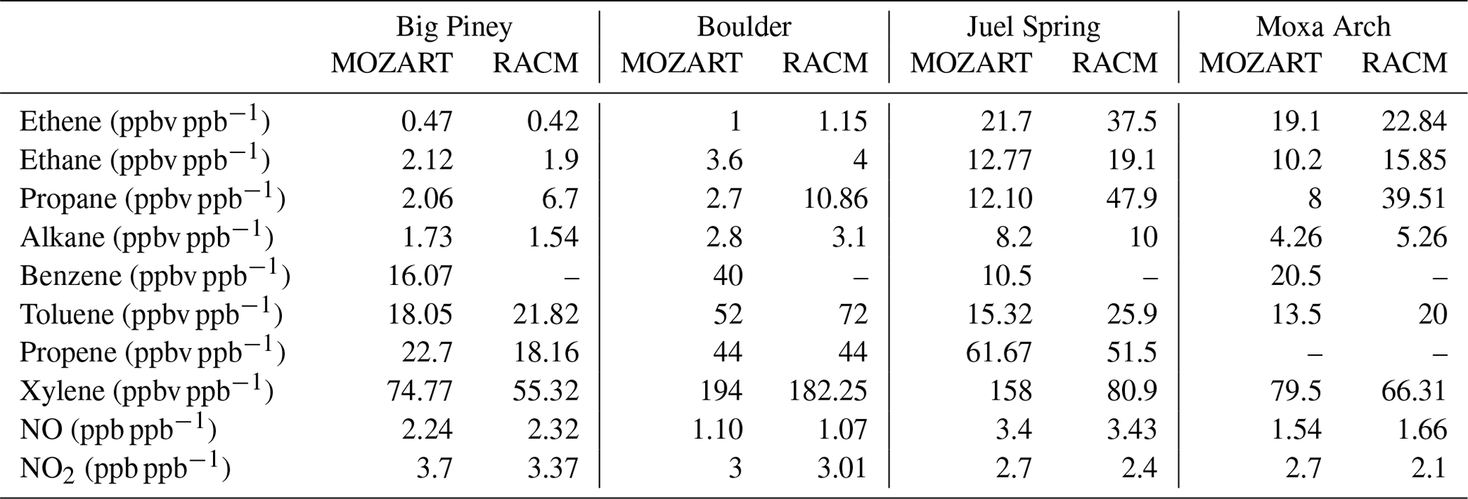
WYDEQ carried out a wintertime O₃ study from February to March 2017, coinciding with the high-O₃ event that is the focus of this study. On several days during this period, speciated VOC canister measurements were collected between 04:00 and 07:00 MST at Boulder, Big Piney, Juel Spring, and Moxa Arch (MSI, 2017). The speciated VOC data from all stations on 3 March 2017 were compared with the respective WRF-Chem model data. Table B1 in Appendix B shows ratios of canister-observed speciated VOC mixing ratios to the simulated values. The Moxa Arch site is relatively far from the emission sources and is not representative of the main O₃ formation region. The other sites show variability, although all sites show significant underestimates of both VOCs and NO_x. The Boulder site has the largest underestimates of reactive benzene, toluene, ethylbenzene, and xylene (BTEX) species, while some species have larger underestimates at other sites. Given this comparison and the site-to-site variability in the model–observation comparison, VOCs measured at the Boulder site appear to be a reasonable, though aggressive, basis for adjusting the emissions in the model. For NO_x, because the data are available for the entire study period, factors for NO and NO₂ were calculated taking into account the entire study period (3 to 7 March 2017; see Fig. B1 in Appendix B for details on the time series), as shown in Table 5.

Using the above model–observation comparison, four additional simulations using each chemical mechanism were carried out to study the sensitivity to NO_x and VOC emissions. The precursors' emissions were adjusted in each simulation based on the factors shown in Table 5. The emission adjustment factors for VOCs in Table 5 were calculated by dividing the observed values (canister) by the model-simulated values for the same time period. The goal of this analysis and additional sensitivity simulations was to (1) adjust NO and NO₂ to better match the observations and (2) test the sensitivity of O₃ production to NO_x levels. In all, four additional sensitivity simulations were conducted using the aforementioned emission adjustment factors for VOCs and NO_x: (1) increased VOCs only, (2) increased NO_x only, (3) increased VOCs and NO_x, and (4) increased VOCs and doubled NO_x (here, “doubled” indicates that the emission adjustment factor was doubled).

The adjustments for certain VOC species that are lumped in the model chemistry require slightly more explanation. For alkanes, the mixing ratios of all observed alkane species larger than propane (butane up to undecane) were summed, and then this sum was used to adjust the lumped model species (BIGALK for MOZART and HC5 for RACM). In RACM, the species TOL is a combination of toluene and a fraction (0.293) of benzene. Accordingly, a fraction of the observed benzene was added to the observed toluene to adjust this variable. Also, in RACM, the species HC3 is a combination of methanol, ethanol, and a fraction (0.519) of propane. The WYDEQ observations do not include methanol or ethanol, meaning only the observed propane mixing ratio was used to modify this variable. Finally, in both models the lumped xylene parameter includes trimethylbenzene. Accordingly, the observed mixing ratios of xylene and trimethylbenzenes were grouped to calculate the emission adjustment factor for xylene.

3 Results and discussion

We first validate the WRF model's performance in simulating the observed vertical temperature profile and surface meteorology during strong inversions (see Sect. 2.6.1 for details). After determining that WRF is able to reasonably reproduce the meteorological conditions necessary for O₃ formation, we analyze O₃ formation with WRF-Chem using two different chemical mechanisms and multiple sensitivity simulations.

3.1 Validation of WRF model meteorology

3.1.1 Temperature inversion

Owing to the importance of thermal inversions for the buildup of O₃ in wintertime events, we first explore the ability of the model to simulate temperature inversions within the selected modeling framework. Vertical profiles of the observed temperature and O₃ mixing ratio during the most recent IOPs (28 February to 2 March and 9 to 12 March 2011) are compared with the simulated vertical temperature profiles from WRF simulations during the same time period (IOP11, Fig. 2). Although 7 d is identified as the IOP, the results from only 4 d are discussed due to ozonesonde data availability. Because these simulations are performed to compare meteorology and not chemistry, the WRF model without chemistry is used, and simulated O₃ is not available. We do not aim to simulate O₃ events from 2011 because emissions have changed dramatically since 2011 and there is no good inventory that includes oil and gas sources for that period. Observed O₃ is presented only to demonstrate how O₃ formation follows the inversion events.

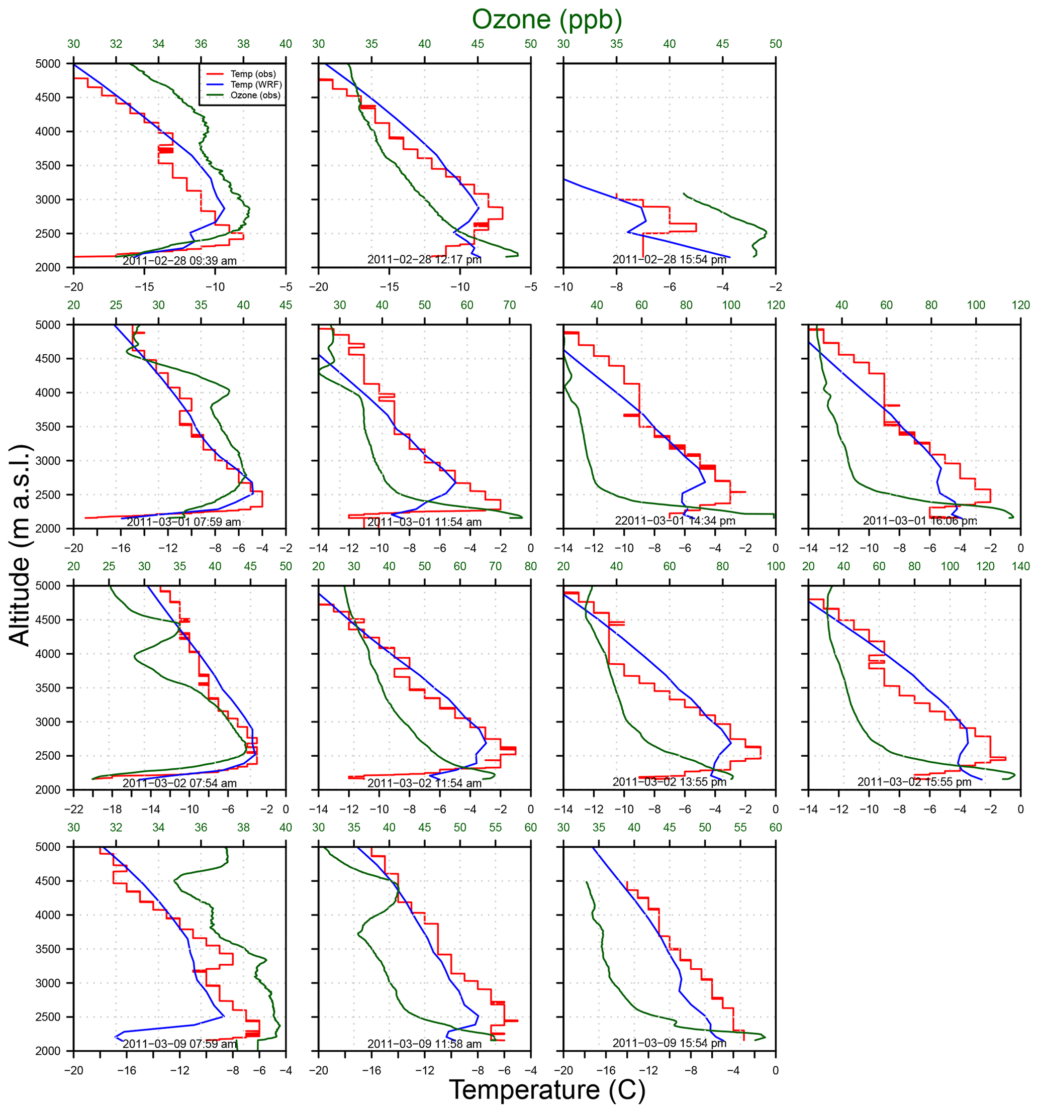
Figure 2 Vertical profiles of O₃ (ppb, green) and temperature (^∘ C, red) from ozonesondes launched in 2011 by WYDEQ compared to WRF-simulated temperature (^∘C, blue) for 4 d. Each row represents three to four ozonesondes launched in 1 d.

A shallow mixing height can be seen in each profile. The residual layer above the ground appears to be well mixed early in the simulation; hence, we can see fairly uniform O₃ mixing ratios in the observed profiles. High mixing ratios of O₃ are observed on 1–2 March 2011. On these days, a strong inversion is observed with a shallow mixing height of around 500 m a.g.l., which prevents vertical mixing, thus leading to a buildup of O₃ precursors and high mixing ratios of O₃ that increase in the afternoon (MSI, 2011). On 2 March 2011 (Fig. 2, third row), higher morning O₃ is observed compared to the previous day, presumably due to the persistent inversion, which is validated by the observation of high hydrocarbon mixing ratios in the afternoon of 2 March (MSI, 2011).

For the days discussed here, the simulated temperature is 2 to 4 ^∘C warmer than the observed temperature, except for 9 March 2011 (Fig. 2, last row), where it is 2 to 5 ^∘C colder than the observed temperature near the surface. During the morning hours, the simulated temperatures follow the observed temperatures fairly well; however, the simulated inversion height is slightly elevated. In both the observations and the model, the inversion height increases through the day and the inversion strength (difference in maximum vs. surface temperature) decreases. However, the model seems to increase the inversion height slightly too much while also decreasing the strength of the inversion. Overall, the model simulation of the inversion events is deemed adequate to proceed.

3.1.2 Surface meteorology

Given the model's ability to reasonably represent temperature inversions, at least based on our comparison with available data from 2011, we further assess the model's ability to predict surface meteorology focusing on the target period of high O₃ in March 2017. It is important to highlight again that vertical data are not available for the selected time period. We utilize observations from the high-O₃ events of 2017 because the seven ground stations measure basic meteorological parameters. It is crucial for the photochemical model to simulate low temperatures and calm winds to be able to replicate high O₃ mixing ratios (Schnell et al., 2009).

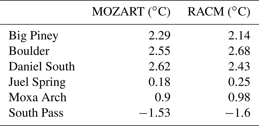
The observed 2 m temperature data for Pinedale are unavailable; hence the temperature correlations for only six stations are shown in Fig. 3. Simulations with both chemical mechanisms show good correlation with the observed temperatures, and the correlation coefficients do not show any sensitivity to the different chemical mechanisms at the Juel Spring and Moxa Arch stations. However, RACM shows higher correlation coefficients compared to MOZART at other stations (except Boulder). The difference in the correlation coefficients for the different chemical mechanisms is small and likely due to radiation feedbacks between the chemistry and meteorology as well as internal model variability (Bassett et al., 2020). Furthermore, the temperature bias between the observed and simulated datasets is below 3 ^∘C at all stations (Table 3), and all of the data points lie in close proximity to the 1:1 lines. Overall, the simulations show good correlation with the observed 2 m temperatures.

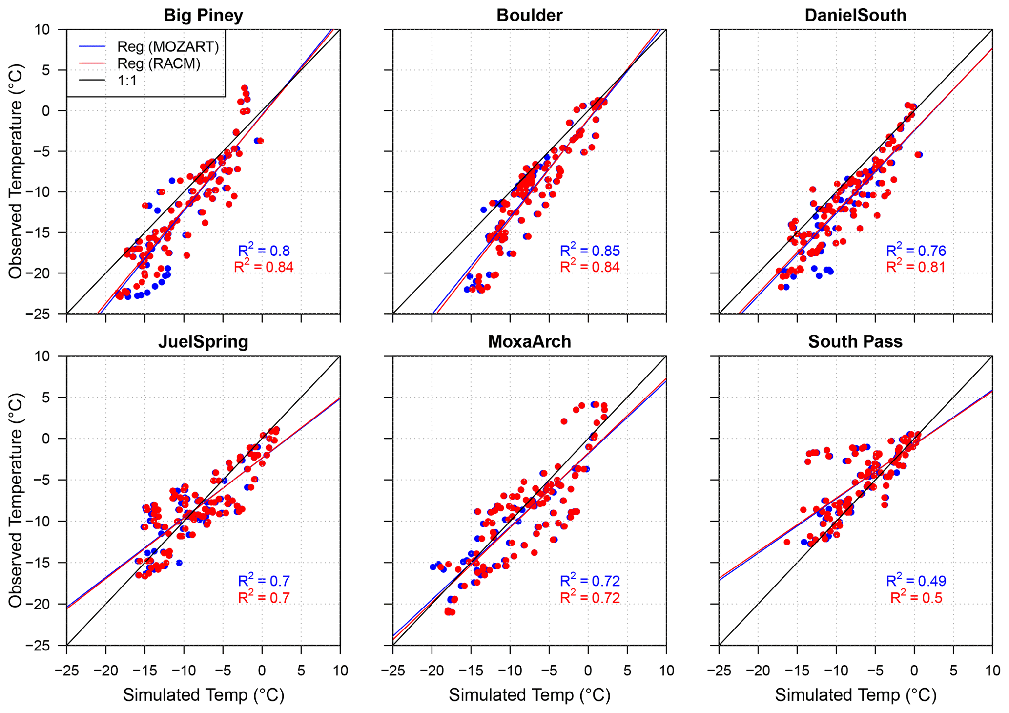
Figure 3 Correlation between observed and simulated 2 m temperature at six monitoring stations. The data points and regression line for MOZART and RACM are shown in blue and red, respectively. The 1:1 lines are represented by black lines in each plot.

Table 3 Temperature bias (in ^∘C) for the MOZART and RACM simulations.

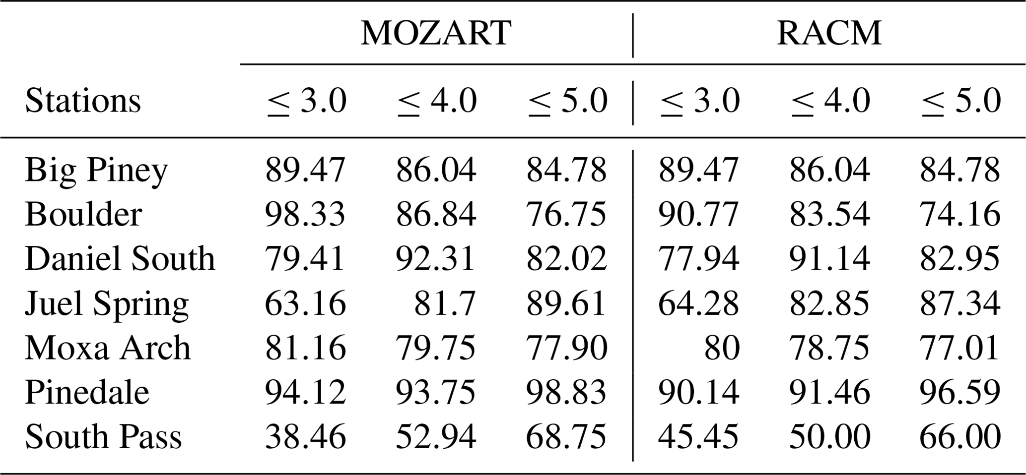
As mentioned earlier, calm winds are an essential meteorological condition for the photochemical production of wintertime O₃ because they are necessary for the accumulation of O₃ precursors. The correlation between observed and simulated wind speeds is shown in Fig. 4. The correlation coefficients are calculated for each data point (hourly) for the entire study period, although only wind speeds from 0 to 10 m s⁻¹ are shown given the focus of the study on calm periods with high O₃ mixing ratios. For all stations except South Pass, a majority of the data points are clustered below or around 4 m s⁻¹ in both the observations and the model simulations. The differences in the correlation coefficients between different simulations are due to internal model variability (Bassett et al., 2020). Furthermore, the relatively low correlation coefficients may be the result of small variations in low wind speeds. To test this notion and to verify that calm periods are successfully simulated, Table 4 shows the percentage of time that the simulated and observed wind speeds are less than or equal to different thresholds (3, 4, and 5 m s⁻¹). For example, at Boulder, both the simulated wind speeds using MOZART and the observed wind speeds are less than or equal to 3 m s⁻¹ for 98.33 % of the analysis period, while for RACM this figure is 90.77 %. Again, the chosen thresholds are based on the interest in studying calm wind speeds in the basin, which limit pollutant transport/dispersion and enable pollutant accumulation near the surface. Therefore, even though the correlation coefficients between the modeled and observed winds are relatively low, we conclude from the results in Table 4 that WRF with either chemical mechanism is able to successfully predict low wind speeds for most of the study period. An analysis of the diurnal variability in winds also shows reasonable qualitative agreement between the model and observations in terms of the timing of increasing and decreasing wind speeds each day, especially on days with elevated O₃ mixing ratios (figure not shown).

Figure 4 Similar to Fig. 3 but for wind speed.

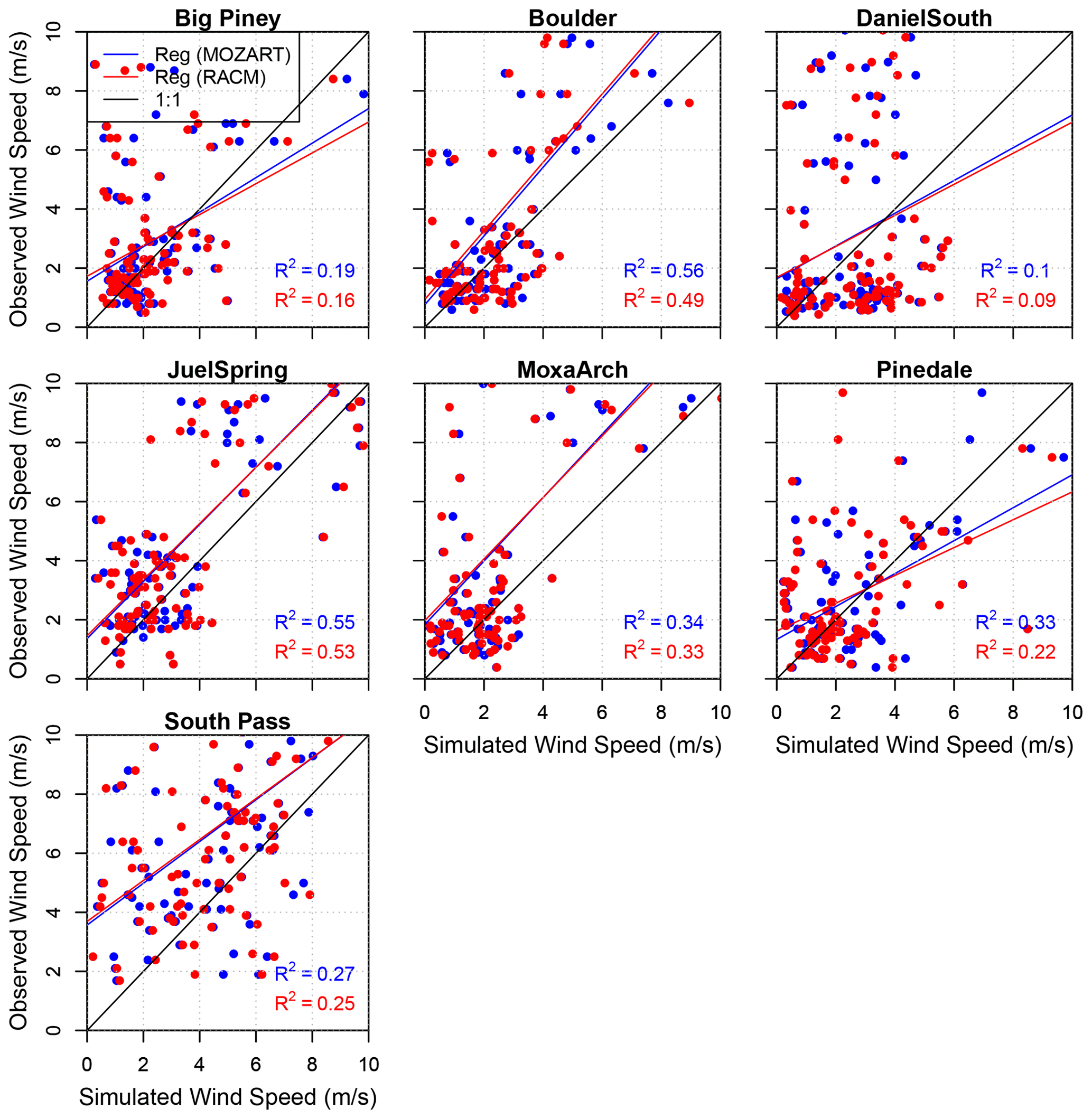
Table 4 Percentage of the data points that are less than or equal to the given threshold (in m s⁻¹) when the observed wind speed is also less than or equal to the same threshold.

3.2 Baseline simulation and O₃ production

Given the aforementioned ability of the model to adequately simulate the key meteorological conditions needed for O₃ production and accumulation, we now turn to an analysis of the chemical mechanisms and their ability to reproduce the observed hourly periods of high O₃. At first, O₃ formation was simulated in the UGRB using RACM, and it was noted that the modeled mixing ratios were dramatically below the observed O₃ levels. However, the default WRF-Chem model has a low photolysis albedo (0.15) as it was intended to simulate summertime O₃. We modified the photolysis albedo in the model based on more typically wintertime conditions following Ahmadov et al. (2015), who noted that in the UB, it was necessary to increase the photolysis albedo to accurately simulate O₃ production. Further, in this study, additional simulations were conducted to analyze the sensitivity of O₃ formation to the photolysis albedo in the WRF-Chem model, spanning albedos representative of partially snow-covered vegetation to fresh, deep snow, and compared the results with those obtained using the default albedo of 0.15. All of the albedo sensitivity tests used RACM. Figure 5 compares the default albedo (0.15) with different photolysis albedo settings (0.65 and 0.85). It is evident that the default photolysis albedo produces much lower O₃ mixing ratios at all stations. However, when the model is altered to use an albedo of 0.85, the diurnal variation and high O₃ peaks are captured relatively well, although there is some variability from station to station. For the remainder of the simulations in this paper, a photolysis albedo of 0.85 is used, which is the same albedo used by Ahmadov et al. (2015) in the UB.

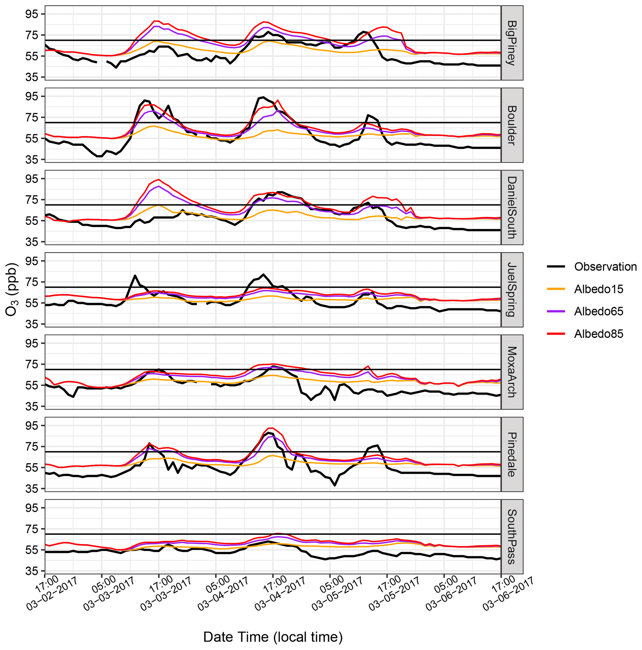
Figure 5 Albedo sensitivity for the WRF-Chem simulation at seven monitoring stations. The observed O₃ mixing ratios at each station are shown in black lines; the orange lines represent the results from the default photolysis albedo of 0.15; and the purple and red lines are the modified photolysis albedos of 0.65 and 0.85, respectively. The NAAQS 2015 standard is shown by the black lines on each plot. The date format here and in subsequent figures is month-day-year.

Setting a fixed photolysis albedo of 0.85, we next compared simulations using two different chemical mechanisms available in WRF-Chem: MOZART and RACM. Figure 6 compares the time series of simulated hourly O₃ mixing ratios from four different simulations with dry deposition of gas species included and not included in both MOZART and RACM simulations at several UGRB monitoring stations. The hourly averaged observed background daily O₃ mixing ratio is approximately 55 ppb at all stations. During the afternoon hours, most of the stations have hourly O₃ mixing ratios greater than 70 ppb. The observed O₃ mixing ratios are highest at the Boulder site, which is likely because it lies in close proximity to the PAJF production facilities and is thus closer to the main sources of VOC precursors than the other sites. For Moxa Arch and South Pass, the observed O₃ mixing ratios are lower because they do not lie in close proximity to the wells and also lie further from the basin.

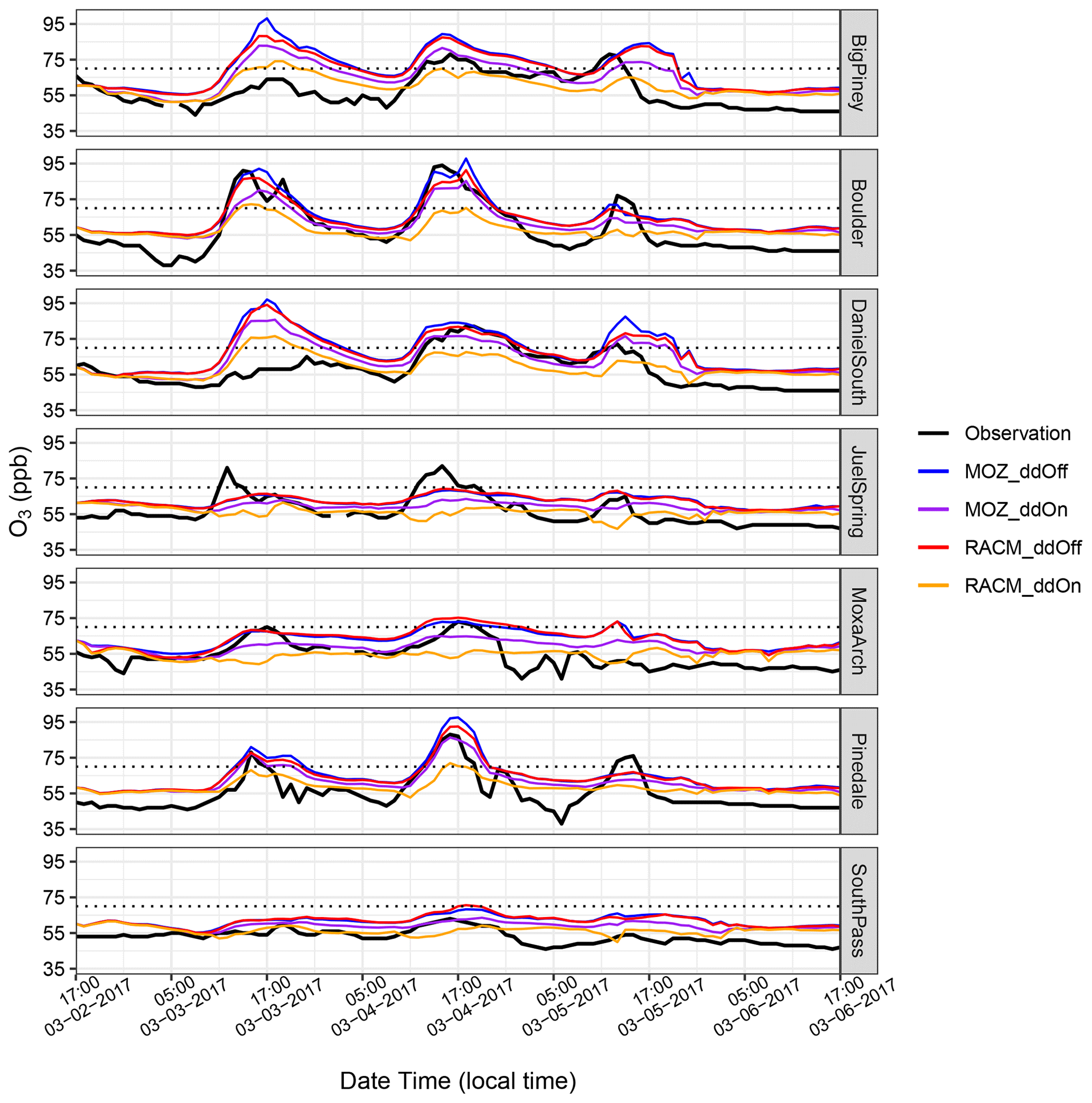
Figure 6 Time series of O₃ mixing ratios at seven monitoring stations for the time period of 3 to 7 March 2017, along with the 8 h National Ambient Air Quality Standard 2015 (dotted black lines). MOZART simulation with dry deposition of gas species not included is represented by blue lines, and the RACM simulation without the dry deposition is represented by red lines. The MOZART and RACM simulations with the inclusion of dry deposition of gaseous species are represented by purple and orange lines, respectively.

To better understand the chemical mechanisms' sensitivity to dry deposition, we also compare the diurnal variation in O₃ mixing ratios from MOZART and RACM with dry deposition turned off at the seven monitoring stations. The justification for these additional simulations is that simulations using RACM with dry deposition of gas-phase species do not produce sufficient O₃ compared to observations (Fig. 6, orange lines). In MOZART, when dry deposition is turned on, it adjusts the deposition rate over snow surfaces (owing to the use of the wesely preprocessing tool that adjusts the seasonal change in dry deposition), where the loss is expected to be greatly reduced. RACM does not adjust the dry deposition rate over snow-covered surfaces; hence the dry deposition is likely too high in RACM and could explain the underestimate of O₃. Thus, we turned off dry deposition to mimic the very slow deposition of gas-phase species over snow-covered surfaces (i.e., RACM_ddOff). Despite these large differences in the results from the simulations when the dry deposition of gas species is included, when dry deposition is turned off, both MOZART (MOZ_ddOff; Fig. 6, blue lines) and RACM (RACM_ddOff; Fig. 6, red lines) produce similar mixing ratios of O₃, suggesting that a large reason for the disparity in results under the different chemical mechanisms is related to the formulation of dry deposition of gas species.

Shifting focus to the individual sites, at Big Piney and Daniel South, which are located on the eastern side of the Wyoming Range, all four simulations overestimate the first O₃ event (3 March 2017 at 15:00 local time). However, as noted earlier, the model results from the first day should be viewed with caution. Moreover, the MOZ_ddOff and RACM_ddOff simulations capture the diurnal cycle of O₃ reasonably well at Boulder, while they overestimate the high-O₃ event at Pinedale on 3 March 2017, 17:00 LT, which is well captured by MOZ_ddOn. However, the simulations miss the higher O₃ mixing ratios at Juel Spring. Overall, both the MOZ_ddOff and the RACM_ddOff simulations do reasonably well at simulating the O₃ mixing ratios in the UGRB for the selected study period and capturing the diurnal variation in O₃, a first for a photochemical model using an existing emission inventory, although it is important to remember that this was only possible after adjusting the photolysis albedo in the model and, in the case of RACM, turning off dry deposition of gas-phase species. Due to their better performance in estimating observed O₃, the results from MOZ_ddOff and RACM_ddOff simulations will be discussed in the following analyses, and the simulations will be referred to as MOZ17 and RACM17, respectively.

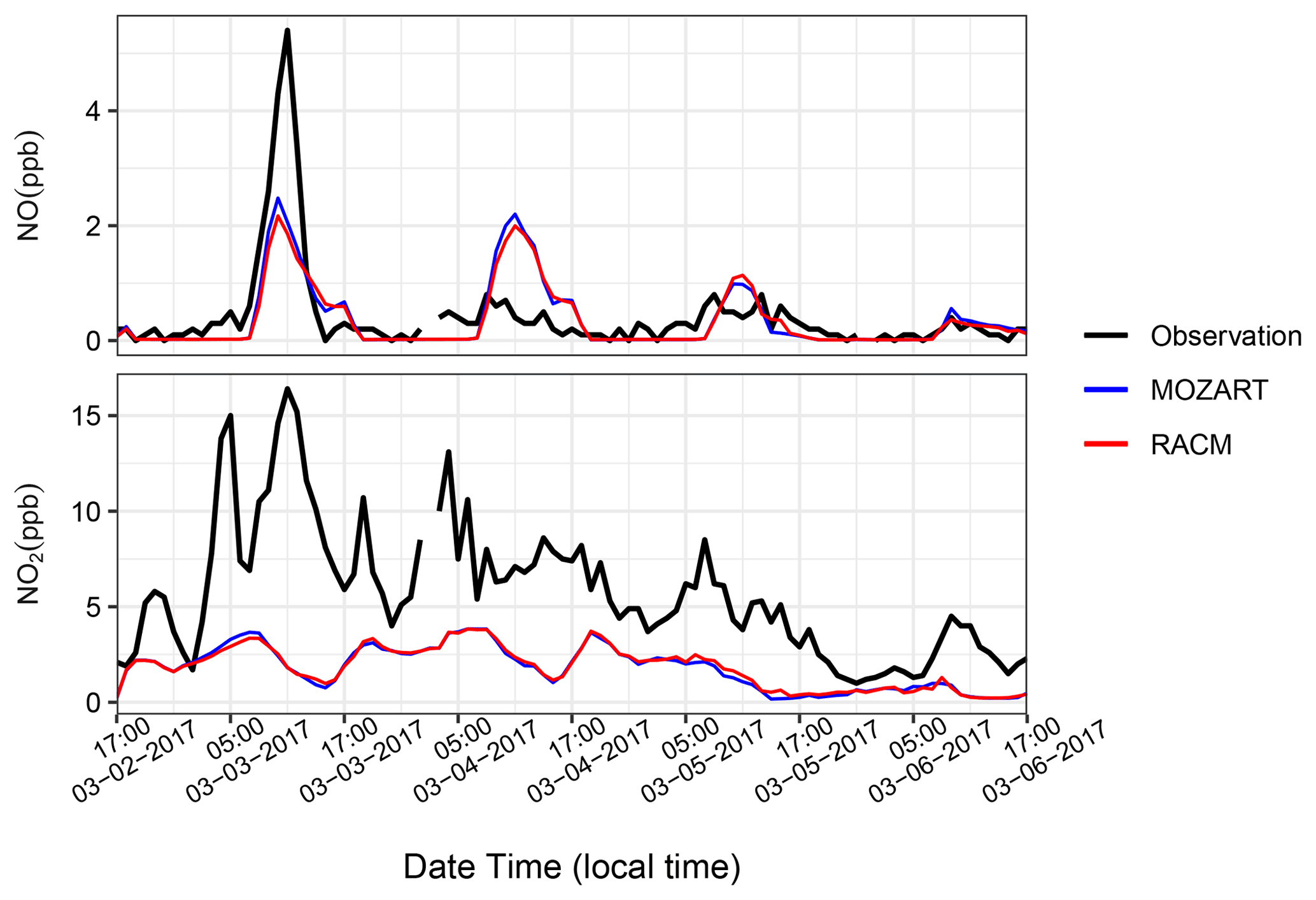
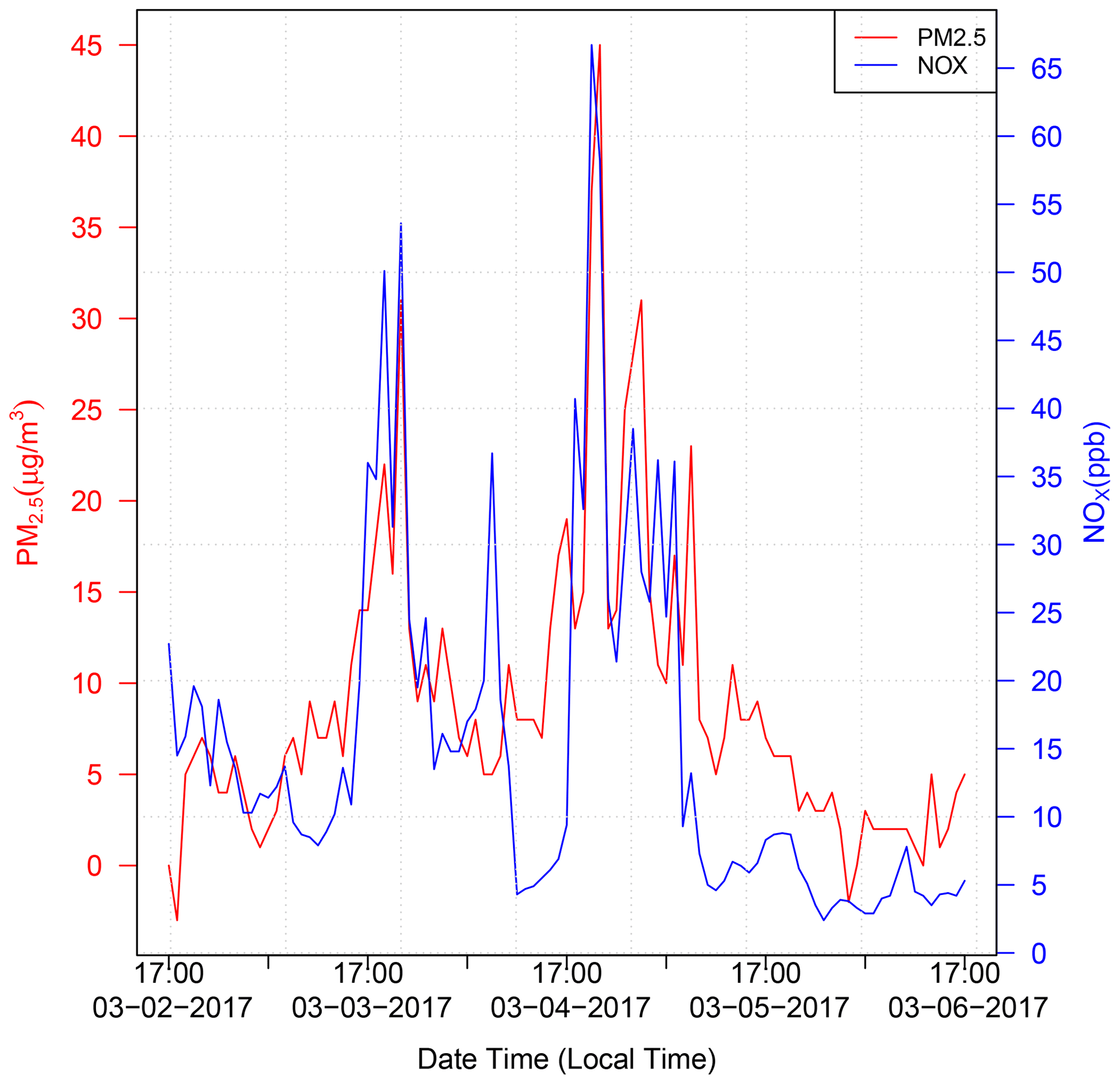
To better understand the differences in the simulated and observed O₃ mixing ratios, we next looked at the precursor mixing ratios. Figure 7 shows the time series of hourly NO_x at the seven monitoring stations, along with results from MOZ17 and RACM17. The observed hourly mixing ratios of NO_x at Big Piney, Boulder, and Pinedale are higher than at the other stations. These three stations are all near small towns in the region, with Pinedale being the largest of the towns and having notably higher NO_x than the others. Moreover, in Pinedale, there are sources of NO_x that are not related to oil and gas, most notably residential wood burning. However, residential wood burning is not well represented in the emission inventory; thus, the model is expected to underestimate NO_x in such areas. The elevated observed NO_x mixing ratios compare well with the observed PM_2.5 at Pinedale (Fig. C1 in Appendix C), which supports the conclusion that wood burning is a strong NO_x source in this area. The simulated mixing ratios of NO_x are less sensitive to the different chemical mechanisms, emphasizing that the emissions dominate the mixing ratios and not chemical loss mechanisms. The NO_x mixing ratios are underestimated by both simulations even during the high-O₃ events. Although the simulated NO_x mixing ratios at Daniel South are higher compared to the other stations, the observed data are missing. The observed and simulated NO_x mixing ratios at South Pass are low and show little variability, as expected given that this station is further from the oil and gas production region. Overall, the simulations underestimate the observed NO_x mixing ratios to varying degrees depending on the location and do not capture the diurnal cycle well, which poses a conundrum given the reasonably good agreement between simulated and observed O₃ mixing ratios.

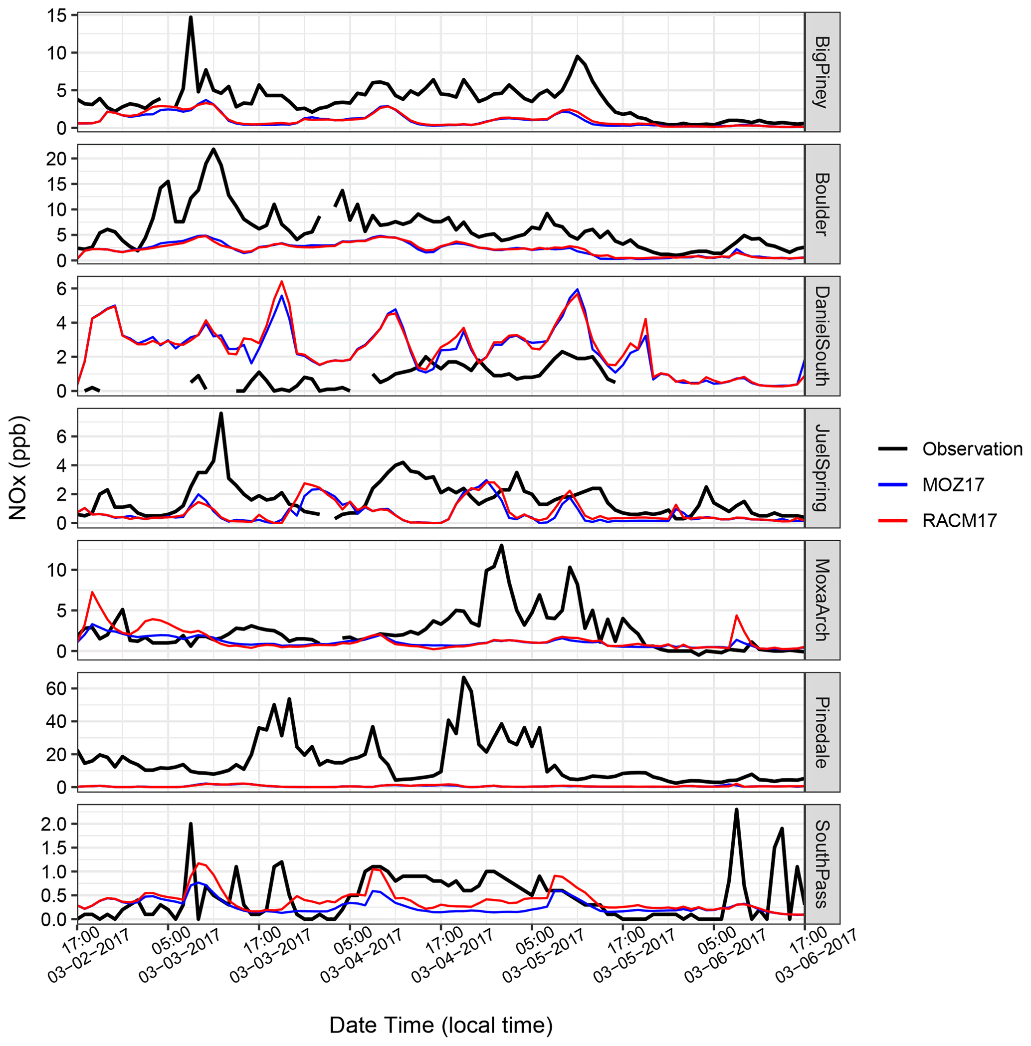
Figure 7 Similar to Fig. 6 but for NO_x mixing ratios (note the different y scales for each station).

In the top panel of Fig. 8, we next compare the simulated NMHC mixing ratios (plotted on the left, primary y axis) and observed NMHC mixing ratios at the Boulder station (plotted on the secondary y axis). The Boulder station is the only monitoring site in the basin that measures either NMHC or CH₄. In addition, the MOZART² and RACM³ chemical mechanisms lump the VOC species differently. The bottom panel of Fig. 8 shows the observed O₃ mixing ratios at the Boulder station during the same time period, showing that the accumulation of NMHC leads to the production of O₃. Although the temporal evolution of NMHC is well captured by the simulations, the magnitudes of the simulated NMHC mixing ratios are lower by a factor of approximately 6 compared with the observation. Both RACM17 and MOZ17 give very similar NMHC mixing ratios because the chemical production of O₃ does not remove a large amount of the NMHC present. When it was discovered that the model-simulated VOC mixing ratios were substantially lower than the observations at the Boulder site, we employed University of Wyoming mobile laboratory data to confirm that the Boulder site does not record anomalously high mixing ratios relative to the surrounding area as the station sits in a small valley. The mobile lab did not measure NMHC, but both the mobile lab and the Boulder station measured CH₄ enhancements, which are a reasonable proxy for VOC enhancements, thus enabling us to see if CH₄ measurements made by the lab in the region surrounding the Boulder site were significantly different than those reported by the site. We compared the CH₄ mixing ratios collected by the mobile lab during an O₃ event in 2020, the closest year to our study period for which data are available. The WYDEQ Boulder data were within 25 % of the data collected by the mobile lab near the monitoring site (Fig. D1 in Appendix D). This observation indicates that the difference between the simulated and observed NMHC mixing ratios is not the result of anomalously high mixing ratios at the Boulder site, and thus the NMHC mixing ratio measured at the Boulder site is an accurate representation in the region.

Figure 8 Time series of NMHC (a) and O₃ (b) at the Boulder site.

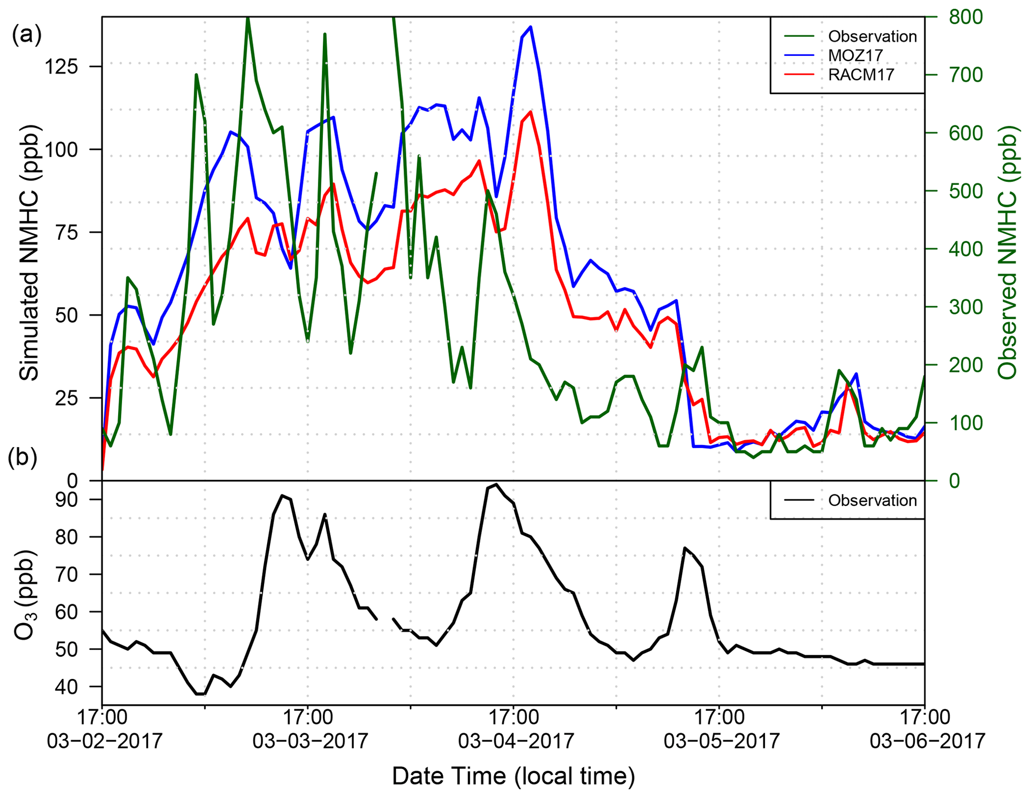
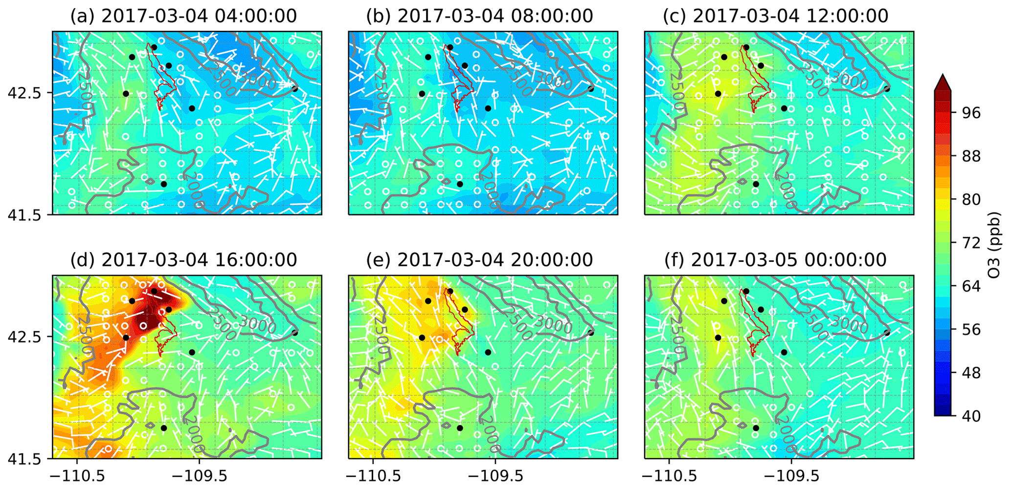
Figure 9 Formation and dissipation of O₃ over the basin using MOZART chemistry with dry deposition of gas species turned off (MOZ_ddOff) for the O₃ event on 4 March 2017, starting at 04:00 and ending at 24:00, with an interval of 4 h in two consecutive panels. All times in the figure are in local time (UTC−7). The black dots are the location of the seven WYDEQ stations, and the red outline is an approximate location of the PAJF development.

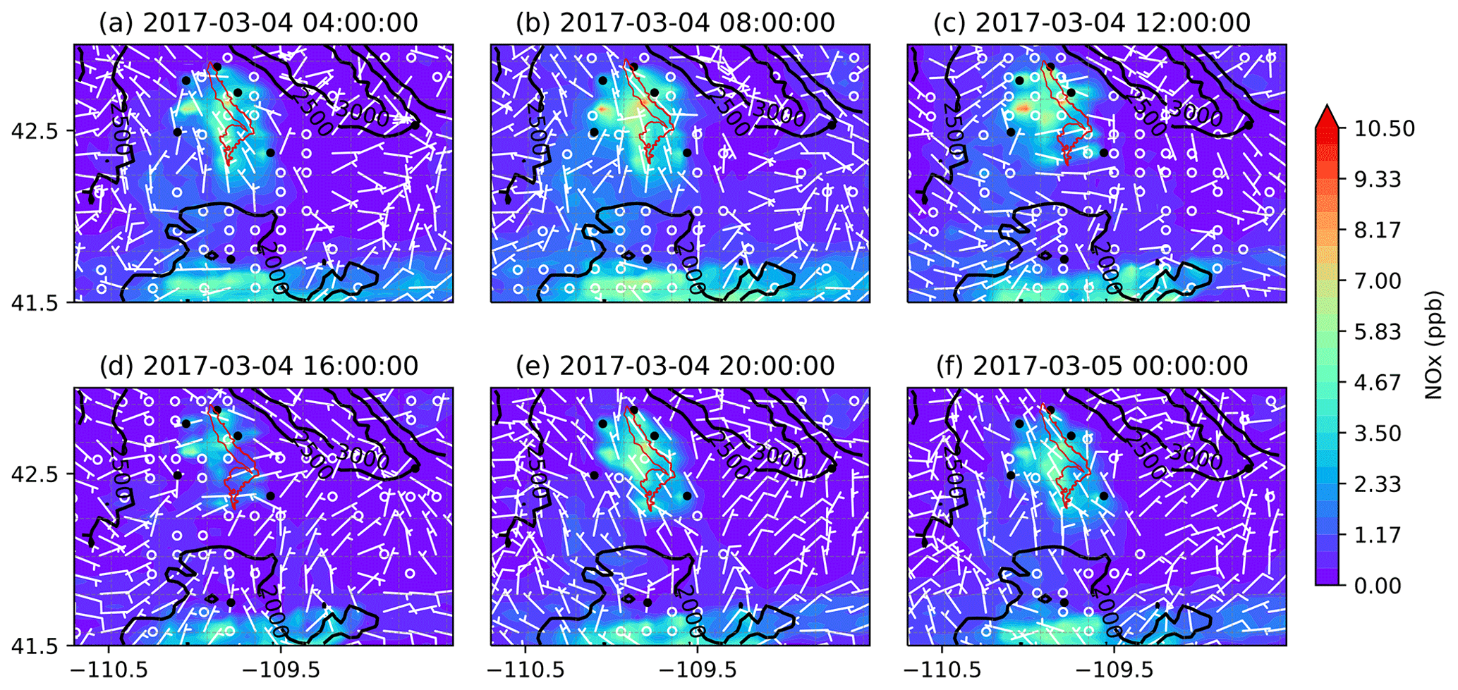
Figure 10 Similar to Fig. 9 but for NO_x mixing ratios.

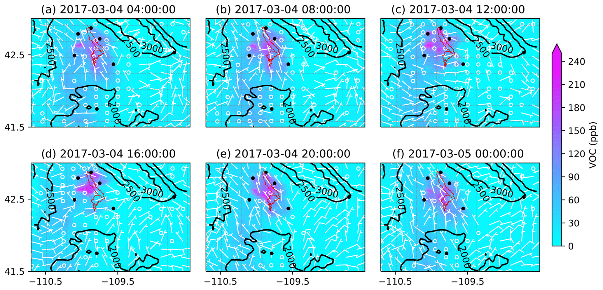
Figure 11 Similar to Fig. 9 but for the mixing ratios of VOCs.

It is very intriguing that both chemical mechanisms are able to reasonably replicate the O₃ mixing ratios at the monitoring sites despite the fact that NMHC mixing ratios in the model are approximately 6 times lower than those observed at the Boulder monitoring site, and NO_x is also generally underestimated. The mobile lab results strongly suggest that this discrepancy is not due to non-representative measurements at the Boulder monitoring site. This leaves the possibilities that the simulated NMHC compounds are much more reactive than the actual NMHCs, that some other feature of the chemistry is too active in the model, and/or that the UGRB will continue to experience high-O₃ events even at much lower NMHC levels because O₃ production is predominantly determined by NO_x availability. In terms of the possibility that the chemistry in the model is too active, it is important to note that the RACM17 chemistry successfully simulated O₃ events in the UB when observed NO_x and speciated VOCs were input (Ahmadov et al., 2015). The sensitivity to adjustments in speciated VOC and NO_x emissions is discussed later in Sect. 4.

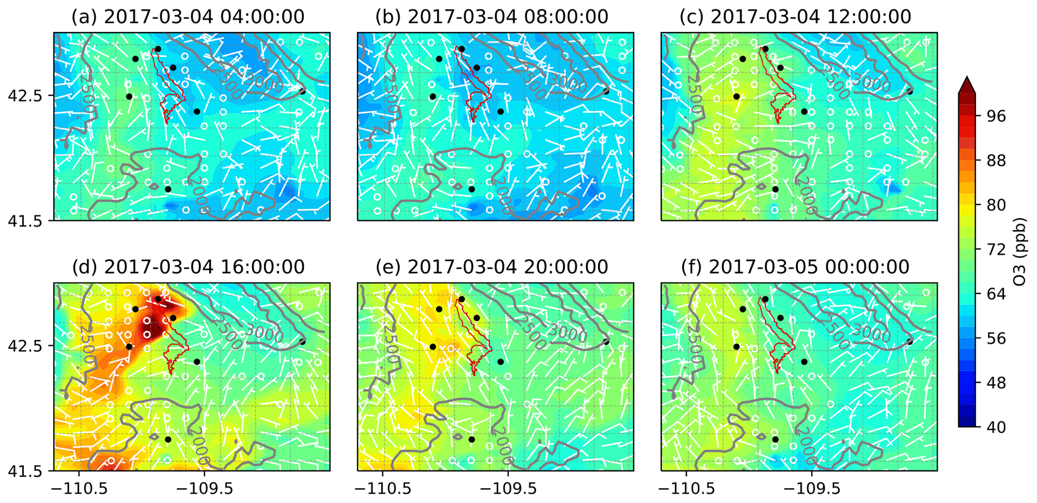
Figure 12 Simulated O₃ mixing ratios over the UGRB using RACM chemistry with dry deposition of gas species turned off (RACM_ddOff) for the O₃ event on 4 March 2017.

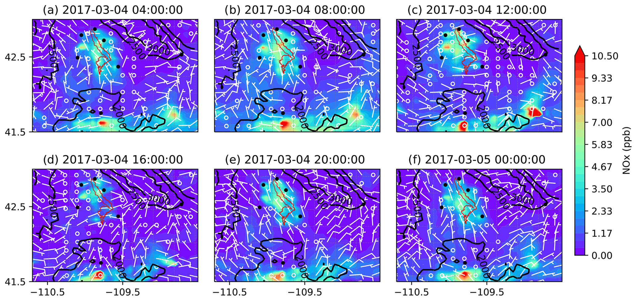
Figure 13 Similar to Fig. 12 but for NO_x mixing ratios.

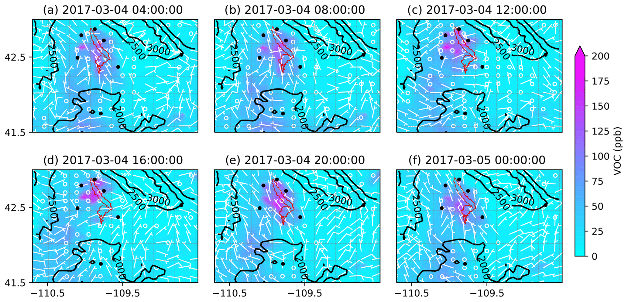
Figure 14 Similar to the Fig. 12 but for VOC mixing ratios.

The spatial variation in the formation and dissipation of O₃ and its precursors for the high-O₃ event on 4 March 2017 is shown in Figs. 9, 10, and 11 for O₃, NO_x, and VOCs, respectively, from the MOZ17 simulation, and similarly, Figs. 12, 13, and 14 show the results from RACM17. In both simulations, the formation and buildup of O₃ are seen around noon local time (Figs. 9c and 12c). In the late afternoon (at 16:00 LT), the O₃ mixing ratios reach their maximum of 124 ppb in MOZ17 (Fig. 9d) and 138 ppb in RACM17 (Fig. 12d). Although higher O₃ mixing ratios are found locally in RACM17, these dissipate rather quickly compared to MOZ17, demonstrating that there are subtle differences in the chemical mechanisms. For both simulations, the highest O₃ mixing ratios are seen closer to the Big Piney, Boulder, Daniel South, and Pinedale stations, though none of the stations are simulated to have the highest mixing ratios. If compared closely with the well locations in Fig. 1, the highest O₃ mixing ratios overlap the locations of the wells. The simulations with different chemical mechanisms show a similar temporal trend in O₃ formation, which can also be seen in Fig. 6, although the highest mixing ratios differ by approximately 10 ppb. The O₃ mixing ratios at Juel Spring, Moxa Arch, and South Pass are comparatively low. The wind speeds are also stronger (>5 m s⁻¹) around these stations (Figs. 9d and 12d). Particularly, near South Pass, the wind speeds are around 15 m s⁻¹. With the lack of mountains surrounding these stations and comparatively higher wind speeds, pollutant mixing ratios can be easily diluted and dissipated.

To better understand the formation, accumulation, and dissipation of O₃ precursors, i.e., NO_x and VOCs, the diurnal and spatial variations are shown for both simulations (Figs. 10, 11, 13, and 14). The simulations suggest that, as expected, most NO_x sources are in the production region for oil and gas, though the Pinedale results show that the inventory is missing some anthropogenic sources of NO_x, especially residential wood burning. The high mixing ratios of NO_x along the bottom of the figures are due to I-80 and not oil and gas infrastructure. Both chemical mechanisms show a similar trend in NO_x with the buildup of NO_x mixing ratios in the morning at 08:00 LT (Figs. 10b and 13b); higher mixing ratios at noon local time (Figs. 10c and 13c), which is a few hours before the higher mixing ratios of O₃ are simulated; and lower pollutant mixing ratios at 16:00 LT (Figs. 10d and 13d) when the O₃ mixing ratios are the highest. It is important to remember that the simulations underestimate the NO_x mixing ratios and the simulated NO_x mixing ratios do not vary largely among the simulations using different chemical mechanisms. Similarly to the diurnal variability in NO_x, the diurnal variability in VOCs from both simulations (Figs. 11 and 14) also shows a similar trend in the basin, with higher VOC mixing ratios occurring a few hours before the higher O₃ mixing ratios are simulated. Overall, the simulations capture the diurnal variation in O₃ and its precursors reasonably well. However, the simulated mixing ratios of the precursors are low compared to the respective observations, thus warranting further analysis into the sensitivity of simulated O₃ production to the precursor emissions.

4 VOC and NO_x sensitivity analysis

The results from the baseline simulations using both the MOZART and the RACM chemical mechanisms show that despite the low NO_x and VOC mixing ratios using the NEI2014v2 emissions, both models produce O₃ enhancements during the observed high-O₃ episodes. To understand the potential sensitivity of O₃ formation in the UGRB to VOC and NO_x levels, additional simulations were performed by comparing the baseline simulation results to observed VOC and NO_x mixing ratios and then adjusting the emissions by the ratio between the observed and modeled values, as outlined in Sect. 2.7. The factors used to adjust the emissions are shown in Table 5. The additional simulations for the sensitivity analysis all have dry deposition turned off, which is similar to the baseline simulations. Moreover, the data from the entire study period are used to adjust the NO_x mixing ratios because continuous NO_x data are available, as described in Sect. 2.7. It is clear from Table 5 that the model significantly underestimates all VOC species, thus requiring large emission enhancement factors to be applied to ensure that the model simulations produce VOC mixing ratios similar to the observations. More specifically, especially large adjustments are required for aromatic species. This result indicates that not only are the modeled VOC emissions too small but also the resulting mixture has lower-aromatic-species mixing ratios than what is observed, making the modeled VOC mixture significantly less reactive than the observed VOC mixture.

Table 5 Comparison of canister data from the Boulder station on 3 March 2017 collected between 04:00 and 07:00 LT and both MOZ17- and RACM17-simulated species for the same time period at the location of the Boulder station. The emission adjustment factors are computed by dividing the observed mixing ratios by the simulated mixing ratios for each species.

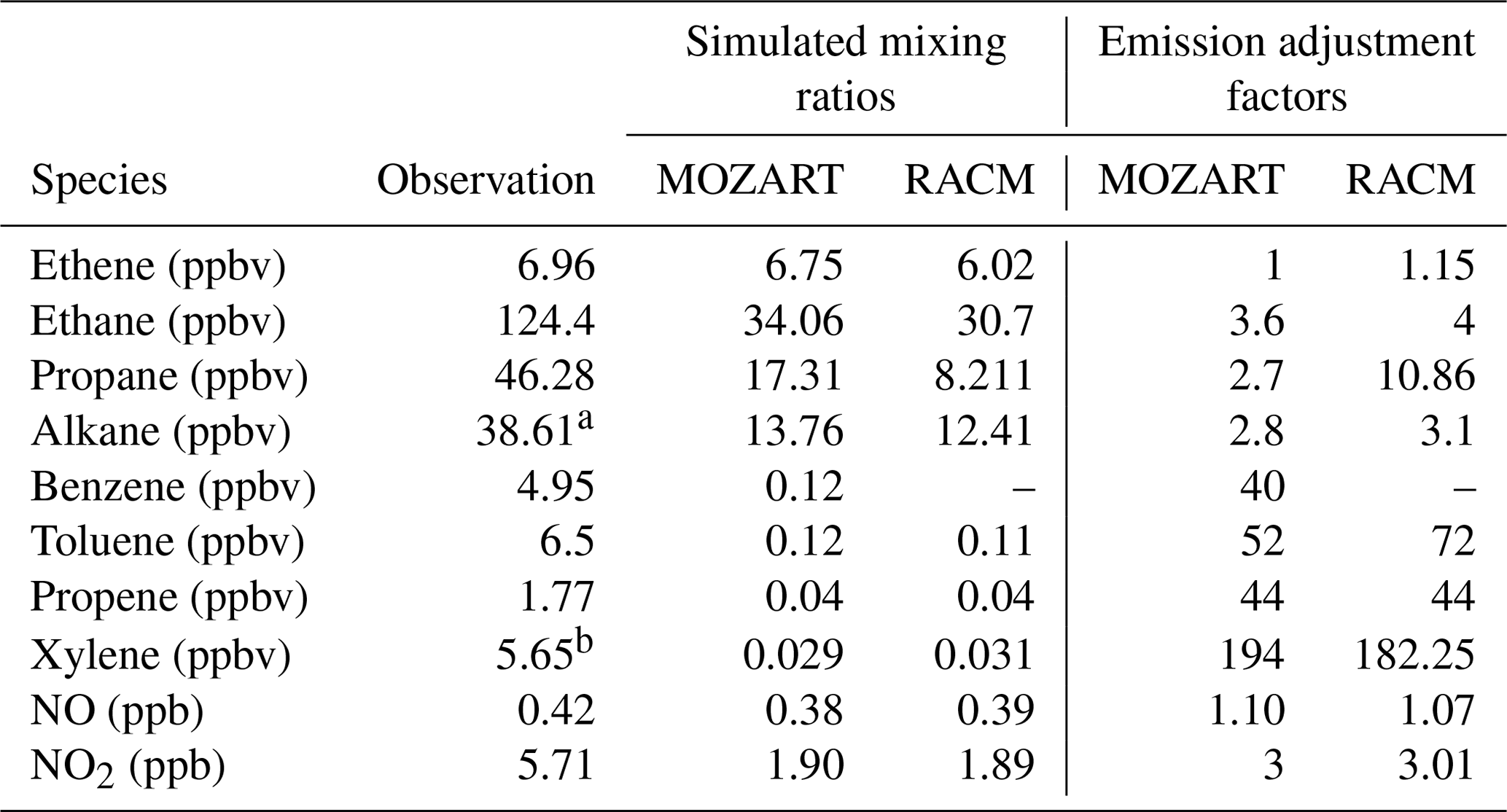
^a Sum of i-butane, n-butane, i-pentane, n-pentane, 2-methylpentane, 3-methylpentane, n-hexane, 2,4-dimethylpentane, 3-methylhexane, 2,2,4-trimethylpentane, n-heptane, 2-methylheptane, n-octane, n-nonane, n-decane, and undecane. ^b Sum of m- and p-xylene, o-xylene, 1,3,5-trimethylbenzene, and 1,2,4-trimethylbenzene.

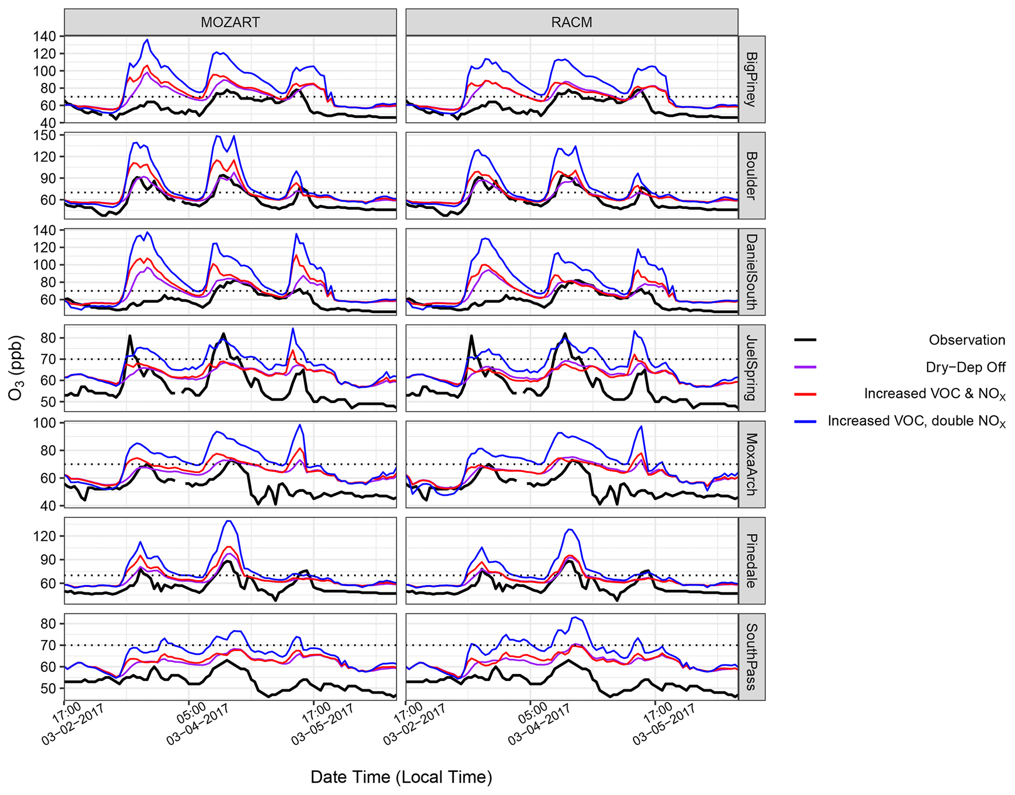
Figure 15 Time series of O₃ mixing ratios for the VOC and NO_x sensitivity simulations (red, increased VOC and NO_x; blue, increased VOC, double NO_x) at seven monitoring stations, along with the baseline simulation with dry deposition turned off. Note the different y scales for each station. Double NO_x refers to a doubling of the emission factors from Table 5.

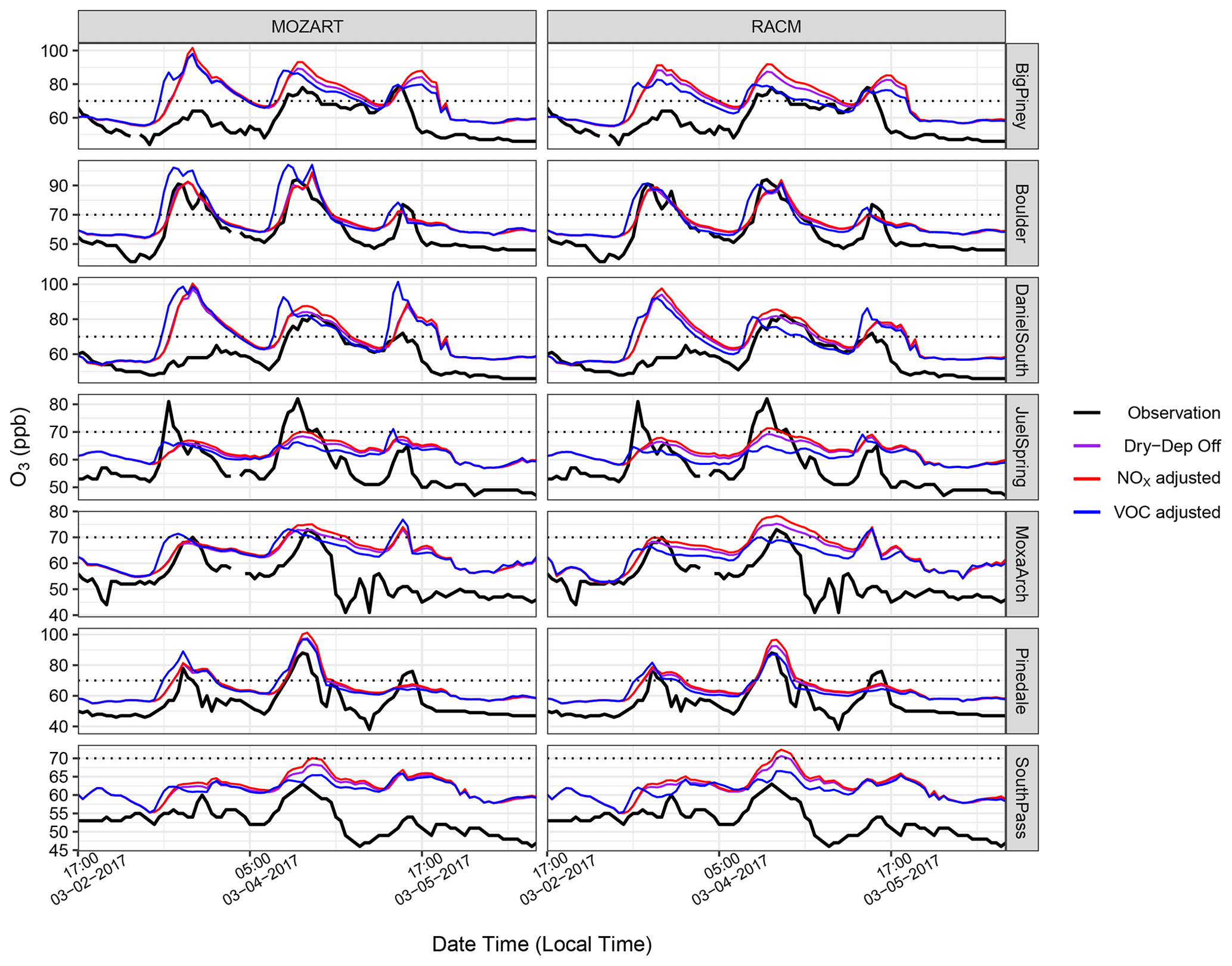
Figure 16 Similar to Fig. 15 but with only NO_x adjusted (red) and only VOCs adjusted (blue), along with the baseline simulation with dry deposition turned off. Note the different y scales for each station.

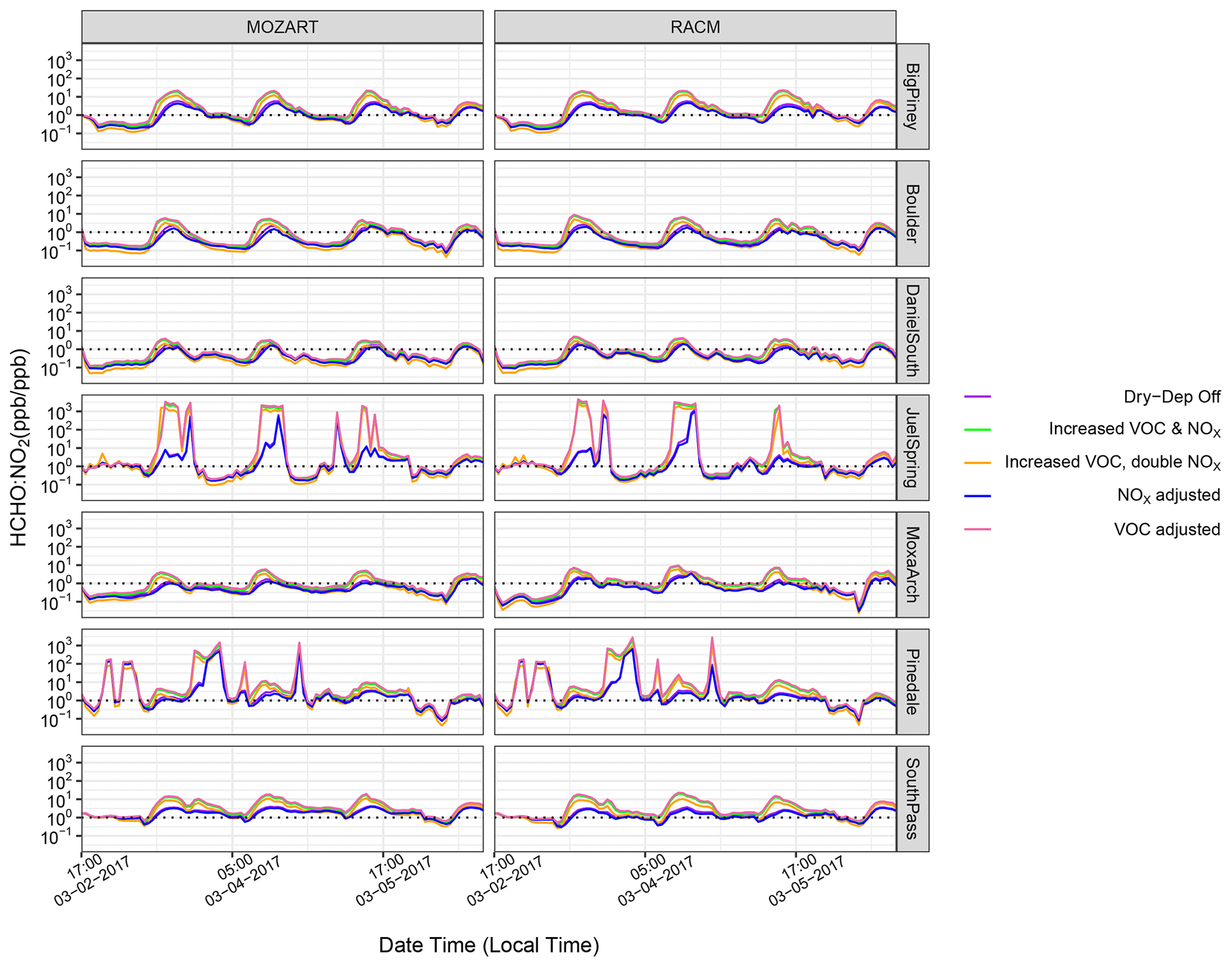
Figure 17 Time series of the HCHO : NO₂ ratio for the baseline simulations with dry deposition turned off (MOZ17 and RACM17; purple lines), as well as all of the sensitivity simulations at the seven monitoring stations. The dotted lines show the HCHO : NO₂ ratio of 1.

The O₃ mixing ratios from the aforementioned VOC and NO_x sensitivity simulations are shown in Figs. 15 and 16 and compared with data from the seven monitoring stations. Specifically, Fig. 15 shows the results for increased NO_x and VOCs compared to observed levels, which does increase O₃ formation but perhaps by less than would have been anticipated given the dramatic increases in VOC emissions and reactivity. In fact, these simulations do a good job of replicating the O₃ observed at the Boulder site in the RACM model while only moderately over-predicting O₃ formation with the MOZART mechanism. Further, an additional doubling of the NO_x emission adjustment factor causes a large jump in the O₃ predicted at all sites by both the RACM and the MOZART chemistry schemes. To explore the sensitivity to NO_x vs. VOC further, additional simulations were conducted where only NO_x and only VOCs were adjusted from the baseline simulation (Fig. 16). The simulation where only NO_x was adjusted results in moderate increases in the simulated O₃ mixing ratios at all sites and across the entire study period. When NO and NO₂ emissions were kept at their baseline levels and VOC emissions were adjusted, the simulations produce slight increases in O₃ at some sites, especially with the MOZART chemistry scheme, but at other sites the O₃ mixing ratios are not always elevated. Rather, in these cases, the timing of O₃ formation changes, with increases seen earlier in the day and sometimes even lower peaks in the modeled O₃ mixing ratio compared with the baseline simulation. These results are interesting and somewhat unusual, but further analysis was not pursued because by increasing VOCs while not adjusting NO_x, the VOC : NO_x ratio for this model simulation is far outside what is actually observed in the basin and is thus considered highly unrealistic. Altogether, these sensitivity simulations strongly suggest that O₃ formation in the basin is predominantly limited by the availability of NO_x rather than being controlled mainly by the VOC mixing ratios. Further, the results suggest that if more NO_x becomes available, the basin might see even higher levels of O₃ than currently observed. To further investigate this, the formaldehyde : NO₂ (HCHO : NO₂) ratio for all VOC and NO_x sensitivity simulations is presented in Fig. 17. This ratio has been used in previous studies as a proxy for VOC-limited and NO_x-limited conditions (Liu et al., 2021). Here, the ratio is well above 1 during the high-O₃ events for all simulations, with the only decrease being observed for the simulations with only increased NO_x emissions. These results further suggest that O₃ formation in the basin is strongly controlled by NO_x availability (Liu et al., 2021).

5 Conclusions

Over the past decade, there have been a number of elevated wintertime O₃ events in the UGRB, WY, with mixing ratios often exceeding 70 ppb. These events, though much less severe than observed a decade ago, have continued despite significant efforts to reduce emissions from oil and gas production. This fact drives the need for a photochemical model to better understand what is happening and to determine what emission reductions might effectively reduce O₃. This study, to the best of the authors' knowledge, is the first to utilize the EPA NEI2014v2 emission inventory with a fully coupled meteorology and chemistry model (WRF-Chem) to simulate O₃ events in the UGRB. The utilization of NEI2014v2 is key because this is the first NEI version to integrate non-point oil and gas sources, which are a dominant driver of the O₃ formation in the UGRB. Additionally, this study compared the results of two different chemical mechanisms (MOZART and RACM), focusing on their ability to reproduce the mixing ratios of O₃. Neither chemical mechanism can reproduce these high-O₃ events without modifying the default surface and photolysis albedo in the model. Furthermore, differences in dry deposition also affected the simulated accumulation of O₃, where the MOZART scheme accounts for dry deposition changes with snow cover while RACM does not. Thus, dry deposition was turned off to reduce inter-model differences, and these simulations produced similar amounts of O₃.

The model performance with regard to meteorology in the vertical was validated using vertical profiles of observed temperature during two IOPs from an earlier period (28 February to 2 March and 9 to 12 March 2011). Vertical data were only available from this time period. Although the simulated temperature was 2 to 4 ^∘C warmer than the observed temperature, the simulation captured the inversion layer near the surface. To validate the model's ability to predict the surface meteorology, 2 m temperatures and wind speeds from two WRF-Chem simulations (MOZ17 and RACM17) were compared with the observations at seven weather stations during the 2017 study period. The simulated 2 m temperatures showed a good correlation with observations at all stations. The simulated periods of low wind speeds also showed good agreement with the observed calm winds, though variability in the exact magnitude of the low winds results in relatively low correlation coefficients.

To study the model's ability to simulate high-O₃ events, we analyzed mixing ratios of O₃ and its precursors (NO_x and VOCs). The baseline simulations captured the high O₃ mixing ratios reasonably well at most of the stations, even though simulated levels of NO_x and VOCs were dramatically lower than observations. The low modeled mixing ratios of NO_x and VOCs suggest that emissions in NEI2014v2 are too low in the UGRB. Spatial plots of O₃ and its precursors show the predicted spatial extent of O₃ formation and that the models suggest the monitoring sites are close to, but not at, the location of maximum O₃. Sensitivity studies where the levels of NO_x and VOCs were increased to better match observations demonstrated that dramatically increasing VOC emissions and increasing the reactivity of the VOC mixture do not dramatically increase simulated O₃ mixing ratios. Rather, the O₃ levels appear to be predominantly controlled by NO_x availability. Because RACM has previously been shown to perform reasonably well at simulating O₃ events in the UB (Ahmadov et al., 2015) and again performs well in the current study when VOC and NO_x levels are adjusted to match observations, this study presents the possibility that O₃ might be able to be formed in the UGRB at significantly lower VOC levels than are currently observed.

Appendix A: Chemistry namelist options used for MOZART and RACM

Figures A1 and A2 present additional details regarding the WRF-Chem namelist options used in the MOZART and RACM simulations.

Figure A1 Namelist for chemistry options used for the simulations using the MOZART chemical mechanism.

Figure A2 Namelist for chemistry options used for the simulations using RACM.

Appendix B: Sensitivity analysis

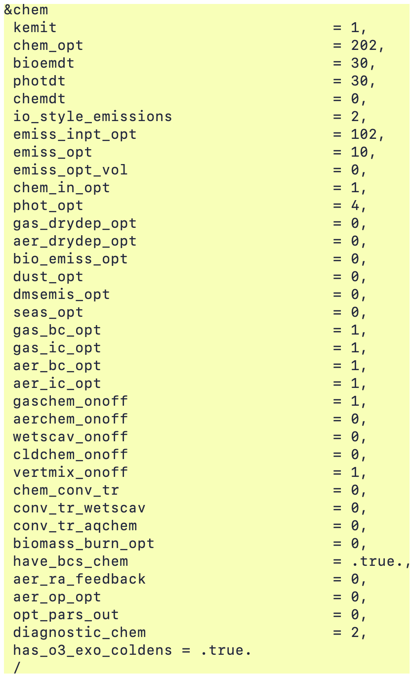
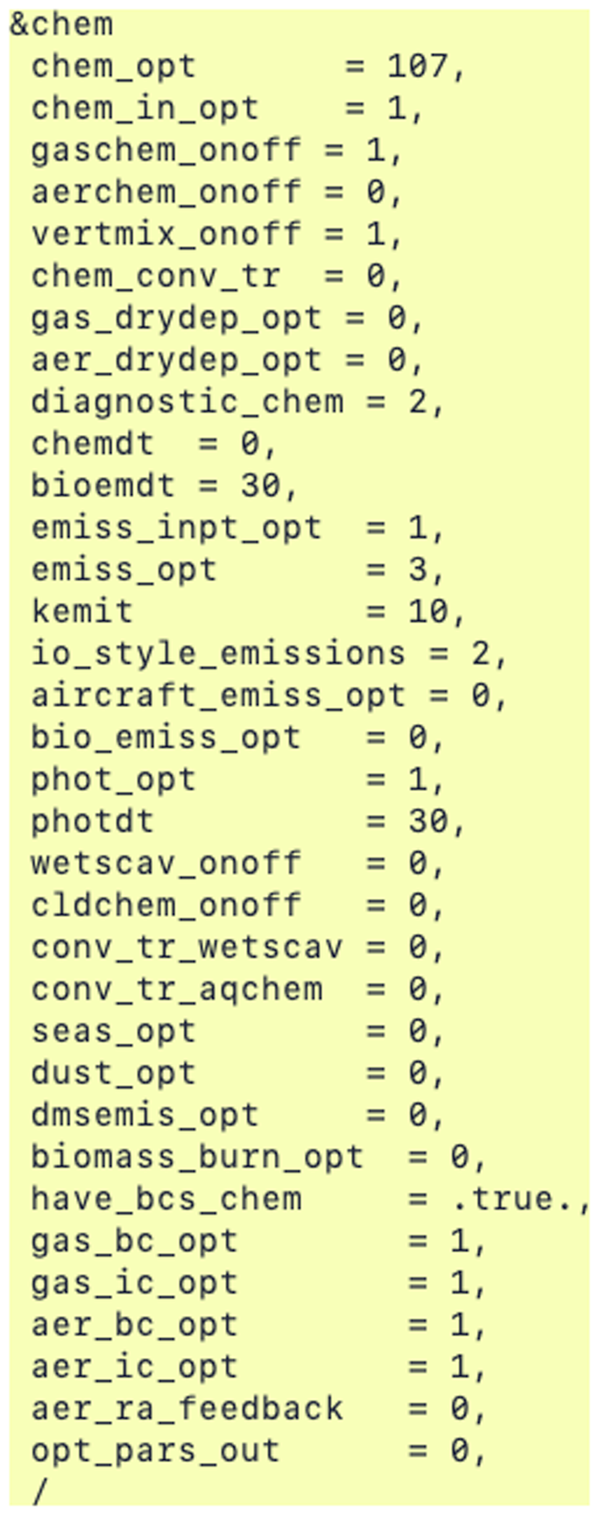
Table B1 presents ratios of observed VOCs and NO_x to simulated values at the four stations with speciated VOC observations. Note that the NO_x ratios are computed for the duration of the model simulation as shown in Fig. B1, whereas the ratios for the VOCs are only based on simulated means during the 4 h observation time window.

Table B1 Emission adjustment factor for four stations calculated based on the speciated canister data on 3 March 2017 collected between 04:00 and 07:00 LT and the baseline simulation (MOZ17 and RACM17).

Figure B1 Time series of observed and modeled NO and NO₂ at Boulder.

Appendix C: Additional data for Pinedale

To further demonstrate the model–observation disparity at the Pinedale location, which we attribute largely to wood burning emissions that are not included in the NEI dataset, Fig. C1 compares observed PM_2.5 and NO_x at Pinedale. The strong correlation is a good indicator that the high NO_x levels are related to the burning of wood that also causes enhanced PM_2.5.

Figure C1 Time series of PM_2.5 and NO_x observations at Pinedale.

Appendix D: Comparison with mobile laboratory data

Methane (CH₄) data from a Picarro cavity ring-down spectrometer (CRDS; model G2204) on board the University of Wyoming (UW) mobile laboratory (Robertson et al., 2020) were used to validate the CH₄ mixing ratios from the WYDEQ Boulder station. The CRDS was modified by Picarro Inc. to sample at 2 Hz. The National Institute of Standards and Technology (NIST) traceable (±1 %) CH₄ in an ultrapure air mixture with a CH₄ mixing ratio of 2.576 ppm was used to calibrate the Picarro instrument (Robertson et al., 2020).

Due to data availability, we compared the hourly CH₄ data from WYDEQ with the 1 s data from the UW mobile laboratory, as shown in Fig. D1. Only data from the time period over which the UW mobile lab was in the UGRB are shown, corresponding to 11:00 to 20:00 LT.

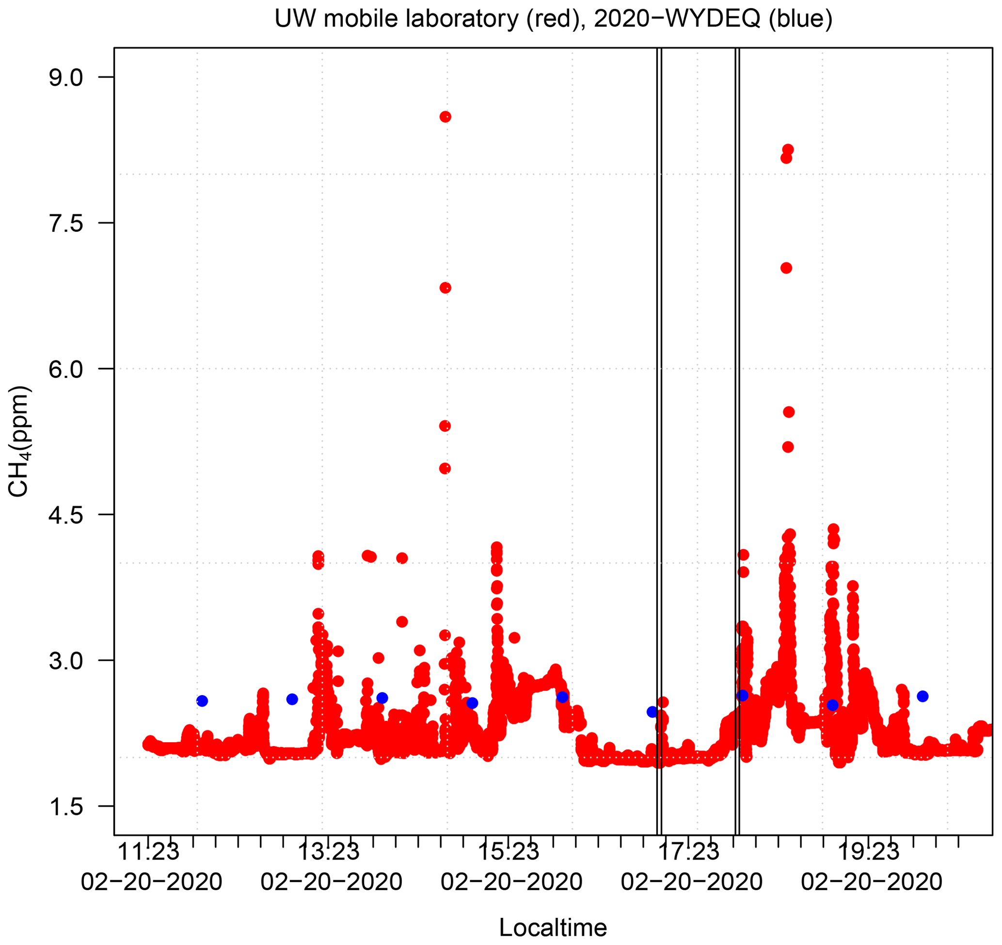
Figure D1 Time series comparison of CH₄ from the UW mobile laboratory (red) and WYDEQ Boulder site (blue) for 2 February 2020. The vertical black lines mark the times when the mobile laboratory was passing through the WRF grid box where the WYDEQ Boulder site is located.