the Creative Commons Attribution 4.0 License.
the Creative Commons Attribution 4.0 License.
 | 19 Jan 2023
Measurement report: Long-range transport and the fate of dimethyl sulfide oxidation products in the free troposphere derived from observations at the high-altitude research station Chacaltaya (5240 m a.s.l.) in the Bolivian Andes
Jiali Shen
Diego Aliaga
Samara Carbone
Isabel Moreno
Qiaozhi Zha
Wei Huang
Liine Heikkinen
Jean Luc Jaffrezo
Gaelle Uzu
Eva Partoll
Markus Leiminger
Fernando Velarde
Paolo Laj
Patrick Ginot
Paolo Artaxo
Alfred Wiedensohler
Markku Kulmala
Claudia Mohr
Marcos Andrade
Victoria Sinclair
Federico Bianchi
Dimethyl sulfide (DMS) is the primary natural contributor to the atmospheric sulfur burden. Observations concerning the fate of DMS oxidation products after long-range transport in the remote free troposphere are, however, sparse. Here we present quantitative chemical ionization mass spectrometric measurements of DMS and its oxidation products sulfuric acid (H2SO4), methanesulfonic acid (MSA), dimethylsulfoxide (DMSO), dimethylsulfone (DMSO2), methanesulfinic acid (MSIA), methyl thioformate (MTF), methanesulfenic acid (MSEA, CH3SOH), and a compound of the likely structure CH3S(O)2OOH in the gas phase, as well as measurements of the sulfate and methanesulfonate aerosol mass fractions. The measurements were performed at the Global Atmosphere Watch (GAW) station Chacaltaya in the Bolivian Andes located at 5240 m above sea level (a.s.l.).
DMS and DMS oxidation products are brought to the Andean high-altitude station by Pacific air masses during the dry season after convective lifting over the remote Pacific ocean to 6000–8000 m a.s.l. and subsequent long-range transport in the free troposphere (FT). Most of the DMS reaching the station is already converted to the rather unreactive sulfur reservoirs DMSO2 in the gas phase and methanesulfonate (MS−) in the particle phase, which carried nearly equal amounts of sulfur to the station. The particulate sulfate at Chacaltaya is however dominated by regional volcanic emissions during the time of the measurement and not significantly affected by the marine air masses. In one of the FT events, even some DMS was observed next to reactive intermediates such as methyl thioformate, dimethylsulfoxide, and methanesulfinic acid. Also for this event, back trajectory calculations show that the air masses came from above the ocean (distance >330 km) with no local surface contacts. This study demonstrates the potential impact of marine DMS emissions on the availability of sulfur-containing vapors in the remote free troposphere far away from the ocean.
- Article
(9274 KB) - Full-text XML
- BibTeX
- EndNote


Dimethyl sulfide (DMS), formed foremost from dimethylsulfoniopropionate (DMSP), which is produced by phytoplankton, is the primary natural contributor to atmospheric sulfur (Bates et al., 1992a; Simó, 2001; Lana et al., 2011). The estimated global DMS flux ranges from about 18 to 34 Tg S yr−1(Lana et al., 2011), which accounts for half of the natural global atmospheric sulfur burden (Simó, 2001). Undergoing a series of oxidation steps initiated by hydroxyl (OH), halogen, and nitrate (NO3) radicals, DMS contributes to aerosol particle formation and growth and thus to the formation of cloud condensation nuclei (CCN) via its oxidation products sulfuric acid (H2SO4) and methanesulfonic acid (CH3S(O)(O)OH, MSA) (Bates et al., 1992a; Charlson et al., 1987; Ayers et al., 1996). It has been estimated that DMS emissions contribute to 18 %–42 % of the global atmospheric sulfate aerosol. Therefore, more direct observations of DMS and also its oxidation products are needed to better understand the effects of DMS on climate (Szopa et al., 2021).
The DMS oxidation takes place via H abstraction or OH addition. The H abstraction and subsequent fast O2 addition leads to the peroxy radical . When reacts with RO2 or NO, it forms – via intermediates – the previously mentioned H2SO4 and MSA, participating in new particle formation, growth, and CCN formation processes (Covert et al., 1992; Beck et al., 2021). Both products have been detected many times in the marine atmosphere with a wide range of concentrations (Mauldin III et al., 1999; Berresheim et al., 2002; Bardouki et al., 2003; Baccarini et al., 2020; Beck et al., 2021). The reaction of with HO2 forms a hydroperoxide with the sum formula CH3SCH2OOH (Barnes et al., 2006). Recently, the autoxidation of was theoretically proposed and proven in lab experiments (Wu et al., 2015; Berndt et al., 2019; Ye et al., 2021). This pathway leads to the formation of hydroperoxy methyl thioformate (HPMTF; HOOCH2SCHO) that exists in concentrations of up to 50 pptv (1.25×10⁹ molecules cm−3) in the marine boundary layer (Veres et al., 2020). Other products of the abstraction channel are methyl thioformate (MTF, CH3SCHO) and methane sulfonic peroxide (CH3S(O)2OOH) that were detected in lab studies (Ayers et al., 1996; Barnes et al., 2006; Hoffmann et al., 2016; Ye et al., 2021; Berndt et al., 2019) but – to the best of our knowledge – not yet in ambient air.
In the addition channel, the first stable products are dimethylsulfoxide (CH3S(O)CH3, DMSO) and methanesulfenic acid (MSEA, CH3SOH). It is likely that MSEA reacts quickly with O3 to form SO2 (Berndt et al., 2020). DMSO reacts with OH, forming methanesulfinic acid (CH3S(O)OH, MSIA) alongside dimethylsulfone (DMSO2). DMSO2 has small chemical loss rates and has already been observed in the marine boundary layer in Berresheim et al. (1998). A recent cruise study over the Arabian Sea (Edtbauer et al., 2020) even reported concentrations of up to 120 pptv (3.0×10⁹ molecules cm−3) of DMSO2. Due to its long chemical lifetime, its formation and wet deposition rate control its concentration.
In this measurement report, we present data on DMS and its oxidation products in the tropical free troposphere over the Bolivian Andes; therefore we are now only focusing on previous free-tropospheric measurements. In high altitudes, >5000 m a.s.l., DMS concentrations are typically between 0 and 5 pptv (Simpson et al., 2001; Thornton et al., 1992) but can drastically exceed 5 pptv close to convectional updrafts (Thornton and Bandy, 1993; Thornton et al., 1992). Nowak et al. (2001) measured dimethylsulfoxide (CH3S(O)CH3, DMSO) concentrations of about 5 pptv in the tropical marine free troposphere at approximately 1500 m a.s.l. Mauldin III et al. (1999) and Zhang et al. (2014) reported very variable gas-phase MSA concentrations, reaching unexpectedly high values up to 1×108 cm−3 above 8000 m a.s.l. and 2×107 cm−3 at 2500 m a.s.l., respectively, under very dry conditions. Both reported MSA evaporation from aerosols as a plausible source. Unfortunately, no pressure or pressure corrections were mentioned in both publications, so we can not directly compare our data to these former measurements. Veres et al. (2020) detected rather low concentrations of HPMTF in the upper troposphere. Other DMS oxidation products such as DMSO2, MSIA, or MTF, have – to our knowledge – not been observed in the free troposphere. This is probably due to their low concentrations caused by dilution, oxidation, and partitioning onto aerosols and into cloud water, which challenges analytical instrumentation.
In the tropical upper troposphere over the oceans, new particle formation (NPF) has been observed by in situ aircraft measurements (Williamson et al., 2019), and global models suggest that the particle formation at these altitudes typically involves H2SO4 (Dunne et al., 2016; Gordon et al., 2017). DMS oxidation is partly responsible for the involved H2SO4, especially over remote marine areas and in the vicinity of convective updrafts (Thornton et al., 1992). Froyd et al. (2009) detected acidic aerosols in the free troposphere at an altitude of 4–12 km that originated from convective updrafts over the Pacific and remained in the atmosphere for days up to even weeks during the CR-AVE flight campaign southwest of Central America. The aerosols with diameters ≥0.5 µm, analyzed by laser mass spectrometry (PALMS, Thomson et al., 2000), contained a large fraction of methanesulfonate (MS−), which links them to DMS oxidation. In contrast to MSA, H2SO4 can also have other sources, such as anthropogenic or volcanic SO2, which react with OH in the presence of water vapor to form H2SO4.
Our measurements took place at the high-altitude Global Atmosphere Watch (GAW) station at mount Chacaltaya (CHC), located in the Bolivian Andes at 5240 m a.s.l. Particle formation and growth events occur regularly at CHC during daytime (onset ca. 10:00 local time) with the highest NPF frequencies in May at the beginning of the dry season (Rose et al., 2015). Especially under westerly wind conditions nearly 100 % of the days had particle formation events. Rose et al. (2015) hypothesized that particle formation occurs after the mixing of clean oceanic free tropospheric air masses with continental air from up-slope winds and convective updrafts. They suggest that the former provides a low-condensation-sink background thus favoring particle formation, and the latter contains the required condensable vapors. However, gas- and particle-phase composition data of air masses from the free troposphere (FT) and continental boundary layer (BL) during the different seasons and wind directions were missing. Possible sources for such condensible vapors in the southwest to the northwest of the station are volcanic outgassing on the Altiplano (a large semi-arid plateau in the Andes), the close-by metropolitan area La Paz and El Alto, or the 75 km distant southern shores of Lake Titicaca during the day, while the Pacific coast is 330 km away from the station. The intensive measurement campaign Southern Hemisphere High Altitude Experiment on Particle Nucleation and Growth (SALTENA) (Bianchi et al., 2021), lasting from the end of December 2017 to the beginning of June 2018, was planned to improve our understanding of the chemistry behind the observed new particle formation. With the Amazon basin to the east and the open Pacific to the west, the air mass composition reaching CHC in the wet and dry seasons is likely very different, as the prevalent wind direction shifts from the lowlands in the east during the wet season to the west during the dry season.
For this study, we focused our analysis on data obtained in May 2018, when the wind came foremost from the direction of the Pacific Ocean and the Altiplano (southwest to northwest), and blue-sky conditions were prevalent as typical for the dry season at the Bolivian Altiplano. Our aim was to quantify condensible vapors and possibly their precursors in air masses reaching CHC via long-range transport in the tropical free troposphere that originated from the Pacific, using an array of state-of-the-art instruments. We present simultaneous measurements of DMS and its oxidation products H2SO4, MSA, DMSO, DMSO2, MSIA, MTF, CH3S(O)2OOH, and CH3SOH, as well as measurements of sulfate and methanesulfonate aerosol mass fractions, at CHC. The variety of sources and air masses influencing the air composition at CHC (e.g., Bianchi et al., 2021; Rose et al., 2015; Wiedensohler et al., 2018; Achá et al., 2018) required a careful distinction of air masses impacted by local emissions and long-range transport, which we present in the results, using strict thresholds for typical markers of local urban emissions in agreement with the FLEXible PARTicle dispersion model (FLEXPART). We test this distinction by analyzing the observations of different instruments in different air masses. In this context, a measurement of the ion composition of the different air masses in a completely different month but under comparable conditions deserves special mention. We then discuss DMS chemical conversion to its oxidation products during transport, considering both their gas-phase and particle-phase concentrations. With our measurements at CHC we hope to shed some light on the DMS oxidation and transport in the free troposphere by contributing measurements of most DMS oxidation products at such an altitude.
2.1 Measurement location and potential sources of DMS
The measurements took place at the Chacaltaya (CHC) Global Atmosphere Watch (GAW) station which is located east of the Altiplano close to the main ridge of the Bolivian Andes ( S, W, 5240 m a.s.l.; see Fig. B1 in Appendix B for the elevation data) and 330 km away from the Pacific coast. The area is semi-arid and partly covered by snow, especially after precipitation events. The vegetation on the Altiplano is dominated by tufts of hard grass on which local farmers let their llamas graze. The metropolis La Paz and El Alto, located 17 km south of Chacaltaya GAW station with an elevation ranging from 3300–4100 m a.s.l., is an important source of anthropogenic emissions impacting CHC.

Figure 1The location of the Chacaltaya (CHC) GAW station with a focus on potential DMS emission hotspots in the region. The color code shows the average chlorophyll concentration in the Pacific Ocean and Lake Titicaca for May 2018 as obtained from satellite data (Aqua MODIS). All lagoons, also those for which no chlorophyll data are available, are marked with dark blue outlines. The horizontal extent of the model domain for backward Lagrangian calculations (see Sect. 2.4.1 for details) is depicted as a dashed pink line.
The southern part of Lake Titicaca (Lago Menor) lies about 75 km away to the west and northwest of the station, as can be seen in Fig. 1. Lake Titicaca, which is the largest freshwater lake in South America with a surface area of 8372 km2, experienced its first algal bloom in 2015. The algal bloom occurred due to anthropogenically increased nutrient levels after climatologically extreme rain events (Achá et al., 2018). These rain events and subsequent algal blooms will likely become more frequent in the future and impact especially the shallow and nitrogen-rich Lago Menor (Duquesne et al., 2021) at the south end of Lake Titicaca. The algal bloom in the year 2015 involved green algae of the Carteria species (Achá et al., 2018), known to produce DMSP (Franklin et al., 2010) and DMS (Andreae, 1980). Other lagoons on the Altiplano that might host algae and thus emit DMS lie a few hundred kilometers to the south. To evaluate the possible impact of these potential local sources on signals of marine trace gases, we used backward Lagrangian dispersion calculations (Aliaga et al., 2021). Figure 1 shows the horizontal radial extent (1600 km) of the model domain; a detailed description follows in Sect. 2.4. A description of the continuous long-term measurements from the GAW station that we used in this study can be found in Sect. 2.3.
2.2 The SALTENA campaign
Advanced field measurements with an extensive suite of novel gas and particle composition instruments at CHC were conducted between December 2017 and the beginning of June 2018 (SALTENA, Bianchi et al., 2021). The aim of the campaign was to determine the chemical species of anthropogenic and biogenic origin impacting the station and contributing to new particle formation.
Atmospheric ions were detected by the Atmospheric Pressure interface-Time of Flight mass spectrometer (Positive-APi-TOF, Sect. 2.2.6) and the gas-phase composition by a nitrate chemical ionization atmospheric-pressure-interface time-of-flight mass spectrometer (nitrate-CIMS, Sect. 2.2.1), a filter inlet for gases and aerosols (FIGAERO) coupled to a high-resolution time-of-flight chemical ionization mass spectrometer using iodide chemical ionization (I−-FIGAERO-CIMS, Sect. 2.2.4), as well as a proton transfer reaction time-of-flight mass spectrometer (PTR3, Sect. 2.2.2). The Quadrupole Aerosol Chemical Speciation Monitor (Q-ACSM, Sect. 2.2.5) and the I−-FIGAERO-CIMS further analyzed the aerosol particle composition. Table 1 summarizes which of the analyzed species are detected by which instrument. An overview of the operation times of the instruments and the herein presented periods is given in Fig. 2.
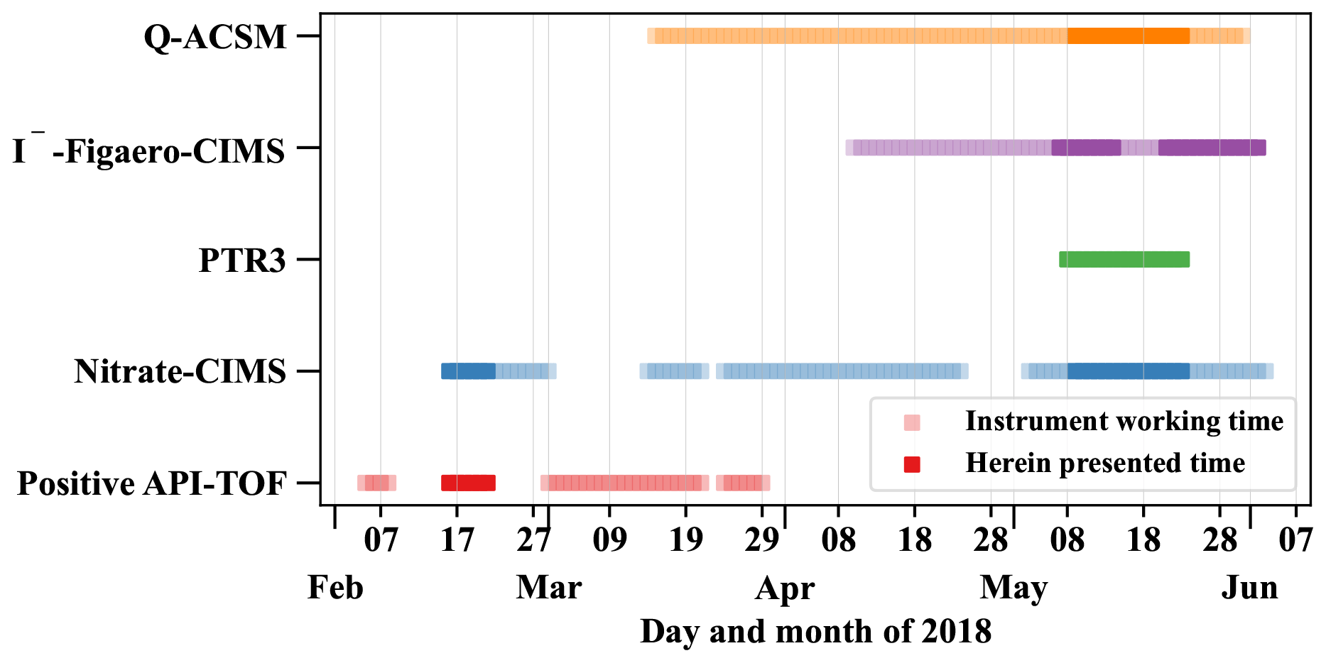
Figure 2Overview of the operation times of the individual mass spectrometers and the herein presented time periods. The herein presented times are chosen by filtering for typical dry season conditions (westerly winds, clear sky) and removing all periods with uncertain data quality, e.g., due to technical difficulties and power cuts.
Table 1An overview of the mass spectrometers used during the SALTENA campaign and their respective detected species.

2.2.1 Nitrate-CIMS
The nitrate-CIMS (TOFWERK AG, Thun, Switzerland) measured the concentration of H2SO4, MSA, and a compound with the exact mass of CH3S(O)2OOH from 19 to 25 April and 5 May to 3 June. The specially designed inlet for chemical ionization at ambient pressure is described by Kürten et al. (2011) and Jokinen et al. (2012). The data we report here are averaged for 10 min. The nitrate-CIMS uses nitrate anions [(HNO3)n (NO), n=0–2] as reagent ions to ionize gas molecules (M) via proton transfer from the molecule to the nitrate ions or by ligand switching reactions, forming clusters.
The signal of the detected compound in counts per second (cps) is normalized to the sum of count rates of reagent ions and then multiplied with the calibration coefficient C. The calibration coefficient cm−3 was determined after the campaign, using H2SO4 as calibrant, following the procedure by Kürten et al. (2012). We assume the effect of temperature and humidity on charging efficiency to be negligible. Due to the lack of standards, we could not calibrate every individual species we detected. Therefore, we use the H2SO4 calibration factor C to estimate MSA and CH3S(O)2OOH concentrations. The sampling flow was 10 slpm, mixed with 20 slpm sheath flow before measurement. The inlet is a 150 cm long stainless steel tube with a 1.905 cm inner diameter, and its line loss for H2SO4 is already included in the calibration factor.
2.2.2 PTR3
The PTR3 ionizes sample gas molecules with (H2O)nH3O+ clusters mainly via ligand switching (H3O+-mode) and detects volatile organic compounds (VOCs) and their oxidation products. It has been described previously by Breitenlechner et al. (2017). During the SALTENA campaign, the length and diameter of the inlet were 90 cm and 10 mm, respectively. Core sampling right before the ion-molecule reaction region, subsampling only 1.2 out of 7.5 slpm air, reduces inlet wall losses to approximately 55 % as calculated from laminar transport and radial diffusion. From 8 to 23 May 2018 we used a radio frequency sinusoidal voltage with an amplitude of 400 V peak-to-peak at a pressure of 55 mbar and a temperature of 310 K, corresponding to an (E: electric field and N: concentration of neutral particles) of 106±25 townsend (Td), leading to primary ion distributions as shown in Fig. C1 in Appendix C1. Compounds with proton affinities above ∼200 kcal mol−1, like hexanone or DMSO, are ionized at the kinetic limit. Those with lower proton affinities need to be calibrated individually, which is, e.g., the case for DMS. During the campaign we calibrated the PTR3 regularly by mixing 7.5 sccm of nitrogen 5.0, containing 1 ppm of hexanone (98 %), 1,2,4-trimethylbenzene (98 %), alpha-pinene (≥99.9 %), and acetonitrile (≥99.9 %), each, as reference standards (all purchased from Sigma-Aldrich), into 7.5 slpm of compressed air with purity 5.0. Hexanone is our reference for compounds ionized at the limit of detection in the H3O+ mode and gives us the maximally possible sensitivity for a sample gas molecule. To lower the limit of detection, we averaged the data to a 5 min time resolution.
2.2.3 Quantification of gas-phase DMS and its oxidation products detected by the PTR3 and nitrate-CIMS
For DMS, detected by the PTR3, we performed water-vapor-mixing-ratio-dependent off-site calibrations after the campaign together with acetonitrile (nearly daily on-site calibrations available) as a reference. The calibration curves are shown in Fig. C2 in Appendix C1. The DMS time series was then calibrated, using the humidity-dependent calibration function, multiplied by a time-dependent transmission factor that we inferred from the comparison of the regular acetonitrile calibrations at their respective humidity with its humidity-dependent calibration curve. For DMS (calibrated), MSIA, DMSO, and DMSO2 (ionized at the kinetic limit in H3O+ mode; see Shen et al., 2022) we have good references and can therefore assume a low uncertainty of the concentrations of around 30 %. For all other oxidized organosulfur compounds observed by the PTR3 of which proton affinities are typically unknown, we assumed a sensitivity at the kinetic limit so that their presented concentrations are lower-limit estimates.
Analogous to H2SO4, MSA, detected by the nitrate-CIMS, has a collision-limited charging efficiency when reacting with the nitrate ions, resulting in strongly bound clusters not prone to fragmentation. It is therefore valid to use the H2SO4 calibration factor. However, we can only give the lowest estimated concentration for CH3S(O)2OOH due to its low detection efficiency (Shen et al., 2022).
Small signals close to the detection limit or background (e.g., due to neighboring peaks) make the quantification more difficult.
To discuss the impact of the limit of detection on the data quality of some important compounds, we present lower-limit concentration distributions of detected organosulfur compounds from the PTR3 and nitrate-CIMS together with their limits of detection in Fig. C3 in Appendix C2. The limit of detection also takes the maximum amount of interference by neighboring peaks into account. Apart from DMSO and DMSO2, all of the compounds frequently exhibited low concentrations close to the detection limit, so their concentrations are somewhat uncertain during such times. In our analysis, however, we focus on periods when the signals were typically higher than their median and thus higher than their respective limit of detection. The peaks are clearly visible and quantifiable under these circumstances. All concentrations reported are given in molecules cm−3 for standard conditions.
2.2.4 I−-FIGAERO-CIMS
The I−-FIGAERO-CIMS (Aerodyne Research, Inc.) was deployed to measure the molecular composition of both gas-phase and particle-phase organic compounds and inorganic acids. The FIGAERO inlet has two modes. In the gas-phase mode, ambient air was directly sampled into the ion-molecule reactor while particles were simultaneously collected on a 25 mm Zefluor polytetrafluoroethylene filter through another sampling port with a flow of 3.8 slpm. The duration of particle-phase sampling was 120 min. When the gas-phase measurement (particle-phase sampling) was completed, the FIGAERO inlet was switched to the particle-phase mode, and a nitrogen gas stream (2 slpm) was heated and blown through the filter to evaporate the particles via temperature-programmed desorption. More details about the instrument can be found in Lopez-Hilfiker et al. (2014) and Thornton et al. (2020). The instrument was working from 10 April to 2 June 2018 with only short interruptions due to power outages. From 14 to 21 May no particle-phase, but only gas-phase data are available.
2.2.5 Q-ACSM
The Quadrupole Aerosol Chemical Speciation Monitor (Q-ACSM, Aerodyne Research, Inc.) (Ng et al., 2011) measured the non-refractory submicron aerosol components: organics, nitrate, sulfate, ammonium, and chloride. To remove larger particles to avoid clogging the Q-ACSM inlet, a PM2.5 cyclone was integrated in the inlet. The Q-ACSM was calibrated with ammonium nitrate and sulfate, following the recommendations of Ng et al. (2011), who also described the instrument in further detail. The time resolution of the Q-ACSM was 30 min. In this study, we use the data from the Q-ACSM collected during 9–23 May 2018.
2.2.6 Positive-APi-TOF
The Atmospheric Pressure interface-Time of Flight (APi-TOF) mass spectrometer was operated in positive ion mode to detect positively charged ions and ion clusters from February to March 2018. From April to June, we switched the Positive-APi-TOF to the negative mode for measuring negatively charged ions and ion clusters. A detailed description of the instrument and operation can be found in Junninen et al. (2010). We used 20 min averages when pre-processing the data. The total inlet flow was kept constant at ∼14.5 slpm of which 0.8 slpm was analyzed by the instrument to minimize losses of ions to the inlet walls. The inlet line was a stainless steel tube of 1 cm inner diameter and ∼ 100 cm length.
2.3 Long-term measurements at CHC
The data from the SALTENA campaign were analyzed in the context of the data from the continuous measurements taking place at the GAW station, which is equipped with standard instruments to measure trace gases like CO and CO2, for example. An automatic weather station (AWS) deployed at the station records air temperature, relative humidity, radiation, wind direction, and wind speed at a 1 min resolution. Aerosol physical, chemical, and optical properties have been measured nearly continuously in the past 10 years. The aerosol particle size distribution is monitored with a mobility particle sizer spectrometer (MPSS), assembled with the TSI Inc. 3772 Condensation Particle Counter and a custom-made differential mobility analyzer. The MPSS measures the particle size distribution in the range of 10 to 650 nm with a 5 min time resolution. A multi angle absorption photometer (MAAP) monitors the equivalent black carbon (eBC) mass with a time resolution of 1 min (Petzold et al., 2005). The data are reported at standard temperature and pressure conditions, following the GAW network recommendations (WMO and GAW, 2016), and the data are corrected considering the effective wavelength of the instrument in accordance with Müller et al. (2011).
Two interchangeable digital impactors are used to collect the aerosol particulate matter with aerodynamic diameters lower than 10 and 2.5 µm (i.e., PM10 and PM2.5, respectively). The collectors are equipped with pre-baked quartz fiber filters (Ø 150 mm) collecting samples at a flow rate of 30 m3 h−1. The filters are exchanged once a week and are analyzed by a Dionex Ion Chromatograph, Sunset Laboratory total organic carbon analyzer (applying the EUSAAR_2 protocol; Cavalli et al., 2010) and by high-performance liquid chromatography coupled to a pulse amperometric detector to determine the ions, organic and elemental carbon, and anhydrous monosaccharides. We use data of methanesulfonate from December 2011 to August 2017. A more detailed description of the site and further long-term measurements can be found in previous studies (Wiedensohler et al., 2018).
2.4 Analysis of air mass history
Aliaga et al. (2021) used a high-resolution meteorological model coupled with Lagrangian dispersion calculations to identify where air masses sampled at CHC originate from and to quantify the relative influence of the surface and the free troposphere. Here we utilize, and further analyze, the output from the same simulations (Aliaga, 2021).
Aliaga et al. (2021) performed a 6-month-long simulation with the Weather Research and Forecast (WRF) model. The simulation had four nested domains. The outermost and largest domain had a grid spacing of 38 km, whereas the innermost domain, covering the area closest to CHC, had a grid spacing of 1 km. The meteorological output of the WRF simulation was saved every 15 min and used as input to the Lagrangian dispersion model FLEXible PARTicle dispersion model (FLEXPART). The high temporal and spatial resolution of the driving meteorological data is a key advantage over dispersion or trajectory simulations driven by reanalysis data – typically only available every 1 to 6 h. Backward dispersion simulations were performed with FLEXPART. For every hour, 20 000 particles were randomly distributed and then released from a 10 m deep (a.g.l) layer covering a 2×2 km square centered on CHC. The trajectories of all particles were tracked back in time for 4 d. It should be noted that the particles were treated as passive tracers that do not undergo any chemical or microphysical processing.
The output of FLEXPART is the source–receptor relationship (SRR), which is related to the particles' residence time in the 3-dimensional grid cells of the FLEXPART output grid. Aliaga et al. (2021) transformed the SRR output from the Cartesian grid to a log-polar grid so that the size of the grid cells gradually increases with the distance from CHC (the receptor); additional details of this transformation, and its motivation, are provided in Aliaga et al. (2021). The domain of the log-polar grid is a cylinder covering an area with a radius of 1600 km centered on Chacaltaya (Fig. 1 shows its horizontal extent) and reaching from the surface to 15 km a.g.l.
As the FLEXPART domain is limited in size, it is possible that during the 4 d of backwards travel particles can leave the domain. Therefore, unlike in Aliaga et al. (2021), we also estimated the amount of air masses arriving at CHC originating from outside the FLEXPART domain (herein referred to as “out of domain”). Similar to Aliaga et al. (2021), we identified air masses arriving from different pseudo layers within the FLEXPART domain (referred to as “within domain”): surface layer (air masses from the lowest FLEXPART output layer 0–500 m a.g.l.), boundary layer (air masses from below 1500 m a.g.l.), and free troposphere (air masses from above 1500 m a.g.l.).
The out-of-domain air mass contribution is computed as follows: theoretically, if all particles remained in the domain, the domain-integrated SRR would be 4 d. However, in the case when particles leave the domain, the domain-integrated SRR is less than 4 d. The out-of-domain SRR is therefore computed as the theoretical maximum SRR minus the actual SRR. No information is available about the trajectories of the particles once they have left the domain.
Footprint analysis
To identify the specific source regions of chemical species measured at CHC, the SRR from FLEXPART can be combined with the in situ measurements of such species via an elastic net regression (Pedregosa et al., 2011). The same method was used to identify likely sources of black carbon measured at CHC (Bianchi et al., 2021). In contrast to Bianchi et al. (2021); however, we also included the lateral boundaries of the FLEXPART domain in the footprint analysis to visualize the long-range transport into the domain through these boundaries.
3.1 Determining free tropospheric periods under typical dry season conditions
To identify periods dominated by free tropospheric (FT) air masses versus periods dominated by boundary layer (BL) emissions, we present a compilation of important measurements (all reported for standard conditions) in Fig. 3. The time series of gas-phase MSA is shown in Fig. 3a), as well as the sum of C8H10Ox compounds, which are likely oxidation products of aromatic xylenes or ethylbenzene, and we can thus use them as indicators for anthropogenic emissions (e.g., Li et al., 2019). It is noticeable that gas-phase MSA is high whenever C8H10Ox is low, as shown more clearly in Fig. D4 in Appendix D1.
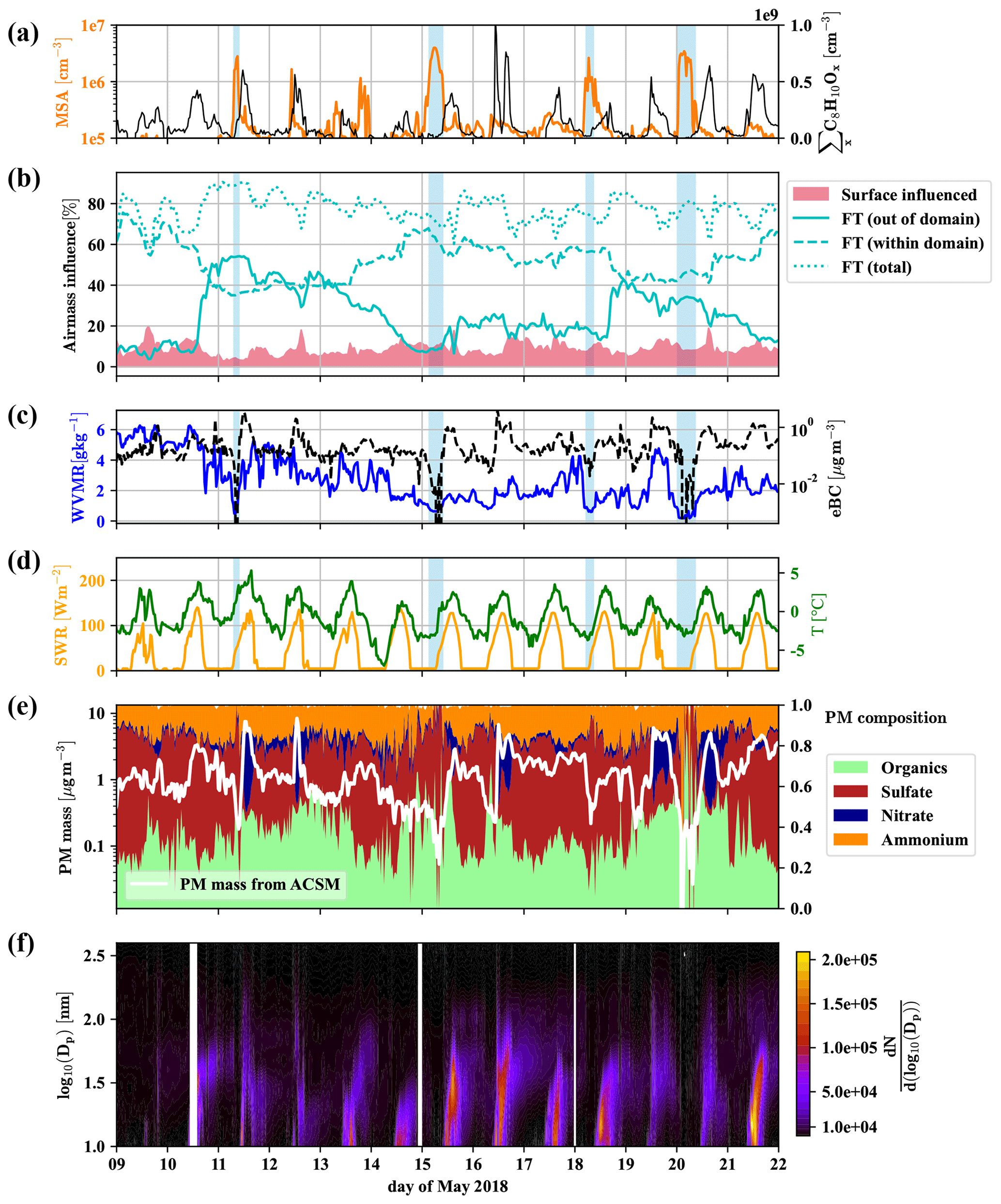
Figure 3Overview of 2 weeks of data for the identification of free tropospheric periods. Methanesulfonic acid (MSA) and summed C8H10Ox (a), the influence of surface (<500 m a.g.l.) and free tropospheric air masses (>1500 m a.g.l.) according to FLEXPART, with free tropospheric (FT (total)) air masses shown additionally divided into the air from within and without the FLEXPART domain (b), water vapor mixing ratio (WVMR, solid) and equivalent black carbon mass (eBC, dashed) (c), shortwave radiation (SWR) and temperature (T) (d), particle matter (PM) mass and composition from the Q-ACSM (e), and particle number distribution () (f) versus local time. Light blue shaded areas mark times that we consider dominated by free tropospheric air masses due to the low particle load and water vapor mixing ratio.
Figure 3b shows the amount of air coming from the free troposphere (>1500 m a.g.l.) and influenced by surface emissions (0–500 m a.g.l.) according to the results of the FLEXPART Lagrangian dispersion analysis. Furthermore, we show the fractions of free tropospheric air from out of the FLEXPART domain and within the domain (defined in Sect. 2.4).
We also present the water vapor mixing ratio (WVMR) and equivalent black carbon mass (eBC) (Fig. 3c), shortwave radiation (SWR) and temperature (Fig. 3d), the Q-ACSM total particle mass and its composition (Fig. 3e), followed by the particle number size distribution (Fig. 3f).
Figure 3b reveals that free tropospheric air masses reach the CHC GAW station all the time during the period shown. However, neglecting the varying boundary layer height in these traces (see Aliaga et al., 2021, Sect. 4 for a justification of the differentiation using constant pseudo layer heights instead of a time-resolved boundary layer height) leads to a tendency to underestimate the surface influence during daytime and the free tropospheric air during nighttime (when the inversion is below 1500 m a.g.l.). Especially during the daytime, free tropospheric air mixes with local air masses from the surface layer (spikes in the surface layer influence in Fig. 3b). This leads to enhanced concentrations of the anthropogenically emitted C8 compounds (Fig. 3a), as well as a larger nitrate fraction in the particle mass (Fig. 3e). We observe particle formation events nearly every day as previously reported by Rose et al. (2015), typically followed by particle growth that regularly extends into the night and sometimes without interruption (e.g., 15–16, 16–17 May 2018) until the next particle formation event the next day (Fig. 3f). However, during certain periods (marked by blue shadings in Fig. 3), at late night or early morning, when the temperature reaches its daily minimum, eBC (Fig. 3c) and the particle mass determined by the Q-ACSM (Fig. 3e) show a sudden drop, coinciding with overall lower particle numbers measured by the MPSS (Fig. 3f; see also Fig. D2 in Appendix D1 for the number size distribution) and particularly low water vapor mixing ratios (Fig. 3c). These are strong indications that the station was above the shallow boundary layer of the Altiplano and that free tropospheric air masses had subsided from higher altitudes.
The FLEXPART dispersion simulation can resolve this, as shown in Fig. 4 for 11 May; as an example: during the whole day, the main wind direction was west-southwest (Fig. 4a and b for the 08:00 case). Figure 4c and d clearly shows that the air reaching CHC descended from higher altitudes and had not been in contact with the surface before detection (<5 % of the air had been in contact with the surface according to FLEXPART). In contrast, during the afternoon of the same day, shown in Fig. 4e and f, a still small but larger fraction of the air traveled uphill close to the surface (ca. 10 % of the air had been in contact with the surface according to FLEXPART).
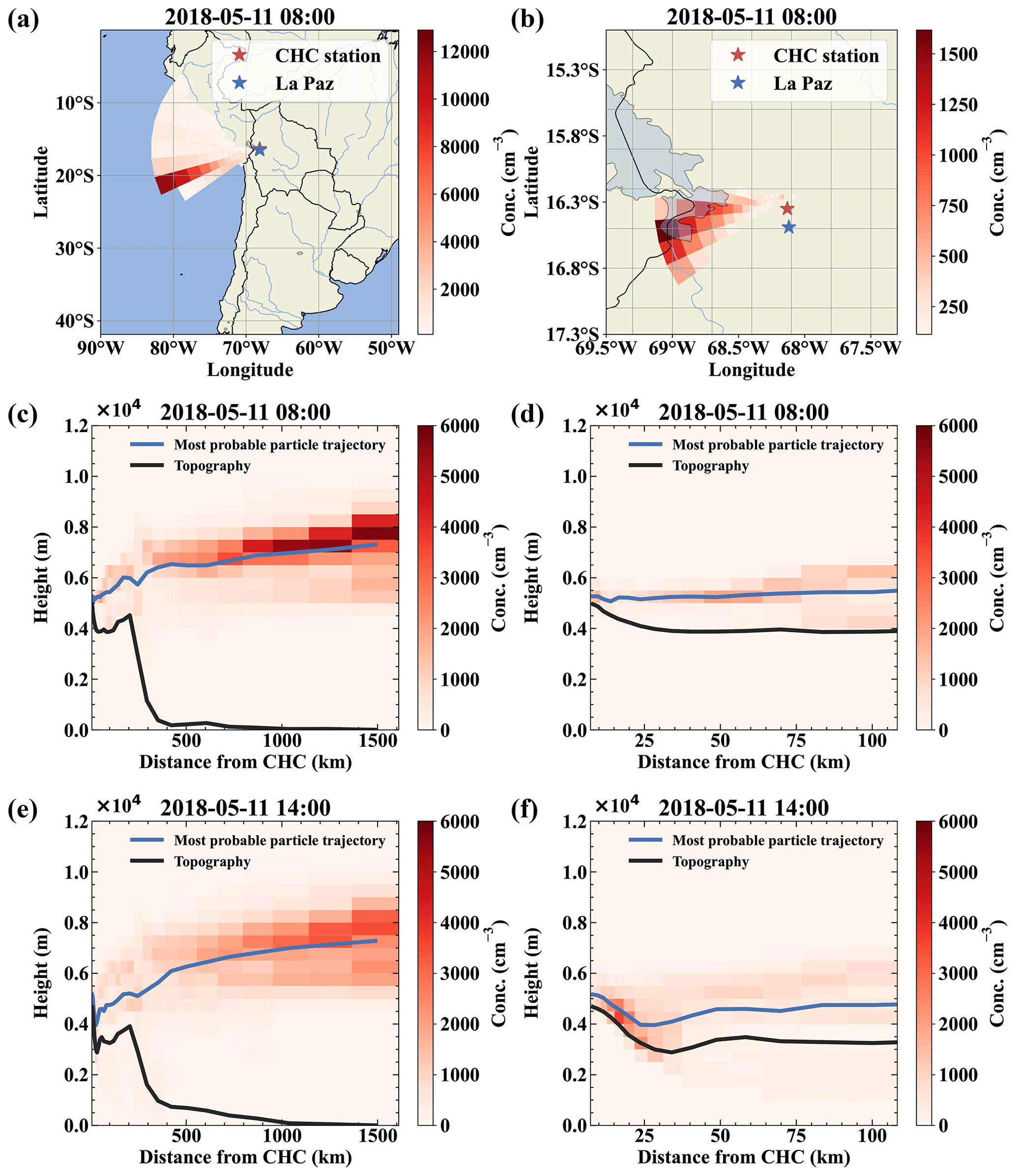
Figure 4Air mass origin comparison for a free tropospheric event (a–d) and one with surface contact with the air masses (e, f). Panels (a) and (b) show the top-down view of the most likely source regions (color-coded in red), showing the origin of the air parcels during the free tropospheric event on 11 May. Panels (c) and (d) show the same data but height resolved together with the topography as a vertical cut through the atmosphere in the direction of the most likely origin (west-southwest). For comparison, panels (e) and (f) show the most likely source of air parcels during a time with surface contact of the arriving air masses at 14:00 on the same day. Panels (b), (d), and (f) present a zoom on the local area close to Chacaltaya that mainly determines the influence of local sources like anthropogenic emissions from La Paz and El Alto.
To summarize, a shallow and strong inversion close to the ground likely did not allow the mixing of the different air masses during the marked times. This gives us the unique opportunity to characterize the free tropospheric air masses reaching the station from the westerly sector (as typical for the Altiplano dry season) with our array of state-of-the-art mass spectrometers. To avoid uncertainties caused by the FLEXPART time resolution and the potential daytime-dependent over- and underprediction of the boundary layer influence, we also determine when the station is in the free troposphere above the shallow boundary layer by applying the conditions from Table 2.
Table 2Identified threshold values to determine periods with free tropospheric (FT) air from higher altitudes reaching CHC undisturbed by mixing with the local boundary layer during the dry season.
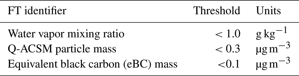
These FT identifiers are chosen after careful data analysis to be very strict so that we certainly exclude all periods affected by the boundary layer. We assume that all periods during which the conditions are not fulfilled are likely influenced by the local boundary layer to at least some extent, and we refer to them as BLday between 07:00 and 19:00 local time and BLnight otherwise. The FLEXPART analysis provides us with additional information on the horizontal and height-resolved transport of the air masses. Furthermore, the FLEXPART analysis can be considered a priori to data analysis, while the FT identifiers are set a posteriori and might vary with season (such as the water vapor mixing ratio).
Due to the limits of the FLEXPART domain, we cannot know exactly where the free tropospheric air masses had the last contact with the boundary layer, but chances are high that the last surface interaction occurred in a marine, remote setting over the south to the southwestern Pacific Ocean or in the intertropical convergence zone (ITCZ), as convection typically occurs in these areas, while it is typically unlikely in the southeastern Pacific due to the cold Humboldt upwelling. The enhanced gas-phase MSA concentrations during the marked undisturbed free tropospheric events, detected by the nitrate-CIMS and shown in Fig. 3a), are the first indication of this proposition. We also observed higher-than-median concentrations of MSA outside the marked periods, indicating that free tropospheric air masses mix in regularly. With our FT identification rule, we made sure to select events that are least impacted by surface emissions. That does not exclude the influence of FT air masses during other periods.
The Q-ACSM identifies the aerosols in the free troposphere as composed of sulfate and organics with only little ammonium and no nitrates (see also Fig. D2f in Appendix D1). The relative absence of nitrate observed in the particles by the Q-ACSM is reasonable, as it likely links to ammonium nitrate that forms from traffic emissions in the La Paz and El Alto metropolitan area and is thus solely emitted into the local boundary layer. The large sulfate fraction we observed probably has a regional origin and is not solely attributed to marine DMS oxidation, because CHC is influenced by volcanic emissions in the area (Bianchi et al., 2021), especially under westerly wind direction.
3.2 Ionic cluster composition in the free troposphere
The Positive-APi-TOF can give us information on the positive ion composition of the free tropospheric air masses. Using our previously gained understanding of the fingerprint of the FT events, we found an FT period under the westerly wind influence in February, when the instrument was operating.
In Fig. 5 we show a free tropospheric time period (19 February, 03:00–10:00) highlighted in green. A detailed air mass origin description for the FT event on 19 February is shown in Fig. E2 in Appendix E, which is close to the conditions of the event on 11 May.
Figure 5Time evolution of positive ions before, during, and after an FT event (green-shaded). (a) (NH3)DMSOH+, DMSOH+, and (H2O)DMSOH+ clusters, with arrows representing the wind direction on top. (b) Total positive ions (left axis), amines, and water ammonia clusters (right axis) from the Positive-APi-TOF. (c) Water vapor mixing ratio (left axis), radiation, temperature, and equivalent black carbon (eBC) (right axes).
As described above, the low water vapor mixing ratio (dropping from previously 4 to 0.8 g kg−1), low equivalent black carbon concentration (below 0.1 µg m−3), and low total number concentration of particles in the diameter range 10–650 nm (Fig. 5c) are indications of such FT events. The wind direction measured at the peak of the Chacaltaya mountain is shown as barbs in Fig. 5a, together with the time series of different DMSO clusters. DMSO has a proton affinity of 884.4 kJ mol−1. The signals of the typically dominating amines (proton affinities above 900 kJ mol−1) in the Positive-APi-TOF are significantly smaller during FT than during BL times (see Fig. 5b), while other compounds (unidentified, likely organics) take most of the charge (see Fig. E1 in Appendix E).
The signals of DMSOH+ and (H2O)DMSOH+ show an increase during the free tropospheric air event. This does not necessarily imply a higher DMSO concentration in the free troposphere; after all, (NH3)DMSOH+ was regularly present throughout the whole period (17–21 February) with maxima during nighttime and minima during daytime. This does indicate, however, the general presence of DMSO and additionally the lower abundance of species with higher proton affinities in FT air, which do typically affect the ionization likelihood of species with lower proton affinities (Eisele and Tanner, 1990). Therefore, the strong signals of DMSOH+ and (H2O)DMSOH+ and the decreased signal of (NH3)DMSOH+ show that ammonia, amines, and pyridine are significantly less available during FT times. Even though the water vapor mixing ratio decreased during the FT event, the water concentration in the atmosphere always remains high in contrast to other trace gases, which explains the slight increase of water clusters.
Comparing Fig. 5a and b shows that the signals of DMSO clusters are small compared to the total ions. The total ion counts remain high during the FT event, because the total ion concentrations in the atmosphere are determined by solar radiation, altitude, and other parameters. In our case, the ions switch from the species with the highest proton affinity to ones with lower proton affinity during air mass transition, which can explain the increase of the signal of unidentified organics, as shown in Fig. E1, and proves a significantly lower availability of high proton affinity compounds such as amines.
3.3 Observations of DMS oxidation products in the free troposphere
The molecular formulae of the organosulfur compounds detected in the gas phase by the PTR3 and nitrate-CIMS indicate that they are, in fact, oxidation products of DMS. In particular, we detected all presently known DMS oxidation products, except the recently observed HPMTF (Wu et al., 2015; Berndt et al., 2019; Veres et al., 2020), which might be below the detection limit.
We show their time series in Fig. D1 in Appendix D and present boxplots of the detected concentrations in the different air masses in Fig. 6. DMS (Fig. 6a) and gas-phase MSA (Fig. 6g) show significantly enhanced concentrations in the free troposphere. MSA is in fact one of the few condensible vapors which are higher in FT air than during BLday and dominates the nitrate-CIMS' FT – BLday spectrum shown in Fig. D3 (Appendix D1). When comparing with Fig. D1, the sporadic high concentrations of DMS occur during the first analyzed FT air period on 11 May. One rare subtropical storm, which was observed from 4 to 9 May only a few hundred kilometers off the Chilean coast (NESDIS, 2018), might have impacted our data and could explain the surprisingly high DMS concentration in such a large distance from the typically convective regions over the southern Pacific substantially further west.
Figure 6Boxplots of gas-phase DMS oxidation products, detected by the PTR3 and nitrate-CIMS in the FT (free troposphere without boundary layer influence), BLnight (within boundary layer during nighttime) and BLday (within boundary layer during daytime) air masses, respectively. The plots are based on 32 data points from averaged 30 min intervals each, with nighttime and daytime boundary layer conditions chosen to be as close in time as possible to FT periods with the same prevailing wind direction (horizontal air mass origin) for optimal comparison. The orange line shows the median, and the green triangle shows the mean value of the data.
Gas-phase H2SO4 (Fig. 6h) is strongly enhanced in the FT compared to the BLnight but is maximal in BLday. Since H2SO4 formation is driven by photochemistry, a diurnal maximum in the H2SO4 concentration can be explained, if local production, e.g., from SO2 oxidation occurs, although enhanced losses onto particles during BLday (Fig. D2d in Appendix D1) have a decreasing effect on the H2SO4 gas-phase concentration. Due to the influence of the metropolitan area of La Paz and El Alto and volcanic emissions, we expect H2SO4 to have a large OH-initiated production rate by oxidation of anthropogenic and volcanic SO2 during daytime. The high concentration of H2SO4 in the FT is partly explained by an increase in sulfuric acid directly after sunrise as some of the FT periods extended into the morning hours. Additionally, the lower condensation sink during the FT periods enhances the sulfuric acid lifetime during these events. This is especially evident in the night of 20 May: although in the middle of the night, where we expect the production term to be small, a substantial amount of sulfuric acid is observed that behaves anticorrelated to the low condensation sink during the event, as shown in Fig. D5 in Appendix D2.
The other oxidation products show a significantly weaker trend – but none shows features of a typical boundary layer product (compare to Fig. D2). However, as seen in Fig. 3, there is always an influence of free tropospheric air. A compound with little to no trend between those conditions could thus still have its origin in the free troposphere, but in such cases, additional local sources cannot be excluded and should be checked. We do this for MSIA (Fig. 6d) in Sect. 3.5. Afterwards, we relate their detected concentrations in Sect. 3.6.
3.4 Methanesulfonate and sulfate
The gas-phase MSA concentration in the FT is an order of magnitude higher than in the BL air (Fig. 6g), but, because of the low vapor pressure of MSA, we expect it to reach CHC mainly in the particle phase. We show the signal of particulate methanesulfonate (MSA), measured by the I−-FIGAERO-CIMS in Fig. 7a above the time series of the influence of the different air masses according to FLEXPART in Fig. 7b.
Figure 7MSA from the particle phase, evaporated and detected by the I−-FIGAERO-CIMS (a) and FLEXPART analysis of the relative influence of the different air masses (b). A strong increase of the methanesulfonate fraction within the particles is observed when the influence of free tropospheric long-range transport increases.
First of all, the FLEXPART analysis shows that the station is under the influence of free tropospheric air throughout the described measurement period. The total (mainly organic) signal of the particle phase detected by the I−-FIGAERO-CIMS (gray in Fig. 7) shows strong spikes corresponding to the daily influence of the boundary layer at the station. In contrast to the total signal, the methanesulfonate (light blue) stays relatively constant throughout the week, and its fraction in the particles (dark blue, circles) is anticorrelated to the boundary layer influence (25–28 May). From 29 May onwards, we observed a higher fraction of the methanesulfonate signal, likely due to the increased fraction of air masses from outside the domain. Wind velocities are significantly higher in higher altitudes in the free troposphere, so air masses get transported over large distances. On the night of 30 May, the fraction of air parcels from the free troposphere reaches nearly 90 %. This includes the fraction of air parcels from outside the domain that reached up to even 40 % during this period. At this time, the methanesulfonate fraction in the particles also reached its maximum. This strongly suggests that the methanesulfonate reaches CHC via transport in the free troposphere and that there is no significant local source.
As the absolute methanesulfonate signal appears independent of the surface influence, we can also use sampling filter measurements with a very coarse time resolution. While the filter measurements do not allow a differentiation between the free troposphere and boundary layer air masses, they allow for investigating the methanesulfonate more quantitatively.
Figure 8Yearly pattern of methanesulfonate mass concentration in PM2.5 and PM10 particles, based on data between 2012 and 2017, taken at CHC (a) and westerly wind (SSW to NW) frequency as measured on the Chacaltaya mountaintop (b). In the months from December to March the wind is often coming from the east due to the Bolivian high (Bianchi et al., 2021). In these months methanesulfonate mass concentrations in the particles are significantly lower than during the rest of the year.
The long-term particle composition measurements using sampling filters cover the years 2012–2017 (Fig. 8a) and show that approximately 4±1 ng m−3 methanesulfonate is found in the particles from April to November, which corresponds to the time when westerly wind conditions occur regularly (Fig. 8b). The particulate mass concentration of methanesulfonate corresponds to an average number of roughly 2.5×10⁷ molecules cm−3, which is 1–2 orders of magnitude higher than the detected gas-phase methanesulfonic acid concentrations, in line with its low vapor pressure.
The strongly FT-dependent gas-phase MSA signal observed from the nitrate-CIMS (compared to the nearly constant methanesulfonate signal from the I−-FIGAERO-CIMS) could be explained in two ways: firstly, MSA is known to participate in new particle formation and growth to larger aerosol particles (Bates et al., 1992b; Ayers et al., 1996; Covert et al., 1992; Beck et al., 2021), and the condensation sink in surface-affected air masses is much higher compared to within free tropospheric air masses. In FT air, the mild condensation sink leads to a longer lifetime for gas-phase MSA, which can explain the higher concentration of gas-phase MSA in the periods of undisturbed free tropospheric air reaching CHC. Upon mixing of the free tropospheric air masses with the boundary layer, the stronger condensational loss of MSA to the aerosols fully scavenges the gas-phase MSA. Secondly, it has been suggested in earlier publications (Mauldin III et al., 1999; Zhang et al., 2014) that MSA might degas from methanesulfonate aerosol in air masses with low relative humidity. The herein analyzed FT events always involved very low relative humidities, so this effect might occur as well. Zhang et al. (2014) stated that parallel measurements of both MSA and DMSO are necessary to prove or disprove their MSA evaporation hypothesis. We relate MSA to the other oxidation products in Sect. 3.6 after considering the impact of local sources.
Local sources certainly impact H2SO4, as already discussed in Sect. 3.3. This is confirmed by comparing methanesulfonate and sulfate concentrations: sulfate fractions of 50 % were detected by the Q-ACSM (Fig. D2 in Appendix D1) even during the marked free troposphere periods, which means that approximately 100 ng m−3 of non-refractory PM1 would be made up of sulfate (see Fig. D2e and f).
In comparison, methanesulfonate from the filter measurements is only about 4 ng m−3 in May in PM2.5 and PM10 (Fig. 8a). The ratio between methanesulfonate and sulfate is thus below 0.04, which is significantly lower than in remote marine areas (Ayers et al., 1996), laboratory experiments (Shen et al., 2022), or at similarly cold temperatures in free tropospheric measurements of marine air (Froyd et al., 2009). This suggests that the remote marine particle composition is altered due to the volcanic SO2 emissions in higher altitudes prior to reaching CHC as mentioned in Bianchi et al. (2021). While we might be able to limit the impact of the anthropogenic emissions on our dataset by using the FT indicators discussed in Sect. 3.1, we are hesitant to exclude the volcanic impact on sulfuric acid and sulfate data even in the undisturbed FT periods (defined by the specifications in Table 2) due to the higher emission altitude of volcanoes. Therefore, our dataset does not allow any conclusions for the production of H2SO4 by DMS oxidation.
3.5 The impact of local sources and long-range transport on the time series of DMS oxidation products
To understand which sources impact the DMS oxidation products' time series measured at CHC, we show the source regions (“footprints”) of MSIA on a map together with the height-resolved domain lateral boundaries outside the white ring (see Sect. 2.4.1 for an explanation), determined from FLEXPART Lagrangian dispersion calculations, as an example.
It is important to note that this analysis is based on the full MSIA time series – not distinguishing between the free troposphere and the boundary layer. It shows source regions on the surface (inside the white ring) from which air masses likely traveled close to the surface and height-resolved source regions at the lateral boundaries (outside the white ring). We chose to show the footprint analysis of MSIA for multiple reasons: first, we wanted to show a compound with a short atmospheric lifetime on the order of a few hours, which gives more weight to local sources compared to distant ones, thus giving an upper limit for the influence of local sources. Second, the time series had to be above the limit of detection for most of the time to have as many valid data points as possible, which unfortunately excluded DMS. Finally, the PTR3's sensitivity to MSIA is at the kinetic limit, thus its time series is independent of humidity changes.
One of the resolved local source regions affecting the MSIA time series is the southern part of Lake Titicaca, which also shows enhanced chlorophyll concentrations in May 2018, as shown in Fig. 9. More details on Lake Titicaca are given in Sect. 2.1. The DMS flux from Lake Titicaca has not been determined so far, but DMS fluxes from other lakes are roughly 10 times lower than the average marine flux of DMS (Steinke et al., 2018; Ginzburg et al., 1998; Sharma et al., 1999).
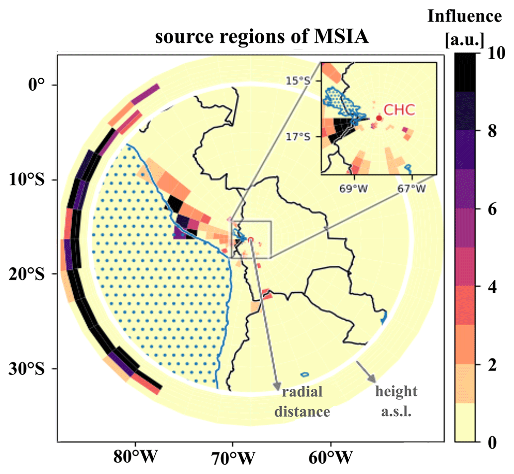
Figure 9FLEXPART source regions determined using the MSIA time series, showing a strong impact of transport through the FLEXPART domain lateral boundaries.
Compared to Lake Titicaca, the coast of Peru is a more important MSIA source according to the FLEXPART analysis – also showing enhanced chlorophyll concentrations in satellite images (see Fig. 9). Convection is very unlikely to occur at this cold and typically overcast coast of Peru in May, but the air masses might still move upslope thermally driven, thereby staying close to the mountain slope surface.
However, the FLEXPART backward dispersion analysis locates the major fraction of the MSIA source regions in the domain at the lateral boundaries in heights between 6000–8000 m a.s.l., suggesting that the air masses that carry DMS and DMS oxidation products are advected into the domain from the west (southwest to the northwest) and thus originate from the (remote) Pacific. For the other DMS oxidation products, the signal fraction explained by long-range advection is larger than for MSIA, as summarized in Table 3.
Table 3Relative influence of short-range transport of local emissions (SR, <100 km), long-range transport within the FLEXPART domain (LR, >100 km), and from sources outside of the domain (ooD, influx through lateral boundaries, >1600 km, free tropospheric transport).
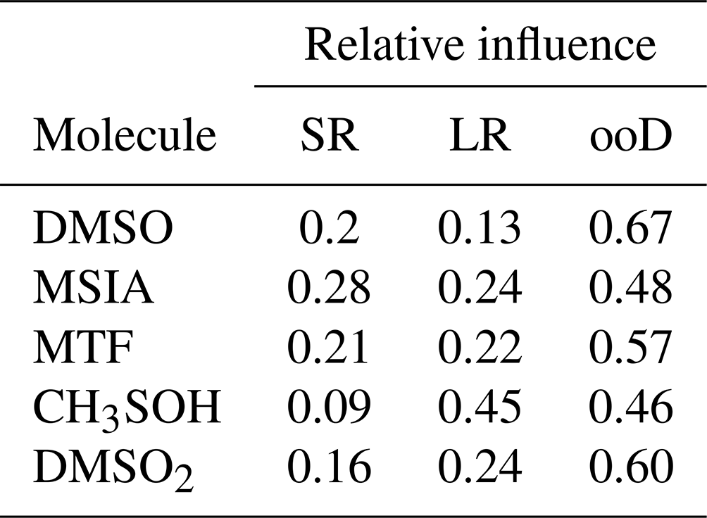
The differences in the allocation of source regions by FLEXPART for the various oxidation products likely originate from the different chemical transformation processes, which the Lagrangian dispersion model neglects. Despite the associated uncertainty, however, one result of the FLEXPART analysis is clear: local sources contribute around 20 % to the full time series of DMS oxidation products, while most of the signal is attributed to long-range transport with the largest fraction from outside of the domain. We can imply for our case – having even only a small impact of Lake Titicaca on the total time series – that the concentrations of DMS oxidation products measured in the FT air masses are a result of marine DMS emissions, long-range transport, and oxidation along the trajectory.
However, as described by Achá et al. (2018), the algal blooms in Lake Titicaca are likely to become more frequent in the future. Increasing DMS fluxes from Lake Titicaca would probably enhance especially the concentrations of DMS and its intermediates at CHC when the station is within the boundary layer.
3.6 Relating concentrations of DMS and its oxidation products with each other and to long-range transport
The observed DMS concentrations in comparison with the concentrations of its reaction products relate to a long reaction time during the transport from the source regions to Chacaltaya: the DMS signal is very variable, ranging from below detection limit (3×105 cm−3) to maximally 1×108 cm−3. We observed its highest concentration during the FT event on the morning of 11 May 2018. During this time, the air mass was coming from the west with high wind speeds. In fact, the air masses only require about 30 h to travel from the 1600 km distant lateral boundary of the simulated domain to CHC. This period is similar to the DMS lifetime of ca. 1.5 d in the atmosphere with respect to its main oxidant OH under halogen- and NOx-free conditions (Chen et al., 2018). Typical DMS concentrations in 6000–8000 m a.s.l. over the ocean are on the order of cm−3 (Thornton et al., 1992) but can reach up to 4×108 cm−3 close to convectional updrafts (Thornton and Bandy, 1993; Thornton et al., 1992). Consequently, the maximum value measured here is plausible if transport from a convective cell to CHC was on the order of the DMS lifetime. Interestingly, an extremely rare subtropical cyclone has been observed in the southeastern Pacific Ocean, only hundreds of kilometers away from the Chilean coast shortly before (9 May) (NESDIS, 2018), which most likely impacted the DMS concentrations at CHC. During all other FT events, the DMS concentration was cm−3 so that the major part of the DMS was already oxidized due to long transport times compared to the DMS lifetime.
All observed oxidation products except DMSO2 show gas-phase concentrations typically between molecules cm−3. DMSO2 is the only compound with gas-phase concentrations regularly in the 107−108 molecules cm−3 range. At air temperatures of approximately −10 ∘C at 6000 m a.s.l. (assuming a dry adiabatic temperature decrease with altitude above the Altiplano), DMSO2 is volatile to semivolatile (see Appendix A). In the free tropospheric air masses, DMSO2 will be far more abundant in the gas phase than in the particle phase. The measured mean gas-phase DMSO2 concentration of approximately 2×107 cm−3 in the free troposphere equals a mass concentration of 3.1 ng m−3. This is comparable to the total MSA mass concentration when taking the particle-phase data from the filter measurements (see Fig. 8a) into account (Sect. 3.4). Due to the close molar masses of DMSO2 and MSA, this implies similar amounts of sulfur in these two chemical states.
Such high DMSO2 yields are in contrast to chemical models, where DMSO2 is simulated to be only a minor oxidation product of the DMS addition pathway (Hoffmann et al., 2020), due to previously reported low concentrations of DMSO2 in the marine boundary layer (Davis et al., 1998; Berresheim et al., 1998). However, the colder temperatures and the long reaction time with negligible losses likely favor its accumulation in the free troposphere. High gas-phase DMSO2 concentrations were observed in lab experiments and were attributed to the reaction of DMSO with O3 at interfaces and in the aqueous phase (Berndt and Richters, 2012; Enami et al., 2016; Ye et al., 2021; Shen et al., 2022). The persistently high DMSO2 concentrations compared to other DMS oxidation products observed at Chacaltaya might therefore also indicate oxidation at air–liquid interfaces of aerosols or cloud droplets.
All other oxidation products were significantly less abundant, which likely has to do with their shorter lifetimes: the DMSO-to-DMSO2 ratio is relatively low, approximately 0.1. This is because the DMSO lifetime is short, typically hours, although DMSO is the precursor of DMSO2 under low-NOx conditions. The ratio between MSIA and DMSO2 is 0.03. Both compounds are products of DMSO oxidation, but MSIA has a similarly short lifetime like DMSO, while DMSO2 is photochemically inert with a lifetime of weeks and therefore builds up with reaction time along the trajectory. MTF (might be underestimated to some extent due to fragmentation), formed via H abstraction and reaction with HO2 and OH, thus requires two-step oxidation and is an intermediate product. It has an at least 5 times higher concentration than MSIA. This is reasonable because MTF also has a longer lifetime than MSIA: its lifetime is on the order of 6–12 h due to its lower photolysis and reaction rates (by OH radicals), while it is around 3 h for MSIA. MSA is detected at the kinetic limit in the nitrate-CIMS. DMSO, DMSO2, and MSIA are detected at the kinetic limit in the PTR3 (see the collision-induced dissociation ramps of DMSO, DMSO2, and MSIA in the H3O+-CIMS in Shen et al., 2022) so that this discussion is not impacted by uncertain calibration factors.
Furthermore, we measured signals close to the detection limits of our instruments at the exact masses of CH3S(O)2OOH (in nitrate-CIMS) and CH3SOH (in the PTR3) that both have unknown reaction rate constants and unfortunately also uncertain sensitivities. According to Berndt et al. (2020), the latter reacts quickly with ozone.
From the SALTENA campaign at the GAW station Chacaltaya (CHC) in the Bolivian Andes, we extracted periods corresponding to the prevalent influence of westerly free tropospheric air from the Pacific region to study marine-related chemical species transported over long distances.
Substantial signals of dimethyl sulfide (DMS) oxidation products were observed from all deployed state-of-the-art mass spectrometric techniques measuring both gas (APi-TOF, nitrate-CIMS, PTR3) and particle phase (ACSM and I−-FIGAERO-CIMS). We observed DMS itself and its oxidation products, H2SO4, MSA, DMSO, DMSO2, MSIA, MTF, CH3S(O)2OOH, and CH3SOH, of which several are highly soluble, showing the presence of DMS oxidation in the free troposphere. The array of time-of-flight mass spectrometers using different ionization methods and the low limit of detection allowed for the quantification of DMS, dimethylsulfoxide (DMSO), dimethylsulfone (DMSO2), methanesulfinic acid (MSIA), methanesulfonic acid (MSA), and sulfuric acid in parallel.
We have used a Lagrangian backward dispersion model (FLEXPART) to determine the source region of the DMS oxidation products within a domain of a 1600 km radius, which identified influx through the lateral boundaries in the free troposphere above the Pacific Ocean as the major source, suggesting an impact of convective updrafts from outside the FLEXPART domain. The model domain mainly covers the cold ocean waters affected by the upwelling Humboldt current that favor thermal inversion. Therefore these areas do not appear as sources of DMS reaching the Chacaltaya station.
The free tropospheric ion composition showed a strong reduction of amines compared to that in boundary layer conditions, allowing DMSO to get protonated. DMSO2 was found to have the highest concentrations of all DMS oxidation products in the gas phase. Gas-phase MSA concentrations reached up to 2×106 cm−3 whenever the air masses exhibited especially low particle loads and water vapor mixing ratios, enhanced by a factor of 10 compared to the median MSA concentration. Nonetheless, even during periods with high condensation sink, we still found MSA in the particulate phase, around 3 ng m−3, which is comparable to the amount of DMSO2 in terms of DMS-derived sulfur reaching CHC. Gas-phase MSA is therefore a good tracer for times when long-range transport from the ocean and minimal influence from local surface emissions co-occur, while the long-term dataset of particulate MSA indicates that the station is regularly influenced by air masses with marine origin. The effect of DMS oxidation on particle composition is nonetheless small, as it is competing with other sources of H2SO4 like volcanic SO2 in the region. This made it impossible to relate the MSA to H2SO4 ratio to DMS oxidation conditions.
While previous measurements already suggested DMS oxidation in the free troposphere, such a full spectrum of compounds from DMS oxidation as presented here has not been observed previously at such altitude and distance from sources, which provides insights into the fate of DMS in the free troposphere. Clearly, due to dilution and (wet) deposition losses, the concentrations of DMS oxidation products detected this far away from their sources are small. Our data suggest that their concentrations are too small to have an impact on new particle formation or growth directly at CHC, but – as previous results from flight campaigns have shown – particle formation and growth likely occur along the way, while concentrations of MSA and DMS-derived sulfuric acid are still less diluted, and the air masses are not impacted by volcanic emissions. To properly quantify the impact of DMS oxidation in the free troposphere, laboratory studies on particle formation rates with varying MSA and sulfuric acid concentrations and flight campaigns closer to marine updrafts with modern low-detection-limit proton transfer and nitrate cluster reaction mass spectrometers are needed in combination with physical and chemical aerosol characterization.
Dimethylsulfone, DMSO2, is a solid under typical atmospheric conditions in its bulk form. Only from 382 K onwards its vapor pressure data are available so that we need to estimate it. Using the data for DMSO2 as obtained from the National Institute of Standards and Technology Web Thermo Tables (NIST WTT) at the lowest available temperature (https://wtt-pro.nist.gov/wtt-pro/ (last access: 12 January 2023), To=382 K, po=0.7384 kPa, ΔHvap=66 kJ mol−1), and
we find that g m µg m−3. The temperature dependence of the equilibrium gas-phase concentration is approximately
according to the Clausius–Clapeyron equation. With the DMSO2-specific constants from above, this gives approximately µg m−3, which classifies DMSO2 as a volatile to semivolatile compound (Donahue et al., 2011, 2012). It will therefore not contribute to particle formation but might partition into the liquid aerosol phase due to its high water solubility. This is independent of the droplet acidity according to De Bruyn et al. (1994).
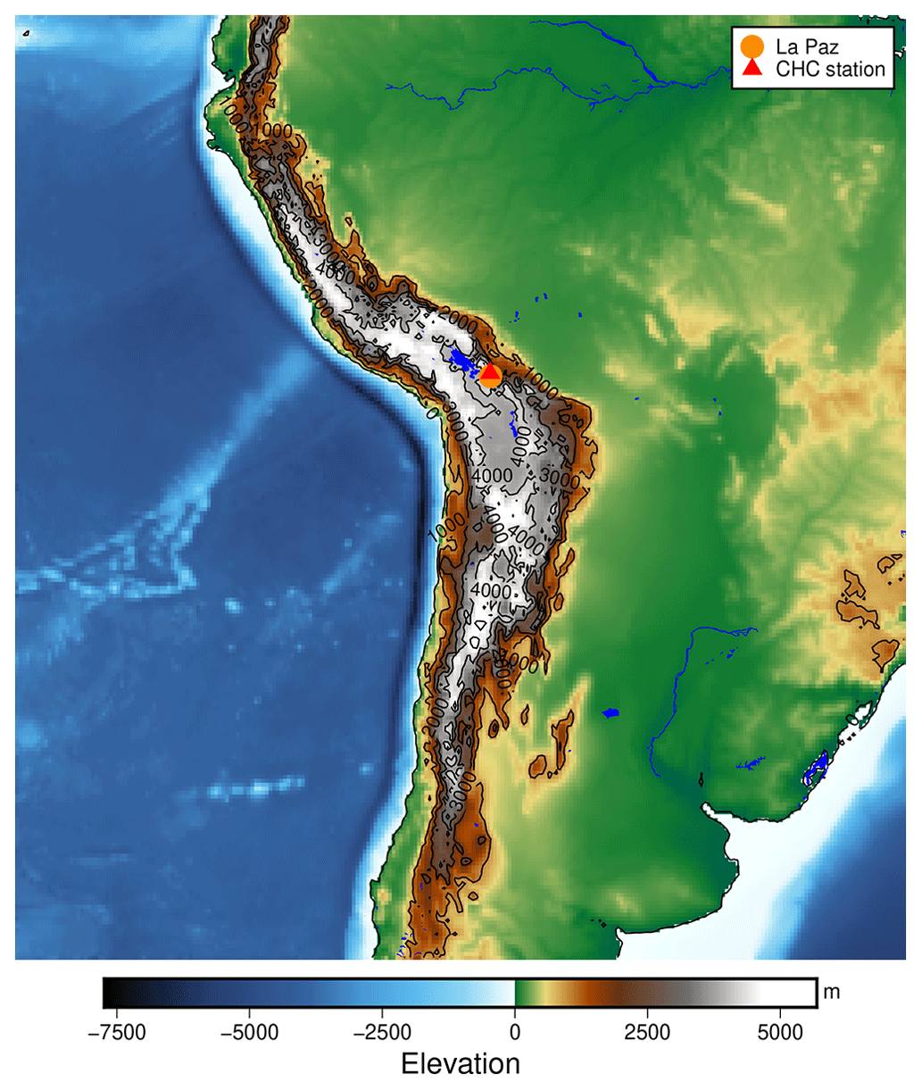
Figure B1The location of the Chacaltaya Global Atmosphere Watch (GAW) station in the Bolivian Andes. The elevation data shown are taken from Tozer et al. (2019).
Figure B1 gives a broad overview of the location of the measurements within South America. Located close to the ridge of the Andes, east of the Bolivian Altiplano at an altitude of 5200 m a.s.l., the station can be reached by free tropospheric air masses from the Pacific Ocean during the dry season and Amazon-influenced air masses during the wet season, as described in Bianchi et al. (2021).
C1 DMS calibration
The settings of the PTR3, described in Sect. 2.2.2, lead to a slightly humidity-dependent primary ion distribution, as shown in Fig. C1. No clusters larger than (H2O)2H3O+ are stable at the set value of 106±25 Td. Therefore, the sensitivity towards molecules that can be ionized efficiently by all of H3O+, (H2O)H3O+, and (H2O)2H3O+ does not exhibit a humidity dependence. Molecules like DMS have a humidity dependence and need to be calibrated, because their gas-phase basicity and proton affinity are not sufficient to get ionized by all of the clusters. The humidity-dependent sensitivity of DMS is shown together with that of acetonitrile in Fig. C2.
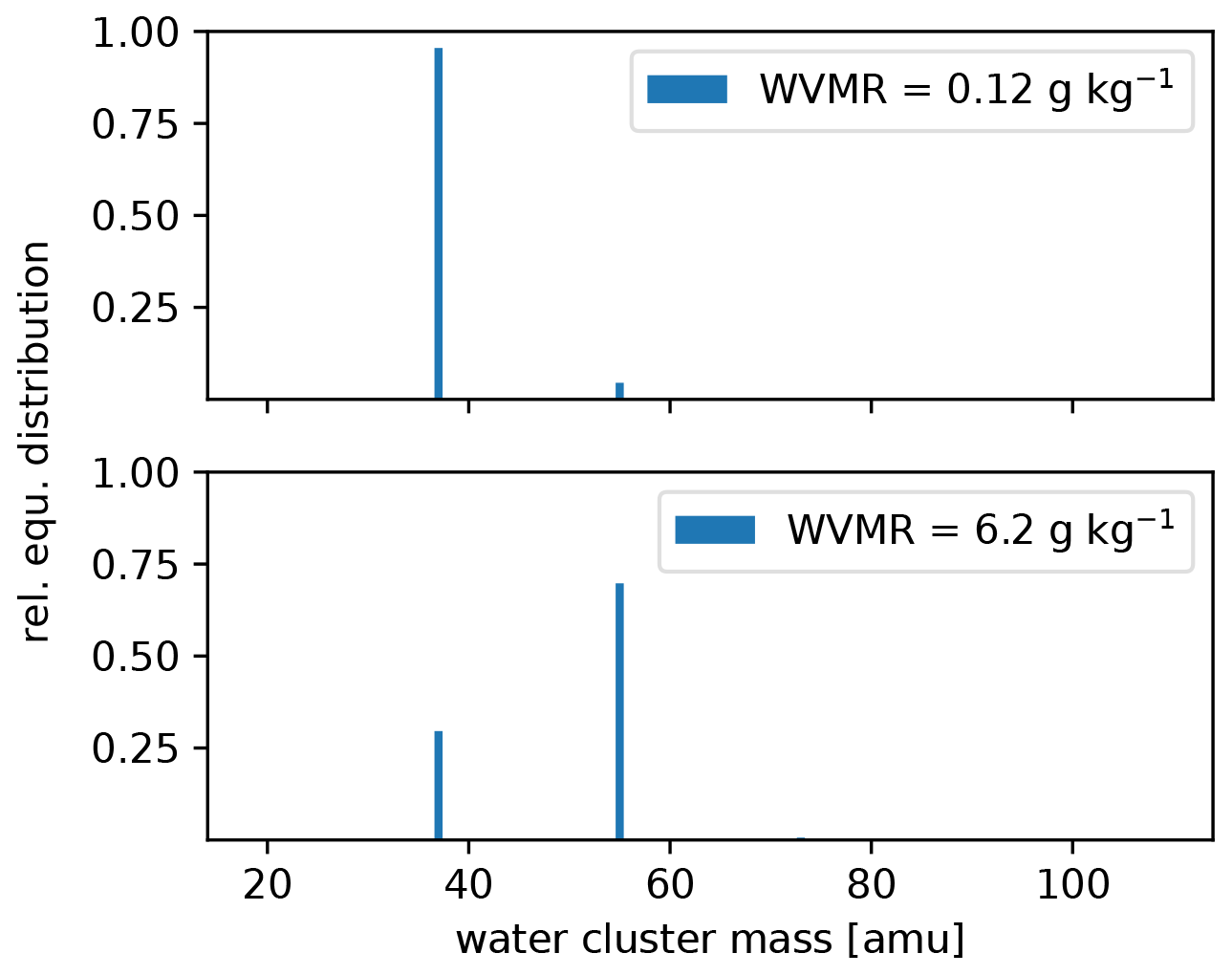
Figure C1Calculated equilibrium (equ.) primary ion distribution in the PTR3 at the minimum and maximum water vapor mixing ratio (WVMR) inside the PTR3 during the sampling period.
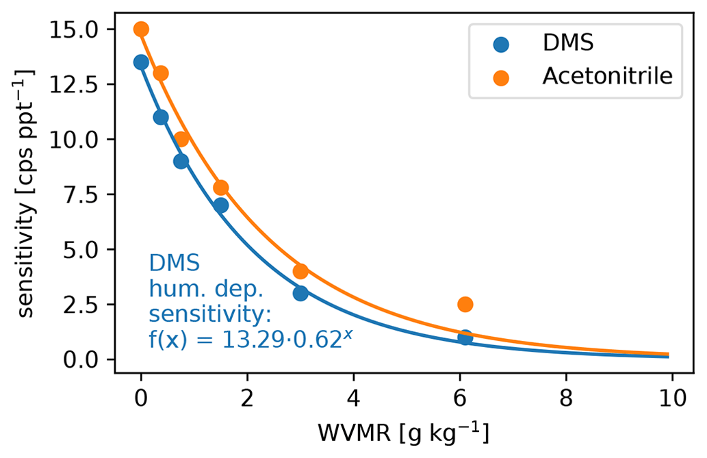
Figure C2Water vapor mixing ratio (WVMR) dependent calibration of DMS after the campaign together with the reference acetonitrile that we calibrated regularly during the campaign. The DMS calibration data points are fitted with an exponential decay function (shown) that we used to calibrate the DMS trace.

Figure C3Observed gas-phase organosulfur compounds from the PTR3 (blue) and nitrate-CIMS (orange) with their (lower-limit) concentration distributions (violins) and limit of detections (LODs, diamonds).
C2 Measured gas-phase concentration distributions compared to the detection limits of the DMS-related molecules in the PTR3 and nitrate-CIMS
As concentrations in the free troposphere are generally small, a careful test of the limit of detection above which concentrations are trustworthy needs to be performed. In a mass spectrum, each signal peak can have another limit of detection, as it also depends on the background signal on the exact mass of the compound of interest and its stability. This background can be caused by other molecules (or their isotopes) with a similar exact mass, which might show a different daily pattern. The limit of detection was thus estimated for each of the compounds of interest by taking into account any crosstalk of neighboring peaks in the mass spectrum.
In this Appendix, we have collected some figures that may help the interested reader to better understand the development process of our results and conclusions presented in the main section.
Figure D1 shows the time series of the gas-phase concentrations of the different observed molecules belonging to the DMS scheme, which are also available as a dataset under Scholz et al. (2022).

Figure D1Time series of all detected compounds (measured by the PTR3 and nitrate-CIMS) that belong to the DMS oxidation scheme during 2 weeks of May 2018.
D1 Comparison with boundary layer compounds
Figure D2 allows us to relate the FT and BL dependence of DMS and its oxidation products in Fig. 6 to the usual behavior of boundary-layer-affected measurands. Here we would also like to reiterate that nearly all of the gas-phase molecules observed in the mass spectra of the nitrate-CIMS and PTR3 clearly follow the pattern of boundary-layer-affected substances and that the signals within the boundary layer are typically orders of magnitude higher during the day than in the free troposphere, while this is not true for the DMS and its oxidation products. This is also evident in Fig. D3, which shows spectra of the nitrate-CIMS in the boundary layer (downward) and in the free troposphere (upward). The latter is clearly dominated by MSA.
D2 Nighttime sulfuric acid and the condensation sink
In Fig. 6 in Sect. 3.3 we have shown that the concentration of sulfuric acid in the free troposphere is high compared to the nighttime sulfuric acid in the boundary layer. While parts of the free tropospheric (FT) periods are after sunrise, we see in Fig. D5 that the sulfuric acid concentration is also high during nighttime FT periods, such as the night of 20 May. This is likely connected to the low condensation sink that we show together with the sulfuric acid in the same figure.
To calculate the condensation sink, we followed the approach described in Leskinen et al. (2008) with mean free path, diffusion coefficient, and size-resolved particle number concentration at 500 mbar pressure. Because the diffusivity is antiproportional and the number concentration proportional to the pressure, they cancel each other out, and we can use the diffusivity and the number size distribution both given at 1013 mbar standard pressure. For the diffusivity we used m2 s−1, the mean literature value for sulfuric acid, extracted from the compilation by Brus et al. (2016) for 278 K. The mean free path has to be pressure-corrected; however, as it does not cancel out. For 500 mbar we used a mean free path of 138 nm.
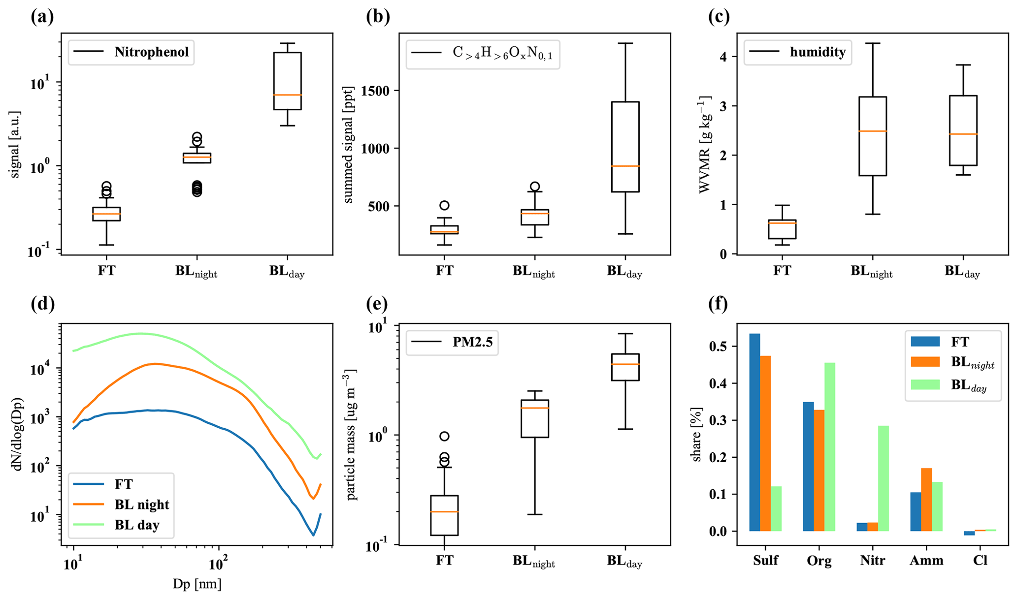
Figure D2The first row shows nitrophenol (a), total organics (b), and water vapor mixing ratio (c); the second row summarizes particle size distribution (d), total PM2.5 mass (e), and composition (f). The plots are based on 32 data points from averaged 30 min intervals each, with nighttime and daytime boundary layer conditions chosen to be as close in time as possible to FT periods with the same prevailing wind direction (horizontal air mass origin) for optimal comparison.
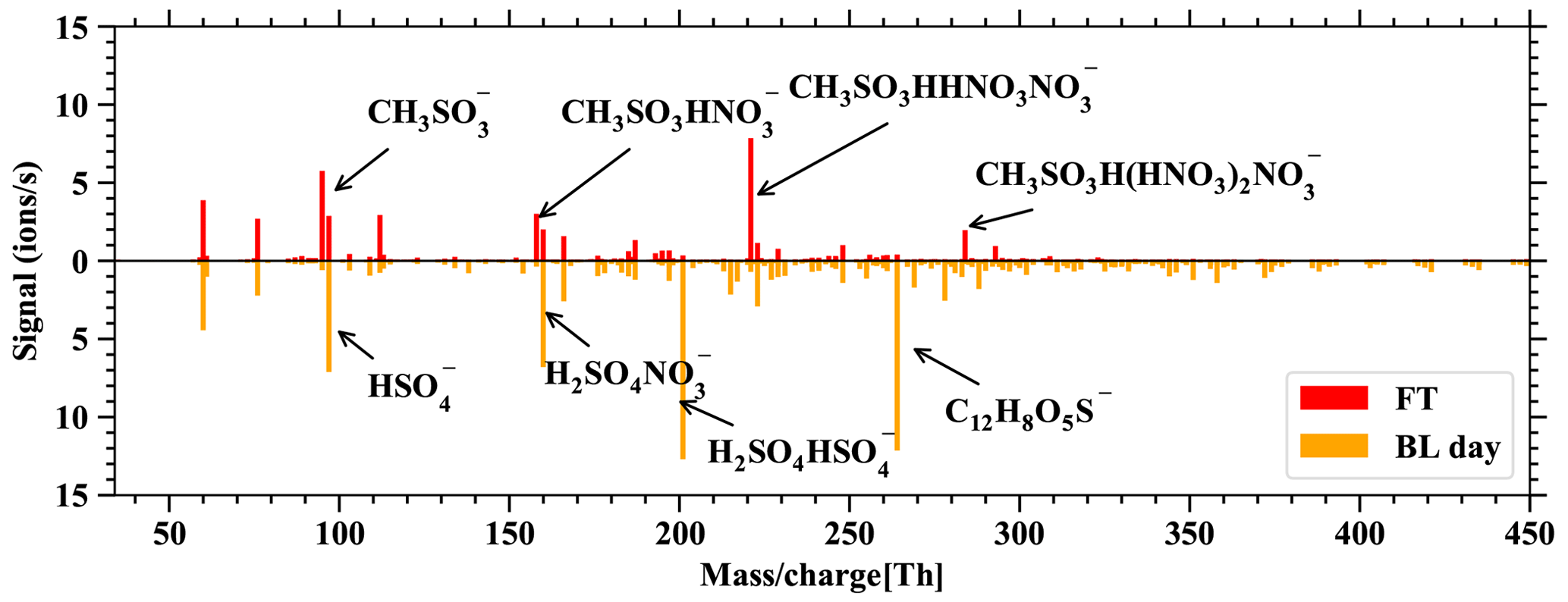
Figure D3Spectra of the nitrate-CIMS, showing the difference between FT – BLday on the positive axis and BLday – FT on the negative axis. Only very few compounds are larger in FT than BLday: the positive spectrum is dominated by clusters of the primary ions with MSA.
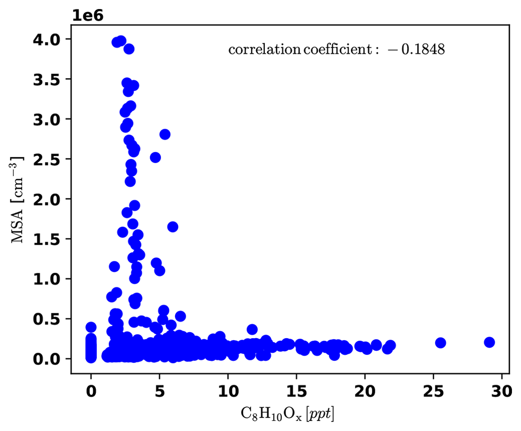
Figure D4Correlation plot of MSA and C8H10Ox, showing that MSA is high only when C8H10Ox is low and the other way round.
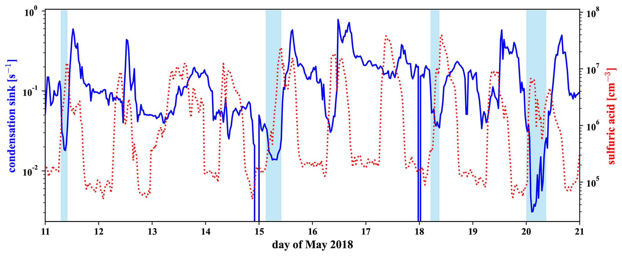
Figure D5Time series of sulfuric acid in red and of the condensation sink (pressure-corrected) in blue, calculated as described below. Marked in light blue are the identified FT periods.
Figure E1 shows additional information for the discussion in Sect. 3.2 where we presented the time evolution of positively charged DMSO clusters under different air masses. However, other positively charged compounds such as organics are not presented in the time series and are instead displayed in mass defect plots in Fig. E1, which focus on the difference in ion composition between the boundary layer and free troposphere by extracting the periods corresponding to the prevalent influence.
The nighttime ion spectrum in the boundary layer (Fig. E1a) is dominated by amine groups (colored circles), including alkyl propyl amines ((CH3)3(CH2)nNH+), alkyl pyrroline (C4H7(CH2)nNH+), alkyl pyridines (C5H5(CH2)nNH+), alkyl pyrrolidine (C4H10(CH2)nNH+), alkyl didehydropyridine (C5H4(CH2)nNH+), alkyl indole (C8H7(CH2)nNH+), alkyl benzazocine (C11H9(CH2)nNH+), alkyl quinoline (C9H7(CH2)nNH+), etc. Besides the amines, charged water clusters and water ammonia clusters are the second major species. This is likely due to their abundant concentration in the boundary layer, although water and ammonia have lower proton affinity than the amines. The charged water and water ammonia clusters usually contain 6 to 11 water molecules according to the ion spectrum in Fig. E1. However, we are not able to observe all the clusters in the ion spectrum, because some of them interfere with the species that have similar mass-to-charge ratios. For example, is not visible due to C10H10N+, which has a stronger signal as shown in Fig. E1a.
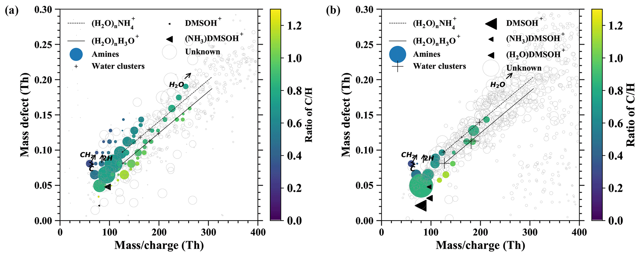
Figure E1The mass defect for airborne ions in the continental boundary layer (a) and the free troposphere (b). The data are averaged over 1 h.
The air mass origins shown in Fig. E2 help to confirm that our ionic dataset is comparable with the free tropospheric periods during the intensive measurement period in May.
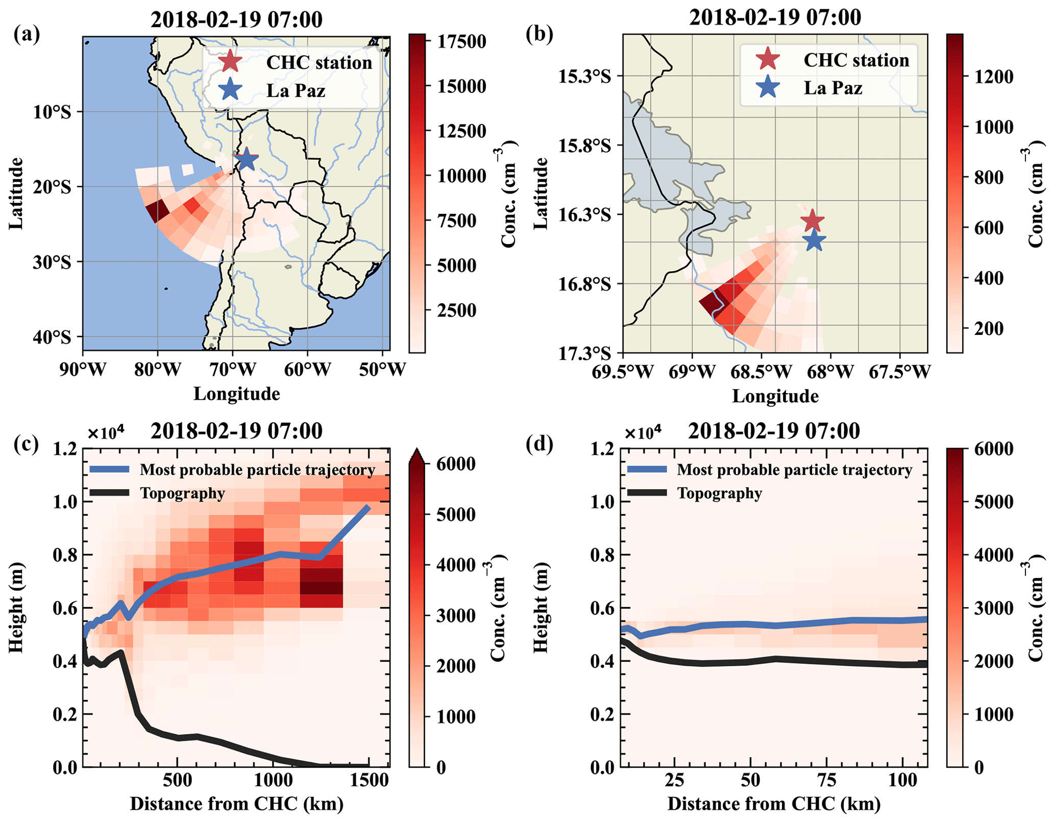
Figure E2Air mass origin of a free tropospheric event on 19 February. Panels (a) and (b) show the top-down view of the most likely source regions for the air parcels from west-southwest, which is close to the conditions on 11 May. Panels (c) and (d) show the same data but height resolved together with the topography as a vertical cut through the atmosphere.
The time series of the different presented variables and the python codes for plotting the figures can be found under https://doi.org/10.5281/zenodo.7429639 (Scholz et al., 2022).
WS, QZ and JS, CW, and SC, and PA analyzed the data of the mass spectrometers PTR3, nitrate-CIMS and APi-TOF, I−-FIGAERO-CIMS, and Q-ACSM, respectively. DA performed the FLEXPART Lagrangian dispersion simulations and analysis; JLJ analyzed the long-term aerosol filter samples with support from PG and GU; WS, DA, CW, SC, IM, QZ, WH, LH, JLJ, EP, ML, FV, CM, and FB collected the data and operated the instruments during the measurement campaign; and PL and MA cofounded the CHC GAW station and oversaw the atmospheric research at the station since the beginning. PG and GU provided organizational and financial support for the long-term research. PG also ensured custom clearance of all instruments involved in the SALTENA campaign. WS and JS wrote the manuscript with contributions from VS, contributed to data interpretation, and editing of the manuscript. All authors commented on the manuscript.
The contact author has declared that none of the authors has any competing interests.
Publisher's note: Copernicus Publications remains neutral with regard to jurisdictional claims in published maps and institutional affiliations.
We thank the Bolivian staff of the Institute for Physics Research, UMSA (IIF-UMSA), who work at CHC for their valuable work under difficult conditions and the Institute for Research and Development (IRD) personnel for the logistic and financial support during the campaign, including shipping and customs concerns. We also acknowledge the IT Center for Science (CSC), Finland, for generous computational resources that enabled the WRF and FLEXPART-WRF simulations to be conducted.
The long-term observations used in SALTENA are performed within the framework of GAW and ACTRIS, receiving support from the Universidad Mayor de San Andrés and from the international stakeholders. In France, support from the Centre national de la recherche scientifique through ACTRIS-FR/SNO CLAP and research infrastructure DATA TERRA, as well as the Institut de Recherche et Développement (IRD) and Observatoire des Sciences de l'Univers de Grenoble (OSUG) through the French National Research Agency's Laboratories of Ecellence in particular, is greatly acknowledged. All long-term measurements of the filter chemistry were performed on the Air O Sol analytical platform at IGE (Grenoble).
We acknowledge the use of imagery from the Aqua MODIS satellite, provided by services from NASA's Global Imagery Browse Services (GIBS), a part of NASA's Earth Observing System Data and Information System (EOSDIS). We thank all the funders who made this project possible with their financial support.
This research has been supported by the H2020 Marie Sklodowska-Curie Actions (project CLOUD-Motion, grant no. 76991) and the H2020 European Research Council (project CHAPAs, grant no. 850614, and ATM-GP, grant no. 742206). This research has also been supported by the Academy of Finland (via projects 311932, their flagship funding no. 337549, and their Center of Excellence, project no. 315203) and the Knut and Alice Wallenberg Foundation via the WAF project CLOUDFORM no. 2017.0165. Paolo Artaxo received funds from the Fundação de Amparo à Pesquisa do Estado de Sao Paulo (FAPESP, grant no. 2017/17047-0) and Wiebke Scholz was supported by the University of Innsbruck in the form of a doctoral scholarship (2021/01).
This paper was edited by Marc von Hobe and reviewed by two anonymous referees.
Achá, D., Guédron, S., Amouroux, D., Point, D., Lazzaro, X., Fernandez, P. E., and Sarret, G.: Algal bloom exacerbates hydrogen sulfide and methylmercury contamination in the emblematic high-altitude lake titicaca, Geosciences, 8, 438, https://doi.org/10.3390/geosciences8120438, 2018. a, b, c, d
Aliaga, D.: FLEXPART-WRF_v3.3.2 modified code, Zenodo [code], https://doi.org/10.5281/zenodo.5516295, 2021. a
Aliaga, D., Sinclair, V. A., Andrade, M., Artaxo, P., Carbone, S., Kadantsev, E., Laj, P., Wiedensohler, A., Krejci, R., and Bianchi, F.: Identifying source regions of air masses sampled at the tropical high-altitude site of Chacaltaya using WRF-FLEXPART and cluster analysis, Atmos. Chem. Phys., 21, 16453–16477, https://doi.org/10.5194/acp-21-16453-2021, 2021. a, b, c, d, e, f, g, h
Andreae, M. O.: The Production of Methylated Sulfur Compounds by Marine Phytoplankton, Springer Berlin Heidelberg, Berlin, Heidelberg, 253–259, https://doi.org/10.1007/978-3-662-26582-6_26, 1980. a
Ayers, G. P., Cainey, J. M., Granek, H., and Leck, C.: Dimethylsulfide oxidation and the ratio of methanesulfonate to non sea-salt sulfate in the marine aerosol, J. Atmos. Chem., 25, 307–325, https://doi.org/10.1007/bf00053798, 1996. a, b, c, d
Baccarini, A., Karlsson, L., Dommen, J., Duplessis, P., Vüllers, J., Brooks, I. M., Saiz-Lopez, A., Salter, M., Tjernström, M., Baltensperger, U., Zieger, P., and Schmale, J.: Frequent new particle formation over the high Arctic pack ice by enhanced iodine emissions, Nat. Commun., 11, 4924, https://doi.org/10.1038/s41467-020-18551-0, 2020. a
Bardouki, H., Berresheim, H., Vrekoussis, M., Sciare, J., Kouvarakis, G., Oikonomou, K., Schneider, J., and Mihalopoulos, N.: Gaseous (DMS, MSA, SO2, H2SO4 and DMSO) and particulate (sulfate and methanesulfonate) sulfur species over the northeastern coast of Crete, Atmos. Chem. Phys., 3, 1871–1886, https://doi.org/10.5194/acp-3-1871-2003, 2003. a
Barnes, I., Hjorth, J., and Mihalopoulos, N.: Dimethyl Sulfide and Dimethyl Sulfoxide and Their Oxidation in the Atmosphere, Chem. Rev., 106, 940–975, https://doi.org/10.1021/cr020529+, 2006. a, b
Bates, T., Lamb, B., Guenther, A., Dignon, J., and Stoiber, R.: Sulfur Emissions to the Atmosphere from Natural Sources, J. Atmos. Chem., 14, 315–337, https://doi.org/10.1007/BF00115242, 1992a. a, b
Bates, T. S., Calhoun, J. A., and Quinn, P. K.: Variations in the methanesulfonate to sulfate molar ratio in submicrometer marine aerosol particles over the south Pacific Ocean, J. Geophys. Res.-Atmos., 97, 9859–9865, https://doi.org/10.1029/92JD00411, 1992b. a
Beck, L. J., Sarnela, N., Junninen, H., Hoppe, C. J. M., Garmash, O., Bianchi, F., Riva, M., Rose, C., Peräkylä, O., Wimmer, D., Kausiala, O., Jokinen, T., Ahonen, L., Mikkilä, J., Hakala, J., He, X., Kontkanen, J., Wolf, K. K. E., Cappelletti, D., Mazzola, M., Traversi, R., Petroselli, C., Viola, A. P., Vitale, V., Lange, R., Massling, A., Nøjgaard, J. K., Krejci, R., Karlsson, L., Zieger, P., Jang, S., Lee, K., Vakkari, V., Lampilahti, J., Thakur, R. C., Leino, K., Kangasluoma, J., Duplissy, E., Siivola, E., Marbouti, M., Tham, Y. J., Saiz‐Lopez, A., Petäjä, T., Ehn, M., Worsnop, D. R., Skov, H., Kulmala, M., Kerminen, V., and Sipilä, M.: Differing mechanisms of new particle formation at two Arctic sites, Geophys. Res. Lett., 48, e2020GL091334, https://doi.org/10.1029/2020gl091334, 2021. a, b, c
Berndt, T. and Richters, S.: Products of the reaction of OH radicals with dimethyl sulphide in the absence of NOx: Experiment and simulation, Atmos. Environ., 47, 316–322, https://doi.org/10.1016/J.ATMOSENV.2011.10.060, 2012. a
Berndt, T., Scholz, W., Mentler, B., Fischer, L., Hoffmann, E. H., Tilgner, A., Hyttinen, N., Prisle, N. L., Hansel, A., and Herrmann, H.: Fast Peroxy Radical Isomerization and OH Recycling in the Reaction of OH Radicals with Dimethyl Sulfide, J. Phys. Chem. Lett., 10, 6478–6483, https://doi.org/10.1021/acs.jpclett.9b02567, 2019. a, b, c
Berndt, T., Chen, J., Møller, K. H., Hyttinen, N., Prisle, N. L., Tilgner, A., Hoffmann, E. H., Herrmann, H., and Kjaergaard, H. G.: SO2 formation and peroxy radical isomerization in the atmospheric reaction of OH radicals with dimethyl disulfide, Chem. Commun., 56, 13634–13637, https://doi.org/10.1039/D0CC05783E, 2020. a, b
Berresheim, H., Huey, J. W., Thorn, R. P., Eisele, F. L., Tanner, D. J., and Jefferson, A.: Measurements of dimethyl sulfide, dimethyl sulfoxide, dimethyl sulfone, and aerosol ions at Palmer Station, Antarctica, J. Geophys. Res.-Atmos., 103, 1629–1637, https://doi.org/10.1029/97JD00695, 1998. a, b
Berresheim, H., Elste, T., Tremmel, H. G., Allen, A. G., Hansson, H.-C., Rosman, K., Dal Maso, M., Mäkelä, J. M., Kulmala, M., and O'Dowd, C. D.: Gas-aerosol relationships of H2SO4, MSA, and OH: Observations in the coastal marine boundary layer at Mace Head, Ireland, J. Geophys. Res.-Atmos., 107, PAR 5–1–PAR 5–12, https://doi.org/10.1029/2000jd000229, 2002. a
Bianchi, F., Sinclair, V. A., Aliaga, D., Zha, Q., Scholz, W., Wu, C., Heikkinen, L., Modini, R., Partoll, E., Velarde, F., Moreno, I., Gramlich, Y., Huang, W., Leiminger, M., Enroth, J., Peräkylä, O., Marinoni, A., Xuemeng, C., Blacutt, L., Forno, R., Gutierrez, R., Ginot, P., Uzu, G., Facchini, M. C., Gilardoni, S., Gysel-Beer, M., Cai, R., Petäjä, T., Rinaldi, M., Saathoff, H., Sellegri, K., Worsnop, D., Artaxo, P., Hansel, A., Kulmala, M., Wiedensohler, A., Laj, P., Krejci, R., Carbone, S., Andrade, M., and Mohr, C.: The SALTENA experiment: Comprehensive observations of aerosol sources, formation and processes in the South American Andes, B. Am. Meteorol. Soc., 1, 1–46, https://doi.org/10.1175/BAMS-D-20-0187.1, 2021. a, b, c, d, e, f, g, h, i
Breitenlechner, M., Fischer, L., Hainer, M., Heinritzi, M., Curtius, J., and Hansel, A.: The PTR3: A novel Instrument for studying the lifecycle of reactive organic carbon in the Atmosphere, Anal. Chem., 89, 5824-−5831, https://doi.org/10.1021/acs.analchem.6b05110, 2017. a
Brus, D., Skrabalova, L., Herrmann, E., Olenius, T., Travnickova, T., and Merikanto, J.: Temperature-dependent diffusion coefficient of H2SO4 in air: laboratory measurements using laminar flow technique, Atmos. Chem. Phys. Discuss. [preprint], https://doi.org/10.5194/acp-2016-398, 2016. a
Cavalli, F., Viana, M., Yttri, K. E., Genberg, J., and Putaud, J.-P.: Toward a standardised thermal-optical protocol for measuring atmospheric organic and elemental carbon: the EUSAAR protocol, Atmos. Meas. Tech., 3, 79–89, https://doi.org/10.5194/amt-3-79-2010, 2010. a
Charlson, R. J., Lovelock, J. E., Andreae, M. O., and Warren, S. G.: Oceanic phytoplankton, atmospheric sulphur, cloud albedo and climate, Nature, 326, 655–661, https://doi.org/10.1038/326655a0, 1987. a
Chen, Q., Sherwen, T., Evans, M., and Alexander, B.: DMS oxidation and sulfur aerosol formation in the marine troposphere: a focus on reactive halogen and multiphase chemistry, Atmos. Chem. Phys., 18, 13617–13637, https://doi.org/10.5194/acp-18-13617-2018, 2018. a
Covert, D. S., Kapustin, V. N., Quinn, P. K., and Bates, T. S.: New particle formation in the marine boundary layer, J. Geophys. Res.-Atmos., 97, 20581–20589, https://doi.org/10.1029/92JD02074, 1992. a, b
Davis, D., Chen, G., Kasibhatla, P., Jefferson, A., Tanner, D., Eisele, F., Lenschow, D., Neff, W., and Berresheim, H.: DMS oxidation in the Antarctic marine boundary layer: Comparison of model simulations and held observations of DMS, DMSO, DMSO2, H2SO4(g), MSA(g), and MSA(p), J. Geophys. Res.-Atmos., 103, 1657–1678, https://doi.org/10.1029/97JD03452, 1998. a
De Bruyn, W. J., Shorter, J. A., Davidovits, P., Worsnop, D. R., Zahniser, M. S., and Kolb, C. E.: Uptake of gas phase sulfur species methanesulfonic acid, dimethylsulfoxide, and dimethyl sulfone by aqueous surfaces, J. Geophys. Res.-Atmos., 99, 16927–16932, https://doi.org/10.1029/94JD00684, 1994. a
Donahue, N. M., Epstein, S. A., Pandis, S. N., and Robinson, A. L.: A two-dimensional volatility basis set: 1. organic-aerosol mixing thermodynamics, Atmos. Chem. Phys., 11, 3303–3318, https://doi.org/10.5194/acp-11-3303-2011, 2011. a
Donahue, N. M., Kroll, J. H., Pandis, S. N., and Robinson, A. L.: A two-dimensional volatility basis set – Part 2: Diagnostics of organic-aerosol evolution, Atmos. Chem. Phys., 12, 615–634, https://doi.org/10.5194/acp-12-615-2012, 2012. a
Dunne, E. M., Gordon, H., Kurten, A., Almeida, J., Duplissy, J., Williamson, C., Ortega, I. K., Pringle, K. J., Adamov, A., Baltensperger, U., Barmet, P., Benduhn, F., Bianchi, F., Breitenlechner, M., Clarke, A., Curtius, J., Dommen, J., Donahue, N. M., Ehrhart, S., Flagan, R. C., Franchin, A., Guida, R., Hakala, J., Hansel, A., Heinritzi, M., Jokinen, T., Kangasluoma, J., Kirkby, J., Kulmala, M., Kupc, A., Lawler, M. J., Lehtipalo, K., Makhmutov, V., Mann, G., Mathot, S., Merikanto, J., Miettinen, P., Nenes, A., Onnela, A., Rap, A., Reddington, C. L. S., Riccobono, F., Richards, N. A. D., Rissanen, M. P., Rondo, L., Sarnela, N., Schobesberger, S., Sengupta, K., Simon, M., Sipila, M., Smith, J. N., Stozkhov, Y., Tome, A., Trostl, J., Wagner, P. E., Wimmer, D., Winkler, P. M., Worsnop, D. R., and Carslaw, K. S.: Global atmospheric particle formation from CERN CLOUD measurements, Science, 354, 1119–1124, https://doi.org/10.1126/science.aaf2649, 2016. a
Duquesne, F., Vallaeys, V., Vidaurre, P. J., and Hanert, E.: A coupled ecohydrodynamic model to predict algal blooms in Lake Titicaca, Ecol. Model., 440, 109418, https://doi.org/10.1016/j.ecolmodel.2020.109418, 2021. a
Edtbauer, A., Stönner, C., Pfannerstill, E. Y., Berasategui, M., Walter, D., Crowley, J. N., Lelieveld, J., and Williams, J.: A new marine biogenic emission: methane sulfonamide (MSAM), dimethyl sulfide (DMS), and dimethyl sulfone (DMSO2) measured in air over the Arabian Sea, Atmos. Chem. Phys., 20, 6081–6094, https://doi.org/10.5194/acp-20-6081-2020, 2020. a
Eisele, F. L. and Tanner, D. J.: Identifications of ions in continental air, J. Geophys. Res. 95, 20539–20550, https://doi.org/10.1029/JD095iD12p20539, 1990. a
Enami, S., Sakamoto, Y., Hara, K., Osada, K., Hoffmann, M. R., and Colussi, A. J.: Heterogeneous Chemistry in the Conversion of Gaseous Dimethyl Sulfide to Atmospheric Particles, Environ. Sci. Technol., 50, 1834–1843, https://doi.org/10.1021/acs.est.5b05337, 2016. a
Franklin, D. J., Steinke, M., Young, J., Probert, I., and Malin, G.: Dimethylsulphoniopropionate (DMSP), DMSP-lyase activity (DLA) and dimethylsulphide (DMS) in 10 species of coccolithophore, Mar. Ecol. Prog. Ser., 410, 13–23, https://doi.org/10.3354/MEPS08596, 2010. a
Froyd, K. D., Murphy, D. M., Sanford, T. J., Thomson, D. S., Wilson, J. C., Pfister, L., and Lait, L.: Aerosol composition of the tropical upper troposphere, Atmos. Chem. Phys., 9, 4363–4385, https://doi.org/10.5194/acp-9-4363-2009, 2009. a, b
Ginzburg, B., Chalifa, I., Gun, J., Dor, I., Hadas, O., and Lev, O.: DMS formation by dimethylsulfoniopropionate route in freshwater, Environ. Sci. Technol., 32, 2130–2136, https://doi.org/10.1021/ES9709076, 1998. a
Gordon, H., Kirkby, J., Baltensperger, U., Bianchi, F., Breitenlechner, M., Curtius, J., Dias, A., Dommen, J., Donahue, N. M., Dunne, E. M., Duplissy, J., Ehrhart, S., Flagan, R. C., Frege, C., Fuchs, C., Hansel, A., Hoyle, C. R., Kulmala, M., Kürten, A., Lehtipalo, K., Makhmutov, V., Molteni, U., Rissanen, M. P., Stozkhov, Y., Tröstl, J., Tsagkogeorgas, G., Wagner, R., Williamson, C., Wimmer, D., Winkler, P. M., Yan, C., Carslaw, K. S., and Gordon, A. L.: Journal of Geophysical Research: Atmospheres Causes and importance of new particle formation in the present-day and preindustrial atmospheres, Res. Atmos., 122, 8739–8760, https://doi.org/10.1002/2017JD026844, 2017. a
Hoffmann, E. H., Tilgner, A., Schrödner, R., Bräuer, P., Wolke, R., and Herrmann, H.: An advanced modeling study on the impacts and atmospheric implications of multiphase dimethyl sulfide chemistry, P. Natl. Acad. Sci. USA, 113, 11776–11781, https://doi.org/10.1073/pnas.1606320113, 2016. a
Hoffmann, E. H., Schrödner, R., Tilgner, A., Wolke, R., and Herrmann, H.: CAPRAM reduction towards an operational multiphase halogen and dimethyl sulfide chemistry treatment in the chemistry transport model COSMO-MUSCAT(5.04e), Geosci. Model Dev., 13, 2587–2609, https://doi.org/10.5194/gmd-13-2587-2020, 2020. a
Jokinen, T., Sipilä, M., Junninen, H., Ehn, M., Lönn, G., Hakala, J., Petäjä, T., Mauldin III, R. L., Kulmala, M., and Worsnop, D. R.: Atmospheric sulphuric acid and neutral cluster measurements using CI-APi-TOF, Atmos. Chem. Phys., 12, 4117–4125, https://doi.org/10.5194/acp-12-4117-2012, 2012. a
Junninen, H., Ehn, M., Petäjä, T., Luosujärvi, L., Kotiaho, T., Kostiainen, R., Rohner, U., Gonin, M., Fuhrer, K., Kulmala, M., and Worsnop, D. R.: A high-resolution mass spectrometer to measure atmospheric ion composition, Atmos. Meas. Tech., 3, 1039–1053, https://doi.org/10.5194/amt-3-1039-2010, 2010. a
Kürten, A., Rondo, L., Ehrhart, S., and Curtius, J.: Performance of a corona ion source for measurement of sulfuric acid by chemical ionization mass spectrometry, Atmos. Meas. Tech., 4, 437–443, https://doi.org/10.5194/amt-4-437-2011, 2011. a
Kürten, A., Rondo, L., Ehrhart, S., and Curtius, J.: Calibration of a chemical ionization mass spectrometer for the measurement of gaseous sulfuric acid, J. Phys. Chem. A, 116, 6375–6386, https://doi.org/10.1021/jp212123n, 2012. a
Lana, A., Bell, T. G., Simó, R., Vallina, S. M., Ballabrera-Poy, J., Kettle, A. J., Dachs, J., Bopp, L., Saltzman, E. S., Stefels, J., Johnson, J. E., and Liss, P. S.: An updated climatology of surface dimethlysulfide concentrations and emission fluxes in the global ocean, Global Biogeochem. Cy., 25, GB1004, https://doi.org/10.1029/2010GB003850, 2011. a, b
Leskinen, A. P., Kulmala, M., and Lehtinen, K. E.: Growth of nucleation mode particles: Source rates of condensable vapour in a smog chamber, Atmos. Environ., 42, 7405–7411, https://doi.org/10.1016/J.ATMOSENV.2008.06.024, 2008. a
Li, J., Hao, Y., Simayi, M., Shi, Y., Xi, Z., and Xie, S.: Verification of anthropogenic VOC emission inventory through ambient measurements and satellite retrievals, Atmos. Chem. Phys., 19, 5905–5921, https://doi.org/10.5194/acp-19-5905-2019, 2019. a
Lopez-Hilfiker, F. D., Mohr, C., Ehn, M., Rubach, F., Kleist, E., Wildt, J., Mentel, Th. F., Lutz, A., Hallquist, M., Worsnop, D., and Thornton, J. A.: A novel method for online analysis of gas and particle composition: description and evaluation of a Filter Inlet for Gases and AEROsols (FIGAERO), Atmos. Meas. Tech., 7, 983–1001, https://doi.org/10.5194/amt-7-983-2014, 2014. a
Mauldin III, R. L., Tanner, D. J., Heath, J. A., Huebert, B. J., and Eisele, F. L.: Observations of H2SO4 and MSA during PEM-Tropics-A, J. Geophys. Res.-Atmos., 104, 5801–5816, https://doi.org/10.1029/98JD02612, 1999. a, b, c
Müller, T., Henzing, J. S., de Leeuw, G., Wiedensohler, A., Alastuey, A., Angelov, H., Bizjak, M., Collaud Coen, M., Engström, J. E., Gruening, C., Hillamo, R., Hoffer, A., Imre, K., Ivanow, P., Jennings, G., Sun, J. Y., Kalivitis, N., Karlsson, H., Komppula, M., Laj, P., Li, S.-M., Lunder, C., Marinoni, A., Martins dos Santos, S., Moerman, M., Nowak, A., Ogren, J. A., Petzold, A., Pichon, J. M., Rodriquez, S., Sharma, S., Sheridan, P. J., Teinilä, K., Tuch, T., Viana, M., Virkkula, A., Weingartner, E., Wilhelm, R., and Wang, Y. Q.: Characterization and intercomparison of aerosol absorption photometers: result of two intercomparison workshops, Atmos. Meas. Tech., 4, 245–268, https://doi.org/10.5194/amt-4-245-2011, 2011. a
NESDIS: Rare Subtropical Storm off the Coast of Chile, https://www.nesdis.noaa.gov/news/rare-subtropical-storm-the-coast-of-chile (last access: 13 January 2023), 2018. a, b
Ng, N. L., Herndon, S. C., Trimborn, A., Canagaratna, M. R., Croteau, P. L., Onasch, T. B., Sueper, D., Worsnop, D. R., Zhang, Q., Sun, Y. L., and Jayne, J. T.: An Aerosol Chemical Speciation Monitor (ACSM) for Routine Monitoring of the Composition and Mass Concentrations of Ambient Aerosol, Aerosol Sci. Technol., 45, 780–794, https://doi.org/10.1080/02786826.2011.560211, 2011. a, b
Nowak, J. B., Davis, D. D., Chen, G., Eisele, F. L., Mauldin, R. L., Tanner, D. J., Cantrell, C., Kosciuch, E., Bandy, A., Thornton, D., and Clarke, A.: Airborne observations of DMSO, DMS, and OH at marine tropical latitudes, Geophys. Res. Lett., 28, 2201–2204, https://doi.org/10.1029/2000gl012297, 2001. a
Pedregosa, F., Varoquaux, G., Gramfort, A., Michel, V., Thirion, B., Grisel, O., Blondel, M., Prettenhofer, P. , Weiss, R., Dubourg, V., Vanderplas, J., Passos, A., Cournapeau, D., Brucher, M., Perrot, M. and Duchesnay, E: Scikit-learn: Machine Learning in Python, J. Mach. Learn. Res., 12, 2825–2830, 2011. a
Petzold, A., Schloesser, H., Sheridan, P. J., Arnott, W. P., Ogren, J. A., and Virkkula, A.: Evaluation of multiangle absorption photometry for measuring aerosol light absorption, Aerosol Sci. Technol., 39, 40–51, https://doi.org/10.1080/027868290901945, 2005. a
Rose, B. C., Sellegri, K., Velarde, F., Moreno, I., Ramonet, M., Weinhold, K., Krejci, R., Ginot, P., Andrade, M., Wiedensohler, A., and Laj, P.: Frequent nucleation events at the high altitude station of Chacaltaya (5240 m a.s.l.), Bolivia, Atmos. Environ., 102, 18–29, https://doi.org/10.1016/j.atmosenv.2014.11.015, 2015. a, b, c, d
Scholz, W., Shen, J., Aliaga, D., Wu, C., Carbone, S., Moreno, I., Zha, Q., Huang, W., Heikkinen, L., Jaffrezo, J.-L., Uzu, G., Partoll, E., Leiminger, M., Velarde, F., Laj, P., Patrick, G., Artaxo, P., Alfred, W., Markku, K., Mohr, C., Andrade, M., Sinclair, V., Bianchi, F., and Hansel, A.: Data and Code for figures of Long-range transport and fate of DMS-oxidation products in the free troposphere derived from observations at the high-altitude research station Chacaltaya (5240 m a.s.l.) in the Bolivian Andes, Zenodo [data set], https://doi.org/10.5281/zenodo.7429639, 2022. a, b
Sharma, S., Barrie, L. A., Hastie, D. R., and Kelly, C.: Dimethyl sulfide emissions to the atmosphere from lakes of the Canadian boreal region, J. Geophys. Res.-Atmos., 104, 11585–11592, https://doi.org/10.1029/1999JD900127, 1999. a
Shen, J., Scholz, W., He, X.-C., Zhou, P., Marie, G., Wang, M., Marten, R., Surdu, M., Rörup, B., Baalbaki, R., Amorim, A., Ataei, F., Bell, D. M., Bertozzi, B., Brasseur, Z., Caudillo, L., Chen, D., Chu, B., Dada, L., Duplissy, J., Finkenzeller, H., Granzin, M., Guida, R., Heinritzi, M., Hofbauer, V., Iyer, S., Kemppainen, D., Kong, W., Krechmer, J. E., Kürten, A., Lamkaddam, H., Lee, C. P., Lopez, B., Mahfouz, N. G. A., Manninen, H. E., Massabò, D., Mauldin, R. L., Mentler, B., Müller, T., Pfeifer, J., Philippov, M., Piedehierro, A. A., Roldin, P., Schobesberger, S., Simon, M., Stolzenburg, D., Tham, Y. J., Tomé, A., Umo, N. S., Wang, D., Wang, Y., Weber, S. K., Welti, A., Wollesen de Jonge, R., Wu, Y., Zauner-Wieczorek, M., Zust, F., Baltensperger, U., Curtius, J., Flagan, R. C., Hansel, A., Möhler, O., Petäjä, T., Volkamer, R., Kulmala, M., Lehtipalo, K., Rissanen, M., Kirkby, J., El-Haddad, I., Bianchi, F., Sipilä, M., Donahue, N. M., and Worsnop, D. R.: Formation of Methanesulfonic Acid and Sulfuric Acid in the OH-Initiated Oxidation of Dimethyl Sulfide, Environ. Sci. Technol., 56, 13931–13944 https://doi.org/10.1021/acs.est.2c05154, 2022. a, b, c, d, e
Simpson, I. J., Colman, J. J., Swanson, A. L., Bandy, A. R., Thornton, D. C., Blake, D. R., and Rowland, F. S.: Aircraft Measurements of Dimethyl Sulfide (DMS) Using a Whole Air Sampling Technique, J. Atmos. Chem., 39, 191–213, https://doi.org/10.1023/A:1010608529779, 2001. a
Simó, R.: Production of atmospheric sulfur by oceanic plankton: biogeochemical, ecological and evolutionary links, Trend. Ecol. Evol., 16, 287–294, https://doi.org/10.1016/S0169-5347(01)02152-8, 2001. a, b
Steinke, M., Hodapp, B., Subhan, R., Bell, T. G., and Martin-Creuzburg, D.: Flux of the biogenic volatiles isoprene and dimethyl sulfide from an oligotrophic lake, Sci. Rep., 8, 1–10, https://doi.org/10.1038/s41598-017-18923-5, 2018. a
Szopa, S., Naik, V., Adhikary, B., Artaxo, P., Berntsen, T., Collins, W. D., Fuzzi, S., Gallardo, L., Kiendler Scharr, A., Klimont, Z., Liao, H., Unger, N., and Zanis, P.: Short-Lived Climate Forcers, Cambridge University Press. In Press., 2021. a
Thomson, D. S., Schein, M. E., and Murphy, D. M.: Particle Analysis by Laser Mass Spectrometry WB-57F Instrument Overview, Aerosol Sci. Tech., 33, 153–169, https://doi.org/10.1080/027868200410903, 2000. a
Thornton, D. C. and Bandy, A. R.: Sulfur dioxide and dimethyl sulfide in the central Pacific troposphere, J. Atmos. Chem., 17, 1–13, https://doi.org/10.1007/BF00699110, 1993. a, b
Thornton, D. C., Bandy, A. R., and Blomquist, B. W.: Vertical transport of sulfur dioxide and dimethyl sulfide in deep convection and its role in new particle formation, J. Geophys. Res., 102, 28501–28509, https://doi.org/10.1029/97JD01647, 1992. a, b, c, d, e
Thornton, J. A., Mohr, C., Schobesberger, S., D'Ambro, E. L., Lee, B. H., and Lopez-Hilfiker, F. D.: Evaluating Organic Aerosol Sources and Evolution with a Combined Molecular Composition and Volatility Framework Using the Filter Inlet for Gases and Aerosols (FIGAERO), Account. Chem. Res., 53, 1415–1426, https://doi.org/10.1021/ACS.ACCOUNTS.0C00259, 2020. a
Tozer, B., Sandwell, D. T., Smith, W. H., Olson, C., Beale, J. R., and Wessel, P.: Global Bathymetry and Topography at 15 Arc Sec: SRTM15+, Earth Space Sci., 6, 1847–1864, https://doi.org/10.1029/2019EA000658, 2019. a
Veres, P. R., Neuman, J. A., Bertram, T. H., Assaf, E., Wolfe, G. M., Williamson, C. J., Weinzierl, B., Tilmes, S., Thompson, C. R., Thames, A. B., Schroder, J. C., Saiz-Lopez, A., Rollins, A. W., Roberts, J. M., Price, D., Peischl, J., Nault, B. A., Møller, K. H., Miller, D. O., Meinardi, S., Li, Q., Lamarque, J.-F., Kupc, A., Kjaergaard, H. G., Kinnison, D., Jimenez, J. L., Jernigan, C. M., Hornbrook, R. S., Hills, A., Dollner, M., Day, D. A., Cuevas, C. A., Campuzano-Jost, P., Burkholder, J., Bui, T. P., Brune, W. H., Brown, S. S., Brock, C. A., Bourgeois, I., Blake, D. R., Apel, E. C., and Ryerson, T. B.: Global airborne sampling reveals a previously unobserved dimethyl sulfide oxidation mechanism in the marine atmosphere, P. Natl. Acad. Sci. USA, 117, 4505, https://doi.org/10.1073/pnas.1919344117, 2020. a, b, c
Wiedensohler, A., Andrade, M., Weinhold, K., Müller, T., Birmili, W., Velarde, F., Moreno, I., Forno, R., Sanchez, M. F., Laj, P., Ginot, P., Whiteman, D. N., Krejci, R., Sellegri, K., and Reichler, T.: Black carbon emission and transport mechanisms to the free troposphere at the La Paz/El Alto (Bolivia) metropolitan area based on the Day of Census (2012), Atmos. Environ., 194, 158–169, https://doi.org/10.1016/j.atmosenv.2018.09.032, 2018. a, b
Williamson, C. J., Kupc, A., Axisa, D., Bilsback, K. R., Bui, T., Campuzano-Jost, P., Dollner, M., Froyd, K. D., Hodshire, A. L., Jimenez, J. L., Kodros, J. K., Luo, G., Murphy, D. M., Nault, B. A., Ray, E. A., Weinzierl, B., Wilson, J. C., Yu, F., Yu, P., Pierce, J. R., and Brock, C. A.: A large source of cloud condensation nuclei from new particle formation in the tropics, Nature, 574, 399–403, https://doi.org/10.1038/s41586-019-1638-9, 2019. a
WMO and GAW: WMO/GAW Aerosol Measurement Procedures, Guidelines and Recommendations, Tech. Rep. WMO- No. 1177, GAW Report No. 227, World Meteorological Organization (WMO), ISBN 978-92-63-11177-7, 2016. a
Wu, R., Wang, S., and Wang, L.: New Mechanism for the Atmospheric Oxidation of Dimethyl Sulfide. The Importance of Intramolecular Hydrogen Shift in a CH3SCH2OO Radical, J. Phys. Chem. A, 119, 112–117, https://doi.org/10.1021/jp511616j, 2015. a, b
Ye, Q., Goss, M. B., Isaacman-VanWertz, G., Zaytsev, A., Massoli, P., Lim, C., Croteau, P., Canagaratna, M., Knopf, D. A., Keutsch, F. N., Heald, C. L., and Kroll, J. H.: Organic Sulfur Products and Peroxy Radical Isomerization in the OH Oxidation of Dimethyl Sulfide, ACS Earth Space Chem., 5, 2013–2020, https://doi.org/10.1021/acsearthspacechem.1c00108, 2021. a, b, c
Zhang, Y., Wang, Y., Gray, B. A., Gu, D., Mauldin, L., Cantrell, C., and Bandy, A.: Surface and free tropospheric sources of methanesulfonic acid over the tropical Pacific Ocean, Geophys. Res. Lett., 41, 5239–5245, https://doi.org/10.1002/2014GL060934, 2014. a, b, c
- Abstract
- Introduction
- Materials and methods
- Results
- Conclusions
- Appendix A: Volatility of DMSO2
- Appendix B: Location of the measurements in South America
- Appendix C: Additional information on data quality
- Appendix D: Additional information on gas and particle phase, May 2018
- Appendix E: Complementary information for the discussion on ion composition, February 2018
- Code and data availability
- Author contributions
- Competing interests
- Disclaimer
- Acknowledgements
- Financial support
- Review statement
- References