the Creative Commons Attribution 4.0 License.
the Creative Commons Attribution 4.0 License.
 | 19 Jan 2023
Diurnal variability of atmospheric O2, CO2, and their exchange ratio above a boreal forest in southern Finland
Linh N. T. Nguyen
Eadin R. Broekema
Bert A. M. Kers
Ivan Mammarella
Timo Vesala
Penelope A. Pickers
Andrew C. Manning
Jordi Vilà-Guerau de Arellano
Harro A. J. Meijer
Wouter Peters
Ingrid T. Luijkx
The exchange ratio (ER) between atmospheric O2 and CO2 is a useful tracer for better understanding the carbon budget on global and local scales. The variability of ER (in mol O2 per mol CO2) between terrestrial ecosystems is not well known, and there is no consensus on how to derive the ER signal of an ecosystem, as there are different approaches available, either based on concentration (ERatmos) or flux measurements (ERforest). In this study we measured atmospheric O2 and CO2 concentrations at two heights (23 and 125 m) above the boreal forest in Hyytiälä, Finland. Such measurements of O2 are unique and enable us to potentially identify which forest carbon loss and production mechanisms dominate over various hours of the day. We found that the ERatmos signal at 23 m not only represents the diurnal cycle of the forest exchange but also includes other factors, including entrainment of air masses in the atmospheric boundary layer before midday, with different thermodynamic and atmospheric composition characteristics. To derive ERforest, we infer O2 fluxes using multiple theoretical and observation-based micro-meteorological formulations to determine the most suitable approach. Our resulting ERforest shows a distinct difference in behaviour between daytime (0.92 ± 0.17 mol mol−1) and nighttime (1.03 ± 0.05 mol mol−1). These insights demonstrate the diurnal variability of different ER signals above a boreal forest, and we also confirmed that the signals of ERatmos and ERforest cannot be used interchangeably. Therefore, we recommend measurements on multiple vertical levels to derive O2 and CO2 fluxes for the ERforest signal instead of a single level time series of the concentrations for the ERatmos signal. We show that ERforest can be further split into specific signals for respiration (1.03 ± 0.05 mol mol−1) and photosynthesis (0.96 ± 0.12 mol mol−1). This estimation allows us to separate the net ecosystem exchange (NEE) into gross primary production (GPP) and total ecosystem respiration (TER), giving comparable results to the more commonly used eddy covariance approach. Our study shows the potential of using atmospheric O2 as an alternative and complementary method to gain new insights into the different CO2 signals that contribute to the forest carbon budget.
- Article
(4891 KB) - Full-text XML
- BibTeX
- EndNote


To understand how the increasing carbon dioxide (CO2) levels in the atmosphere will change our climate, we need to know the sources and sinks of CO2 separately. The main sources are fossil fuel combustion and land-use change, and the main sinks are the net uptake by the terrestrial biosphere and the oceans (Friedlingstein et al., 2022). The net terrestrial biospheric sink (net ecosystem exchange, NEE) results from many fluxes of which the two largest are typically gross primary production (GPP) and the total ecosystem respiration (TER). Knowing these gross fluxes separately will allow for better estimates of the changing behaviour of the biosphere carbon sink, as GPP and TER respond differently to climate change and increasing atmospheric CO2 levels (Cox et al., 2013; Ballantyne et al., 2012).
Using tracers in addition to CO2 allows us to gain further insights into GPP and TER, without relying on a temperature-based function to parameterize TER as is used for eddy covariance (EC) measurements (e.g. Reichstein et al., 2005). Tracers such as atmospheric O2 (Keeling and Manning, 2014), as well as COS, δ13C, or Δ17O, have the important advantage of sharing a process or pathway with CO2 directly (Wehr et al., 2016; Whelan et al., 2018; Peters et al., 2018; Koren et al., 2019; Kooijmans et al., 2021). This allows one to use numerical models to test formulations of processes, such as stomatal and mesophyll exchange, photosynthesis, pool-specific respiration, and even turbulent canopy exchange. Atmospheric O2 is directly coupled to CO2 in several processes through the so-called exchange ratio (ER) (Keeling and Manning, 2014; Manning and Keeling, 2006; Keeling et al., 1993). This ER indicates the number of moles of O2 that are consumed per moles of CO2 that are produced (or vice versa) and gives a process-specific signature (Keeling, 1988).
On the global scale, the O2:CO2 molar ratio ER has been used to derive the global oceanic CO2 sink and determine the global carbon budget (Stephens et al., 1998; Rödenbeck et al., 2008; Tohjima et al., 2019). This is done by solving the atmospheric budgets of O2 and CO2 with the following equations:
where F is the fossil fuel CO2 emissions, O is ocean CO2 uptake, B is the net terrestrial biosphere sink of CO2, and indicates the ocean O2 outgassing. Symbols αF and αB indicate the global ERs for fossil fuel combustion and the net terrestrial biosphere sink, respectively. In these global studies simplified global average values are used for αF and αB, where αF is determined from the global mixture of fuels burned, which results in 1.38 [mol mol−1] (Keeling and Manning, 2014), and αB was determined by laboratory measurements and a literature study of different plant and soil materials, which resulted in 1.1 [mol mol−1] (Severinghaus, 1995). Furthermore, αB is used to combine O2 and CO2 into atmospheric potential oxygen (APO) (Stephens et al., 1998), which is used in determining the ocean carbon sink, and recently it has also shown to be a suitable tracer to detect fossil fuel emission reductions during the COVID-19 pandemic (Pickers et al., 2022). For these larger-scale applications using APO, it is important to have good estimates for the terrestrial biosphere ERs.
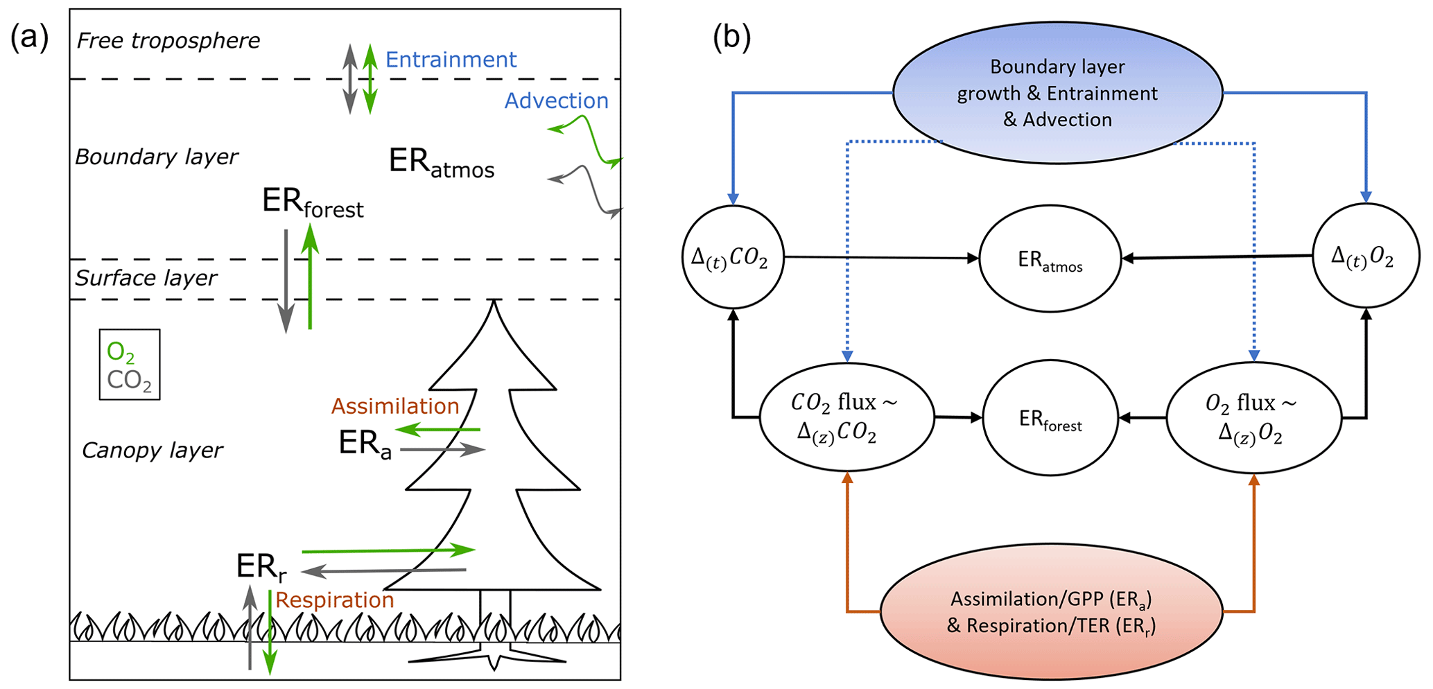
Figure 1Schematic overview of the different O2:CO2 exchange ratio (ER) signals, measured and analysed in and above a forest, influenced by the different O2 and CO2 fluxes and meteorological processes (a), together with a more detailed look on which processes influence the different ER signals (b). Panel (a) shows the direction of the surface fluxes during the day in the surface layer, which includes the roughness sublayer and the inertial sublayer. During the night the direction of the O2 and the CO2 surface fluxes are the other way around. The ER of the atmosphere (ERatmos) is determined from the change over time (Δ(t)) in the O2 and CO2 concentration measurements, and the ER of the forest (ERforest) is calculated from the surface fluxes of O2 and CO2, which are inferred from (∼) the vertical gradient (Δ(z)). ERa represents assimilation processes that influence the gross primary production (GPP) flux, and ERr represents respiration processes that influence the total ecosystem respiration (TER) flux. Panel (b) shows the connections between the processes, measurements, and the ERs. Dotted lines indicate smaller influences of the processes that are connected to it compared to solid lines.
On local/ecosystem scales, previous studies have shown that this terrestrial biosphere ER is not a constant value of 1.1 as used on the global scale and that it shows a certain degree of temporal and spatial variability. These studies either measured the oxidative ratios (ORs) from elemental composition analysis (Worrall et al., 2013; Randerson et al., 2006; Gallagher et al., 2017) or derived the ER from atmospheric concentration measurements (Battle et al., 2019; Seibt et al., 2004; van der Laan et al., 2014). Note that there is a distinction in the terminology between ER and OR. The OR indicates the stoichiometry of specific materials, whereas the ER indicates the exchange between the atmosphere and organisms or ecosystems. By using elemental composition analysis, the OR reflects the relationship between O2 and CO2 over a longer timescale of years or decades and only reflects the OR from the materials that are sampled. By using atmospheric concentration measurements for the ER, the ER reflects a shorter timescale compared to the OR of hourly to daily time periods, and it also reflects a different spatial scale, as the ER includes all processes that are originating from the footprint. The spatial scale that is covered by the ER signal depends on the type of measurements or modelling, i.e. leaf, canopy, or ecosystem. Both the OR- and ER-based studies showed that O2:CO2 molar ratio of the biosphere changes per ecosystem and over different time periods. The ER from the gas exchange experiments can furthermore be used for the separation of GPP and TER, using a specific ecosystem ER, which are determined with two alternative approaches (see Fig. 1) (Seibt et al., 2004; Stephens et al., 2007; Ishidoya et al., 2013, 2015; Battle et al., 2019). The first is the ER of the atmosphere (ERatmos), which is the ratio of the evolution of the atmospheric O2 and CO2 concentration measurements over time, and the second is the ER of the forest (ERforest), which is the ratio of the net surface fluxes of O2 and CO2 above the canopy, including all processes occurring below the canopy, including both vegetation and soil exchange. First attempts to estimate ERforest were made using one-box models (Seibt et al., 2004; Ishidoya et al., 2013). More accurate estimates of ERforest would be based on in situ measured O2 and CO2 surface fluxes; however, O2 currently cannot yet be measured accurately using EC techniques. Ishidoya et al. (2015) showed the first surface fluxes of O2 using vertical gradients of O2, an alternative technique to EC, and CO2 measurements at two heights above the canopy in the surface layer in a temperate forest in Japan. Their results showed that the ERforest signal could be used to separate the NEE signal into GPP and TER, consistent with the separation method for EC measurements using an empirical function of air temperature.
When using O2 to separately estimate GPP and TER fluxes, it is important to use the value for ER that represents ecosystem exchange. Seibt et al. (2004) showed that the signal of ERatmos cannot be directly linked to the exchange of carbon in the terrestrial biosphere, because in addition to the biosphere ERatmos is also affected by advection, boundary layer dynamics, and entrainment (Fig. 1). In contrast, Ishidoya et al. (2015) found similar values for ERatmos and ERforest. So far, there is no clear consensus on which signal should be used to indicate the ER of the ecosystem. Furthermore, since atmospheric O2 measurements are challenging to make, only a few studies exist that measured atmospheric O2 from flasks (Seibt et al., 2004) or continuously (Ishidoya et al., 2015; Stephens et al., 2007; Battle et al., 2019) above an ecosystem and derive ER signals. The uncertainty and spatial and temporal variability of O2:CO2 molar ratio of the biosphere are therefore not well known (Manning and Keeling, 2006; Keeling and Manning, 2014), and knowledge about the difference between ERforest and ERatmos, its variability across difference regions and ecosystems, and how ERforest can be used on both the local and global scale to advance our understanding of the carbon cycle is still limited. Therefore, more and longer in situ time series of atmospheric O2 measurements are needed, and further understanding of O2 and CO2 exchange above and below the canopy is crucial to continue the pioneering work by Seibt et al. (2004), Stephens et al. (2007), Ishidoya et al. (2015), and Battle et al. (2019) and to improve the application of the global biosphere ER, resulting in a better understanding of the carbon balance on local, regional, and global scales.
The aim of this study is to improve upon existing methods to calculate ERforest and get a better comparison of the ERatmos and ERforest signals. We carried out a measurement campaign in Hyytiälä, Finland, for two short periods in spring/summer 2018 and 2019 where both O2 and CO2 were measured at two heights with a setup including a differential fuel cell analyser for O2. We used our measurements to determine the diurnal behaviour of the relation between the concentrations and the fluxes of O2 and CO2, by using either one or both measurement heights on the tower. The objectives of this study are the following: (1) to extend the existing continuous O2 records, (2) to calculate the O2 surface fluxes in a boreal forest for the first time, (3) to combine the O2 and the CO2 fluxes (to calculate ERforest from these fluxes) and to compare the ERatmos and ERforest signals, and (4) to use ERforest to estimate GPP and TER fluxes.
In this paper, we first describe the measurement site, experimental setup, and methods used to derive O2 fluxes and the different ER signals (Sect. 2). We present the measurements for the whole campaign, and we select a representative day to determine the most suitable approach for deriving O2 fluxes and to determine ERforest (Sect. 3). A detailed evaluation and discussion of our ERatmos and ERforest signals is given in Sect. 4. We finalize with our conclusion about the diurnal variability of the ER signals for a representative day of a boreal forest (Sect. 5).
To determine ERatmos and ERforest (and its diurnal variability), we measured O2 and CO2 continuously at two heights above a boreal forest during two short campaigns at Hyytiälä. These OXHYYGEN (oxygen at Hyytiälä) campaigns took place in the spring/summer of 2018 (3 June through 2 August) and 2019 (10 June through 17 July). In this section, we describe the measurement site and instrumental setup, as well as the methods used to determine the O2 and CO2 fluxes from the measured vertical gradient and the ER signals.
2.1 Measurement site
The measurements were made at Hyytiälä SMEAR II forestry station of the University of Helsinki in Finland (61∘51′ N, 24∘17′ E; +181 ; time zone: UTC+2); this site is described in more detail in, for example, Hari et al. (2013). The SMEAR II station is a boreal site within the European Integrated Carbon Observation System (ICOS) network with atmospheric and ecosystem measurements. The SMEAR II station is located inside a homogeneous forest of Scots pine trees (Pinus Sylvestris) with a dominant canopy height of 18 m and some silver birch and aspen trees. The forest floor is covered with mosses and herbs. The soils are podzols on top of glacial till. A large lake is located close (around 550 m) to the measurement site and has a fetch of 250 m over the dominant wind direction of 230∘. The footprint of the site is mostly influenced by natural sources, with the atmospheric signal dominated by forest exchange (Carbon Portal ICOS RI, 2022). The measurement site includes several towers, including a 128 m tall tower and a 23 m high walk-up tower, where atmospheric variables and gas concentrations are continuously measured. The operational data from this tower are publicly available online at http://avaa.tdata.fi/web/smart/smear/ (last access: 5 January 2022). Our O2 and CO2 measurement setup was installed in a cabin at the bottom of the 23 m high tower, and air was sampled from aspirated inlets (Blaine et al., 2006), installed at 23 m in the smaller tower and at 125 m in the tall tower, which are 5 and 107 m above the canopy height, respectively. We used both levels to calculate the vertical gradient for the flux calculations (Sect. 2.3).
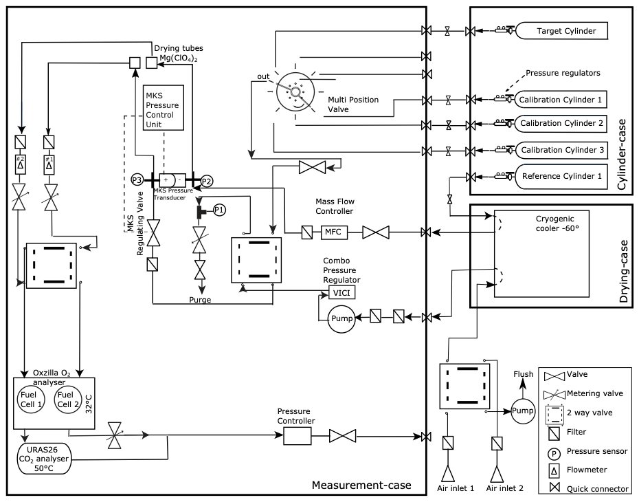
Figure 2Schematic overview of the measurement setup used at Hyytiälä. The setup includes an Oxzilla O2 fuel cell analyser and a URAS26 NDIR CO2 analyser. The system measured air sampled from two heights of either 23 or 125 m.
2.2 Experimental setup
The measurement setup is based on the instrument used in van Leeuwen and Meijer (2015), following the methods in van der Laan-Luijkx et al. (2010) and Stephens et al. (2007). O2 is measured with a Sable Systems Oxzilla II fuel-cell-based instrument, and CO2 is measured with an ABB continuous gas analyser URAS26, which is a non-dispersive infrared (NDIR) photometer. The gas-handling schematic is shown in Fig. 2.
Air was pumped from either 23 or 125 m height to the measurement system at the base of the tower. Both inlet lines were continuously flushed, where either one of the heights is measured by the system with a sample flow of around 120 mL min−1 and the other flushed to the room with a higher flow rate of around 2 L min−1, which allows for fast switching between the two heights. We switched between the inlets every half hour to match the EC measurements of ICOS that were already present in the tower and to get a more stable signal of O2. The air of the selected inlet was first cooled to −60 ∘C with a cryogenic cooler to remove water vapour from the air, before entering the system. Second-stage drying of the air streams was done with magnesium perchlorate (Mg(ClO4)2) traps. The sample air was continuously measured against a reference gas (differentially for O2 and alternatively for CO2), and the pressure in both sample and reference lines was matched to be the same using a pressure control system (MKS Instruments, types 223B, 248A, and 250E for the pressure transducers, regulating valve, and control system, respectively). The reference and sample lines were switched every 2 min between the two fuel cells in the Oxzilla analyser. We measured a set of three calibration cylinders and one target cylinder every 23 h for half an hour per cylinder.
The measurements of these calibration gases allowed for calibration of our measurements against the international Scripps Institution of Oceanography (SIO) scale for . We did that by using cylinders that are filled in the laboratory at the University of Groningen, where they were calibrated with the primary Scripps cylinders (Nguyen et al., 2022). The O2 measurements are normally expressed as ratios in “per meg” instead of mole fraction (ppm), since O2 is not a trace gas because of its high abundance of 20.95 %; therefore, the mole fraction varies due to changes in other gases, such as CO2 (Keeling et al., 1998). So is defined as
For simplicity, in this paper we use the term O2 instead of , and we use the term “concentration” rather than “mole fraction” when discussing both CO2 and O2. Equation (3) indicates a change compared to a reference level. Negative values therefore indicate concentrations of O2 lower than the reference value. To allow for comparison of changes in CO2 and O2 directly, we converted the units of O2 from per meg to ppm equivalents (ppmEq), where a change of 1 ppm CO2 corresponds to a 4.77 per meg change in O2 (Tohjima et al., 2005; Kozlova and Manning, 2009).
We modified the method described in van der Laan-Luijkx et al. (2010) to calibrate the measurements. The raw CO2 measurements have a frequency of one measurement per 6 s, the raw O2 measurements have a frequency of one measurement per second, and both give one value every 4 min in the form of ΔCO2 and Δ(Δ)O2, respectively. CO2 is measured on a single cell instrument; therefore, ΔCO2 is the difference between the 2 min averages of the sample air (S) and the reference cylinder (R), giving (S−R). For the 2 min averaged CO2 measurements, the last 78 s of each 2 min period were used. Note that for CO2, the NDIR system is different compared to other systems used and therefore does not need a zero gas (Pickers et al., 2017). O2 is measured on a double-cell instrument and therefore gives a double differential signal. The Δ(Δ)O2 value is the difference between the 2 min averaged difference between S and R and the 2 min averaged difference between R and S (). For the 2 min averaged O2 values, the last 100 s of each 2 min period are used. In 2019, the MKS pressure control valve was not functioning optimally, which led to a small instability in the differential pressure between the sample and reference lines. We therefore corrected the 4 min values of Δ(Δ)O2 for this deviation measured by the MKS differential pressure sensor (PMKS) by multiplying Δ(Δ)O2 with (0.095 × PMKS), which we derived based on the measurements of the calibration cylinders. In 2018, there was no instability in the pressure control valve; therefore, no correction was applied in that year. The PMKS deviations correlated with temperature and increased towards the end of the 2019 campaign. Figure B1 in Appendix B shows that the highest corrections were made during midday at the end of the campaign. The O2 vertical gradient is hardly affected by the correction as it is the difference between measurements at two heights that are both undergoing the same deviation.
For both CO2 and O2, the 4 min values were subsequently used to calculate half-hourly means, where we excluded the first 4 min value after the heights are switched, together with the measurements that did not fall inside the boundary based on the median absolute deviation (MAD) (Rousseeuw and Verboven, 2002). For every half-hourly mean, a standard error is calculated (see Eq. 4), which is used in further analysis to determine the uncertainty of our measurements.
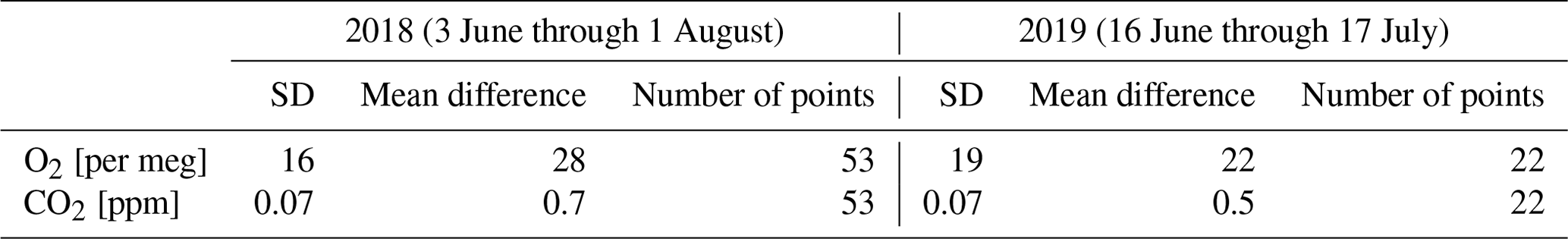
The linear calibration response functions for both O2 and CO2 were calculated for every measurement period of the calibration cylinders, which was about every 23 h. For the response functions, we used a constant slope based on the mean of all the calibration slopes measured in the specific year. The y intercept values of the response functions were interpolated to the time of the measurement, based on the two calibrations bracketing the measurement time. To facilitate the comparison of the O2 and CO2 measurements of the two heights and allow for flux calculations based on the vertical gradient, we interpolated the data to one measurement for every 30 min for each height. Based on the target cylinders, measured during the calibration period, the stability of the long-term measurements was determined (Table 1). A different target cylinder, with different composition of air for 2019 compared to 2018, was used, which resulted in different outcomes for the standard deviation (SD) and the mean difference for these periods. The mean difference is calculated from the target measurements at Hyytiälä compared to the calibrated values using the SIO cylinders in Groningen. The measurement period of 2018 was also longer and so more points were included for the SD and mean difference calculations. The long-term measurement precision of this device throughout the duration of the two measurement campaigns compared to the recommendations of the World Meteorological Organization (WMO) will be further discussed in Sect. 4.1.
Table 1The mean difference and the standard deviation (SD) of the target cylinder measurements of O2 and CO2 for the 2018 and 2019 periods separately, together with the number of data points used to calculate these specific values.
2.3 Data analysis
For the analyses presented in this paper, we needed representative diurnal cycles of O2 and CO2. We looked for a representative day in 2019 when little to no clouds were present; no unexpected behaviour in the diurnal cycles for potential temperature, specific humidity, or CO2 occurred (e.g. caused by advection); and when the O2 data showed a clear difference between the two measurement heights. We used data from 2019 instead of 2018 as 2018 saw a large-scale drought in Europe, and 2019 was less extreme and closer to a typical boreal summer (Peters et al., 2020). However, no single representative day could be found in our 2019 record, when the O2 data showed a clear negative vertical gradient during the day and positive during the night, in combination with the above-mentioned meteorological criteria. We therefore choose a sequence of days to create an aggregate day based on the average of several days, which is representative for this time of the year in Hyytiälä, following the same method used by Ishidoya et al. (2015). The main criterion was that the vertical O2 gradient had to be negative during the day, and the negative relationship between the change of O2 and CO2 concentrations over time at 23 m was present during the entire day. This resulted in selecting the period of 7 through 12 July 2019 to create the representative day, which we used in all subsequent analyses. The half-hourly values for the representative day are the averages of the data points of the individual half-hourly values for each day in the selected period. Each time step has an uncertainty that is based on the error propagation of the standard error (SE) of the 30 min averages for each day in the aggregate and is calculated for each time step with
where n is the number of days included in the aggregate, SEday is the standard error of the 30 min average of each individual day, and the SEaggr is the resulting standard error of a 30 min value for the representative aggregate day.
For the representative day, the two O2:CO2 exchange ratio (ER) signals, ERatmos and ERforest, were determined. ERatmos is based on O2 and CO2 concentrations and is expressed as
where both Δ(t)O2 and Δ(t)CO2 are the change in concentration over a selected time period (t). This is a unitless quantity as it represents mol O2 per mol CO2. ERatmos was determined by the slope of a linear regression between the concentration of O2 and CO2 at the same height over a specific time period (Seibt et al., 2004; Stephens et al., 2007; Ishidoya et al., 2013; Battle et al., 2019). The selected time periods were based on the period when O2 and CO2 had the highest negative correlation. Throughout the day, this could be divided into three periods when different processes dominate (Fig. 1). It starts with the period during the night when the atmosphere is stable and when respiration becomes the dominant surface flux (P1); therefore, the CO2 concentration increases and the O2 concentration decreases. Subsequently, when the sun starts to rise, the boundary layer height starts to grow, and entrainment of air from the free troposphere influences the surface measurements (P2) (Vilà-Guerau de Arellano et al., 2004). Here the CO2 concentration decreases rapidly and the O2 concentration increases rapidly. Finally, the period starts when the effect of boundary layer dynamics and entrainment decreases, and the assimilation flux dominates (P3); here, the CO2 concentration decreases less rapidly and the O2 concentration increases less rapidly. We calculated an ERatmos signal with Eq. (5) for the nighttime (P1), the daytime (by either focusing on only P3 or both P2 and P3), and the complete day (P1 + P2 + P3). The exact boundaries of these periods have to be estimated. To be certain about the exact times that should be taken as the boundaries for each period, an atmospheric model is needed.
ERforest is based on O2 and CO2 fluxes and is expressed as
where and are the net mean turbulent surface fluxes above the canopy of O2 and CO2 over a selected time period (Seibt et al., 2004; Ishidoya et al., 2015). We derive the fluxes of O2 and CO2 using the vertical gradient (see next paragraph and Eq. 7). The selected time periods for ERforest were chosen such that the transition periods between the nighttime with a stable atmosphere (when the respiration flux dominates) and the daytime with a well-mixed atmosphere (when assimilation dominates) were excluded. By excluding the transition periods, we removed the periods when the gradients of both CO2 and O2 were close to zero. This was done because a very small gradient makes it difficult to calculate a flux and therefore the ERforest and also because during this period entrainment is the most dominant process. The exact duration of the transition periods was based on the maximum and minimum of both the friction velocity and the height of 27 m (z) divided by the Monin–Obukov length (L). The friction velocity and () indicate the measure of turbulence of the atmosphere (Stull, 1988). The mean of the remaining data points of the CO2 and O2 flux during the stable atmosphere period was used to calculate the ERforest signal of the night, and the mean of the remaining data points of the CO2 and O2 flux during the mixed atmosphere period was used to calculate the ERforest signal of the day. The ERforest for the entire day is taken as the average CO2 and O2 flux over the entire day. For this average, no periods are excluded, and all the data points over the 24 h are taken into account. Taking the average daily fluxes to derive ERforest is a slightly different approach compared to the study by Ishidoya et al. (2015), who use the regression line between Δ(z)O2 and Δ(z)CO2 to determine ERforest.
Currently, unlike for CO2, the O2 flux cannot be measured directly with an EC system. Instead, the flux can be inferred from the flux-gradient method. To calculate the flux of a certain scalar (ϕ) with the flux-gradient method, the following equation was used (Stull, 1988):
where Fϕ is the surface flux of ϕ, K is the exchange coefficient, and is the vertical gradient of . To determine the O2 flux with Eq. (7) (where ), the exchange coefficient of O2 () needs to be determined. Ishidoya et al. (2015) assumed that and determined by dividing the CO2 flux, measured with EC, by the CO2 vertical gradient between two measurement levels. However, the exchange coefficient can also be determined with other methods that, for example, only need two measurement heights for the vertical gradient. In this study, we explore these different options for calculating . The EC measurements of the CO2 flux were used as a reference to determine the most suitable approach. The most suitable approach to infer the O2 flux is then used for both and . During this study, we derive the surface flux in the surface layer (Fig. 1), and we assume that the surface flux stays constant in this surface layer, which consists of the roughness sublayer and the inertial sublayer.
We categorized the methods to determine the most suitable K into two groups: the observation-based approach (also called the K-theory (Stull, 1988) or the modified Bowen ratio method (Meyers et al., 1996)) and the theoretical approach (following the similarity theory (Dyer, 1974)). For the observation-based methods, we determined the exchange coefficient (K) in Eq. (7) by dividing a flux measured at 27 m, using an EC system, by a three-height (16, 67, and 125 m) vertical gradient of a specific scalar. Ishidoya et al. (2015) used this approach to calculate their O2 flux, using the CO2 flux and vertical gradient of two levels. Next to CO2, we also calculated K using potential temperature (θ) for the observation-based approach.
For the theoretical approach, the K in Eq. (7) is determined with the Monin–Obukov similarity theory (MOST) (Dyer, 1974), where logarithmic surface layer scaling applies for K, and empirical similarity functions are used to describe the effect of atmospheric stability. In addition, we used a correction which takes into account the effect of the roughness sublayer (see Appendix A for details). The SMEAR II data at 27 m were used for the calculations with MOST. When only two heights for the gradient calculations are available, there is an option to integrate Eq. (7) (de Ridder, 2010). We tested both the application with and without integration in this study. We used the ICOS data, available at the SMEAR II station, for the K calculations. For the CO2 EC measurements, we used the gap-filled data to correct for the storage below the measurement height of the EC. Gap filling was applied when the friction velocity (u*) was below 0.4 m s−1 (Kulmala et al., 2019). Appendix A gives a more elaborate explanation and provides equations of the different methods used to determine the exchange coefficients used in this study.
Finally, we select the Kϕ from either the observation-based or the theoretical approach that produced CO2 flux results from our CO2 vertical gradient measurements that showed the best comparison to the EC CO2 flux measurements. This K was used to calculate the O2 and CO2 fluxes, together with the vertical gradient from measurements collected during our campaigns. For our campaigns, we only have O2 and CO2 measurements at two heights (23 m and 125 m), which means that changes into , and the gradient was calculated with finite differences.
After both the CO2 and O2 fluxes were determined, resulting in ERforest, we subsequently calculated the O2 : CO2 exchange ratio signals for the assimilation processes (ERa) and the respiration of the ecosystem (ERr) with the following equations (Seibt et al., 2004; Ishidoya et al., 2015):
where NEE is the net ecosystem exchange, GPP is the gross primary production, and TER is the total ecosystem respiration. GPP and TER are always positive by definition, representing uptake and release by the ecosystem, respectively. Therefore, when GPP is larger than TER the resulting negative NEE values represent carbon uptake by the ecosystem. First, we assumed that nighttime NEE is equal to TER, which meant that the nighttime ERforest signal is equal to ERr. We assumed that the processes that contributed to the ERr keep the same ratio between O2 and CO2 during the entire day and therefore we used a constant ERr for the entire day. We base this assumption on studies that showed that the variability of ERr highly depends on the bulk soil respiration (Hilman et al., 2022; Angert et al., 2015). No large changes occur in the soil temperature or the soil moisture during our (representative) diurnal cycle; therefore, we assume that the ERr of the bulk soil respiration stays relatively constant, and with that the ERr of the ecosystem also stays constant over the entire day. Subsequently, we calculated ERa for both the entire diurnal cycle and the daytime using Eq. (9) with the corresponding ERforest and the constant ERr. We used ICOS NEE EC measurements from the SMEAR II station at a level of 27 m in the 128 m high tower. The GPP fluxes at Hyytiälä are calculated with either of the following two approaches: (1) when NEE EC measurements are available, GPP is calculated as the difference between the NEE EC measurements and the respiration flux, which is calculated using a temperature function; or (2) when NEE EC measurements are not available, GPP is calculated using an equation that is based on the air temperature and light (photosynthetically active radiation, PAR). A more detailed description of these calculations is given by Kulmala et al. (2019) and Kohonen et al. (2022).
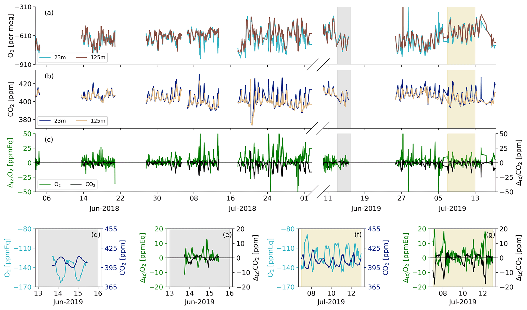
Figure 3The half-hourly average O2 (a) and CO2 (b) concentrations at Hyytiälä for spring/summer of 2018 and 2019 for the 125 and 23 m height levels, together with the vertical gradient (Δ(z)) between these two heights (c) for both O2 and CO2. The shaded areas indicate the dates that were selected for the aggregate representative day (7 through 12 July 2019: yellow) and the second representative day to test the O2 method (13 through 15 June 2019: grey). The selected days for the aggregate representative days are shown in more detail for the 23 m measurements for the gradients during 13 through 15 June (d) and (e) and during 7 through 12 July (f) and (g) for both O2 and CO2.
By estimating ERr and ERa of this boreal forest, we created the opportunity to apply atmospheric O2 measurements to separate NEE into GPP and TER (the O2 method). We calculated ERr and ERa for the representative day using Eqs. (8) and (9), and we use these to calculate GPP and TER for another representative day. We selected 13 through 15 June to create a new second aggregate day and to calculate a new ERforest signal for the entire day (see Fig. 3d and e for a detailed view on the measurements of those days). These three days were chosen because in 2019 they showed the clearest diurnal cycle of O2 and a negative O2 gradient, aside from 7 through 12 July, used above. We assume here that the ERr and ERa calculated for the period from 7 through 12 July are representative for the period from 13 through 15 June. Studies show that the ERr (Hilman et al., 2022) and ERa (Bloom, 2015; Fischer et al., 2015) values vary with changing soil and atmospheric conditions. The periods for both representative days are relatively close in time and therefore have similar conditions in the soil and the atmosphere, and we can therefore assume that the ERr and ERa values based on the 7 through 12 July data can also be applied to the 13 through 15 June period. By using the ERr and ERa values determined for the first representative day (7–12 July) and ERforest and NEE for the second representative day (13–15 June), we calculated GPP and TER from NEE for this second representative day. By comparing the GPP and TER fluxes of the O2 method to the GPP and TER fluxes of the temperature-based function of ICOS (EC method), we could demonstrate how accurate the O2 method is (Sect. 3.4). Both Seibt et al. (2004) and Ishidoya et al. (2015) also applied the O2 method; however, both of these studies used chamber measurements to first determine ERa and ERr and then used Eqs. (8) and (9) to infer GPP and TER. Unfortunately, we did not have chamber measurements of both O2 and CO2 available and therefore we used Eqs. (8) and (9) to calculate ERa and ERr. This means that these two equations can be used in two ways: to determine the ERa and ERr signal or to separate NEE into GPP and TER.
The footprint of the calculated O2 and CO2 surface fluxes that also represents the footprint of the ERforest, ERr, and ERa signals for the representative aggregate day is shown in Fig. B2 in Appendix B. The footprint is based on the method by Kljun et al. (2015), where for the height the geometric mean between 125 and 23 m is used. The footprint analysis shows that the surface fluxes are mainly influenced by the forest surrounding the tower and that the lake located close to the tower is not influencing the signal. The footprint of the O2 and CO2 concentrations and therefore the footprint of the ERatmos signal can be found in the document by Carbon Portal ICOS RI (2022). This concentration footprint analysis shows that with an average wind direction of north to northeast during 7 through 12 July 2019, the concentrations measured are mainly originated from forest exchange, with hardly any influence of urban sources.
Table B1 in Appendix B gives a complete overview of which data are used for each part of this research for the two different aggregate days.
3.1 O2 and CO2 time series
The calibrated half-hourly measurements of O2 and CO2 for 2018 and 2019 are shown in Fig. 3, together with the vertical gradients between the two measurement heights. The O2 measurements are shown here converted from per meg to ppmEq, which is to allow for comparison of the diurnal variability for CO2 and to calculate the ER signals. The differences between the 23 and 125 m measurements are observable for both CO2 and O2. During both campaigns in 2018 and 2019, the diurnal behaviour of the O2 concentrations are anticorrelated with the CO2 concentrations. This anticorrelation between O2 and CO2 is also visible from the gradient measurements, despite the relatively high uncertainty of the O2 measurements as described in Sect. 2.2 and further elaborated on in Sect. 4.1. The period 7 through 12 July 2019 shows the most clear negative relationship between the O2 gradient and the CO2 gradient, and it also had the most suitable meteorological conditions and was therefore selected for the aggregate representative day (Sect. 2.3). The period 13 through 15 June shows a less clear anticorrelation between the vertical gradients of O2 and CO2 (Fig. 3d and e) but with clear diurnal cycles of O2 and CO2 suitable for the purpose of our second aggregate day (see Sect. 3.4).
3.2 Diurnal cycles
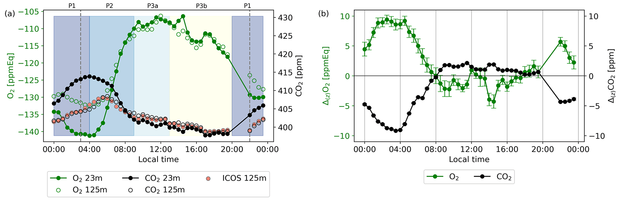
Figure 4Diurnal cycles in local wintertime (LT; time zone UTC+2) (all times in this paper are given in local time unless stated otherwise) of the O2 and CO2 concentrations for the 23 and 125 m height levels (a) and the vertical gradient between both levels with the uncertainty of both O2 and CO2 of the representative day, taken as the average values of 7 through 12 July 2019 (b). The CO2 measurements of the ICOS setup are shown in (a) for comparison with the CO2 setup measured during our campaigns. The shaded colours indicate the selected different periods when the most dominant processes are the following: stable atmosphere and respiration (00:00–04:00, P1); entrainment, boundary layer growth, and assimilation (04:00–09:00, P2); convective conditions and assimilation (09:00–13:00, P3a); and the same as P3a plus a remaining artefact for the O2 measurements after the pressure correction as explained in the text (13:00–20:00, P3b). The vertical dotted lines indicate the sunrise (03:00) and sunset (22:00). The error bars in panel (b) are half-hourly standard errors based on the error propagation of the standard errors of the data points in (a) (not shown), which were based on Eq. (4).
The measurements of O2 and CO2 and their vertical gradient for the representative day, are shown in Fig. 4. There are no measurements between 20:00 and 22:00, because the calibration cylinders were measured during this period. For 7 through 12 July, we used a fixed calibration time, as radiosondes were launched (not shown) during this period, and we wanted to make sure we captured the morning transition to compare with these radiosondes. Note that the daylight length at Hyytiälä is long at this time of the year, with sunrise at 03:00 and sunset at 22:00. We compared our CO2 observations with ICOS CO2 measurements at the same height, which shows that both instruments compare well overall, with a mean difference of 0.70 ± 0.65 ppm during the period 7 through 12 July. The comparison between the two devices was a bit difficult because of the different timing of the measurements. The diurnal cycles of O2 and CO2 (Fig. 4a) clearly show anticorrelated behaviour between CO2 and O2, which is especially visible during nighttime (23:00–04:00) and the morning transition (05:00–13:00).
Figure 4 shows four different periods that can be linked to the periods to calculate ERatmos, described in Sect. 2.3. P1 is visible between 23:00–04:00, where respiration starts to dominate the signal and therefore the O2 concentration decreases and the CO2 concentration increases, in a decreasing boundary layer height dominated by thermal stratification. P2 becomes visible around 04:00 and stops around 09:00, where entrainment, the growing boundary layer, and the onset of photosynthesis causes a steep increase in the O2 concentration and a steep decrease in the CO2 concentration. P3 can be divided into P3a and P3b and is visible between 09:00–20:00. Between 09:00–13:00 (P3a), the photosynthesis flux starts to dominate, and both the O2 and CO2 concentration increase and decrease less rapidly. Between 13:00–20:00 (P3b), the O2 concentration starts to decrease while the assimilation flux still dominates, which is a remaining artefact from the pressure correction that we applied due to the instability of the MKS pressure transducer (see Sect. 2.2). As shown in Fig. B1 in Appendix B, higher daytime temperatures cause larger PMKS deviation and therefore the effect of the pressure correction is largest during midday, leading to a larger uncertainty in the observations in that time period. The boundary of 20:00 between P3b and P1 was difficult to determine as we missed some measurements due to the calibration period, and the remaining measurements around this time have a deviation caused by the pressure transducer. Measurements at both levels show this same diurnal behaviour; however, it is more pronounced closer to the vegetation (the 23 m level).
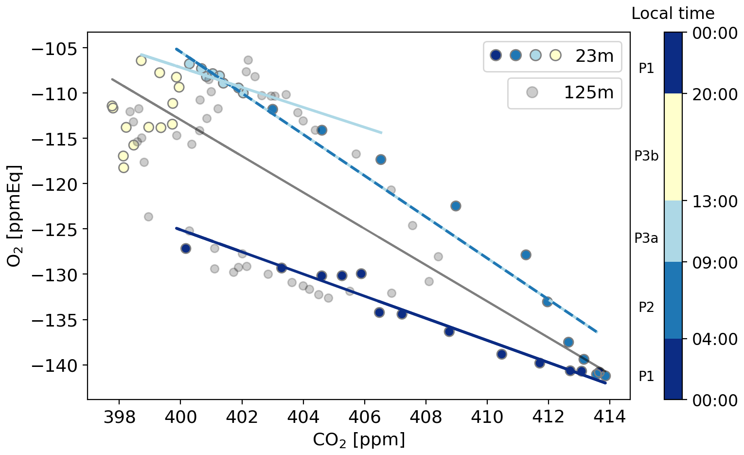
Figure 5The O2 concentration plotted against the CO2 concentration for the representative day in local wintertime (LT; time zone UTC+2), with the 23 m level in coloured points per period representing different dominant process and with the 125 m level in grey points. The dominant processes are the following: respiration (00:00–04:00), entrainment (04:00–09:00), assimilation (09:00–13:00), and a remaining artefact after the pressure correction due to the instability of the MKS pressure transducer becomes visible (13:00–20:00). The linear regression lines indicate the exchange ratio of the atmosphere (ERatmos) during the time with a specific dominant process.
The difference between the two heights results in a vertical gradient (Fig. 4b). Similar to the diurnal cycle of the concentrations, the diurnal cycles of the gradients of O2 and CO2 also show anticorrelated behaviour. At 08:00, the CO2 gradient changes from negative to positive, and the O2 gradient changes from positive to mostly negative, reflecting CO2 being transported downwards and O2 upwards, respectively. The magnitude of the gradient depends on the degree of vertical mixing. The sign of the gradients changes during the day, because the lowest level (23 m) is more directly influenced by forest carbon exchange compared to the highest level (125 m). Around the time of sunset, the CO2 gradient changes from positive to negative, and the O2 gradient changes from negative to positive, because the lowest measurement level (23 m) is now influenced more by respiration processes of the forest and soils compared to the highest measurement level (125 m). The error bars are based on the error propagation of the standard errors of each half-hourly data point that were calculated with Eq. (4). The gradient of O2 is hardly affected by the PMKS correction (see Fig. B1), as measurements at both heights are affected similarly.
By using Eq. (5), we calculated four distinct ERatmos signals for different periods throughout the day at 23 m, as well as to a smaller degree at 125 m (Fig. 5 and Table 3). The same periods as shown in Fig. 4 are visible in Fig. 5. This results in an ERatmos during the night (P1) of 1.22 ± 0.02 and two different possibilities for the ERatmos signal during daytime. By combining both P2 and P3a, we get a signal of 2.28 ± 0.01, and by focusing only on P3a, which excludes the entrainment and the boundary layer dynamics, we get a signal of 1.10 ± 0.12. Last, by combining all the periods (P1, P2, P3), we get a signal for the complete day of 2.05 ± 0.03. The uncertainties given here only represent the uncertainty of the slopes from the regression lines in Fig. 5. The high values for the ERatmos signal of the entire day and the daytime signal that includes entrainment and the boundary layer dynamics are not very realistic to represent an ER for the forest, and this shows that we should be careful when using ERatmos. This will be elaborated on in Sect. 4.2.
3.3 Flux calculations for CO2 and O2
We explored four alternative methods to derive the O2 flux from the vertical gradient of the two measurement levels, as described in Sect. 2.3. Figure 6 shows both the theoretical and the observation-based approaches that were used to calculate the CO2 flux, in comparison to the ICOS EC CO2 flux measurements at 27 m on the tower. By comparing these approaches to the EC measurements, we determined which method is most suitable to calculate the O2 flux. The CO2 flux measured by the EC system stays positive until around 05:00, when the respiration fluxes are the most dominant and the nocturnal boundary layer is shallower. After 05:00, the CO2 flux of the EC system becomes negative, and the forest begins to take up CO2 instead of emitting it. The assimilation fluxes increase and exceed the respiration fluxes, the boundary layer starts to grow, and air with lower CO2 concentrations is entrained from the free troposphere. After 20:00, the CO2 flux of the EC system becomes positive again as the assimilation fluxes decrease, and the respiration signal begins to dominate again while the boundary layer height decreases. We expect to find this diurnal pattern and the sign change in our calculations of the CO2 flux from the vertical gradient method as well.
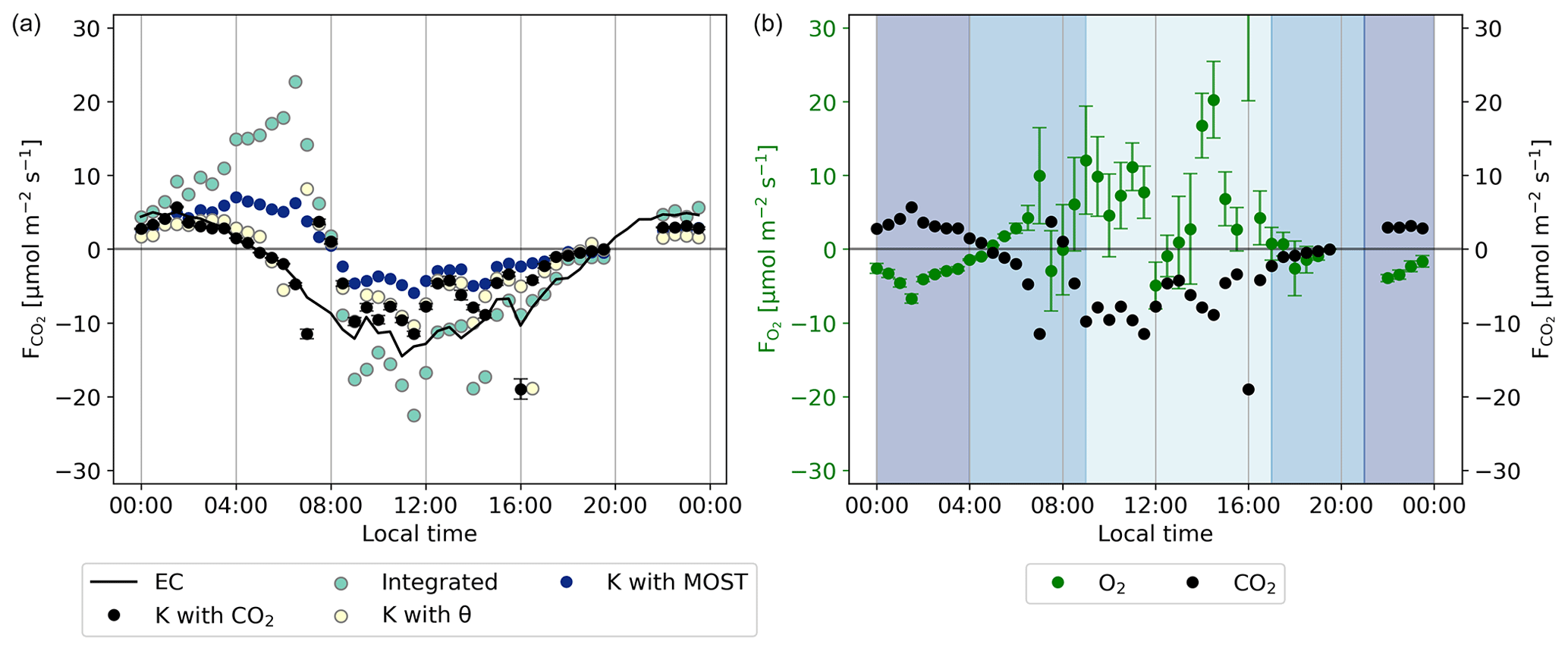
Figure 6The CO2 flux (a) calculated with different methods for the representative day, as described in Sect. 2.3, compared to the CO2 flux of the ICOS EC measurements. (b) The comparison between the O2 and CO2 flux calculated using the method that gave the best results for the CO2 flux calculations (using the exchange coefficient K with CO2) for the representative day. The shaded colours indicate the regions that were selected for the following: the night signal (21:00–04:00), the day signal (09:00–17:00), and the remaining regions (04:00–09:00 and 17:00–21:00), with the time in local wintertime (LT; time zone UTC+2). The error bars of (b) are based on the error propagation of the standard error of the 30 min values for the representative day, which are based on Eq. (4).
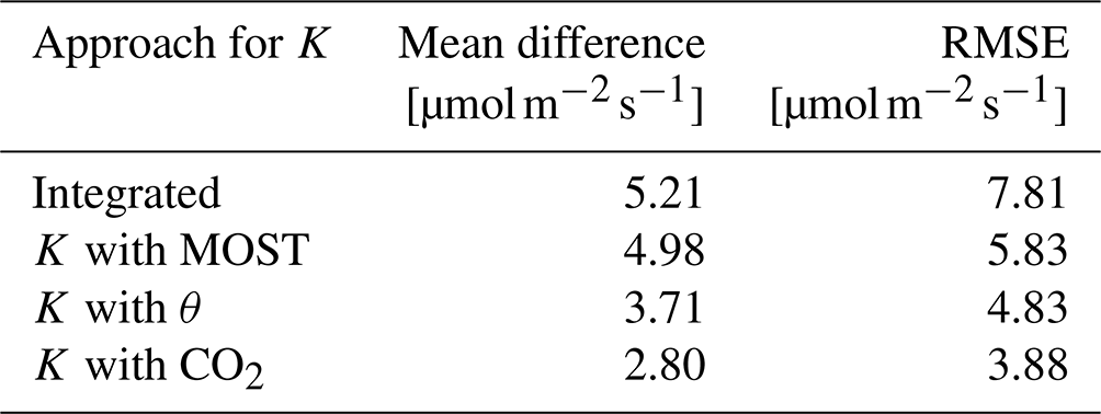
First, we discuss the theoretical methods that are indicated in Fig. 6 with “K with MOST” and “Integrated” approaches (see Sect. 2.3). The MOST and the integrated methods both overestimate the CO2 flux during the night, between 0:00 and 05:00. In addition the resulting CO2 flux decreases and becomes negative too late in the day compared to the EC measurements. The CO2 fluxes of the MOST and integrated methods evolve from a positive flux to a negative flux around 8:00. This is 3 h later than the CO2 flux from the EC measurements. During the day, between 08:00 and 15:00, the MOST method underestimates the CO2 uptake and the integrated method overestimates it. Table 2 shows that both MOST and the integrated methods have the highest mean difference and root mean square error (RMSE) compared to the observation-based approaches. We discuss this further in Sect. 4.3. As a result of this analysis, we decided to not use the theoretical approach to calculate the O2 flux.
Table 2The mean difference and the root mean square error (RMSE) of the comparison between the EC CO2 flux measurements at 27 m in the tower and the CO2 flux calculated with different methods for the exchange coefficient K, based on the ICOS data, each using the vertical gradient of CO2 at 23 m and 125 m of our campaign data.
Secondly, we analyse the observation-based approaches that are indicated in Fig. 6 with “K with θ” (where K is established using ICOS vertical gradients of potential temperature and the sensible heat flux) and “K with CO2” (where K is established using ICOS CO2 vertical gradients and CO2 EC data). The observation-based approaches showed a better comparison with the EC observations in determining the CO2 flux compared the to theoretical approach. Both the θ and the CO2 methods represent satisfactorily the nocturnal CO2 flux between 00:00 and 05:00. After 05:00, the fluxes calculated by both methods start to decrease and change sign around the correct time (05:00) from a positive to a negative flux. During the day between 08:00 and 15:00, both the θ and the CO2 methods underestimate the CO2 flux but not as much as the theoretical methods. Table 2 also shows that both the θ and the CO2 methods have the lowest mean difference and RMSE. Based on the smaller mean difference and RMSE, as well as the direct link of CO2 with O2, we decided to proceed with the method where K is calculated with the ICOS data of CO2 instead of the ICOS θ data. This K was then multiplied with our measured O2 vertical gradient between 23 and 125 m to calculate the O2 flux. Section 4.3 presents a more complete discussion on the different methods to determine the most suitable K.
The resulting O2 flux calculated with the exchange coefficient K based on the ICOS CO2 data is shown in Fig. 6b. The uncertainties are based on the error propagation of the standard errors of the O2 and CO2 data per time step as calculated with Eq. (4), in Eq. (7). We do not calculate an uncertainty for K, as this is not the dominating term contributing to the total uncertainty. The daytime flux values have a high variability, but the inferred fluxes appear physically realistic and promising for one of the first attempts to calculate O2 fluxes. During the night, between 0:00 and 5:00, the O2 flux signal has a relatively stable negative value, because the forest consumes O2 for the respiration processes. Similarly, CO2 is released during the night, leading to a positive CO2 flux. After 5:00, the O2 flux becomes positive and shows a higher variability. Overall, the O2 flux is positive during the day, which indicates that the forest produces O2 as the assimilation rate is higher than the respiration rate. The high variability of the O2 flux compared to the CO2 flux is caused by the less precise measurements of the O2 vertical gradient compared to the CO2 gradient (Fig. 4). The measurement precision needed to measure the difference between the two levels is very high and therefore impacts the measurement of the gradient of O2. The nighttime values of the O2 flux are therefore more reliable than the daytime values, since the difference between the two heights is larger and due to the more stable atmospheric conditions at night.
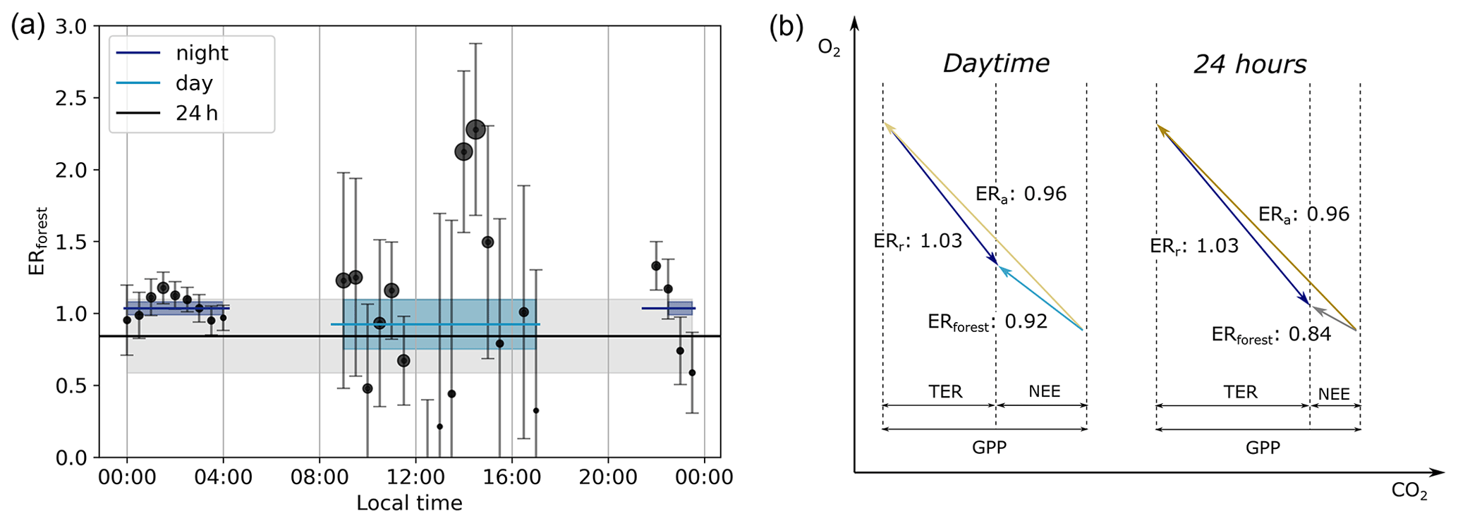
Figure 7The half-hourly exchange ratio of the forest (ERforest) and the resulting averaged ERforest for the entire day (black line), the night between 21:00–04:00 (dark blue line), and the day between 09:00–17:00 (light blue line) of the representative day (a) with the time in local wintertime (LT; time zone UTC+2). The size of the dots indicates the size of the absolute O2 flux, and the shaded bands indicate the uncertainties of the different ERforest signals. Note that the ERforest lines do not match with the average of the dots in the specific time period, because the lines are based on the averaged fluxes. These different ER signals are presented in a vector diagram format with the carbon fluxes, gross primary production (GPP), total ecosystem respiration (TER), net ecosystem exchange (NEE), the ER of the assimilation processes (ERa), and the ER of the respiration processes (ERr) (b).
By using Eq. (6), we find three different ERforest signals throughout the day (Fig. 7 and Table 3). The selected time periods based on the criteria described in Sect. 2.3 are between 09:00–17:00 for the daytime and between 21:00–04:00 for the nighttime (Fig. 6). This results in a nighttime ERforest signal of 1.04 ± 0.04, a daytime ERforest signal of 0.92 ± 0.17, and an ERforest signal for the entire 24 h of 0.83 ± 0.24. Note that this 24 h value is not the average of the day and night ERforest signals or from all the 30 min ERforest signals, because we used the averaged fluxes. This means that the ERforest signals based on high flux values, indicated in Fig. 7 with larger symbols, contribute more to the averaged ERforest signals compared to the lower flux values. Figure 7b illustrates that when combining surface fluxes with different sign, we cannot just average the corresponding ER signals (see Sect. 4.4). The individual ERforest values of every 30 min show a clear difference between the daytime and nighttime. The ERforest values during the nighttime are relatively stable. The ERforest values during the daytime show more variability, caused by the high variability of the O2 flux during daytime (Fig. 6). The uncertainty of the ERforest signals is determined by the propagation of the standard error of the aggregate 30 min data (based on Eq. 4), in Eqs. (7) and (6).
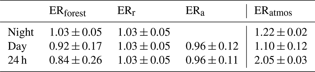
Table 3The exchange ratio for the atmosphere (ERatmos: Sect. 3.2), the forest (ERforest: Sect. 3.3), and assimilation and respiration (ERa and ERr: Sect. 3.3) for different time periods of the representative day. The time periods used to calculate the signals are the following: 09:00–13:00 for day and 23:00–04:00 for night of ERatmos and 09:00–17:00 for day and 21:00–04:00 for night of ERforest, ERr, and ERa. Note that the uncertainty for ERatmos does not represent the same uncertainty as for ERforest, since the first is the error of the fit, and the second is based on error propagation of the half-hourly measurements.
3.4 GPP and TER calculations
We found the ER signals for assimilation (ERa) and respiration (ERr) by using Eq. (9) (Fig. 7b and Table 3). The assumption that ERr stays constant throughout the day seems reasonable, because the ERforest values stay stable during the night. The ERr signal therefore becomes 1.03 ± 0.05. A more elaborate discussion of this assumption can be found in Sect. 4.5. ERa of the daytime is 0.96 ± 0.11, which indicates the ERa signal of the boreal forest when the surface fluxes are the highest. The ERa signal of the entire diurnal cycle is 0.95 ± 0.11, which also includes the assimilation processes during sunrise and sunset. Figure 7b shows all these ER signals and how they change throughout the day, together with their carbon fluxes. ERa, ERr, and the resulting ERforest signals are more realistic compared to the ERatmos signals. We will elaborate on these differences in Sects. 4.4 and 4.5.
By using Eqs. (8) and (9) for a second representative day (13 through 15 June), with the ERa and ERr signals determined from the representative day, we show in Fig. 8 that the O2 method compares well with the EC method. This means that the O2 method could potentially be used to separate NEE into GPP and TER on any day when good simultaneous CO2, O2, and NEE measurements are available. The difference between the CO2 fluxes determined with the O2 method and the EC method of both the GPP and the TER flux are around 0.5 , which is less that 6 % of the total gross flux. The difference is relatively small, which means that the O2 method compares well with the EC methods to separate NEE into GPP and TER. The different error bars in Fig. 8 show how sensitive the O2 method is to the accuracy of ERforest. By changing ERforest by 0.2, the GPP estimation by the O2 method changes by 4 , and by changing ERforest by only 0.01, the GPP estimation changes by 0.2 . The effect of changing ERforest on TER has the same effect on GPP. This shows that the O2 method is quite sensitive to ERforest and should be measured accurately, with a suggested precision of around 0.05. With a precision of 0.05 for ERforest, the GPP and TER fluxes derived with the O2 method stay in the same range as the GPP and TER fluxes determined with the EC method. The application of the O2 method will be further discussed in Sect. 4.5.

Figure 8The CO2 fluxes of a second representative day (13 through 15 June) for net ecosystem exchange (NEE), gross primary production (GPP), and total ecosystem exchange (TER) based on two different methods: the EC method and the O2 method. The different error bars indicate an increase/decrease of 0.2, 0.1, or 0.01 for the exchange ratio of the forest (ERforest) used in the O2 method.
We aimed to advance understanding of the O2:CO2 exchange ratio and its diurnal variability over a boreal forest by continuously measuring both O2 and CO2 concentrations at two heights above the canopy. These measurements gave us the possibility to compare the ERatmos and ERforest signal of an aggregate representative day and compare the boreal forest signals to previous studies in different ecosystems. Our ERatmos signal changed between the day (2.28) and the night (1.22) and had an overall diurnal signal of 2.05. For the ERforest signal, we needed to determine the O2 and CO2 surface fluxes based on the two heights. Different flux-calculating methods were compared. The O2 flux was calculated with the method that resulted in the best comparison to EC fluxes for CO2, where we found that the exchange coefficient K based on the CO2 data was most suited. The resulting ERforest signal showed again differences between the day (0.92) and night (1.04), and the overall diurnal ERforest was 0.83. For these differences and variability in the ER signals, different aspects of the uncertainty have to be taken into account, on which we elaborate in the next sections.
4.1 Measurement uncertainty
By analysing the mean difference and standard deviation of the target cylinder values between 16 June 2019 and 17 July 2019 (Table 1), we see that the values are relatively high. Previous studies that used a fuel cell analyser for continuous atmospheric O2 measurements (Battle et al., 2019; Ishidoya et al., 2013; van der Laan-Luijkx et al., 2010; Popa et al., 2010; Pickers et al., 2022) achieved measurement precision of around 5 per meg. The WMO recommends a compatibility goal of 2 per meg; however, this is difficult to achieve and so the extended compatibility goal is 10 per meg for the worldwide O2 monitoring network (Crotwell et al., 2020), which shows that our long-term measurement precision of 19 per meg is relatively poor. This poor measurement precision could have been caused by several reasons. The O2 values of the calibration cylinders that were used were relatively far apart, making it more difficult to measure the values around the target cylinder value. For 2018, we used calibration cylinders with the following values (on the SIO scale): −628.53, −816.17, and −1208.28 per meg, and for 2019 we used cylinders with values of −729.96, −816.17, and −1208.28 per meg. The cabin in which the instrument and cylinders were located was not well insulated, which created unstable temperature conditions that might have affected the stability of the cylinders (Keeling et al., 2007). The calibrations of our representative aggregate day took place during the night; therefore, large temperature changes during the day might have affected daytime stability of the reference cylinder. Furthermore, tiny leakages in the setup might have influenced the measurements. Due to the relatively short period for these campaigns and the remote location, it is not possible to trace back the cause of this large uncertainty. This high uncertainty resulted in a larger uncertainty of the vertical gradient of the two heights of the O2 measurements. However, in this study we are mostly interested in the diurnal variability of the ER signal and differences between ERatmos and ERforest; therefore, the long-term stability of the measurements are less relevant here compared to other O2 studies.
To reduce the effect of the high measurement uncertainty and derive a more statistically robust signal of the vertical gradient, we created an aggregate representative day based on days with similar weather and atmospheric conditions. The increased statistics of this representative aggregate day decrease the effect of the low measurement precision. We also move away from the reality of one specific day but rather focus on an average situation and variability of the ER signal above a boreal forest based on O2 and CO2 measurements at two levels. Given that very few previous studies focused on deriving forest ER signals globally, our analysis helps to gain further understanding of the diurnal variability and the difference between ERatmos and ERforest, which will be discussed in the following sections.
4.2 ERatmos signal in comparison to previous studies
Despite the uncertainty in our measurements, there are clear differences between the slopes of O2 and CO2 throughout the diurnal cycle (Fig. 5). Three different ERatmos signals are visible, with two signals for the day (2.28 ± 0.01 and 1.10 ± 0.12) and one for the night (1.22 ± 0.02) slope (Table 3). Note that the uncertainty of these values is based on the slope of the fitted line in Fig. 5 and does not represent the uncertainty in the stability of our measurements indicated in Table 1. The difference between day and night values of ERatmos was expected, because different processes (i.e. respiration, assimilation and entrainment) with different ER signals play a role at different times during the diurnal cycle. To exclude as much as possible the effect of entrainment and the boundary layer dynamics during the morning transition, we will from now on refer to the 1.10 value as the day ERatmos signal, which is the signal derived form period P3a. ERatmos for the complete day results in 2.05 ± 0.03.
Table 4The different exchange ratio (ER) signals of previous studies are given, with the ER of the atmosphere (ERatmos), the ER of the forest (ERforest), the ER of the respiration processes (ERr), and the ER of the assimilation processes (ERa). Bat, 2019 is short for Battle et al. (2019), Ish, 2015, represents Ishidoya et al. (2015), Ish, 2013, represents Ishidoya et al. (2013), and Sei, 2004, represents Seibt et al. (2004).
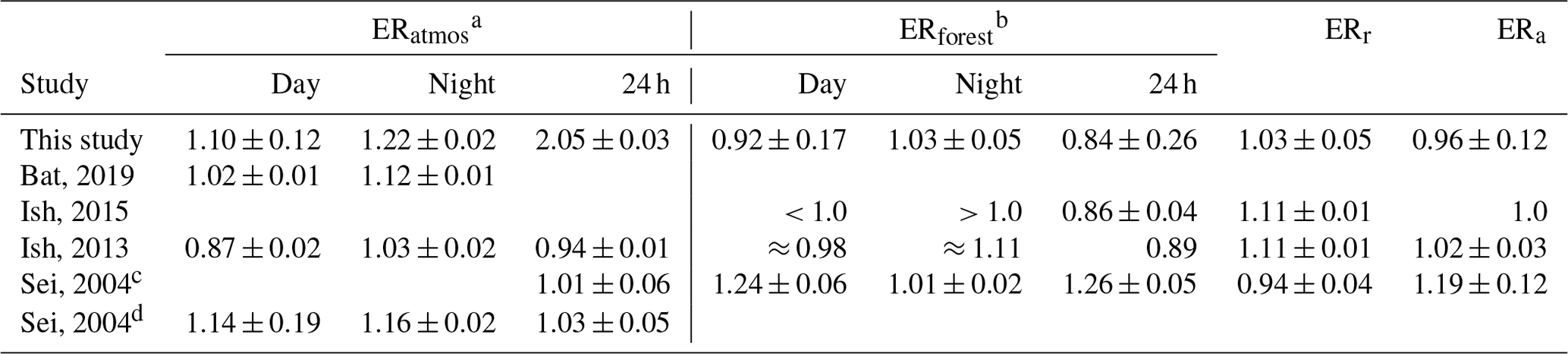
a An ER signal is classified as ERatmos when the ER signal is based on one concentration measurement of O2 and CO2. b An ER signal is classified as ERforest when the ER signal is based on surface fluxes from either a one-box model or vertical gradient flux calculations. c The ER signals of the location Griffin Forest by Seibt et al. (2004) are used here. d The ER signals of the location Harvard Forest by Seibt et al. (2004) are used here.
When comparing our ERatmos signals to those from Battle et al. (2019), Ishidoya et al. (2013), and Seibt et al. (2004) (Table 4), we note several similarities but also some differences regarding the specific values of the ERatmos signals. Our daytime signal of 1.10 is similar to 1.02, 0.87, and 1.14 from the previous studies, respectively, as is our nighttime signal of 1.22 compared to 1.12 (Battle et al., 2019), 1.03 (Ishidoya et al., 2013), and 1.16 (Seibt et al., 2004). However, our 24 h ERatmos signal of 2.05 shows an unrealistically high number which clearly does not indicate the ER of the forest only. A typical ERatmos signal for a 24 h period lies around 1, as is shown in Table 4 and by Stephens et al. (2007) and Manning (2001). Our 24 h ERatmos value includes the measurement points of the period that is influenced by entrainment and boundary layer dynamics (P2), for which period we found an ER signal of 2.28. The large influence of entrainment and boundary layer dynamics made it difficult to be very precise about the specific time periods to choose for P3. Moving the selected time boundaries of P3a from 09:00 to 09:30 or from 13:00 to 12:30 leads to ERatmos values of 0.88 or 1.75, respectively. The large changes in the daytime ERatmos due to small changes in the time boundaries show the high uncertainty of the daytime ERatmos. Therefore, our measurements provide a confirmation of earlier indications (Seibt et al., 2004) that ERatmos is an unreliable estimate for the ER of a forest, and we recommend to use ERforest.
Instead, ERatmos also represents how O2 and CO2 are influenced by the boundary layer dynamics and entrainment (Fig. 1). The high ERatmos values cannot be explained by signals from other sources, such as fossil fuel combustion or exchange with the lake, as both are not represented in the footprint of our measurements (see Sect. 2.3). Furthermore, we have shown that these high values are not an artefact from the instability of the pressure stabilization, as preliminary analysis of the ERatmos values from our 2018 measurements also show values higher than 2.0 (not shown). Although we cannot fully rule out remaining artefacts in the calibration due to, for example, temperature changes in the measurement cabin, we suggest that the more plausible explanation is that ERatmos is highly influenced by atmospheric processes, such as entrainment. The entrainment of air from either the residual layer (early in the morning transition) or the free troposphere (after the residual layer is dissolved) could impact the ERatmos as different sources of air are mixed. The residual layer contains air from the day before and could be affected by horizontal advection, whereas the air in the free troposphere originates from different background sources. These difference sources can have different ER signals and therefore create a mixture of air where O2 and CO2 are influenced differently. These air masses affect O2 differently compared to CO2 in the boundary layer, and an ERatmos signal will arise that cannot be linked directly to one specific process. Even though entrainment processes also occur at locations of previous studies, we still find differences in ERatmos. We suggest that this can be explained by difference in measurement height compared to the canopy height and different sources of background air in the free troposphere at the measurement location. For the ERatmos signal during P2 at 125 m, we find a value of 3.40, even higher than the ERatmos signal of 2.28 at 23 m, which indicates that the influence of entrainment increases when measuring further away from the canopy, and as a result the ERatmos signals show higher values. Further insights into the contributions of each process to ERatmos cannot be estimated from the measurements alone and would require using an atmospheric model.
4.3 Uncertainties in the CO2 and O2 flux calculations
By comparing the theoretical and observation-based methods, we determined that the most suitable method to calculate both the CO2 and O2 fluxes was to use the observation-based method with CO2 data (Sect. 3.3). Figure 6 and Table 2 show that the theoretical methods (MOST and integrated) resulted in a change of the CO2 flux that was late compared to the EC measurement. This delay has been described before and is caused by the time it takes before the turbulence can mix the CO2 gradient driven by stable nocturnal stratification conditions and establish the corresponding gradient to how turbulent the atmosphere is (Casso-Torralba et al., 2008). When the heights of the gradient are closer together, the delay is less pronounced. However, the measurement heights used during our campaign are relatively far apart (125 m and 23 m), and the EC flux is measured at 27 m. The 125 m measurement is even located outside the surface layer during the morning transition. This made the flux-gradient method (as described in Eq. 7) less applicable, which assumes that the surface flux stays constant in the surface layer (Dyer, 1974).
Since during our campaign we only measured at two heights, we missed information on the logarithmic profile originating from the canopy top, which resulted in an underestimation of the flux using the K with MOST method. This was solved by integrating the MOST equation (integrated method). With the integrated method, the gradient is assumed to be logarithmic, and the total flux increases compared to the MOST calculation (Paulson, 1970). However, with the large difference between the two measurement heights, the integrated approach still overestimated the CO2 flux compared to the EC measurements during both the day and the night. Also, the delay in the timing of the sign change of the gradient cannot be solved with this integrated method. We also explored the effect of adding a roughness surface layer (RSL) in the flux calculations of the theoretical methods, by adding an extra factor that accounts for this layer (not shown in the results) (de Ridder, 2010). The contribution of the RSL did not improve our results, because it also includes the delay of the gradient which was causing the largest deviation in the theoretical methods (Table 2).
By applying both observation-based methods, using either θ or CO2 to infer the exchange coefficient K, we did not find this delay in the timing of the gradient, and the observation-based methods therefore resulted in derived fluxes close to the EC measurements. Here it has to be noted that the ICOS EC measurements of CO2 that we used as a benchmark for the most suitable flux calculation approach were also used in calculating K with CO2, which makes the comparison of these approaches to the CO2 flux not fully independent. Note that we first derive K with the vertical CO2 gradients calculated from ICOS CO2 observations at three vertical levels, and we apply this to our own measurements of the CO2 vertical gradient with an independent instrument (Table B1). As a result, there is not a full circularity when comparing the obtained fluxes to the EC CO2 measurements to select which method for calculating K we use. Most previous studies that determined fluxes based on the gradient approach used θ to calculate K (Stull, 1988; Mayer et al., 2011; Wolf et al., 2008; Bolinius et al., 2016; Brown et al., 2020), because θ is the driver of convective turbulence. However, because O2 is directly linked to CO2 and because our statistics (Table 2) indicated that the CO2 method resulted in a better comparison to the EC fluxes, we decided to use the ICOS CO2 data at three levels and the CO2 EC measurements to calculate K. This K together with the measurements of two heights by our instrument during our campaign were used to calculate both the CO2 and the O2 fluxes used in our study. We also tested the impact of using only two vertical levels of the ICOS CO2 concentrations to calculate K (not shown), which was also the case in the only previous study that derived O2 fluxes. Ishidoya et al. (2015) derived O2 fluxes for a temperate forest in Japan using two vertical levels at 18 and 27 m height for both O2 and CO2 concentrations. Our comparison of deriving K based on two vertical levels (23 m and 125 m) resulted in an underestimation of the gradient and thus an overestimation of K, and as a consequence the calculated CO2 flux was overestimated. Therefore, the three levels of ICOS CO2 concentration measurements proved to be vital in our flux calculations here. We still missed the logarithmic profile at the surface with only the two vertical campaign measurements, and as a result we slightly underestimated the final CO2 and O2 flux. Therefore, we recommend to always measure at least three heights of CO2 and O2 inside the surface layer when they are meant to be used for flux calculations.
Our final O2 flux (Fig. 6) shows a clear diurnal cycle, with the expected behaviour of negative values in the night (O2 consumption for respiration) and a positive flux during the day (O2 release during assimilation). The nighttime fluxes are more stable and give a clear signal due to the larger vertical gradient. K is more difficult to determine during the night as the EC measurements are less representative due to the low level of turbulence. However, the largest contributor to the uncertainty is our own O2 measurements, and the larger gradient allows us to better establish the O2 flux. The larger variability of the daytime O2 fluxes is caused by the smaller gradient of the O2 concentration measurements during the day (Fig. 3), when the atmosphere is more well mixed and when the difference between the two heights becomes smaller. The relatively large measurement uncertainty made it difficult to measure these small differences between the two heights and increased the noise in the fluxes. The measurement noise resulted in O2 gradient variations that were not tied to the CO2 gradient variations, and this degraded the correlation between the two fluxes. Despite this larger variability, we still find a clear diurnal behaviour, which allowed us to calculate ERforest. Note that the uncertainties of the surface fluxes of O2 and CO2 are only based on the measurements from our campaigns, and we did not include the uncertainties that are related to the calculations of K based on the ICOS data. However, the uncertainty in K is relatively small compared to the other terms in the calculation, and the final uncertainty of estimates is dominated by the measurement uncertainty of O2. Omitting the uncertainty associated with K therefore leads to a minor underestimate of the full uncertainty.
4.4 ERforest signal compared to previous studies
Our resulting ERforest signal changes throughout the diurnal cycle, with specific daytime (0.92 ± 0.17), nighttime (1.03 ± 0.05), and overall (0.84 ± 0.26) values (Fig. 7 and Table 3). The individual nighttime values show a smaller uncertainty due to the already explained effect of the larger gradient during the stable atmospheric conditions of the night. In contrast, the individual daytime values show a larger uncertainty due to the smaller gradient during the unstable atmospheric conditions of the day. We therefore used averaged values for the daytime and nighttime signals to derive the ERforest values. While the daytime signal excludes the entrainment and the boundary layer dynamics during the morning transition, these effects are still included in the overall ERforest signal. Note that the overall 24 h signal is not the average of the daytime and nighttime signal. The nighttime ERforest signal represents a negative O2 flux and a positive CO2 flux, whereas the daytime ERforest signal represents a positive O2 flux and a negative CO2 flux. This means that the daytime and nighttime surface fluxes influence the atmosphere differently; therefore, these ERforest values cannot be averaged to calculate the overall ERforest signal. By first calculating the average overall O2 and CO2 fluxes and then dividing these, we derive the overall ERforest signal correctly.
When comparing our ERforest signals to previous studies by Seibt et al. (2004), Ishidoya et al. (2013), and Ishidoya et al. (2015) (Table 4), we notice that the difference between the daytime and the nighttime values that we found and the specific values of the different ERforest has some similarities and some differences. Our results, along with those by Ishidoya et al. (2013, 2015) (night: 1.11 and day: 0.98), show that the ERforest signal of the nighttime is higher than the daytime signal, whereas Seibt et al. (2004) (day: 1.24 and night: 1.01) show the opposite behaviour. Our results are most similar to the signals of both Ishidoya et al. (2013) and Ishidoya et al. (2015), especially if we take our uncertainty range into account. The 24 h signals are difficult to compare as we used a different method to determine the overall ERforest signal compared to Ishidoya et al. (2015). In this study we use average fluxes instead of a linear regression through either the O2 and CO2 fluxes or vertical gradient, and we thereby take into account the size of the fluxes that contributes most to the ER signal, which results in a flux-weighted average ERforest. We note again that we need to distinguish between daytime and nighttime signals, and we cannot just average them. Figure 7 illustrates the need to take averages in consistent meteorological and biological periods that are characterized by similar turbulence regimes and similar signs of the O2 and CO2 exchange. For example, combining a small negative O2 flux with a high ER with a large positive O2 flux with a lower ER results in a smaller O2 flux compared to when the ERs of both fluxes would have been the same. When we take into account our uncertainty, the complete day signal of 0.84 ± 0.26 comes close to the globally used average ER of the biosphere of 1.1 (Severinghaus, 1995). However, the specific value suggests that the overall ERforest signal of this boreal forest lies somewhat lower than 1.1, i.e. closer to 1.0. The difference in ERforest signals between studies can be explained with the different ERa and ERr signals, which we discuss in Sect. 4.5.
The ERforest and ERatmos signals are not identical; therefore, they do not represent the same information (Table 3). The ERatmos signals are higher compared to the ERforest signals; the 24 h signals especially show a large difference. Despite the higher numbers, the day and night signals of ERatmos and ERforest both show the same pattern, where the daytime signal is lower compared to the nighttime signal. When comparing these differences to previous studies, we find that not all studies find the same results. The difference between ERforest and ERatmos was not found by Ishidoya et al. (2013). In contrast, Seibt et al. (2004) found a difference between ERforest and ERatmos (Table 4). A reason for this could be the measurement height of ERatmos. When ERatmos is determined closer to the canopy and inside the roughness sublayer, it will be more influenced by the surface processes compared to measurements at higher levels, which are seeing more integrated signals of all processes that influence the concentrations inside the atmospheric boundary layer (i.e. forest exchange and non-local processes like entrainment). To get a clear answer to this question, we should further investigate to what extent ERatmos is influenced by entrainment and boundary layer dynamics and under which conditions they can come close to ERforest. We already show that excluding the morning transition (P2) helps to improve the ERatmos signal. However, as already stated, it is difficult from the measurements alone to determine if the ERatmos signal is influenced only by the surface during this period. An atmospheric model would therefore be needed to find how ERatmos can be derived from a single measurement height and to allow for comparison with previous studies that measured at one height to determine the ER of the forest (Battle et al., 2019; van der Laan et al., 2014; Stephens et al., 2007). We are currently applying a specific mixed-layer atmospheric model to further investigate this.
4.5 The ERa and ERr signals
To further understand the relationship between O2 and CO2, we cannot use the ERforest signal alone. To look in more detail into the processes driving the variations, we calculated the exchange ratios of respiration (ERr) and assimilation (ERa) (Table 3 and Fig. 7). ERr was taken as the ERforest nighttime signal (1.03 ± 0.05), by assuming that only respiration influences the ERforest signal during the night and that the ERr signal stays constant throughout the entire day. This means that both the heterotrophic and autotrophic respiration are included in ERr, and the same components are respired in the same ratios throughout the day to keep ERr a constant value. The studies that looked at the ERr of an ecosystem (Hilman et al., 2022; Angert et al., 2015; Hicks Pries et al., 2020) only focused on longer timescales than the diurnal cycle. It is therefore not possible to derive diurnal variability of ERr from these previous studies. We would expect some changes in ERr as temperatures change during the day, and the respiration of plants involves photorespiration during daytime and dark respiration during nighttime. However, as the study by Hilman et al. (2022) showed, the variability of ERr mainly depends on the bulk soil respiration and therefore depends on the soil temperature and soil moisture. No large changes in temperatures or soil moisture were detected during the period of the representative aggregate day; therefore, it is unlikely that the ERr significantly changed in that period. To get a more detailed view on how the ERr of an ecosystem changes throughout the day, more research is needed on the variability of ERr including from plant respiration by chamber measurements.
The variability of ERr between locations highly depends on the soil properties (Angert et al., 2015), which makes it difficult to compare with the few studies available (Seibt et al., 2004; Ishidoya et al., 2013) that measured ERr with chamber measurements on a brown soil. The soil in our study area is a podzol, which is characterized by a high acidity with little organic matter (Buurman and Jongmans, 2005). The OR of podzols is around 1.08 (Worrall et al., 2013), and the ER of acid soils is expected to be around this OR, because carbon cannot easily dissolve into the groundwater (Angert et al., 2015), and we therefore conclude that our ERr value of 1.04 is realistic.
We looked at two options to calculate ERa: the ERa based only on the daytime measurements (between 09:00 and 17:00: 0.96 ± 0.12) and ERa based on all the measurements (throughout the 24 h period: 0.96 ± 0.11). Both numbers are close to 1, which is often assumed as a standard value for ERa (Ishidoya et al., 2015; Severinghaus, 1995). Next to that, a value of ERa close to 1 means that ammonium is used as a source for nitrogen instead of nitrate (Bloom et al., 1989, 2012). Ammonium is indeed a larger source for nitrogen compared to nitrate in Hyytiälä (Korhonen et al., 2013). The OR of needle leaves (and plant material in general) appears to be always close to 1.0 (Jürgensen et al., 2021), which again confirms our ERa signals. We did not observe differences between the two ERa signals. The transition periods between the night and the daytime were difficult to measure, because the gradient then becomes close to zero, which means there could be a possibility that next to ERforest, ERa also has a diurnal cycle. Again, there are only a few studies that looked at the variability of ERa (Fischer et al., 2015; Bloom et al., 1989, 2012; Bloom, 2015). The available studies show that ERa depends on light (Fischer et al., 2015) and the source of nitrogen in the soil (Bloom, 2015). These changes in ERa happen when the changes in the atmosphere and the soil are sudden and persist for a longer time compared to a diurnal cycle. We can therefore say that the ERa also does not change drastically during the day. To get a more detailed overview of ERa, more precise measurements are needed with uncertainties lower than 0.1 for the ER signals. However, the similar values of ERa that we find for the daytime and 24 h measurements show that ERa is hardly affected by entrainment during the morning transition, and it would suggest that the morning transition is less of an issue for ERforest than for ERatmos.
By applying the O2 method to a new aggregate day, we showed that the O2 method gives results similar to the EC method to partition NEE and derive the GPP and TER fluxes (Fig. 8), with estimates of the uncertainties of the O2 method. The EC method also contains uncertainties in its approach because of the reliance on a function of temperature and should therefore not necessarily be assumed to be the truth (Reichstein et al., 2005). Despite the uncertainty of both the O2 method and the EC method, both methods give similar results for the CO2 flux of GPP and TER. In our comparison of the O2 and EC methods, there is a minor degree of circularity, as we use the EC GPP estimates to estimate ERa. By applying it to another representative day, we prevent a full circularity (Table B1). In this campaign, we unfortunately could not determine the ERa and ERr signals independently from EC, which would be recommended for a full comparison. This would have been possible by using chamber measurements. We expect only minor changes in ERa from branch/leaf chamber measurements compared to the values we derived, because our ERa is in the range of expected values compared to previous studies (e.g. Jürgensen et al., 2021; Bloom, 2015; Fischer et al., 2015). The satisfactory comparison between the O2 and the EC methods for the partitioning of the fluxes shows the potential of the O2 method. The largest challenge for this method is to determine ERforest with large enough accuracy, as this value is most variable and most difficult to determine based on the small O2 gradients that we observed. Figure 8 shows that the ERforest signal should be measured with an uncertainty of 0.05 or less to get results within the uncertainty range of the EC method. When such high accuracy is reached, the O2 method has the potential to provide an alternative method for the separation of GPP and TER without relying on the regularly used temperature-based function as used for the EC method. Ishidoya et al. (2015) showed similar results, where the O2 method also produced GPP and TER comparable to the EC method and the magnitude of the GPP and TER fluxes highly dependent on the derived ERa and ERr signals.
To allow for an independent comparison between the flux partitioning with the EC method and the O2 method, such as was done by using δ13CO2 by Wehr et al. (2016), we recommend measuring the ERr and ERa signals directly with chamber measurements (Seibt et al., 2004; Ishidoya et al., 2013). We also recommend to add at least one additional measurement height for the O2 and CO2 concentrations below the canopy to apply the storage correction for both the O2 and the CO2 fluxes (Aubinet et al., 2012) and to add a measurement in the free troposphere to better evaluate the effect of entrainment. Despite the high dependency on the accuracy of the ER, this study showed again, as did Ishidoya et al. (2015), that the O2 method can be used to get a better understanding of the carbon cycle. To further develop this method, we need to expand the O2 measurements for longer time series and more locations and to analyse how ERforest varies over longer timescales, which can improve the global average value of ER (αB) of 1.1 as used in global carbon budget studies such as Manning and Keeling (2006).
By continuously measuring atmospheric O2 and CO2 concentrations at two heights in Hyytiälä, Finland, we gained new insights into the diurnal variability of O2 and CO2 above a boreal forest, quantified by interpreting their exchange ratio (ER). We showed that the signal based on one measurement height of the O2 and CO2 concentrations (ERatmos) is not representative for the exchange between the forest and the atmosphere only, but it instead includes other processes such as entrainment as well. To derive the ER of the forest specifically (ERforest), we first determined the surface fluxes above the canopy of O2 and CO2 using the vertical gradient between the two measurement heights. We found that the most suitable method to calculate both the O2 and CO2 surface fluxes was to use the exchange coefficient calculated from the eddy covariance (EC) CO2 flux and the vertical gradient of CO2 measurements at three heights above the canopy. The ERforest signals that resulted from the ratio of the mean O2 and CO2 fluxes varied between the daytime (0.92 ± 0.17 mol mol−1) and nighttime (1.03 ± 0.05 mol mol−1). The different ERforest signals were composed of the ER of respiration (ERr: 1.03 ± 0.05 mol mol−1) and the ER of assimilation (ERa: 0.96 ± 0.12 mol mol−1). With these findings, we show improved methods to derive O2 forest fluxes and to derive the variability in the different ER signals over a representative diurnal cycle. The ERforest signal shows a clear diurnal cycle for this boreal forest, and the overall ratio is lower than 1.1 that is used in global carbon budget calculations. Finally, we show that these ER signals can be used to separate net ecosystem exchange (NEE) into gross primary production (GPP) and total ecosystem respiration (TER).
With only a few data sets of continuous measurements of both O2 and CO2 concentrations over forests, our data set is of high importance, specifically the availability of measurements at two heights that allow for calculation of O2 and CO2 fluxes. Our analyses can serve as a starting point for follow-up research using coupled land surface–atmosphere models to distinguish and quantify contributions of different processes to ERatmos and ERforest signals. Further understanding of these differences will help to fully exploit the advantages of atmospheric O2 when unravelling the different components in the carbon cycle.
A1 Observation-based method
The gradient between three points is calculated with the following equation:
where z [m] is the height above the displacement height (d [m]) (d is taken as canopy height); is the average variable where the line is fitted through; and a, b, and c are the resulting fitted parameters. When only two vertical measurements are available, the gradient was determined using finite differences.
A2 Theoretical approach
For the MOST method, the following equations were used (Physick and Garratt, 1995):
where K is the exchange coefficient [m2 s−1], κ = 0.4 is the von Kármán constant, u∗ [m s−1] is the friction velocity, ΦH [–] indicates the stability function, and ϕrsl [–] indicates the contribution of the roughness sublayer (RSL). The ΦH was calculated with the following (Dyer, 1974):
where L [m] is the Obukov length, which was based on the following equation (Dyer, 1974):
where θv [K] is the virtual potential temperature, [K m s−1] is the virtual surface heat flux, and g [m s−2] is the acceleration due to gravity. Because the flux was measured close to the canopy, the roughness surface layer (RSL) could become important. The RSL needs an additional length scale (ϕ) and can be calculated with the following equation (de Ridder, 2010):
Here z∗ [m] indicates the height of the RSL above the displacement height and we take that as (2 ⋅ canopy height − d), and μ is a constant of 0.95 [–].
By integrating Eq. (7) with Eq. (A3) for K, we get the following equation that was used for the integrated method (Physick and Garratt, 1995):
where ΨH [–] represents the integrated stability functions for heat, and ψ [–] is the integrated function to account for the roughness sublayer (RSL) effect. ΨH was calculated with (Paulson, 1970)
The function of the integrated RSL length scale (ψRSL) [–] was calculated with (de Ridder, 2010)
where ν and λ are both parameters, taken as 0.5 and 1.5, respectively.
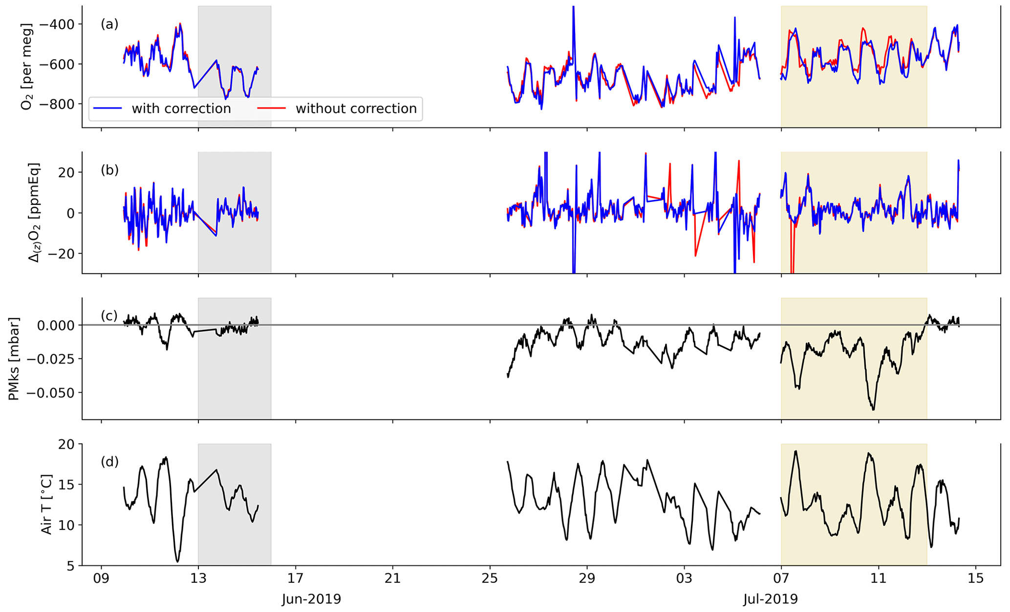
Figure B1The corrected and uncorrected half-hourly average O2 concentrations at 23 m for the PMKS deviations (a), together with the corrected and uncorrected gradient of O2 (b). The time series for the 2019 measurement period of the PMKS (c) and the air temperature (d) are also shown. The shaded areas indicate the dates that were selected for the two aggregate representative days, i.e. 13 through 15 June (grey) and 7 through 12 July 2019 (yellow).
Table B1Here are the data used to calculate different variables that we calculated in our study for the two aggregate days. Part (a) indicates the data that were used for the first representative aggregate day during 7 through 13 July 2019, and part (b) indicates the data that were used for the second aggregate day between 13 and 15 June 2019. The data used are mostly from the period of the respective aggregate day, except when indicated otherwise.
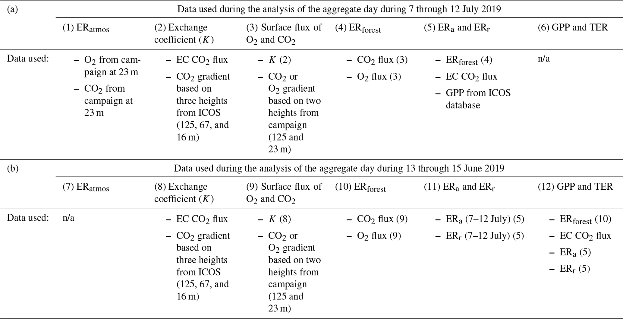
n/a = not applicable
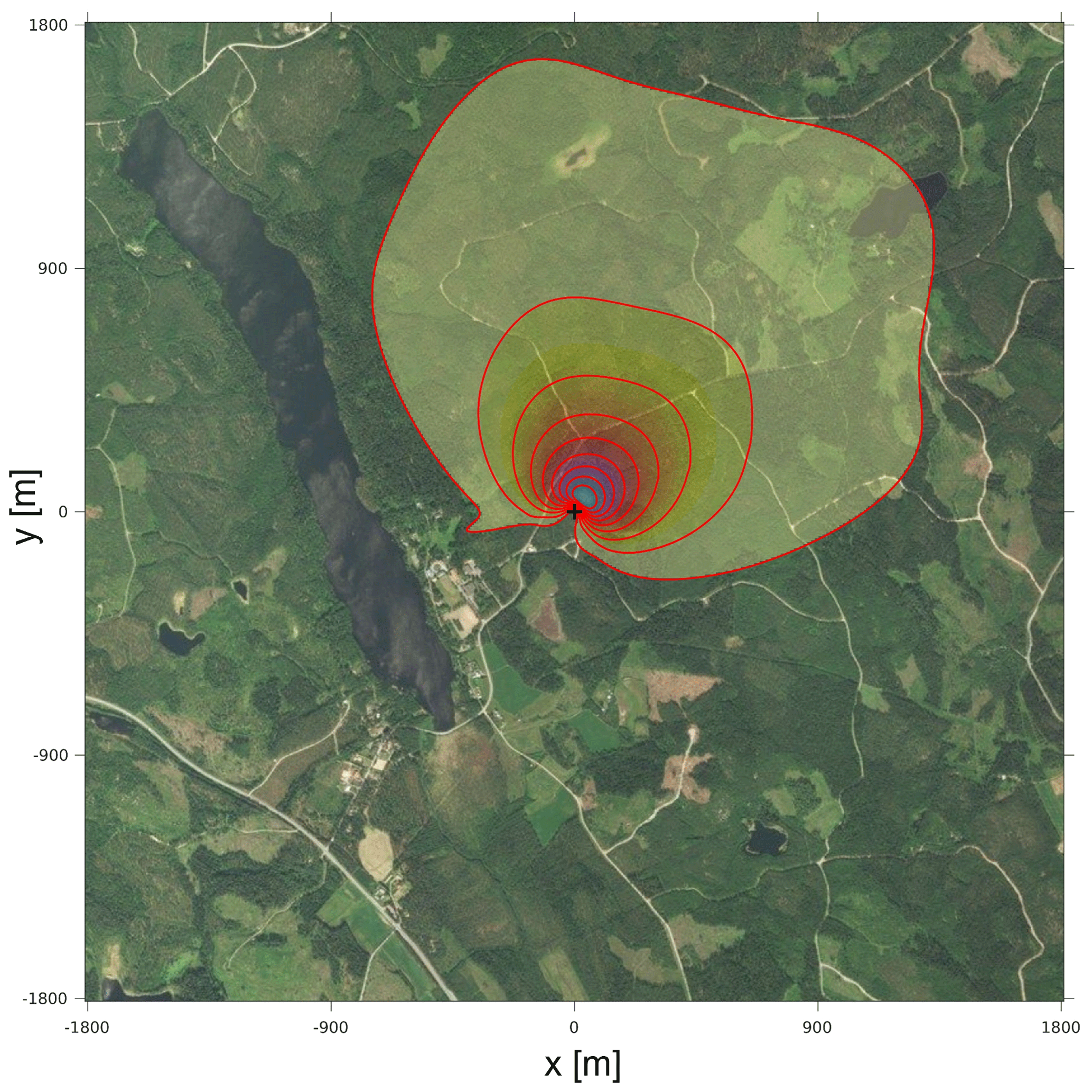
Figure B2The footprint of the O2 and CO2 surface fluxes at 53.6 m height (which is the geometric height), determined with the gradient method for the days during 7 through 12 July 2019 at Hyytiälä. The lines and contours indicate the contributions to the footprint from 10 % to 90 % in steps of 10 %. The plus sign (+) indicates the location of the tower. This figure was created with the method by Kljun et al. (2015).
The data used in this study are available from https://doi.org/10.18160/SJ3J-PD38 (Faassen and Luijkx, 2022).
ITL designed the measurement campaign and conducted the measurements. ITL, ERB, LNTN, PAP, and ACM contributed to the design and development of the O2 and CO2 measurement setup. LNTN, BAMK, IM, and TV contributed to the measurement campaigns. KAPF and ITL analysed the measurements. KAPF, ITL, WP, JV, and HAJM interpreted and discussed the methods and results. KAPF and ITL wrote the paper with input from all co-authors.
The contact author has declared that none of the authors has any competing interests.
Publisher's note: Copernicus Publications remains neutral with regard to jurisdictional claims in published maps and institutional affiliations.
The authors would like to thank Janne Levula (previously worked at Institute for Atmospheric and Earth System Research (INAR)/Physics, Faculty of Science, University of Helsinki, Helsinki, Finland) and Bert Heusinkveld (Meteorology and Air Quality, Wageningen University and Research, Wageningen, the Netherlands) for their help at Hyytiälä during the measurement campaigns, Marcel de Vries (Centre for Isotope Research (CIO), Energy and Sustainability Research Institute Groningen, University of Groningen, Groningen, the Netherlands) for technical support, and Charlotte van Leeuwen (previously at Centre for Isotope Research (CIO), Energy and Sustainability Research Institute Groningen, University of Groningen, Groningen, the Netherlands) for the development of the instrument. This work was supported with funding that ITL received from the Netherlands Organisation for Scientific Research (016.Veni.171.095). We thank Üllar Rannik and Pasi Kolari (Institute for Atmospheric and Earth System Research (INAR)/Physics, Faculty of Science, University of Helsinki, Helsinki, Finland) for their work on the interpretation and analysis of the Hyytiälä flux measurements and their footprint. We thank the three anonymous reviewers for their comments which helped to improve this paper.
This research has been supported by the Nederlandse Organisatie voor Wetenschappelijk Onderzoek (grant no. 016.Veni.171.095).
This paper was edited by Andreas Hofzumahaus and reviewed by three anonymous referees.
Angert, A., Yakir, D., Rodeghiero, M., Preisler, Y., Davidson, E. A., and Weiner, T.: Using O2 to study the relationships between soil CO2 efflux and soil respiration, Biogeosciences, 12, 2089–2099, https://doi.org/10.5194/bg-12-2089-2015, 2015. a, b, c, d
Aubinet, M., Vesala, T., and Papale, D.: Eddy covariance: a practical guide to measurement and data analysis, Springer Science & Business Media, Springer Dordrecht, The Netherlands, https://doi.org/10.1007/978-94-007-2351-1, 2012. a
Ballantyne, A. P., Alden, C. B., Miller, J. B., Tans, P. P., and White, J. W. C.: Increase in observed net carbon dioxide uptake by land and oceans during the past 50 years, Nature, 488, 70–72, 2012. a
Battle, M. O., Munger, J. W., Conley, M., Sofen, E., Perry, R., Hart, R., Davis, Z., Scheckman, J., Woogerd, J., Graeter, K., Seekins, S., David, S., and Carpenter, J.: Atmospheric measurements of the terrestrial O2:CO2 exchange ratio of a midlatitude forest, Atmos. Chem. Phys., 19, 8687–8701, https://doi.org/10.5194/acp-19-8687-2019, 2019. a, b, c, d, e, f, g, h, i, j
Blaine, T. W., Keeling, R. F., and Paplawsky, W. J.: An improved inlet for precisely measuring the atmospheric ratio, Atmos. Chem. Phys., 6, 1181–1184, https://doi.org/10.5194/acp-6-1181-2006, 2006. a
Bloom, A. J.: Photorespiration and nitrate assimilation: a major intersection between plant carbon and nitrogen, Photosynth. Res., 123, 117–128, 2015. a, b, c, d
Bloom, A. J., Caldwell, R. M., Finazzo, J., Warner, R. L., and Weissbart, J.: Oxygen and Carbon Dioxide Fluxes from Barley Shoots Depend on Nitrate Assimilation, Plant Physiol., 91, 352–356, https://doi.org/10.1104/pp.91.1.352, 1989. a, b
Bloom, A. J., Rubio Asensio, J. S., Randall, L., Rachmilevitch, S., Cousins, A. B., and Carlisle, E. A.: CO2 enrichment inhibits shoot nitrate assimilation in C3 but not C4 plants and slows growth under nitrate in C3 plants, Ecology, 93, 355–367, https://doi.org/10.1890/11-0485.1, 2012. a, b
Bolinius, D. J., Jahnke, A., and MacLeod, M.: Comparison of eddy covariance and modified Bowen ratio methods for measuring gas fluxes and implications for measuring fluxes of persistent organic pollutants, Atmos. Chem. Phys., 16, 5315–5322, https://doi.org/10.5194/acp-16-5315-2016, 2016. a
Brown, J., Shapkalijevski, M., Krol, M., Karl, T., Ouwersloot, H., Moene, A., Patton, E., and Vilà-Guerau de Arellano, J.: Ozone exchange within and above an irrigated Californian orchard, Tellus B, 72, 1–17, 2020. a
Buurman, P. and Jongmans, A.: Podzolisation and soil organic matter dynamics, Geoderma, 125, 71–83, 2005. a
Carbon Portal ICOS RI: STILT station characterization for Hyytiälä at 17 m, carbon portal, https://hdl.handle.net/11676/sbjAXeKbI09FqHDtFNqf6oVc (last access: 6 January 2023), 2022. a, b
Casso-Torralba, P., de Arellano, J. V. G., Bosveld, F., Soler, M. R., Vermeulen, A., Werner, C., and Moors, E.: Diurnal and vertical variability of the sensible heat and carbon dioxide budgets in the atmospheric surface layer, J. Geophys. Res. Atmos., 113, D12119, https://doi.org/10.1029/2007JD009583, 2008. a
Cox, P. M., Pearson, D., Booth, B. B., Friedlingstein, P., Huntingford, C., Jones, C. D., and Luke, C. M.: Sensitivity of tropical carbon to climate change constrained by carbon dioxide variability, Nature, 494, 341–344, 2013. a
Crotwell, A., Lee, H., and Steinbacher, M.: 20th WMO/IAEA Meeting on Carbon Dioxide, Other Greenhouse Gases and Related Measurement Techniques (GGMT-2019), Tech. Rep. 255, Jeju Island, South Korea, 2–5 September 2019, 2020. a
de Ridder, K.: Bulk transfer relations for the roughness sublayer, Bound.-Lay. Meteorol., 134, 257–267, https://doi.org/10.1007/s10546-009-9450-y, 2010. a, b, c, d
Dyer, A.: A review of flux-profile relationships, Bound.-Lay. Meteorol., 7, 363–372, 1974. a, b, c, d, e
Faassen, K. and Luijkx, I.: Atmospheric O2 and CO2 measurements at Hyytiälä, Finland, ICOS ERIC – Carbon Portal [data set], https://doi.org/10.18160/SJ3J-PD38, 2022. a
Fischer, S., Hanf, S., Frosch, T., Gleixner, G., Popp, J., Trumbore, S., and Hartmann, H.: Pinus sylvestris switches respiration substrates under shading but not during drought, New Phytol., 207, 542–550, 2015. a, b, c, d
Friedlingstein, P., Jones, M. W., O'Sullivan, M., Andrew, R. M., Bakker, D. C. E., Hauck, J., Le Quéré, C., Peters, G. P., Peters, W., Pongratz, J., Sitch, S., Canadell, J. G., Ciais, P., Jackson, R. B., Alin, S. R., Anthoni, P., Bates, N. R., Becker, M., Bellouin, N., Bopp, L., Chau, T. T. T., Chevallier, F., Chini, L. P., Cronin, M., Currie, K. I., Decharme, B., Djeutchouang, L. M., Dou, X., Evans, W., Feely, R. A., Feng, L., Gasser, T., Gilfillan, D., Gkritzalis, T., Grassi, G., Gregor, L., Gruber, N., Gürses, Ö., Harris, I., Houghton, R. A., Hurtt, G. C., Iida, Y., Ilyina, T., Luijkx, I. T., Jain, A., Jones, S. D., Kato, E., Kennedy, D., Klein Goldewijk, K., Knauer, J., Korsbakken, J. I., Körtzinger, A., Landschützer, P., Lauvset, S. K., Lefèvre, N., Lienert, S., Liu, J., Marland, G., McGuire, P. C., Melton, J. R., Munro, D. R., Nabel, J. E. M. S., Nakaoka, S.-I., Niwa, Y., Ono, T., Pierrot, D., Poulter, B., Rehder, G., Resplandy, L., Robertson, E., Rödenbeck, C., Rosan, T. M., Schwinger, J., Schwingshackl, C., Séférian, R., Sutton, A. J., Sweeney, C., Tanhua, T., Tans, P. P., Tian, H., Tilbrook, B., Tubiello, F., van der Werf, G. R., Vuichard, N., Wada, C., Wanninkhof, R., Watson, A. J., Willis, D., Wiltshire, A. J., Yuan, W., Yue, C., Yue, X., Zaehle, S., and Zeng, J.: Global Carbon Budget 2021, Earth Syst. Sci. Data, 14, 1917–2005, https://doi.org/10.5194/essd-14-1917-2022, 2022. a
Gallagher, M. E., Liljestrand, F. L., Hockaday, W. C., and Masiello, C. A.: Plant species, not climate, controls aboveground biomass O2:CO2 exchange ratios in deciduous and coniferous ecosystems, J. Geophys. Res.-Biogeo., 122, 2314–2324, https://doi.org/10.1002/2017JG003847, 2017. a
Hari, P., Nikinmaa, E., Pohja, T., Siivola, E., Bäck, J., Vesala, T., and Kulmala, M.: Station for measuring ecosystem-atmosphere relations: SMEAR, in: Physical and physiological forest ecology, edited by: Hari, P., Heliövaara, K., and Kulmala, L., pp. 471–487, 2013. a
Hicks Pries, C., Angert, A., Castanha, C., Hilman, B., and Torn, M. S.: Using respiration quotients to track changing sources of soil respiration seasonally and with experimental warming, Biogeosciences, 17, 3045–3055, https://doi.org/10.5194/bg-17-3045-2020, 2020. a
Hilman, B., Weiner, T., Haran, T., Masiello, C. A., Gao, X., and Angert, A.: The apparent respiratory quotient of soils and tree stems and the processes that control it, J. Geophys. Res.-Biogeo., 127, e2021JG006676, https://doi.org/10.1029/2021JG006676, 2022. a, b, c, d
Ishidoya, S., Murayama, S., Takamura, C., Kondo, H., Saigusa, N., Goto, D., Morimoto, S., Aoki, N., Aoki, S., and Nakazawa, T.: O2:CO2 exchange ratios observed in a cool temperate deciduous forest ecosystem of central Japan, Tellus B, 65, 21120, https://doi.org/10.3402/tellusb.v65i0.21120, 2013. a, b, c, d, e, f, g, h, i, j, k, l, m
Ishidoya, S., Murayama, S., Kondo, H., Saigusa, N., Kishimoto-Mo, A. W., and Yamamoto, S.: Observation of O2:CO2 exchange ratio for net turbulent fluxes and its application to forest carbon cycles, Ecol. Res., 30, 225–234, https://doi.org/10.1007/s11284-014-1241-3, 2015. a, b, c, d, e, f, g, h, i, j, k, l, m, n, o, p, q, r, s, t, u
Jürgensen, J., Muhr, J., and Knohl, A.: Variations of the Oxidative Ratio across Ecosystem Components and Seasons in a Managed Temperate Beech Forest (Leinefelde, Germany), Forests, 12, 1693, https://doi.org/10.3390/f12121693, 2021. a, b
Keeling, R.: Development of an Interferometric Oxygen Analyzer for Precise Measurement of the Atmospheric O2 Mole Fraction., PhD thesis, Harvard University, Cambridge, Massachusetts, U.S.A., 1988. a
Keeling, R., Najjar, R., Bender, M., and Tans, P.: What atmospheric oxygen measurements can tell us about the global carbon-cycle, Global Biogeochem. Cy., 7, 37–67, https://doi.org/10.1029/92GB02733, 1993. a
Keeling, R. F. and Manning, A. C.: Studies of Recent Changes in Atmospheric O2 Content, vol. 5, 2 edn., Elsevier Ltd., Treatise on Geochemistry (Second Edition), https://doi.org/10.1016/B978-0-08-095975-7.00420-4, 2014. a, b, c, d
Keeling, R. F., Manning, A. C., McEvoy, E. M., and Shertz, S. R.: Methods for measuring changes in atmospheric O2 concentration and their application in southern hemisphere air, J. Geophys. Res.-Atmos., 103, 3381–3397, 1998. a
Keeling, R. F., Manning, A. C., Paplawsky, W. J., and Cox, A. C.: On the long-term stability of reference gases for atmospheric and CO2 measurements, Tellus B, 59, 3–14, https://doi.org/10.1111/j.1600-0889.2006.00196.x, 2007. a
Kljun, N., Calanca, P., Rotach, M. W., and Schmid, H. P.: A simple two-dimensional parameterisation for Flux Footprint Prediction (FFP), Geosci. Model Dev., 8, 3695–3713, https://doi.org/10.5194/gmd-8-3695-2015, 2015. a, b
Kohonen, K.-M., Dewar, R., Tramontana, G., Mauranen, A., Kolari, P., Kooijmans, L. M. J., Papale, D., Vesala, T., and Mammarella, I.: Intercomparison of methods to estimate gross primary production based on CO2 and COS flux measurements, Biogeosciences, 19, 4067–4088, https://doi.org/10.5194/bg-19-4067-2022, 2022. a
Kooijmans, L. M. J., Cho, A., Ma, J., Kaushik, A., Haynes, K. D., Baker, I., Luijkx, I. T., Groenink, M., Peters, W., Miller, J. B., Berry, J. A., Ogée, J., Meredith, L. K., Sun, W., Kohonen, K.-M., Vesala, T., Mammarella, I., Chen, H., Spielmann, F. M., Wohlfahrt, G., Berkelhammer, M., Whelan, M. E., Maseyk, K., Seibt, U., Commane, R., Wehr, R., and Krol, M.: Evaluation of carbonyl sulfide biosphere exchange in the Simple Biosphere Model (SiB4), Biogeosciences, 18, 6547–6565, https://doi.org/10.5194/bg-18-6547-2021, 2021. a
Koren, G., Schneider, L., van der Velde, I. R., van Schaik, E., Gromov, S. S., Adnew, G. A., Mrozek Martino, D. J., Hofmann, M. E., Liang, M.-C., Mahata, S., Bergamaschi, P., van der Laan-Luijkx, I. T., Krol, M. C., Röckmann, T., and Peters, W.: Global 3-D Simulations of the Triple Oxygen Isotope Signature Δ17O in Atmospheric CO2, J. Geophys. Res.-Atmos., 124, 8808–8836, 2019. a
Korhonen, J. F. J., Pihlatie, M., Pumpanen, J., Aaltonen, H., Hari, P., Levula, J., Kieloaho, A.-J., Nikinmaa, E., Vesala, T., and Ilvesniemi, H.: Nitrogen balance of a boreal Scots pine forest, Biogeosciences, 10, 1083–1095, https://doi.org/10.5194/bg-10-1083-2013, 2013. a
Kozlova, E. A. and Manning, A. C.: Methodology and calibration for continuous measurements of biogeochemical trace gas and O2 concentrations from a 300-m tall tower in central Siberia, Atmos. Meas. Tech., 2, 205–220, https://doi.org/10.5194/amt-2-205-2009, 2009. a
Kulmala, L., Pumpanen, J., Kolari, P., Dengel, S., Berninger, F., Köster, K., Matkala, L., Vanhatalo, A., Vesala, T., and Bäck, J.: Inter-and intra-annual dynamics of photosynthesis differ between forest floor vegetation and tree canopy in a subarctic Scots pine stand, Agr. Forest Meteorol., 271, 1–11, 2019. a, b
Manning, A. C.: Temporal variability of atmospheric oxygen from both continuous measurements and a flask sampling network: Tools for studying the global carbon cycle, University of California, San Diego, 2001. a
Manning, A. C. and Keeling, R. F.: Global oceanic and land biotic carbon sinks from the scripps atmospheric oxygen flask sampling network, Tellus B, 58, 95–116, https://doi.org/10.1111/j.1600-0889.2006.00175.x, 2006. a, b, c
Mayer, J. C., Bargsten, A., Rummel, U., Meixner, F. X., and Foken, T.: Distributed Modified Bowen Ratio method for surface layer fluxes of reactive and non-reactive trace gases, Agr. Forest Meteorol., 151, 655–668, https://doi.org/10.1016/j.agrformet.2010.10.001, 2011. a
Meyers, T. P., Hall, M. E., Lindberg, S. E., and Kim, K.: Use of the modified Bowen-ratio technique to measure fluxes of trace gases, Atmos. Environ., 30, 3321–3329, 1996. a
Nguyen, L. N. T., Meijer, H. A. J., van Leeuwen, C., Kers, B. A. M., Scheeren, H. A., Jones, A. E., Brough, N., Barningham, T., Pickers, P. A., Manning, A. C., and Luijkx, I. T.: Two decades of flask observations of atmospheric , CO2, and APO at stations Lutjewad (the Netherlands) and Mace Head (Ireland), and 3 years from Halley station (Antarctica), Earth Syst. Sci. Data, 14, 991–1014, https://doi.org/10.5194/essd-14-991-2022, 2022. a
Paulson, C. A.: The mathematical representation of wind speed and temperature profiles in the unstable atmospheric surface layer, J. Appl. Meteorol. Clim., 9, 857–861, 1970. a, b
Peters, W., van der Velde, I. R., Van Schaik, E., Miller, J. B., Ciais, P., Duarte, H. F., van der Laan-Luijkx, I. T., van der Molen, M. K., Scholze, M., Schaefer, K., Vidale, P. L., Verhoef, A., Wårlind, D., Zhu, D., Tans, P. P., Vaughn, B., and White, J. W. C.: Increased water-use efficiency and reduced CO2 uptake by plants during droughts at a continental scale, Nat. Geosci., 11, 744–748, 2018. a
Peters, W., Bastos, A., Ciais, P., and Vermeulen, A.: A historical, geographical and ecological perspective on the 2018 European summer drought, Philosophical transactions of the royal society B, 375, 20190505, 2020. a
Physick, W. and Garratt, J.: Incorporation of a high-roughness lower boundary into a mesoscale model for studies of dry deposition over complex terrain, Bound.-Lay. Meteorol., 74, 55–71, 1995. a, b
Pickers, P. A., Manning, A. C., Sturges, W. T., Le Quéré, C., Mikaloff Fletcher, S. E., Wilson, P. A., and Etchells, A. J.: In situ measurements of atmospheric O2 and CO2 reveal an unexpected O2 signal over the tropical Atlantic Ocean, Global Biogeochem. Cy., 31, 1289–1305, 2017. a
Pickers, P. A., Manning, A. C., Le Quéré, C., Forster, G. L., Luijkx, I. T., Gerbig, C., Fleming, L. S., and Sturges, W. T.: Novel quantification of regional fossil fuel CO2 reductions during COVID-19 lockdowns using atmospheric oxygen measurements, Science Advances, 8, eabl9250, https://doi.org/10.1126/sciadv.abl9250, 2022. a, b
Popa, M. E., Gloor, M., Manning, A. C., Jordan, A., Schultz, U., Haensel, F., Seifert, T., and Heimann, M.: Measurements of greenhouse gases and related tracers at Bialystok tall tower station in Poland, Atmos. Meas. Tech., 3, 407–427, https://doi.org/10.5194/amt-3-407-2010, 2010. a
Randerson, J. T., Masiello, C. A., Still, C. J., Rahn, T., Poorter, H., and Field, C. B.: Is carbon within the global terrestrial biosphere becoming more oxidized? Implications for trends in atmospheric O2 , Glob. Change Biol., 12, 260–271, https://doi.org/10.1111/j.1365-2486.2006.01099.x, 2006. a
Reichstein, M., Falge, E., Baldocchi, D., Papale, D., Aubinet, M., Berbigier, P., Bernhofer, C., Buchmann, N., Gilmanov, T., Granier, A., Grunwald, T., Havrankova, K., Ilvesniemi, H., Janous, D., Knohl, A., Laurila, T., Lohila, A., Loustau, D., Matteucci, G., Meyers, T., Miglietta, F., Ourcival, J. M., Pumpanen, J., Rambal, S., Rotenberg, E., Sanz, M., Tenhunen, J., Seufert, G., Vaccari, F., Vesala, T., Yakir, D., and Valentini, R.: On the separation of net ecosystem exchange into assimilation and ecosystem respiration: review and improved algorithm, Glob. Change Biol., 11, 1424–1439, 2005. a, b
Rödenbeck, C., Le Quéré, C., Heimann, M., and Keeling, R. F.: Interannual variability in oceanic biogeochemical processes inferred by inversion of atmospheric O2/N2 and CO2 data, Tellus B, 60 B, 685–705, https://doi.org/10.1111/j.1600-0889.2008.00375.x, 2008. a
Rousseeuw, P. J. and Verboven, S.: Robust estimation in very small samples, Comput. Stat. Data An., 40, 741–758, 2002. a
Seibt, U., Brand, W. A., Heimann, M., Lloyd, J., Severinghaus, J. P., and Wingate, L.: Observations of O2:CO2 exchange ratios during ecosystem gas exchange, Global Biogeochem. Cy., 18, 1–18, https://doi.org/10.1029/2004GB002242, 2004. a, b, c, d, e, f, g, h, i, j, k, l, m, n, o, p, q, r, s, t, u
Severinghaus, J. P.: Studies of the Terrestrial O2 and Carbon Cycles in Sand Dune Gases and in Biosphere, PhD thesis, Columbia University, United States, https://doi.org/10.2172/477735, 1995. a, b, c
Stephens, B. B., Keeling, R. F., Heimann, M., Six, K. D., Murnane, R., and Caldeira, K.: Testing global ocean carbon cycle models using measurements of atmospheric O2 and CO2 concentration, Global Biogeochem. Cy., 12, 213–230, https://doi.org/10.1029/97GB03500, 1998. a, b
Stephens, B. B., Bakwin, P. S., Tans, P. P., Teclaw, R. M., and Baumann, D. D.: Application of a differential fuel-cell analyzer for measuring atmospheric oxygen variations, J. Atmos. Ocean. Tech., 24, 82–94, https://doi.org/10.1175/JTECH1959.1, 2007. a, b, c, d, e, f, g
Stull, R. B.: An introduction to boundary layer meteorology, vol. 13, Springer Science & Business Media, Springer Dordrecht, the Netherlands, https://doi.org/10.1007/978-94-009-3027-8, 1988. a, b, c, d
Tohjima, Y., Machida, T., Watai, T., Akama, I., Amari, T., and Moriwaki, Y.: Preparation of gravimetric standards for measurements of atmospheric oxygen and reevaluation of atmospheric oxygen concentration., J. Geophys. Res.-Atmos., 110, D11302, https://doi.org/10.1029/2004JD005595, 2005. a
Tohjima, Y., Mukai, H., Machida, T., Hoshina, Y., and Nakaoka, S.-I.: Global carbon budgets estimated from atmospheric and CO2 observations in the western Pacific region over a 15-year period, Atmos. Chem. Phys., 19, 9269–9285, https://doi.org/10.5194/acp-19-9269-2019, 2019. a
van der Laan, S., van der Laan-Luijkx, I. T., Rödenbeck, C., Varlagin, A., Shironya, I., Neubert, R. E., Ramonet, M., and Meijer, H. A.: Atmospheric CO2, , APO and oxidative ratios from aircraft flask samples over Fyodorovskoye, Western Russia, Atmos. Environ., 97, 174–181, https://doi.org/10.1016/j.atmosenv.2014.08.022, 2014. a, b
van der Laan-Luijkx, I. T., Neubert, R. E. M., van der Laan, S., and Meijer, H. A. J.: Continuous measurements of atmospheric oxygen and carbon dioxide on a North Sea gas platform, Atmos. Meas. Tech., 3, 113–125, https://doi.org/10.5194/amt-3-113-2010, 2010. a, b, c
van Leeuwen, C. and Meijer, H. A.: Detection of CO2 leaks from carbon capture and storage sites with combined atmospheric CO2 and O2 measurements, Int. J. Greenh. Gas Con., 41, 194–209, https://doi.org/10.1016/j.ijggc.2015.07.019, 2015. a
Vilà-Guerau de Arellano, J., Gioli, B., Miglietta, F., Jonker, H. J., Baltink, H. K., Hutjes, R. W., and Holtslag, A. A.: Entrainment process of carbon dioxide in the atmospheric boundary layer, J. Geophys. Res. Atmos., 109, 1–16, https://doi.org/10.1029/2004JD004725, 2004. a
Wehr, R., Munger, J., McManus, J., Nelson, D., Zahniser, M., Davidson, E., Wofsy, S., and Saleska, S.: Seasonality of temperate forest photosynthesis and daytime respiration, Nature, 534, 680–683, 2016. a, b
Whelan, M. E., Lennartz, S. T., Gimeno, T. E., Wehr, R., Wohlfahrt, G., Wang, Y., Kooijmans, L. M. J., Hilton, T. W., Belviso, S., Peylin, P., Commane, R., Sun, W., Chen, H., Kuai, L., Mammarella, I., Maseyk, K., Berkelhammer, M., Li, K.-F., Yakir, D., Zumkehr, A., Katayama, Y., Ogée, J., Spielmann, F. M., Kitz, F., Rastogi, B., Kesselmeier, J., Marshall, J., Erkkilä, K.-M., Wingate, L., Meredith, L. K., He, W., Bunk, R., Launois, T., Vesala, T., Schmidt, J. A., Fichot, C. G., Seibt, U., Saleska, S., Saltzman, E. S., Montzka, S. A., Berry, J. A., and Campbell, J. E.: Reviews and syntheses: Carbonyl sulfide as a multi-scale tracer for carbon and water cycles, Biogeosciences, 15, 3625–3657, https://doi.org/10.5194/bg-15-3625-2018, 2018. a
Wolf, A., Saliendra, N., Akshalov, K., Johnson, D. A., and Laca, E.: Effects of different eddy covariance correction schemes on energy balance closure and comparisons with the modified Bowen ratio system, Agr. Forest Meteorol., 148, 942–952, https://doi.org/10.1016/j.agrformet.2008.01.005, 2008. a
Worrall, F., Clay, G. D., Masiello, C. A., and Mynheer, G.: Estimating the oxidative ratio of the global terrestrial biosphere carbon, Biogeochemistry, 115, 23–32, https://doi.org/10.1007/s10533-013-9877-6, 2013. a, b