Decreasing seasonal cycle amplitude of methane in the northern high latitudes being driven by lower-latitude changes in emissions and transport

Atmospheric methane (CH₄) concentrations are rising, which are expected to lead to a corresponding increase in the global seasonal cycle amplitude (SCA) – the difference between its seasonal maximum and minimum values. The reaction between CH₄ and its main sink, OH, is dependent on the amount of CH₄ and OH in the atmosphere. The concentration of OH varies seasonally, and due to the increasing burden of CH₄ in the atmosphere, it is expected that the SCA of CH₄ will increase due to the increased removal of CH₄ through a reaction with OH in the atmosphere. Spatially varying changes in the SCA could indicate long-term persistent variations in the seasonal sources and sinks, but such SCA changes have not been investigated. Here we use surface flask measurements and a 3D chemical transport model (TOMCAT) to diagnose changes in the SCA of atmospheric CH₄ between 1995–2020 and attribute the changes regionally to contributions from different sectors. We find that the observed SCA decreased by 4 ppb (7.6 %) in the northern high latitudes (NHLs; 60–90^∘ N), while the SCA increased globally by 2.5 ppb (6.5 %) during this time period. TOMCAT reproduces the change in the SCA at observation sites across the globe. Therefore, we use it to attribute regions which are contributing to the changes in the NHL SCA, which shows an unexpected change in the SCA that differs from the rest of the world. We find that well-mixed background CH₄, likely from emissions originating in, and transported from, more southerly latitudes has the largest impact on the decreasing SCA in the NHLs (56.5 % of total contribution to NHLs). In addition to the background CH₄, recent emissions from Canada, the Middle East, and Europe contribute 16.9 %, 12.1 %, and 8.4 %, respectively, to the total change in the SCA in the NHLs. The remaining contributions are due to changes in emissions and transport from other regions. The three largest regional contributions are driven by increases in summer emissions from the Boreal Plains in Canada, decreases in winter emissions across Europe, and a combination of increases in summer emissions and decreases in winter emissions over the Arabian Peninsula and Caspian Sea in the Middle East. These results highlight that changes in the observed seasonal cycle can be an indicator of changing emission regimes in local and non-local regions, particularly in the NHL, where the change is counterintuitive.

1 Introduction

Methane (CH₄) is the second most important anthropogenic greenhouse gas in the atmosphere after carbon dioxide (CO₂), and anthropogenic emissions have contributed an extra 23 % to the radiative forcing in the troposphere since 1750 (Saunois et al., 2020). Global observations by the National Oceanic and Atmospheric Administration (NOAA) Earth System Research Laboratories (ESRL) show that concentrations of atmospheric CH₄ have risen since the 1980s, with a short hiatus in the growth between 1999 and 2006. Our understanding of the drivers of the global trends of CH₄ remains incomplete (Nisbet et al., 2016, 2019; Dlugokencky et al., 2021). Long-term trends of CH₄ are monitored through surface flask observations by NOAA ESRL and have been studied extensively. Long-term variations in the seasonal cycle of CH₄ have not been analysed in detail since a study by Dlugokencky et al. (1997), although several studies have briefly discussed its seasonal cycle (e.g. Pickett-Heaps et al., 2011; Bergamaschi et al., 2018; Patra et al., 2011; Parker et al., 2020).

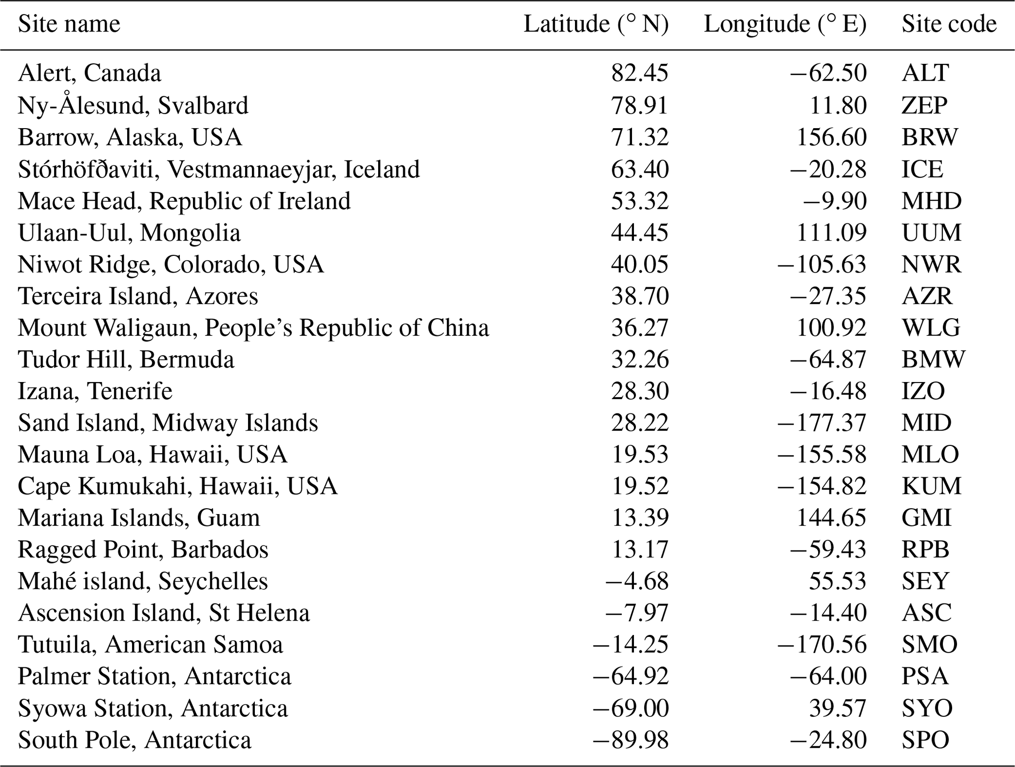
Table 1 List of 22 NOAA sites used in the analysis (Dlugokencky et al., 2021).

CH₄ has a mixture of natural and anthropogenic sources and chemical sinks, which lead to a strong seasonal cycle in the atmosphere. Figure 1 shows the mean seasonal cycle across NOAA observation sites (Table 1) in the Northern and Southern hemispheres, where concentrations are at a minimum in summer and peak in winter or early spring, depending on the location. The atmospheric CH₄ seasonal cycle is driven by the seasonal variations in the sources, such as wetlands, rice paddies and biomass burning, the chemical loss of CH₄ in the atmosphere, and the transport of CH₄. The main sources which drive the CH₄ cycle are dependent on climatological and meteorological conditions. Emissions from wetlands and rice paddies vary seasonally, with changes in temperature, precipitation, and soil moisture. Biomass burning emissions in the tropics and boreal regions also vary seasonally (Dlugokencky et al., 1997). It is thought that anthropogenic emissions play a smaller role in the seasonal cycle of CH₄ (e.g. Meirink et al., 2008; Wilson et al., 2021), but few studies have investigated the long-term influence of anthropogenic emissions on the observed seasonal cycle. For example, anthropogenic emissions might increase in winter due to increased gas extraction (Nisbet et al., 2019). The sinks of CH₄ also play a large role in the seasonal cycle. The main sink of CH₄ is the hydroxyl radical (OH), which is photochemically produced and results in the local abundance of OH varying seasonally due to the availability of UV radiation. Finally, transport of CH₄ in the atmosphere through advection, convection, and global circulation transporting air to the poles also influences the seasonal cycle.

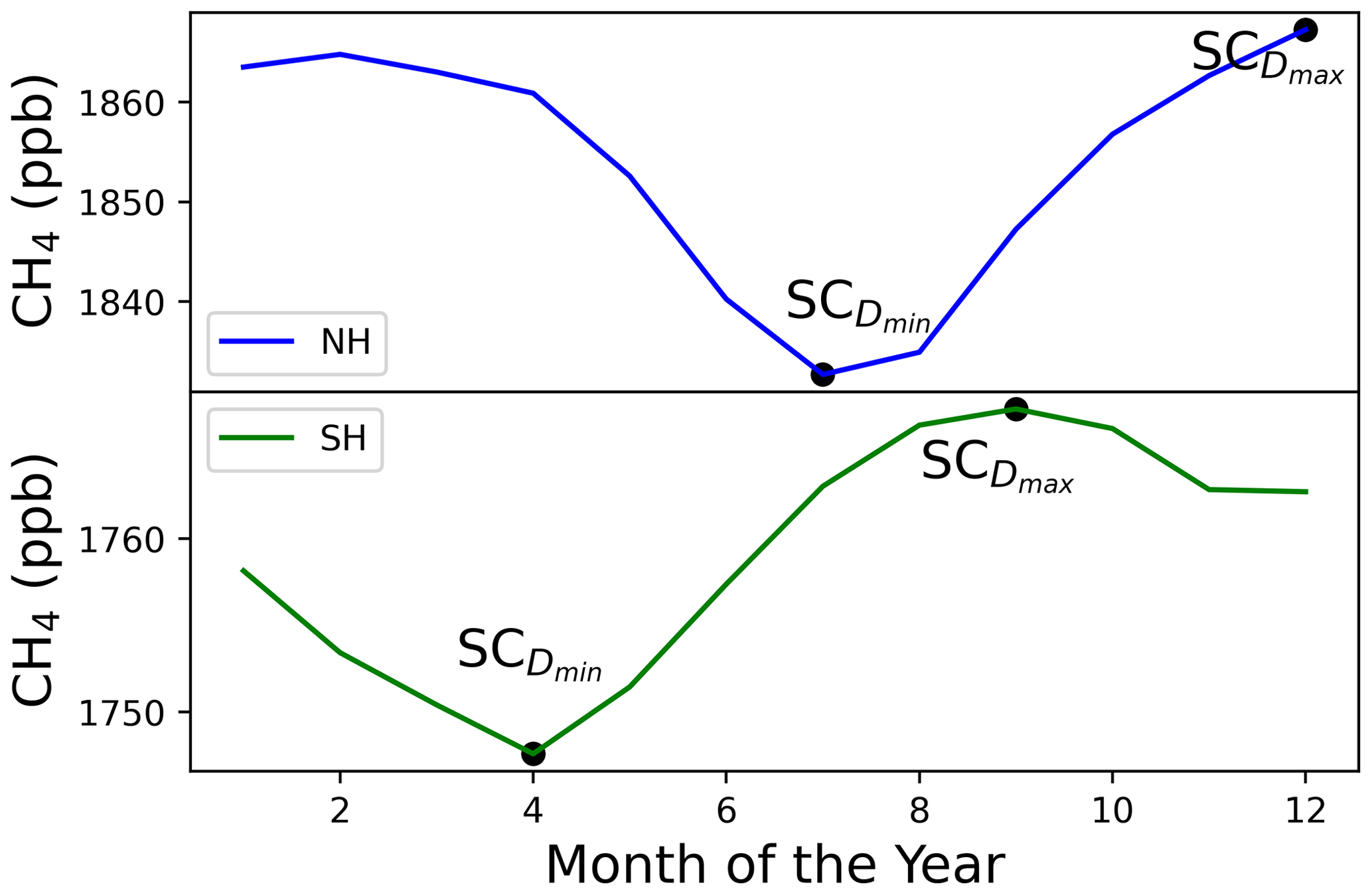
Figure 1 The monthly mean CH₄ mixing ratio (ppb) across the Northern Hemisphere (NH) and Southern Hemisphere (SH) at 22 NOAA surface sites between 1995–2022 (see Table 1). SC${}_{D_{max}}$ and SC${}_{D_{min}}$ represent the seasonal cycle maximum and minimum, respectively.

Many studies have assessed how well wetland models and chemical transport models reproduce the observed CH₄ seasonal cycle, the timing of the seasonal maximum and seasonal minimum, or what might be driving the seasonal cycle on a regional scale (Patra et al., 2011; Bergamaschi et al., 2018; Parker et al., 2020). These studies did not explore how the seasonal cycle amplitude (SCA) has changed over time on a global scale. The SCA is defined as the difference between the annual maximum and the annual minimum concentration at a particular location. Changes in the seasonality of emissions will be reflected in the seasonal cycle amplitude of CH₄ and will ultimately impact the annual growth rate. However, changes in loss rates and transport add extra complexity to the assessment of changes in the seasonal cycle. Studying the SCA could give us a better insight into changes in the CH₄ budget. In this study, we regionally attribute the change in SCA of CH₄ between 1995–2020, using the TOMCAT chemical transport model (Chipperfield, 2006) and surface observations from NOAA ESRL (Dlugokencky et al., 2021).

Note that, throughout this text, we are referring to concentrations when we use the term CH₄ alone. In Sect. 2, we describe the observations used, the modelling methodology, and the SCA analysis. In Sects. 3 and 4, we present our results and discuss our findings.

2 Methods

2.1 Atmospheric methane measurements

We assimilate and analyse the long-term surface flask measurements provided by NOAA ESRL. The air samples are collected approximately weekly or biweekly, and CH₄ is measured using gas chromatography with flame ionisation detection or by cavity ring-down spectroscopy methods (Dlugokencky et al., 2021). The NOAA observation network provides measurements across the globe, but there is a disproportionate number of sites in the Northern Hemisphere when compared with the Southern Hemisphere (see Fig. 2). There is also a lack of regular observations in some tropical regions, where there are large and uncertain CH₄ emissions.

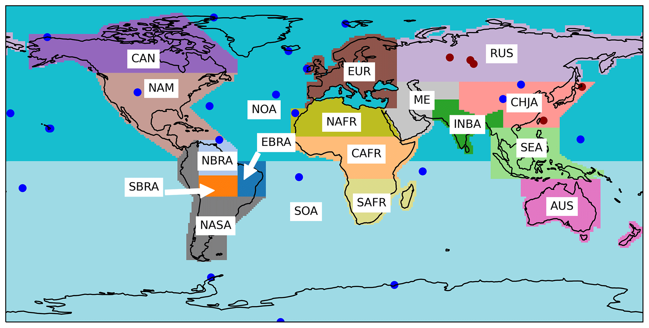
Figure 2 A map showing the 18 different regions selected for the tagged tracers, 22 NOAA surface observation site locations (blue), and the independent observations site locations (red). The observation sites shown in blue are the ones used to calculate SCA from 1995–2020.

We assimilate NOAA surface observations in INVICAT (Wilson et al., 2014), the inverse model of TOMCAT, in order to obtain optimised estimates of CH₄ fluxes to use in the TOMCAT forward model. We used observations from 80 NOAA surface observation sites and assimilated them at the correct model time step. Full details of the assimilation can be found in Sect. 2.3. In the SCA analysis, we used a subset of these observations. We calculated the monthly mean CH₄ at 22 NOAA surface sites, which were selected if they contained observations for the entire period of 1995–2020 and were not strongly influenced by local sources (McNorton et al., 2018). A list of the sites and their site codes are in Table 1, and their locations are shown by the blue dots in Fig. 2. We also evaluate the model performance using observations from the Center for Global Environmental Research, Earth System Division, National Institute for Environmental Studies, Japan (NIES; Tohjima et al., 2002; Sasakawa et al., 2010) and the Advanced Global Atmospheric Gases Experiment (AGAGE; Prinn et al., 2018a), which have not been assimilated (see Fig. S1 in the Supplement). The sites from NIES are in Siberia and East Asia, and the site from AGAGE is situated in the Republic of Ireland; their locations are shown as the red dots in Fig. 2. The independent observations do not cover the whole study period, but we have maximised the time period available from each data set by selecting a period with the most regular observations. The NIES observations in Siberia are from 2009–2015, the remaining NIES observations are from 1997–2015, and the AGAGE observations are from 1996–2020.

2.2 Tagged transport simulations

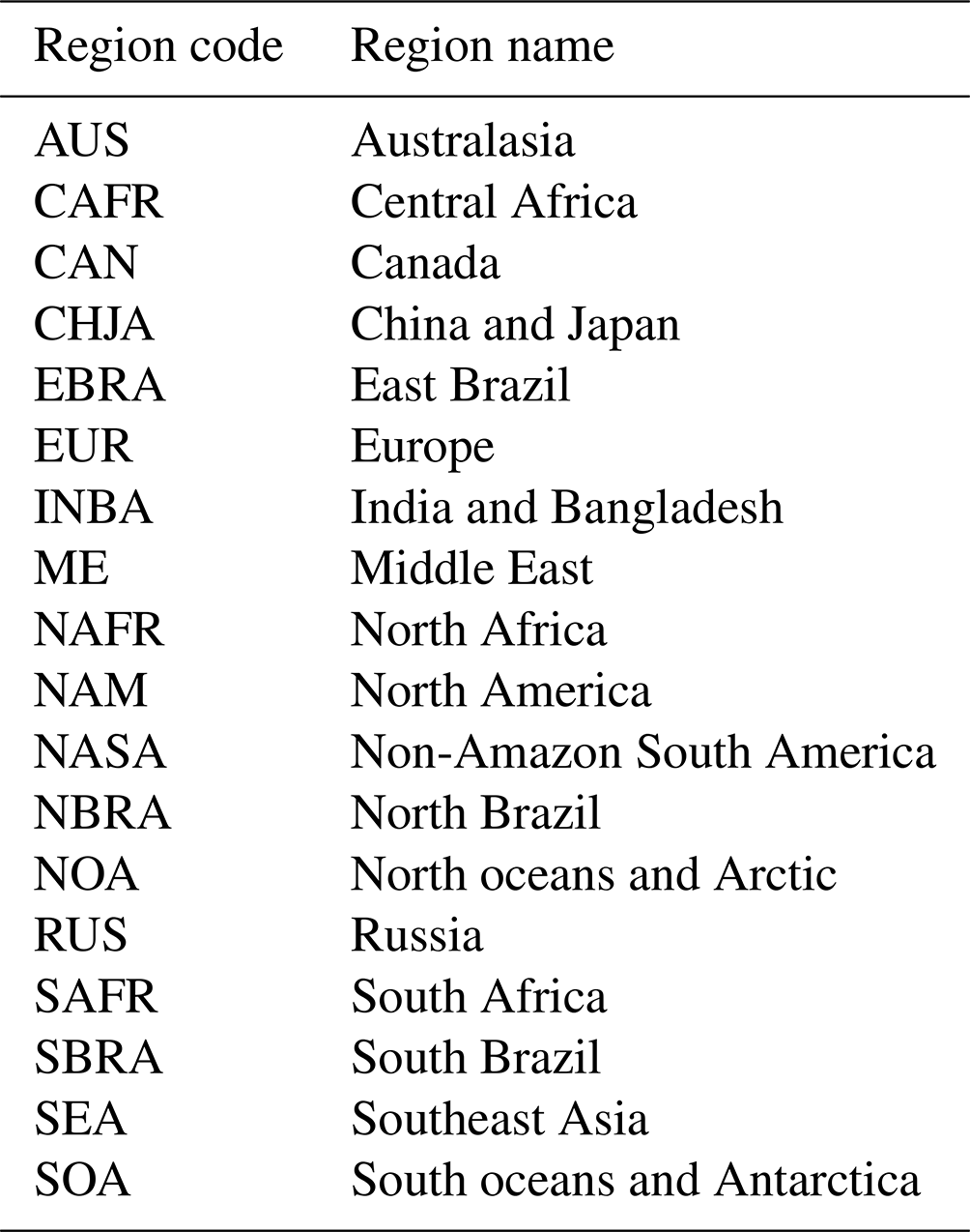
TOMCAT is a three-dimensional (3D) atmospheric chemical transport model which has been used in a number of studies to model CH₄ and other chemical species in the atmosphere (e.g. Chipperfield, 2006; Parker et al., 2018; Wilson et al., 2021). We use TOMCAT to investigate changes in the SCA of CH₄ between 1995 and 2020, including the impact of changes in emissions and transport. The globe was divided into 18 different regions, as shown in Fig. 2, in order to attribute the changes in the SCA from particular regions. The regions were selected based on the magnitude and type of emission in the distribution used in TOMCAT. The northern oceans, Greenland, Iceland, and Svalbard have been grouped together (north oceans and Arctic, NOA), as were the southern oceans and Antarctica (SOA). Northern land regions have been split into Canada (CAN), Europe (EUR), and Russia (RUS) due to their emission types and geographical location. The emissions from these regions include anthropogenic emissions, such as those from oil and gas industries, livestock, and other agriculture, and also include natural emissions, such as those from wetlands and biomass burning. In the northern mid-latitudes, regions such as North America (NAM), the Middle East (ME), and China and Japan (CHJA) are dominated by large anthropogenic emissions. Africa has been split into three regions because of the influence of central Africa in the CH₄ budget, with recent studies highlighting the large role that tropical wetlands play in the recent global growth of CH₄ (Lunt et al., 2021; Feng et al., 2022). Similarly, Brazil has been split into three regions due to the local emission sectors and different responses to seasonal changes in meteorology (Wilson et al., 2021; Basso et al., 2021). The north Brazil (NBRA) emissions are mostly driven by wetlands, whereas east Brazil (EBRA) is more susceptible to biomass burning in the arc of deforestation, a region of regular and intense anthropogenic burning. The south Brazil (SBRA) emissions are driven by a mixture of both wetlands and biomass burning. The rest of South America has been grouped as non-Amazon South America (NASA). Emissions from the Southeast Asia region (SEA) are from a mixture of rice paddies, biomass burning, and other anthropogenic emissions, whilst Australasia (AUS) is mostly driven by anthropogenic emissions, such as those from coal mines. The names given to each region are given in Table 2.

Table 2 List of 18 regions and their region code for each tracer.

Emissions from each region were simulated separately in the model and could be summed to represent global CH₄. This is possible due to the linearity of the TOMCAT model transport (Wilson et al., 2016) and offline (non-interactive) loss rates. In reality, the loss of CH₄ is not linear because the abundance of CH₄ impacts its rate of loss due to its impact on OH abundance, but this is a small effect relative to the large CH₄ abundance.

TOMCAT was run at a 5.6^∘ × 5.6^∘ horizontal resolution, with 60 vertical levels up to 0.1 hPa, between 1983 and 2020 for each regional tagged tracer, a background tracer, and a total CH₄ tracer. The background tracer contains CH₄ from the regional tracers once the CH₄ from each region has become well mixed. Each regional tagged tracer was set to be reallocated into the background tracer, using an exponential 9-month decay rate. Typical timescales for horizontal transport in the troposphere from the mid-latitudes to the poles is approximately 1–2 months, and interhemispheric transport is approximately 1 year (Jacob, 1999). The 9-month decay rate was selected in order to maximise the opportunity for CH₄ to undergo long-range transport from emission locations to surface sites, while minimising the effect of well-mixed atmospheric CH₄ on the results. The background tracer allows us to reduce the spin-up time required in the model to reach a steady state. Without the background allocation, concentrations would continue to increase because it takes approximately 20 years for the CH₄ to reach a steady state in the model. The background tracer also allows us to regionally attribute changes in the SCA, while accounting for well-mixed CH₄.

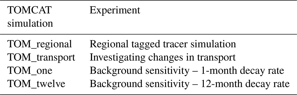
The study period begins in 1995 to allow the tracers to become well-mixed in the preceding 12 years. This model simulation is called TOM_regional and uses surface fluxes derived from a TOMCAT-based atmospheric inversion (described in Sect. 2.3). The meteorology was driven by the European Centre for Medium-Range Weather Forecasts (ECMWF) ERA5 reanalyses (Hersbach et al., 2020), and the OH fields for the troposphere and stratosphere were based on those within the TransCom-CH₄ study (Patra et al., 2011). The OH fields were originally taken from Spivakovsky et al. (2000) and scaled downwards by 8 %, in accordance with Huijnen et al. (2010), in order to match the observed methyl chloroform concentrations in the atmosphere (Patra et al., 2011). The stratospheric loss rates for Cl and O(¹D) varied annually and were taken from a previous full chemistry TOMCAT simulation (Monks et al., 2017). The soil sink was taken from the Soil Methanotrophy Model (MeMo) model, which varied each year between 1990 and 2009; the 1990 values were annually repeated from 1983–1990, and similarly, the 2009 values were repeated annually from 2009–2020 (Murguia-Flores et al., 2018).

We carried out two sensitivity experiments to investigate the impact of the choice of the exponential lifetime used to allocate well-mixed CH₄ into the background tracer and to investigate if it influences the background tracer's contribution to the change in the SCA. Decay rates of 1 and 12 months were selected to show the impact of a short and long decay timescales on the background and regional contributions of the change in the SCA. The simulations are labelled TOM_one for the 1-month decay rate and TOM_twelve for the 12-month rate. The results of the sensitivity experiments can be found in Sect. 3.5.

The TOM_regional simulation quantifies the impact that the regional emissions have on the SCA of CH₄ elsewhere under annually varying transport processes. In order to investigate the role that those transport processes alone play in the change to the SCA of CH₄, we also carried out a separate regional tagged tracer simulation using annually repeating emissions for the same time period. Using annually repeating values removes the influence of changing emissions, allowing us to investigate changes to the transport undergone by emissions from each region over time. The surface emissions for each month of the year were averaged between 1983–2020. These emissions were repeated annually, using the same model set-up as TOM_regional, and the same analysis of SCA was repeated for 1995–2020. This constant emissions simulation is labelled TOM_transport. A summary of the TOMCAT simulations can be found in Table 3.

Table 3 List of the different TOMCAT simulations.

2.3 Fluxes from atmospheric inversions

The surface fluxes for the tagged tracer simulations were derived using the TOMCAT-based inverse model, INVICAT (Wilson et al., 2014). INVICAT has been used in a number of studies to constrain the emissions of various species, including CH₄ (Gloor et al., 2018; Wilson et al., 2021). It uses a 4D-Var variational method, based on the one used in numerical weather prediction, with full details on the methods used in INVICAT given in Wilson et al. (2014). The inverse method aims to minimise the value of a cost function in a least squares sense. The cost function combines an error-weighted sum of the differences between the model and observations and the uncertainty-weighted sum of changes to the a priori flux estimate (Wilson et al., 2021). The input for INVICAT includes an a priori mean flux value for each grid cell and an error covariance matrix containing the covariances between the flux uncertainties. The output is an a posteriori mean grid cell flux and error covariance matrix. The a priori and a posteriori fluxes will hence be referred to as prior fluxes and posterior fluxes, respectively.

The inverse model simulations were run at a 5.6^∘ × 5.6^∘ horizontal resolution, with 60 vertical levels up to 0.1 hPa and a time step of 30 min. The meteorology was taken from ECMWF's ERA5 reanalyses (Hersbach et al., 2020). An inversion was carried out separately for each year and completed 40 minimisation iterations. The 40 iterations were sufficient for the cost function and its gradient norm to be judged as converged, based on both being smaller than 1 % of their initial value. The inversion for each year was run for 14 months, until February the following year, in order to better constrain the fluxes in the final months of each year. The final 2 months of each year are discarded from the results. Each inversion overlapped with the following one by 2 months to give the transport of fluxes time to reach measurement sites. The overlapping months were initialised using 3D fields provided from the correct date in the previous year, so the total CH₄ burden was conserved across each year.

The 4D-Var-simulated CH₄ mixing ratios were linearly interpolated to the correct longitude, latitude, and altitude of each surface observation used in the inversion at the nearest model time step. The surface observations were given uncorrelated errors of 3 ppb (parts per billion) plus a representation error. The representation error was estimated as being the mean difference across eight grid cells around the cell which contained the observation. The prior emissions were taken from various inventories. The anthropogenic emissions were taken from EDGARv5 (Crippa et al., 2021), excluding rice paddies and fires. The biomass burning emissions were taken from GFEDv4.1s (Randerson et al., 2017). The WetCHARTs model (Bloom et al., 2017) in a median set-up was used for the wetland fluxes. The median set-up uses the median scaling factor and temperature response from the WetCHARTs suite and the Global Lakes and Wetlands Database distribution of wetlands. The wetland fluxes were then masked to remove emissions which overlap with rice emissions and then scaled back up to 180 Tg to match the top-down mean value from the global methane budget (Saunois et al., 2020). The rice and termite emissions were taken from the TransCom intercomparison project (Patra et al., 2011). The termite emissions were scaled to match the total quoted in Saunois et al. (2020). The geological emissions were from Etiope et al. (2019), and the ocean emissions are taken from Weber et al. (2019). The prior emissions are given cell uncertainties of 250 % of the prior flux value and also include 500 km spatial correlations, with a Gaussian distribution for all fluxes. Fossil fuel fluxes have temporal correlations, based on an exponential distribution with a timescale of 9 months. The tropospheric and stratospheric loss rates are the same as those used in the TOMCAT tagged tracer simulations (Sect. 2.2).

2.4 Data processing and analysis

The monthly mean model output from TOMCAT was interpolated horizontally and vertically to the 22 surface observation sites (Table 1) from NOAA's ESRL (Dlugokencky et al., 2021) to check the model performance and in order to investigate the regional contribution to the change in SCA at these sites. Following methods used by Lin et al. (2020) for CO₂, the seasonal cycle amplitude (SCA) of CH₄ and the regional contribution to the SCA was analysed.

To calculate the SCA, we isolate the mean annual cycle observed in CH₄ by taking the interpolated model output at each surface observation site and then smoothing and detrending the time series using the CCGCRV curve-fitting routine, as developed by Thoning et al. (1989). CCGCRV approximates the seasonal cycle and long-term trend variation by fitting a polynomial equation combined with a harmonic function (Pickers and Manning, 2015). The short-term and long-term cutoff values can be selected, and we chose 80 and 667 d cutoffs, respectively (Dlugokencky et al., 1994). These parameters have been used in previous studies (Dlugokencky et al., 1994; Parker et al., 2018). The SCA for the observations and the modelled total tracer were calculated by taking the difference between the annual maximum $\left({\mathrm{SC}}_{D_{max}}\right)$ and annual minimum $\left({\mathrm{SC}}_{D_{min}}\right)$ of the detrended curve:

$$\begin{array}{}\text{(1)}& \mathrm{SCA}={\mathrm{SC}}_{D_{max}}-{\mathrm{SC}}_{D_{min}},\end{array}$$

where D_max and D_min are the days of the annual CH₄ cycle maximum and minimum. For each tagged regional tracer, i, a pseudo SCA (SCA^′) was calculated, where the pseudo maximum $\left({\mathrm{SC}}_{i,D_{max}}^{\prime }\right)$ or minimum $\left({\mathrm{SC}}_{i,D_{min}}^{\prime }\right)$ is the point of its annual cycle corresponding to D_max and D_min. The pseudo seasonal cycle amplitude was calculated as follows:

$$\begin{array}{}\text{(2)}& {\mathrm{SCA}}_i^{\prime }={\mathrm{SC}}_{i,D_{max}}^{\prime }-{\mathrm{SC}}_{i,D_{min}}^{\prime }.\end{array}$$

The pseudo SCA was defined to account for the difference in the timing of the local D_max and D_min of the individual tracers and observed CH₄ at the observation sites. The total change in SCA over the study period, ΔSCA (ppb), was derived by calculating the linear trend (k_SCA) in the SCA and multiplying it by the number of years in the study (n_year; 25 years):

$$\begin{array}{}\text{(3)}& \mathrm{\Delta }\mathrm{SCA}=k_{\mathrm{SCA}}\times n_{\mathrm{year}}.\end{array}$$

Once the SCA and ΔSCA were calculated, the surface sites were then grouped into five latitude bands for further analysis. These groups are northern high latitudes (NHLs; 60–90^∘ N), northern mid-latitudes (NMLs; 30–60^∘ N), northern tropics (NTrs; 0–30^∘ N), southern tropics (STrs; 0–30^∘ S), and southern high latitudes (SHLs; 60–90^∘ S). There are no surface observations from the southern mid-latitudes (SMLs; 30–60^∘ S), so we do not analyse the SCA in this latitude band.

The main sink of CH₄ is through a reaction with OH, and the rate of removal is dependent on temperature and the amount of CH₄ and OH in the atmosphere (Dlugokencky et al., 1997). The atmospheric burden of CH₄ has been increasing, and it is expected that the SCA of CH₄ would increase due to more CH₄ being removed by OH in the atmosphere, assuming that OH concentrations remain relatively constant during this time. To account for the impact of OH on ΔSCA, we calculated the amount of CH₄ lost by OH across the whole atmosphere in each month of the study period:

$$\begin{array}{}\text{(4)}& {\displaystyle }{L}_{{\mathrm{CH}}_{\mathrm{4}}}=m_{{\mathrm{CH}}_{\mathrm{4}}}\left(\mathrm{1}-e^{-k\left[\mathrm{OH}\right]\mathrm{\Delta }t}\right)\text{(5)}& {\displaystyle }k=\mathrm{2.45}\times {\mathrm{10}}^{-\mathrm{12}}{e}^{(-\mathrm{1775}/T)},\end{array}$$

where $L_{{\mathrm{CH}}_{\mathrm{4}}}$ is the amount of CH₄ lost (kg) in each model grid box through the reaction with OH in 1 month, and $m_{{\mathrm{CH}}_{\mathrm{4}}}$ is the mass of CH₄ (in kg) in each grid box. The variable k is the reaction rate constant (in cm³ molec.⁻¹ s⁻¹; Eq. 5; where T is temperature in Kelvin), [OH] is the amount of OH (molec. cm⁻³), and Δt is number of seconds in 1 month. $L_{{\mathrm{CH}}_{\mathrm{4}}}$ was converted (to ppb), and a mean monthly loss was calculated for the Northern and Southern hemispheres across all the vertical model levels over the study period. The loss was then smoothed and detrended, using the CCGCRV curve-fitting routine, and ΔSCA was calculated using the same method described above. It is not realistic to account for the contribution to ΔSCA from loss by OH at individual surface sites because this would not capture the seasonal cycle of OH in the mid-troposphere, where the majority of CH₄ loss by OH occurs. This makes it difficult to relate the seasonal changes in CH₄ due to losses of OH at particular sites, which is why we have calculated $L_{{\mathrm{CH}}_{\mathrm{4}}}$ as a mean across the Northern and Southern hemispheres.

3 Results

3.1 Observed ΔSCA

The observed ΔSCA was calculated at the 22 observations sites. We find that the global mean SCA at available sites is increasing, but there are different regional trends, for example, in the NHLs, the observed ΔSCA decreased at all sites between 1995–2020 (Fig. 3). The observed global mean value of ΔSCA was 2.5 ppb, corresponding to an increase in the SCA by 6.5 %. The reaction between CH₄ and OH is dependent on the amount of CH₄ available in the atmosphere. The combination of the increasing CH₄ burden in the atmosphere and the photochemically driven seasonal variation in the OH results in more CH₄ being removed from the atmosphere during the time of maximum OH. Therefore, an increase in the global mean SCA is expected due to the increasing atmospheric burden of CH₄. However, when we look at the ΔSCA latitudinally, there are large differences in the NHLs compared to the rest of the world. The mean observed ΔSCA in the NHLs was −4.0 ppb, which represents a 7.6 % decrease between 1995 and 2020, and in the non-NHL region, the mean observed value of ΔSCA was 4 ppb, which is an increase of 11.5 % for the study period. The reasons for this widespread contrasting behaviour in the NHLs compared to the rest of the world is investigated in more detail in the forthcoming sections.

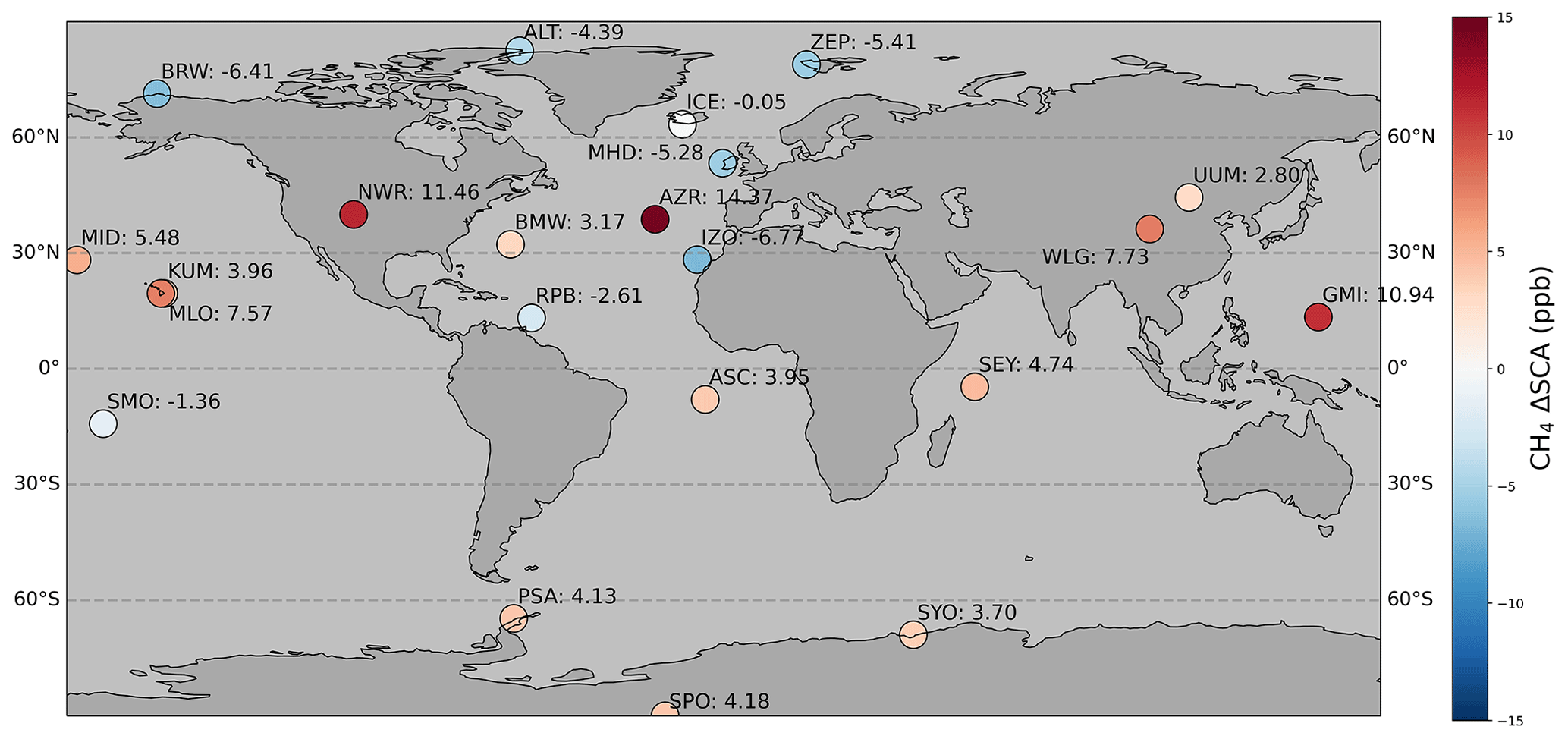
Figure 3 Map showing ΔSCA (ppb) at the 22 selected observation sites.

The distribution of ΔSCA at sites in non-NHL regions is quite variable. For example at NWR, AZR, and GMI, ΔSCA is large and positive, but other sites such as MHD, IZO, and SMO have negative ΔSCA values. The sites with the largest positive ΔSCA (e.g. NWR, BRW, AZR, GMI, and WLG) are most likely influenced by outflow from the USA and Asia. The sites with large positive ΔSCA and negative ΔSCA in the non-NHL regions do not have a strong regional or local pattern in ΔSCA, unlike in the NHLs. All four sites in the NHLs display contrasting behaviour and have a negative ΔSCA compared to the rest of the world; therefore, the NHLs will be the main focus of our analysis.

BRW, ALT, and ZEP have a ΔSCA which ranges from −4 to −5 ppb. The SCA at these sites is variable but has a strong decreasing trend. ICE has a smaller ΔSCA (−0.05) ppb compared the other three sites in the NHLs. There is a large decrease in the SCA during the first 4 years of the study, and then the SCA value steadily fluctuates between ∼ 30 and ∼ 40 ppb. This results in no trend in the SCA for the rest of the study period, resulting in a smaller negative ΔSCA compared to the other sites (see Fig. S2 in the Supplement).

The non-NHL regions had a mean observed ΔSCA of 4 ppb. The three SHL sites sample well-mixed air and are less influenced by local sources. The concentrations at regional sites near to emissions are all affected in different ways, whereas at the sites in Antarctica, the effect is smoothed out by the time air reaches the South Pole region. The three sites in Antarctica are exposed to well-mixed air and have the same mean increase of 4 ppb, highlighting that the observed ΔSCA in NHLs is very different to the global observed ΔSCA. This implies that the Arctic is responding differently to the global increase in CH₄ concentrations compared to the rest of the world, and therefore, we focus on investigating the decreasing SCA in the NHLs.

3.2 Model evaluation

The observed CH₄ SCA is simulated well by TOMCAT with the surface fluxes from INVICAT in the TOM_regional simulation (Fig. 4a). There is a strong linear relationship between the modelled and observed SCA, with a mean bias of 0.93 ± 0.09 ppb. However, the model struggles to capture the SCA at Mount Waligaun (WLG) in China. This is likely due to the fact that it has the highest altitude out of all the sites, and the reasonably coarse model grid cell will not capture the local topography. The model simulation was also compared with sites that were not assimilated in INVICAT, although there are limited observations, with only six sites situated in the northern tropics and northern mid-latitudes. Due to these sites only having regular observations over a short time period, the comparison only covers the periods 1997–2015 and 2009–2015 (see the Supplement). The model captures the SCA well at these independent sites, apart from Cape Ochi-ishi (COI), where the model has a weaker seasonal cycle, particularly during the seasonal cycle minimum. COI is situated near swamps, grazing lands, and two cities, so it is possible that the model does not fully capture the complexity of the local sources well. There are large error bars (1σ) for the Siberian sites in both the modelled and observed SCA. This is due to the SCA being quite variable over the short time period available. However, the model still compares well with the observed SCA at these sites, with a mean overestimation of 16 ppb, which is well within the 1σ error. Full results of the independent analysis can be found in the Supplement (Fig. S1). The model captures the mean SCA well, when compared with NOAA observation sites, but there are larger differences with the independent sites, which is due, in part, to larger variability in the SCA over a shorter time period.

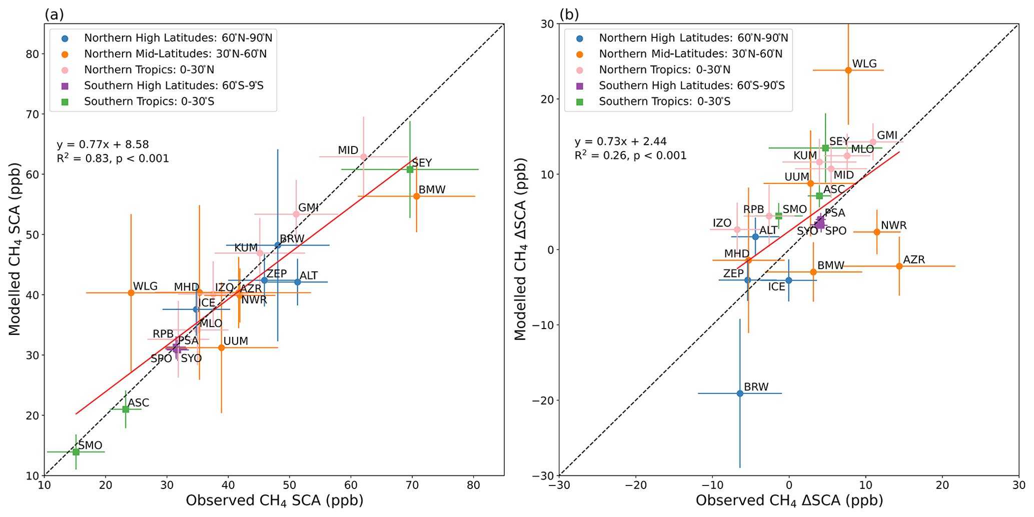
Figure 4 Comparison between simulated and observed (a) CH₄ SCA (ppb) and (b) CH₄ ΔSCA (ppb). The SCA shown is the mean SCA between 1995–2020, and ΔSCA is the change in SCA for the same period. The dashed black line represents the 1 : 1 line, and the red line represents the least squares regression line. The error bars denote ±1σ, which represents the interannual variability between 1995–2020.

The model also captures ΔSCA well when compared with observations, including the negative ΔSCA and contrasting behaviour in the NHLs shown by observations (Fig. 4b). As a result, we can use TOMCAT to inform us on what might be driving this significantly different behaviour in the NHLs. There is a good correlation (r=0.51) between the model and observations, and they almost always match within the 1σ uncertainty in the observations, with some outliers. At ALT, TOMCAT shows a ΔSCA of 1.7 ppb, and this is due to TOMCAT underestimating the SCA when compared with observations, particularly at the beginning of the study period. At BRW, the model has a much stronger negative ΔSCA when compared with the observations, and this is due to the model overestimating the SCA at the beginning of the study period. Despite the under- and overestimations at these two sites (ALT and BRW) in the NHLs, the mean value of ΔSCA in TOMCAT is −6.38 ppb in the NHLs, which shows a larger negative trend in the SCA than the observed mean ΔSCA value of −4 ppb. This is mostly due to the overestimation of the magnitude of the simulated ΔSCA at BRW. At WLG, the model overestimates ΔSCA; again, this is likely due to the model representation at this site. The time series of the SCA and its trend at each NOAA site can be found in the Supplement. The model performs better at the NOAA sites, partly because these sites are used to provide optimised fluxes in our model and because ΔSCA was calculated over a long time period of 25 years. The independent site at Mace Head (GC-MD) also performs well because ΔSCA is calculated over a period of 18 years. The independent sites in Siberia do not perform as well, compared to GC-MD and the NOAA sites, because of the large variability in the SCA over the relatively short time period (6 years) of observations. Despite some differences between the model and observations in the NHL and non-NHL regions, the model still captures the change in the SCA across the globe, almost all within 1σ uncertainty in the observations. We are confident that the transport in the model is sufficient. Therefore, we can use TOMCAT to regionally attribute the changes in the SCA in the NHL.

3.3 The role of OH

We use the TOM_regional simulation to determine the influence that the increasing abundance of CH₄ in the atmosphere has on its removal by OH and the seasonal cycle. In the TOM_regional simulation, we use OH fields which vary from month to month but do not vary from year to year due to uncertainty in the annual variability. Some studies find a declining trend in OH from 2004 (Rigby et al., 2017; Turner et al., 2017), but Zhao et al. (2019) found an increasing trend in OH between 2000 and 2010. In contrast, some studies only find small annual variability in OH (Patra et al., 2021; Naus et al., 2021). These studies contain large uncertainties and do not cover the full period of our study, so a year-to-year variability in OH was not included our TOMCAT simulations.

Using TOMCAT, we find that, in the Northern Hemisphere, the ΔSCA due to OH loss is +1.0 ppb, and it is +1.1 ppb in the Southern Hemisphere. Based on these findings, we would expect the observation sites to show a ΔSCA of ∼ 1 ppb in the absence of any other changes and that any deviations from that are due to changes in transport and/or emissions. These results inform our expectation that the SCA is expected to increase with the increasing atmospheric burden of CH₄, due to more CH₄ being removed by OH.

3.4 Regional contribution to ΔSCA in northern high latitudes

We now assess what is driving the decreasing SCA in the NHLs by analysing the regional contributions at NHL sites in the TOM_regional simulation. Figure 5 shows the contribution of the background and tagged regions as a mean across all sites in each latitude band. The background tracer shows the largest contribution to negative ΔSCA in the NHLs (−9.93 ppb; Fig. 5a). The background tracer represents the CH₄ that is well-mixed in the atmosphere, likely from emissions from distant regions. The largest regional contributors to the negative ΔSCA in the NHLs include Canada (−2.97 ppb), the Middle East (−2.13 ppb), and Europe (−1.48 ppb), as shown in Fig. 5b. The China and Japan region has the largest positive influence on NHL ΔSCA (3.94 ppb). Despite some positive regional contributions of ΔSCA to the NHLs, the ΔSCA in the NHLs is still decreasing. This is due to the negative contribution of well-mixed emissions from the background tracer and large regional negative contributions from Canada, Europe, and the Middle East.

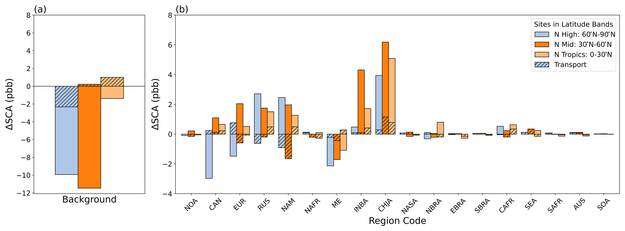
Figure 5 The contribution of the (a) background tracer and (b) regional tagged tracers to CH₄ ΔSCA (ppb) for 1995–2020 as a mean across all sites in the latitude band. The blue bars show the NHLs, and the orange bars are the two non-NHL bands in the Northern Hemisphere. The hatched bars show the contribution from transport (TOM_transport), and the solid colour represents the contribution from emissions (TOM_regional). Note that panels (a) and (b) have different scales.

The TOM_transport simulation represents the contribution of transport to the negative ΔSCA in the NHLs, and this simulation shows a different regional contribution compared to the TOM_regional simulation (Fig. 5; TOM_transport simulation is represented by the hatched bars). From this simulation, we find that 33 % of the negative ΔSCA in the NHLs is due to changes to transport, and this can be split into contributions from the background and regional tracers. The largest contribution from transport as a fraction of the total contribution of the tracer is from the background tracer, which accounts for 23 % (−2.32 ppb). Changes in the transport of emissions from North America and Russia have also contributed to the decrease in the SCA between 1995–2020 in the NHLs; however, the changes in emissions from these regions contribute to an increase in the SCA. The change in SCA due to emissions is larger in magnitude than the contribution from transport, resulting in overall increase in the SCA in the NHLs from these regions. The TOM_transport contribution to ΔSCA in NHLs from Canada and Europe is 0.24 and 0.77 ppb, respectively, resulting in an increase in the SCA in the NHLs due to changes in transport. However, changes in emissions result in an overall decrease in the SCA from these regions. This is due to the magnitude of the decrease in SCA being larger than the contribution from transport. This implies that their contributions to the negative ΔSCA in NHLs are due to changes in emissions. We also assess the effect that the size of the regional tracers has on our results by normalising the regional contribution by area size. We find that the largest contributors to the decreasing SCA in the NHLs are still due to changes in emissions from Canada, the Middle East, and Europe (see Fig. S3 in the Supplement).

The TOMCAT simulations (TOM_regional and TOM_transport) show that the largest contributions to the decrease in ΔSCA in the NHLs are mostly due to changes in emissions from Canada, the Middle East, and Europe. To further investigate the changes in emissions that are driving the negative ΔSCA in the NHLs, we look at the trends of the regional CH₄ concentration (ppb) contributions from the TOM_regional and TOM_transport simulation as a mean across all sites in the NHLs. We refer to these regional CH₄ concentration contributions as being the tracer contribution. We also assess the trends of the seasonal emissions from each region. Often the trends in both the CH₄ contributions and the regional emissions are not statistically significant due to their large variability over time. However, we are interested in the direction of these trends in order to determine how emissions and transport from each region are changing over time and their impact on the seasonal cycle in the NHLs. We compare the seasonal trends of regional tracer contributions (ppb) to the NHLs from the TOMCAT_regional and TOMCAT_transport to further assess the contribution of emissions and transport from individual tracers. If the trend in the TOMCAT_transport simulation is comparable to the trend in the TOMCAT_regional simulation, then we can attribute the change to transport and not emissions. To assess the change in the seasonal emissions, we calculated the interseasonal range (ISR; Tg per month), which represents the difference between the June, July, and August (JJA) and December, January, and February (DJF) seasonal mean emissions. It is important to note that the emission seasonal cycle is out of phase with the concentration seasonal cycle at northern mid- and high latitudes, so a positive ISR in the emissions leads to a decreasing SCA. This is because the CH₄ seasonal cycle minimum is during the summertime in the NHLs, so increasing emissions during this time would raise the minimum value, thereby shrinking the seasonal cycle. Similarly, shrinking wintertime emissions would bring down the seasonal maximum which occurs at the same time. This effect is mostly likely in regions near to sites in the NHLs. We focus on the three largest regional contributors to the negative ΔSCA in the NHLs, namely Canada, Europe, and the Middle East. We also focus on the largest regional positive contributor of ΔSCA in the NHLs, China and Japan, to assess its impact on the decreasing SCA at NHL sites.

When we look at the regional tracer contributions in the NHLs from Canada and Europe, we find stronger trends in the TOM_regional simulation, compared to no trends shown in the TOM_transport simulation during DJF and JJA seasons (Figs. 6a and 7a). This shows that changes in emissions in these regions are driving the decrease in the NHLs. This is also shown by a positive ISR in emissions from Canada and Europe (Figs. 6b and 7b). The Middle East's tracer contribution in the NHLs shows no trends in the TOM_transport simulation, which means that the changes in transport from this region have very little impact on the SCA in the NHLs (Fig. 8a). As a result, changes in emissions in the Middle East are the mostly driving the decrease in the SCA in the NHLs. This is also shown by a positive ISR in the emissions from the Middle East (Fig. 8b). Changes in emissions are the main contributor to the decrease in the SCA in the NHLs from Canada, the Middle East, and Europe. China and Japan contribute the most to increasing the SCA in the NHLs; however, the overall changes in emissions and transport from the background tracer and other regions still result in a decreasing SCA. We find that a combination of changes in emissions and changes in transport from China and Japan are causing an increase in the SCA in the NHLs from this region (Fig. 9). By comparing the TOM_regional and TOM_transport simulations and the seasonal changes in emissions in these regions, we find that changes in emissions are the largest driver in changes in the SCA in the NHLs.

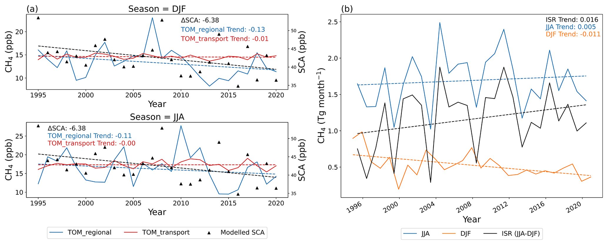
Figure 6 (a) Canada's seasonal mean CH₄ (ppb) contribution to the NHL sites (60–90^∘ N) for TOM_regional (blue) and the TOMCAT_transport simulation (red) for 1995–2020. (b) Canada's seasonal mean emissions (Tg per month) from the inversion for JJA (blue), DJF (orange), and the interseasonal range (ISR; black) for 1995–2020.

Changes in emissions from Canada are mostly driven by increasing JJA emissions and decreasing DJF emissions. The changes in seasonal emissions lead to a positive ISR (0.02 Tg per month per year; p value = 0.17; Fig. 6b). The trend of the DJF tracer contribution in the TOM_regional is decreasing at a faster rate (−0.13 ppb per month; p value = 0.13) than the JJA (−0.11 ppb per month; p value = 0.36), which results in a decrease in the SCA. There is some uncertainty in the trends of both the emissions and tracer contributions due to their large variability during the study period. The combination of weak trends in TOM_transport simulation and the positive ISR indicates that changes in DJF and JJA emissions from Canada are the main contributor to the decreasing SCA in this region.

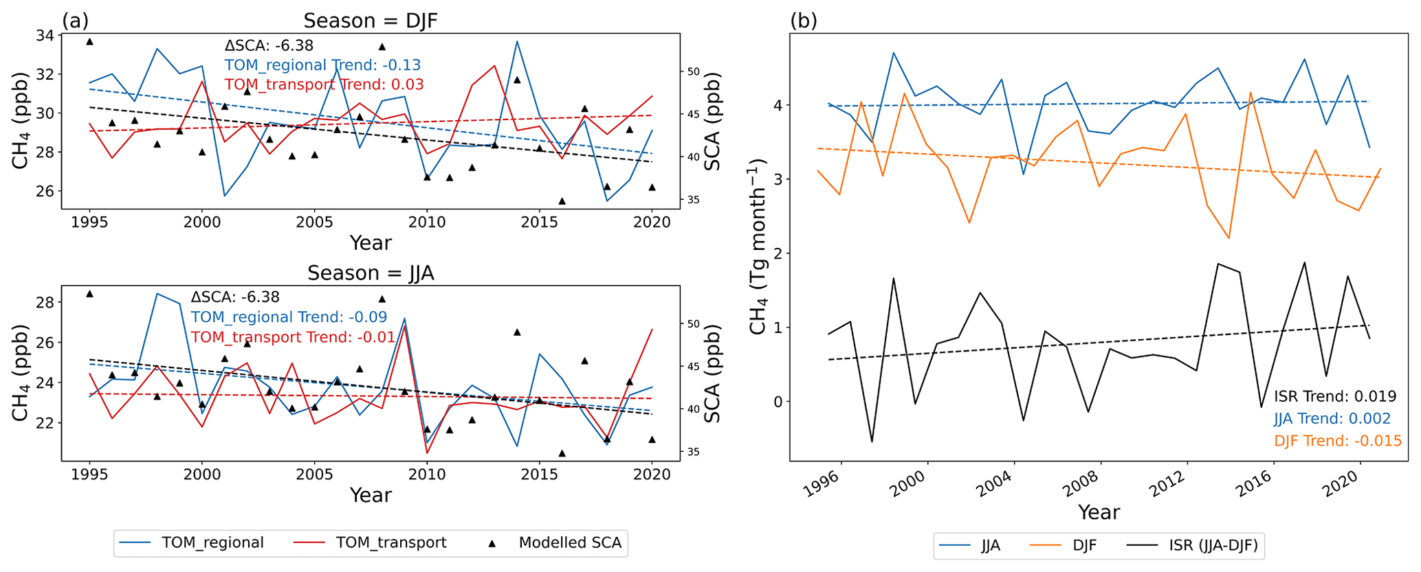
Figure 7 (a) Europe's mean CH₄ (ppb) contribution to the NHL sites (60–90^∘ N) for the TOMCAT_regional (blue) and the TOMCAT_transport simulation (red) for 1995–2020. (b) Europe's mean emissions (Tg per month) from the inversion for JJA (blue), DJF (orange), and the interseasonal range (ISR; black) for 1995–2020.

The emissions from Europe during JJA are increasing slightly, but there is a stronger decrease in the DJF emissions. The decrease in winter emissions result in a positive ISR (0.02 Tg per month per year; p value = 0.3; Fig. 7b). The mean CH₄ tracer contribution from Europe to the NHL sites in the TOM_transport simulation shows a small positive trend in DJF and a very small decreasing trend in JJA (Fig. 7a). This shows that changes in winter transport are contributing to an increase in the SCA in the NHLs. However, large variability in the TOM_transport concentrations leads to some uncertainty regarding how much transport is having an impact from this region. The changes in emissions in the TOM_regional simulation contribute more to a decrease in the SCA. The TOM_regional DJF tracer contributions (−0.13 ppb per month; p value = 0.02) from Europe are decreasing at a faster rate than the JJA tracer contributions (−0.09 ppb per month; p value = 0.06), resulting in a decrease in the SCA. The positive ISR is supported by trends in the tracer contributions being statistically significant, which shows that changes in emissions from this region are driving the decrease in NHLs.

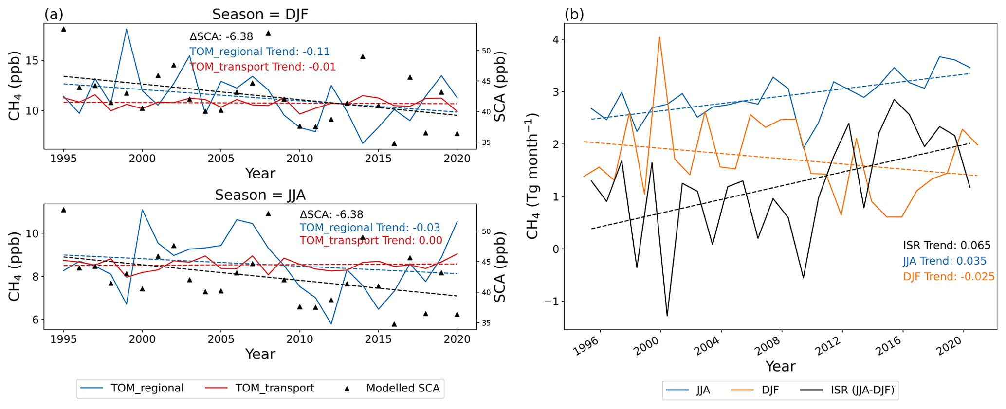
Figure 8 (a) The Middle East's mean CH₄ (ppb) contribution to the NHL sites (60–90^∘ N) for the TOM_regional simulation (blue) and the TOM_transport simulation (red) for 1995–2020. (b) The Middle East's mean emissions (Tg per month) from the inversion for JJA (blue), DJF (orange), and the interseasonal range (ISR; black) for 1995–2020.

The emissions from the Middle East are increasing in JJA and decreasing in DJF, which results in a positive ISR (0.07 Tg per month per year; p value = 0.01; Fig. 8b). The mean CH₄ tracer contribution from the Middle East to the NHL sites is decreasing in both JJA (−0.04 ppb per month; p value = 0.3) and DJF (−0.11 ppb per month; p value = 0.07) in the TOM_regional simulation (Fig. 8a). The trend in DJF is decreasing faster than the trend in JJA, resulting in a decrease in the SCA. The combination of the positive trend in the ISR being statistically significant and the rapidly decreasing winter concentrations indicates that changes in emissions from this region are the main contributor to the decrease in the SCA in the NHLs.

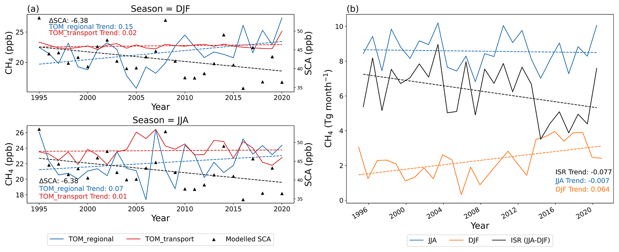
Figure 9 Panel (a) shows China and Japan's mean CH₄ (ppb) contribution to the NHL sites (60–90^∘ N) for the TOMCAT_regional (blue) and the TOMCAT_transport simulation (red) for 1995–2020. Panel (b) shows China and Japan's mean emissions (Tg per month) from the inversion for JJA (blue), DJF (orange), and the interseasonal range (ISR; black) for 1995–2020.

The emissions from China and Japan are decreasing slightly in JJA and increasing in DJF, resulting in a negative ISR (−0.07 Tg per month per year; p value = 0.05; Fig. 9b). The mean CH₄ tracer contribution from this region to the NHLs is increasing in DJF and JJA in the TOM_regional simulation (Fig. 9a). The DJF contribution is increasing at a faster rate (0.15 ppb per month; p value = 0.03) than the JJA contribution (0.07 ppb per month; p value = 0.21), resulting in an increase in the SCA. The TOM_transport simulation shows a small trend in DJF (0.015 ppb per month; p value = 0.32) in the tracer contribution from this region and no trend in the JJA contribution, showing that transport is also contributing to an increase in the SCA in NHLs. However, there is some uncertainty in terms of how much transport is having an impact, due to the large variability in the trends in the tracer contribution in the TOM_transport simulation. The TOMCAT simulations and emission trends show that changes in emissions and DJF transport from China and Japan contribute to an increase in the SCA in the NHLs. However, the overall contribution from the background tracer and other regional tracers still results in a decrease in the SCA in the NHLs.

3.5 Sensitivity experiments

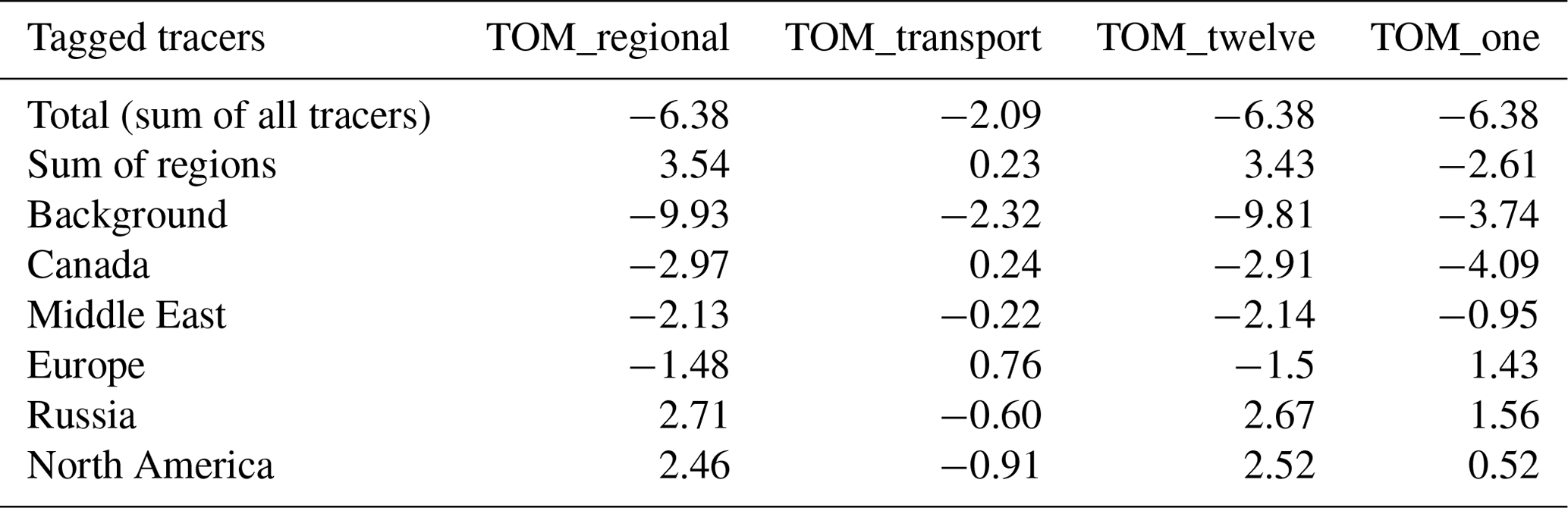
We carried out two sensitivity experiments to examine the impact of shorter and longer decay rates of regional tracers into the background tracer. These simulations are described in Sect. 2.2. The TOM_twelve simulation showed that changing the exponential decay rate from 9 to 12 months did not change the largest contributors to the ΔSCA. This implies that, after 9 months, CH₄ emissions have undergone long-range transport and no longer have a distinguishable emission origin and have become well mixed. Reducing the exponential decay rate to 1 month did, however, have an impact on the final results. The TOM_one simulation showed larger regional contributions in the NHLs from Canada than the background tracer. The contribution from the background tracer in the TOM_one simulation contains emissions from the southern regions because emissions from these regions will have been moved into the background tracer before they had the chance to reach the NHLs. For regions close to the NHL sites, such as Canada and Russia, we can see the effect of those emissions before they become well mixed. The recent local emissions from Canada are having an impact on the decreasing SCA, but the effects of mixing and changes in transport will reduce this impact. These sensitivity experiments show that the 9-month decay rate into the background is a good compromise for quantifying well-mixed emissions. It allows us to look at the effect from relatively recent emissions and also allows enough time for far-away emissions to be transported to the NHLs in order to quantify their effect on the ΔSCA. More details on the sensitivity study can be found in Appendix A.

4 Discussion

Using the NOAA surface observations, we have shown that the SCA of CH₄ is increasing globally, but in the NHLs, it is decreasing. As the atmospheric burden of CH₄ is increasing, it would be expected that the SCA would show a corresponding increase due to greater removal of CH₄ by OH in the atmosphere. Therefore, the change in the SCA in the NHLs is counterintuitive, and we explore, through TOMCAT simulations, what is driving this decreasing SCA. A persistent change in the SCA indicates a long-term change in the sources, sinks, and/or transport of CH₄, and the decreasing SCA in the NHLs indicates a different response to the increasing atmospheric CH₄ burden compared to the rest of the world.

We use a TOMCAT-based atmospheric inversion, which assimilates NOAA surface observations across the globe. There is a much greater number of sites situated in the Northern Hemisphere, when compared with the Southern Hemisphere. There are large and variable sources of CH₄ in central Africa and Brazil, but the model is not well constrained over these regions due to the lack of observations. The large contribution of emissions to the global CH₄ budget from central Africa and Brazil has been highlighted in a number of recent studies (Lunt et al., 2021; Wilson et al., 2021; Feng et al., 2022), so the surface emissions in our study might not fully capture the magnitude and distribution of emissions from these regions due to the lack of observations.

The TOMCAT tagged tracer simulations perform well when compared with observations (Fig. 4). However, from Fig. 4b it is noted that BRW, which is situated in the NHLs, is an outlier in the model, when compared with other sites. The model does capture the change in the SCA within the observation uncertainties, but these are large for this site. To test the influence of BRW on our results, we removed it from our analysis. We find that Canada is no longer the largest regional contributor to the decrease in the SCA in the NHLs and, in fact, contributes to an increase in the SCA at the other sites (ALT, ICE, and ZEP). However, Europe and the Middle East remain the largest contributors to the decrease in the SCA at ALT, ICE, and ZEP (see Fig. S4). The removal of BRW from our analysis shows that local emissions are having the largest impact at this site. This is likely due to a strong decrease in emissions in DJF and an increase in emissions in JJA in Alaska and western Canada during the study period (see Fig. S6b). The seasonal changes in emissions over eastern Canada are different to Alaska and western Canada, and it is likely that a different mechanism is having an effect on the other sites in the NHLs. This test shows that the boundaries of the tagged tracer regions and the proximity of Canada and Europe to the NHLs does have an impact on the results. For example, if Alaska was grouped into the North American (NAM) region, then NAM could be a large contributor to the decrease in the SCA due to the changes in emissions over Alaska. However, we include Alaska and Canada as one region due to their similar biomes and meteorology. Despite some differences between the model and observations (e.g. at ALT and BRW), TOMCAT does capture the significantly different behaviour in the NHLs compared to the rest of the globe. The change in SCA in the NHLs is consistently lower compared to the rest of the globe, implying that increasing emissions, both local and non-local, are impacting the NHLs differently.

The main focus of our analysis was in the NHLs; however, observations at Mace Head (MHD) also show a decreasing SCA, similar to what is observed in the NHL. When we included MHD in our analysis by extending the NHLs (NHL_ext; 52–60^∘ N), we found that its proximity to emission regions had an effect on the regional contribution to ΔSCA in the NHL_ext. Changes in emissions from Canada and the Middle East and changes in transport from North America and the Middle East contribute the most to the decrease in the NHL_ext SCA. Europe contributes to an increase in the SCA in the NHL_ext (see Fig. S5). This is because MHD is strongly influenced by local trends in emissions in western Europe (see Fig. S8b). The seasonal changes in eastern Europe are quite different to western Europe, which are likely to affect the sites north of 60^∘ N differently to MHD.

We can use the model to regionally attribute the change in the SCA because it performs well when compared with observations. However, it is difficult to disaggregate the contribution of different emission types within these regions. When possible, we have estimated emission types by looking at the emission maps of each of the largest regional contributors and referring to the literature. In addition to regional contributions, the regional tracers were allocated to a background tracer, using an exponential 9-month decay rate to represent well-mixed methane that no longer has a distinguishable emission origin. From our simulations, it is not possible to tell which regions are contributing the most to the background tracer.

We have shown through TOMCAT simulations that well-mixed (background) CH₄, likely from emissions from regions far from the NHLs, along with regions in the lower northern latitudes, are having a large influence on the SCA in the NHLs. While transport from the background tracer is a contributing factor to the decrease in the SCA in the NHLs, 83 % of all tracer contributions are due to emissions. Here we discuss the emission sectors that might be driving these seasonal changes from the largest regional contributors to the change in the SCA in NHLs. These include Canada, Europe, the Middle East, and China and Japan.

Canada has the largest negative contribution to the ΔSCA NHLs due to emissions (−2.97 ppb); however, we have shown that this region predominantly affects BRW. An increase in JJA and a decrease in DJF emissions have impacted the CH₄ contribution in the NHLs, leading to a decrease in the SCA. There are a number of different sources which could contribute to the changes in emissions in Canada. Anthropogenic sources of CH₄ in Canada include oil and gas, livestock, and landfills and natural sources include wetlands and biomass burning (Scarpelli et al., 2021). Studies investigating the seasonality of the Hudson Bay Lowlands, the second-largest boreal wetland in the world, found the wetland emissions peak in July–August and decrease significantly in September–November (Pickett-Heaps et al., 2011; Fujita et al., 2018). Fujita et al. (2018) also found that biogenic sources are the most dominant for the seasonal cycle in this region and that the boreal wetlands are the main source. They found that fossil fuels and biomass burning are minor contributors to the CH₄ concentration's seasonal cycle. Fossil fuels are often classed as a nonseasonal source, but Fujita et al. (2018) find that they contribute significantly to the mole fraction of CH₄ in early winter at the Churchill observation site situated on Hudson Bay's coast. This implies that fossil fuel emissions have some seasonality in this region and peak in winter. Lu et al. (2021) report that top-down estimates from satellite data show a decreasing trend in anthropogenic emissions for 2010–2017. The emissions used in our model show a decrease annually in September, indicating that the wetlands are a large factor in this region's season cycle. The mean seasonal emissions for the study period peak in JJA over western Canada, which is an area prone to wildfires, and emissions are also large around the Boreal Plains (Environment and Climate Change Canada, 2016). Also, the Global Fire Emissions Database (GFED; van der Werf et al., 2017) shows that annual emissions of CH₄ from biomass burning have been increasing from 1997–2020 (0.03 Tg per year; p value = 0.01; see Fig. S10). Despite the emission trends in our results having high p values, the direction of the trends follows the changes reported by the literature. It is likely that wetland and biomass burning emissions are increasing during the summer in Canada, contributing to the negative ΔSCA contribution to the NHLs, predominantly at BRW, with some influence of decreasing anthropogenic emissions in the winter. The positive trends in emissions are often over wetland and biomass burning regions during summer, and the winter decrease in emissions is strongest in western Canada, where there are a few main cities (see Fig. S6b).

The Middle East region has the second-largest contribution to the decreasing SCA in the NHLs (−2.13 ppb). The trend in the ISR of emissions from the Middle East has a p value of 0.01, which further implies that emissions are responsible for the contribution to the negative ΔSCA in NHLs. Emissions in this region are dominated by anthropogenic emissions, such as oil and gas, agriculture, and waste. A recent study has shown that the Middle East is one of the largest contributors to the rise in CH₄ emissions between 2000 and 2017 (Stavert et al., 2022). Our emission maps show the largest emissions in JJA, particularly over the Caspian Sea and the Persian Gulf, which is a region of significant oil and gas extraction. The seasonality of emissions from this region is not well documented, so it is not possible to be certain how the emissions that changed in this region contribute to the decrease in the SCA in the NHLs. The emissions used in the model indicate the largest increases in emissions in JJA and decreases in DJF emissions are in areas known for oil and gas extraction (Fig. S7b). From this, it is likely that anthropogenic emissions are driving the changes in the contribution to the decrease in SCA in the NHLs from this region.

Europe is the third-largest contributor to the decrease in the SCA in the NHLs (−1.48 ppb). The TOM_regional JJA and DJF trends in the concentration contributions to the NHLs from this region are 0.06 and 0.02 ppb per year, respectively. This highlights that it is mostly emissions contributing to the decrease in the SCA in this region. Emissions in Europe include natural sources such as wetlands, peatlands, and wet soils and anthropogenic emissions such as agriculture, waste, and fossil fuels (Bergamaschi et al., 2018). It is often assumed that wetlands have the strongest seasonality, and Bergamaschi et al. (2018) explained that precipitation is important for the southern European wetlands, but temperate and boreal wetlands are driven by temperature variations. Southern European wetlands could be impacted by a decreasing trend in precipitation, as shown by Christidis and Stott (2022), which could result in a decrease in wetland emissions. It is hard to say what emission types are driving the decrease in winter emissions over Europe, due to lack of studies of the seasonality of sources in this region; it is possible that sources other than wetlands are having an impact. For example, improvements to the efficiency of fossil fuel use, domestic use, and/or extraction could result in lower CH₄ emissions in winter.

China and Japan is the region which contributes the most to an increase in the SCA in the NHLs. The DJF concentration contribution has a p value of 0.02, so it is likely that this season is driving this positive contribution. Emissions in China and Japan are mostly driven by agriculture and waste and fossil fuels (Stavert et al., 2022). Stavert et al. (2022) found that fossil fuel emissions have increased by 114 % in bottom-up estimates and 78 % in top-down estimates between 2000 and 2017. The differences arise due to the emission inventories diverging towards the end of their study period. However, this does show that fossil fuel emissions from China have increased significantly over the last 2 decades. Approximately 40 % of China's anthropogenic emissions are from fossil fuels, and the remainder is split equally between livestock, rice paddies, and waste (Stavert et al., 2022). Our emissions show the largest emissions are situated in southeastern China (Fig. S9), where rice paddies, oil and gas, and waste are the main sources of CH₄ (Peng et al., 2016). Despite the fact that emissions are generally increasing in China and causing a large positive contribution to ΔSCA in the NHLs, the SCA in the NHLs is still decreasing.

We find that Russia does not contribute to the decrease in the SCA in the NHLs, despite it being a region that has large natural and anthropogenic emissions of CH₄. The Russian emissions used in the forward simulation are not locally constrained before 2011, but transport from Russia to the NHL sites is short (∼ 2 weeks) because it is largely zonal (Jacob, 1999). The inversion and forward simulations represent the transport of emissions well, which means that the four sites in the NHLs will be impacted by Russian emissions throughout the study period, even when the inversion has few sites with which to constrain the model in this region. Our results show that changes in transport from Russia contribute to a small decrease in the SCA, with a ΔSCA of −0.6 ppb (see Fig. 5b). This is a small contribution to the decrease in the SCA in the NHLs, which is why we decided to focus on Canada, the Middle East, and Europe, as they have the largest contributions to decrease in the SCA in the NHLs.

There is some uncertainty in the seasonality of CH₄ emissions and how they change over time in Canada, the Middle East, Europe, and China and Japan. The emissions used in TOMCAT were discussed in Sect. 2.3. Our inversion uses prior information from various emission inventories. The prior emissions that predominantly drive the seasonal cycle are wetland emissions from WetCHARTs model and biomass burning emissions from GFEDv4.1s. These emission estimates have been evaluated in previous CH₄ studies (e.g. Parker et al., 2020; Liu et al., 2020). These prior emissions are optimised, including their seasonality, when the surface observations are assimilated in our inversion. This means that our emissions used in TOMCAT are optimised seasonally; however, it is difficult to disaggregate the emission sectors driving the total emissions' seasonal cycle in each region.

The three main regions that contribute the most to the decreasing SCA in the NHLs (Canada, Europe, and the Middle East) have common trends in emissions and tracer contributions to the NHL sites. The trends in regional tracer contributions across the whole of the NHLs at the surface show similar results (see the Supplement). In each region, the winter emissions are generally decreasing, and summer emissions are increasing over the study period. Similarly, the regional DJF tracer contribution to the NHLs generally decreases at a faster rate than the JJA tracer contribution, resulting in a decrease in the SCA, despite the fact that emissions from the region are increasing in JJA. This is likely due to a redistribution of emissions over time from each region, causing it to be transported differently to the NHL. We have shown that changes in well-mixed emissions and changes in emissions from Canada, Europe, and the Middle East are the main contributors to the decreasing SCA in the NHLs. The results show that the CH₄ SCA is changing, and this should act as a motivation to investigate the seasonality of emissions, as it highlights changes in the CH₄ budget.

5 Conclusions

We have used a 3D chemical transport model, TOMCAT, with emissions derived from surface observations, to investigate changes in the SCA of CH₄. Using TOMCAT, we find that the global mean SCA increased by 1 ppb between 1995–2020, due to the increase in atmospheric CH₄, but this is offset by changes in emissions and transport. The NOAA surface observations show that the SCA has increased globally by a mean value of 2.5 ppb (6.5 %) but decreased by 4 ppb (7.6 %) in the NHLs. The decreasing SCA in the NHLs therefore does not follow the global trend and indicates that the seasonal cycle is responding differently to the global increase in atmospheric CH₄.

Our study focused on what was driving the decrease in the SCA in the NHLs and found that well-mixed methane, allocated to a modelled background tracer, was the largest contributor. Around 33 % of the background tracer's contribution to the NHLs could be attributed to changes in transport, while the remaining contribution is from emissions. The background tracer contains CH₄ that has become well mixed and no longer has a distinguishable emission origin. Emissions from distant regions are likely to be the main contributors to the background tracer as it is transported to the NHLs. The largest regional contributions to the negative ΔSCA in the NHLs are from Canada, Europe, and the Middle East. Increases in summer emissions from the Boreal Plains in Canada, decreases in winter emissions across Europe, and a combination of increases in summer emissions and decreases winter in emissions over the Arabian Peninsula and Caspian Sea in the Middle East are the other main contributors to the decrease in the SCA in the NHLs.

The lack of studies that investigate the seasonality of emissions makes it hard to determine the source sector that is driving the change in emissions in these regions. The changes in the SCA in the NHLs and globally indicate a long-term change in the sources of CH₄ and highlight the seasonal response to the increasing CH₄ burden. More work is needed to investigate the seasonality of the sources that are having an impact on the decreasing SCA in the NHLs.

Appendix A: Sensitivity testing on background tracer

We carried out a sensitivity experiment on the exponential decay of the CH₄ tracer into the background. The results of these model runs showed that changing the e-folding time (lifetime) from 9 to 12 months did not have a large impact on the results. We also set the lifetime to 1 month; this did have an impact on the final results, but a 1-month lifetime is too short to represent well-mixed methane. The results of the model simulations are presented in Table A1.

Table A1 Comparing the results ΔSCA (ppb) of TOM_regional, TOM_transport, TOM_twelve, and TOM_one simulations.