the Creative Commons Attribution 4.0 License.
the Creative Commons Attribution 4.0 License.
 | 17 Jan 2023
Estimation of biomass burning emission of NO2 and CO from 2019–2020 Australia fires based on satellite observations
Nenghan Wan
Xiaozhen Xiong
Gerard J. Kluitenberg
J. M. Shawn Hutchinson
Robert Aiken
Haidong Zhao
Xiaomao Lin
The bushfires that occurred in Australia in late 2019 and early 2020 were unprecedented in terms of their scale, intensity, and impacts. Using nitrogen dioxide (NO2) and carbon monoxide (CO) data measured by the Tropospheric Monitoring Instrument (TROPOMI), together with fire counts and fire radiative power (FRP) from MODIS, we analyzed the temporal and spatial variation of NO2 and CO column densities over three selected areas covering savanna and temperate forest vegetation. The emission ratio and emission factor were also estimated. The emission ratio was found to be 1.57 ± 1.71 for temperate forest fire and ranged from 2.0 ± 2.36 to 2.6 ± 1.92 for savanna fire. For savanna and temperate forest fires, satellite-derived NOx emission factors were found to be 1.48 and 2.39 g kg−1, respectively, whereas the CO emission factors are 107.39 and 126.32 g kg−1, respectively. This study demonstrates that the large-scale emission ratio from the TROPOMI satellite for different biomass burnings can help identify the relative contribution of smoldering and flaming activities in a large region and their impacts on the regional atmospheric composition and air quality. This method can be applied to study the emissions from other large fires, or even the burning of fossil fuel in megacities, and their impact on air quality.
- Article
(6648 KB) - Full-text XML
- BibTeX
- EndNote


As a consequence of climate change, extreme climatic conditions are conducive to large wildfires around the world, resulting in extensive social, economic, and environmental impacts (Bowman et al., 2017; Filkov et al., 2020). The year 2019 was the warmest and driest year on record to date in Australia (Abram et al., 2021). The high temperature aggravated the impact of low rainfall that led to low soil moisture conditions. Recently it was reported that the strong positive Indian Ocean Dipole was one of the main influences on Australia's climate in 2019, leading to very low rainfall across Australia. High temperatures, combined with low rainfall and high winds, further exacerbated evaporative demand, resulting in canopy dieback and increasing high fire danger indices (Boer et al., 2020; Nolan et al., 2020; Abram et al., 2021). It was Australia's record-breaking temperature and extremely low precipitation in 2019 and 2020 that caused these unprecedented fire disasters (Abram et al., 2021), which also resulted in significant ecological, social, and economic impacts. These mega-fires in 2019 and 2020 burned more than 8 million hectares of vegetation including more than 70 % of forests, woodlands, and shrublands, as well as 816 native vascular plant species across the southeast of the continent (Godfree et al., 2021). A total of 33 lives were lost and more than 3000 homes destroyed as a direct result of the fires (Filkov et al., 2020), while approximately 417 perished and 3151 hospitalizations occurred as a result of smoke inhalation (Borchers et al., 2020). The direct economic loss was estimated at USD 20 billion (Wilkie, 2021).
Fire events are considered to be the largest source of global carbon emissions, especially in grasslands and savannas (44 %) as well as woodlands (16 %) (Van der Werf et al., 2010). Also, the open biomass burning produced 20 % of global nitrogen oxides (NOx) and one-third to one-half of carbon monoxide (CO) emissions (Wiedinmyer et al., 2011). Nitrogen oxides undergo smog photochemistry and convert to ozone (O3), leading to increased tropospheric O3, whereas CO is the leading sink of the hydroxyl radical (OH) and one of the precursors to tropospheric O3 (Fowler et al., 2008). Emission ratios (ERs), defined as the ratio of an excess trace gas concentration (ΔX, i.e., the mixing ratio of species X) and the excess concentration of a reference gas (ΔY), have been widely used to characterize combustion over large fire source regions (Van der Werf et al., 2010, 2017). The quantity of substances emitted from the burning of a particular type of land cover depends on the fuel type and completeness of combustion. For example, a relatively large amount of NO2 is emitted during hotter and cleaner flaming combustion, whereas a larger quantity of CO is emitted during the smoldering combustion phase. Therefore, the emission ratio metric can be considered a proxy for combustion efficiency to distinguish flaming from smoldering combustion (Andreae and Merlet, 2001). Previous studies related to CO and NO2 emissions have been reported from anthropogenic (e.g., vehicle emissions in urban regions), fossil fuel (e.g., coal and gas-fired power plants), and wildfire sectors based on surface and satellite observations (Zhao et al., 2011; Konovalov et al., 2016; Lama et al., 2019). Besides the ER, the emission factor (EF), which is defined as the amount of gas released per kilogram of dry fuel burned (g kg−1), is another widely used metric to provide emission information. It varies greatly based on individual fire conditions and fuel types. Current estimates of EFs are primarily based on laboratory studies or field measurements in limited spatial and temporal coverage (Roberts et al., 2020; Lindaas et al., 2021). Satellite remote sensing instruments can eliminate those difficulties and obtain information on emissions from burning conditions and fuel types over large regions. The TROPOspheric Monitoring Instrument (TROPOMI) is the satellite instrument on board the Copernicus Sentinel 5 Precursor launched by the European Space Agency, and the overpass time is about 13:30 LT (local time) (Veefkind et al., 2012). TROPOMI has demonstrated improved accuracy and high spatial resolution that facilitate investigations of trace gases from space compared to other sensors, such as the Ozone Monitoring Instrument and Measurement of Pollution in the Troposphere (Van der Velde et al., 2020).
Burning in Australia is responsible for 14.4 % of the global annual burned area, although the land of Australia only accounts for 6 % of the Earth's land area (Giglio et al., 2013). Most of these fires occur in the semi-arid and tropical savannas that cover the northern part of the continent (Russell-Smith et al., 2007), but large bushfires also occur in the temperate forests of southeastern Australia (Cai et al., 2009). Through multiple-year surface observations, the annual pattern of some trace gas emissions (e.g., CO) has been identified, and specific emission ratios that are based on carbon monoxide (i.e., , , ) from Australian savanna fires have been investigated (Paton-Walsh et al., 2010; Smith et al., 2014; Desservettaz et al., 2017). However, there are relatively few studies related to emissions from temperate forest fires in Australia (Paton-Walsh et al., 2010; Possell et al., 2015; Guérette et al., 2018), and few studies have documented NO2 and CO emissions from Australian savanna and temperate forest fires over large regions.
Therefore, the objective of this study is to characterize the emission ratio and emission factor of NO2 and CO over large savanna and temperate forest fires in Australia in 2019 and 2020 using TROPOMI satellite observations. Our paper structure is as follows: Sects. 2 and 3 describe the datasets and methods used. In Sect. 4, we report the fire intensity, as well as daily maximum and mean NO2 and CO column densities observed during 6 months in 2019 and 2020 (i.e., 1 August 2019 to 31 January 2020) over fire hotspot regions. The emission ratios of NO2 relative to CO for savanna and temperate forest fires are also examined. Finally, we estimated the EF using satellite-derived NOx and CO emissions. Section 5 is a summary and conclusion.
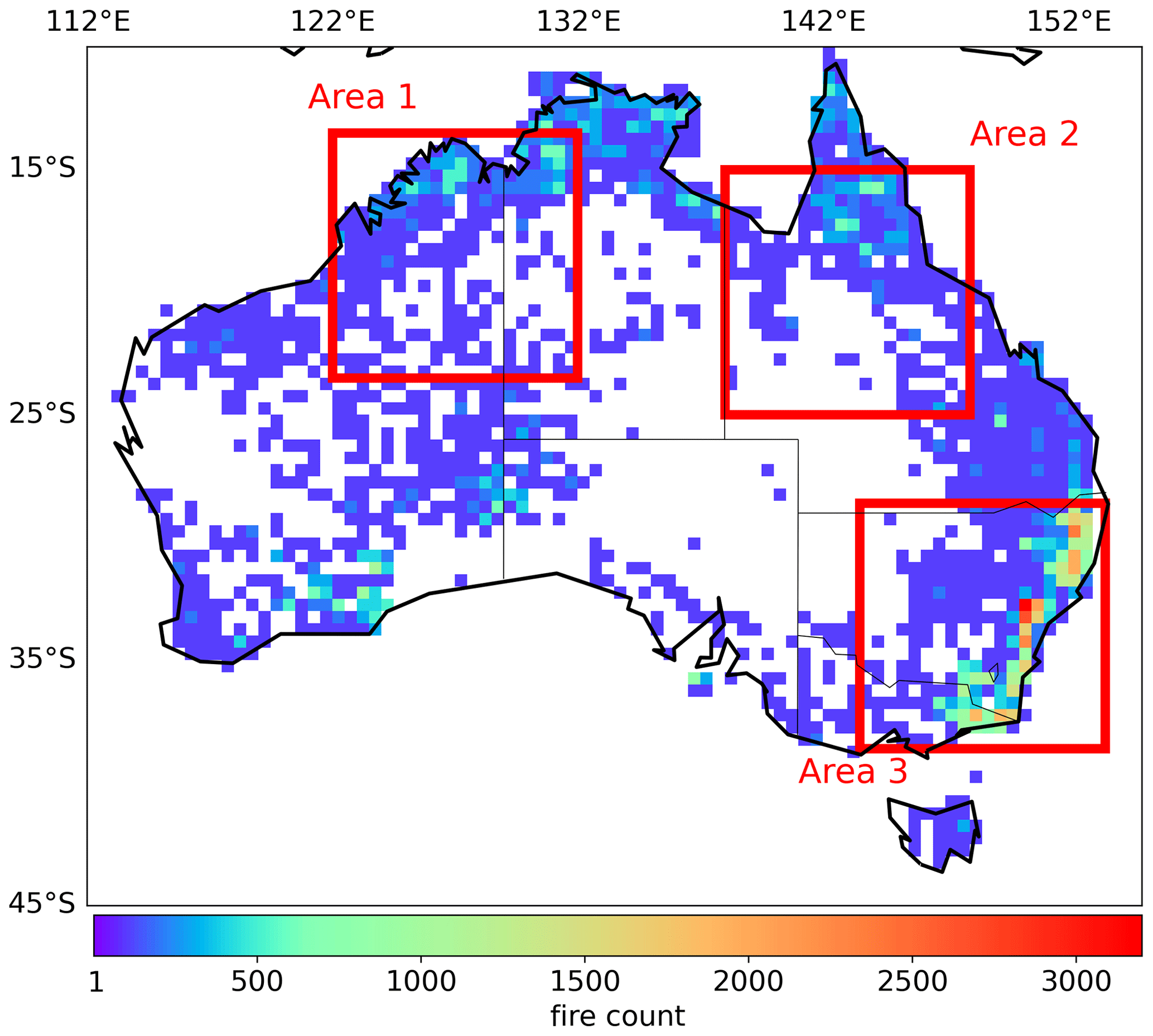
Figure 1Total fire counts from August 2019 through January 2020 at 0.5∘ × 0.5∘ resolution. Three 10∘ × 10∘ (latitude × longitude) areas indicate regions of interest in this study.
2.1 GFED4s database
The Global Fire Emission Database version 4 with small fires (GFED4s) provides global estimates of monthly and daily burned area, emissions, and fractional contributions of different fire types with 0.25∘ × 0.25∘ spatial resolution (Randerson et al., 2012). This database uses the Moderate Resolution Imaging Spectroradiometer (MODIS) Collection 5.1 MCD64A1 burned area product and includes small fires for emission estimates (Giglio et al., 2013). Six fuel classifications are estimated using the land cover type product from MODIS and the University of Maryland classification scheme in the GFED4s database, including temperate forest, boreal forest, deforested and degraded land, peatland, agricultural waste burning, and herbaceous fuel type, which is composed of shrubland, savanna, and grassland (Van der Werf et al., 2017). The vegetation fires that occurred in Australia from August 2019 through January 2020 were classified as savanna and temperate forest fires based on GFED4s. Highlighted in Fig. 1 are the three areas of interest employed in this study. The three selected areas include two savanna fire areas in northwestern (Area 1) and northeastern (Area 2) Australia, as well as an area with both savanna and temperate forest fires in southeastern (Area 3) Australia (Fig. 1). To be consistent for the three areas, we chose the same study period that covers all fires from August 2019 through January 2020.
2.2 TROPOMI CO, NO2, and fire plume data
The total column density of CO from TROPOMI was estimated from spectral radiance measurements from the shortwave to infrared spectral ranges around 2.3 µm that are sensitive to CO absorption with a daily 5.5 km × 7 km resolution (Landgraf et al., 2016; Borsdorff et al., 2018). Previous studies have shown that TROPOMI was able to capture the variability of daily CO as a result of atmospheric transport of pollution (Borsdorff et al., 2018; Schneising et al., 2020). The NO2 tropospheric column density is detected from TROPOMI's 405–465 nm wavelength bands with a 5.5 km × 3.5 km resolution. Although a negative bias exists of approximately 30 % in the lower tropospheric columns because of cloud pressure and the a priori NO2 profile used in air mass factor calculations (Lambert et al., 2018), it is still appropriate to use TROPOMI NO2 to quantify fire burning efficiency (Lama et al., 2019; Van der Velde et al., 2020). We chose an improved NO2 dataset from Van Geffen et al. (2022), which showed that, on average, the corrected NO2 tropospheric vertical column densities are 10 % to 40 % larger than the raw data, especially over large, polluted regions. Different algorithms are used to estimate NO2 and CO in TROPOMI channels, which also provide quality assurance values (i.e., QA value) to help filter raw data under unclear sky conditions and/or other problematic retrievals. In our study, we collected CO retrievals with a QA value larger than 0.5 and NO2 retrievals with a QA value larger than 0.75. The CO total column density and NO2 tropospheric column density were then converted to units of moles per square meter (mol m−2) and millimoles per square meter (mmol m−2), respectively. TROPOMI also provides aerosol layer height (ALH) data that are based on the O2 absorption band at near-infrared wavelengths (de Graaf et al., 2019). The ALH data were used to define the main vertical wind layer, which was required for the emission estimation procedure described in Sect. 3.2, and we added plume height data from the Global Fire Assimilation System (GFAS) as alternative values to use when ALH data were unavailable. All data were then resampled to 0.05∘ × 0.05∘ spatial resolution through an areal weighted interpolation using the Harp package from Python (Niemeijer, 2017).
2.3 MODIS fire radiative power (FRP) and fire events
The FRP represents the instantaneous radiative energy that is released from actively burning fires and is related to the rate of biomass combustion (Wooster et al., 2003), the emission rate of trace gases, and aerosol emissions (Kaiser et al., 2012). The MODIS instrument is on board both the Earth Observation System Terra and Aqua satellites of the National Aeronautics and Space Administration and measures radiance in spectral channels to detect fires at a 1 km spatial resolution (Kaufman et al., 1998). The MODIS near-real-time active fire product data (MCD14DL) were used to identify fire events from August 2019 through January 2020. For each day, fire pixels (i.e., 1 km × 1 km grid cells) located within a 20 km distance of one another were aggregated into a “fire event” forming a rectangular polygon with ± 50 km crosswind distance and 100 km downwind distance. The polygons were defined for the purpose of completing the emission calculation in Sect. 4.3. The fire event's center was set as the average latitude and longitude of all fire pixels weighted by each pixel's FRP, which is related to trace gas emission and widely used to estimate fire intensity (Wooster et al., 2003; Li et al., 2018). We retained only fire events for which the total FRP was larger than 200 MJ s−1 (megajoules per second). It should be noted that MODIS does not provide all fire event data due to cloudy days.
2.4 Wind
Wind fields, which include wind speed and direction, were obtained from the hourly ERA-5 reanalysis dataset from the European Centre for Medium-Range Weather Forecasts (ECMWF). This dataset provides meteorological variables for 37 vertical layers from 1000 to 1 hPa from 1979 to the present at 0.25∘ × 0.25∘ horizontal resolution (Hersbac et al., 2020). We first interpolated ERA-5 wind field data at TROPOMI overpass time (13:30 LT) and resampled to 0.05∘ × 0.05∘ resolution grids. Then, the data were vertically interpolated to the averaged ALH level within each fire event. For fire events without valid ALH data, the GFAS plume height data were used as a replacement. Otherwise, an average plume height over each area was used when both ALH and GFAS datasets were unavailable. The mean plume height was 822 hPa for Area 1, 866 hPa for Area 2, and 833 hPa for Area 3.
3.1 Emission ratio (ER)
Excess trace species concentration (ΔX) is defined as the difference between concentrations of species X in the fire plume (Xfire) and in the ambient background (Xbg). Usually, ΔX is divided by a reference species (ΔY), such as CO or CO2, to get the emission ratio (ER) between those two emitted compounds (i.e., . In our study, a local sampling method similar to that employed by Van der Velde et al. (2020) was used to calculate the ER. To calculate excess gas concentration over the three selected 10∘ × 10∘ areas (Fig. 1), daily TROPOMI data were first resampled into a 0.05∘ × 0.05∘ spatial resolution grid. Next, colocated NO2 and CO column densities from TROPOMI were obtained from locations where NOx and CO values were available from the GFED4s database in the three selected areas (Fig. 1). The Xfire plume value was calculated as the average of all selected column densities. The corresponding ambient background Xbg value was calculated as the average of all values inside a 5∘ × 5∘ subregion upwind of the biomass burning region but within the three 10∘ × 10∘ study areas. The upwind direction was determined by interpolating the surface daily ERA-5 wind data to the time and location of TROPOMI observations. The background subregions were determined by visual inspection through examining the predominant direction of the individual plume. Excess NO2 and CO concentrations were determined from the expressions ΔNO2 = − and ΔCO = COfire − CObg, respectively, and the emission ratio was thus calculated as . Days with inadequate data coverage (when the missing area exceeded 25 % of the selected area in a single day) in either the background or study areas were removed during computation. And the overall emission ratio for each area was calculated by averaging the daily emission ratios in the studied area. Although CO and NO2 also have strong anthropogenic sources, we minimized the influence of anthropogenic sources by selecting pixels colocated with FRP pixels.
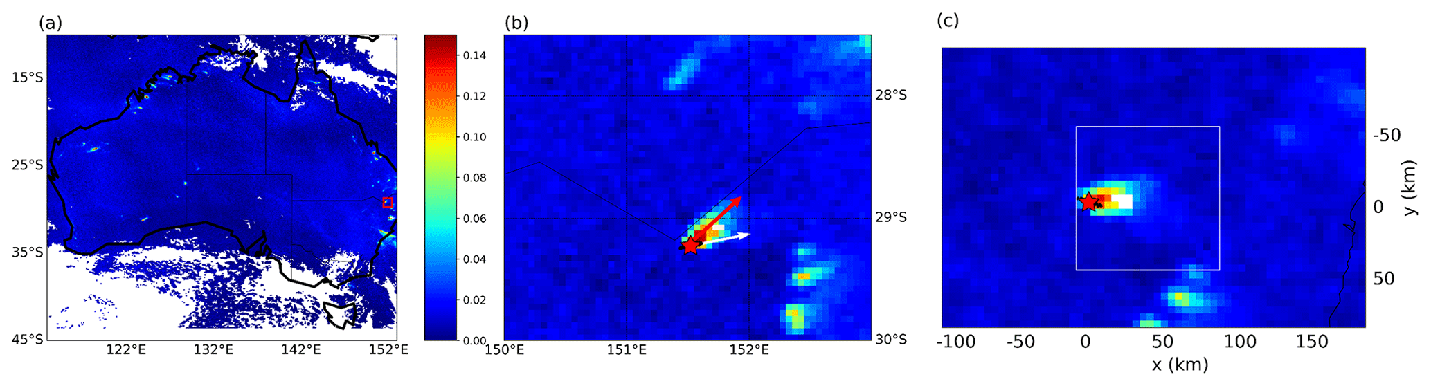
Figure 2An example of emission analysis for a fire event, with MODIS fire pixels indicated (black points) and the center of the fire event indicated by a red star. (a) Map of TROPOMI NO2 column density over Australia on 6 November 2019. The red box in southeastern Australia marks the fire event location. (b) The original TROPOMI NO2 column density with the wind direction is indicated by a white arrow. The red arrow indicates the plume direction. (c) The excess NO2 after (1) removing background column density from the original NO2 and (2) rotating all pixels examined to align with the wind direction; thus, a 20 km downwind distance area was selected and used to estimate the NO2 emission.
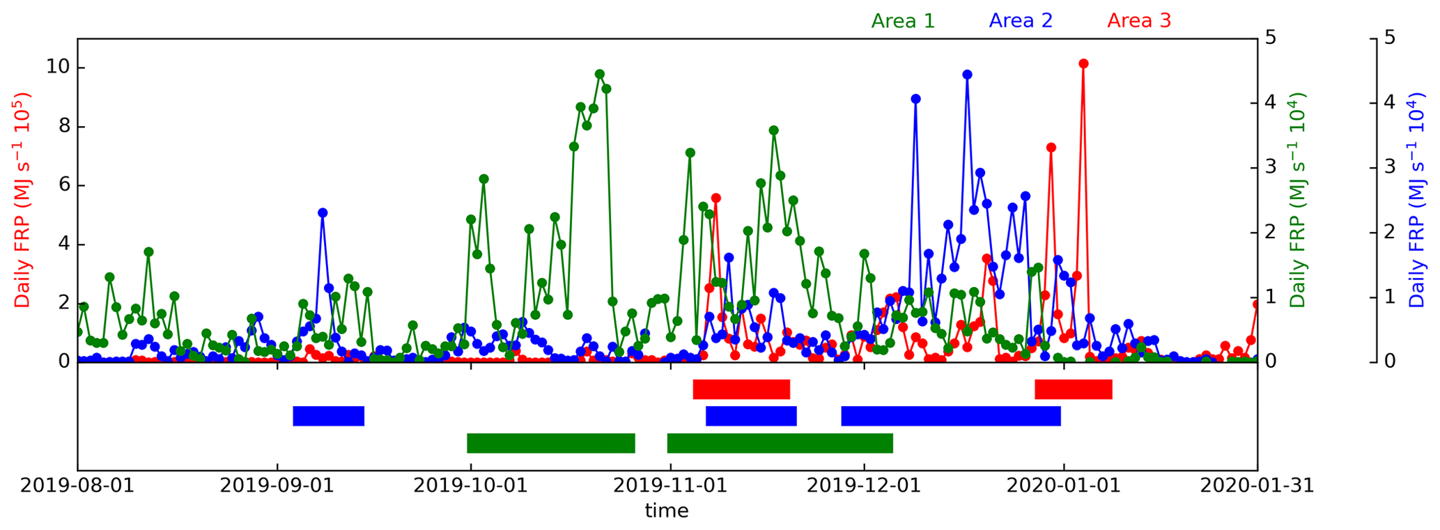
Figure 3Daily fire radiative power (FRP) from August 2019 through January 2020 for Area 1 (green), Area 2 (blue), and Area 3 (red). Several distinct periods are highlighted to show a significant increase in FRP, covering 1–24 October and 1 November to 3 December (Area 1), 4–13 September (Area 2), 7–18 November and 28 November to 29 December (Area 2), 5–17 November (Area 3), and 28 December to 6 January (Area 3).
3.2 Emissions from satellite measurement and emission factor (EF)
In our study, downwind flux was estimated using an integrated mass enhancement method that has been used in previous studies (Mebust et al., 2011; Adams et al., 2019; Griffin et al., 2021). Since the 2018–2019 fire events in Areas 1 and 2 were larger than those in 2020–2021, the period from August 2020 through January 2021 was used as the background data for both CO and NO2 column densities to represent emissions under less intense fire conditions. To improve background robustness for daily gas column density, we removed raw column density values that were above the 99th percentile on each day in each area, then refilled back by interpolation using the nearest neighboring data. The means and standard deviations of the background data indicated that the background selected did not have a strong systematic variation. The background values for CO ranged from 0.018 ± 0.001 to 0.032 ± 0.002 mol m−2, and the background values for NO2 ranged from 0.007 ± 0.002 to 0.011 ± 0.005 mmol m−2. The daily column density was then calculated by subtracting corresponding monthly background values from raw daily column density values. When estimating CO and NO2 emission from biomass burning, we excluded the TROPOMI dataset over the areas with pyrocumulus (PyroCb) events between 29–31 December 2019 and 4 January 2020 based on the PyroCb activity dataset of Peterson et al. (2021) because the flux method should be used under no PyroCb development condition (Griffin et al., 2021). Fire pixels were grouped based on distance as described in Sect. 2.3, and surrounding rectangles were defined. The total mass, m (g), emitted by fires is the product of daily column density and area (Eq. 1):
where VCD (mol m−2) is the daily vertical column density after subtracting background values, and A is the rectangle area (m2). A line density derived from a Gaussian model of a plume traveling downwind under assumptions of constant wind without diffusion and deposition (Adams et al., 2019) is expressed as Eq. (2):
where L0 (mol m−1) is the concentration over the fire center calculated by integrating VCD (mol m−2) from ± 50 km crosswind direction, the lifetime τ is the inverse of reaction rate coefficient k (), and t is the time for emitted gas transport from the fire center to downwind distance x. μ is averaged wind speed at the mean ALH level in the rectangle. L(x) (mol m−1) is the line density at x downwind distance. The total mass m also equals the integral of gas density from the fire center to x distance (Eq. 3):
Therefore, is the residence time inside the areas from the fire center to downwind distance x. L0xt−1 equals the emission rate E (g s−1). The relationship between total mass and the emission rate can be expressed as
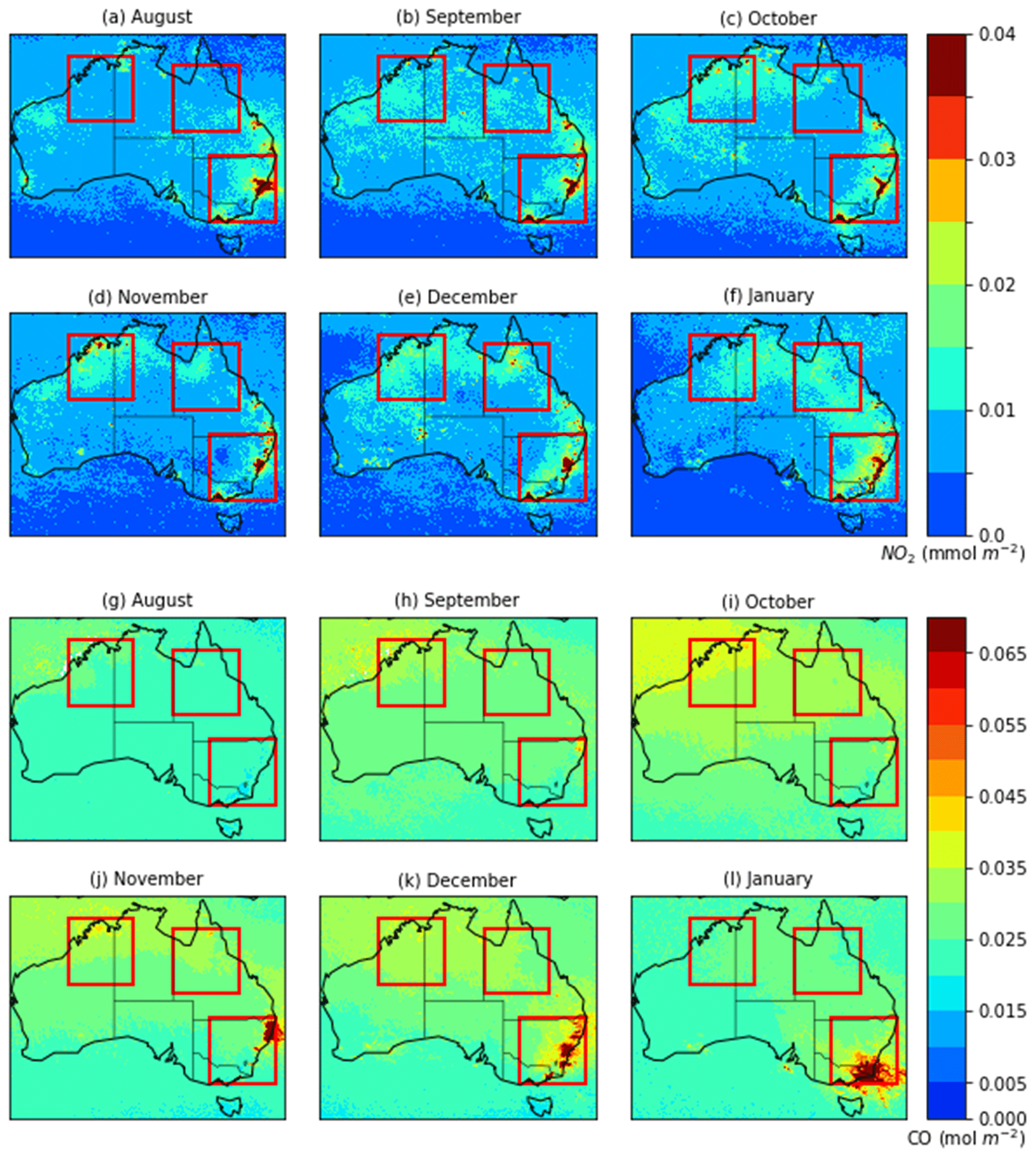
Figure 4Monthly average NO2 (a–f) and CO (g–l) column density from August 2019 through January 2020. Three 10∘ × 10∘ (latitude × longitude) areas indicate regions of interest in this study.
In this study, the downwind distance x was set as 20 km based on previous studies (Adams et al., 2019; Griffin et al., 2021), and therefore the area in Eq. (1) is the area of 20 km downwind distance. We used Eq. (4) to estimate the emission rate with constant wind and estimated lifetime by using Eq. (2). Figure 2a–c show an example of calculating emission for a fire event that occurred within Area 3 of southeastern Australia (29.2∘ S, 151.5∘ E) on 6 November 2019. The red box (Fig. 2a) and white box (Fig. 2c) show the area within which the FRP fire pixels were grouped and TROPOMI data background column density values were removed. The location for the center of the fire was set at the averaged latitude and longitude of all fire pixels (the red star), and then the mean wind direction was calculated. Lastly, the TROPOMI data plume direction (red arrow) was rotated to align with the wind direction. We derived CO and NO2 emission flux in grams per second (g s−1) based on Eq. (4), and an ratio of 0.75 was used to convert NO2 to NOx. Previous studies (Yurganov et al., 2011; R'Honi et al., 2013; Whitburn et al., 2015) indicated a 7 d or 14 d effective lifetime for CO, so a 7 d effective lifetime was used in our study determined through a sensitivity test discussed in Sect. 4.3. For the short-lifetime NO2, Mebust et al. (2011) assumed a 2 h effective lifetime based on the fitted lifetimes from the OMI tropospheric NO2 columns, whereas Tanimoto et al. (2015) used 2 or 6 h as the effective lifetimes. In our study, Eq. (2) was used to estimate the NO2 lifetime by fitting an exponential to L(x) as a function of downwind distance and wind speed. Finally, we used the emission coefficient (g MJ−1), an energy-based coefficient, which is defined as the mass of pollutants emitted per unit of radiative energy. The emission coefficient was estimated as the slope of the linear relationship between emission estimates and FRP, with an intercept fixed at zero (Vermote et al., 2009). For both savanna and temperate forest fires, we converted regression emission coefficients to EFs using an energy-to-mass factor of 0.41 ± 0.04 kg MJ−1, which is the average of the 0.368 ± 0.015 and 0.453 ± 0.068 kg MJ−1 values reported by others (Wooster et al., 2005; Freeborn et al., 2008; Vermote et al., 2009). It should be noted that recirculating plumes have not been taken into account in our analysis, which may cause some degree of uncertainty in our emission ratio estimates.
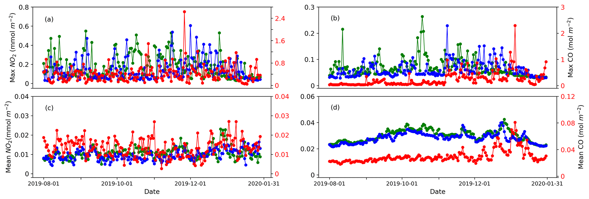
Figure 5Time series of daily maximum NO2 (a) and CO (b) total column densities from August 2019 through January 2020 as well as daily mean NO2 (c) and CO (d) for three highlighted areas: Area 1 (green), Area 2 (blue), and Area 3 (red). Results for Areas 1 and 2 are displayed by the left Y axis, and results for Area 3 are displayed in red on the right Y axis.

Figure 6The relationship between daily ΔCO (mol m−2) and daily ΔNO2 (mmol m−2) in savanna regions (a for Area 1, b for Area 2, and c for Area 3) and temperate forest regions (d for Area 3 only). The color bars are coded by daily FRP; data points with black edges are the days with high FRP (highlighted periods) in Fig. 4. The blue markers represent the monthly average relationship between ΔCO and ΔNO2 with day-to-day variabilities represented by the error bars. ER stands for the total emission ratio expressed by overall mean plus and minus 1 standard deviation.
4.1 Temporal evolution of fire intensity and total column density
The majority of fire-affected regions during these extreme fire events were located in Area 3 in southeastern Australia (Fig. 1) where the largest cumulative fire counts exceeded 1000. Fire frequencies were much lower in Areas 1 and 2 where the largest cumulative fire counts did not exceed 700. The fire-affected areas were dominantly located either in far northern oceanic boundaries of Areas 1 and 2 or in the southeastern oceanic boundary of Area 3 (Fig. 1). From the fire data product of MCD14DL, the daily FRP observations showed a few distinct periods of peak fire events (Fig. 3), including 3 weeks from 1 to 24 October and 4 weeks from 1 November to 3 December in Area 1, as well as 3 weeks for Area 2 from 28 November to 29 December. For Area 3, there were two short FRP peaks in November and early January. The highest FRPs during these periods of peak fire events were 4.45 × 10⁴, 4.44 × 10⁴, and 1.01 × 10⁶ MJ s−1 for Areas 1, 2, and 3, respectively. The most intensive fire events were observed in October and November 2019 for Area 1, in December 2019 for Area 2, and in January 2020 for Area 3 (Fig. 3). Within these 6 months, both NO2 and CO column density distributions showed a larger mean value for each month over Area 3 compared to the other two study regions (Fig. 4). These higher NO2 and CO column density observations reflect the larger FRP over Area 3 (Figs. 3 and 4). As expected, the daily maximum NO2 column density in Area 3 was nearly double that of the other two areas (Fig. 5a), but their mean values were comparable (Fig. 5c), indicating highly fluctuated NO2 densities on a fire day. On the other hand, daily maximum CO column density was nearly 10 times higher in Area 3 than those estimated for Areas 1 and 2 (Fig. 5b), suggesting the role of different fuel and fire combustion types. The maximum daily column densities were observed as 1.26 mmol m−2 for NO2 on 28 November and 2.3 mol m−2 for CO on 4 January in Area 3. For the daily mean total column densities, both NO2 and CO are significantly different for all three areas under the two-sample t test. Again, the daily mean CO was more sensitive to the FRP compared to NO2 (Fig. 5d). In addition, significant increases in CO and NO2 mean values in Area 3 were observed in early January, which was certainly associated with the large FRP values that were detected on 30 December 2019 and 4 January 2020 (Fig. 3) by MODIS satellites.
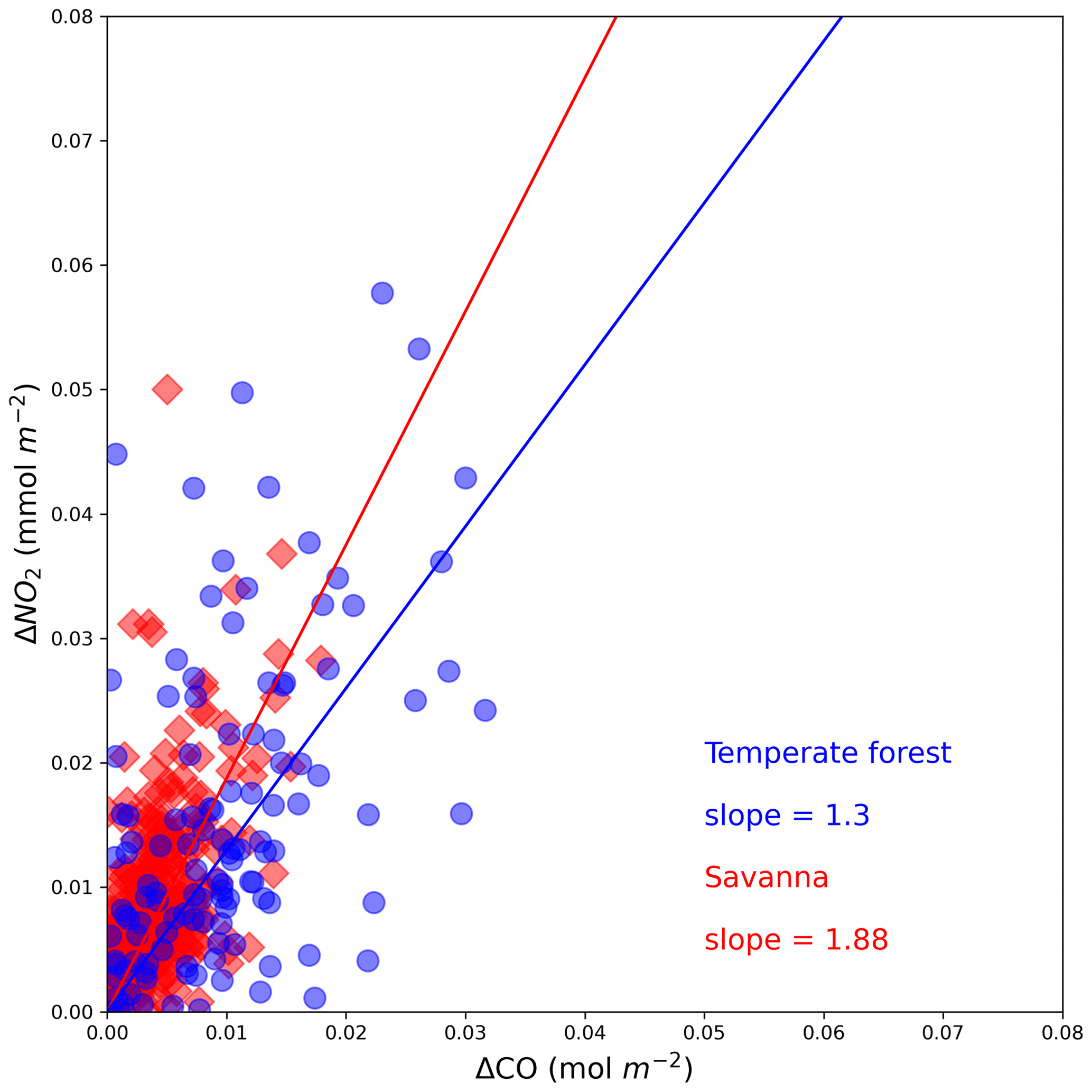
Figure 7The relationship between daily ΔCO (mol m−2) and daily ΔNO2 (mmol m−2) was derived from TROPOMI for all regions. The slope of linear fit with an intercept at zero represents the combustion efficiency of different fire types.
4.2 Emission ratio (ER) in savanna and temperate forest
Different from the calculation of gas concentrations, the excess gas concentration (expressed as ΔX) is derived by removing the impact of potentially varying amounts of background concentration and thus represents the gas emissions related to fire activities. The averaged ERs derived from savanna fires were 2.34, 2.60, and 2.03 for Areas 1, 2, and 3, respectively. The ER for temperate forests in Area 3 was, on average, 1.57 during the 6 months of this study period (Fig. 6). As expected, ΔNO2 and ΔCO both increased with increasing FRP (high FRP periods were highlighted in Fig. 3 to correspond to points with black edge markers shown in Fig. 6) for both savanna and temperate-forest-dominated landscapes, but there was a clear distinction between savanna and temperate forest fires. For the savanna fires, ΔNO2 approached 0.05 mmol m−2, whereas changes in ΔCO were much less at 0.03 mol m−2 across all three study areas. However, ΔNO2 (up to 0.08 mol m−2) and ΔCO (up to 0.08 mol m−2) for temperate forest fires in Area 3 were both larger in magnitude and variability. ΔCO and ΔNO2 emissions in temperate forest regions showed a larger enhancement compared to savanna fires. The ΔNO2 and ΔCO in temperate forests exceeded those in savanna fires within the same region because temperate forest fuels consisted mainly of eucalyptus trees (Godfree et al., 2021). The relatively high ΔNO2 and small ΔCO in the savanna portion of the three burning areas showed that the flaming combustion phase was dominant in savanna fires as this phase tends to produce higher NO2 as previous research has shown (Andreae and Merlet, 2001). The day-to-day variability in ΔNO2 was larger than the day-to-day variability in ΔCO. The ΔCO emission ranged from 0 to 0.08 mol m−2, whereas ΔNO2 emission ranged from 0 to 0.08 mmol m−2. Compared to the result of Van der Velde et al. (2020), who estimated ERs between 3.58 and 6.2 for savanna fires, the ER values in our study were lower and ranged between 2 and 2.8. The ER for temperate forest combustion reported here (1.5) was also lower than the results from Young and Paton-Walsh (2011), which was 5 ± 2 mmol mol−1, suggesting a complex interaction between dominant vegetation and local atmospheric turbulence during fire events. Although there are uncertainties from TROPOMI, there were distinct ERs clearly resulting from savanna and temperate forest combustion (Fig. 7). This result suggests that temperate forest fires emitted larger CO per unit NO2 compared to savanna fires, indicating less efficient combustion in temperate forest fires than in savanna fires (Fig. 7).
One possible reason for different ER values was the different land surface sensitivities of TROPOMI in CO and NO2 measurements (Val Martin et al., 2018; Van der Velde et al., 2020). Previous studies have shown that tropospheric NO2 measurement was less sensitive to sources in the planetary boundary layer than CO measurements, which causes underestimation of ΔNO2 (Borsdorff et al., 2018; Van der Velde et al., 2020). A second reason is the highly reactive property of NO2. The short lifetime of NO2 makes the daily values underestimated compared to CO, which has a relatively long lifetime. In addition, the natural variability of atmospheric composition (e.g., tropospheric O3, water vapor) and different measurement techniques may contribute to the measurement uncertainty.
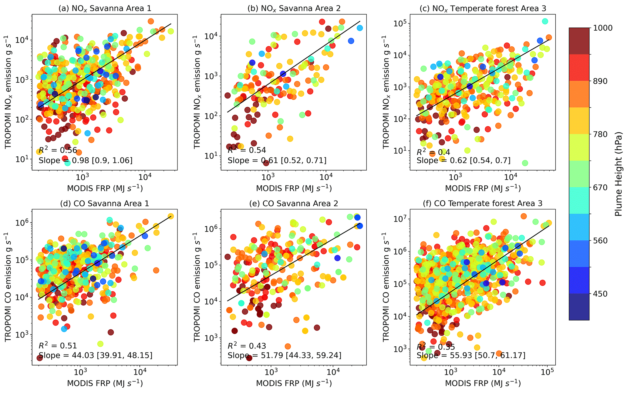
Figure 8Scatter plots of TROPOMI-derived NOx and CO emissions (g s−1) versus MODIS FRP in savanna regions (a, d for Area 1, b, e for Area 2) and temperate forest regions (c, f for Area 3). The black line indicates the regression line estimated from ordinary least squares regression with the intercept fixed at zero. Slopes are shown with a 95 % confidence interval. The color represents the plume height of the corresponding fire events. Emissions and FRP are on log scales.
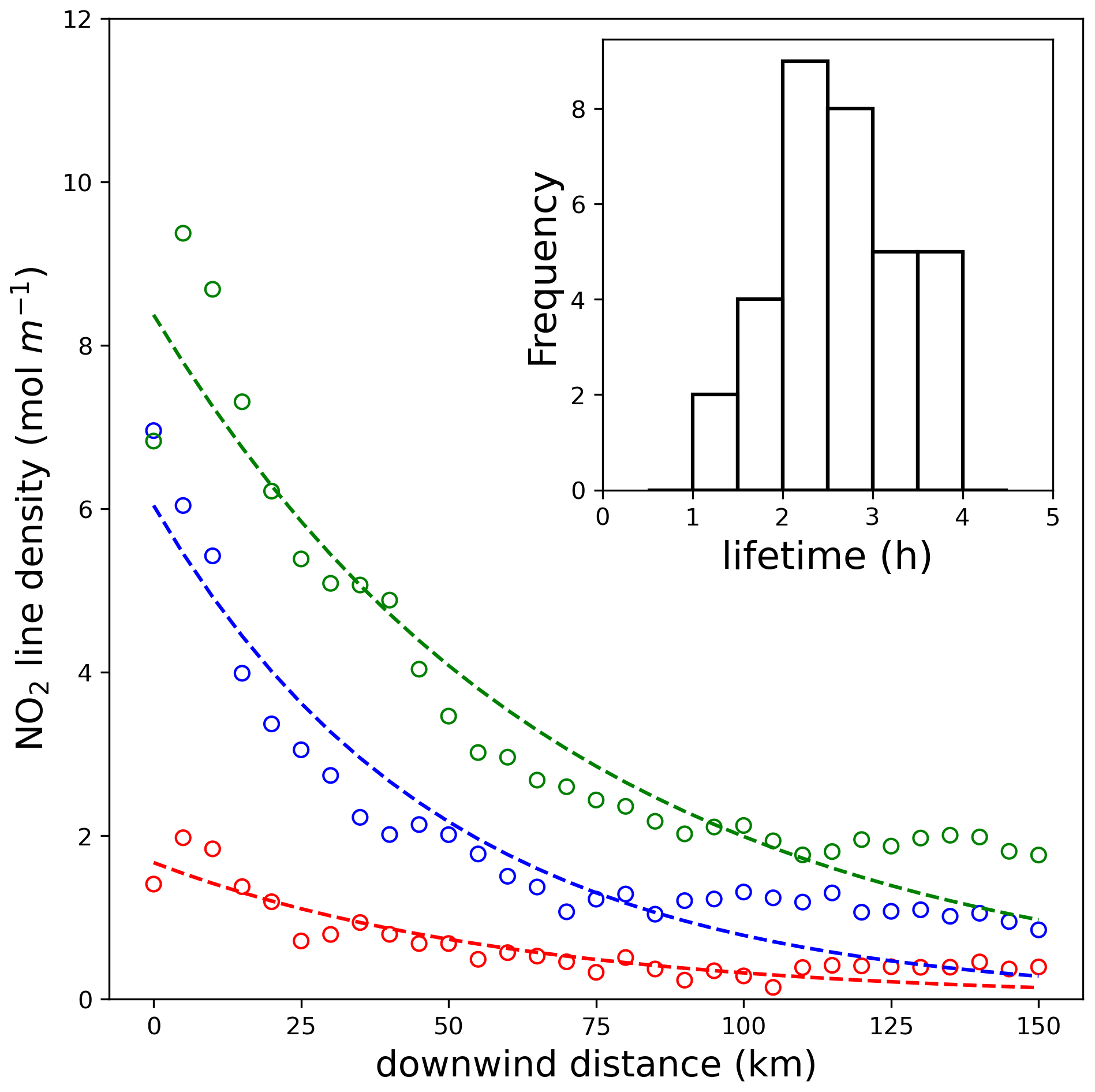
Figure 9NO2 line density decay curves of three example fire events (each color represents a fire event) in Area 2. The embedded histogram shows the frequency distribution of NO2 lifetime estimated from all three areas.
4.3 Satellite-derived emission factor (EF)
After deriving the NO2 and CO emissions for fire events, we calculated the emission coefficient (g MJ−1) using satellite-derived emissions and FRP. The 95 % confidence intervals of the slope were computed based on the Student's t-distribution test. Figure 8 shows the relationship between TROPOMI-derived NOx, CO emissions, and MODIS FRP for savanna and temperate forest fires in three areas. The FRP explains 40 % to 56 % variance in NOx emissions with the highest R2 in temperate fires in Area 3 and lowest in savanna fires in Area 1. For CO emission, the FRP explained 35 % to 51 % variance with the highest R2 in savanna fires and the lowest in temperate fires. The variability may relate to multiple uncertainties including the satellite retrieval and emission estimate approach, as we discussed below. Comparing different fire types, the NOx emission coefficient in savanna fires in Area 1 is the largest (0.98 g MJ−1), with 95 % confidence intervals of 0.9–1.06 g MJ−1, and the CO emission coefficient in temperate forest fires in Area 3 is the largest (55.93 g MJ−1), with 95 % confidence intervals of 50.7–61.17 g MJ−1.
To compare with previous studies, we converted emission coefficients to EFs by applying a conversion factor (Vermote et al., 2009). For NOx, the satellite-derived EFs range from 1.48 to 2.39 g kg−1 in savanna fires, which are slightly lower than the value 2.49 g kg−1 of Jin et al. (2021), who used TROPOMI NO2 data with updating a priori profile, and the values 2.5 ± 1.3 g kg−1 from Andreae (2019) that represent an updated compilation of EFs over the past 20 years. For temperate forests, the satellite-derived is 1.51 g kg−1, which is also less than the value 3 g kg−1 of Andreae (2019). For CO, the satellite-derived EFCO in savanna fires ranges from 107.39 to 126.32 g kg−1 and those values are larger than the values 69 ± 20 g kg−1 of Andreae (2019) but in the range of the field measurements (ranging 15 to 147 g kg−1) from the SAFIRED campaign savanna fires in Australia (Desservettaz et al., 2017). Our satellite-derived EFCO in temperate forest fires is 136.41 g kg−1, which is close to the value 113 ± 50 g kg−1 of Andreae (2019) and the field measurements of Guérette et al. (2018), which ranged from 101 to 118 g kg−1 in Australia temperate forest fires.
Our NOx EFs are smaller than those reported in previous studies, while CO EFs are the opposite. One source of this variance is because of aerosol smoke impact on the CO and NO2 volume column density retrieval process. Hirsch and Koren (2021) found that unprecedented bushfires in Australia caused record-breaking levels of aerosols, as TROPOMI CO values were monitored using radiances in the shortwave infrared bands so that the smoke aerosol does not have a strong effect on measurements. Schneising et al. (2020) show that the uncertainty due to smoke aerosol during several Californian wildfires was about 5 %. However, smoke aerosols have always affected TROPOMI NO2 observations in the ultraviolet–visible region when estimating fire emissions. Previous studies showed that an implicit aerosol correction can be applied to retrieval algorithms (Griffin et al., 2021), and without this correction, a bias of more than 40 % over polluted regions could be introduced (Lorente et al., 2017), suggesting that the estimated daily CO net emission was much more accurate than the estimated NO2 emissions. The uncertainty in the satellite emission method (e.g., the lifetime used in emission estimation) can also be a cause of variance. Figure 9 shows an example of fits for NO2 in Area 2, and the embedded histogram shows the frequency distribution of NO2 lifetime ranging from 1 to 4 h over all three areas. Thus, an average of 2.5 h for NO2 selected in our computation was optimal for calculating emission. To test the uncertainty related to different lifetime choices, the Adams et al. (2019) test was followed. Fluxes were recalculated by replacing the default lifetime ( h, τCO = 7 d) with alternate lifetimes ( h, h, and d), and then the percent differences between EFs were calculated. The largest deviation from the default settings was defined as the uncertainty (Adams et al., 2019). For CO, the uncertainty based on the 14 d lifetime was smaller (less than 1 %), whereas the uncertainty based on the largest 4 h lifetime was larger for NO2 (37 % in savanna fires in Area 1).
The 2019–2020 black summer fires in Australia emitted large quantities of trace gases and aerosols. In this study, we focused on the analysis of two trace gases: CO and NO2. Based on the total columns (mean and maximum) from TROPOMI observations and the fire intensity from MODIS in late 2019 to early 2020, we estimated the ERs of NO2 relative to CO for each day over three selected areas with savanna and temperate forest vegetation. For temperate forest fires, the ER was 1.57 ± 1.71, which is consistent with previous studies. For savanna vegetation fires, the ER ranged from 2.0 ± 2.36 to 2.6 ± 1.92, which is slightly lower compared to other studies. These differences could be traced back to different measurement techniques used, their spatial resolutions, nonlinear sensitivities to gas densities in the boundary layer, and larger NO2 natural variability due to its short lifetime, all of which suggest that further validation of satellite products and investigations of more cases are required. For example, aircraft measurements from NASA airborne campaigns could be used to validate TROPOMI satellite-derived CO and NO2 concentrations. The satellite-derived concentrations and emission estimates could also be compared with simulations from dynamical models (e.g., Weather Research and Forecasting model coupled to Chemistry, Community Modeling and Analysis System). Further advanced techniques to improve the calibration and retrieval algorithm could be used to improve the estimates of emissions and emission factors. For instance, even though we used the improved TROPOMI NO2 data from Van Geffen et al. (2022) in this study, they still have a negative bias when compared with ground-based observations, which probably is due to the relatively coarse resolution (1∘ × 1∘) of the a priori profiles used. Taking advantage of higher-resolution profile shapes can lead to better retrieval of tropospheric columns over emission hotspots (Douros et al., 2022). Additionally, considering the short lifetime of NO2, the NO2 tropospheric column could be corrected using boundary layer temperature and OH concentration, as described in the work of Lama et al. (2019)
Using the methods from Mebust et al. (2011) and Adams et al. (2019), net emission fluxes were estimated by using a 14 d CO effective lifetime and a 2.5 h NO2 effective lifetime, and EFs were calculated. The TROPOMI-derived NOx EFs were 1.48 and 1.51 g kg−1 for savanna and temperate forest fires, respectively, which are lower than previous studies, while the CO EFs were 107.39 g kg−1 for savanna fires and 136.41 g kg−1 for the temperate forest. Our study on both savanna and temperate forest fire emissions demonstrates the capability and limitations of TROPOMI data for the study of the regional variability of combustion characteristics and their impacts on regional atmospheric composition and air quality. Benefiting from the global coverage of TROPOMI and its high spatial resolution, the method used in our study could be applied to different vegetation wildfires at various scales, even the burning of fossil fuel in megacities.
The TROPOMI CO data (https://doi.org/10.5270/S5P-bj3nry0, Copernicus Sentinel-5P, 2021) and TROPOMI ALH (https://doi.org/10.5270/S5P-j7aj4gr, Copernicus Sentinel-5P, 2018) are available from NASA Goddard Earth Sciences (GES). TROPOMI NO2 is available via the S5P-PAL Data Portal (https://data-portal.s5p-pal.com/, last access date: 22 December 2022). The GFAS fire plume data are available from the Copernicus Atmosphere Monitoring Service (CAMS) (http://apps.ecmwf.int/datasets/, last access: 22 December 2022, GFAS, 2019). MODIS FRP data are available from NASA Earth Data Fire Information for Resource Management Systems (https://doi.org/10.5067/FIRMS/MODIS/MCD14ML, NASA FIRMS, 2018). ERA5 wind data are available from the Copernicus Climate Service (C3S) Climate Data Store (available at https://doi.org/10.24381/cds.bd0915c6, Hersbach et al., 2018).
NW worked on the emission estimate methodology. HZ helped to interpret the satellite datasets. XX and XL conceived the structure of the paper. NW prepared the paper, and all authors contributed to the discussion and revision of the paper.
The contact author has declared that none of the authors has any competing interests.
Publisher's note: Copernicus Publications remains neutral with regard to jurisdictional claims in published maps and institutional affiliations.
The contribution number of this paper is 22-275-J. We thank Dallas Staley for her outstanding contribution in editing and finalizing an earlier version of the paper. Her work continues to be at the highest professional level.
This research has been supported by the U.S. Department of Agriculture (grant no. 2016-68007-25066).
This paper was edited by Bryan N. Duncan and reviewed by two anonymous referees.
Abram, N. J., Henley, B. J., Sen Gupta, A., Lippmann, T. J. R., Clarke, H., Dowdy, A. J., Sharples, J. J., Nolan, R. H., Zhang, T., Wooster, M. J., Wurtzel, J. B., Meissner, K. J., Pitman, A. J., Ukkola, A. M., Murphy, B. P., Tapper, N. J., and Boer, M. M.: Connections of climate change and variability to large and extreme forest fires in southeast Australia, Commun. Earth Environ., 2, 8, https://doi.org/10.1038/s43247-020-00065-8, 2021.
Adams, C., McLinden, C. A., Shephard, M. W., Dickson, N., Dammers, E., Chen, J., Makar, P., Cady-Pereira, K. E., Tam, N., Kharol, S. K., Lamsal, L. N., and Krotkov, N. A.: Satellite-derived emissions of carbon monoxide, ammonia, and nitrogen dioxide from the 2016 Horse River wildfire in the Fort McMurray area, Atmos. Chem. Phys., 19, 2577–2599, https://doi.org/10.5194/acp-19-2577-2019, 2019.
Andreae, M. O.: Emission of trace gases and aerosols from biomass burning – an updated assessment, Atmos. Chem. Phys., 19, 8523–8546, https://doi.org/10.5194/acp-19-8523-2019, 2019.
Andreae, M. O. and Merlet, P.: Emission of trace gases and aerosols from biomass burning, Global Biogeochem. Cy., 15, 955–966, https://doi.org/10.1029/2000GB001382, 2001.
Boer, M. M., Resco de Dios, V., and Bradstock, R. A.: Unprecedented burn area of Australian mega forest fires, Nat. Clim. Change., 10, 171–172, https://doi.org/10.1038/s41558-020-0716-1, 2020.
Borchers A., N., Palmer, A. J., Bowman, D. M., Morgan, G. G., Jalaludin, B. B., and Johnston, F. H.: Unprecedented smoke-related health burden associated with the 2019–20 bushfires in eastern Australia, Med. J. Aust., 213, 282–283, https://doi.org/10.5694/mja2.50545, 2020.
Borsdorff, T., aan de Brugh, J., Hu, H., Hasekamp, O., Sussmann, R., Rettinger, M., Hase, F., Gross, J., Schneider, M., Garcia, O., Stremme, W., Grutter, M., Feist, D. G., Arnold, S. G., De Mazière, M., Kumar Sha, M., Pollard, D. F., Kiel, M., Roehl, C., Wennberg, P. O., Toon, G. C., and Landgraf, J.: Mapping carbon monoxide pollution from space down to city scales with daily global coverage, Atmos. Meas. Tech., 11, 5507–5518, https://doi.org/10.5194/amt-11-5507-2018, 2018.
Bowman, D. M. J. S., Williamson, G. J., Abatzoglou, J. T., Kolden, C. A., Cochrane, M. A., and Smith, A. M. S.: Human exposure and sensitivity to globally extreme wildfire events, Nat. Ecol. Evol., 1, 0058, https://doi.org/10.1038/s41559-016-0058, 2017.
Cai, W., Cowan, T., and Raupach, M.: Positive Indian Ocean Dipole events precondition southeast Australia bushfires, Geophys. Res. Lett., 36, L19710, https://doi.org/10.1029/2009GL039902, 2009.
Copernicus Sentinel-5P (processed by ESA): TROPOMI Level 2 Aerosol Layer Height products, Version 01, European Space Agency [data set], https://doi.org/10.5270/S5P-j7aj4gr, 2018.
Copernicus Sentinel-5P (processed by ESA): TROPOMI Level 2 Carbon Monoxide total column products, Version 02, European Space Agency [data set], https://doi.org/10.5270/S5P-bj3nry0, 2021.
de Graaf, M., de Haan, J. F., and Sanders, A. F. J.: TROPOMI ATBD of the Aerosol Layer Height, S5P-KNMI-L2-0006-RP, http://www.tropomi.eu/sites/default/files/files/publicSentinel-5P-TROPOMI-ATBD-Aerosol-Height.pdf (last access: January 2020), 2019.
Desservettaz, M., Paton-Walsh, C., Griffith, D. W. T., Kettlewell, G., Keywood, M. D., Vanderschoot, M. V., Ward, J., Mallet, M. D., Milic, A., Miljevic, B., Ristovski, Z. D., Howard, D., Edwards, G. C., and Atkinson, B.: Emission factors of trace gases and particles from tropical savanna fires in Australia, J. Geophys. Res.-Atmos., 122, 6059–6074, https://doi.org/10.1002/2016JD025925, 2017.
Douros, J., Eskes, H., van Geffen, J., Boersma, K. F., Compernolle, S., Pinardi, G., Blechschmidt, A.-M., Peuch, V.-H., Colette, A., and Veefkind, P.: Comparing Sentinel-5P TROPOMI NO2 column observations with the CAMS-regional air quality ensemble, EGUsphere [preprint], https://doi.org/10.5194/egusphere-2022-365, 2022.
Filkov, A. I., Ngo, T., Matthews, S., Telfer, S., and Penman, T. D.: Impact of Australia's catastrophic 2019/20 bushfire season on communities and environment. Retrospective analysis and current trends, Journal of Safety Science and Resilience, 1, 44–56, https://doi.org/10.1016/j.jnlssr.2020.06.009, 2020.
Fowler, D., Amann, M., Anderson, R., Ashmore, M., Cox, P., Depledge, M., Derwent, D., Grennfelt, P., Hewitt, N., Hov, O., Jenkin, M., Kelly, F., Liss, P., Pilling, M., Pyle, J., Slingo, J., and Stevenson, D.: Ground-level ozone in the 21st century: future trends, impacts and policy implications, The Royal Society, ISBN 978-0-85403-713-1301, 2008.
Freeborn, P. H., Wooster, M. J., Hao, W. M., Ryan, C. A., Nordgren, B. L., Baker, S. P., and Ichoku, C.: Relationships between energy release, fuel mass loss, and trace gas and aerosol emissions during laboratory biomass fires, J. Geophys. Res.-Atmos., 113, D01301, https://doi.org/10.1029/2007JD008679, 2008.
Giglio, L., Randerson, J. T., and van der Werf, G. R.: Analysis of daily, monthly, and annual burned area using the fourth-generation global fire emissions database (GFED4), J. Geophys. Res.-Biogeosci., 118, 317–328, https://doi.org/10.1002/jgrg.20042, 2013.
Global Fire Assimilation System (GFAS): CAMS GFAS Output, [data set], http://apps.ecmwf.int/datasets/ (last access: 22 December 2022), 2019.
Godfree, R. C., Knerr, N., Encinas-Viso, F., Albrecht, D., Bush, D., Cargill, D. C., Clements, M., Gueidan, C., Guja, L. K., Harwood, T., Joseph, L., Lepschi, B., Nargar, K., Schmidt-Lebuhn, A., and Broadhurst, L. M.: Implications of the 2019–2020 megafires for the biogeography and conservation of Australian vegetation, Nat. Commun., 12, 1023, https://doi.org/10.1038/s41467-021-21266-5, 2021.
Griffin, D., McLinden, C. A., Dammers, E., Adams, C., Stockwell, C. E., Warneke, C., Bourgeois, I., Peischl, J., Ryerson, T. B., Zarzana, K. J., Rowe, J. P., Volkamer, R., Knote, C., Kille, N., Koenig, T. K., Lee, C. F., Rollins, D., Rickly, P. S., Chen, J., Fehr, L., Bourassa, A., Degenstein, D., Hayden, K., Mihele, C., Wren, S. N., Liggio, J., Akingunola, A., and Makar, P.: Biomass burning nitrogen dioxide emissions derived from space with TROPOMI: methodology and validation, Atmos. Meas. Tech., 14, 7929–7957, https://doi.org/10.5194/amt-14-7929-2021, 2021.
Guérette, E.-A., Paton-Walsh, C., Desservettaz, M., Smith, T. E. L., Volkova, L., Weston, C. J., and Meyer, C. P.: Emissions of trace gases from Australian temperate forest fires: emission factors and dependence on modified combustion efficiency, Atmos. Chem. Phys., 18, 3717–3735, https://doi.org/10.5194/acp-18-3717-2018, 2018.
Hersbach, H., Bell, B., Berrisford, P., Biavati, G., Horányi, A., Muñoz Sabater, J., Nicolas, J., Peubey, C., Radu, R., Rozum, I., Schepers, D., Simmons, A., Soci, C., Dee, D., and Thépaut, J-N.: ERA5 hourly data on pressure levels from 1959 to present, Copernicus Climate Change Service (C3S) Climate Data Store (CDS) [data set], https://doi.org/10.24381/cds.bd0915c6, 2018.
Hersbach, H., Bell, B., Berrisford, P., Hirahara, S., Horányi, A., Muñoz-Sabater, J., Nicolas, J., Peubey, C., Radu, R., Schepers, D., Simmons, A., Soci, C., Abdalla, S., Abellan, X., Balsamo, G., Bechtold, P., Biavati, G., Bidlot, J., Bonavita, M., De Chiara, G., Dahlgren, P., Dee, D., Diamantakis, M., Dragani, R., Flemming, J., Forbes, R., Fuentes, M., Geer, A., Haimberger, L., Healy, S., Hogan, R. J., Hólm, E., Janisková, M., Keeley, S., Laloyaux, P., Lopez, P., Lupu, C., Radnoti, G., de Rosnay, P., Rozum, I., Vamborg, F., Villaume, S., and Thépaut, J.-N.: The ERA5 global reanalysis, Q. J. Roy. Meteor. Soc., 146, 1999–2049, https://doi.org/10.1002/qj.3803, 2020.
Hirsch, E. and Koren, I.: Record-breaking aerosol levels explained by smoke injection into the stratosphere, Science, 371, 1269–1274, https://doi.org/10.1126/science.abe1415, 2021.
Jin, X., Zhu, Q., and Cohen, R. C.: Direct estimates of biomass burning NOx emissions and lifetimes using daily observations from TROPOMI, Atmos. Chem. Phys., 21, 15569–15587, https://doi.org/10.5194/acp-21-15569-2021, 2021.
Kaiser, J. W., Heil, A., Andreae, M. O., Benedetti, A., Chubarova, N., Jones, L., Morcrette, J.-J., Razinger, M., Schultz, M. G., Suttie, M., and van der Werf, G. R.: Biomass burning emissions estimated with a global fire assimilation system based on observed fire radiative power, Biogeosciences, 9, 527–554, https://doi.org/10.5194/bg-9-527-2012, 2012.
Kaufman, Y. J., Justice, C. O., Flynn, L. P., Kendall, J. D., Prins, E. M., Giglio, L., Ward, D. E., Menzel, W. P., and Setzer, A. W.: Potential global fire monitoring from EOS-MODIS, J. Geophys. Res.-Atmos., 103, 32215–32238, https://doi.org/10.1029/98JD01644, 1998.
Konovalov, I. B., Berezin, E. V., Ciais, P., Broquet, G., Zhuravlev, R. V., and Janssens-Maenhout, G.: Estimation of fossil-fuel CO2 emissions using satellite measurements of “proxy” species, Atmos. Chem. Phys., 16, 13509–13540, https://doi.org/10.5194/acp-16-13509-2016, 2016.
Lama, S., Houweling, S., Boersma, K. F., Eskes, H., Aben, I., Denier van der Gon, H. A. C., Krol, M. C., Dolman, H., Borsdorff, T., and Lorente, A.: Quantifying burning efficiency in megacities using the ratio from the Tropospheric Monitoring Instrument (TROPOMI), Atmos. Chem. Phys., 20, 10295–10310, https://doi.org/10.5194/acp-20-10295-2020, 2020.
Lambert, J. C., Keppens, A., Kleipool, Q., Langerock, B., Sha, M. K., Verhoelst, T., Wagner, T., Ahn, C., Argyrouli, A., and Balis, D.: S5P MPC Routine Operations Consolidated Validation Report Series. Version 12.01.00, 2, Quarterly validation report of the Copernicus Sentinel-5 Precursor operational data products, 2, 2018.
Landgraf, J., aan de Brugh, J., Scheepmaker, R., Borsdorff, T., Hu, H., Houweling, S., Butz, A., Aben, I., and Hasekamp, O.: Carbon monoxide total column retrievals from TROPOMI shortwave infrared measurements, Atmos. Meas. Tech., 9, 4955–4975, https://doi.org/10.5194/amt-9-4955-2016, 2016.
Li, F., Zhang, X., Kondragunta, S., and Csiszar, I.: Comparison of fire radiative power estimates from VIIRS and MODIS observations, J. Geophys. Res.-Atmos., 123, 4545–4563, https://doi.org/10.1029/2017JD027823, 2018.
Lindaas, J., Pollack, I. B., Garofalo, L. A., Pothier, M. A., Farmer, D. K., Kreidenweis, S. M., Campos, T. L., Flocke, F., Weinheimer, A. J., and Montzka, D. D.: Emissions of reactive nitrogen from western US wildfires during Summer 2018, J. Geophys. Res.-Atmos., 126, e2020JD032657, https://doi.org/10.1029/2020JD032657, 2021.
Lorente, A., Folkert Boersma, K., Yu, H., Dörner, S., Hilboll, A., Richter, A., Liu, M., Lamsal, L. N., Barkley, M., De Smedt, I., Van Roozendael, M., Wang, Y., Wagner, T., Beirle, S., Lin, J.-T., Krotkov, N., Stammes, P., Wang, P., Eskes, H. J., and Krol, M.: Structural uncertainty in air mass factor calculation for NO2 and HCHO satellite retrievals, Atmos. Meas. Tech., 10, 759–782, https://doi.org/10.5194/amt-10-759-2017, 2017.
Mebust, A. K., Russell, A. R., Hudman, R. C., Valin, L. C., and Cohen, R. C.: Characterization of wildfire NOx emissions using MODIS fire radiative power and OMI tropospheric NO2 columns, Atmos. Chem. Phys., 11, 5839–5851, https://doi.org/10.5194/acp-11-5839-2011, 2011.
Niemeijer, S.: ESA Atmospheric Toolbox, in: EGU General Assembly Conference Abstracts 2017, 23–28 April, 2017, Vienna, Austria, EGUGA2017-8286, https://ui.adsabs.harvard.edu/abs/2017EGUGA..19.8286N (last access: 22 December 2022), 2017.
NASA Fire Information for Resource Management System (FIRMS): MODIS Collection 6 Hotspot/Active Fire Detections MCD14ML, [data set], https://doi.org/10.5067/FIRMS/MODIS/MCD14ML, 2018.
Nolan, R. H., Boer, M. M., Collins, L., de Dios, V. R., Clarke, H., Jenkins, M., Kenny, B., and Bradstock, R. A.: Causes and consequences of eastern Australia's 2019–20 season of mega-fires, Glob. Change Biol., 26, 1039–1041, https://doi.org/10.1111/gcb.14987, 2020.
Paton-Walsh, C., Deutscher, N. M., Griffith, D. W. T., Forgan, B. W., Wilson, S. R., Jones, N. B., and Edwards, D. P.: Trace gas emissions from savanna fires in northern Australia, J. Geophys. Res.-Atmos., 115, D16314, https://doi.org/10.1029/2009JD013309, 2010.
Peterson, D. A., Fromm, M. D., McRae, R. H. D., Campbell, J. R., Hyer, E. J., Taha, G., Camacho, C. P., Kablick, G. P., Schmidt, C. C., and DeLand, M. T.: Australia's Black Summer pyrocumulonimbus super outbreak reveals potential for increasingly extreme stratospheric smoke events, NPJ Clim. Atmos. Sci, 4, 1–16, https://doi.org/10.1038/s41612-021-00192-9, 2021.
Possell, M., Jenkins, M., Bell, T. L., and Adams, M. A.: Emissions from prescribed fires in temperate forest in south-east Australia: implications for carbon accounting, Biogeosciences, 12, 257–268, https://doi.org/10.5194/bg-12-257-2015, 2015.
Randerson, J. T., Chen, Y., van der Werf, G. R., Rogers, B. M., and Morton, D. C.: Global burned area and biomass burning emissions from small fires, J. Geophys. Res.-Biogeosci., 117, G04012, https://doi.org/10.1029/2012JG002128, 2012.
R'Honi, Y., Clarisse, L., Clerbaux, C., Hurtmans, D., Duflot, V., Turquety, S., Ngadi, Y., and Coheur, P.-F.: Exceptional emissions of NH3 and HCOOH in the 2010 Russian wildfires, Atmos. Chem. Phys., 13, 4171–4181, https://doi.org/10.5194/acp-13-4171-2013, 2013.
Roberts, J. M., Stockwell, C. E., Yokelson, R. J., de Gouw, J., Liu, Y., Selimovic, V., Koss, A. R., Sekimoto, K., Coggon, M. M., Yuan, B., Zarzana, K. J., Brown, S. S., Santin, C., Doerr, S. H., and Warneke, C.: The nitrogen budget of laboratory-simulated western US wildfires during the FIREX 2016 Fire Lab study, Atmos. Chem. Phys., 20, 8807–8826, https://doi.org/10.5194/acp-20-8807-2020, 2020.
Russell-Smith, J. A., Yates, C., Whitehead, P. J., Smith, R., Craig, R., Allan, G. E., Thackway, R., Frakes, I., Crid, S., Meyer, M., and Gill, A. M.: Bushfires 'down under': patterns and implications of contemporary Australian landscape burning, Int. J. Wildland Fire, 16, 361–377, https://doi.org/10.1071/WF07018, 2007.
Schneising, O., Buchwitz, M., Reuter, M., Bovensmann, H., and Burrows, J. P.: Severe Californian wildfires in November 2018 observed from space: the carbon monoxide perspective, Atmos. Chem. Phys., 20, 3317–3332, https://doi.org/10.5194/acp-20-3317-2020, 2020.
Smith, T. E. L., Paton-Walsh, C., Meyer, C. P., Cook, G. D., Maier, S. W., Russell-Smith, J., Wooster, M. J., and Yates, C. P.: New emission factors for Australian vegetation fires measured using open-path Fourier transform infrared spectroscopy – Part 2: Australian tropical savanna fires, Atmos. Chem. Phys., 14, 11335–11352, https://doi.org/10.5194/acp-14-11335-2014, 2014.
Tanimoto, H., Ikeda, K., Boersma, K. F., van der A, R. J., and Garivait, S.: Interannual variability of nitrogen oxides emissions from boreal fires in Siberia and Alaska during 1996–2011 as observed from space, Environ. Res. Lett., 10, 065004, https://doi.org/10.1088/1748-9326/10/6/065004, 2015.
Val Martin, M., Kahn, R. A., and Tosca, M. G.: A Global Analysis of Wildfire Smoke Injection Heights Derived from Space-Based Multi-Angle Imaging, Remote Sens.-Basel, 10, 1609, https://doi.org/10.3390/rs10101609, 2018.
van der Velde, I. R., van der Werf, G. R., Houweling, S., Eskes, H. J., Veefkind, J. P., Borsdorff, T., and Aben, I.: Biomass burning combustion efficiency observed from space using measurements of CO and NO2 by the TROPOspheric Monitoring Instrument (TROPOMI), Atmos. Chem. Phys., 21, 597–616, https://doi.org/10.5194/acp-21-597-2021, 2021.
van der Werf, G. R., Randerson, J. T., Giglio, L., Collatz, G. J., Mu, M., Kasibhatla, P. S., Morton, D. C., DeFries, R. S., Jin, Y., and van Leeuwen, T. T.: Global fire emissions and the contribution of deforestation, savanna, forest, agricultural, and peat fires (1997–2009), Atmos. Chem. Phys., 10, 11707–11735, https://doi.org/10.5194/acp-10-11707-2010, 2010.
van der Werf, G. R., Randerson, J. T., Giglio, L., van Leeuwen, T. T., Chen, Y., Rogers, B. M., Mu, M., van Marle, M. J. E., Morton, D. C., Collatz, G. J., Yokelson, R. J., and Kasibhatla, P. S.: Global fire emissions estimates during 1997–2016, Earth Syst. Sci. Data, 9, 697–720, https://doi.org/10.5194/essd-9-697-2017, 2017.
van Geffen, J., Eskes, H., Compernolle, S., Pinardi, G., Verhoelst, T., Lambert, J.-C., Sneep, M., ter Linden, M., Ludewig, A., Boersma, K. F., and Veefkind, J. P.: Sentinel-5P TROPOMI NO2 retrieval: impact of version v2.2 improvements and comparisons with OMI and ground-based data, Atmos. Meas. Tech., 15, 2037–2060, https://doi.org/10.5194/amt-15-2037-2022, 2022.
Veefkind, J. P., Aben, I., McMullan, K., Förster, H., de Vries, J., Otter, G., Claas, J., Eskes, H. J., de Haan, J. F., Kleipool, Q., van Weele, M., Hasekamp, O., Hoogeveen, R., Landgraf, J., Snel, R., Tol, P., Ingmann, P., Voors, R., Kruizinga, B., Vink, R., Visser, H., and Levelt, P. F.: TROPOMI on the ESA Sentinel-5 Precursor: A GMES mission for global observations of the atmospheric composition for climate, air quality and ozone layer applications, Remote Sens. Environ., 120, 70–83, https://doi.org/10.1016/j.rse.2011.09.027, 2012.
Vermote, E., Ellicott, E., Dubovik, O., Lapyonok, T., Chin, M., Giglio, L., and Roberts, G. J.: An approach to estimate global biomass burning emissions of organic and black carbon from MODIS fire radiative power, J. Geophys. Res.-Atmos., 114, D18205, https://doi.org/10.1029/2008JD011188, 2009.
Whitburn, S., Van Damme, M., Kaiser, J. W., van der Werf, G. R., Turquety, S., Hurtmans, D., Clarisse, L., Clerbaux, C., and Coheur, P.-F.: Ammonia emissions in tropical biomass burning regions: Comparison between satellite-derived emissions and bottom-up fire inventories, Atmos. Environ., 121, 42–54, https://doi.org/10.1016/j.atmosenv.2015.03.015, 2015.
Wiedinmyer, C., Akagi, S. K., Yokelson, R. J., Emmons, L. K., Al-Saadi, J. A., Orlando, J. J., and Soja, A. J.: The Fire INventory from NCAR (FINN): a high resolution global model to estimate the emissions from open burning, Geosci. Model Dev., 4, 625–641, https://doi.org/10.5194/gmd-4-625-2011, 2011.
Wilkie, K.: Devastating bushfire season will cost Australian economy $20BILLION, Experts Warn: https://www.dailymail.co.uk/news/article-7863335/Devastating-bushfire-season-cost-Australian-economy-20BILLION-experts-warn.html, last access: 19 August 2021, 2021.
Wooster, M. J., Zhukov, B., and Oertel, D.: Fire radiative energy for quantitative study of biomass burning: derivation from the BIRD experimental satellite and comparison to MODIS fire products, Remote Sens. Environ., 86, 83–107, https://doi.org/10.1016/S0034-4257(03)00070-1, 2003.
Wooster, M. J., Roberts, G., Perry, G. L. W., and Kaufman, Y. J.: Retrieval of biomass combustion rates and totals from fire radiative power observations: FRP derivation and calibration relationships between biomass consumption and fire radiative energy release, J. Geophys. Res.-Atmos., 110, D24311, https://doi.org/10.1029/2005JD006318, 2005.
Young, E. and Paton-Walsh, C.: Emission Ratios of the Tropospheric Ozone Precursors Nitrogen Dioxide and Formaldehyde from Australia's Black Saturday Fires, Atmosphere, 2, 617–632, https://doi.org/10.3390/atmos2040617, 2011.
Yurganov, L. N., Rakitin, V., Dzhola, A., August, T., Fokeeva, E., George, M., Gorchakov, G., Grechko, E., Hannon, S., Karpov, A., Ott, L., Semutnikova, E., Shumsky, R., and Strow, L.: Satellite- and ground-based CO total column observations over 2010 Russian fires: accuracy of top-down estimates based on thermal IR satellite data, Atmos. Chem. Phys., 11, 7925–7942, https://doi.org/10.5194/acp-11-7925-2011, 2011.
Zhao, Y., Nielsen, C. P., Lei, Y., McElroy, M. B., and Hao, J.: Quantifying the uncertainties of a bottom-up emission inventory of anthropogenic atmospheric pollutants in China, Atmos. Chem. Phys., 11, 2295–2308, https://doi.org/10.5194/acp-11-2295-2011, 2011.