Airborne observations of the surface cloud radiative effect during different seasons over sea ice and open ocean in the Fram Strait

This study analyses the cloud radiative effect (CRE) obtained from near-surface observations of three airborne campaigns in the Arctic north-west of Svalbard: Airborne measurements of radiative and turbulent FLUXes of energy and momentum in the Arctic boundary layer (AFLUX, March/April 2019), Arctic CLoud Observations Using airborne measurements during polar Day (ACLOUD, May/June 2017), and Multidisciplinary drifting Observatory for the Study of Arctic Climate – Airborne observations in the Central Arctic (MOSAiC-ACA, August/September 2020). The surface CRE quantifies the potential of clouds to modify the radiative energy budget at the surface and is calculated by combining broadband radiation measurements during low-level flight sections in mostly cloudy conditions with radiative transfer simulations of cloud-free conditions. The significance of surface albedo changes due to the presence of clouds is demonstrated, and this effect is considered in the cloud-free simulations. The observations are discussed with respect to differences of the CRE between sea ice and open-ocean surfaces and between the seasonally different campaigns. The results indicate that the CRE depends on cloud, illumination, surface, and thermodynamic properties. The solar and thermal-infrared (TIR) components of the CRE, CRE_sol and CRE_TIR, are analysed separately, as well as combined for the study of the total CRE (CRE_tot). The inter-campaign differences of CRE_sol are dominated by the seasonal cycle of the solar zenith angle, with the strongest cooling effect in summer. The lower surface albedo causes a stronger solar cooling effect over open ocean than over sea ice, which amounts to −259 W m⁻² (−108 W m⁻²) and −65 W m⁻² (−17 W m⁻²), respectively, during summer (spring). Independent of campaign and surface type, CRE_TIR is only weakly variable and shows values around 75 W m⁻². In total, clouds show a negative CRE_tot over open ocean during all campaigns. In contrast, over sea ice, the positive CRE_tot suggests a warming effect of clouds at the surface, which neutralizes during mid-summer. Given the seasonal cycle of the sea ice distribution, these results imply that clouds in the Fram Strait region cool the surface during the sea ice minimum in late summer, while they warm the surface during the sea ice maximum in spring.

1 Introduction

The enhanced warming and the rapid loss of sea ice are the most obvious signs of accelerated climate changes currently ongoing in the Arctic. Because these changes appear much faster compared to the rest of the globe, the term Arctic amplification was introduced (Serreze and Barry, 2011; Wendisch et al., 2017, 2022a). A multitude of atmospheric processes and feedback mechanisms contribute to this amplified transformation of the Arctic climate system. Clouds play a substantial, yet not fully understood, role in Arctic amplification by their involvement in several feedbacks. For example, the downward radiative energy fluxes in the thermal-infrared (TIR) range (∼ 4–100 µm) are increased by clouds, which leads to a warmer surface and delayed refreezing, thinner sea ice, and faster melting (positive cloud–sea ice feedback; Morrison et al., 2019). At the same time, the increased fraction of liquid water in the clouds increases the cloud optical thickness and the reflection of solar¹ radiation (∼ 0.3–4 µm) by the cloud (negative cloud optical thickness feedback, e.g. Zelinka et al., 2012; Ceppi et al., 2015). Furthermore, the indirect influence of clouds on other feedbacks is demonstrated by the reduction of the sea ice–albedo feedback in summer through increased cloud fraction or optical thickness (Kay et al., 2012; Choi et al., 2020). This multitude of partly opposing effects complicates the evaluation of the combined impact of clouds within the Arctic climate system and makes the sign (warming or cooling) of the total cloud feedback uncertain (Forster et al., 2021).

In consequence, a realistic representation of the impact of clouds within the Arctic climate system in numerical weather and climate models appears crucial. In particular, the radiative energy budget (REB) of the surface and the atmosphere is largely determined by the presence and properties of clouds (Wendisch et al., 2022b). The surface REB is investigated separately for the solar and TIR ranges and quantified by the broadband solar and TIR net irradiances, F_net,sol and F_net,TIR. They are defined as the difference of the respective broadband downward ($F_{\text{sol}}^{\downarrow }$ and $F_{\text{TIR}}^{\downarrow }$) and upward ($F_{\text{sol}}^{\uparrow }$ and $F_{\text{TIR}}^{\uparrow }$) irradiances:

$$\begin{array}{}\text{(1)}& {\displaystyle }{F}_{\text{net,sol}}& {\displaystyle }=F_{\text{sol}}^{\downarrow }-F_{\text{sol}}^{\uparrow },\text{(2)}& {\displaystyle }{F}_{\text{net,TIR}}& {\displaystyle }=F_{\text{TIR}}^{\downarrow }-F_{\text{TIR}}^{\uparrow }.\end{array}$$

The cloud impact on the REB is quantified by the solar and TIR cloud radiative effect (CRE), CRE_sol and CRE_TIR, respectively, which is also referred to as cloud radiative forcing (Ramanathan et al., 1989). It is derived from the difference of the net irradiances in cloudy (F_net,sol,cld and F_net,TIR,cld) and cloud-free (F_net,sol,cf and F_net,TIR,cf) atmospheric conditions:

$$\begin{array}{}\text{(3)}& {\displaystyle }{\mathrm{CRE}}_{\mathrm{sol}}& {\displaystyle }=F_{\text{net,sol,cld}}-F_{\text{net,sol,cf}},\text{(4)}& {\displaystyle }{\mathrm{CRE}}_{\mathrm{TIR}}& {\displaystyle }=F_{\text{net,TIR,cld}}-F_{\text{net,TIR,cf}}.\end{array}$$

The sum of CRE_sol and CRE_TIR gives the total CRE (CRE_tot). It depends on both microphysical (e.g. cloud phase; liquid water path, LWP; and effective radius, r_eff) and macrophysical (e.g. cloud fraction, cloud height) cloud properties but also on the thermodynamic circumstances, the solar zenith angle (SZA), and the surface albedo (Shupe and Intrieri, 2004).

In contrast to the global average cooling effect of clouds (Allan, 2011), long-term, ground-based observations at single locations around the Arctic identified an average warming effect of clouds at the surface, ranging from 3.5 to 33 W m⁻² (Dong et al., 2010; Intrieri et al., 2002; Miller et al., 2015; Ebell et al., 2020). While the warming effect of CRE_TIR dominates for the frequently occurring, relatively warm low-level clouds that are typically related to distinct temperature inversions, the cooling effect of CRE_sol is limited by the high surface albedo and SZA (during polar day) characteristic for the Arctic (e.g. Curry et al., 1996; Shupe and Intrieri, 2004). During summer, however, the relatively low SZA causes the solar cooling effect to dominate over the TIR warming effect (Ebell et al., 2020; Dong et al., 2010; Intrieri et al., 2002), which determines a seasonal cycle of the CRE. Spatial differences of the environmental conditions among the measurement sites mainly cause the variability of the surface CRE found in the literature. For example, the average CRE_tot observed during the Surface Heat Budget of the Arctic Ocean (SHEBA) drift experiment (Intrieri et al., 2002) or on the Greenland ice sheet (Summit, Miller et al., 2015), where the surface was covered by snow or ice all year round, is larger compared to the partly snow-free land surfaces at Barrow (Dong et al., 2010) or Ny-Ålesund (Ebell et al., 2020).

The comparison of the different CRE results is further hampered by the inconsistent consideration of the cloud impact on the thermodynamic profiles and on the surface albedo (Stapf et al., 2021a, 2020). Some studies applied the radiative transfer approach, where the cloud-free state is simulated by only removing the cloud, neglecting adjustments of the thermodynamic profiles and the surface albedo between cloudy and cloud-free conditions (e.g. Intrieri et al., 2002). Others determined the CRE from measurements only, which were obtained during cloudy and cloud-free conditions (e.g. Dong et al., 2010). This measurement-based approach accounts for the adjustment effects (Stapf et al., 2020). The resulting differences between the two approaches can be significant. Stapf et al. (2021a) demonstrated that, due to the decreased surface temperature, CRE_TIR obtained during SHEBA would be up to 25 W m⁻² weaker in autumn if the measurement-based approach was used. In summer, no significant differences were found. Since the temporal dependence of the thermodynamic adjustments to cloud dissipation complicates an accurate and continuous quantification of this effect (Walsh and Chapman, 1998; Wendisch et al., 2022b), differences between both approaches will remain and likely depend on cloud type, season, and surface conditions. In contrast, the conceptual differences resulting from the cloud-induced surface albedo change can be reduced for the radiative transfer approach. For snow-covered surfaces, Stapf et al. (2020) applied an albedo parameterization to obtain the surface albedo in cloud-free conditions and found a doubling of CRE_sol in the Fram Strait at the beginning of the melting season when the retrieved albedo was used for the calculation of the cloud-free net irradiance.

Table 1 Statistical overview of the analysed campaigns.

The majority of previous CRE studies in the Arctic as well as the investigations of the cloud impact on the surface albedo and the CRE (Stapf et al., 2020) were conducted over sea ice or mostly snow-covered surfaces. Less attention has been paid to the CRE over open (ice-free) ocean (Kay et al., 2016), although this situation will become more dominant in the future Arctic. Over an open ocean, quite different characteristics of the mean CRE and the cloud impact on the surface albedo appear. However, measurements of the REB and the CRE are difficult to obtain over open ocean. Shipborne radiation measurements mostly consist of the downward irradiances only and rely on assumptions or complementary (e.g. satellite) measurements of surface albedo, near-surface air temperature, and surface emissivity to calculate the upward irradiances (Protat et al., 2017; Barrientos-Velasco et al., 2022). Polavarapu (1978) obtained the net irradiance from a combination of two pairs of radiometers, which were mounted at the left and right outsides of the ship's structure and shadowed on the half facing towards the ship. Kay and L'Ecuyer (2013) used satellite observations to derive the surface CRE and found an annual mean CRE_tot similar to that from Ebell et al. (2020). This similarity likely results from the observation of snow-covered and snow-free surfaces in both studies, while most other aforementioned studies only investigated snow-covered surfaces.

To characterize the surface CRE over the individual sea ice and open-ocean surfaces in close proximity to each other, this study uses airborne measurements of broadband downward and upward irradiances combined with radiative transfer simulations. For this purpose, the data from three airborne campaigns performed during different seasons are analysed. Section 2 introduces the measurements as well as the campaigns and their surface and meteorological characteristics. The radiative transfer simulations and the effect of the cloud-induced albedo change over open ocean are described in Sect. 3. CRE_sol and CRE_TIR, as well as their variability as a function of the surface type, and between the different campaigns are assessed in Sect. 4. Conclusions are given in Sect. 5.

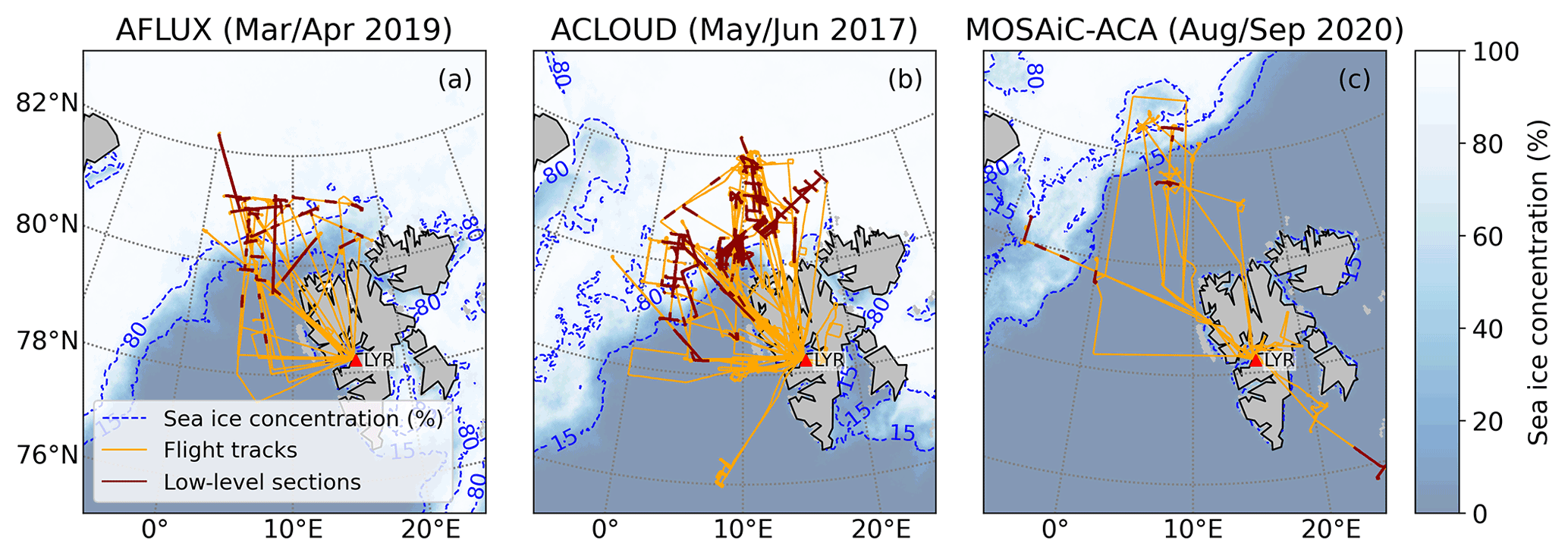
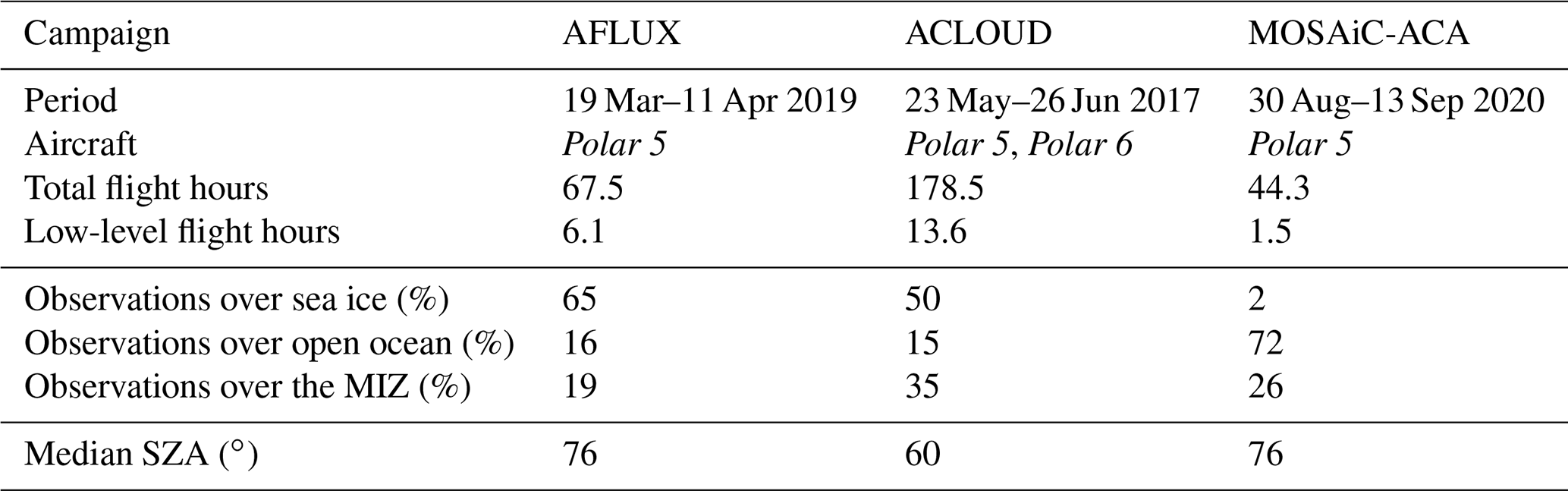
Figure 1 Flight tracks (orange) and low-level sections (dark red) performed during (a) AFLUX, (b) ACLOUD, and (c) MOSAiC-ACA based at Longyearbyen (LYR). Each panel shows the mean sea ice concentration f_ice (derived from space-borne observations, Spreen et al., 2008) present during the respective campaign, the dashed blue lines indicate the 15 % and 80 % isolines of f_ice that confine the MIZ according to the definition of Strong and Rigor (2013).

2 Observations

2.1 Airborne campaigns and instrumentation

To study atmospheric processes in the lower Arctic troposphere, three airborne campaigns were deployed to collect measurements of cloud, surface, and thermodynamic properties during different seasons near Svalbard. The Airborne measurements of radiative and turbulent FLUXes of energy and momentum in the Arctic boundary layer (AFLUX) campaign was conducted in early spring 2019 (Mech et al., 2022), while the Arctic CLoud Observations Using airborne measurements during polar Day (ACLOUD) campaign was performed in late spring/early summer 2017 (Wendisch et al., 2019). Additionally, the Multidisciplinary drifting Observatory for the Study of Arctic Climate – Airborne observations in the Central Arctic (MOSAiC-ACA) campaign was conducted in late summer 2020 and accompanied the MOSAiC drift expedition with airborne measurements (Shupe et al., 2022). Table 1 lists the periods during which the campaigns were deployed. During ACLOUD, the measurements were accomplished onboard the two research aircraft Polar 5 and Polar 6 from the Alfred Wegener Institute, Helmholtz Centre for Polar and Marine Research (Wesche et al., 2016). During the other campaigns, only Polar 5 was operated. The majority of the observations took place in the eastern Fram Strait north-west of Svalbard, the corresponding flight tracks are displayed in Fig. 1. Depending on the campaign, between 5 % and 20 % of the total flight time was dedicated to low-level flight sections, not exceeding a flight altitude of 250 m.

During the low-level sections, the broadband irradiances $F_{\text{sol}}^{\downarrow }$ and $F_{\text{sol}}^{\uparrow }$ on the one hand and $F_{\text{TIR}}^{\downarrow }$ and $F_{\text{TIR}}^{\uparrow }$ on the other hand were measured by pairs of upward- and downward-directed pyranometers (sensitive in the solar range between 0.2–3.6 µm) and pyrgeometers (sensitive in the TIR range between 4.5–42 µm) and recorded at a frequency of 20 Hz. An inertia correction was applied, which enables one to resolve fluctuations in the order of 2 s and to remove the inertia-induced time shift of the time series (Ehrlich and Wendisch, 2015). Furthermore, the impact of the aircraft attitude on $F_{\text{sol}}^{\downarrow }$ was accounted for by a common correction method (Bannehr and Schwiesow, 1993). Because of remaining uncertainties in the estimation of the fraction of direct solar irradiance, the irradiance data for aircraft attitude angles exceeding 5^∘ in roll and pitch angle were discarded. From the broadband irradiance measurements, F_net,sol,cld and F_net,TIR,cld (Eqs. 1 and 2) and the surface albedo (ratio of $F_{\text{sol}}^{\uparrow }$ and $F_{\text{sol}}^{\downarrow }$) in mostly cloudy conditions were derived. The exclusion of data due to the aircraft attitude and severe icing of the instruments, led to a reduction of the low-level data set by 41 %, 63 %, and 44 % for AFLUX, ACLOUD, and MOSAiC-ACA, respectively. The remaining low-level flight time used for the analysis is given in Table 1.

Although the measurements were not performed directly at the surface, the impact of the atmosphere below the aircraft is small if no cloud or fog layers are present there. For a flight altitude of 100 m, radiative transfer simulations for different cloud and albedo properties revealed an underestimation of less than 1.3 W m⁻² for CRE_sol and an overestimation of less than 1.25 W m⁻² for CRE_TIR compared to the surface. Larger differences are expected for the occasionally occurring sea smoke below the aircraft. However, the analysis focuses on the radiative effect of clouds above the flight altitude, i.e. neglecting the sea smoke. Only in the case of indirect effects (e.g. change of the measured albedo by the sea smoke) is its influence discussed in the remainder of this study.

Additionally, the sea ice concentration f_ice was derived from measurements of a three-channel digital camera equipped with a 180^∘ fisheye lens (sampling frequency: one image every 6 s). The individual pixels of the radiance-calibrated images of the fisheye camera were classified into the different surface types based on their reflection characteristics (Becker et al., 2022), in order to derive the cosine-weighted surface type fraction of each image. Based on the transmissivity of the clouds, which is the fraction of the downward irradiances measured in mostly cloudy atmospheric conditions and simulated for cloud-free conditions, an equivalent LWP was retrieved using the method of Stapf et al. (2020) and assuming clouds with a droplet r_eff of 8 µm. Despite the neglected cloud ice and the fixed r_eff in the retrieval, the equivalent LWP provides a robust estimate of the optical thickness of the clouds. Regular profiles of temperature and relative humidity were obtained using the in situ meteorological measurements during aircraft ascents and descents, sondes dropped from the aircraft, and, for the higher atmosphere, radiosoundings launched at Ny-Ålesund. Measurements of profiles of the cloud liquid water content (LWC) obtained from various in situ cloud probes were used to retrieve cloud boundaries. Further details on the aircraft instrumentation and data processing are provided by Ehrlich et al. (2019b) and Mech et al. (2022).

2.2 Sea ice situation during the campaigns

The different distributions of sea ice in the Fram Strait region during the three campaigns investigated in this paper are depicted in Fig. 1 based on the space-borne observations of f_ice (Spreen et al., 2008). While the sea ice edge was roughly located between 80–81^∘ N during AFLUX (Fig. 1a), it was situated slightly further south during ACLOUD (Fig. 1b). During both campaigns, the region east of Svalbard was covered by almost closed sea ice. Since MOSAiC-ACA was performed temporally close to the annual sea ice minimum, ice-free conditions were present east of the island, and the sea ice edge in the Fram Strait was mostly north of 82^∘ N. It was reached by Polar 5 only for a short flight section (Fig. 1c). Consequently, more than half of the low-level observations during AFLUX and ACLOUD were performed over closed sea ice, while during MOSAiC-ACA, the fraction of observations over sea ice amounts to only 2 % and strongly limits the statistical representation of this situation. Instead, almost three quarters of the low-level observations were performed over open ocean during MOSAiC-ACA compared to about 15 % during the other campaigns (Table 1). Note that for the low-level observations, the marginal sea ice zone (MIZ) comprises all observations with f_ice between 0.05 and 0.95 and, thus, deviates from the MIZ definition of Strong and Rigor (2013), where f_ice is between 0.15 and 0.8. These modified thresholds are motivated by the strong impact of the surface type on the surface radiative properties, which significantly changes for small fractions of sea ice or open ocean already and requires a more rigorous separation of the MIZ (e.g. Becker et al., 2022).

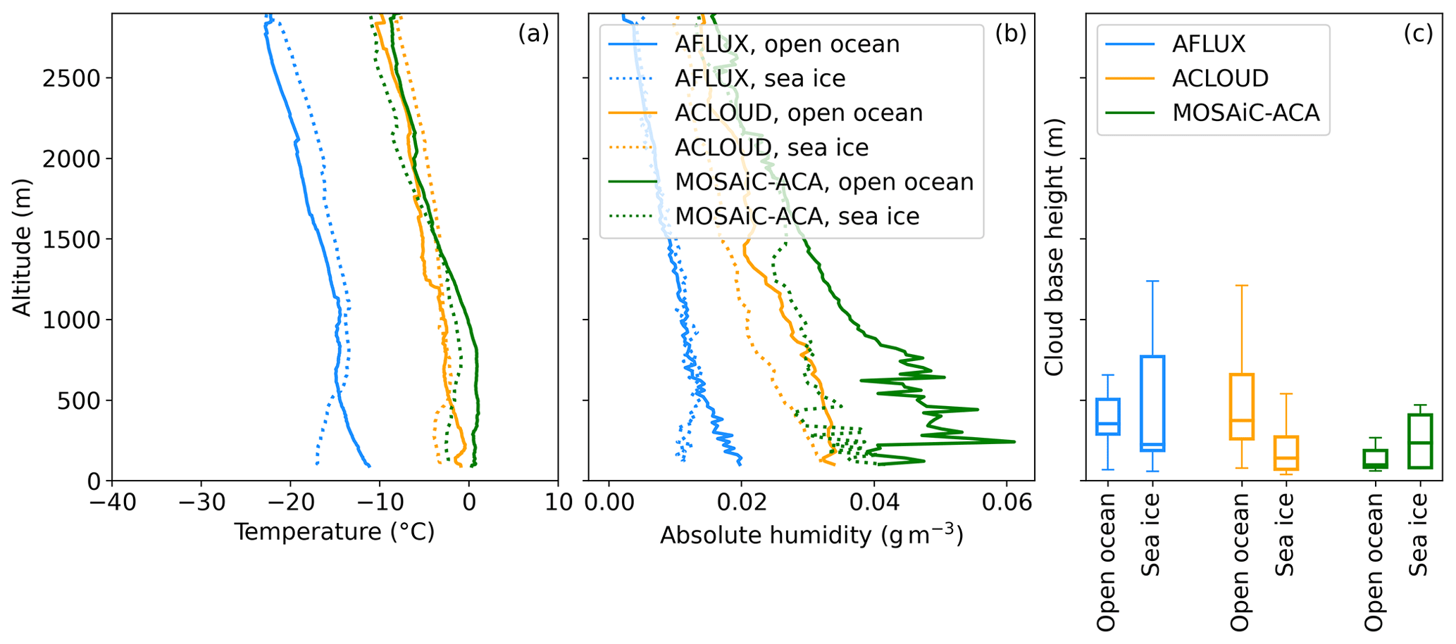
Figure 2 Mean profiles of (a) temperature and (b) absolute humidity obtained during aircraft ascents and descents of the individual campaigns (colour-coded), separated for the different surface types (linestyle-coded). (c) Box-whisker plots of the cloud base height obtained from the in situ cloud probes (see text for details). The surface type separation is based on the space-borne observations of f_ice (Spreen et al., 2008) and the surface type definition of Strong and Rigor (2013).

2.3 Thermodynamic profiles and cloud base height

Mean profiles of various thermodynamic properties measured during the campaigns are shown in Fig. 2a and b. According to the time of the year, AFLUX showed significantly colder temperatures compared to the remaining campaigns (Fig. 2a). While the mean near-surface temperature over sea ice was −16 ^∘C during AFLUX, it was around −3 ^∘C during ACLOUD and MOSAiC-ACA. The near-surface temperature over open ocean was close to the freezing point during ACLOUD and MOSAiC-ACA and below −10 ^∘C during AFLUX. Over sea ice, a surface-based temperature inversion was present during all campaigns but strongest during AFLUX. In contrast, temperature inversions were weak or absent over open ocean, with the least stable mean profile obtained for AFLUX. In higher altitudes, the mean profiles over sea ice and open ocean of the same campaign agreed well.

The emission and absorption by the atmospheric water vapour, relevant for the surface F_net,TIR, depends on the absolute humidity (AH), which is shown in Fig. 2b. Due to the lower equilibrium pressure and the resulting lower concentration of water vapour for colder temperatures, AFLUX showed the lowest AH. The differently shaped temperature profiles over sea ice and open ocean below 500 m are imprinted in the mean AH profile. Despite the comparable temperature range, the AH was significantly lower during ACLOUD than during MOSAiC-ACA, which is due to the lower relative humidity (RH, not shown). Furthermore, the lower RH over sea ice reduced the AH compared to open ocean during ACLOUD. During MOSAiC-ACA, both the higher temperature and the larger RH caused the increased AH over open ocean below 1500 m.

The surface CRE_TIR largely depends on the cloud base temperature, which is determined by the location of the cloud within the temperature profile. Figure 2c shows statistics of the cloud base height obtained from the in situ cloud probes. Clouds were identified by a LWC threshold of 0.005 g cm⁻³. During AFLUX, the median cloud base height over open ocean was 352 m. Over sea ice, the median cloud base height was lower (223 m) but more variable. The typical cloud base temperature range is estimated from the mean temperature (Fig. 2a) in the altitudes corresponding to the interquartile range (IQR) of the cloud base height. For AFLUX, the cloud base temperature was in the range of −14 ^∘C over sea ice and between −13 and −17 ^∘C over open ocean. During ACLOUD, the median cloud base height of 372 m over open ocean was similar compared to AFLUX, while clouds over sea ice were significantly lower (140 m). The resulting cloud base temperatures range between −3 and 0 ^∘C over open ocean and around −3 ^∘C over sea ice. During MOSAiC-ACA, the median cloud base height over sea ice was 234 m, while clouds over open ocean showed very low bases (97 m). The cloud base temperatures were about 0 and −2 ^∘C over open ocean and sea ice, respectively. In general, the slightly colder cloud base temperatures over sea ice seem to result from the colder low-level temperatures rather than from the different cloud base heights.

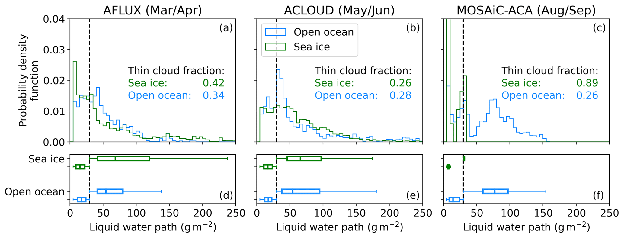
Figure 3 Probability density function of the equivalent LWP over sea ice and open ocean (colour-coded) for (a) AFLUX, (b) ACLOUD, and (c) MOSAiC-ACA. Only observations classified as cloudy (equivalent LWP > 5 g m⁻²) were considered. The vertical dashed lines located at 30 g m⁻² indicate the threshold used for the separation of thin and thick clouds. The numbers in panels (a–c) represent the fraction of observations with thin clouds with respect to the total amount of cloudy observations. (d–f) Box-whisker plots of the equivalent LWP separating thin (left boxplots) and thick clouds (right boxplots).

2.4 Cloud liquid water path

The statistical characteristics of the equivalent cloud LWP assembled during the campaigns are illustrated in Fig. 3 as a rough measure for optical thickness. During AFLUX (Fig. 3a), clouds with an equivalent LWP below 10 g m⁻² were most frequent over sea ice, while the largest mode of equivalent LWP over open ocean occurs between 30 and 50 g m⁻². CRE_TIR is especially sensitive to the LWP of optically thin clouds below 30 g m⁻² (e.g. Shupe and Intrieri, 2004; Ebell et al., 2020) but almost constant for larger LWPs. Accordingly, this threshold was used to distinguish between thin and thick clouds, which are analysed separately. Corresponding to the probability density functions (PDFs), the median equivalent LWP of thin clouds is lower over sea ice than over open ocean, with values of 15 and 18 g m⁻², respectively (Fig. 3d). In contrast, the median of thick clouds is larger over sea ice. However, thin clouds occurred more frequently over sea ice compared to open ocean (numbers in Fig. 3a).

The PDF of the equivalent LWP derived from ACLOUD measurements (Fig. 3b) reveals a similar distribution of thin clouds over sea ice and open ocean. Both surface types showed similar median values for thin clouds (around 17 g m⁻², Fig. 3e). Over open ocean, clouds with an equivalent LWP of 30–50 g m⁻² were most common, while larger LWPs were more frequent over sea ice than over open ocean. Thus, the median equivalent LWP of thick clouds was larger over sea ice. The thin cloud fraction was slightly lower over sea ice compared to open ocean. Compared to AFLUX, thin clouds occurred significantly less frequently over both surface types.

During MOSAiC-ACA (Fig. 3c), the vast majority of the clouds over the sparsely sampled sea ice showed an extremely low equivalent LWP. The median equivalent LWP of thin clouds was 7 g m⁻² (Fig. 3f), and almost 90 % of the sampled clouds were thin. These observations are statistically not representative and very likely do not reflect typical conditions present over sea ice during this season. In contrast, the equivalent LWP of clouds over open ocean showed a broader distribution with a strong mode of thick clouds. The thin cloud fraction over open ocean was similar to the one observed during ACLOUD. Compared to the other campaigns, the median of the equivalent LWP of thin clouds over open ocean was slightly lower and amounted to 14 g m⁻².

3 Simulation of the net irradiance in assumed cloud-free conditions

3.1 Radiative transfer simulations

Section 2.1 describes the measurements of F_net,sol,cld (in mostly cloudy conditions) and F_net,TIR,cld. To calculate both CRE_sol and CRE_TIR, F_net,sol,cf and F_net,TIR,cf need to be simulated. For this purpose, the one-dimensional radiative transfer solver DISORT (DIScrete Ordinate Radiative Transfer) is applied (Stamnes et al., 1988), which is embedded in the library for radiative transfer libRadtran (Emde et al., 2016). The radiative transfer simulations were performed using the method proposed by Stapf et al. (2020). For both spectral ranges, the atmospheric state was obtained from thermodynamic profiles measured during ascents or descents adjacent to the respective low-level section, which were topped by the temporally closest radiosounding. Aerosol properties were not considered in the simulations. In addition to these settings, F_net,TIR,cf was simulated using a surface emissivity of 0.99 for snow (Warren, 1982), which is similar for open ocean at least for the atmospheric window (8–13 µm) region (Konda et al., 1994). Instead of the surface emissivity, the simulation of F_net,sol,cf additionally requires the SZA and the definition of the local surface albedo in cloud-free conditions, which is different from the surface albedo measured in cloudy conditions. From the simulations, the direct/diffuse fraction of $F_{\text{sol}}^{\downarrow }$ was obtained for cloud-free conditions.

3.2 Impact of clouds on the surface albedo

3.2.1 Surface albedo over open ocean in cloud-free and cloudy conditions

While Stapf et al. (2020) analysed the impact of clouds on the surface albedo of sea ice, the following analysis focuses on similar effects influencing the surface albedo of open ocean. The change of the broadband albedo due to the presence of clouds is a result of two effects: first, the changing amount of direct and diffuse solar radiation (geometry effect) and, second, the changing spectral distribution of the downward solar irradiance (spectral weighting effect). In general, the broadband surface albedo α is given by

$$\begin{array}{}\text{(5)}& \mathit{\alpha }={\displaystyle \frac{F_{\text{sol}}^{\uparrow }}{F_{\text{sol}}^{\downarrow }}}={\displaystyle \frac{{\int }_{\text{sol}}{F}_{\mathit{\lambda }}^{\uparrow }\left(\mathit{\lambda }\right)\mathrm{d}\mathit{\lambda }}{{\int }_{\text{sol}}{F}_{\mathit{\lambda }}^{\downarrow }\left(\mathit{\lambda }\right)\mathrm{d}\mathit{\lambda }}}.\end{array}$$

$F_{\text{sol}}^{\uparrow }$ and $F_{\text{sol}}^{\downarrow }$ are obtained by integrating the spectral upward and downward irradiances, $F_{\mathit{\lambda }}^{\uparrow }$ and $F_{\mathit{\lambda }}^{\downarrow }$, over the wavelengths λ of the solar range (indicated by ∫_sol). To introduce the spectral albedo α_λ, $F_{\mathit{\lambda }}^{\uparrow }$ is replaced by $F_{\mathit{\lambda }}^{\downarrow }$ and α_λ:

$$\begin{array}{}\text{(6)}& \mathit{\alpha }=\underset{\text{sol}}{\int }{\mathit{\alpha }}_{\mathit{\lambda }}\left(\mathit{\lambda }\right)\cdot {\displaystyle \frac{F_{\mathit{\lambda }}^{\downarrow }\left(\mathit{\lambda }\right)}{{\int }_{\text{sol}}{F}_{\mathit{\lambda }}^{\downarrow }\left(\mathit{\lambda }\right)\mathrm{d}\mathit{\lambda }}}\mathrm{d}\mathit{\lambda }.\end{array}$$

Equation (6) shows that the broadband albedo represents a weighted average depending on α_λ and $F_{\mathit{\lambda }}^{\downarrow }$, which serves as a weight function. While α_λ changes due to the geometry effect, a change of the normalized weight function w, with

$$\begin{array}{}\text{(7)}& w={\displaystyle \frac{F_{\mathit{\lambda }}^{\downarrow }\left(\mathit{\lambda }\right)}{{\int }_{\text{sol}}{F}_{\mathit{\lambda }}^{\downarrow }\left(\mathit{\lambda }\right)\mathrm{d}\mathit{\lambda }}},\end{array}$$

describes the spectral weighting effect. Both effects are analysed in the following.

Over open ocean, α_λ and w were simulated with libRadtran, applying a parameterization of the directional reflection of open-ocean surfaces with varying SZA and wind speed in 10 m altitude (Cox and Munk, 1954). To illustrate the effect of clouds on the surface albedo, simulations containing boundary layer clouds (400–600 m) with variable LWP and a fixed r_eff of 8 µm were performed.

The change of α_λ due to different illumination geometries is shown in Fig. 4a. In cloud-free conditions, α_λ is dominated by the reflection of the direct component of $F_{\mathit{\lambda }}^{\downarrow }$. Beside their different patterns, α_λ is significantly larger for a SZA of 75^∘, which is representative for AFLUX and MOSAiC-ACA, compared to a SZA of 60^∘, representative for ACLOUD. The almost constant α_λ above 1000 nm is 0.20 for 75^∘ but only 0.07 for 60^∘. This difference is due to the enhanced specular reflection at the air–water interface for larger incident angles (i.e. SZA), according to Fresnel's equations. In cloudy conditions (LWP of 80 g m⁻²), α_λ is modified by the predominating diffuse illumination and reveals slightly lower values compared to the cloud-free case with a SZA of 60^∘. The best agreement between α_λ in cloudy and cloud-free conditions was found for a SZA of 52^∘ (not shown), which can be referred to as an effective incident zenith angle in cloudy conditions. Thus, the geometry effect causes a lower surface albedo in cloudy conditions compared to cloud-free conditions for SZAs typical for the Arctic, with a larger difference for larger SZAs. Due to a reduction of specular reflection on a roughened surface, this difference decreases as the wind speed is increased, especially for large SZAs (Jin et al., 2004).

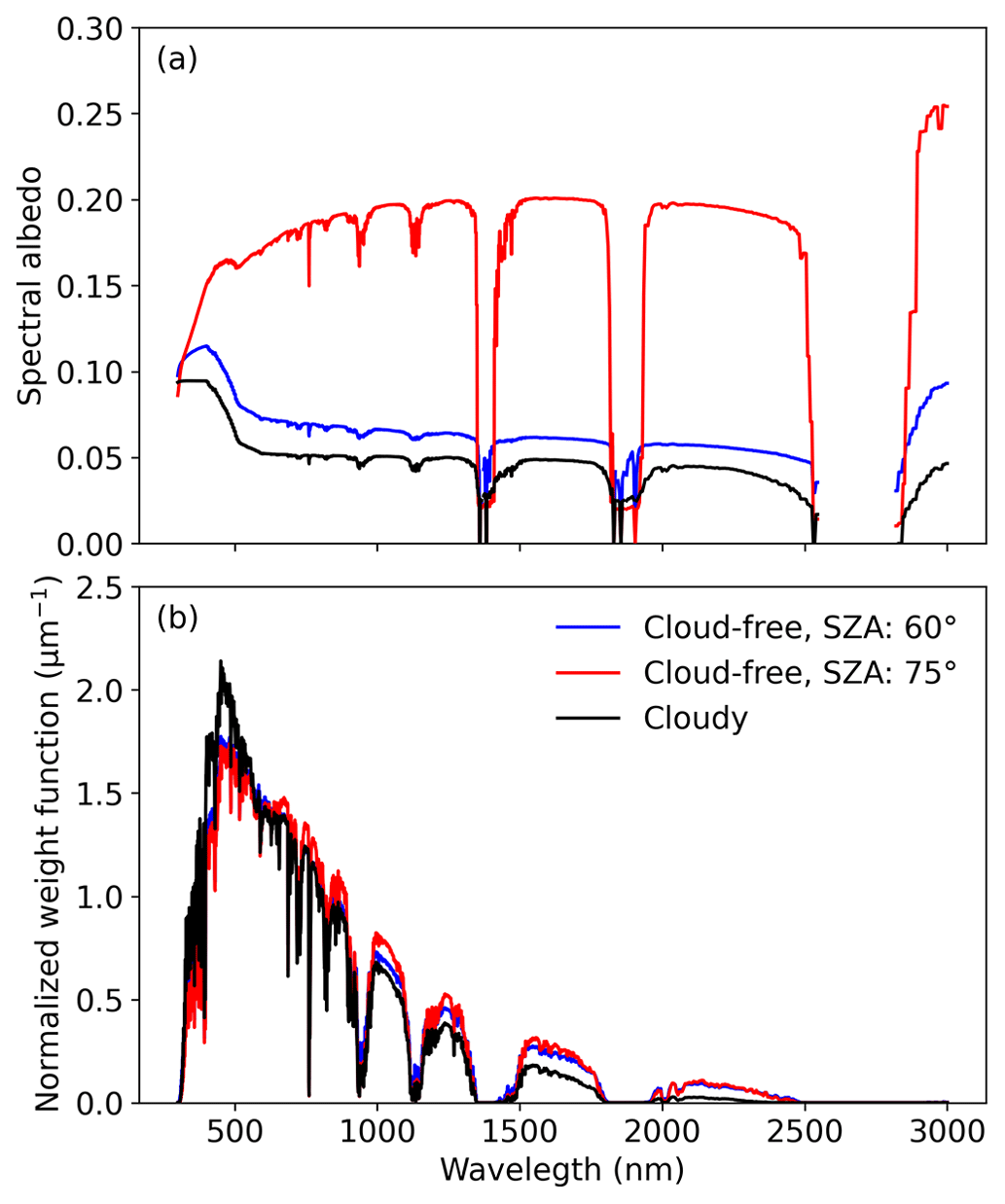
Figure 4 (a) Simulations of the spectral surface albedo α_λ of open ocean for two different SZAs in cloud-free conditions and for cloudy conditions (LWP of 80 g m⁻², independent of SZA). (b) Simulations of the spectral normalized weight functions w for the same scenarios. The wind speed of 1 m s⁻¹ represents a calm surface.

The broadband albedo is also affected by the spectral distribution of the incident irradiance (Eq. 6), which is described by w and can be modified by clouds. Spectra of w corresponding to the cases discussed above are illustrated in Fig. 4b. At visible wavelengths (e.g. 500 nm), w is larger in cloudy conditions compared to cloud-free conditions, while the situation is reversed in the near-infrared (NIR) range (e.g. 1600 nm) due to enhanced absorption by cloud particles. Consequently, α_λ in the visible wavelength range, which is slightly higher compared to α_λ in the NIR range, contributes more strongly to the broadband albedo in cloudy conditions than it does in the cloud-free case. This spectral weighting partly counteracts the spectral albedo geometry effect on the broadband albedo.

3.2.2 Parameterization of the open-ocean and sea ice albedo in cloud-free conditions

To account for the cloud-induced change of the surface albedo in the calculation of the cloud-free net irradiance, parameterizations are used to retrieve the surface albedo in cloud-free conditions. The sea ice albedo is retrieved using the method described by Stapf et al. (2020), which is based on the parameterization of Gardner and Sharp (2010). This parameterization depends on the SZA, the equivalent cloud LWP, and the specific surface area (SSA) of snow, which is a measure for the snow grain size and was retrieved from the measured surface albedo. For open ocean, the parameterization of Jin et al. (2011) was used to obtain the surface albedo in cloud-free conditions. The required input includes the SZA, the wind speed measured in flight altitude and scaled down to 10 m using the logarithmic wind profile with a roughness length of 2 × 10⁻⁴ m (offshore conditions), and the simulated fraction of diffuse incident radiation in cloud-free conditions (Sect. 3.1). For a mixture of open ocean and sea ice, the parameterized albedos of both surface types are linearly combined using f_ice obtained from the fisheye camera (Becker et al., 2022).

Figure 5 illustrates the parameterized broadband albedo as a function of the LWP. The broadband open-ocean albedo (Fig. 5a) decreases with increasing LWP, which indicates that the geometry effect dominates over the spectral weighting effect. This is due to the relatively low spectral differences of the open ocean α_λ (Fig. 4a). Similar to α_λ, the broadband open-ocean albedo in diffuse conditions (LWPs larger than 20 g m⁻²) is independent of the SZA and converges at 0.06, while the albedo in cloud-free conditions increases for increasing SZA. Thus, the cloud-free albedo is only slightly larger than the diffuse albedo for a SZA of 60^∘ but reaches 0.16 for a SZA of 75^∘. For larger wind speeds, the difference between the cloudy and cloud-free albedos decreases (not shown).

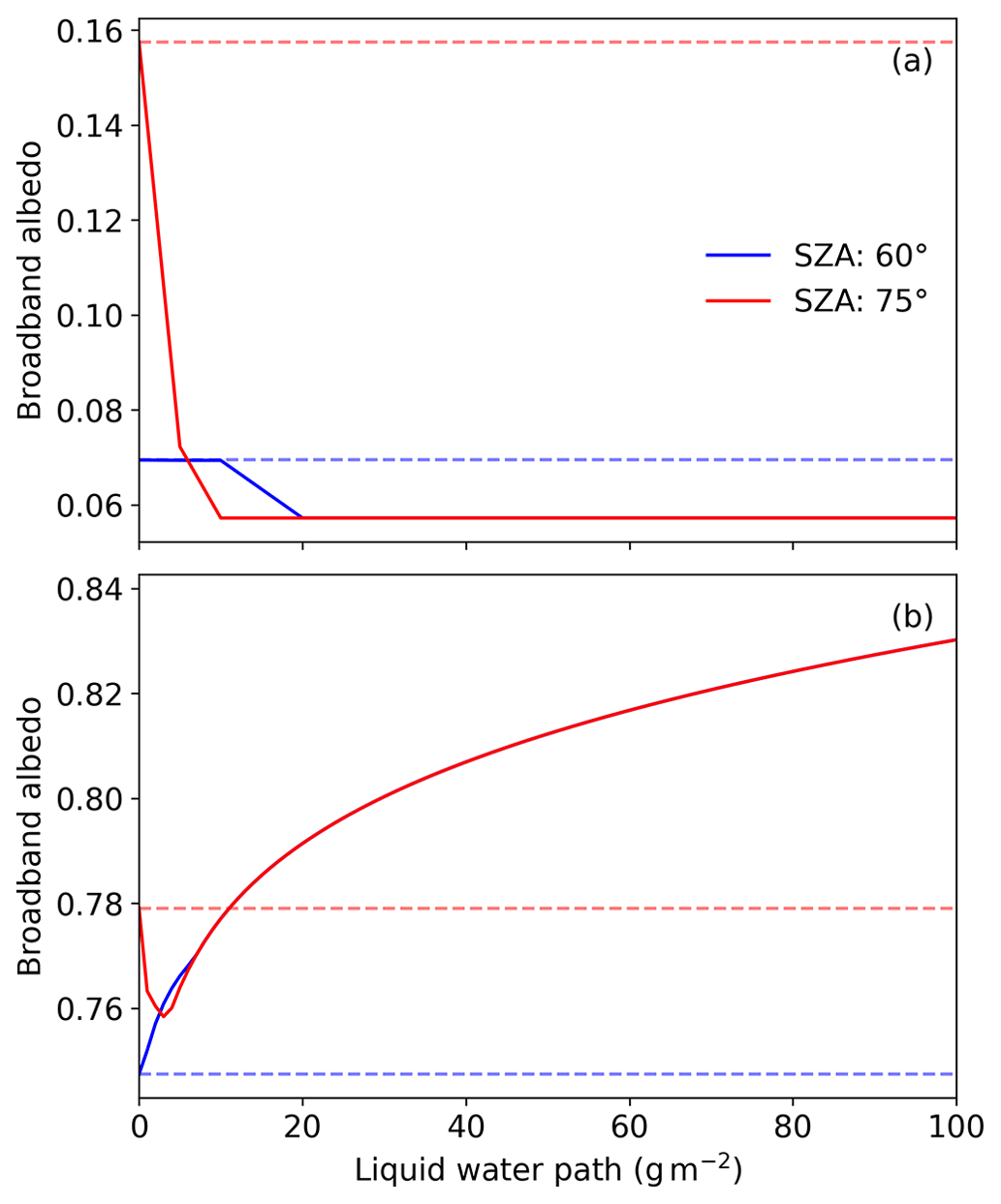
Figure 5 Broadband albedo of (a) open ocean and (b) sea ice as a function of the cloud LWP for different SZAs. The open-ocean albedo is based on the parameterization of Jin et al. (2011), with a 10 m wind speed of 1 m s⁻¹. The sea ice albedo is based on the parameterization of Gardner and Sharp (2010), with a SSA of 80 m² kg⁻¹. The attenuated dashed lines represent the respective cloud-free surface albedos.

In contrast to open ocean, α_λ of snow-covered sea ice shows large discrepancies, with high values in the visible and low values in the NIR range (e.g. Stapf et al., 2020, their Fig. 3). Thus, the spectral weighting effect becomes more dominant and leads to an increase of the broadband albedo with increasing LWP (Fig. 5b). While this is true for the entire LWP range for a SZA of 60^∘, a slight albedo decrease is observed for the lowest LWPs and a SZA of 75^∘. This feature arises from the geometry effect surpassing the spectral weighting effect for optically thin clouds when the Sun is low enough. The cloud-free albedo is 0.75 and 0.78 for SZAs of 60 and 75^∘, respectively. Similar to open ocean, the surface albedo of sea ice does not differ with SZA in diffuse conditions. Consequently, the albedo differences between cloudy and cloud-free conditions are larger for lower SZAs within the typical LWP range.

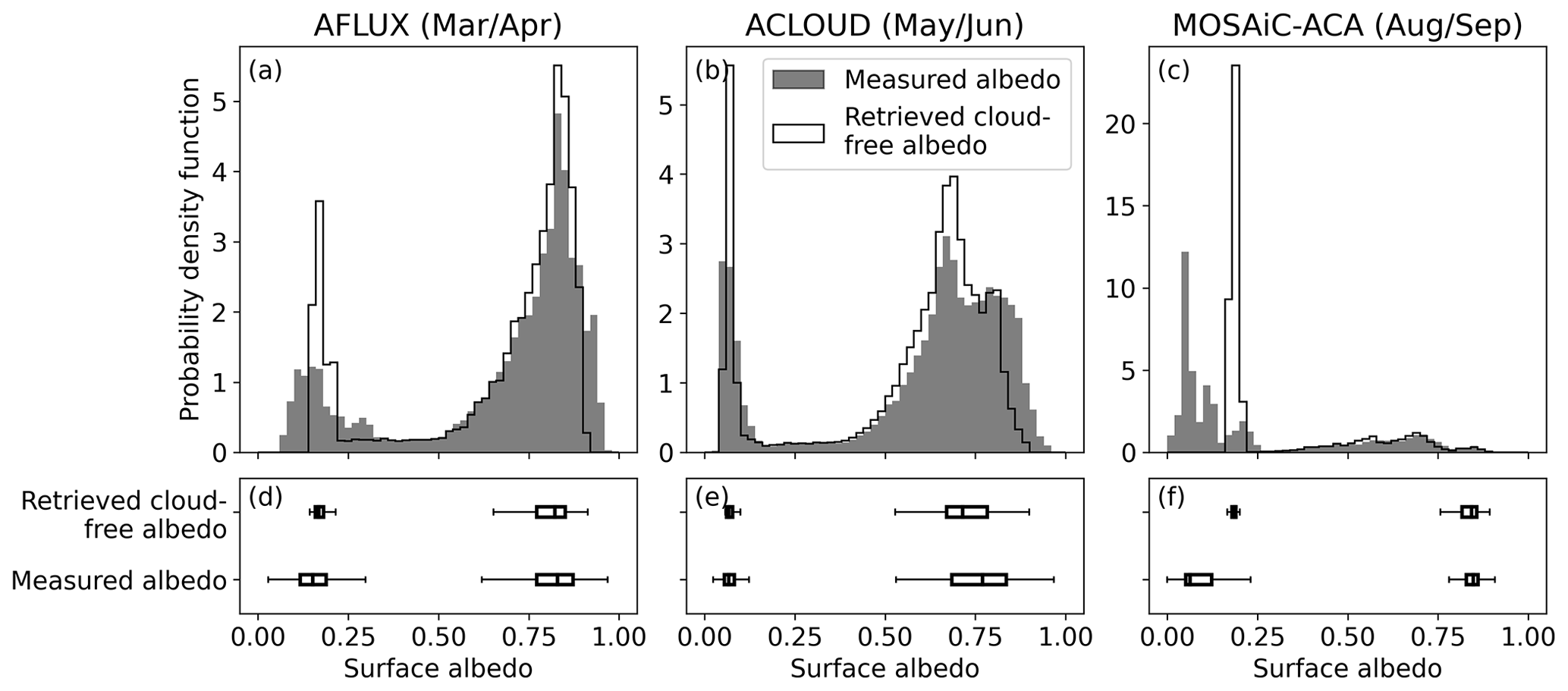
Figure 6 Probability density function of the surface albedos measured in mostly cloudy conditions (shadings) and retrieved for cloud-free conditions (lines) for (a) AFLUX, (b) ACLOUD, and (c) MOSAiC-ACA. (d–f) Box-whisker plots of the retrieved cloud-free and measured surface albedo separated for open ocean (left boxplots) and sea ice (right boxplots).

To retrieve the cloud-free surface albedo from the mostly cloudy albedo measurements performed during the low-level sections, the surface albedo parameterizations were applied to the measurements of the three campaigns. Figure 6 illustrates the effect of the cloud-induced albedo change by comparing the frequency distributions of the measured (mostly cloudy) and retrieved (cloud-free) surface albedos. The left and the right mode of all distributions correspond to the open-ocean and sea ice surfaces, respectively. Compared to the measured albedo, the distribution of the retrieved cloud-free albedo is narrowed over open ocean during AFLUX (Fig. 6a and d). Although a notably higher open-ocean albedo would be expected in cloud-free conditions for SZAs present during AFLUX (Fig. 5a), the measured and retrieved median albedo values of 0.15 and 0.17, respectively, did not differ significantly. This is probably due to the frequently occurring sea smoke between the aircraft and the ocean surface, which artificially increased the measured albedo compared to the expected values (Fig. 5a). For the snow-covered sea ice, the median values of 0.83 and 0.82 indicate only small differences between the measured albedo and the retrieved cloud-free albedo, which is in accordance with Fig. 5b for the typical SZA range during AFLUX. Similarly, no significant difference between measured and retrieved cloud-free albedo of open ocean could be observed during ACLOUD (Fig. 6b and e). However, as suggested by Fig. 5b, a significant albedo shift over sea ice is obvious for ACLOUD, where the median of the surface albedo decreased from 0.77 in the observed cloudy conditions to 0.71 for the retrieved cloud-free albedo. In general, the observations during ACLOUD are characterized by a lower sea ice albedo compared to AFLUX, which is due to the onset of the melting season. Despite the similar SZA range, the cloud-induced change of the open-ocean albedo showed different effects for AFLUX and MOSAiC-ACA. The median of the measured albedo was only 0.06 during the latter (Fig. 6c and f). However, the median retrieved cloud-free albedo of 0.19 was similar to the value retrieved for AFLUX. The rarely sampled sea ice during MOSAiC-ACA is only expressed by the rightmost, very small mode. Similar to AFLUX, the sea ice albedo did not change significantly between cloudy and cloud-free conditions. The mode located roughly between 0.25 and 0.75 represents observations over the MIZ.

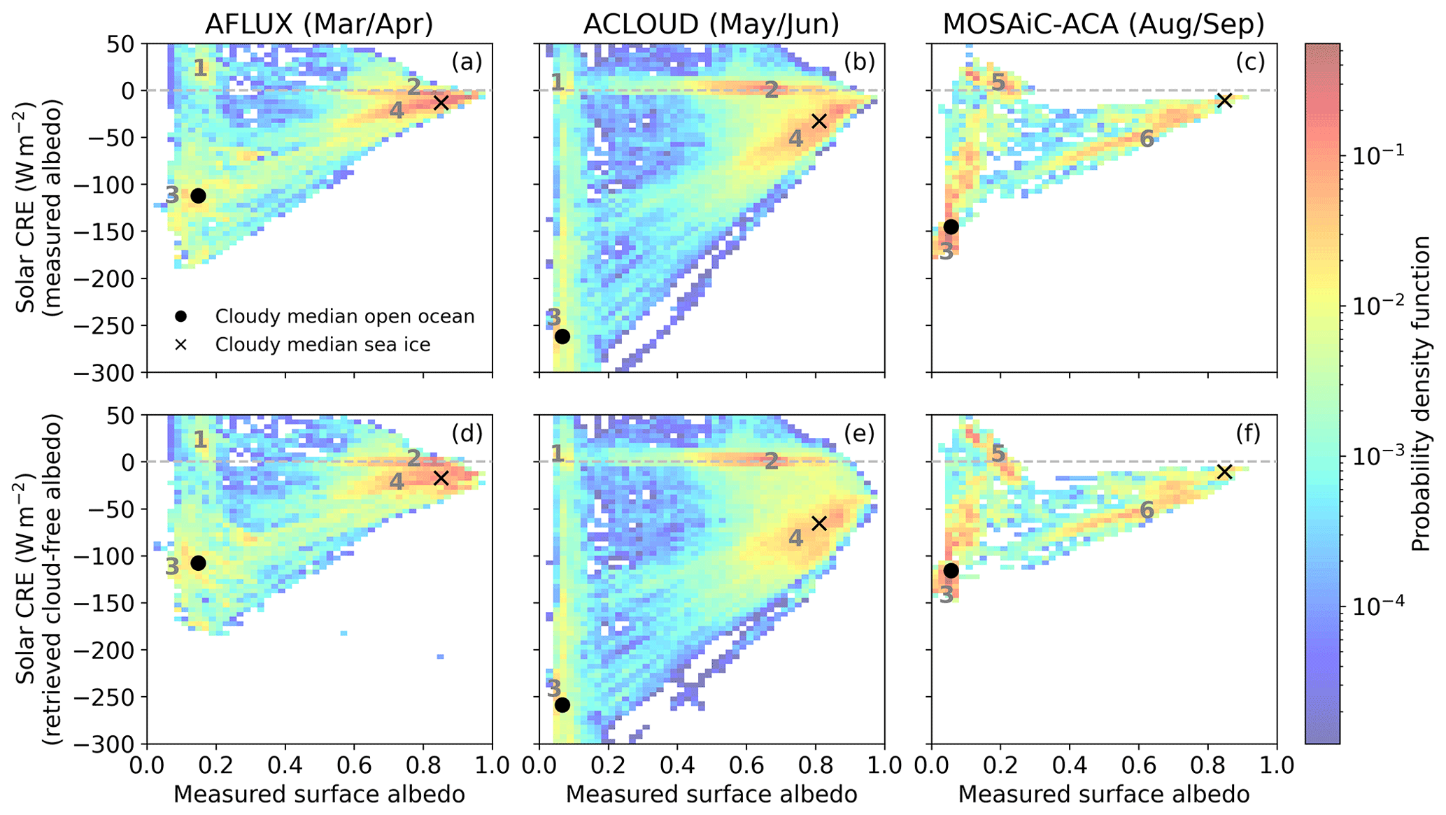
Figure 7 Two-dimensional probability density function of CRE_sol and the measured (mostly cloudy) surface albedo (as an indicator for the surface type) for AFLUX (a, d), ACLOUD (b, e), and MOSAiC-ACA (c, f). The upper row (a–c) shows the distributions of CRE_sol neglecting the cloud-induced change of the surface albedo, while this effect is included in the lower row (d–f). The horizontal dashed lines mark a CRE_sol of 0 W m⁻². The symbols represent the median of CRE_sol and the measured surface albedo over the surface types given in the legend in panel (a) and only considering cloudy observations (equivalent LWP > 5 g m⁻²). The numbered modes represent (1) cloud-free open ocean, (2) cloud-free sea ice, (3) cloudy open ocean, (4) cloudy sea ice, (5) thin/broken clouds, and (6) cloudy MIZ conditions.

4 Cloud radiative effect

4.1 Solar cloud radiative effect

The variability of CRE_sol at the surface during the three campaigns is assessed by analysing the frequency distributions of CRE_sol as a function of the strongly influential measured surface albedo, which are shown in Fig. 7. To quantify the impact of the cloud-induced albedo change on CRE_sol, two distributions are presented for each campaign. While the cloud-induced surface albedo change is neglected in Fig. 7a–c, Fig. 7d–f shows CRE_sol corrected for this effect. For AFLUX and ACLOUD, the distributions of Fig. 7 reveal four distinct modes (indicated by the numbers 1–4). The modes 1 and 2 are located around or slightly above 0 W m⁻² and reflect mainly cloud-free conditions, while the remaining modes (modes 3 and 4) indicate the cooling effect of clouds in the solar range. Through their distinct surface albedos, CRE_sol over open-ocean (mode 3) and sea ice (mode 4) surfaces are clearly distinct. During MOSAiC-ACA (Fig. 7c and f), thin or broken clouds (mode 5) and frequent observations over the MIZ in cloudy conditions (mode 6) altered the mode structure.

The comparison of the two distributions per campaign exposes the shift of several modes due to the cloud-induced albedo change. For AFLUX (Fig. 7a and d), only minor changes can be observed, which is in accordance with the similar distributions of measured and retrieved (cloud-free) surface albedo (Fig. 6a). The albedo change increased (reduced) the median CRE_sol over open ocean (sea ice) by 4 W m⁻². The artificial absence of a larger CRE_sol increase over open ocean is due to the sea smoke and the resulting too high measured surface albedo discussed in Sect. 3.2.2. The actual change of CRE_sol remains unclear. As discussed by Stapf et al. (2020), the increased albedo of sea ice in cloudy conditions caused a significant shift of mode 4 during ACLOUD (Fig. 7b and e) and almost doubled the median of the uncorrected CRE_sol of −33 W m⁻². In contrast, CRE_sol over open ocean was hardly affected. During MOSAiC-ACA, the weakening of the solar cooling effect due to the increased open-ocean albedo in cloud-free conditions (Fig. 6c) is expressed by the shift of mode 3 (Fig. 7c and f). The median of the uncorrected CRE_sol (−145 W m⁻²) imposed an artefact of 29 W m⁻² cooling due to the neglect of the cloud-induced albedo change. The sea-ice-dominated MIZ (mode 6) is not affected by the albedo change because the negligible increase of the sea ice albedo and the more significant decrease of the open-ocean albedo towards cloud-free conditions cancel one another.

Using CRE_sol, accounting for the cloud-induced albedo change (Fig. 7d–f), the features of the individual distributions and the differences among them are discussed in the following. For AFLUX (Fig. 7d), mode 1 over open ocean shows a remarkably positive CRE_sol with a median of 20 W m⁻² for an equivalent LWP of less than 5 g m⁻². This solar warming effect is due to broken cumulus clouds, which often enhance $F_{\text{sol}}^{\downarrow }$ compared to a cloud-free situation for several minutes by scattering additional solar radiation towards the surface (cloud enhancement; Mol et al., 2023). Broken clouds frequently occur during cold air outbreaks over open ocean, when the cold air advected over the warm ocean reduces the thermodynamic stability and leads to the formation of cloud streets (e.g. Brümmer, 1996). Thus, mode 1 combines cloud-free situations with broken cloud observations, the latter producing a low retrieved equivalent LWP that is indistinguishable from cloud-free conditions. Due to the high surface albedo of sea ice (larger than 0.6), the magnitude of CRE_sol was small over this surface type (mode 4, median of −17 W m⁻², black cross in Fig. 7d) and could hardly be distinguished from the absent CRE_sol in cloud-free conditions (mode 2), especially for very bright scenes. In contrast, the low open-ocean albedo enabled a much stronger solar cooling effect of the clouds (mode 3), with a median CRE_sol of −108 W m⁻² (black dot in Fig. 7d).

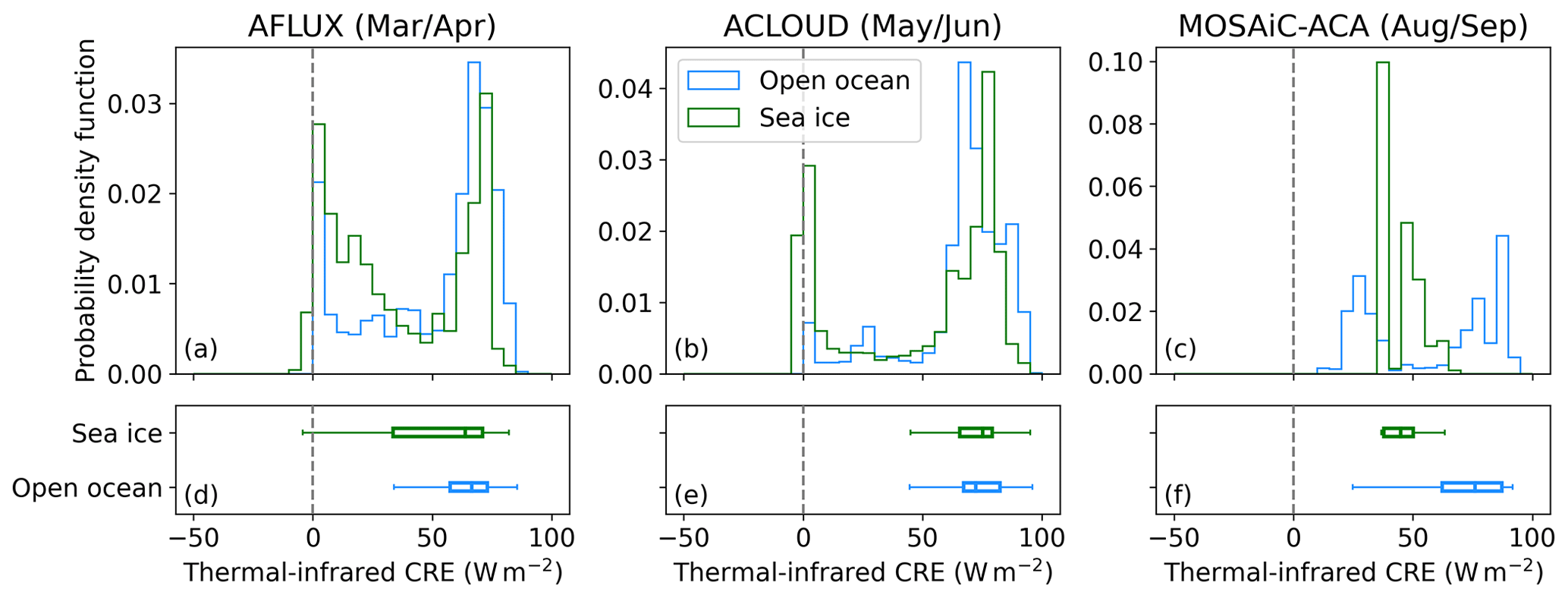
Figure 8 Probability density function of CRE_TIR for (a) AFLUX, (b) ACLOUD, and (c) MOSAiC-ACA, separated for sea ice and open ocean (colour-coded). (d–f) Box-whisker plots of CRE_TIR only considering cloudy observations (equivalent LWP > 5 g m⁻²). The vertical dashed lines mark a CRE_TIR of 0 W m⁻². Note that, due to a lack of the corresponding observations, none of the modes in panel (c) represents actual cloud-free conditions. The thinnest clouds, however, revealed an equivalent LWP < 5 g m⁻² and thus did not contribute to the statistics shown in panel (f).

The CRE_sol distribution of ACLOUD (Fig. 7e) is shaped more clearly compared to AFLUX due to the better statistics of the data. CRE_sol over open ocean and sea ice (modes 3 and 4) reveals median values of −259 and −65 W m⁻², respectively, which indicates a significantly stronger solar cooling effect compared to AFLUX. Although the lower surface albedo contributed to this stronger cooling effect during ACLOUD, a normalization of CRE_sol with the cosine of the SZA (not shown) reveals that the major contribution to the CRE_sol differences between the two campaigns resulted from the different solar illumination as a consequence of the clearly distinct SZA ranges (Table 1). Note that the SZA exhibits not only an annual but also a daily cycle. However, since most of the flights were conducted around solar noon, the SZA variability within one campaign was small.

The observations from MOSAiC-ACA reveal a large variability and a relatively unclear mode structure (Fig. 7f), which is due to the much less significant statistics compared to the other campaigns (see Table 1). Modes 1 and 2 are missing in the distribution, since cloud-free conditions were not sampled during MOSAiC-ACA. Instead of mode 1, mode 5 represents broken or very thin clouds over open ocean. Similar to AFLUX, this mode peaks at positive CRE_sol values due to the broken cloud effect. However, in contrast to AFLUX, negative CRE_sol values were also observed, probably resulting from rather overcast thin cloud conditions. Due to the similar Sun elevation (Table 1), the median of CRE_sol over open ocean (−116 W m⁻², mode 3) was similar compared to AFLUX. In contrast to the other campaigns, the rare observations over homogeneous sea ice during MOSAiC-ACA are not reflected in an own mode. These observations are rather included in the cloudy MIZ mode (mode 6), which expands to albedo values of down to 0.4.

The present analysis indicates a significant variability of CRE_sol between the campaigns and the underlying surface types. In accordance with previous studies (e.g. Intrieri et al., 2002; Miller et al., 2015), CRE_sol between the campaigns mostly varied due to the seasonally changing SZA, with a stronger cooling effect for a decreasing SZA. The differences between open ocean and sea ice are a result of their distinct surface albedos. The impact of clouds on the surface albedo affects CRE_sol differently, depending on surface type and SZA. While the albedo in cloudy conditions and the solar cooling effect of clouds over sea ice are mostly enhanced for relatively low Arctic SZAs, larger SZAs rather weaken the cooling effect over open ocean. Given the seasonality of the sea ice extent in the Fram Strait region (Fig. 1), this effect rather strengthens the cooling effect during early summer and weakens it during late summer. The resulting convergence of the affected cloudy modes during ACLOUD and MOSAiC-ACA (Fig. 7) suggests a weaker amplitude of the seasonal cycle of CRE_sol considering the cloud-induced albedo modifications.

4.2 Thermal-infrared cloud radiative effect

CRE_TIR is determined by a complex interplay of the environmental thermodynamics and the cloud macrophysical and microphysical properties. The frequency distributions of CRE_TIR for all three campaigns are depicted in Fig. 8, separated for sea ice and open ocean. Independent of the underlying surface type, the distributions of CRE_TIR during AFLUX (Fig. 8a and d) and ACLOUD (Fig. 8b and e) reveal two distinct modes. Similar to CRE_sol, the mode located around 0 W m⁻² represents cloud-free conditions, while the second mode clearly indicates the warming effect of the clouds in the TIR range. In contrast to CRE_sol, the order of magnitude of CRE_TIR does not differ between the surface types because the surface temperature does not affect CRE_TIR. Differences result only from the influence of the surface on the cloud and thermodynamic properties.

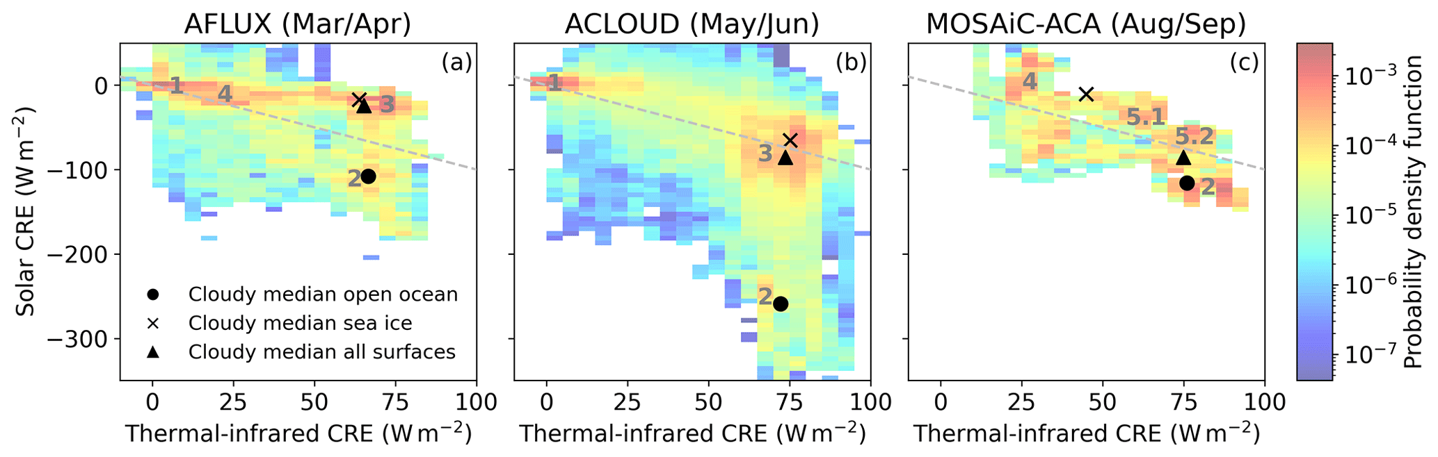
Figure 9 Two-dimensional probability density function of CRE_sol and CRE_TIR for (a) AFLUX , (b) ACLOUD, and (c) MOSAiC-ACA. The diagonal dashed lines represent the 0 W m⁻² isoline of CRE_tot. The symbols represent the median of CRE_sol and CRE_TIR over the surface types given in the legend in panel (a) and only considering cloudy observations (equivalent LWP > 5 g m⁻²). The numbered modes represent (1) cloud-free, (2) cloudy open ocean, (3) cloudy sea ice, (4) thin/broken clouds, and (5.1/5.2) cloudy MIZ conditions.

The median CRE_TIR observed in cloudy conditions during AFLUX was 67 W m⁻² over open ocean and 64 W m⁻² over sea ice. The slightly lower value for the latter was caused by the enhanced frequency of observations with relatively low CRE_TIR (< 30 W m⁻²), which might be linked to the larger fraction of thin clouds (Fig. 3a) or to the slightly lower cloud base temperature (Fig. 2) over sea ice. For AFLUX, a cloud base temperature change of 1 K results in a change of CRE_TIR in the order of 4 W m⁻², which is approximately the difference between the median CRE_TIR over sea ice and open ocean.

During ACLOUD (Fig. 8b and e), cloud-free conditions were significantly less frequent over open ocean than over sea ice. Instead, the distribution of open ocean reveals an additional small mode around 25 W m⁻². CRE_TIR in cloudy conditions did not differ significantly between the surface types, with median values ranging between 72 W m⁻² over open ocean and 75 W m⁻² over sea ice. The slightly stronger CRE_TIR over sea ice cannot be explained by the cloud base temperature (Fig. 2), which showed lower values over sea ice. Likely, the more frequent occurrence of thick clouds (Fig. 3b) caused this tendency. Also compared to AFLUX, the thicker clouds during ACLOUD are likely the reason for the stronger CRE_TIR, since the increased absolute humidity counteracts the effect of the higher cloud base temperature during ACLOUD (Cox et al., 2015). Except for the additional small mode for open ocean, the cloud-free and cloudy modes are more clearly separated during ACLOUD compared to AFLUX.

Similar to CRE_sol, the low amount of data obtained during MOSAiC-ACA results in a less significant mode structure (Fig. 8e and f). Only in the distribution of open ocean are two distinct modes visible. Due to the lack of cloud-free observations, the mode with the smallest CRE_TIR represents the broken cloud conditions (around 25 W m⁻²). However, these observations mostly coincide with an equivalent LWP of less than 5 g m⁻² and do not significantly contribute to the median CRE_TIR of 75 W m⁻² in cloudy conditions over open ocean. This median value is similar to the median CRE_TIR obtained during ACLOUD, which is probably due to the similar frequency of thick clouds (Fig. 3). Over sea ice, a significantly weaker CRE_TIR was observed during MOSAiC-ACA (45 W m⁻²), which results from the limited sampling statistics. Nevertheless, this is in agreement with the lower observed cloud base temperature (Fig. 2) and the significantly thinner clouds (Fig. 3c).

4.3 Total cloud radiative effect

The previous analysis showed that the variability of CRE_TIR between the campaigns and the surface types is significantly lower than the variability of CRE_sol. Thus, the latter is the major driver of the variability of CRE_tot. Depending on whether the solar cooling or the TIR warming effect dominates, CRE_tot determines whether a cloud has a cooling or a warming effect on the surface. Figure 9 illustrates two-dimensional frequency distributions, combining CRE_sol and CRE_TIR to assess CRE_tot. All modes visible in Fig. 9 can be attributed to the modes discussed in Figs. 7 and 8. In the distributions of AFLUX (Fig. 9a) and ACLOUD (Fig. 9b), mode 1 is clustered around 0 W m⁻² for both CRE_sol and CRE_TIR and combines the mostly cloud-free observations over open ocean and sea ice. The clearly distinct CRE_sol over the different surface types (Fig. 7) separates the cloudy modes over open ocean (mode 2, stronger solar cooling effect) and sea ice (mode 3), while CRE_TIR is similar.

Over open ocean (mode 2), clouds of sufficient LWP showed a total cooling effect (negative CRE_tot, values below the dashed line in Fig. 9) during all campaigns. However, the magnitudes of CRE_tot differed significantly, as quantified by the median values of −48, −185, and −36 W m⁻² during AFLUX, ACLOUD, and MOSAiC-ACA, respectively. Due to the lower SZA during ACLOUD, the solar cooling effect dominated CRE_tot. Over sea ice, the TIR warming effect was dominant over the solar cooling effect during AFLUX, resulting in a median CRE_tot of 42 W m⁻². During ACLOUD, however, CRE_sol and CRE_TIR roughly compensated, leading to a small median CRE_tot of 7 W m⁻².

During AFLUX, a significant amount of observations ranges in a transition between modes 1 and 3. These data correspond to the observations over sea ice with low CRE_TIR that were already discussed in Fig. 8a. The clouds during these situations were rather thin, with a median equivalent LWP of 19 g m⁻² compared to 54 g m⁻² for the observations forming the cloudy sea ice mode (mode 3). The almost absent solar cooling in combination with a TIR warming leads to the total warming effect of these thin clouds often discussed in literature (e.g. Miller et al., 2015), which under certain circumstances can induce ice melting (Bennartz et al., 2013).

Again, the sparse statistics during MOSAiC-ACA need to be interpreted with caution and represent only a subsample of possible cloud conditions (Fig. 9c). Instead of the cloud-free mode (mode 1) observed for the other campaigns, mode 4 represents the broken clouds that produced only a slightly positive CRE_sol but a significantly positive CRE_TIR, with median values of 7 and 26 W m⁻², respectively. The resulting positive CRE_tot underlines that the warming effect of broken clouds can also be observed over open ocean. Modes 5.1 and 5.2 reveal a cloud warming effect over the MIZ, while a separate sea ice mode is missing.

For the regional average CRE_tot, the sea ice concentration within the area of observations is most relevant. While the sea ice situation in the Fram Strait north-west of Svalbard was similar during AFLUX and ACLOUD (Fig. 1a and b), the sea ice edge was located significantly further north during MOSAiC-ACA (Fig. 1c), and the MIZ was broader. This also affected the fraction of observations obtained for each of the surface types and determined the strength of the different modes in Fig. 9. As a proxy for the entire Fram Strait, the median of CRE_tot observed in cloudy conditions during one single campaign was calculated regardless of surface type (triangles in Fig. 9). For MOSAiC-ACA, this median CRE_tot of −27 W m⁻² was close to the median for open ocean due to the dominance of this surface type. During AFLUX, a positive median CRE_tot of 25 W m⁻², and during ACLOUD, a negative median CRE_tot of −16 W m⁻² was observed, both ranging close to the median values of sea ice. Given the different SZA ranges during both campaigns, this indicates that clouds over the Fram Strait showed a warming effect at the surface during AFLUX (spring) and an almost neutral to slightly negative CRE_tot during ACLOUD (early summer). MOSAiC-ACA revealed a similar median of CRE_tot compared to AFLUX for the individual surface types. However, the dominant open-ocean surfaces during MOSAiC-ACA caused the clouds to have an average cooling effect during late summer.

5 Conclusions

To compare the warming or cooling effects of clouds over sea ice and open ocean during different times of the year, the surface CRE was evaluated from observations performed during three campaigns in the Fram Strait north-west of Svalbard. The campaigns AFLUX, ACLOUD, and MOSAiC-ACA were characterized by significantly different sea ice coverages and thermodynamic states during spring, early summer, and late summer, respectively. The CRE was calculated from a combination of airborne broadband radiation measurements and radiative transfer simulations. While F_net,sol,cld and F_net,TIR,cld were measured during low-level flight sections, the corresponding F_net,sol,cf and F_net,TIR,cf were simulated and accounted for changes of the surface albedo between cloudy and cloud-free conditions (Stapf et al., 2020). This was done by retrieving the cloud-free surface albedo from parameterizations for sea ice and open-ocean surfaces. The radiative impact of clouds on the surface albedo differed between the surface types and was not uniform among the different campaigns.

CRE_sol and CRE_tot were affected distinctly by these cloud-induced differences of the surface albedo, mainly depending on the SZA. The consideration of this effect almost doubled CRE_sol over sea ice during ACLOUD, as already discussed by Stapf et al. (2020). In contrast, the larger SZAs present during the other campaigns suppressed similar changes of CRE_sol. However, over open ocean, the impact of the cloud-induced albedo change increases with increasing SZA. Thus, the solar cooling effect over open ocean was weakened by about 20 % during MOSAiC-ACA, while ACLOUD was not affected. During AFLUX, the albedo change was masked by the presence of sea smoke.

CRE_sol strongly varied between sea ice and open-ocean surfaces as well as among the campaigns. While the low surface albedo caused a strong solar cooling effect over open ocean, the cooling effect over sea ice was rather weak and partly not distinguishable from cloud-free conditions. This weak cooling was often supported by the presence of thin clouds. Due to the lower SZA, CRE_sol showed a significantly stronger cooling effect during ACLOUD compared to the other campaigns.

The variability of CRE_TIR results from a complex interplay between changing thermodynamic and cloud properties. In contrast to CRE_sol, CRE_TIR varied only weakly between the surface types and the campaigns and mostly showed median values between 64 and 76 W m⁻². Compared to the other campaigns, a weaker CRE_TIR was found during AFLUX, which was caused by the enhanced frequency of optically thin clouds.

The variability of CRE_tot is driven by CRE_sol. A negative CRE_tot, dominated by the solar cooling effect, was found over open ocean during all campaigns. This cooling effect was strongest during ACLOUD (−185 W m⁻²) compared to the other two campaigns (around −40 W m⁻²). Over sea ice and the MIZ, the warming effect of CRE_TIR clearly dominated during AFLUX (42 W m⁻²) and MOSAiC-ACA (22 W m⁻²), while CRE_sol and CRE_TIR roughly compensated during ACLOUD. Broken and optically thin clouds showed a total warming effect, independent of the underlying surface. This is due to their almost neutral to slightly positive CRE_sol and their significantly positive CRE_TIR. In addition to the SZA, CRE_tot not separated for the surface types differs between the campaigns due to the seasonally different sea ice distributions. For each campaign, the sea ice distribution in the Fram Strait region is imprinted in the fraction of observations over the respective surface types. The high fraction of observations over sea ice during AFLUX and ACLOUD implies a warming and almost neutral effect of clouds in the Fram Strait during spring and early summer, respectively. In contrast, the frequent observations over open ocean during MOSAiC-ACA cause a cooling effect of clouds in the Fram Strait during late summer.

The short low-level flight segments during the campaigns are not necessarily representative of an entire season from a climatological point of view. The results might be biased by the flight strategy and the spatial and temporal selection of low-level sections to satisfy different campaign goals. Furthermore, not all synoptic conditions could be captured due to weather-caused flight limitations. To overcome these limitations and to improve the statistics of the surface CRE, extensive low-level sections are necessary regardless of the weather conditions. However, various CRE differences between the campaigns could be attributed to their seasonality. Although observations of annual cycles of the CRE over sea ice are available (e.g. SHEBA, MOSAiC), the lack of long-term observations over open ocean complicates a robust characterization of the CRE. This especially holds since ice-free conditions will likely become more dominant in the future Arctic. The validation of satellite CRE retrievals with airborne measurements might be the key for long-term observations of the CRE over open ocean. This study and the published data sets of the CRE in the Fram Strait (Stapf et al., 2021c; Becker et al., 2023) could provide a basis for such investigations and for further research of cloud-related processes and feedback mechanisms in numerical models. Nevertheless, the predominant cooling effect of clouds over open ocean will likely lead to a negative contribution to further warming in the Arctic.