the Creative Commons Attribution 4.0 License.
the Creative Commons Attribution 4.0 License.
 | 12 Jun 2023
Development of a CMAQ–PMF-based composite index for prescribing an effective ozone abatement strategy: a case study of sensitivity of surface ozone to precursor volatile organic compound species in southern Taiwan
Jackson Hian-Wui Chang
Stephen M. Griffith
Steven Soon-Kai Kong
Ming-Tung Chuang
Neng-Huei Lin
Photochemical ozone pollution is a serious air quality problem under weak synoptic conditions in many areas worldwide. Volatile organic compounds (VOCs) are largely responsible for ozone production in urban areas where nitrogen oxide (NOx) mixing ratios are high while usually not a limiting precursor to ozone (O3). In this study, the Community Multiscale Air Quality model higher-order decoupled direct method (CMAQ-HDDM) at an urban-scale resolution (1.0 km×1.0 km) in conjunction with positive matrix factorization (PMF) was used to identify the dominant sources of highly sensitive VOC species to ozone formation in southern Taiwan, a complex region of coastal urban and industrial parks and inland mountainous areas. First-order, second-order, and cross sensitivities of ozone concentrations to domain-wide (i.e., urban, suburban, and rural) NOx and VOC emissions were determined for the study area. Negative (positive) first-order sensitivities to NOx emissions are dominant over urban (inland) areas, confirming ozone production sensitivity favors the VOC-limited regime (NOx-limited regime) in southern Taiwan. Furthermore, most of the urban areas also exhibited negative second-order sensitivity to NOx emissions, indicating a negative O3 convex response where the linear increase of O3 from decreasing NOx emissions was largely attenuated by the nonlinear effects. Due to the solidly VOC-limited regime and the relative insensitivity of O3 production to increases or decreases of NOx emissions, this study pursued the VOC species that contributed the most to ozone formation. PMF analysis driven by VOCs resolved eight factors including mixed industry (21 %), vehicle emissions (22 %), solvent usage (17 %), biogenic sources (12 %), plastic industry (10 %), aged air mass (7 %), motorcycle exhausts (7 %), and manufacturing industry (5 %). Furthermore, a composite index that quantitatively combined the CMAQ-HDDM sensitivity coefficient and PMF-resolved factor contribution was developed to identify the key VOC species that should be targeted for effective ozone abatement. Our results indicate that VOC control measures should target (1) solvent usage for painting, coating and the printing industry, which emits abundant toluene and xylene; (2) gasoline fuel vehicle emissions of n-butane, isopentane, isobutane, and n-pentane; and (3) ethylene and propylene emissions from the petrochemical industry.
- Article
(11493 KB) - Full-text XML
-
Supplement
(2825 KB) - BibTeX
- EndNote


Photochemical production of tropospheric ozone (O3) depends in a nonlinear manner on the availability of nitrogen oxides (NOx) and volatile organic compounds (VOCs). Understanding ozone formation sensitivity to NOx and VOC emissions is key to developing effective abatement strategies on O3 pollution in heavily polluted cities. The brute-force method (BFM) has often been used to address the relationship between O3 and its precursors (Hakami et al., 2004b; Li et al., 2013a; Zhang et al., 2009). In a BFM approach within a 3D-modeling framework (e.g., Community Multiscale Air Quality modeling system – CMAQ), individual emissions are perturbed by a small amount, and the model response is recorded against the baseline, representing the sensitivity coefficient. However, the linear response of BFM is insufficient to account for changes in secondary pollutants (i.e., ozone) generated by nonlinear interactions of various substances. Therefore, more sophisticated numerical techniques have been introduced such as the adjoint method (Hakami et al., 2006; Wang et al., 2021); the decoupled direct method in three dimensions, DDM 3D (Dunker et al., 2002b; Luecken et al., 2018); and the higher-order decoupled direct method, HDDM 3D (Cohan et al., 2005; Koplitz et al., 2021), where the 3D aspect is specific to implementation in chemical transport models (CTMs) with a 3D-modeling framework (e.g., CMAQ). These methods offer an alternative to BFM by directly solving the auxiliary equations that represent the change in concentration over change in emission () derived from the governing equations of the model.
DDM 3D, using a semi-implicit finite-difference scheme with different time steps (Hakami et al., 2004a; Yang et al., 1997), has been widely implemented in CTMs (Dunker et al., 2002b, a) to calculate the first-order sensitivities (i.e., tangential, ) of ozone with respect to initial concentration, boundary concentrations, and precursor emission rates. First-order sensitivity describes the linear response of the model to a perturbed input parameter, while higher-order sensitivity describes the nonlinear quadratic, cubic, and higher-power responses. In the presence of strong nonlinearity (e.g., in the transition between the VOC-limited and NOx-limited regime), first-order sensitivity alone may be insufficient to characterize the response if the magnitude of the emission changes are large (i.e., a manifestation of the nonlinear chemistry involved in ozone formation), and second-order sensitivity is necessary to provide the additional nonlinear responses of the system (Xing et al., 2011; Xiao et al., 2010). Thus, in HDDM, the sensitivity is calculated by solving the first-order () and second-order (i.e., local slope, ) derivatives in the model when a relative perturbation (e.g., ±10 %) is applied to a targeted parameter while keeping all other factors constant.
Apportioning pollutant concentrations to their sources is an ideal strategy to guide emission control policy (Dunker et al., 2015; Liu et al., 2008). However, source apportionment of a secondary pollutant such as ozone is complex, where a relatively crude method is to simply conduct simulations with and without NOx and VOC emissions from a given source so that the difference in ozone concentration is a measure of the source contribution (Bergin et al., 2008). Other source apportionment approaches such as the ozone source apportionment technology (OSAT) and integrated source apportionment method (ISAM) are embedded into air quality models (Comprehensive Air Quality Model with Extensions (CAMx) and CMAQ, respectively) and rely on tagging NOx and VOCs as tracers from emission to ozone production to estimate the contributions of different sources to the eventual ozone concentration (Dunker et al., 2002a; Kwok et al., 2015). Unless a high-resolution sector profile emission inventory is available, the application of OSAT and ISAM is often limited to four main sector groups: on-road, non-point (area), point, and biogenic sources (Wang et al., 2009; Li et al., 2013b). In addition, the spatiotemporal and sector group distribution uncertainties associated with the emission inventory greatly influence the accuracy of these source apportionment methods (Zheng et al., 2009).
Positive matrix factorization (PMF), a receptor-based approach, offers an alternative to those embedded methods by generating a set of ozone precursor source composition profiles, each identifying a mix of compounds associated with a particular category of emissions. Driven by measured concentrations at receptor sites, PMF can be used as an ozone source apportionment method directly and is independent of the uncertainties associated with the emission inventory. In recent years, PMF has been widely used to estimate VOC apportionment because it requires only identifying characteristics of the source profiles to interpret the PMF factors (Ji et al., 2022; Fan et al., 2021; Huang and Hsieh, 2020; Chen et al., 2019; Wu et al., 2016). For instance, Pallavi et al. (2019) found that traffic contributed 47 % of the total benzene in India followed by residential biofuel use and waste disposal (25 %) and industrial emissions and solvent use (20 %). Zhao et al. (2020) used PMF in conjunction with an ozone formation potential (OFP) calculation to infer that VOCs from industrial and vehicular emissions were the dominant ozone precursors in Nanjing, East China, particularly xylenes, toluene, and propene. Chen et al. (2019) used PMF to resolve the dominant VOC sources at an industrial complex in central Taiwan and found that the monitored VOC concentrations of vehicle exhaust, solvent use, and diesel attributed to high OFP were associated with easterly to southeasterly winds. Huang and Hsieh (2020) analyzed VOC data by PMF from western coastal Taiwan and suggested that on a mass concentration basis industrial emissions are the greatest contributors to OFP. However, previous PMF–OFP studies have only identified key VOC sources to OFP without investigating the sensitivity of OFP to these VOC emissions and thus failed to provide comprehensive advice on which sources to prioritize for effective ozone abatement.
In this work, we used CMAQ-HDDM-3D in conjunction with PMF, enabling us to interpret the sensitivity and source apportionment analyses together for a more comprehensive investigation of the key VOC sources to OFP. We combined the two approaches as a novel methodology to provide additional insights on the dominant sources of highly sensitive VOC species to ozone formation in a VOC-limited urban area of Taiwan, but this should be widely applicable across urban areas that experience similar O3 episodes such as Hong Kong (Ling and Guo, 2014); Beijing and Hebei (Chi et al., 2018); Mexico City (Lei et al., 2007); and Houston, United States (Mazzuca et al., 2016). Specifically, HDDM describes the O3 sensitivity response to a speciated emission and PMF identifies the sources of these species for effective ozone abatement strategy. While most of the HDDM sensitivity studies are performed at coarse resolution (>4.0 km), this study was conducted at an urban-scale resolution (1.0 km×1.0 km). We investigated the first-order, second-order, and cross sensitivities of ozone concentrations to domain-wide NOx and VOC emissions and provide an overview of the O3-precursor sensitivity across the study area. We then identified the VOC species to which ozone formation was most sensitive. Finally, we mapped these highly sensitive VOC species to the PMF model source apportionment and identified their dominant sources for effective emission control strategies using a composite index of CMAQ sensitivities and PMF factor contributions. The results of our study provide important information as to which VOC species are key to ozone formation and where to reduce sources of these VOC species for effective ozone abatement.
2.1 Study period and area
In this study, we selected the period from 7–20 October 2018 for conducting simulations of photochemical ozone production and transport in southern Taiwan. The selected case in October 2018 is the seasonal transition period when the summer season is in transition to the winter. The case can reasonably represent the typical ozone pollution conditions during the seasonal transition period in Taiwan because the synoptic weather pattern of the event features a weak intrusion of the Asian continental anticyclone system which slowly propagated eastward, causing the prevailing wind in Taiwan dominated by weak northeasterly (NE) flows due to continental high-pressure peripheral circulation (see Fig. S1 in the Supplement). Hsu and Cheng (2019) identified six synoptic weather patterns common in Taiwan and studied the characteristics of corresponding air pollutants in each pattern using 6 years (2013–2018) of daily averaged wind fields and sea-level pressure observed at surface weather stations in Taiwan. Among the six patterns (C1–C6), C4 has the highest mean O3 concentrations and occurs predominantly in October. It features a weak anticyclone over the Asian continent, and the Pacific subtropical high-pressure system does not have an apparent influence in Taiwan, which is similar to our selected case in October 2018. Although the photochemistry is strong in the summer season, the seasonal O3 variation in Taiwan shows that the monthly O3 concentration is relatively higher during the seasonal transition months (i.e., October) compared to other seasons (Hsu and Cheng, 2019; Chen et al., 2021; Cheng et al., 2015). This is because during the seasonal transition months, when the photochemical reaction is still strong compared to that of the winter months together with the reduced ventilation capability, the O3 concentration can accumulate (Yen and Chen, 2000; Tsai et al., 2008) (see Fig. S2 in the Supplement for ozone seasonality in Taiwan). During the seasonal transition period in autumn, southern Taiwan often suffers from high-O3 episodes (Hsu and Cheng, 2019; Chen et al., 2004, 2021). Regional synoptic weather in autumn usually features a weak anticyclone over the Asian continent, allowing for local accumulation of pollutants, while the Pacific subtropical high-pressure system has shifted eastward with no apparent influence on Taiwan (Hsu and Cheng, 2019). This synoptic weather pattern is also categorized as high-pressure pushing (HPP), which occurred when the leading edge of Asian continental high-pressure systems moves over China coastal provinces and carries pollutants southward towards downwind area in Taiwan (Chuang et al., 2008). In addition, precipitation is lower and vertical dispersion is weaker than in summer (Yen and Chen, 2000; Tsai et al., 2008), which contribute to relatively more frequent ozone episodes in autumn. These conditions are also common occurrences for high-O3 episodes in other places such as Hong Kong and East China cities in autumn (Lee et al., 2009; Liu et al., 2021; R. Yu et al., 2021). A 5 d spin-up period (2–6 October 2018) was discarded from the analysis to eliminate the effects of initial conditions on O3 simulations.
Since the 1990s, ozone concentrations have been increasing in many areas of southern Taiwan (Chang et al., 2005; Chen et al., 2021). Kaohsiung city, the biggest city in southern Taiwan and second biggest in all of Taiwan, hosts many heavy industries, including petrochemical plants, refineries, steel-making plants, and power generation plants. Xiaogang (XG) district is located in the southeastern portion of the city and hosts a petrochemical industrial park with an overall area of 403 ha. Three power plants, each producing 1200–4300 MW d−1, are located within a distance of 35 km of XG and lead to some of the poorest air quality in Taiwan.
2.2 WRF–CMAQ model configuration
The Weather Research and Forecasting (WRF) model version 3.9.1 and CMAQ model version 5.2.1 (WRF–CMAQ) is used in the current study with a domain configuration of a four-nested grid system centered at 28∘ N and 125∘ W (Fig. 1a). The outermost domain (D01) covers most of mainland China with a horizontal resolution 27 km×27 km and 166×169 grids, which is then nested to the second domain (D02) of 9 km×9 km and 223×223 grids over East China. The third domain (D03) covers the whole island of Taiwan with a resolution of 3 km×3 km and 223×223 grids, and the innermost domain (D04) focuses on southern Taiwan with a 1 km×1 km resolution and 136×136 grids. There are 41 vertical sigma layers spaced unequally from the ground to the model top 50 hPa, with the bottom 8 layers resolved below 1.5 km (Fig. S3 in the Supplement).
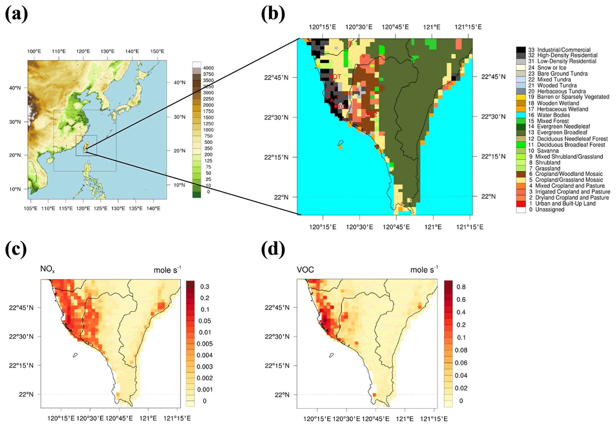
Figure 1(a) Domain configuration of a four-nested grid system; (b) land use of the innermost domain; urban and inland areas are represented by class 31, 32, 33, and 6, respectively, (c, d) monthly averaged NOx and VOC emissions in the innermost domain obtained from the 2016 TEDS-10 emission inventory. The locations of each TEPA air quality station (red stars) and PAMS station (red dots with label) used in the current study are displayed in the innermost domain. Refer to Fig. S3 and Table S3 in the Supplement for details of each TEPA and PAMS station.
The initial and boundary meteorological conditions are adopted from the National Centers for Environmental Prediction (NCEP) global final analysis (FNL) data at resolution updated every 6 h. The projected 2017-year Multi-resolution Emission Inventory for China (available at http://meicmodel.org, last access: 30 January 2022) with resolution is used for D01 and D02, while the 2016 Taiwan Emission Data System (TEDS) version 10 (Fig. 1c and d) is used for D03 and D04. Biogenic emissions are calculated offline using the Model of Emissions of Gases and Aerosols from Nature (MEGAN) version 2.10 (Guenther et al., 2006).
Other than local anthropogenic emissions, the contribution of long-range transport (LRT) from East Asia (e.g., Chinese emissions) is also substantial to Taiwan's air quality, especially under strong northeasterly wind conditions (Wu and Huang, 2021; C.-T. Chang et al., 2022). Lin et al. (2004) identified three types of common LRT events in Taiwan: (1) dust storm (DS), (2) LRT with pollutants (frontal pollution; FP), and (3) LRT of background air masses (BG). When there is no frontal system, local pollution (LP) dominates the air quality in Taiwan. During wintertime and springtime, the occurrence of LP cases was 70 %, and about 30 % were LRT cases (Lin et al., 2004). Lin et al. (2005) estimated that the long-range transport of pollutants contributes to about 30 µg m−3, 230 ppb, and 0.5 ppb to the PM10, CO, and SO2 concentrations, respectively, in northern and eastern Taiwan. Meanwhile a smaller contribution is estimated in southern Taiwan due to the geography (Lin et al., 2005).
In our work, the oceanic chlorine emission is calculated online by CMAQ as a function of meteorology using an OCEAN file which specifies the fraction of each grid cell that is open ocean (OPEN) or surf zone (SURF). Figure 2a–c present the spatial distribution of CMAQ-calculated sea-salt aerosol cations (ASEACAT – Na+, K+, Ca2+, and Mg2+), fine-mode chlorine, and coarse-mode chlorine emission rates averaged during the entire simulation period. The sea-spray emissions were higher in the surf zone area, and the highest emission rates were found along the eastern offshore area of southern Taiwan. This is because of the enhanced formation of sea-spray aerosols associated with higher relative humidity and greater offshore winds along the eastern offshore area of southern Taiwan that is open to the western Pacific Ocean. Besides, the anthropogenic chlorine (PCL) emissions are obtained from TEDS v10 emissions, and they are concentrated over the heavily industrialized urban areas of southern Taiwan (see Fig. 2d).
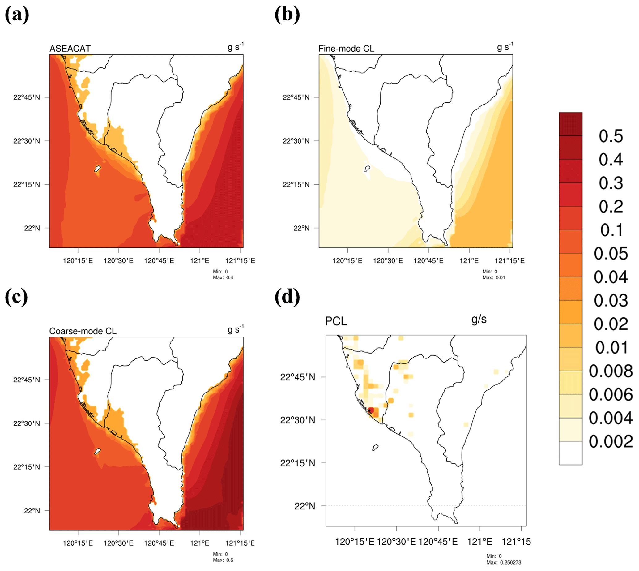
Figure 2CMAQ-calculated (a) sea-salt aerosol cation (ASEACAT) emissions (Na+, K+, Ca2+, and Mg2+), (b) fine-mode chlorine sea-spray aerosol (SSA) emissions, (c) coarse-mode chlorine SSA emissions, and (d) TEDS v10 anthropogenic chlorine (PCL) emissions averaged during the entire simulation period.
To obtain more accurate dynamical downscaling, grid nudging was applied in the coarse domains D01 and D02; observation nudging was applied in the fine domains D03 and D04. Grid nudging is applied to the horizontal wind components, potential temperature, and water vapor mixing ratio; it is only applied above the planetary boundary layer (PBL). The observational data for observation nudging include hourly surface observations such as atmospheric pressure, air temperature, relative humidity, wind speed, and wind direction from 36 surface meteorological stations (https://www.epa.gov.tw/, last access: 30 January 2022), as well as the twice-daily at 00:00 and 12:00 UTC sounding data such as potential height, temperature, dew point temperature, RH, wind direction, and wind speed at each specified isobaric level from two radiosonde observation stations in Taiwan. The nudging coefficients, which determine the strength of the assimilation tendency term, were set to be for observation nudging and for grid nudging. These values of coefficients were recommended by the WRF user guide and tested to be appropriate in previous studies (Li et al., 2022; Borge et al., 2008).
The simulation adopted the Carbon Bond Mechanism CB6 (Yarwood et al., 2010), which was developed as an update to CB05 to provide a condensed chemical mechanism for use in atmospheric models. CB6 includes five additional organic compounds that are long-lived and relatively abundant (i.e., propane, acetone, benzene, ethyne, and higher ketones) and a more detailed representation of organic nitrate reactions. CB6 has been tested against measurements over a wide variety of spatial, temporal, chemical, and meteorological conditions and has shown good agreement with measurements of ozone and nitrogen oxides in both urban and rural areas (Luecken et al., 2019). The halogen chemistry in CB6 considers chlorine-related reactions such as ClNO2, HCl, and HNO3 production from heterogeneous uptake of N2O5 on the aerosol surface, which are important to ozone pollution over coastal cities in southern Taiwan.
The Noah land surface model (LSM) is used to describe the land–atmosphere interaction (Chen and Dudhia, 2001). The urban effect in Noah LSM is invoked by implementing a single-layer urban canopy model (UCM), which assumes infinitely long 2D street canyon urban geometry to improve the processes associated with the exchange of momentum, heat, and moisture in the urban environment (Kusaka and Kimura, 2004; Kusaka et al., 2001). To take full advantage of the UCM scheme, three additional urban classes (i.e., low-density residential, high-density residential, and industrial/commercial) are further classified for better representation of the urban features (Fig. 1b).
The asymmetric convective model version 2 (ACM2) boundary layer scheme is selected to represent the boundary layer process (Pleim, 2007). It includes the nonlocal scheme of the original ACM combined with an eddy diffusion scheme. Thus, ACM2 is able to represent both the supergrid- and subgrid-scale components of turbulent transport in the convective boundary layer. Also used were the Goddard Cumulus Ensemble (GCE) microphysics scheme (Tao et al., 2014), Rapid Radiative Transfer Model (RRTM) longwave radiation scheme (Gallus and Bresch, 2006), Goddard shortwave radiation scheme (Chou and Suarez, 1999), Monin–Obukhov similarity scheme, and Kain–Fritsch cumulus parameterization scheme (only at D01 and D02).
The modeled results of both meteorology (i.e., 2 m temperature, wind speed and direction, and relative humidity) and air quality (i.e., ozone, nitrogen oxides, and volatile organic compounds) are validated against 15 Taiwan Environmental Protection Administration (TEPA) air quality stations. Overall, the modeling system reproduced the observed meteorological and air quality conditions within the benchmark values (see Supplement – “Model Evaluations”).
The urban and inland grid cells are defined according to the USGS-24 land use category. The urban area is represented by class 1 – urban and built-up land, which we further classified into class 31, 32, and 33 (see Fig. 1b) for the WRF single-layer urban canopy model (SLUCM) simulation. We refer the readers to our previous work for detailed discussion on the land use classification and SLUCM implementation in J. H. W. Chang et al. (2022). The inland area is represented by class 6 – cropland/woodland mosaic (see Fig. 1b). The general meteorological pattern of the event features a weak intrusion of the Asian continental anticyclone system which slowly propagated eastward, causing the prevailing wind at a synoptic scale in Taiwan dominated by weak northeasterly (NE) flows due to continental high-pressure peripheral circulation (see Fig. S1). At a local scale in southern Taiwan, the steering of weak NE flows by the orographic effect of the Central Mountain Range (CMR) enhanced the local circulations (i.e., land–sea breeze) and eventually pushed the locally produced urban O3 as well as its precursors NOx and non-methane hydrocarbon (NMHC) towards the inland areas (see Fig. 3).
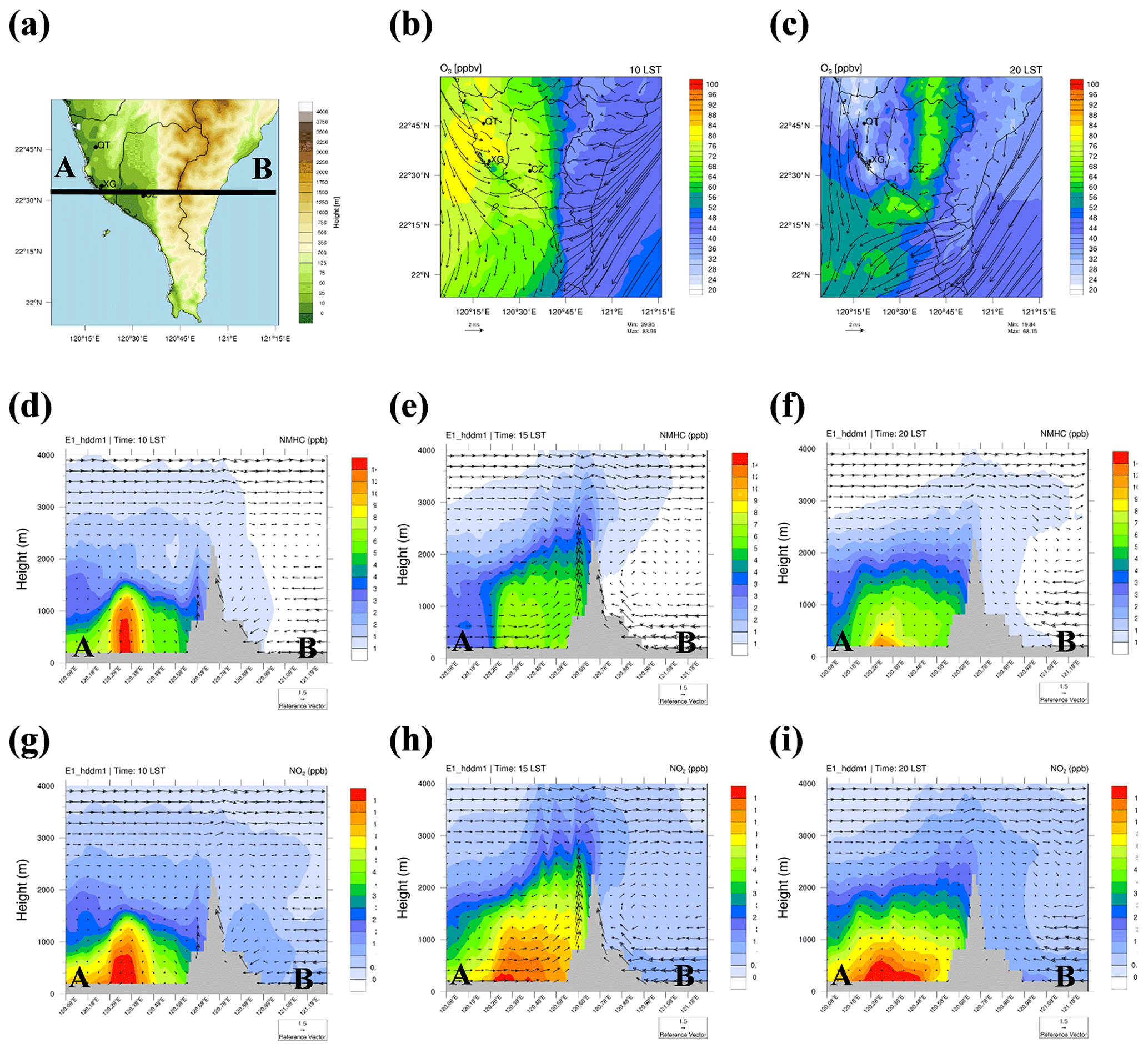
Figure 3(a) Topography of the innermost domain. (b, c) Spatial distribution of O3 concentration averaged during the entire simulation at 10:00 and 20:00 LST, respectively. (d–f) Vertical profile of NMHC concentration cross sectioned at AB (see Fig. 3a) averaged during the entire simulation at 10:00, 15:00, and 20:00 LST, respectively. (h–i) Same as (d–f) but for NO2 concentration.
2.3 Higher-order decoupled direct method (HDDM)
The response of a chemical concentration to perturbations in model parameters (i.e., emissions, initial condition, boundary condition, and reaction rate constants) can be evaluated through sensitivity analysis. A perturbed sensitivity parameter, pi, is related to the unperturbed sensitivity parameter, Pi, in the baseline simulation as
where εi is a scaling factor with a nominal value of 1.0 when there is no perturbation, and Δεi is a perturbed scaling factor. The response of a chemical concentration, C, against the perturbations in a sensitivity parameter, pi, is defined as the sensitivity coefficient, Si. The first- and second-order sensitivity coefficients, and , are defined as follows:
Both Si(1) and Si,j(2) have the same units as the chemical concentration, C. Si(1) measures the impact of one variable pi on a concentration, C; Si,j(2) measures the impact of another variable pj on a first-order sensitivity, Si(1), which can be used to investigate the second-order cross sensitivity of the system. When i=j, Si,i(2) represents the local curvature of the relationship between a concentration and a single parameter, thus indicating the responsiveness of C to a broad range of pi and describing a nonlinearity of the system. A second-order sensitivity of zero indicates a perfectly linear response, while greater values represent proportionally greater nonlinearity effects. Matching signs of the sensitivities (e.g., positive first order and positive second order) represent a convex response while opposite signs represent a concave response (Fig. S4 in the Supplement). In the context of our study, reduced emission is the focus so a convex response represents a nonlinear ozone concentration decrease with decreasing emissions, and a concave response represents a nonlinear ozone concentration increase with decreasing emissions.
Taylor-series expansion
After determining the sensitivity coefficients, we can apply these coefficients for estimating the concentration changes in emission reduction scenarios based on Taylor-series expansion. The concentration changes from any fractional perturbations in a sensitivity parameter are approximated by (Cohan et al., 2005)
where Ci is the concentration when pi has been perturbed by an amount ΔεiPi. Subscript i represents the targeted emission species (i.e., a NOx or VOC species). When multiple sensitivity parameters are perturbed simultaneously, a second-order Taylor approximation includes the interaction between the two parameters (Cohan et al., 2005):
where Si,j is the cross sensitivity between the two parameters, which differs from the sum of the two sensitivities, Si and Sj.
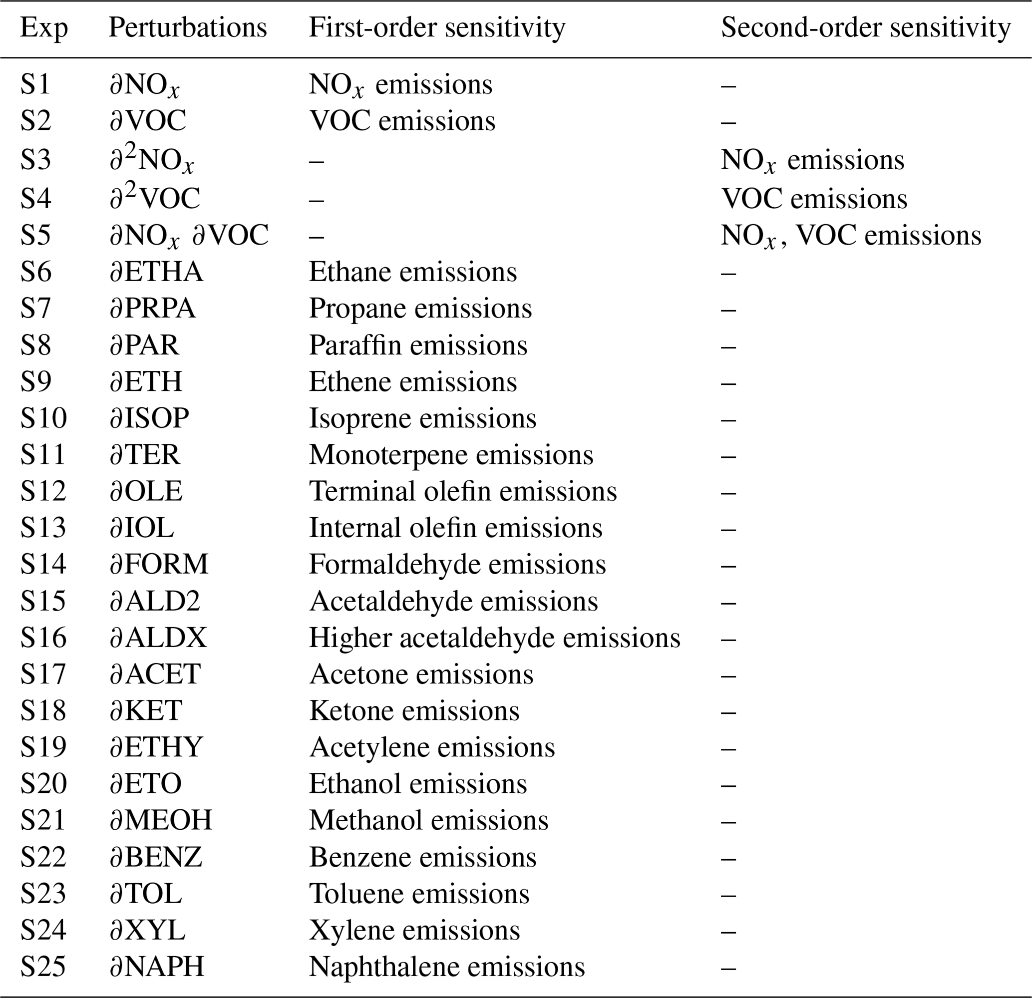
In this study, CMAQ-HDDM-3D v5.2.1 is used to calculate the sensitivity coefficients to predict the O3 response to perturbations in NOx and VOC emissions. Perturbations at ±10 % were made on the domain-wide emissions of NOx and VOCs (D01–D04) from both anthropogenic and biogenic sources, but only sensitivity coefficients from the innermost domain (D04) are used for data analysis. A total of 25 sensitivity tests were performed to quantify the change in O3 concentration due to the perturbations made in each test (Table 1); the first 5 sensitivity tests, S1–S5, account for the first-order, second-order, and cross sensitivity due to the perturbed NOx and total VOC emissions, and the other 20 sensitivity tests, S6–S25, account for sensitivities due to perturbed individual VOC model species. Note that the HDDM approach was only used in experiment S3–S5, which involves calculation of the higher-order sensitivity, while the DDM approach was used in all other experiments and in conjunction with PMF analysis.
Table 1Perturbed emissions considered in the 25 sensitivity tests. The first 5 sensitivity tests S1–S5 account for the first-order, second-order, and cross-order sensitivity due to the domain-wide NOx and VOC emissions, and the other 20 sensitivity tests S6–S25 account for the individual VOC model species.
2.4 Positive matrix factorization (PMF) model
The positive matrix factorization (PMF) model is a source-receptor statistical factor analysis method, which is widely used for apportioning sources of air pollution and resolves the dominant factor profile without prior knowledge of sources; the measured data uncertainty is used to optimize the model (Daellenbach et al., 2017; Fountoukis et al., 2014; Fan et al., 2021). In this study, the US EPA PMF 5.0 receptor model was used for the source apportionment of measured VOC species:
where xij is the jth species concentration measured in the ith sample, gik is the airborne mass contribution from the kth source in the ith sample, fkj is the jth species fraction to the kth source, and eij is the residual associated with the jth species concentration measured in the ith sample. p is the total number of independent sources. Note that the subscript “i” in Eq. (6) refers to the ith sample, which is different from Eqs. (1–5) that refer to the emission of the ith species. In the source parsing process, the objective function Q is solved with an iterative minimization algorithm. The objective function is defined as
where uij is the uncertainty of the jth species in the ith sample.
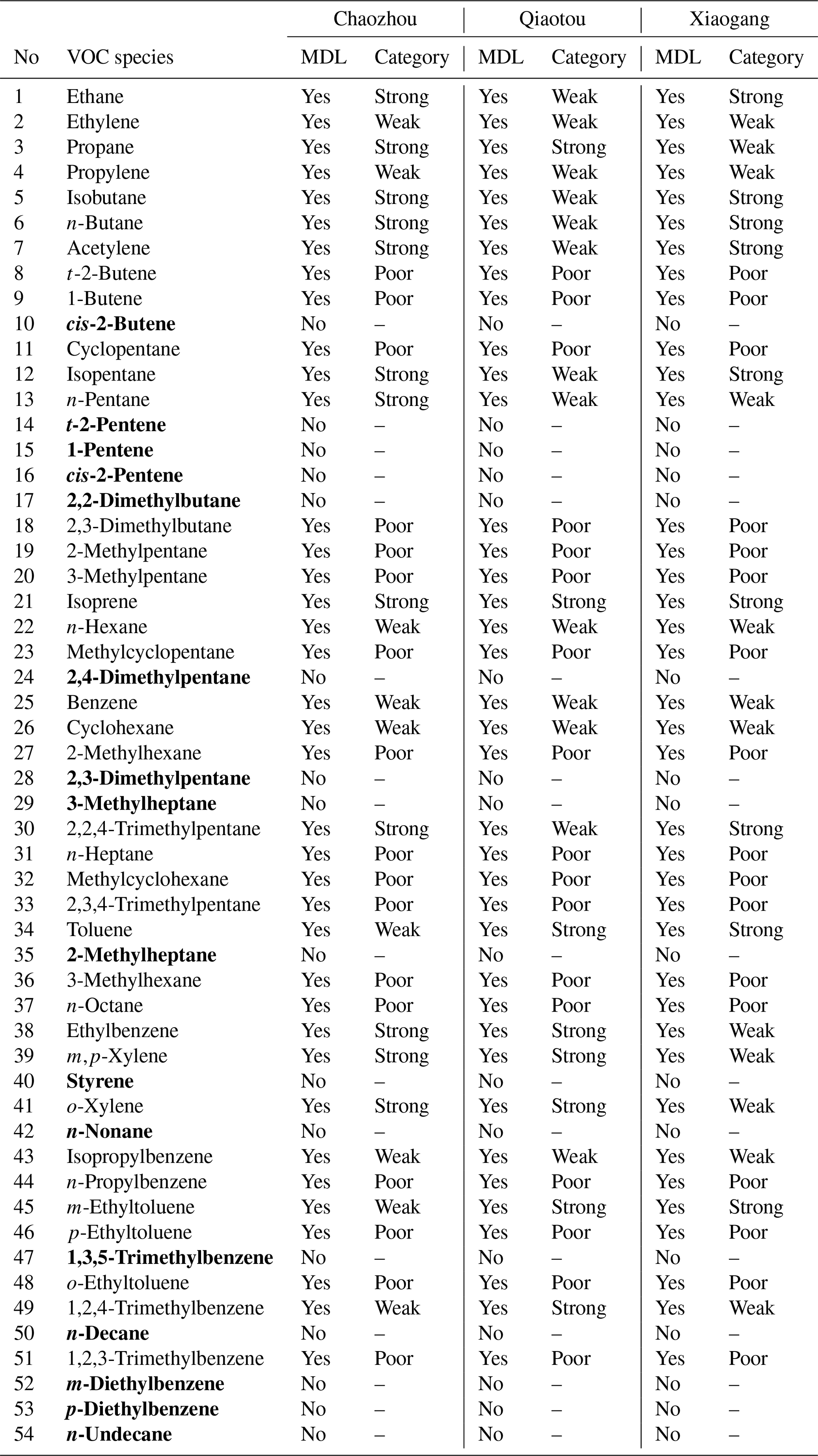
Figure 4 shows the overall framework of the PMF source apportionment methodology. The data used to drive the PMF model source apportionment were obtained from Taiwan's Photochemical Assessment Monitoring Stations (PAMS); details of the PAMS location and sampling protocol are provided in the Supplement. Species with >55 % of samples missing data or below the minimum detection limit (MDL) were discarded (Chen et al., 2019; Wu et al., 2016). Among 54 PAMS-VOC species, a total of 16 species were discarded due to abundant missing data but had a low OFP (Fig. S5 in the Supplement). The sample data uncertainty is calculated using
where MDL represents the minimum detection limit, σ is the error fraction (i.e., 10 % was used in this study), and xij is the concentration of the jth species in the ith sample. In the PMF, we tested a range of three to eight VOC sources to determine the optimal number. Details of this protocol will be discussed further below.
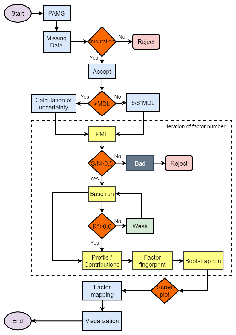
Figure 4Overall framework of the positive matrix factorization (PMF) model methodology. Processes in the dashed-line box are repeated for three to eight factor number combinations. MDL: minimum detection limit.
The Taiwan PAMS data provided a total of 54 VOC species, but not all species were used for the PMF model due to an abundance of values below MDLs. Among the selected 38 VOC species (n=744 samples), they were further categorized into three categories: strong, weak, and poor according to two steps. The first step calculated the signal-to-noise ratio () where species with a value less than 0.5 were classified as poor and removed from the PMF model. This threshold value 0.5 was determined according to the EPA PMF v5.0 user guide and also recommended by other PMF studies (Rajput et al., 2016; Reff et al., 2007). Next, we performed the model base run and calculated the correlation between the modeled and measured concentration for each species. In this step, species with a correlation value ≥0.6 were classified as “strong” and otherwise as “weak”, which were then down-weighted by tripling the analytical uncertainty (Pallavi et al., 2019; Chen et al., 2019). Details of the species categorization are summarized in Table 2. Finally, a total of 21 VOC species were identified and used in the PMF source apportionment analysis, which accounted for 75.0 %, 76.4 %, and 76.1 % of the total VOC concentrations in CZ, QT, and XG, respectively.
Table 2Categorization of PAMS-VOC species for PMF model source apportionment analysis. Bold species represent unused species with abundant missing data >55 % below the minimum detection limit (MDL). Poor category species are identified for low . Weak (Strong) category species are identified for and R2<0.6 (R2≥0.6) between the measured and modeled concentration predicted by the PMF model. Both unused and bad species are removed from the PMF model analysis.
3.1 Decomposition of ozone response
First-order sensitivity coefficients indicate the linear response of ozone concentrations to small changes in emissions. The ozone response to small changes of daytime (09:00–15:00 LST) NOx emissions is dominated by negative sensitivities (VOC-limited) in the urban area and positive sensitivities (NOx-limited) in the inland area near the mountainous region (Fig. 5a). Small areas of extreme negative sensitivity were concentrated near the most intense NOx emissions in XG (magenta borderline in Fig. 5), a heavy industrial park district in the study domain. Although high VOC emissions are also present in the industrial park, the magnitude of first-order sensitivity to NOx emissions (−31 ppb h−1) is relatively larger than that of VOC emissions (+18 ppb h−1), indicating that the O3 linear response to NOx emissions is proportionally greater than that of VOC emissions from the industrial park (see Fig. 5a and b). Moving away from the source emissions, the negative sensitivity to daytime NOx emission gradually increases and becomes positive in the inland area, indicating the shift of ozone production sensitivity from a VOC-limited to NOx-limited regime. The negative sensitivities to daytime NOx emissions extend to the coastal Pingtung county (green borderline in Fig. 5), reflecting the downwind transport of NOx from the source region by the steering of northeasterly winds to westerly winds from the terrain effect and local circulation. Areas of positive sensitivity to VOC emissions overlap with areas of negative sensitivity to NOx emissions, confirming the VOC-limited regime, but also extend to NOx-saturated areas. The larger area of VOC sensitivities could also be explained by the longer atmospheric lifetime of VOCs (hours to days for high-OFP species such as toluene, ethylbenzene, xylene, ethane, and ethylene) as compared to NOx (1.0–4.5 h) (Laughner and Cohen, 2019).
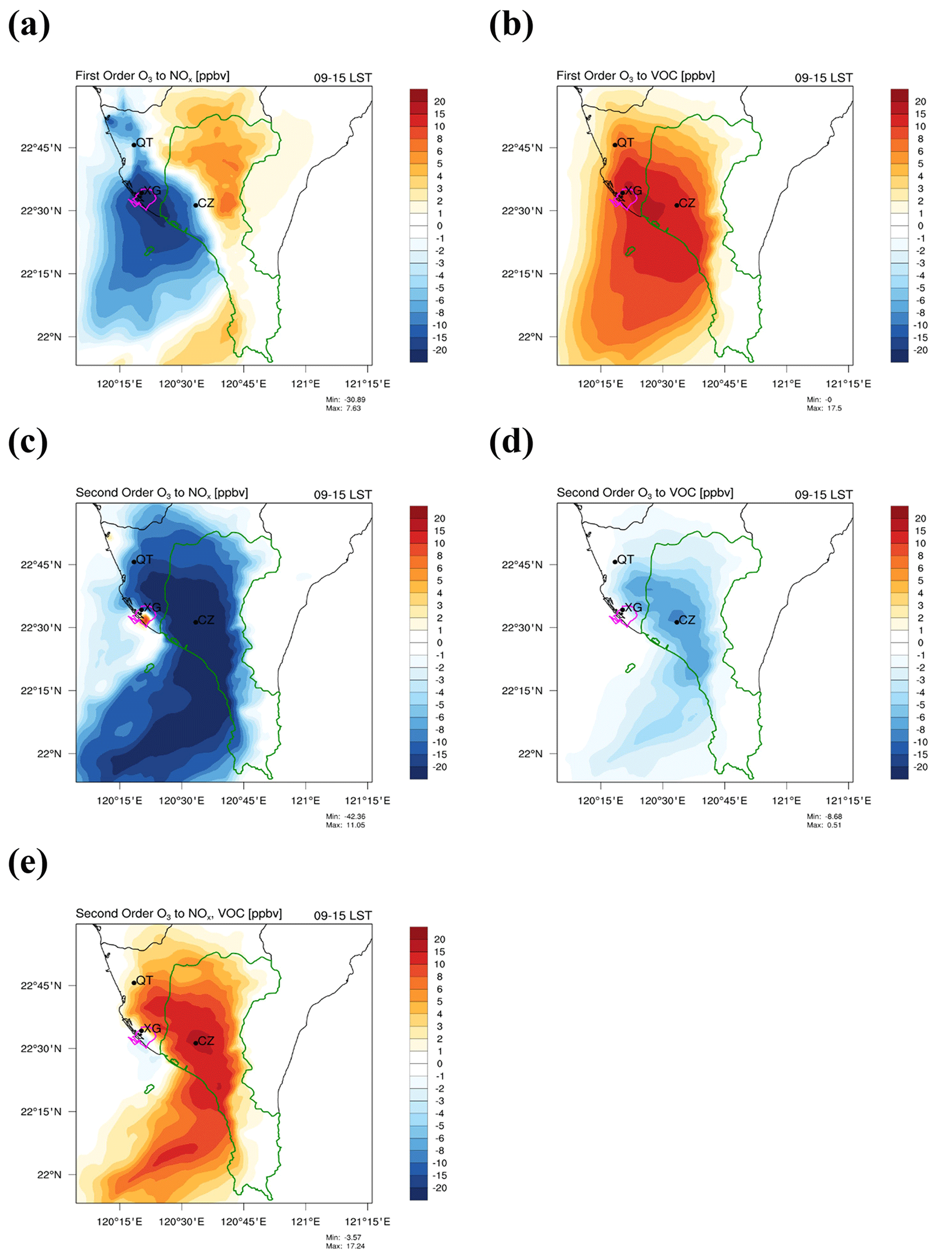
Figure 5CMAQ-HDDM first-order sensitivity coefficient of O3 to (a) NOx emissions, (b) VOC emissions, second-order sensitivity coefficient of O3 to (c) NOx emissions, (d) VOC emissions, (e) second-order cross-sensitivity coefficients of O3 to NOx, VOC emissions, averaged during the entire simulation period at daytime, 09:00–15:00 LST. Magenta and green highlighted borderline represents the Xiaogang district and Pingtung region, respectively.
Second-order sensitivity indicates the responsiveness of ozone concentration to broader changes in emissions and also delineates the nonlinear sensitivities of ozone concentration to emissions. Most of the urban areas (except XG, an industrial park) exhibited negative second-order sensitivities to daytime NOx emissions, which when coincident with negative first-order sensitivities yields a negative O3 convex response: urban O3 increases linearly but decreases nonlinearly with decreasing NOx emissions. Thus, in these areas, the large negative second-order sensitivities countered the linear negative sensitivity of O3 creating urban O3 production conditions that were less sensitive than otherwise to changes in NOx emissions. In contrast, positive second-order sensitivities to daytime NOx emissions in XG were coincident with negative first-order sensitivities, which yielded a negative O3 concave response with linear and nonlinear O3 increases during decreasing NOx emissions (Fig. S2). This concave O3 response is also observed in the Chicago O'Hare (ORD) area, which is highly polluted and severely impacted by aircraft emissions (Arter and Arunachalam, 2021); it is similar to XG where it also hosted an international airport and several industrial parks. In XG, the NOx titration effect that consumes ozone is relatively higher than other urban areas of Kaoping due to the high-NOxVOC conditions (see Fig. S6 in the Supplement), and hence a rapid reduction in NOx level could further suppress the titration effect and increase the ozone formation rate, while for urban areas outside of XG, rapid NOx reductions push the condition into transition or the NOx-limited regime, and suppression of the titration is countered by less efficient O3 production. Cross sensitivities indicate the interaction effects of the sensitivities when both NOx and VOC emissions are changed simultaneously (limited to NOx and VOC changes in the same direction, positive or negative). In most cases, decreasing the NOx (VOC) emissions enhanced the sensitivities of ozone to the limiting precursors, NOx (VOC), due to the positive cross sensitivity of ozone to NOx and VOCs (see Fig. 5e). Cross sensitivities also indicate how results from emission control strategies may change from summing the results of decreasing individual NOx and VOC emissions (Arter and Arunachalam, 2021). Cross sensitivities usually have only a small contribution in highly VOC-limited or highly NOx-limited conditions because the associated net ozone production rates are driven singly either by VOC or NOx, respectively (Sillman, 1999; Cohan et al., 2005). This result is reproduced in our model simulation; low cross sensitivities between NOx and VOC are simulated in XG (highly VOC-limited condition) as well as remote areas in the west side of the mountain range in southern Taiwan (highly NOx-limited condition), while high positive cross sensitivities between NOx and VOC emissions are concentrated in downwind suburban areas (e.g., Pingtung county) (Fig. 5e). The latter result highlights a potential underprediction of O3 formation sensitivity if the cross-sensitivity term is excluded in suburban areas.
3.2 Taylor-series expansion approximation
We then sought to exploit the sensitivity coefficients determined above to estimate the impact of NOx and VOC emission reductions on ozone concentrations in southern Taiwan from the time of our study period, 2018 to 2025. To determine the level of emission reduction in the near term, we referred to the long-term trend of projected emissions in Taiwan as reported in the Taiwan Emission Data System (TEDS 11.0; https://air.epa.gov.tw, last access: 30 January 2022), which estimated an overall reduction of 53 % (NOx) and 14 % (NMHC) over 22 years (2007–2028). In recent years, the decreasing trends for both NOx and NMHC emissions have slowed down (see Fig. S7 in the Supplement). We then used 5 % emission reductions over the 8-year near-term period from 2018–2025 as a conservative estimate. Although this reduction is small, the Taylor-series approximation (Eqs. 4 and 5) considers the first-order, second-order, and cross-sensitivity coefficients of O3 for this change in NOx and VOC emissions and provides a clearer picture on how O3 will change with a parallel reduction in emissions in the near future.
We estimated the ozone concentration at different scenarios represented by different emission control strategies for the typical seasonal transition period already simulated above, which often causes high-O3 episodes in the study area. For simplicity, a reduction of domain-wide NOx and VOC emissions is considered. Given the high nonlinearity of the ozone response to emissions of NOx and VOC, the Taylor-series approximation is necessary to consider the higher-order terms involved in second-order and cross-term sensitivity of NOx and VOC emissions. To compare a series of targeted emission control strategies, four experiments are considered: (1) baseline, (2) NOx control, (3) VOC control, and (4) NOx and VOC control. All experiments reduce the targeted emission by 5 % except for the baseline experiment representing the current emission with no perturbations. Figure 6 shows the baseline O3 concentration and its corresponding response to NOx control, VOC control, and NOx and VOC control at daytime 12:00 LST. Benefits of NOx control (i.e., reduction of O3 by 0.6–0.8 ppbv) are seen to dominate over the inland area. However, an adverse effect of increased O3 concentration >1.8 ppbv from NOx control is simulated near the western coastal urban area where high NOx emissions are concentrated. This agrees with our previous analysis that urban O3 concentrations are estimated to increase from decreasing NOx emissions for most of the urban areas that follow O3 concave sensitivity behaviors and increase more for highly polluted urban areas (i.e., XG) that follow O3 convex sensitivity behaviors. In contrast, no adverse effect is observed from VOC control but rather resulted in decreased O3 concentration over much of the study region. The largest ozone response to VOC control is −1.4 ppbv in the urban area but also extended to the inland area. Control of both NOx and VOC emissions resulted in reduced inland O3 concentration, a marginal difference in urban areas, and slightly increased O3 concentration near the large point source area in XG.
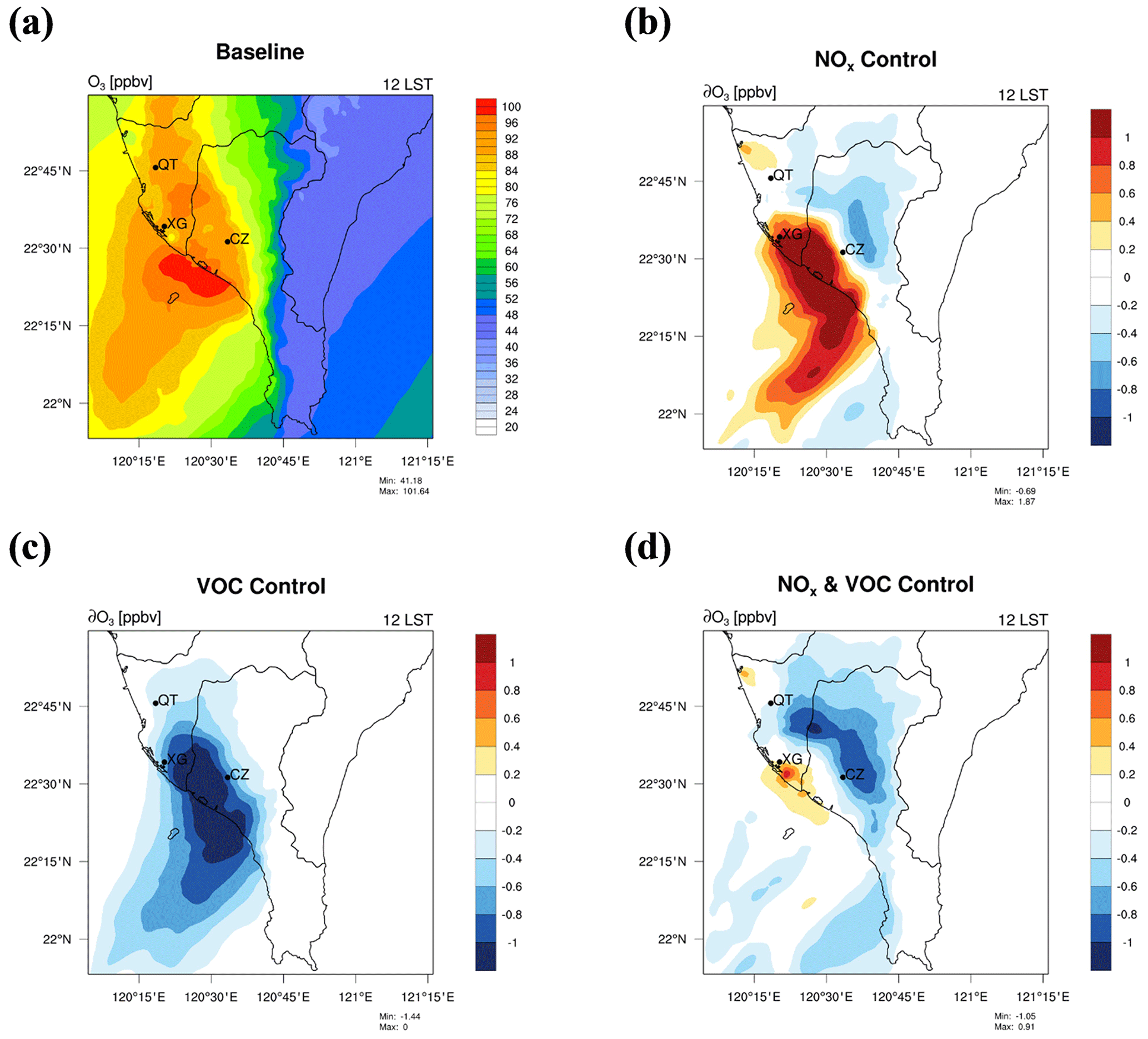
Figure 6Spatial distribution of O3 concentration in (a) the baseline with no perturbations in NOx and VOC emissions, and changes in O3 concentration under the (b) NOx control scenario, (c) VOC control scenario, and (d) NOx and VOC control scenario at daytime 12:00 LST. All scenarios reduced the targeted emissions by 5 % except for the baseline.
The decreasing trend of NOx emission in the future is likely to continue owing to adoption of electric vehicles (EVs), which may impact the urban and inland areas differently due to the respective sensitivity regime. Using the Taylor-series approximation, we estimated ∂O3 against ∂VOC emissions at different levels of projected ∂NOx emissions for Xiaogang, XG (urban), and Chaozhou, CZ (inland), at 12:00 LST (Fig. 7). Projected ∂NOx emissions at 0 % (black line) and −5 % (red line) represent the current year of 2018 and the near future of 2025, respectively, while other projected ∂NOx emissions at arbitrary values of −50 % (blue), −25 % (magenta), and +25 % (green) are presented for alternative scenarios. At CZ, our results show that inland O3 becomes less sensitive to varying ∂VOC emissions (i.e., fewer benefits of VOC control) at greater reductions of ∂NOx emission at −25 % and −50 % (i.e., moving into the NOx-limited regime). On the other hand, ∂O3 at XG is always sensitive to varying levels of ∂VOC emissions at all levels of ∂NOx scenarios, and ∂O3 increases in parallel following the ∂NOx order −50 %, −25 %, and −5 %. This is expected in a highly polluted area that favors VOC-limited conditions where O3 could have the reverse effect to NOx due to the reduced titration effect for decreasing NOx. Besides, at all projected levels of ∂NOx emissions, urban O3 continues to decrease with decreasing VOC emissions. We showed in the Taylor-series approximation analysis when we hypothetically reduce NOx emission at the arbitrary −50 % and −25 % scenario, which should expect an improvement in the overestimation of NO2, urban O3 at XG remains in a VOC-limited condition. Therefore, it is certain that the VOC-limited condition at urban areas of southern Taiwan is mainly due to the high anthropogenic NOx emissions, and VOC controls are beneficial in reducing O3 concentration in highly polluted urban areas.
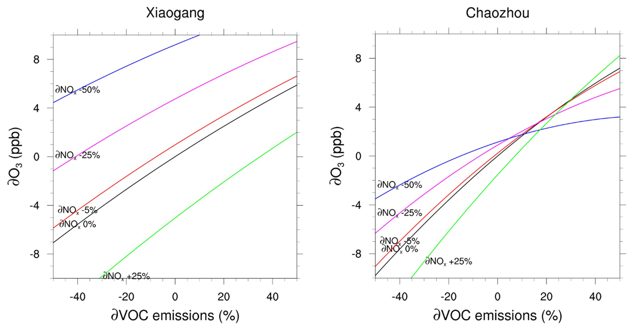
Figure 7Taylor-series approximation of ∂O3 against ∂VOC emissions at different levels of projected ∂NOx emissions for Xiaogang (urban) and Chaozhou (inland) averaged at 12:00 LST. Projected ∂NOx emissions at 0 % (black line) and −5 % (red line) represent the current year of 2018 and the near future of 2025, respectively; other projected ∂NOx emissions at arbitrary values of −50 % and ±25 % are presented for far-future comparison purposes.
3.3 Sensitivity of individual modeled VOC species
In this subsection, we further evaluate the sensitivity of the ozone response to individual modeled VOC emissions using the CMAQ direct decoupled method (DDM-3D). Note that only the first-order sensitivity coefficient of individual VOC species in CB6 is calculated, considering the high computational cost, and the second-order sensitivity coefficients of ozone to total VOC emissions have a low contribution. A total of 20 individual sensitivity tests were performed to target each modeled lumped VOC class or individual species (refer to Table 1 for a complete list of modeled VOC species). Figure 8a shows the daytime CMAQ-DDM sensitivity coefficient of ozone to the VOC emissions, arranged in ascending order and separated for the urban and inland area. The urban area sensitivity coefficients are substantially higher than that in the inland area for all species, which is expected due to the VOC-limited regime in the urban area. Among the 20 VOC species, the six most important VOC species were identified as XYL (xylene), OLE (terminal C–C olefins), PAR (paraffins), ETH (ethene), TOL (toluene), and IOL (internal C–C olefins).
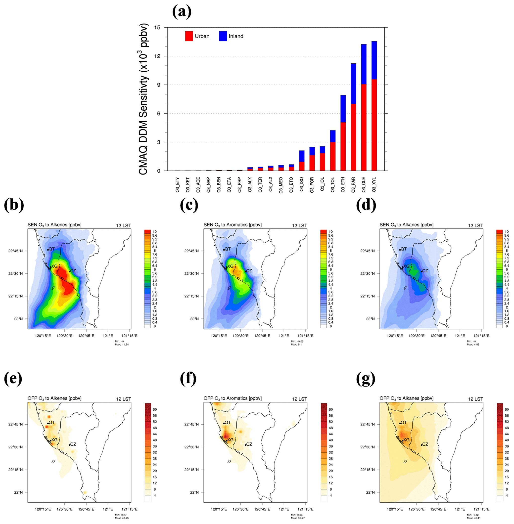
Figure 8(a) Daily averaged CMAQ-DDM first-order sensitivity coefficient of O3 concentrations calculated per number of grids for each modeled VOC species arranged in ascending order for the urban and inland area. Sensitivity of O3 and ozone formation potential (OFP) to (b, e) alkene emissions (OLE + ETH + IOL), (c, f) aromatic emissions (XYL + TOL), and (d, g) alkane emissions (PAR) at 12:00 LST.
XYL and TOL are aromatic hydrocarbons that are included in the BTEX group, along with benzene and ethylbenzene. The ranking of BTEX with respect to ozone formation potential in a high-NOx environment is often done using maximum incremental reactivity (MIR), which uses unitless coefficients and indicates the amount contributed to ozone formation in the air mass by individual compounds. Based on the MIR scale adopted from the literature (Atkinson, 1997; Carter, 1994), m-xylene and p-xylene (8.20) are the most dominant contributors to ozone formation among BTEX, followed by toluene (2.70), ethylbenzene (2.70), and benzene (0.42). Our result agrees with the MIR scale, which yielded classifications of XYL and TOL as the second and fifth most sensitive VOC species to O3 among the 20 VOC species considered in the sensitivity tests. Other sensitive VOC species to O3 formation include alkanes (i.e., PAR (MIR=0.32)) and alkenes (i.e., OLE (8.24), ETH (4.37), IOL (13.11)).
To gain additional insights about the ozone response to the six most sensitive VOC species, we grouped them into three categories (i.e., alkenes: OLE, ETH, and IOL; aromatics: TOL and XYL; and alkanes: PAR) and plotted the spatial distributions of the sensitivities at 12:00 LST (Fig. 8b–d). The sensitivity of ozone to alkenes and alkanes has a similar pattern with higher sensitivity concentrated near the emission source and slightly shifted towards inland/mountainous areas and Pingtung county due to the local circulation and the prevailing northeasterly winds. For the sensitivity of ozone to aromatics, the spatial distribution has a smaller area coverage, and higher sensitivity is more concentrated near the emission source. To render a clearer picture on the spatial distribution of O3 sensitivity for each VOCs component, the spatial distribution of some highly sensitive VOC component emissions (i.e., XYL, OLE, PAR, ETH, TOL, IOL) is provided in the Supplement (see Fig. S8). The role of land–sea-breeze circulation in transporting the local O3 precursors (i.e., VOC) from the urban to inland area is well reflected by the diurnal profile of the sensitivity coefficients (Fig. 9). An obvious shift is simulated in the inland area as compared to the urban area; the urban sensitivity coefficients peak at 10:00 LST, while the peak in the inland area is at 13:00 LST. A lag of 2–3 h is mainly attributed to the daytime sea-breeze penetration that pushes the urban polluted air towards the inland area due to the differential heating between the land and sea surfaces during the noon hours. This result also tells us that VOC emissions from the urban area are largely responsible for the inland high-ozone episodes.
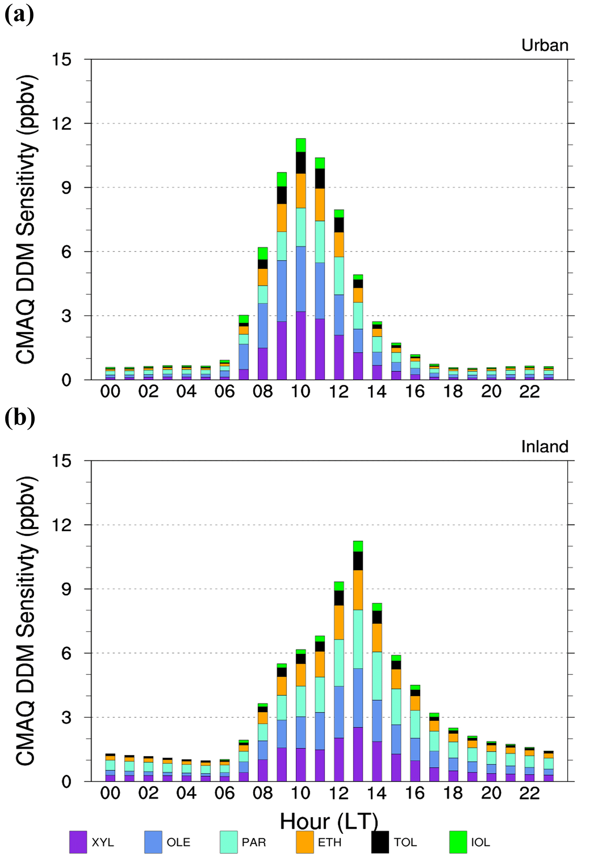
Figure 9Diurnal variations of the CMAQ-DDM sensitivity of O3 to the six most sensitive VOC modeled species (i.e., terminal olefins, OLE; xylene, XYL; paraffin, PAR; ethene, ETH; toluene; TOL; internal olefins, IOL) averaged for the (a) urban and (b) inland area, during the entire simulation period.
Using an approach similar to OFP, we quantified the relative ground-level ozone impacts of the six most sensitive VOC species by multiplying the MIR coefficients to its corresponding concentrations at 12:00 LST (see Fig. 8e–g). Due to the abundance of PAR, OFP calculated for alkane emission is significant over the western coastal region of southern Taiwan. The longer atmospheric lifetime of alkanes makes them more susceptible to transportation and impacting a wider area. Despite alkanes having the lowest sensitivity coefficient of the six groups of VOCs in the study, the significance of alkane OFP extends over a larger area, highlighting the need for controlling alkane-related emissions to reduce the ozone pollution problem over the study area. OFP of alkenes features a point source distribution pattern, indicating it is more likely related to large point source emissions. OFP of aromatics has the smallest area coverage and is highly concentrated near the populated industrial park of the study area in southern Taiwan. Among the three main contributors, aromatics have the highest maxima OFP value (56 ppbv), followed by alkenes (49 ppbv) and alkanes (40 ppbv).
Figure 10 shows the relative sensitivities for each modeled VOC to O3 (DDM – Fig. 10a) and its corresponding emission rate (EMIS – Fig. 10b) averaged in urban and inland areas during the entire simulation period. Similar to the above analysis, the three main contributors were identified as alkenes (42.2 % for urban; 37.1 % for inland), aromatics (29.1 %; 25.1 %), and alkanes (18.2 %; 23.4 %). Other less important contributors were formaldehyde (4.1 %; 3.9 %), isoprene (2.3 %; 5.4 %), alcohols (1.9 %; 2.6 %), and aldehydes (0.9 %; 1.6 %). Due to the abundant biogenic emissions surrounding the inland area, inland ozone is more sensitive to isoprene (5.4 %) as compared to the urban area. Besides, inland ozone is also more sensitive to alcohols (MEOH + ETOH) and aldehydes (ALD2 + ALDX) when compared to the urban area. This is also consistent with the higher contributions of alcohols (10.0 %) and aldehydes (1.4 %) inland than in urban areas (4.3 % and 0.8 %, respectively) (Fig. 10b).
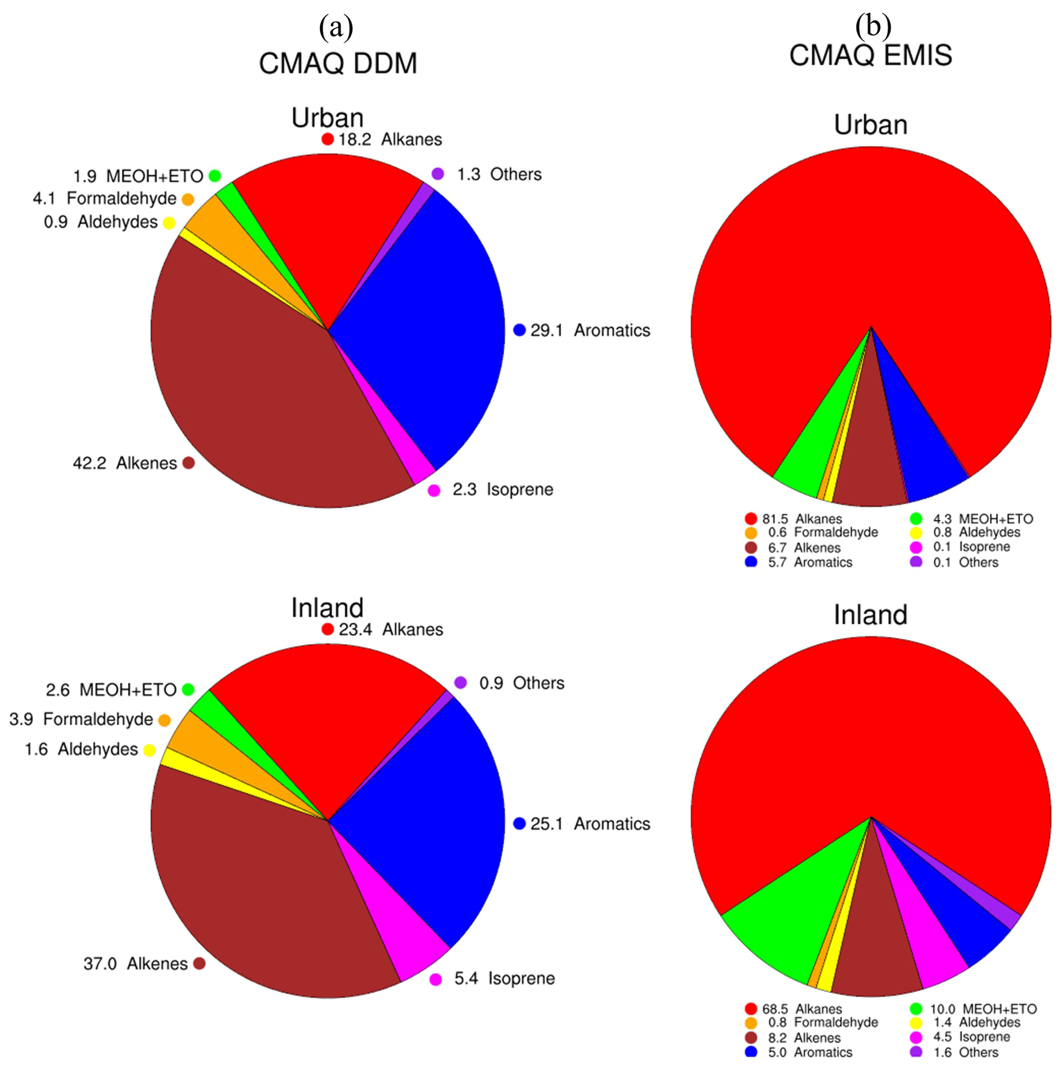
Figure 10Relative distribution in percentage of (a) CMAQ-DDM O3 sensitivity and (b) CMAQ-EMIS hydrocarbon emissions to individual VOCs summed across different groups averaged for the urban and inland area during the entire simulation period.
Overall, the DDM sensitivity tests identified three main speciated VOC groups contributing to ozone formation, namely alkenes, aromatics, and alkanes. The six most sensitive VOC surrogates in CB6 to ozone formation in the study area are XYL, OLE, PAR, ETH, TOL, and IOL in descending order. Sources of these targeted VOC species are highly variable, and previous studies have attributed these species to a wide range of emission sources not limited to traffic, industrial, petrochemical, manufacturing, solvent usage, etc. Therefore, in order to identify the sources of these VOC species for better emission control policy, source apportionment is necessary.
3.4 Descriptive statistics of PAMS-VOC data and PMF optimal solution
In this subsection, we first describe the statistics of the PAMS-VOC data measured at Chaozhou (CZ), Qiaotou (QT), and Xiaogang (XG) which were used to drive the PMF source apportionment. The CZ station is an inland station located far away from the urban core, while QT and XG are urban stations. The top 15 major VOC species measured at the three PAMS stations are summarized in Table 3, and other species are shown in Fig. S9 in the Supplement. These top 15 major VOC species accounted for 65.9 %, 70.7 %, and 68.7 % of the total VOC concentrations in CZ, QT, and XG, respectively. Overall, aromatics contributed the largest proportion, accounting for 117.3 ppbv (43.5 %) in CZ, 312.2 ppbv (53.9 %) in QT, and 361.7 ppbv (51.2 %) in XG. Toluene was the most abundant VOC species in all three stations, accounting for 46.3 ± 45.0 ppbv (17.2 % of total) in CZ, 140.4 ± 96.2 ppbv (24.3 %) in QT, and 143.0 ± 97.7 ppbv (20.2 %) in XG. Toluene is also commonly used in the chemical industry (Mo et al., 2015), the iron and steel industry (Nogueira et al., 2011), fuel evaporation (Wu et al., 2016), and organic solvent usage (Chen et al., 2019), and it is a by-product of vehicle exhaust (Dai et al., 2013). The second largest contributor to total VOC concentrations were alkanes, accounting for 42.7 % in CZ, 40.0 % in QT, and 40.6 % in XG. Among the alkanes, n-butane, propane, and isopentane comprised the highest proportions, each reaching around 5 % of the total VOC concentrations. n-Butane isomers are emitted from a variety of sources including petroleum production and natural gas emissions (Rossabi and Helmig, 2018). In the alkene category, ethylene and propylene are major contributors which are commonly used as raw materials in the petrochemical industry and refineries. Among the three stations, the highest proportion of alkene groups is observed in XG, accounting for 7.0 % of total VOC concentrations, with 3.6 % attributed to propylene.
Table 3Concentration (mean ± SD) and proportions (%) of the top 15 PAMS-VOC species in ascending order at CZ, QT, and XG during 1–31 October 2018. Bold/italic species represent the unique species that present in the top 15 at each station. All units in parts per billion (ppb).

Determining the number of factors is a critical step in receptor-based source apportionment methods like PMF analysis. Combinations of three to eight sources were used to determine the optimum number of VOC sources for each PAMS station. We also calculated the uncorrelated bootstrap (BS) mapping to assist in identifying the optimum number of factors in each station. A high number of uncorrelated BS mapping indicates excessive factors are fitted in the model; therefore, this number should be kept as low as possible to avoid over-fitting. In CZ, the was at a minimum in the six-factor solution, and the uncorrelated BS mapping was low (n=3), indicating this was the optimal solution for that site (Fig. S10 in the Supplement). Using the same protocol, the optimal solution was determined as seven factors for QT and five factors for XG. Overall, a total of eight unique factors were identified at the three stations: biogenic sources, solvent usage, vehicle emissions, plastic industry, manufacturing industry, mixed industry, aged air mass, and motorcycle exhausts (Fig. 11). The diurnal variations of the PMF factor contribution at Chaozhou, Qiaotou, and Xiaogang PAMS stations are also shown in Fig. 12. Among the eight resolved factor profiles, vehicle emissions (22 %) were the largest contribution to total VOC concentrations, followed by mixed industry (21 %), solvent usage (17 %), biogenic sources (12 %), plastic industry (10 %), and other factor profiles (i.e., aged air mass, motorcycle exhausts, and manufacturing industry). The diurnal pattern of factor distribution of the biogenic sources displays a clear diurnal cycle peak at noontime, 10:00–12:00 LST, in all three stations. Meanwhile, the motor exhaust and vehicle emission sector peak during the morning and evening traffic rush hours. The aged air mass sector is only identified in CZ, and its hourly factor contribution mostly existed at more stable levels when compared to other factors except for an obvious peak at 12:00 LST due to the sea-breeze penetration that pushes the urban polluted aged air mass towards inland area. The diurnal pattern related to industrial activity exhibits different peak hours depending on sector and station. For instance, the hourly factor contribution of solvent usage in XG has a clear bimodal peak at 10:00 and 16:00 LST, plastic industry in QT and CZ has a clear diurnal cycle peak in around noontime at 11:00 and 13:00 LST, and mixed industry in QT and XG has a clear bimodal peak at 07:00 and 18:00 LST. Details of each source profile and comparison with other PMF studies are discussed in the Supplement – “Source Profiles of PMF Model”.
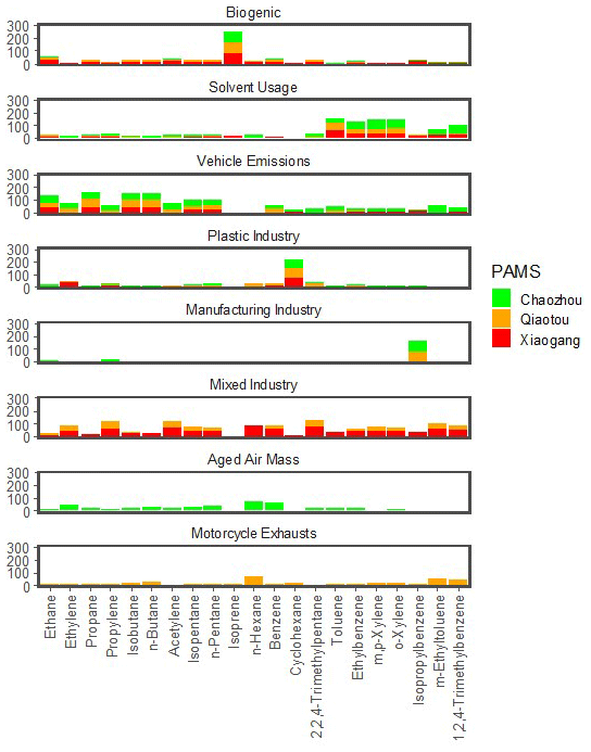
Figure 11Source profiles calculated using the PMF model at Chaozhou, Qiaotou, and Xiaogang PAMS stations.
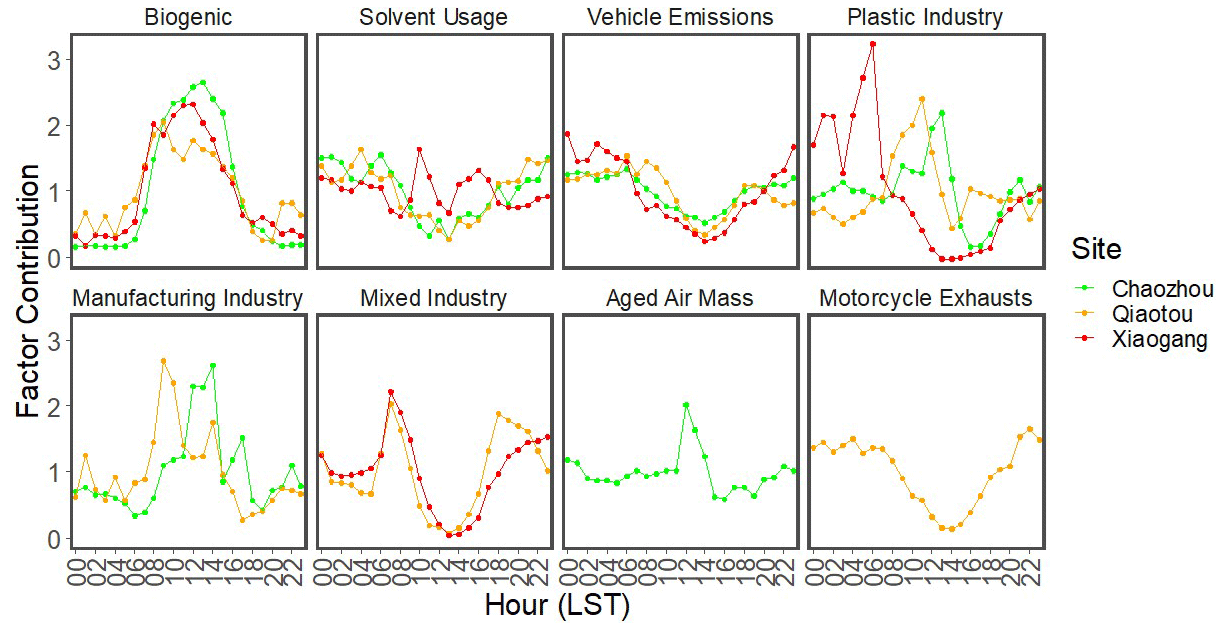
Figure 12Diurnal variations of factor contribution calculated by the PMF model at Chaozhou, Qiaotou, and Xiaogang PAMS stations.
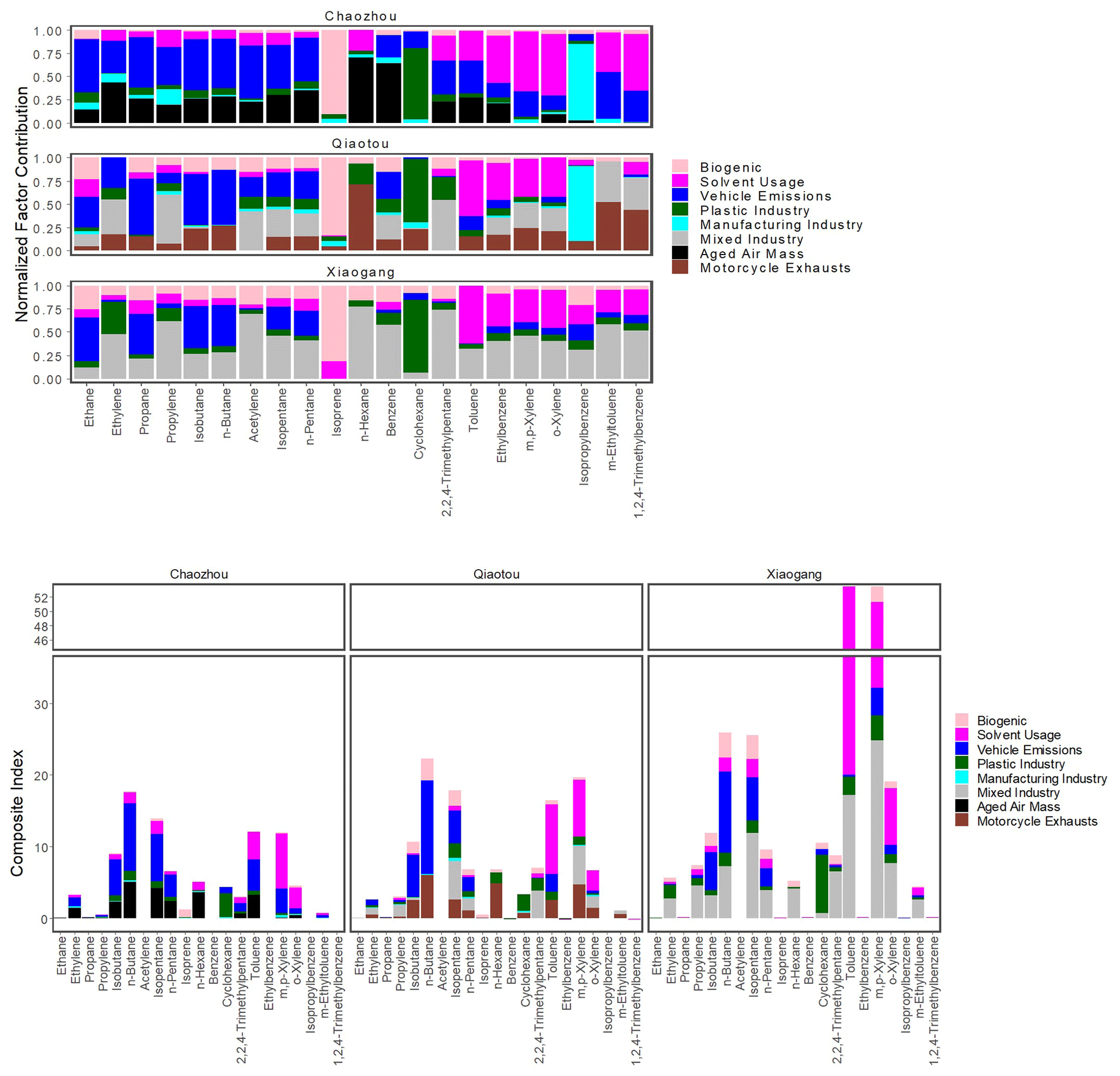
Figure 13Normalized factor contribution and composite index of source profile to each PAMS-VOC species at Chaozhou, Qiaotou, and Xiaogang PAMS station.
3.5 Dominant sources of highly sensitive VOC species
We then mapped the CMAQ-CB6-modeled VOC species to the PMF apportioned sources in order to identify the dominant sources of highly sensitive VOC species (i.e., XYL, OLE, PAR, ETH, TOL, IOL). The dominant sources of alkene species (OLE, ETH, IOL) were identified using ethylene and propylene as tracers; sources of TOL were tracked by toluene and m-ethyltoluene; sources of XYL were tracked by all three xylene isomers; and sources of PAR were identified using isobutane, n-butane, isopentane, n-pentane, n-hexane, and 2,2,4-trimethylpentane.
We also developed a composite index, ψ, to quantitatively combine the CMAQ-DDM sensitivity coefficient and PMF-resolved factor contribution in order to identify the key VOC species for an effective ozone abatement strategy. The index was calculated according to the jth species and kth source:
where C is the trace gas (O3) concentration, ε is the unitless scaling factor for the j emission (see Eqs. 2 and 3), fkj is the jth species concentration to the kth source. The first term in Eq. (9) is obtained from the CMAQ-DDM-calculated first-order sensitivity coefficient where a higher value denotes greater sensitivity (extreme low sensitivity <0.01 ppb is masked out); the second term is the PMF-resolved factor contribution where higher values of a particular species, j, indicate greater apportionment to the source, k. Higher values of the composite index indicate a greater priority should be given to that source species.
According to the PMF source apportionment (Fig. 13), the dominant source of alkene-related emissions (OLE, IOL, ETH) was attributed to mixed industry (i.e., petrochemical industry, printing industry, and metal industry) (Chen et al., 2022; Pinthong et al., 2022). This source profile contributed 61.5 % propylene and 47.6 % ethylene in XG, as well as 52.4 % propylene and 37.9 % ethylene in QT. Meanwhile, propylene and ethylene in CZ were mainly attributed to vehicle emissions and aged air masses. Given that alkene-related emissions are closely linked to large point sources (see Fig. 8e), control of alkene emissions should focus on the mixed industry, particularly petrochemical plants. Among the three stations, the highest composite index associated with ethylene and propylene summed across all factors was obtained at XG. Though ethylene and propylene have higher sensitivities compared to other species, their composite index (ψETHY, all k=5.7 and ψPROP, all k=7.4 – see Fig. 13) is relatively low due to their low abundance, 11.5 ppb (1.6 % of total VOCs) and 25.5 ppb (3.6 %), respectively, making them less important in terms of priority.
The highest composite index was assigned to aromatic compounds such as toluene (ψTOL, all k=12.1, 16.4, and 53.5 in CZ, QT, and XG, respectively), m,p-xylene (, 19.7, and 53.5), and o-xylene (ψo-XYL, all k=4.5, 6.7, and 19.0) due to their high-abundance toluene, 46.3–143.0 ppb (17.2 %–24.3 % of total VOCs), m,p-xylene, 13.6–63.8 ppb (5.0 %–9.0 %), and o-xylene, 5.2–23.3 ppb (1.9 %–3.3 %), in all three stations (see Fig. 13 and Table 3). Although toluene has much higher abundance than xylene, the composite index for both species summed across all sources is similar because the sensitivity coefficient of xylene ( ppb) is relatively higher than toluene ( ppb) (see Fig. 8a). This indicates that emission control of both of these compounds is of high priority considering their high abundance and high sensitivity in ozone formation. The dominant sources of aromatic-related emissions (XYL, TOL) are mainly attributed to solvent usage and mixed industry. Solvent usage, including building coatings, paint thinners, and other products thinners (Li et al., 2021; Chen et al., 2019; Wu et al., 2016; Huang and Hsieh, 2020), contributed 64.5 % xylene and 32.2 % toluene in CZ, 40.6 % xylene and 29.7 % toluene in QT, and 38.5 % xylene and 43.3 % toluene in XG. Mixed industry contributed 26.2 % xylene and 21.9 % toluene in QT, as well as 43.5 % xylene and 45.3 % toluene in XG. Vehicle emissions, including motorcycle exhaust, contributed less than 10 % of xylene and toluene in CZ and QT. Therefore, emission control of XYL and TOL should target solvent usage, particularly painting, coating, synthetic fragrances, adhesives and cleaning agents, and industrial sources in the region.
The dominant source of alkane-related emissions (i.e., PAR) is attributed to vehicle emissions in all three stations. The main tracers identified in the PMF source apportionment related to vehicle emissions are isobutane, n-butane, isopentane, and n-pentane; these compounds accounted for 54.9 %, 53.0 %, 47.0 %, and 47.0 % of the PMF normalized factor contribution in CZ; 54.8 %, 58.7 %, 25.9 %, and 29.1 % in QT; and 44.5 %, 43.8 %, 23.9 %, and 26.8 % in XG, respectively. Motorcycle exhaust also contributed to these compounds, but the average contribution was relatively lower (e.g., <20 % in QT). High amounts of C4–C5 alkanes (i.e., isobutane, n-butane, isopentane, n-pentane) are known indicators of traffic-related sources (S. Yu et al., 2021; Huang and Hsieh, 2020; Chen et al., 2019). Among these compounds, n-butane had the highest composite index due to its high abundance, 15–34 ppb (5.1 %–5.5 % of total VOCs). Other than freshly emitted vehicle emissions, aged air masses also contributed a significant amount (∼30 %) to these compounds at CZ, reflecting the role of land–sea-breeze circulation transporting urban vehicle plumes inland. In addition, acetylene is a well-known indicator for combustion sources and related to liquefied petroleum gas (LPG) leakage. The ratio of propane, n-butane, or i-butane to acetylene is often used to assess the domination of the LPG-vehicle sources across different cities (An et al., 2014). These ratios were 0.7, 0.8, and 0.4 in CZ; 6.0, 8.2, and 3.9 in QT; and 2.9, 3.8, and 1.7 in XG, respectively, which were much lower than 11.5, 1.8, and 2.6 in Guangzhou (Zhang et al., 2013) and 11.4, 5.0, and 2.3 in Mexico City (Blake and Rowland, 1995), which are heavily impacted by LPG-vehicle emissions. This indicates that there were relatively fewer LPG-fueled vehicles in southern Taiwan, whereas LPG is merely used to fuel a gas stove for domestic household use or catering. Therefore, emission control of PAR species should focus on the gasoline-fueled vehicle emissions, particularly in heavy-traffic cities.
In this work, we used the CMAQ-DDM-3D sensitivity tool in conjunction with PMF model source apportionment to provide a comprehensive analysis of the major contributors to VOC species and the ozone formation potential (OFP) over an area of southern Taiwan. We developed a composite index that quantitatively combines the CMAQ-DDM sensitivity coefficient and PMF-resolved factor contribution to identify the key VOC source species for the effective ozone abatement strategy, which is applicable to other urban areas that are characterized by the VOC-limited condition. A representative case in October 2018 with a daily 8 h maxima O3>75 ppb occurring often was the focus of this study. Low NOx levels and high biogenic volatile organic compound (BVOC) levels in the inland areas yielded a NOx-limited regime. Although reducing NOx emissions can reduce the inland O3 concentrations, it could adversely increase urban O3 due to the reduced titration effect. This is because the O3 sensitivity production in the urban area is mainly dominated by VOC-limited regime, and further reducing NOx emissions can suppress the titration effect and eventually increase the urban O3 concentration. In contrast, control of VOC emissions is effective in the urban area to reduce O3 concentrations and has no adverse effect in the rural area. Our DDM sensitivity analysis identified the six most sensitive VOC species or groups: XYL (xylene), OLE (terminal olefins), PAR (paraffins), ETH (ethene), TOL (toluene), and IOL (internal olefins) in descending order, which are mainly attributed to the petrochemical industry, painting and printing industry, and vehicle emissions. Based on a composite index, effective ozone abatement strategies should prioritize (1) solvent usage such as the painting, coating, and printing industry that emits abundant toluene and xylene; (2) petrol vehicular emissions with high compositions of n-butane, isopentane, isobutane, and n-pentane; and (3) the petrochemical industry with emphasis on ethylene and propylene.
Besides, our DDM results also highlighted the important role of formaldehyde in OFP over the study area given that it is ranked the seventh highest VOC species for O3 sensitivity and on a per-molecule basis for O3 sensitivity is similar to alkene (i.e., OLE, ETH, IOL) and aromatic (XYL, TOL) species. Mapping of formaldehyde to the PMF source apportionment was not done due to the lack of oxygenates in the PAMS measurement inventories. Thus, oxygenates such as FORM, ALD2, ALDX, ACET, and KET along with alcohols (ETOH and MEOH) should be included in the PMF source apportionment for more complete source identification in future studies. In the current work, WRF and CMAQ are resolved at a high resolution of 1 km to best represent the features of local circulations (i.e., land–sea breeze, urban heat island effect) at the urban scale. However, simulation at 1 km is obviously too expensive for large domain or regional modeling. The differences in HDDM and PMF analysis between D03 (3 km) and D04 (1 km) due to grid resolution remain an open question which deserves future in-depth investigations. Although the performance of the simulated meteorological parameters (T2, WS, and WD) at both urban and rural stations is acceptable in the benchmark recommended by the US EPA, notable differences in temperature (underestimation) and wind speed (overestimation) are still observable in our simulation work. These biases could be susceptible to underestimation in photochemical ozone production due to the fictitious cold bias and enhanced dispersion. Therefore, careful treatment on the urban-scale data assimilation in temperature, wind field, and relative humidity are recommended in the future to improve the model prediction.
Other important findings obtained in this study are summarized below.
-
Negative (positive) first-order sensitivities to daytime NOx emissions are dominant in the urban (inland) area, indicating ozone production sensitivity favors the VOC-limited regime (NOx-limited regime). Negative sensitivities are also extended to some parts of the coastal area of Pingtung county, reflecting the downwind transport of the urban NOx by the steering northeasterly winds due to the terrain effects and local circulations.
-
Most of the urban areas (except Xiaogang, an industrial park) exhibited negative first-order and second-order sensitivities to daytime NOx emissions, indicating a negative O3 convex response. However, due to the large negative second-order sensitivities, the urban O3 increases from the linear effect are largely attenuated by the nonlinear effect. As a result, urban O3 becomes less sensitive to changes in NOx emissions but more sensitive to VOC emissions, which favors the VOC-limited conditions.
-
Based on the PMF model source apportionment, a total of eight factor profiles are identified as mixed industry (21 %), vehicle emissions (22 %), solvent usage (17 %), biogenic sources (12 %), plastic industry (10 %), aged air mass (7 %), motorcycle exhausts (7 %), and manufacturing industry (5 %).
-
The benefit of VOC control in inland areas is expected to decrease gradually when NOx emissions continue to decrease over the long-term, but control of VOCs in highly polluted urban areas remains effective despite a large reduction in NOx in the future.
The code of the WRF software was obtained from https://doi.org/10.5065/1dfh-6p97 (Skamarock et al., 2019). The code of the CMAQ software was taken from https://github.com/USEPA/CMAQ/ (last access: 1 March 2021) and https://doi.org/10.5281/zenodo.7218076 (US EPA Office of Research and Development, 2022). The FNL data were adopted from https://doi.org/10.5065/D6M043C6 (NCEP FNL, 1999). The positive matrix factorization model for environmental data analyses was obtained from https://www.epa.gov/air-research/positive-matrix-factorization-model-environmental-data-analyses (last access: 1 March 2021; Norris et al., 2014). The observational data of surface meteorology, air pollutant, and photochemical assessment monitoring stations (PAMS) were provided by the Taiwan Environmental Protection Agency (TEPA) at https://www.epa.gov.tw (last access: 1 March 2021; Taiwan EPA, 2021).
The supplement related to this article is available online at: https://doi.org/10.5194/acp-23-6357-2023-supplement.
JHWC: conceptualization; methodology; investigation; formal analysis; validation; software; and writing – original draft. SMG: visualization; writing – reviewing and editing. SSKK: formal analysis; software. MTC: formal analysis; software. NHL: visualization; funding acquisition; writing – reviewing and editing.
The contact author has declared that none of the authors has any competing interests.
Publisher's note: Copernicus Publications remains neutral with regard to jurisdictional claims in published maps and institutional affiliations.
The authors gratefully acknowledge all assistants involved in the cluster system installation and maintenance at the Cloud and Aerosol Laboratory (CAL). The authors would like to acknowledge EPA Taiwan and CWB Taiwan for the provision of the ground-based measurement datasets as well as MODIS for satellite products and imagery.
This research has been supported by the Ministry of Science and Technology, Taiwan (grant no. MOST 111-2111-M-008-024); the Environmental Protection Administration, Taiwan; and the Elite Scholarship from the Ministry of Education, Taiwan.
This paper was edited by Joshua Fu and reviewed by two anonymous referees.
An, J., Zhu, B., Wang, H., Li, Y., Lin, X., and Yang, H.: Characteristics and source apportionment of VOCs measured in an industrial area of Nanjing, Yangtze River Delta, China, Atmos. Environ., 97, 206–214, https://doi.org/10.1016/j.atmosenv.2014.08.021, 2014.
Arter, C. A. and Arunachalam, S.: Assessing the importance of nonlinearity for aircraft emissions' impact on O3 and PM2.5, Sci. Total Environ., 777, 146121, https://doi.org/10.1016/j.scitotenv.2021.146121, 2021.
Atkinson, R.: Gas-phase tropospheric chemistry of volatile organic compounds: 1. Alkanes and alkenes, J. Phys. Chem. Ref. Data, 26, 215–290, https://doi.org/10.1063/1.556012, 1997.
Bergin, M. S., Russell, A. G., Odman, M. T., Cohan, D. S., and Chameides, W. L.: Single-source impact analysis using three-dimensional air quality models, J. Air Waste Manage., 58, 1351–1359, https://doi.org/10.3155/1047-3289.58.10.1351, 2008.
Blake, D. R. and Rowland, F. S.: Urban leakage of liquefied petroleum gas and its impact on Mexico City air quality, Science, 269, 953–956, https://doi.org/10.1126/science.269.5226.953, 1995.
Borge, R., Alexandrov, V., José del Vas, J., Lumbreras, J., and Rodríguez, E.: A comprehensive sensitivity analysis of the WRF model for air quality applications over the Iberian Peninsula, Atmos. Environ., 42, 8560–8574, https://doi.org/10.1016/j.atmosenv.2008.08.032, 2008.
Carter, W. P. L.: Development of ozone reactivity scales for volatile organic compounds, J. Air Waste Manage., 44, 881–899, https://doi.org/10.1080/1073161x.1994.10467290, 1994.
Chang, C. C., Chen, T. Y., Lin, C. Y., Yuan, C. S., and Liu, S. C.: Effects of reactive hydrocarbons on ozone formation in southern Taiwan, Atmos. Environ., 39, 2867–2878, https://doi.org/10.1016/j.atmosenv.2004.12.042, 2005.
Chang, C.-T., Wang, L., Wang, L. J., Liu, C. P., Yang, C. J., Huang, J. C., Wang, C. P., Lin, N. H., and Lin, T. C.: On the seasonality of long-range transport of acidic pollutants in East Asia, Environ. Res. Lett., 17, 094029, https://doi.org/10.1088/1748-9326/ac8b99, 2022.
Chang, J. H. W., Griffith, S. M., and Lin, N. H.: Impacts of land-surface forcing on local meteorology and ozone concentrations in a heavily industrialized coastal urban area, Urban Clim., 45, 101257, https://doi.org/10.1016/j.uclim.2022.101257, 2022.
Chen, C. H., Chuang, Y. C., Hsieh, C. C., and Lee, C. S.: VOC characteristics and source apportionment at a PAMS site near an industrial complex in central Taiwan, Atmos. Pollut. Res., 10, 1060–1074, https://doi.org/10.1016/j.apr.2019.01.014, 2019.
Chen, F. and Dudhia, J.: Coupling and advanced land surface-hydrology model with the Penn State-NCAR MM5 modeling system. Part I: Model implementation and sensitivity, Mon. Weather Rev., 129, 569–585, https://doi.org/10.1175/1520-0493(2001)129<0569:CAALSH>2.0.CO;2, 2001.
Chen, K. S., Ho, Y. T., Lai, C. H., Tsai, Y. A., and Chen, S. J.: Trends in concentration of ground-Level ozone and meteorological conditions during high ozone episodes in the Kao-Ping Airshed, Taiwan, J. Air Waste Manage., 54, 36–48, https://doi.org/10.1080/10473289.2004.10470880, 2004.
Chen, P., Zhao, X., Wang, O., Shao, M., Xiao, X., Wang, S., and Wang, Q.: Characteristics of VOCs and their potentials for O3 and SOA formation in a medium-sized city in Eastern China, Aerosol Air Qual. Res., 22, 2013–2019, https://doi.org/10.4209/aaqr.210239, 2022.
Chen, S. P., Liu, W. T., Hsieh, H. C., and Wang, J. L.: Taiwan ozone trend in response to reduced domestic precursors and perennial transboundary influence, Environ. Pollut., 289, 117883, https://doi.org/10.1016/j.envpol.2021.117883, 2021.
Cheng, F. Y., Jian, S. P., Yang, Z. M., Yen, M. C., and Tsuang, B. J.: Influence of regional climate change on meteorological characteristics and their subsequent effect on ozone dispersion in Taiwan, Atmos. Environ., 103, 66–81, https://doi.org/10.1016/j.atmosenv.2014.12.020, 2015.
Chi, X., Liu, C., Xie, Z., Fan, G., Wang, Y., He, P., Fan, S., Hong, Q., Wang, Z., Yu, X., Yue, F., Duan, J., Zhang, P., and Liu, J.: Observations of ozone vertical profiles and corresponding precursors in the low troposphere in Beijing, China, Atmos. Res., 213, 224–235, https://doi.org/10.1016/j.atmosres.2018.06.012, 2018.
Chou, M.-D. and Suarez, M. J.: A shortwave radiation parameterization for atmospheric studies, NASA Tech, 15, NASA/TM-1999-104606/VOL15, 1999.
Chuang, M. T., Chiang, P. C., Chan, C. C., Wang, C. F., Chang, E. E., and Lee, C.-T.: The effects of synoptical weather pattern and complex terrain on the formation of aerosol events in the Greater Taipei area, Sci. Total Environ., 399, 128–146, https://doi.org/10.1016/j.scitotenv.2008.01.051, 2008.
Cohan, D. S., Hakami, A., Hu, Y., and Russell, A. G.: Nonlinear response of ozone to emissions: Source apportionment and sensitivity analysis, Environ. Sci. Technol., 39, 6739–6748, https://doi.org/10.1021/es048664m, 2005.
Daellenbach, K. R., Stefenelli, G., Bozzetti, C., Vlachou, A., Fermo, P., Gonzalez, R., Piazzalunga, A., Colombi, C., Canonaco, F., Hueglin, C., Kasper-Giebl, A., Jaffrezo, J.-L., Bianchi, F., Slowik, J. G., Baltensperger, U., El-Haddad, I., and Prévôt, A. S. H.: Long-term chemical analysis and organic aerosol source apportionment at nine sites in central Europe: source identification and uncertainty assessment, Atmos. Chem. Phys., 17, 13265–13282, https://doi.org/10.5194/acp-17-13265-2017, 2017.
Dai, P., Ge, Y., Lin, Y., Su, S., and Liang, B.: Investigation on characteristics of exhaust and evaporative emissions from passenger cars fueled with gasoline/methanol blends, Fuel, 113, 10–16, https://doi.org/10.1016/j.fuel.2013.05.038, 2013.
Dunker, A. M., Yarwood, G., Ortmann, J. P., and Wilson, G. M.: Comparison of source apportionment and source sensitivity of ozone in a three-dimensional air quality model, Environ. Sci. Technol., 36, 2953–2964, https://doi.org/10.1021/es011418f, 2002a.
Dunker, A. M., Yarwood, G., Ortmann, J. P., and Wilson, G. M.: The decoupled direct method for sensitivity analysis in a three-dimensional air quality model – Implementation, accuracy, and efficiency, Environ. Sci. Technol., 36, 2965–2976, https://doi.org/10.1021/es0112691, 2002b.
Dunker, A. M., Koo, B., and Yarwood, G.: Source apportionment of the anthropogenic increment to ozone, formaldehyde, and nitrogen dioxide by the path-integral method in a 3D model, Environ. Sci. Technol., 49, 6751–6759, https://doi.org/10.1021/acs.est.5b00467, 2015.
Fan, M. Y., Zhang, Y. L., Lin, Y. C., Cao, F., Sun, Y., Qiu, Y., Xing, G., Dao, X., and Fu, P.: Specific sources of health risks induced by metallic elements in PM2.5 during the wintertime in Beijing, China, Atmos. Environ., 246, 118112, https://doi.org/10.1016/j.atmosenv.2020.118112, 2021.
Fountoukis, C., Megaritis, A. G., Skyllakou, K., Charalampidis, P. E., Pilinis, C., Denier van der Gon, H. A. C., Crippa, M., Canonaco, F., Mohr, C., Prévôt, A. S. H., Allan, J. D., Poulain, L., Petäjä, T., Tiitta, P., Carbone, S., Kiendler-Scharr, A., Nemitz, E., O'Dowd, C., Swietlicki, E., and Pandis, S. N.: Organic aerosol concentration and composition over Europe: insights from comparison of regional model predictions with aerosol mass spectrometer factor analysis, Atmos. Chem. Phys., 14, 9061–9076, https://doi.org/10.5194/acp-14-9061-2014, 2014.
Gallus, W. A. and Bresch, J. F.: Comparison of impacts of WRF dynamic core, physics package, and initial conditions on warm season rainfall forecasts, Mon. Weather Rev., 134, 2632–2641, https://doi.org/10.1175/MWR3198.1, 2006.
Guenther, A., Karl, T., Harley, P., Wiedinmyer, C., Palmer, P. I., and Geron, C.: Estimates of global terrestrial isoprene emissions using MEGAN (Model of Emissions of Gases and Aerosols from Nature), Atmos. Chem. Phys., 6, 3181–3210, https://doi.org/10.5194/acp-6-3181-2006, 2006.
Hakami, A., Harley, R. A., Milford, J. B., Odman, M. T., and Russell, A. G.: Regional, three-dimensional assessment of the ozone formation potential of organic compounds, Atmos. Environ., 38, 121–134, https://doi.org/10.1016/j.atmosenv.2003.09.049, 2004a.
Hakami, A., Odman, M. T., and Russell, A. G.: Nonlinearity in atmospheric response: A direct sensitivity analysis approach, J. Geophys. Res.-Atmos., 109, 1–12, https://doi.org/10.1029/2003JD004502, 2004b.
Hakami, A., Seinfeld, J. H., Chai, T., Tang, Y., Carmichael, G. R., and Sandu, A.: Adjoint sensitivity analysis of ozone nonattainment over the continental United States, Environ. Sci. Technol., 40, 3855–3864, https://doi.org/10.1021/es052135g, 2006.
Hsu, C. H. and Cheng, F. Y.: Synoptic weather patterns and associated air pollution in Taiwan, Aerosol Air Qual. Res., 19, 1139–1151, https://doi.org/10.4209/aaqr.2018.09.0348, 2019.
Huang, Y. S. and Hsieh, C. C.: VOC characteristics and sources at nine photochemical assessment monitoring stations in western Taiwan, Atmos. Environ., 240, 117741, https://doi.org/10.1016/j.atmosenv.2020.117741, 2020.
Ji, X., Xu, K., Liao, D., Chen, G., Liu, T., Hong, Y., Dong, S., Choi, S. D., and Chen, J.: Spatial-temporal Characteristics and Source Apportionment of Ambient VOCs in Southeast Mountain Area of China, Aerosol Air Qual. Res., 22, 1–15, https://doi.org/10.4209/aaqr.220016, 2022.
Koplitz, S., Simon, H., Henderson, B., Liljegren, J., Tonnesen, G., Whitehill, A., and Wells, B.: Changes in ozone chemical sensitivity in the United States from 2007 to 2016, ACS Environmental, 2, 206–222, https://doi.org/10.1021/acsenvironau.1c00029, 2021.
Kusaka, H. and Kimura, F.: Coupling a single-layer urban canopy model with a simple atmospheric model: Impact on urban heat island simulation for an idealized case, J. Meteorol. Soc. Jpn., 82, 67–80, https://doi.org/10.2151/jmsj.82.67, 2004.
Kusaka, H., Hiroaki, K., Kikegawa, Y., and Kimura, F.: A simple single-layer urban canopy model for atmospheric models: Comparison with multi-layer and slab models, Bound.-Lay. Meteorol., 101, 329–358, 2001.
Kwok, R. H. F., Baker, K. R., Napelenok, S. L., and Tonnesen, G. S.: Photochemical grid model implementation and application of VOC, NOx, and O3 source apportionment, Geosci. Model Dev., 8, 99–114, https://doi.org/10.5194/gmd-8-99-2015, 2015.
Laughner, J. and Cohen, R. C.: Direct observation of changing NOx lifetime in North American cities, Science, 366, 723–727, 2019.
Lee, Y. C., Wenig, M., and Yang, X.: The emergence of urban ozone episodes in autumn and air temperature rise in Hong Kong, Air Qual. Atmos. Hlth., 2, 111–121, https://doi.org/10.1007/s11869-009-0038-y, 2009.
Lei, W., de Foy, B., Zavala, M., Volkamer, R., and Molina, L. T.: Characterizing ozone production in the Mexico City Metropolitan Area: a case study using a chemical transport model, Atmos. Chem. Phys., 7, 1347–1366, https://doi.org/10.5194/acp-7-1347-2007, 2007.
Li, J., Yu, S., Chen, X., Zhang, Y., Li, M., Li, Z., Song, Z., Liu, W., Li, P., Xie, M., and Xing, J.: Evaluation of the WRF-CMAQ Model Performances on Air Quality in China with the Impacts of the Observation Nudging on Meteorology, Aerosol Air Qual. Res., 22, 220023, https://doi.org/10.4209/aaqr.220023, 2022.
Li, Y., Lau, A. K. H., Fung, J. C. H., Ma, H., and Tse, Y.: Systematic evaluation of ozone control policies using an Ozone Source Apportionment method, Atmos. Environ., 76, 136–146, https://doi.org/10.1016/j.atmosenv.2013.02.033, 2013a.
Li, Y., Lau, A. K. H., Fung, J. C. H., Zheng, J., and Liu, S.: Importance of NOx control for peak ozone reduction in the Pearl River Delta region, J. Geophys. Res.-Atmos., 118, 9428–9443, https://doi.org/10.1002/jgrd.50659, 2013b.
Li, Z., Li, W., Zhou, R., Miao, X., Lu, J., Wang, Z., Yang, Z., and Wu, J.: Process-based VOCs source profiles and contributions to ozone formation in typical organic solvent-used industries in Hangzhou, Aerosol Air Qual. Res., 21, 210008, https://doi.org/10.4209/aaqr.210008, 2021.
Lin, C. Y., Liu, S. C., Chou, C. C. K., Liu, T. H., Lee, C.-T., Yuan, C. S., Shiu, C. J., and Young, C. Y.: Long-range transport of Asian dust and air pollutants to Taiwan, Terr. Atmos. Ocean. Sci., 15, 759–784, https://doi.org/10.3319/TAO.2004.15.5.759(ADSE), 2004.
Lin, C. Y., Liu, S. C., Chou, C. C. K., Huang, S. J., Liu, C. M., Kuo, C. H., and Young, C. Y.: Long-range transport of aerosols and their impact on the air quality of Taiwan, Atmos. Environ., 39, 6066–6076, https://doi.org/10.1016/j.atmosenv.2005.06.046, 2005.
Ling, Z. H. and Guo, H.: Contribution of VOC sources to photochemical ozone formation and its control policy implication in Hong Kong, Environ. Sci. Policy, 38, 180–191, https://doi.org/10.1016/j.envsci.2013.12.004, 2014.
Liu, X., Wang, N., Lyu, X., Zeren, Y., Jiang, F., Wang, X., Zou, S., Ling, Z., and Guo, H.: Photochemistry of ozone pollution in autumn in Pearl River Estuary, South China, Sci. Total Environ., 754, 141812, https://doi.org/10.1016/j.scitotenv.2020.141812, 2021.
Liu, Y., Shao, M., Fu, L., Lu, S., Zeng, L., and Tang, D.: Source profiles of volatile organic compounds (VOCs) measured in China: Part I, Atmos. Environ., 42, 6247–6260, https://doi.org/10.1016/j.atmosenv.2008.01.070, 2008.
Luecken, D. J., Napelenok, S. L., Strum, M., Scheffe, R., and Phillips, S.: Sensitivity of ambient atmospheric formaldehyde and ozone to precursor species and source types across the United States, Environ. Sci. Technol., 52, 4668–4675, https://doi.org/10.1021/acs.est.7b05509, 2018.
Luecken, D. J., Yarwood, G., and Hutzell, W. T.: Multipollutant modeling of ozone, reactive nitrogen and HAPs across the continental US with CMAQ-CB6, Atmos. Environ., 201, 62–72, https://doi.org/10.1016/j.atmosenv.2018.11.060, 2019.
Mazzuca, G. M., Ren, X., Loughner, C. P., Estes, M., Crawford, J. H., Pickering, K. E., Weinheimer, A. J., and Dickerson, R. R.: Ozone production and its sensitivity to NOx and VOCs: results from the DISCOVER-AQ field experiment, Houston 2013, Atmos. Chem. Phys., 16, 14463–14474, https://doi.org/10.5194/acp-16-14463-2016, 2016.
Mo, Z., Shao, M., Lu, S., Qu, H., Zhou, M., Sun, J., and Gou, B.: Process-specific emission characteristics of volatile organic compounds (VOCs) from petrochemical facilities in the Yangtze River Delta, China, Sci. Total Environ., 533, 422–431, https://doi.org/10.1016/j.scitotenv.2015.06.089, 2015.
NCEP FNL: Operational Model Global Tropospheric Analyses, continuing from July 1999, Research Data Archive at the National Center for Atmospheric Research, Computational and Information Systems Laboratory [data set], https://doi.org/10.5065/D6M043C6 (last access: 1 March 2021), 1999.
Nogueira, F. G. E., Lopes, J. H., Silva, A. C., Lago, R. M., Fabris, J. D., and Oliveira, L. C. A.: Catalysts based on clay and iron oxide for oxidation of toluene, Appl. Clay Sci., 51, 385–389, https://doi.org/10.1016/j.clay.2010.12.007, 2011.
Norris, G., Duvall, R., Brown, S., and Bai, S.: EPA Positive Matrix Factorization (PMF) 5.0. Fundamentals and User Guide. U.S. Environmental Protection Agency, Washington, D.C., EPA/600/R-14/108 (NTIS PB2015-105147) (last access: 1 March 2021), 2014.
Pallavi, Sinha, B., and Sinha, V.: Source apportionment of volatile organic compounds in the northwest Indo-Gangetic Plain using a positive matrix factorization model, Atmos. Chem. Phys., 19, 15467–15482, https://doi.org/10.5194/acp-19-15467-2019, 2019.
Pinthong, N., Thepanondh, S., and Kondo, A.: Source identification of VOCs and their environmental health risk in a petrochemical industrial area, Aerosol Air Qual. Res., 22, 1–18, https://doi.org/10.4209/aaqr.210064, 2022.
Pleim, J. E.: A combined local and nonlocal closure model for the atmospheric boundary layer. Part I: Model description and testing, J. Appl. Meteorol. Clim., 46, 1383–1395, https://doi.org/10.1175/JAM2539.1, 2007.
Rajput, P., Mandaria, A., Kachawa, L., Singh, D. K., Singh, A. K., and Gupta, T.: Chemical characterisation and source apportionment of PM1 during massive loading at an urban location in Indo-Gangetic Plain: Impact of local sources and long-range transport, Tellus B, 68, 30659, https://doi.org/10.3402/tellusb.v68.30659, 2016.
Reff, A., Eberly, S. I., and Bhave, P. V.: Receptor modeling of ambient particulate matter data using positive matrix factorization: Review of existing methods, J. Air Waste Manage., 57, 146–154, https://doi.org/10.1080/10473289.2007.10465319, 2007.
Rossabi, S. and Helmig, D.: Changes in atmospheric butanes and pentanes and their isomeric ratios in the Continental United States, J. Geophys. Res.-Atmos., 123, 3772–3790, https://doi.org/10.1002/2017JD027709, 2018.
Sillman, S.: The relation between ozone, NOx and hydrocarbons in urban and polluted rural environments, Atmos. Environ., 33, 1821–1845, https://doi.org/10.1016/S1474-8177(02)80015-8, 1999.
Skamarock, W. C., Klemp, J. B., Dudhia, J., Gill, D. O., Liu, Z., Berner, J., Wang, W., Powers, J. G., Duda, M. G., Barker, D. M., and Huang, X.-Y.: A Description of the Advanced Research WRF Version 4, NCAR Tech. Note NCAR/TN-556+STR [data set], 145 pp., https://doi.org/10.5065/1dfh-6p97 (last access: 1 March 2021), 2019.
Taiwan EPA (Environmental Protection Agency): Taiwan EPA [data set], https://www.epa.gov.tw (last access: 1 March 2021), 2021.
Tao, W. K., Lang, S., Zeng, X., Li, X., Matsui, T., Mohr, K., Posselt, D., Chem, J., Peters-Lidard, C., Norris, P. M., Kang, I. S., Choi, I., Hou, A., Lau, K. M., and Yang, Y. M.: The Goddard Cumulus Ensemble model (GCE): Improvements and applications for studying precipitation processes, Atmos. Res., 143, 392–424, https://doi.org/10.1016/j.atmosres.2014.03.005, 2014.
Tsai, D. H., Wang, J. L., Wang, C. H., and Chan, C. C.: A study of ground-level ozone pollution, ozone precursors and subtropical meteorological conditions in central Taiwan, J. Environ. Monitor., 10, 109–118, https://doi.org/10.1039/b714479b, 2008.
US EPA Office of Research and Development: CMAQ (5.4), Zenodo [code], https://doi.org/10.5281/zenodo.7218076, 2022.
Wang, X., Li, J., Zhang, Y., Xie, S., and Tang, X.: Ozone source attribution during a severe photochemical smog episode in Beijing, China, Sci. China Chem., 52, 1270–1280, https://doi.org/10.1007/s11426-009-0137-5, 2009.
Wang, X., Fu, T. M., Zhang, L., Cao, H., Zhang, Q., Ma, H., Shen, L., Evans, M. J., Ivatt, P. D., Lu, X., Chen, Y., Zhang, L., Feng, X., Yang, X., Zhu, L., and Henze, D. K.: Sensitivities of ozone air pollution in the Beijing-Tianjin-Hebei area to local and upwind precursor emissions using adjoint modeling, Environ. Sci. Technol., 55, 5752–5762, https://doi.org/10.1021/acs.est.1c00131, 2021.
Wu, F., Yu, Y., Sun, J., Zhang, J., Wang, J., Tang, G., and Wang, Y.: Characteristics, source apportionment and reactivity of ambient volatile organic compounds at Dinghu Mountain in Guangdong Province, China, Sci. Total Environ., 548–549, 347–359, https://doi.org/10.1016/j.scitotenv.2015.11.069, 2016.
Wu, P. C. and Huang, K. F.: Tracing local sources and long-range transport of PM10 in central Taiwan by using chemical characteristics and Pb isotope ratios, Sci. Rep.-UK, 11, 7593, https://doi.org/10.1038/s41598-021-87051-y, 2021.
Xiao, X., Cohan, D. S., Byun, D. W., and Ngan, F.: Highly nonlinear ozone formation in the Houston region and implications for emission controls, J. Geophys. Res.-Atmos., 115, 1–12, https://doi.org/10.1029/2010JD014435, 2010.
Xing, J., Wang, S. X., Jang, C., Zhu, Y., and Hao, J. M.: Nonlinear response of ozone to precursor emission changes in China: a modeling study using response surface methodology, Atmos. Chem. Phys., 11, 5027–5044, https://doi.org/10.5194/acp-11-5027-2011, 2011.
Yang, Y. J., Wilkinson, J. G., and Russell, A. G.: Fast, direct sensitivity analysis of multidimensional photochemical models, Environ. Sci. Technol., 31, 2859–2868, https://doi.org/10.1021/es970117w, 1997.
Yarwood, G., Whitten, G. Z., and Jung, J.: Development, Evaluation and Testing of Version 6 of the Carbon Bond Chemical Mechanism (CB6), in: 9th Annual CMAS Conference, Chapel Hill, NC, 11–13, October 2010.
Yen, M.-C. and Chen, T.-C.: Seasonal variation of the rainfall over Taiwan, Int. J. Climatol., 20, 803–809, https://doi.org/10.1016/0032-5910(72)80020-2, 2000.
Yu, R., Lin, Y., Zou, J., Dan, Y., and Cheng, C.: Review on atmospheric ozone pollution in china: Formation, spatiotemporal distribution, precursors and affecting factors, Atmosphere-Basel, 12, 1675, https://doi.org/10.3390/atmos12121675, 2021.
Yu, S., Su, F., Yin, S., Wang, S., Xu, R., He, B., Fan, X., Yuan, M., and Zhang, R.: Characterization of ambient volatile organic compounds, source apportionment, and the ozone–NOx–VOC sensitivities in a heavily polluted megacity of central China: effect of sporting events and emission reductions, Atmos. Chem. Phys., 21, 15239–15257, https://doi.org/10.5194/acp-21-15239-2021, 2021.
Zhang, Y., Wen, X.-Y., Wang, K., Vijayaraghavan, K., and Jacobson, M. Z.: Probing into regional O3 and particulate matter pollution in the United States: 2. An examination of formation mechanisms through a process analysis technique and sensitivity study, J. Geophys. Res., 114, 1–31, https://doi.org/10.1029/2009jd011900, 2009.
Zhang, Y., Wang, X., Barletta, B., Simpson, I. J., Blake, D. R., Fu, X., Zhang, Z., He, Q., Liu, T., Zhao, X., and Ding, X.: Source attributions of hazardous aromatic hydrocarbons in urban, suburban and rural areas in the Pearl River Delta (PRD) region, J. Hazard. Mater., 250–251, 403–411, https://doi.org/10.1016/j.jhazmat.2013.02.023, 2013.
Zhao, Q., Bi, J., Liu, Q., Ling, Z., Shen, G., Chen, F., Qiao, Y., Li, C., and Ma, Z.: Sources of volatile organic compounds and policy implications for regional ozone pollution control in an urban location of Nanjing, East China, Atmos. Chem. Phys., 20, 3905–3919, https://doi.org/10.5194/acp-20-3905-2020, 2020.
Zheng, J., Zhang, L., Che, W., Zheng, Z., and Yin, S.: A highly resolved temporal and spatial air pollutant emission inventory for the Pearl River Delta region, China and its uncertainty assessment, Atmos. Environ., 43, 5112–5122, https://doi.org/10.1016/j.atmosenv.2009.04.060, 2009.