Influence of cloud microphysics schemes on weather model predictions of heavy precipitation

Cloud microphysics is one of the major sources of uncertainty in numerical weather prediction models. In this work, the ability of a numerical weather prediction model to correctly predict high-impact weather events, i.e., hail and heavy rain, using different cloud microphysics schemes is evaluated statistically. Polarimetric C-band radar observations over 30 convection days are used as the observation dataset. Simulations are made using the regional-scale Weather Research and Forecasting (WRF) model with five microphysics schemes of varying complexity (double moment, spectral bin (SBM), and Predicted Particle Properties (P3)). Statistical characteristics of heavy-rain and hail events of varying intensities are compared between simulations and observations. All simulations, regardless of the microphysics scheme, predict heavy-rain events (15, 25, and 40 mm h⁻¹) that cover larger average areas than those observed by radar. The frequency of these heavy-rain events is similar to radar-measured heavy-rain events but still scatters by a factor of 2 around the observations, depending on the microphysics scheme. The model is generally unable to simulate extreme hail events with reflectivity thresholds of 55 dBZ and higher, although they have been observed by radar during the evaluation period. For slightly weaker hail/graupel events, only the P3 scheme is able to reproduce the observed statistics. Analysis of the raindrop size distribution in combination with the model mixing ratio shows that the P3, Thompson two-moment (2-mom), and Thompson aerosol-aware schemes produce large raindrops too frequently, and the SBM scheme misses large rain and graupel particles. More complex schemes do not necessarily lead to better results in the prediction of heavy precipitation.

1 Introduction

High-impact weather events, e.g., heavy rain or hail, can lead to massive economic losses and threaten lives and livelihoods. The severe flood event in July 2021 in western Germany and neighboring countries, for example, resulted in the death of at least 170 people and insured losses of more than EUR 10 billion in Germany alone (Junghänel et al., 2021; CEDIM Forensic Disaster Analysis (FDA) Group et al., 2021). To prepare the population and infrastructure and thereby reduce these losses, national weather services typically use numerical weather prediction (NWP) models to forecast such extreme events with lead times of several days. At the German Weather Service (DWD) the ICON (Zängl et al., 2014) model is used for this purpose. However, the accuracy of NWP forecasts is limited, and some hazardous weather events, such as small-scale convective events, are difficult to predict in terms of correct location, timing, or magnitude. For example, in Belgium, operational forecast models were unable to predict a thunderstorm that produced a strong downburst less than 100 m in diameter and caused five fatalities (De Meutter et al., 2015). There is potential for improvement in several respects: increasing the resolution (e.g., Clark et al., 2016; Morrison et al., 2015) allows more and more processes to be simulated explicitly and effectively eliminates some problems caused by inaccurate parameterizations. Another aspect with potential for improvement in NWP models is the treatment of cloud microphysics (e.g., Morrison et al., 2015; Rajeevan et al., 2010), which will be the focus of this study. Microphysical processes occur on very small scales and are typically parameterized. Modelling these processes is challenging and subject to large uncertainties (Morrison et al., 2020; Fan et al., 2017). A variety of different microphysics schemes are used in current operational NWP models, varying greatly in their complexity. Typically, these schemes are categorized as either “bulk” or “bin” schemes, although other categories exist too. Briefly, bulk schemes usually predict one or more moments of a predefined statistical function representing the droplet size spectrum, while bin schemes predict mass and number concentrations for a range of sizes (bins) without imposing a particular size distribution. A good overview of the differences, advantages, and disadvantages of bulk and bin schemes can be found in Khain et al. (2015). Depending on the choice of microphysics scheme, simulation results and required computational power can vary greatly. Very simple microphysics schemes (e.g., Kessler, 1969) are cheap but also do not capture the complexity of real microphysical processes. As the complexity of the microphysics scheme increases, so does the computational power required, which is often the limiting resource in weather prediction. Therefore, an important question to answer is how much complexity in microphysics schemes is required for numerical weather prediction? Microphysics schemes often make very simple assumptions; e.g., some hydrometeors are usually simply assumed to be spherical. In part, this is due to a lack of knowledge: it is known that many processes, especially those involving ice microphysics, are poorly represented in numerical weather prediction models (Morrison et al., 2020). One reason is that direct observation of microphysical processes is very difficult due to the size of the particles involved at millimeter scales and below, as well as the many different shapes, sizes, or phases of the hydrometeors involved. Therefore, in order to constrain the processes implemented in an NWP model, observations are needed that provide such information. Direct (in situ) measurements in clouds, for example with aircraft, provide this information, but such measurements are expensive and require much effort. Moreover, it is not possible to cover several parts of the cloud or several clouds at the same time; in situ measurements are spatially limited. Radar observations, in contrast, provide measurements over a large atmospheric volume with high temporal and spatial resolution. However, the processes are not measured directly but inferred from the measured reflectivity. This is associated with numerous uncertainties, e.g., due to beam broadening effects, non-uniform beam filling, attenuation along the beam path, or variation in the refractive index due to different particle phases (e.g., hail or rain) in the same measurement volume. In addition, the reflectivity strongly depends on the particle size distribution: larger particles usually dominate the reflectance signal, since the (Rayleigh) back scattering (or radar cross-section) is proportional to the sixth power of the droplet diameter (Bringi and Chandrasekar, 2001).

In recent years, polarimetric radar measurements have become available. In 2009, DWD began upgrading the national radar network to full dual-polarimetric radars that perform operational polarimetric volume scans over all of Germany with a temporal resolution of 5 min (Helmert et al., 2014). This data are highly useful because the polarimetric information is affected by many particle population properties, such as particle phase, density, orientation, shape, size, and number concentration, and thus can be used to evaluate and improve NWP models (Ryzhkov et al., 2020). Such a dataset provides striking opportunities to evaluate properties and abilities of cloud microphysics schemes in NWP models which were previously inaccessible. In principle, NWP model output can be compared to polarimetric radar signals in two different ways: (1) converting the model output to polarimetric radar signatures using a polarimetric radar forward operator (e.g., Ryzhkov et al., 2011; Augros et al., 2015; Snyder et al., 2017) or (2) retrieving microphysical information from the polarimetric radar signal (e.g., Cao et al., 2010). These two approaches and related literature are described in a review paper by Ryzhkov et al. (2020). Polarimetric information can be used for many different applications, such as improved quantitative precipitation estimation (QPE) from radar measurements (Ryzhkov et al., 2022), hydrometeor identification (HID) algorithms (e.g., Park et al., 2009), or microphysical ice retrievals (e.g., Tetoni et al., 2022). The focus of this study is on using polarimetric radar signals to evaluate cloud microphysics schemes of an NWP model. For this assessment, we use both of the aforementioned approaches: (1) by applying a radar forward operator, we generate simulated polarimetric radar signals, and (2) by applying a hydrometeor classification, we obtain dominant hydrometeor classes from the observed radar signals, which we then compare to the simulated hydrometeors.

There are numerous publications that evaluate weather model predictions and microphysics schemes for specific events of interest that were particularly hazardous, well observed, or both (e.g., Shrestha et al., 2022; Taufour et al., 2018). This is an important approach to understand the behavior of a model in specific scenarios. However, atmospheric conditions are highly variable, and a model may perform very well in a particular situation but may provide very poor predictions under different atmospheric conditions. Statistical analysis of weather forecasts over a longer time period and across multiple weather events provides a more robust assessment of model performance but requires a large amount of effort because a large number of weather simulations and observations must be performed and checked for quality. Depending on the grid spacing and type of model used, the available computational power may also simply be insufficient to provide weather simulations in a limited amount of time. In a recent study by Köcher et al. (2022), microphysics schemes were statistically evaluated over a dataset of 30 convection days in 2019 and 2020. This dataset consists of weather simulations with five different microphysics schemes of varying complexity, as well as simultaneous polarimetric C-band radar observations from DWD, and is therefore well suited to address the aforementioned following problems:

1. How can polarimetric radar observations be used to statistically evaluate microphysics schemes?

2. What complexity of microphysics schemes is required for NWP predictions?

In Köcher et al. (2022), cloud microphysics schemes of varying complexity are assessed by a statistical comparison of the observed radar signals with the simulated radar signals from the model output. This study builds on the study of Köcher et al. (2022) and goes one step further by additionally retrieving hydrometeor information from the polarimetric radar observations and comparing it with the simulated hydrometeors. The focus is on high-impact weather events, i.e., hail and heavy rain. The goal is to exploit the potential of polarimetric radar data for an evaluation of cloud microphysics schemes to statistically describe and discuss the uncertainties of cloud microphysics in numerical weather prediction with respect to high-impact weather events.

The paper is structured as follows: Sect. 2 describes the measurement and simulation data. In Sect. 3, a model prediction is presented using a convective case as an example to show that the model is fundamentally capable of producing realistic predictions. Sections 4 and 5 then statistically evaluate the microphysics schemes using heavy-rain and hail/graupel events, respectively. Finally, Sect. 6 summarizes the results, draws conclusions, and discusses possible next steps.

2 Data and methodology

2.1 Evaluation periods

A total of 30 convective weather days in 2019 and 2020 were used for comparison. A detailed description of the radar observation and model simulation dataset can be found in Köcher et al. (2022). It is also summarized below.

The observational data are provided by the C-band radar in Isen, southern Germany, near city of Munich, which is operated by the DWD. The radar is fully dual polarimetric; therefore, polarimetric quantities such as horizontal reflectivity (Z_h), differential reflectivity (Z_dr), specific differential phase (K_dp), and cross-correlation coefficient (ρ_hv) are available. As part of the operational national radar network, the observation strategy is fixed: with a repetition rate of 5 min, a volume scan is performed, consisting of 11 plan position indicator (PPI) scans at elevation angles from 0.5 to 25^∘ over the entire 360^∘ azimuth. More information on the measurement strategy can be found in Helmert et al. (2014). This is the same dataset used in Köcher et al. (2022, referred to as “Strategy A”). Further radar characteristics of the Isen radar and the exact days of measurement are listed in Tables 1 and A1, therein. The Weather Research and Forecasting model (WRF; Skamarock et al., 2019, version 4.2) employing five different microphysics schemes of different complexity (Table 1) is used for the model simulations. The inner Munich domain has a grid spacing of 400 m and covers 144 km × 144 km. Only the inner third is used for analysis to exclude possible boundary issues.

Thompson et al. (2008)Morrison et al. (2009)Thompson and Eidhammer (2014)Shpund et al. (2019)Morrison and Milbrandt (2015)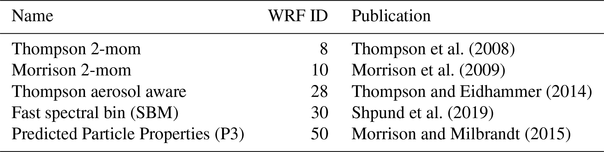

Table 1 The employed microphysics schemes.

A radar forward operator (CR-SIM; Oue et al., 2020), consistent with the corresponding microphysics scheme, is applied to the model output to simulate the same polarimetric radar signals as observed: Z_h, Z_dr, K_dp, and ρ_hv. Key assumptions of CR-SIM include particle shapes and particle orientations: cloud droplets are assumed to be spherical, and raindrops and graupel are assumed to be oblate spheroids with aspect ratios that depend on droplet size according to Brandes et al. (2002) and Ryzhkov et al. (2011), respectively. Snow and cloud ice are assumed to be oblate with fixed aspect ratios of 0.6 and 0.2, respectively. P3 deviates from the traditional schemes regarding ice and uses different ice types distributed across the particle size distribution (see Fig. 1 in Morrison and Milbrandt, 2015). Here, CR-SIM assumes that small ice and graupel are spherical, while unrimed and partially rimed ice are assumed to be oblate with an aspect ratio of 0.6. In terms of particle orientation, CR-SIM assumes that all particles are 2D Gaussian distributed with a 0^∘ mean canting angle according to Ryzhkov et al. (2011). The width of the angle distributions varies depending on the hydrometeor class: 10^∘ for clouds, rain, and ice and 40^∘ for snow, unrimed ice, partially rimed ice, and graupel. In terms of particle densities and particle size distributions, CR-SIM is consistent with the applied microphysics schemes. In most of the applied schemes, the particle density is constant and varies only between hydrometeor classes. Only the P3 scheme deviates from this, where the particle density of ice is not constant, but several mass–size relations are used. Following the P3 scheme, CR-SIM also uses multiple mass–size relations. In terms of particle size distributions, CR-SIM follows the same gamma distributions as the bulk microphysics schemes. For the SBM simulation, CR-SIM requires an additional input file containing the actual bins as simulated by the SBM scheme. There is no melting scheme applied by CR-SIM, and as a result radar signatures resulting from mixed-phased particles, such as for example a “bright band” (Austin and Bemis, 1950), cannot be simulated by the model. Further details and a discussion of the assumptions of the CR-SIM radar forward operator can be found in Köcher et al. (2022, Sect. 2.4). Attenuation effects are simulated by the radar forward operator and applied to the simulated (differential) reflectivity to obtain attenuated (differential) reflectivities from the model output.

The horizontal model grid spacing is 400 m. The DWD radar data are provided with bins every 250 m along the range axis and every 1^∘ along the azimuth. The beamwidth is about 265 m at the closer domain edge, about 685 m at the domain center, and about 1100 m at the far edge. Simulated and measured radar signals are converted to a regular Cartesian grid with a grid spacing of 400 m using inverse range interpolation. This interpolation includes the four nearest data points, weighted by their distance $(\mathrm{1}/\mathrm{distance}{)}^{\mathrm{2}}$. Both the radar and model require a sufficient spatial sampling to observe a physical phenomenon like a strong precipitation cell. Here, this translates into the question of an effective resolution, which is coarser than the nominal resolution. Skamarock (2004) estimates the effective resolution of WRF to be 5–7 times the nominal resolution, which would result in around a 2 km effective model resolution in our case. Given that a radar with a nominal sampling of around 700 m (at the domain center) also needs at least two to three samples of a precipitation cell to begin resolving its true intensity, the effective resolution of such observations seems to be in a comparable range.

2.2 Hydrometeor classification

Polarimetric radar signals can provide information on the type of hydrometeors present in the measurement volume. There are hydrometeor identification (HID) algorithms that use polarimetric radar signals to determine the dominant hydrometeor species. In this study, the algorithm of Dolan et al. (2013) for C-band radar is applied for this purpose. This algorithm uses a fuzzy logic approach (Zadeh, 1965) based on theoretical scattering simulations using the T-matrix (Barber and Yeh, 1975) and Mueller-matrix (Vivekanandan et al., 1991) models from Dolan and Rutledge (2009), originally for X-band. Based on the polarimetric radar variable ranges derived from the T-matrix scattering simulations, the method defines fuzzy logic membership functions for each hydrometeor type. These functions are then used to calculate a score describing how well the input radar signals match a hydrometeor type. There are 10 different categories available. Drizzle and rain are combined into a common class, hereafter referred to as rain. Of all the ice classes, technically only the hail and graupel classes are of interest for high-impact weather. However, the microphysics schemes applied in this study do not provide exactly the same ice classes. For a fair comparison, we therefore include all ice classes into a common ice category. We assume that all these classes almost exclusively occur related to hail/graupel events during our summertime study period. Thus, vertically aligned ice, wet snow, aggregates, ice crystals, high-density graupel, low-density graupel, hail, and melting hail/big drops are combined and referred to as ice. The hydrometeor classification is unable to distinguish between melting hail and big drops and therefore uses a common class for both. We consider this class to be part of the ice category because the melting hail/big drops classification typically always relates to hail events and is typically associated with very large reflectivities.

For classification, the HID algorithm uses four radar quantities: reflectivity Z_h, differential reflectivity Z_dr, specific differential phase K_dp, and correlation coefficient ρ_hv. These variables are available from both the observed radar dataset and our simulations after applying the CR-SIM radar forward operator. Accordingly, the HID algorithm is applied to both simulated and observed radar signals in the same way.

3 Demonstration of model output with an example case

Before systematic statistical examination of model capabilities, we will use an example to show that the models can generally provide realistic weather forecasts. Figures 1 and 2 show simulated and observed reflectivity, as well as the corresponding hydrometeor classification, respectively, using one convective case in summer 2019. In convective situations this demonstrates that all simulations are capable of producing reasonably realistic weather forecasts, but at the same time it also shows the limitations of weather simulations in these situations. The case was chosen because convective cells were present over Munich at this time step in all simulations and in the observations.

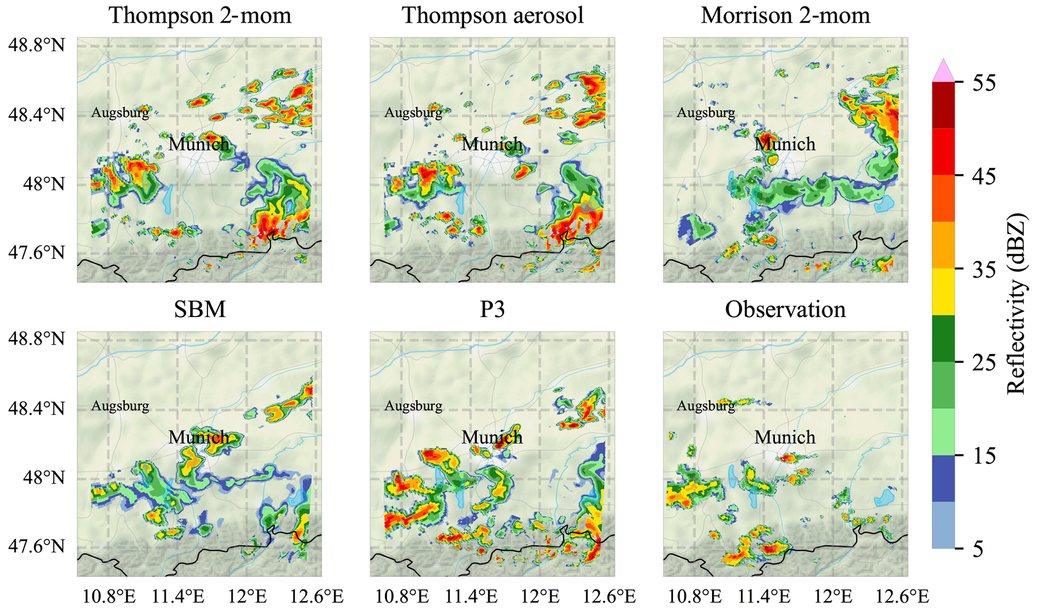
Figure 1 Simulated and measured reflectivity on 7 July 2019, 12:45 UTC, over the full domain size with a grid spacing of 400 m. Simulated reflectivity from the WRF model output after applying the CR-SIM forward simulator Oue et al. (2020). Background map tiles are by Stamen Design (Stamen Design, 2022). Background map data are by OpenStreetMap (OpenStreetMap, 2022, © OpenStreetMap contributors 2022. Distributed under the Open Data Commons Open Database License (ODbL) v1.0.). Roads, rivers, and lakes are made with Natural Earth (Natural Earth, 2022).

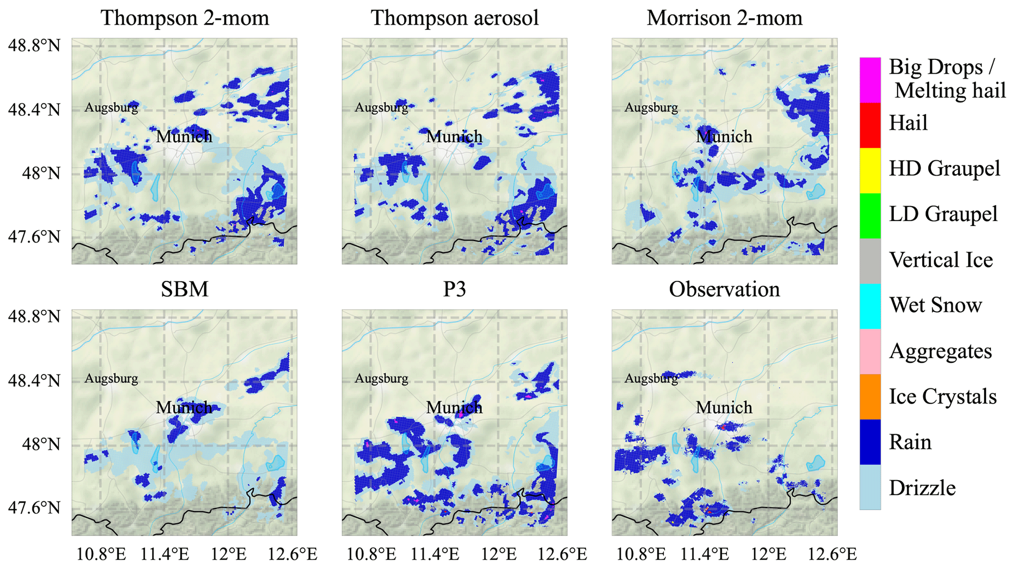
Figure 2 The same as Fig. 1 but for hydrometeor classification data, retrieved from the (simulated) polarimetric radar signals with Dolan et al. (2013). Background map tiles are by Stamen Design (Stamen Design, 2022). Background map data are by OpenStreetMap (OpenStreetMap, 2022, © OpenStreetMap contributors 2022. Distributed under the Open Data Commons Open Database License (ODbL) v1.0.). Roads, rivers, and lakes are made with Natural Earth (Natural Earth, 2022).

The weather situation chosen as an example occurred at 12:45 UTC on 7 July 2019 and was characterized by widely scattered convective showers over the Alps, directly over Munich, and in the Munich vicinity (Fig. 1). In general, all simulations at this time produce precipitation over much of the model domain. The general convective nature of the precipitation is correctly reproduced; there are numerous scattered convective cells, some isolated, in all simulations. The magnitude of the reflectivity maxima is similar to the radar observations. However, this case also shows some limitations of numerical weather prediction for convective situations: the location of the simulated convective cells does of course not exactly match the observations. The area covered by precipitation is larger than that observed in most simulations. This is mainly due to a simulated precipitation area northeast of Munich that was not observed at that time. Further, the simulated cells are smaller and more frequent, especially in the two Thompson simulations. This is not a general problem with these schemes: the total number of simulated convective cells from the Thompson schemes over all 30 d is similar to those observed, as shown in Köcher et al. (2022). It rather points out the challenge to compare observations and simulations on a single case study.

The corresponding hydrometeor classification for the same case is shown in Fig. 2. Most of the signals are classified as rain or drizzle in both the observations and all of the simulations. Embedded areas of large drops/melting hail or hail are classified in the observations and in four of the simulations: Thompson two-moment (2-mom), Thompson aerosol aware, Morrison 2-mom, and P3 are for the most part even able to produce hail cores of very similar sizes to those observed at this time. At the same time, general limitations of model predictions are also evident here: the exact location of the hail and the associated convective cell are shifted compared to the observations and also vary depending on the scheme. Not all simulations classify (melting) hail at this time step. In addition, the hail core is partially classified as dry hail in the observations, while the simulations produce mostly melting hail at this time step. This scene shows that the choice of microphysics scheme has noticeable effects on the prediction of location, time, strength, and type of convective precipitation. But is this also relevant statistically over a longer period? For a general evaluation of model prediction as a function of a microphysics scheme, a statistical analysis over a longer time period is needed.

4 Heavy-rainfall statistics

The objective of this study is to statistically evaluate microphysics schemes using polarimetric radar observations. To enable comparison between model and radar, either a radar signal must be simulated based on the model output or information about hydrometeor classes must be obtained from the observed radar signals. These two approaches are combined here to statistically compare observations and model outputs to evaluate microphysical processes related to high-impact weather events: heavy rain and hail. To define a heavy-rain or hail event, we applied the hydrometeor classification of Dolan et al. (2013) to the observed and simulated (with a radar forward operator) polarimetric signals in the same way. The frequency and area of heavy-rain and hail events defined in this way are then statistically compared to analyze differences between the model and observations and the influence of the microphysical processes. The statistics extend over 30 convection days. Since we do not have ground-based observations available due to radar elevation, we restrict all analyses to an altitude level of about 1 km above Munich. This altitude is the lowest possible altitude at which we have complete radar coverage of Munich.

4.1 Statistics based on observed and simulated reflectivity

We begin our statistical analysis with an evaluation of the frequency and area of heavy-rain events. The top row in Fig. 3 shows the frequency and area of rain events for different event strengths at an altitude of 1 km above Munich. The strength of the event is defined by the simulated or observed reflectivity. We calculate the total duration of a day when rain was classified above a certain reflectivity threshold. For our 30 d dataset, this gives a time series of 30 values. The minimum, mean, and maximum of this time series are shown in the top left of Fig. 3 for both the simulations for the five microphysics schemes and the observations. Thus, one can compare the frequency of rain of different intensities. The maximum possible time is 24 h, which would correspond to rain for an entire day (for all 288 5 min steps) above the given reflectivity threshold. For this figure, it does not matter how large the area was classified as rain during a time step as long as at least one pixel was classified as rain. The area of rain events is presented in the top right of Fig. 3. The term area here refers to the cross-section area at 1 km altitude that was covered by the rain during a time step. The maximum possible area in the figure is 1800 km², which would mean that the Munich domain is completely covered by rain above the specified threshold. Both model output and radar observations provide data every 5 min. Figure 3 shows the minimum, mean, and maximum area over all time steps where rain was classified above the corresponding threshold. The total time with any rain somewhere in the domain averages to more than 13 h in all simulations and in the observations. This high number of rain events is a consequence of the fact that our dataset consists specifically of days with convective precipitation. At the smallest reflectivity thresholds (5 and 10 dBZ), all schemes underestimate the occurrence of rain in the domain by about 5 h on average per day compared to radar observations. This weak precipitation is typically classified as drizzle. At the same time, the area of these drizzle events is larger in the simulations than in the observations. This is due to the fact that the radar observations are much more likely to show scattered and isolated grid cells classified as drizzle, while the simulations typically show somewhat larger, contiguous fields of precipitation. In part, this difference may be due to some clutter that could not be filtered out from the observations. In any case, these observed isolated drizzle clouds are usually very small and likely evaporate before they reach the ground. There are some arguments about why these drizzle events are nevertheless important, even if the precipitation does not reach the ground, such as by affecting the water balance and turbulent dynamics (Wyant et al., 2007). In addition, drizzle is often poorly represented in NWP models (Wyant et al., 2007; Wilkinson et al., 2012). However, we do not consider this issue to be the focus of this study and will not discuss it in detail.

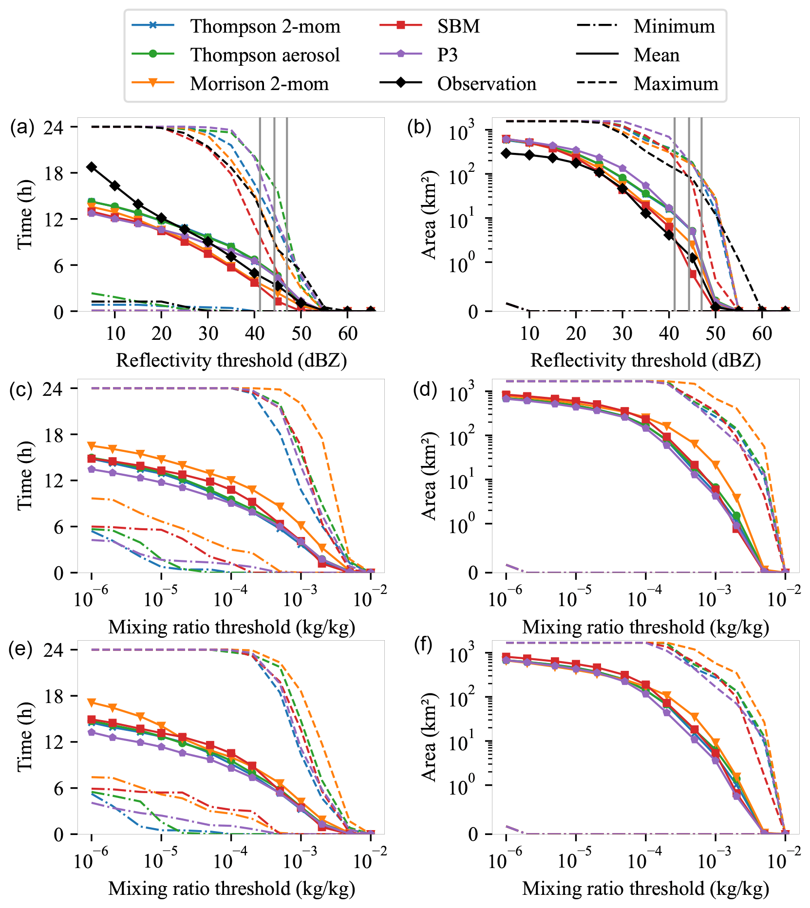
Figure 3 Frequency (a, c, e) and area (b, d, f) of classified rain above various thresholds. Minimum (dashed–dotted line), mean (solid line), and maximum (dashed line) over the 30 d dataset. Gray vertical stripes: thresholds for heavy precipitation (15, 25, and 40 mm h⁻¹) from the DWD after conversion to reflectivity (dBZ) using a Z–R relation. (a–b) Statistics based on simulated and observed reflectivity thresholds at 1 km altitude. Simulated reflectivity from WRF model output after applying the CR-SIM forward simulator (Oue et al., 2020). (c–d) Statistics based on mixing ratio thresholds at 1 km altitude. (e–f) Statistics based on thresholds for mixing ratio at the surface. The y axis on the right side is logarithmically scaled, except for a small range around 0 (0–1) with a linear scale.

The vertical gray lines in Fig. 3 show the thresholds used by the DWD for heavy rainfall (15, 25, and 40 mm h⁻¹; Deutscher Wetterdienst, 2022) after applying a Z–R relationship for convective precipitation (Woodley, 1970):

$$\begin{array}{}\text{(1)}& z=\mathrm{300}\cdot R^{\mathrm{1.4}},\end{array}$$

where R is the rain rate in mm h⁻¹ defined by the DWD, and z is the reflectivity in mm⁶ m⁻³, which is then converted into logarithmic units in decibels:

$$\begin{array}{}\text{(2)}& Z=\mathrm{10}\cdot {\log }_{\mathrm{10}}\left(z\right).\end{array}$$

The heavy-rain thresholds of 15, 25, and 40 mm h⁻¹ are thus converted to reflectivity thresholds of 41.2, 44.3, and 47 dBZ. This gives an indication of the reflectivity thresholds that correspond to heavy rain. In these ranges the cloud microphysics has a strong influence on the simulated rain events. The frequencies from the simulated heavy-rain events scatter around the observed frequency, which is pretty much in the middle of the different simulations. However, the scatter is considerable; i.e., some of the simulations differ by 4 h in mean, which corresponds to a factor of more than 2 for the 41.2 dBZ heavy-rainfall threshold and a factor of about 5 for the 44 dBZ threshold. All simulations produce rainfall areas that are, on average, larger than the observed rainfall areas, almost regardless of the reflectivity threshold. Interestingly, the same microphysics schemes that simulate heavy-rain events most frequently also simulate the largest rain areas, i.e., the simulations using the P3 scheme and the two Thompson schemes.

The most important information from this section is that most schemes produce heavy rainfall that is too large in area by a factor of up to 4. The frequency of heavy-rain events is more similar to observed events but still scatters by a factor of up to 2 around the observations. In particular, for both Thompson schemes and the P3 scheme, this is a large overestimate of heavy-precipitation events. These statistics are based on reflectivity thresholds. The question here is will this also affect the amount of precipitation, i.e., rain mass? Reflectivity is disproportionately dominated by large droplets compared to rain mass. So in order to relate these results to actual rain mass, we repeat the analysis from this section but based on thresholds for rain mass (or rain mass mixing ratio) instead of reflectivity.

4.2 Heavy-rainfall statistics based on model mass mixing ratio

In the previous part we have shown statistics of rain events of different intensities based on HID fields classified from (simulated) radar reflectivity fields. To constrain the model output with radar observations it is necessary to simulate reflectivities from the model output. A disadvantage of this procedure is that it relies on the radar forward operator. However, information about the simulated hydrometeors is also directly available in the model output in the form of the mixing ratios. In the following part, we repeat the analysis from the previous part with rain mass mixing ratio thresholds instead of reflectivity thresholds to show how the analysis in the reflectivity space is related to a direct analysis of the model output rain mass.

The middle row in Fig. 3 shows the same analysis as the top row, with the difference that this time the rain events are defined by the mixing ratio directly from the model output. The center-left image in this figure shows how often rain was simulated above different mixing ratio thresholds. The center-right image shows the covered area, following the same methodology as in the previous part. The analysis also takes place at an altitude of 1 km above the surface to guarantee comparability, even though we have the simulated mixing ratio data available at the surface as well. Most of the schemes produce distributions of rain events with a similar pattern over the different mixing ratio thresholds; actually only the Morrison scheme deviates noticeably and produces rain events of any magnitude (with respect to the mixing ratio) more frequently than the other schemes. At higher mixing ratio thresholds (> 10⁴ kg kg⁻¹), these events are also simulated over larger areas in the Morrison simulations than in the other simulations. This ultimately means that the Morrison simulations produce a significantly larger mixing ratio and especially so for the particularly intense precipitation events.

When comparing this to the top row, we find substantial differences: the schemes that overestimated heavy-precipitation events the most when based on reflectivity thresholds (P3, Thompson 2-mom, Thompson aerosol aware) simulated actually the least often heavy-precipitation events when based on direct mixing ratio thresholds. Especially the conclusion that the P3, Thompson 2-mom, and Thompson aerosol-aware simulations simulate too much heavy precipitation is not visible at all from the model mixing ratio directly. How can this discrepancy be explained? The following two reasons account for this: (1) for liquid drops, the mass mixing ratio depends to the third power (∝D³) on particle diameter, while reflectivity depends to the sixth power (∝D⁶) on particle diameter. Thus, particle size distribution plays an important role in inferring mass from reflectivity or vice versa. For example, particle size distributions with many small particles and few large particles may contribute significantly to the mass mixing ratio but very little to reflectivity. (2) The HID algorithm always returns the dominant hydrometeor class and not the mixture of all particles present in the volume. In contrast, the mixing ratio output by the model takes into account all simulated hydrometeors. This means that if rain is common in a scheme but is rarely the dominant class, then rain is strongly represented in mixing ratio analyses but poorly represented in the HID analysis.

4.3 The role of the particle size distribution

To test the hypothesis from above, we calculated the rain particle size distributions (PSDs) for all our microphysics schemes. The mean particle size distributions over all time steps and all inner domain grid boxes at 1 km are shown in Fig. 4. The spectral bin simulations provide total mixing ratios for a number of droplet size bins as direct model output. From this, the number concentration of raindrops of a given size bin is calculated by dividing the given mixing ratio by the mass of a droplet of the corresponding size bin. For the bulk schemes, we calculated the PSD according to the parameterization of the schemes by implementing the parameterization as described in the corresponding publication (Thompson et al., 2008; Morrison et al., 2009; Thompson and Eidhammer, 2014; Shpund et al., 2019; Morrison and Milbrandt, 2015), as well as directly from the code available on GitHub (Skamarock et al., 2019). Because the bulk schemes do not actually have fixed size bins, the number concentration can be calculated for any droplet size. To make the distributions comparable, we calculated the number concentrations for the bulk schemes for the droplet sizes that match the raindrop size bins of the SBM scheme. Figure 4 shows the PSD over these 18 bins. It can be seen that, on average, the SBM and Morrison schemes produce raindrops of 1 mm and smaller much more frequently (by a factor of more than 10) for small diameters. The opposite is true for large raindrops greater than 4 mm, which were not simulated at all by the SBM scheme. In principle, the SBM can simulate larger raindrops, as the largest bin corresponds to raindrops of 6.6 mm diameter. According to Shpund et al. (2019), there is a drop breakup scheme applied that follows Kamra et al. (1991) and Srivastava (1971), which includes spontaneous breakup and collisional breakup. There is also a snow breakup scheme applied, which might limit the raindrop sizes for rain created from melting snow. We therefore believe that the PSD is the main reason for the different behaviors of the schemes in the reflectivity space and mixing ratio space. The sheer amount of small droplets in the Morrison and SBM schemes thus contributes noticeably to the total mass but less to the reflectivity, which is simulated much lower in comparison, especially in the SBM scheme due to the lack of large raindrops.

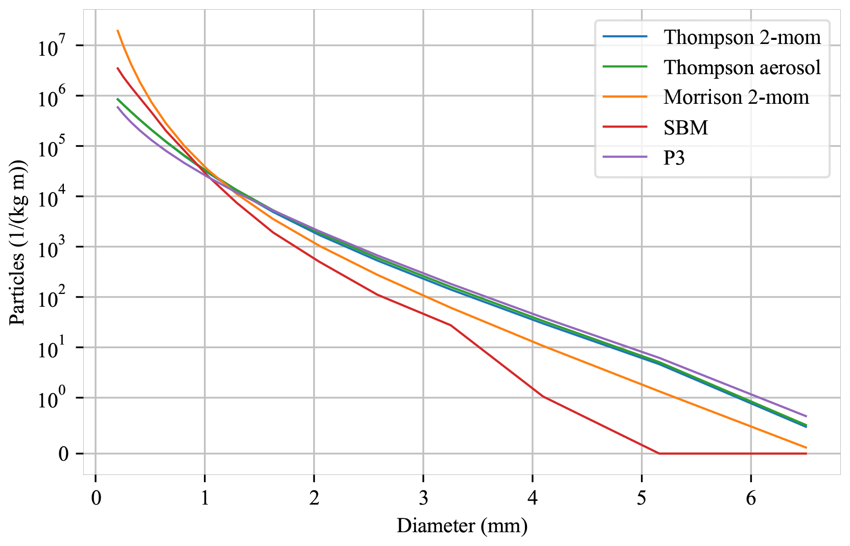
Figure 4 Mean raindrop size distribution over all 30 d at 1 km altitude. The y axis is logarithmically scaled, except for a small range around 0 (0–1) with a linear scale.

This strongly suggests that it is not the rain mass produced that is the problem with the simulations but rather the distribution of mass across droplet sizes. We cannot say with certainty what the particle size distributions looked like in reality during our 30 d dataset because we do not have direct measurements of the droplet size distribution. But given that the SBM scheme simulates a high mixing ratio of rain mass, but at the same time produces too few heavy-rain events based on the reflectivity produced, it stands to reason that this scheme generally produces too few large raindrops. The exact opposite is true for the P3, Thompson 2-mom, and Thompson aerosol-aware simulations. These results are consistent with the findings of Köcher et al. (2022), where the simulated differential reflectivity was statistically compared with the observed one. In particular, the SBM scheme did not produce larger differential reflectivity in the lower elevations, suggesting the absence of large drops in the SBM, while the P3 and Thompson schemes produced large differential reflectivity signals too frequently. A similar comparison of polarimetric radar signatures was performed by Wu et al. (2021) for a typhoon precipitation event in 2016. They noted that none of their simulations were able to successfully reproduce the observed polarimetric radar signatures. This was attributed to median raindrop sizes that are too large (Morrison and Thompson schemes) and a simulated frequency of very large raindrops lower than observed (Thompson scheme). In contrast, Putnam et al. (2016) found that both Morrison and Thompson 2-mom produce reflectivity values that are too high, which they attributed to PSDs containing too many large drops; too much precipitation coverage; and, in the case of the Morrison simulations, a bias due to wet graupel. With respect to our study, we can confirm too much precipitation coverage, and our results suggest that there are too many large raindrops in the Thompson simulations, which is consistent with Putnam et al. (2016) but in contrast to Wu et al. (2021). However, both studies evaluated the microphysics schemes using only case studies, which is not generally applicable to different weather situations. This shows an advantage of our statistical approach, which allows for more robust conclusions.

The analysis to this point has been limited to an altitude of 1 km above the surface, limited by the radar observations. However, another question remains: does the analysis at 1 km altitude translate to precipitation at the surface? Precipitation on its way to the ground is affected by processes such as evaporation and drop sedimentation, and different microphysics schemes treat these processes differently. Therefore, we repeat the mixing ratio analysis again but with data from the surface to relate the results from 1 km altitude to results at the surface.

4.4 Rain mass mixing ratio analysis at the surface

The bottom row in Fig. 3 shows the same analysis as the center row, except that this time surface mixing ratios are analyzed instead of 1 km altitude. We find that at the surface, the Morrison and SBM simulations showed the most frequent and most widespread rain events, throughout most mixing ratio thresholds. This is in general agreement with the analysis at 1 km height. However, the difference, especially between the Morrison and other schemes, becomes smaller. This suggests that rain within the Morrison scheme undergoes stronger evaporation compared to the others. Given that the Morrison scheme produced on average the highest number of very small raindrops of 0.5 mm and smaller at 1 km altitude, a high evaporation rate is to be expected. Since the general ranking between the schemes is almost the same between 1 km altitude and the surface, we argue that findings at 1 km altitude are a good proxy for the surface. However, the difference between the schemes at the surface definitely becomes smaller, and all schemes produce a frequency and area of rain events of similar magnitude.

Summarizing the results of the rainfall statistics, we can note the following: all schemes overestimate the area of heavy-rain events based on reflectivity thresholds; P3 and the two Thompson schemes also overestimate the frequency of heavy-rain events, while the SBM and Morrison schemes underestimate the frequency of heavy-rain events. Further analysis of the rain mixing ratio and the calculated particle size distributions indicates that large raindrops that contribute strongly to high reflectivities are simulated too frequently in the P3, Thompson 2-mom, and Thompson aerosol-aware simulations, while large raindrops occur too infrequently in the SBM simulations.

5 Hail and graupel statistics

So far, the focus has exclusively been on heavy-rain events. However, hail events also have damage potential and therefore are of interest. The P3 scheme does not have a separate hail or graupel class. Therefore, to allow for a fair comparison between the schemes, we included all ice in this analysis. Given that the dataset consists of convective cases mainly in summer, most of the ice present at 1 km altitude and below is graupel- or hail-like anyway. For completeness, the analysis restricted to graupel and hail only (and thus without the P3 scheme) is provided in the Supplement.

5.1 Statistics based on observed and simulated reflectivity

Figure 5 shows the area and frequency of these ice events in the same manner as Fig. 3 for rain. The choice of microphysics scheme has a significant impact on the ice statistics, across all reflectivity thresholds. The most extreme case is the SBM scheme, which hardly produces any ice events at higher reflectivities. There is not a single time step within the 30 d dataset at which the SBM scheme simulated ice grid cells of 35 dBZ or higher (top-left image in Fig. 5). However, most of the other schemes, and especially the Morrison scheme, also consistently show fewer ice events compared to the observations. Unlike the rain analysis, this is consistent across all reflectivity thresholds and not limited to the lower reflectivities. Only the P3 scheme is similar in terms of frequency, and for it only the highest reflectivity events (≥55 dBZ) are too rare. None of the simulations, regardless of the cloud microphysics scheme, were able to reproduce these extreme events. This can have multiple reasons.

• Model resolution. Such high reflectivities require very large particles. For hail formation, for example, strong updrafts must be present. There is some discussion about the grid spacing required to properly represent these updrafts. Lebo and Morrison (2015) and Jeevanjee (2017), for example, show that a grid spacing less than about 250 m is required before some convective storm characteristics such as vertical velocity or convective core area converge; i.e., further decreasing the grid spacing has only a limited effect. This means that even our grid spacing of 400 m, which is much better than current weather models, may still be too large to correctly simulate the strongest hail events.

• Particle density. The particle density strongly influences the reflectivity. All schemes except the P3 scheme consider graupel particles with constant density of 400–500 kg m⁻³ and do not explicitly calculate hail.¹ Hail particles, however, are typically much denser than graupel. This means if hail events are observed, the high hail density can lead to high observed reflectivities that cannot be reproduced by the simulations due to the lower assumed particle density. Only the P3 scheme has a more flexible approach that allows varying ice particle density reaching up to 900 kg m⁻³.

• Melting particles. The microphysics schemes applied do not consider particles that are partially melted; all particles are either completely frozen or completely melted.² The radar forward operator CR-SIM does not apply a melting scheme either. That means it is impossible not only to reproduce certain radar signatures related to melting (e.g., a bright band), but also to simulate the increase in reflectivity due to partially melted hail particles. The highest reflectivity events observed could be due to partially melted hail particles, which would translate to an increase in reflectivity that is not reproducible by the schemes applied in this study.

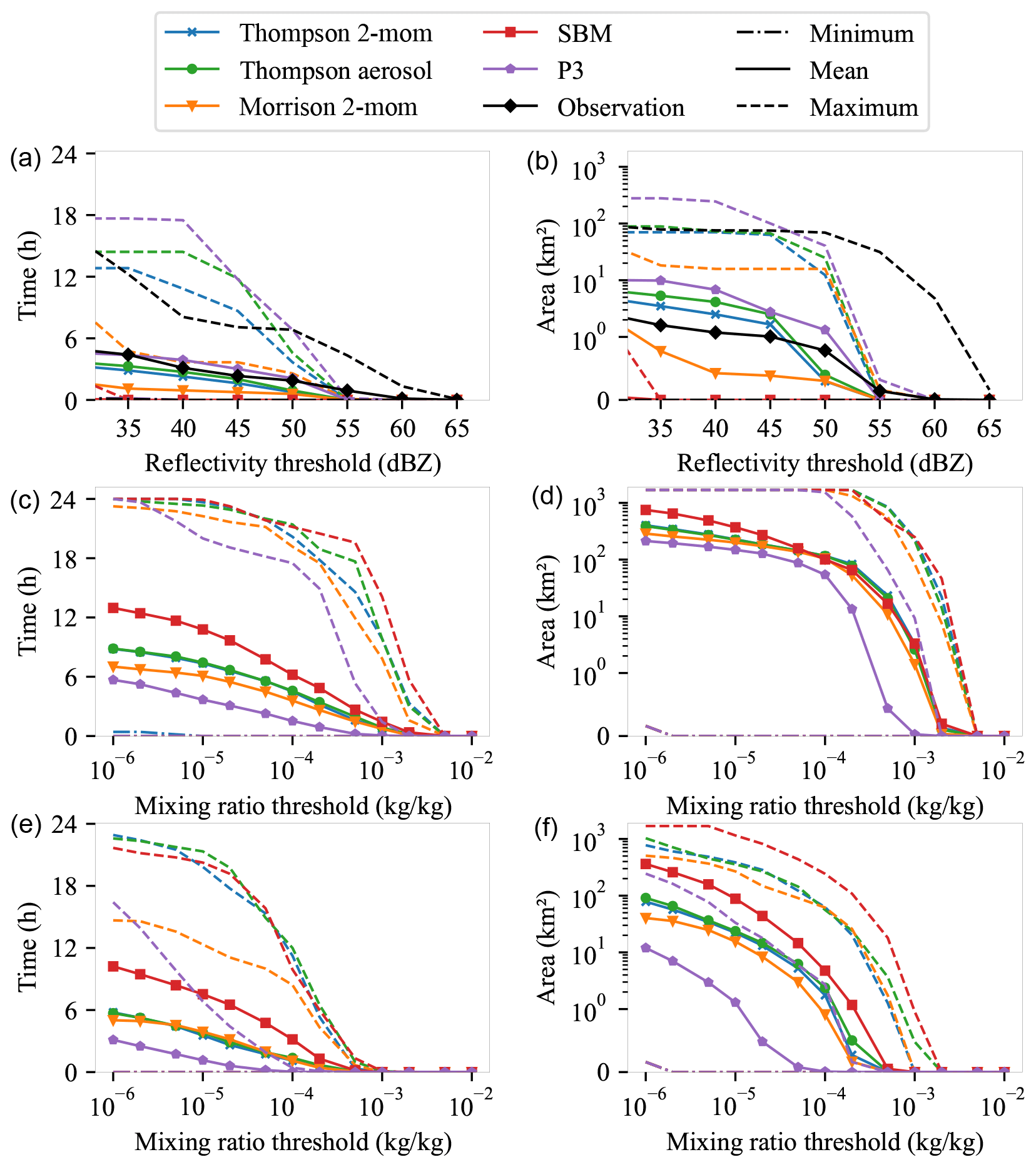
Figure 5 The same as Fig. 3 but for ice statistics. Frequency (a, c, e) and area (b, d, f) of ice events above various thresholds. Minimum (dashed–dotted line), mean (solid line), and maximum (dashed line) over the 30 d dataset. (a–b) Statistics based on simulated and observed reflectivity thresholds at 1 km altitude. Simulated reflectivity from WRF model output after applying the CR-SIM forward simulator (Oue et al., 2020). (c–d) Statistics based on mixing ratio thresholds at 1 km altitude. (e–f) Statistics based on thresholds for the mixing ratio at the surface. The y axis on the right side is logarithmically scaled, except for a small range around 0 (0–1) with a linear scale.

We note, however, that most schemes are quite capable of producing events of this magnitude at reflectivity thresholds of about 45 and 50 dBZ. However, most schemes underestimate the frequency and area of these events compared to radar observations. With a reflectivity threshold of 50 dBZ (which may be, in part, hail events), the P3 scheme is the only one capable of producing similar statistics in terms of area and frequency of hail/graupel events. The main difference between the P3 scheme and the other schemes is that instead of predicting the moments of multiple ice hydrometeor classes (including hail and graupel), this version of the P3 scheme uses only one ice class and instead predicts the properties of that ice class, such as the fraction of rime mass. This is more flexible and may better reflect the variability of real ice particles. With the configuration that was used in this study, P3 is also the only scheme that allows ice particles to reach densities up to 900 kg m⁻³, i.e., to simulate hail-like particles. While the Thompson 2-mom and Thompson aerosol-aware simulations are at least able to reproduce the ice statistics at lower reflectivity thresholds, Morrison and SBM produce too few and too small ice events regardless of reflectivity threshold. The reasons for this are likely differences in particle size distributions in both cases. Morrison and SBM generally produce much lower reflectivity values, presumably because again the larger particles are absent. However, graupel density assumptions could also play a role. Both Morrison and SBM assume a graupel density of 400 kg m⁻³, which is slightly lower than assumed by the Thompson schemes with 500 kg m⁻³.

Again, the question arises as to how statistics based on radar reflectivity translate to statistics based on mass mixing ratio. Therefore, we continue with the analysis of ice in terms of mixing ratio, following the same structure as in the section on rain.

5.2 Hail and graupel statistics based on model mass mixing ratio

The middle row of Fig. 5 shows the same analysis as the top row but this time for the model's initial ice mixing ratios. A clear ranking can be seen between the microphysics schemes, both for area and for the frequency of ice events, which is almost independent of the mixing ratio threshold: the SBM simulations produced the most frequent and widespread ice events on average, while P3 produced ice events that were the smallest and least frequent. The majority of the ice events at the height of 1 km are graupel events because slower-falling ice, like aggregates or cloud ice, melts before it reaches the 1 km altitude. Comparing the mixing ratio analysis to the frequency and area statistics based on reflectivity in the previous section, we again see a stark contrast, especially for the P3 scheme, where ice events are most common when obtained from radar reflectivity, and for the SBM scheme, where ice events are least common. Only for the Morrison scheme do we find ice events less frequently, regardless of mixing ratio or reflectivity analysis. The SBM scheme, on the other hand, is again likely missing the larger particles, since a large mass of ice particles is generated, but this does not translate into high reflectivities.

The ice statistics from this section were performed at 1 km altitude to ensure comparability with radar observations. Again, the question is whether the results from this section can be extrapolated to the surface. Therefore, we repeat the mixing ratio analysis at the surface.

5.3 Hail and graupel mass mixing ratio analysis at the surface

The bottom row in Fig. 5 shows the same analysis as the middle row, except that this time the mixing ratio is analyzed at the surface rather than at 1 km altitude. It can be seen that the SBM scheme at the surface simulates the most frequent and widespread ice events, regardless of the reflectivity threshold, followed by the two Thompson schemes and the Morrison scheme. The least frequent and also the smallest ice events are simulated by the P3 scheme. This ranking is the same as at 1 km altitude, indicating that the findings from 1 km altitude are approximately applicable to the surface as well. However, the P3 scheme simulates much smaller areas of ice at the surface than at 1 km altitude. This suggests that the melting process in the P3 scheme is stronger than in the other schemes. However, since we do not have measurements of the particle size distribution at the surface, we cannot say whether these high melting rates are realistic.

In summary, for the ice statistics, no scheme is able to reproduce the most extreme reflectivity statistics of greater than 55 dBZ, which might be a problem with density assumptions, the absence of partially melted particles in the simulations, or resolution. Hail/graupel at reflectivity thresholds of 45 to 50 dBZ is correctly reproduced only by the P3 scheme. The other schemes, especially Morrison and SBM, underestimate the frequency and area of ice events regardless of reflectivity threshold. Analysis of the ice mixing ratio directly from the model output suggests that the SBM scheme produces a high ice mixing ratio, but this is not correctly distributed over the particles sizes, and the larger graupel particles are likely missing.

6 Summary and conclusions

In this study, microphysics schemes of varying complexity are evaluated via statistical comparison with polarimetric C-band radar observations. The focus is on the statistics of high-impact weather events, i.e., hail and heavy precipitation. The dataset consists of 30 convective days during the summers of 2019 and 2020. The radar observations consist of polarimetric volume scans from the C-band radar at Isen, which is operated by the German Weather Service (DWD). The same days are simulated using a convection-permitting Weather Research and Forecasting (WRF) model setup over Munich with a horizontal grid spacing of 400 m, 40 vertical levels, and 5 different microphysics schemes of varying complexity. The radar forward operator CR-SIM (Oue et al., 2020) is applied to the model results and yields simulated polarimetric radar signals, consistent with the corresponding microphysics schemes. The hydrometeor classification algorithm of Dolan et al. (2013) is applied to simulated as well as observed radar signals to identify dominant hydrometeor classes and define heavy-rain or ice events. Frequencies and areas of these events from the radar observations are then compared to the simulations to evaluate the microphysics schemes.

Analysis of the heavy-rain events shows that all simulations, regardless of the microphysics scheme, overestimate the area of the heavy-rain events based on the reflectivity thresholds compared to radar observations. Since this is independent of the microphysics scheme, we suspect that this is not an issue of the microphysics but rather related to the limited grid resolution: the simulations tend to produce larger, contiguous precipitation fields, whereas in reality precipitation fields are sometimes more scattered and small. With respect to the frequency of heavy-rainfall events, there is significant scatter between simulations: the P3, Thompson aerosol-aware, and Thompson 2-mom schemes overestimate the frequency of heavy-rain events by a factor of up to 2 compared to radar observations, while the spectral bin (SBM) scheme underestimates the frequency of heavy-rain events by a factor of up to 2. This means that the P3 and both Thompson schemes greatly overestimate both the frequency and area of heavy rain based on reflectivity thresholds. To apply these results to rain mass, an analysis of the same statistics was performed based on the mixing ratio of rain mass in the model. In contrast to the reflectivity analysis, the P3, Thompson aerosol-aware, and Thompson 2-mom schemes produce the fewest heavy-rainfall events and the smallest in area. Analysis of the simulated rain particle size distributions shows that the Morrison and SBM schemes on average produce more small raindrops of 1 mm and smaller by a factor of up to 10, while at the same time the SBM scheme simulates the fewest large raindrops. We conclude that it is not the rain mass produced that is the problem but rather the distribution across droplet sizes: compared to the radar-observed heavy-rain events, the P3, Thompson 2-mom, and Thompson aerosol-aware schemes produce large raindrops too frequently, while the SBM simulations produce too few. The results related to the Thompson 2-mom and Morrison schemes are in conflict with a previous study by Wu et al. (2021) but are consistent with Köcher et al. (2022) and Putnam et al. (2016), highlighting the problem of evaluating microphysics schemes using case studies and demonstrating the importance of statistical evaluation as in this study.

Similarly, we repeated the analysis for summer ice events, assuming that they represent the hail and graupel risk at the surface. We note that none of our simulations is able to reproduce the radar observations at the highest reflectivity thresholds 55 dBZ and above. This might be related to (1) limitations due to model resolution, (2) density assumptions that are not representative of high-density hail-like particles, or (3) the absence of partially melted particles in the simulations. For slightly smaller reflectivity thresholds of 45 dBZ to 50 dBZ, the schemes are partially able to simulate events of this magnitude. However, only the P3 scheme is able to reproduce the frequency and area of hail/graupel events of this magnitude very closely to the statistics observed by radar. All other schemes, particularly the Morrison and SBM schemes, underestimate the frequency and area of ice events, regardless of reflectivity threshold. Analysis of the model's ice mixing ratio shows that of the SBM and Morrison schemes, only the Morrison scheme simulates a low mass of ice on average. The SBM scheme, on the other hand, simulates the largest mass of ice. Thus, we conclude that the SBM scheme does not correctly distribute the mass over the particle sizes; the large particles are missing.

Relating radar-derived weather statistics to precipitation statistics at the surface is challenging. Although the simulations suggest that the mixing ratio at 1 km altitude is strongly related to the mixing ratio – and hence precipitation rate – at the ground, there are processes such as evaporation, drop breakup, or self-collection that affect this. In special cases, it is certainly possible for these processes to significantly change the precipitation rate. Therefore, one always has to rely on a model that correctly simulates these processes when radar measurements are used to make statements about precipitation on the ground. Furthermore, we used a radar forward simulator for the analysis in this study. This is a useful tool to simulate the expected radar signals using the model data. However, it makes broad assumptions about the aspect ratio, orientation, shape, and density of the particles. Therefore, the application of these rigid relations inevitably results in the simulated particle properties not exhibiting the same variability as in nature. Furthermore, in this study, we applied a hydrometeor classification algorithm to classify the predominant hydrometeors in the radar observation volumes. This algorithm is based on theoretical scattering simulations, and only the dominant hydrometeor class is determined. This makes it difficult to relate the radar-based results to precipitation rates. It would be very helpful if, in addition to the dominant hydrometeor class, the corresponding mixing ratio was also derived from the polarimetric radar variables. Within a sub-project of the German Research Foundation (DFG) Priority Programme 2115 (PROM, Trömel et al., 2021), an HMC algorithm is currently being developed for this purpose. This algorithm is based on a clustering approach and an algorithm for quantifying the mixing ratio following Grazioli et al. (2015), Besic et al. (2016), and Besic et al. (2018) and aiming to calculate the mixing ratios of hydrometeor classes as well. Thus, mixing ratios derived from the radar signal could be directly compared with the mixing ratios simulated by the model.

Can numerical weather prediction (NWP) forecasts be further improved by applying more complex microphysics schemes? Our analysis of high-impact weather events does not show a clear advantage of more complex schemes; there are significant deviations from observations for all of the schemes applied. Simply increasing the complexity does not necessarily improve predictions. Novel observations are needed to provide the necessary information and better constrain the microphysical processes. In this work we have shown the potential of polarimetric radar observations to do just that and suggest they be further explored.