Unbalanced emission reductions of different species and sectors in China during COVID-19 lockdown derived by multi-species surface observation assimilation

The unprecedented lockdown of human activities during the COVID-19 pandemic has significantly influenced social life in China. However, understanding the impact of this unique event on the emissions of different species is still insufficient, prohibiting the proper assessment of the environmental impacts of COVID-19 restrictions. Here we developed a multi-air-pollutant inversion system to simultaneously estimate the emissions of NO_x, SO₂, CO, PM_2.5 and PM₁₀ in China during COVID-19 restrictions with high temporal (daily) and horizontal (15 km) resolutions. Subsequently, contributions of emission changes versus meteorological variations during the COVID-19 lockdown were separated and quantified. The results demonstrated that the inversion system effectively reproduced the actual emission variations in multi-air pollutants in China during different periods of COVID-19 lockdown, which indicate that the lockdown is largely a nationwide road traffic control measure with NO_x emissions decreasing substantially by ∼40 %. However, emissions of other air pollutants were found to only decrease by ∼10 % because power generation and heavy industrial processes were not halted during lockdown, and residential activities may actually have increased due to the stay-at-home orders. Consequently, although obvious reductions of PM_2.5 concentrations occurred over the North China Plain (NCP) during the lockdown period, the emission change only accounted for 8.6 % of PM_2.5 reductions and even led to substantial increases in O₃. The meteorological variation instead dominated the changes in PM_2.5 concentrations over the NCP, which contributed 90 % of the PM_2.5 reductions over most parts of the NCP region. Meanwhile, our results suggest that the local stagnant meteorological conditions, together with inefficient reductions of PM_2.5 emissions, were the main drivers of the unexpected PM_2.5 pollution in Beijing during the lockdown period. These results highlighted that traffic control as a separate pollution control measure has limited effects on the coordinated control of O₃ and PM_2.5 concentrations under current complex air pollution conditions in China. More comprehensive and balanced regulations for multiple precursors from different sectors are required to address O₃ and PM_2.5 pollution in China.

1 Introduction

A novel coronavirus disease (COVID-19) broke out in Wuhan at the end of 2019 but quickly spread across the whole of China within a month. To curb the spread of the virus, strict epidemic control measures were implemented by the Chinese government to prevent large gatherings, including strict travel restriction, shutting down non-essential industries, extended holidays, and the closing of schools and entertainment establishments (Cheng et al., 2020). These restrictions have had a significant impact on industrial activities and social lives, as exemplified by the drop in China's industrial output by 15 %–30 % (https://data.stats.gov.cn/, last access: 22 October 2022) and the dramatic decrease in traffic flow by 60 %–90 % in major cities of China during the COVID-19 epidemic (http://jiaotong.baidu.com/, last access: 22 October 2022), which provides us a natural experiment to examine the responses of the emissions and air quality on the changes in human activities.

It has been well documented that the short-term stringent emission controls targeted on power generation and heavy industry enacted by the Chinese government during certain societal events, such as the 2008 Olympics Games, 2014 Asia-Pacific Economic Cooperation conference and 2015 China Victory Day parade, are an effective way to reduce emissions and improve air quality (Okuda et al., 2011; Wang et al., 2014; Tang et al., 2015; Zhang et al., 2016; Wu et al., 2020; Chu et al., 2018). However, different from those stringent emission controls, the COVID-19 restrictions are inclined to affect emissions from sectors more closely to social life whose influence on emissions has still not been well assessed. Previous studies suggest that the COVID-19 restrictions have substantially reduced China's anthropogenic emissions from almost all sectors (Zheng et al., 2021; Huang et al., 2021; Xing et al., 2020). For example, by using a bottom-up method based on near-real-time activity data, Zheng et al. (2021) reported that the emissions of NO_x, SO₂, CO and primary PM_2.5 decreased by 36 %, 27 %, 28 % and 24 % during COVID-19 restrictions, mostly due to the reductions in the industry and transportation sectors. Xing et al. (2020), by using a response model, estimated stronger COVID-19 shutdown effects on emissions over the North China Plain (NCP) with emissions of NO_x, SO₂ and primary PM_2.5 dropping by 51 %, 28 % and 63 %, respectively. Others argue that the COVID-19 restrictions may mainly affect the emissions from transportation, light industry and manufacturing, while they have much smaller effects on the emissions from power generation and heavy industry because of their non-interruptible processes (Chu et al., 2021; Hammer et al., 2021; Le et al., 2020; Zhao et al., 2020). Moreover, the residential emissions may even increase during the COVID-19 lockdown due to the increased demand for space heating and cooking with the stay-at-home orders. Therefore, Le et al. (2020) only considered the NO_x reductions during COVID-19 restrictions in their investigation of the severe haze during the COVID-19 lockdown, and similarly, Hammer et al. (2021) only considered the emission reductions in the transportation sector. This indicates that there is large uncertainty in the current understanding of the effects of COVID-19 restrictions on the emissions of different species.

Quantification of the emission changes in different species and different sectors during the COVID-19 lockdown is thus necessary for the comprehensive understanding of the environmental impacts of COVID-19 restrictions. In particular, although observations indeed show decreases in air pollutant concentrations during COVID-19 restrictions (Fan et al., 2020; Wang et al., 2021; He et al., 2020; Shi and Brasseur, 2020), the air quality improvement is much smaller than expected (Shi et al., 2021; Diamond and Wood, 2020; Yan et al., 2022). Moreover, severe haze still occurred in northern China (Sulaymon et al., 2021; Le et al., 2020), and O₃ concentrations even showed significant increases (Zhang et al., 2021; Li et al., 2020). A number of studies were conducted to explain this anomalistic air quality change by analyzing the effects of emission changes, meteorological variations and secondary production (Huang et al., 2021; Le et al., 2020; Hammer et al., 2021; Zhao et al., 2020, 2021; Sulaymon et al., 2021; Wang et al., 2020; Li et al., 2021). However, due to the unknown emission changes during COVID-19 restrictions, the emission reduction scenarios used to represent the COVID-19 shutdown effects varied among different studies and did not consider the spatial and temporal heterogeneity of the emission changes, leading to biases in the model simulation (Zhao et al., 2021; Li et al., 2021; Hammer et al., 2021; Zheng et al., 2021) and uncertainty in the quantification of the contributions of different factors.

Pioneer studies by Zheng et al. (2021) and Forster et al. (2020) have derived multi-air-pollutant emissions from social activity data using a bottom-up method, but due to the lack of detailed social activity data, large uncertainties existed in their estimates. The meteorologically and seasonally driven variability in the concentrations of air pollutants also prohibits drawing fully quantitative conclusions on the changes in emissions based on observations alone (Levelt et al., 2022). The emission inversion technique, which takes advantage of the chemical transport model (CTM) and real-time observations, provides an attractive way to estimate the sector-specific and space-based emission changes during COVID-19 restrictions, as shown in Zhang et al. (2020, 2021), Feng et al. (2020), and Hu et al. (2022). However, these studies only inversed the emissions of single species (e.g., NO_x and SO₂) without insights into multiple species. In view of this discrepancy, in this study we developed a multi-air-pollutant inversion system to simultaneously estimate the multi-air-pollutant emissions in China, including NO_x, SO₂, CO, PM_2.5 and PM₁₀, during the COVID-19 restrictions using an ensemble Kalman filter (EnKF) and surface observations from the China National Environmental Monitoring Centre (CNEMC). Subsequently, the inversed emission inventory was used to quantify the contributions of emission changes versus meteorological variations to the changes in PM_2.5 and O₃ concentrations over the NCP region during the COVID-19 restrictions.

2 Method and data

We developed a high-resolution multi-air-pollutant inversion system to estimate the daily emissions of NO_x, SO₂, CO, PM_2.5 and PM₁₀ in China from 1 January to 29 February 2020 when the COVID-19 pandemic was at its most serious and the effects of the COVID-19 restrictions were most profound in China. This system uses the NAQPMS (Nested Air Quality Prediction Modelling System) model as the forecast model and the EnKF coupled with the state argumentation method as the inversion method. It has the capabilities of the simultaneous inversion of multi-air-pollutant emissions at high temporal (daily) and spatial (15 km) resolutions. An iteration inversion scheme was also developed in this study to address the large biases in the a priori emissions. In order to better characterize the emission changes during the COVID-19 restrictions, the whole time period was divided into three periods according to different control phases of COVID-19 and the timing of the Chinese Lunar New Year: before lockdown (P1, 1–20 January), lockdown (P2, 21 January–9 February) and after back-to-work days (P3, 10–29 February). Emission changes in different regions of China were also analyzed, including the North China Plain (NCP), northeast China (NE), southeast China (SE), southwest China (SW), northwest China (NW) and central regions (defined in Fig. 1), to investigate the responses of emissions to the COVID-19 restrictions in different regions. In the following sections, we briefly introduce each component of the inversion system.

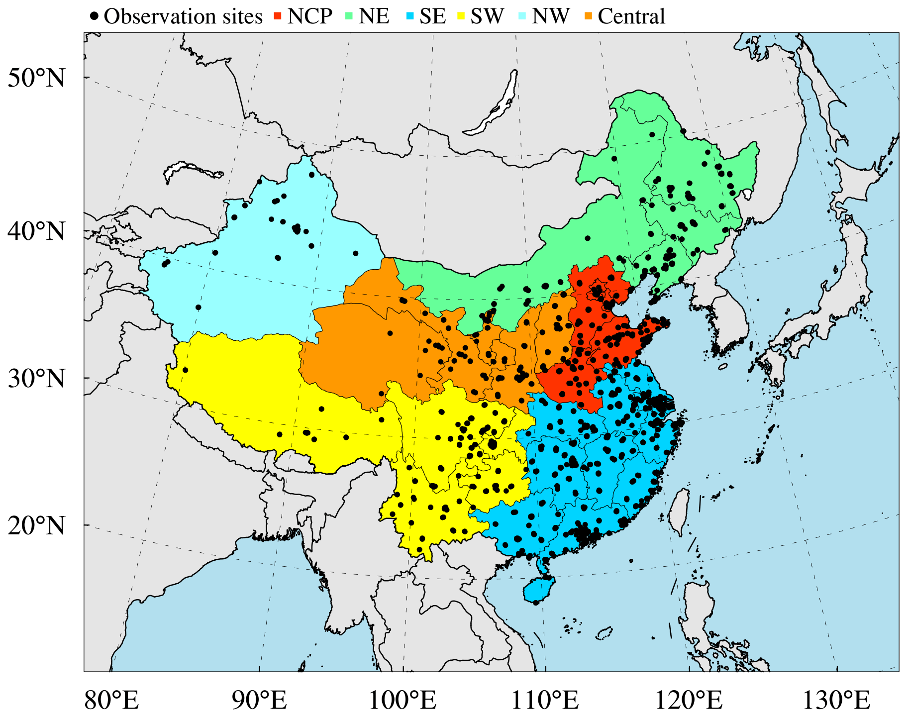
Figure 1 Modeling domain of the ensemble simulation overlaying the distributions of observation sites from CNEMC. Different colors denote the different regions in mainland of China, namely the North China Plain (NCP), northeast China (NE), southwest China (SW), southeast China (SE), northwest China (NW) and central.

2.1 Chemical transport model and its configuration

The NAQPMS model was used as the forecast model to represent the atmospheric chemistry in this study, which has been used in previous inversion studies (Tang et al., 2011, 2013; Kong et al., 2019; Wu et al., 2020), where detailed descriptions of NAQPMS are available. The Weather Research and Forecasting Model (WRF) (Skamarock, 2008) is used to provide the meteorological inputs to the NAQPMS model.

Figure 1 shows the modeling domain of this study with a high horizontal resolution of 15 km. The a priori emission inventory used in this study includes monthly anthropogenic emissions from the HTAP_v2.2 emission inventory for the base year of 2010 (Janssens-Maenhout et al., 2015), biomass burning emissions from the Global Fire Emissions Database (GFED) version 4 (Randerson et al., 2017; Van Der Werf et al., 2010), biogenic volatile organic compound (BVOC) emissions from MEGAN-MACC (Sindelarova et al., 2014), marine volatile organic compound emissions from the POET database (Granier et al., 2005), soil NO_x emissions from the regional emission inventory in Asia (Yan et al., 2003) and lightning NO_x emissions from Price et al. (1997). Chemical top and boundary conditions were provided by the global CTM MOZART (Model for Ozone and Related Chemical Tracers) (Brasseur et al., 1998; Hauglustaine et al., 1998). We assumed no monthly variations in the a priori emission inventory and used January's emission inventory for the whole simulation period so that the emission variation was solely derived from the surface observations. A 2-week free run of NAQPMS was conducted as a spin-up time. For each day's meteorological simulation, a 36 h free run of WRF was conducted, of which the first 12 h simulation was a spin-up run and the next 24 h simulation provided the meteorological inputs to NAQPMS. Initial and boundary conditions for the meteorological simulation were provided by the $\mathrm{1}{}^{\circ }\times \mathrm{1}{}^{\circ }$ reanalysis data of the National Center for Atmospheric Research and National Centers for Environment Prediction (NCAR/NCEP). Evaluation results for the WRF simulation are available in Text S1 in the Supplement.

2.2 Surface observations

The hourly concentrations of NO₂, SO₂, CO, PM_2.5 and PM₁₀ from CNEMC were used in this study to estimate the emissions during COVID-19. The spatial distributions of these observation sites are shown in Fig. 1, which contains 1436 observation sites covering most regions of China. Before assimilation, outliers of observations were first filtered out using the automatic outlier detection method developed by Wu et al. (2018) to prevent the adverse effects of the outliers on data assimilation. Then, the hourly concentrations were averaged to the daily values for the inversions of daily emissions.

The observation error is one of the key inputs to the data assimilation, which together with the background error determines the relative weights of the observation and background values on the analysis. The observation error includes measurement error and representativeness error. The measurement error of each species was designated according to the officially released documents of the Chinese Ministry of Ecology and Environmental Protection (HJ 193-2013 and HJ 654-2013, available at http://www.cnemc.cn/jcgf/dqhj/, last access: 22 October 2022), which is 5 % for PM_2.5 and PM₁₀ and 2 % for SO₂, NO₂ and CO. A representativeness error arises from the different spatial scales that the discrete observation data and model simulation represent, which was estimated based on the previous study by Li et al. (2019) and Kong et al. (2021). It should be noted that the NO₂ measurements from CNEMC are made with a chemiluminescent analyzer with a molybdenum converter. Due to the interference of HNO₃, PAN (peroxyacetyl nitrate) and alkyl nitrates (ANs), the NO₂ concentrations can be overestimated (Dunlea et al., 2007; Lamsal et al., 2008), which may lead to spurious decreases in NO_x emissions during the lockdown period. Previous studies usually use a chemical transport model to simulate NO_x, HNO₃, PAN and AN to produce correction factors (CFs) for the NO₂ measurements (Cooper et al., 2020; He et al., 2022) using the following relationship proposed by Lamsal et al. (2008):

$$\begin{array}{}\text{(1)}& \mathrm{CF}={\displaystyle \frac{\left[{\mathrm{NO}}_{\mathrm{2}}\right]}{\left[{\mathrm{NO}}_{\mathrm{2}}\right]+\mathrm{0.95}\left[\mathrm{PAN}\right]+\mathrm{0.35}\left[{\mathrm{HNO}}_{\mathrm{3}}\right]+\sum \left[\mathrm{AN}\right]}},\end{array}$$

but the calculation of CF could be affected by the simulation errors in the model caused by uncertainties in the emission inventory or other error sources which may contaminate the observations. Therefore, similar to Feng et al. (2020), we did not correct the NO₂ measurements in our inversion of NO_x emissions since there were large uncertainties in the NO_x emissions during the COVID-19 pandemic that possibly led to erroneous CFs. Since the EnKF considered the errors in observations through the use of an observation error covariance matrix, the chemiluminescence monitor interference to the NO₂ measurements was treated as the observation error during the assimilation. A sensitivity inversion experiment was also conducted based on the corrected NO₂ measurements using CFs, which suggests that the chemiluminescence monitor interference only has small impacts on the inversed NO_x emissions in terms of magnitude and its variation during the COVID-19 pandemic. Detailed results of the sensitivity experiment are available in Text S2.

2.3 Inversion estimation scheme

The EnKF coupled with the state augmentation method was used in this study to constrain the emissions of multiple species. EnKF is an advanced data assimilation method proposed by Evensen (1994) that features the representation of the uncertainties of the model state by a stochastic ensemble of model realizations. Different from the mass balance method used in Zhang et al. (2020, 2021) that has difficulties in accounting for nonlinear relationships between emissions and concentrations and is more suitable for short-lived species (e.g. NO_x) under relatively coarse ($>\mathrm{1}{}^{\circ }$) resolutions (Streets et al., 2013), the EnKF can consider the indirect relationship between emissions and concentrations caused by complex physical and chemical processes in the atmosphere through the use of flow-dependent background error covariance produced by ensemble CTM forecasts (Evensen, 2009; Miyazaki et al., 2012). Compared with the four-dimensional variational assimilation method used in Hu et al. (2022), the EnKF method has comparable computational cost (Skachko et al., 2014) but is more easily implemented without the need to develop complicated adjoint models for complex CTMs. The state augmentation method is a commonly used parameter estimation method (Tandeo et al., 2020), in which the emissions of multiple species are treated as a state variable and are simultaneously updated according to the relationship between the emissions and concentrations of related species. Due to the chemical reactions in the atmosphere, the concentrations of different species are interrelated with each other. For example, the ambient PM_2.5 is not only primarily emitted but also formed secondarily through reactions with several gaseous precursors, such as NO₂ and SO₂. This means that the estimations of PM_2.5 emissions by the single inversed estimation method could be biased if the errors in NO₂ and SO₂ emissions were not corrected synchronously. Therefore, it is beneficial to do the multi-species inversion estimation which can provide more constraints on the atmospheric chemical system and lead to more reasonable inversion results. Meanwhile, the use of the EnKF method coupled with the state augmentation method allows the estimations of multi-species emissions almost without additional computational cost.

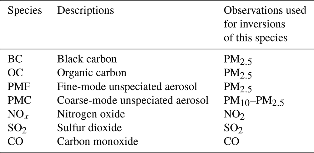
The appropriate estimation of the uncertainty in emissions and chemical concentrations is important for the performance of the inversion estimation using EnKF. Since the source emission data over mainland China in the HTAP_v2.2 inventory are obtained from the MIX inventory (Li et al., 2017b), the uncertainties of emissions of different species, including PMF (fine-mode unspeciated aerosol), PMC (coarse-mode unspeciated aerosol), BC (black carbon), OC (organic carbon), NO_x, CO, SO₂, NH₃ and NMVOCs (non-methane volatile organic compounds), were obtained from Li et al. (2017b) and Streets et al. (2003), which were represented by an ensemble of perturbed emissions generated by multiplying the a priori emissions with a perturbation factor β_i,s:

$$\begin{array}{}\text{(2)}& {\mathit{E}}_{i,s}={\mathit{\beta }}_{i,s}\circ {\mathit{E}}_s^{p}i=\mathrm{1},\mathrm{2},\mathrm{\cdots }{N}_{\mathrm{ens}},\end{array}$$

where E_i,s represents the vector of the ith member of perturbed emissions for species s, ${\mathit{E}}_s^p$ represents the a priori emissions for this species, ∘ denotes the Schur product and N_ens denotes the ensemble size. In this way, the adjustment of emissions is equivalent to the adjustment of perturbation factors.

In terms of the uncertainty in chemical concentrations, considering that emission uncertainty is the major contributor to the uncertainties in air quality modeling, especially during the COVID-19 period when emissions changed rapidly, uncertainties in chemical variables were obtained through ensemble simulations driven by perturbed emissions. The ensemble size was chosen to be 50 to maintain the balance between the filter performance and computational cost. After the ensemble simulations, emissions of multiple species were updated using a deterministic form of EnKF (DEnKF) proposed by Sakov and Oke (2008), which is formulated by

$$\begin{array}{}\text{(3)}& {\displaystyle }\stackrel{\mathrm{‾}}{{\mathit{x}}^{\mathrm{a}}}=\stackrel{\mathrm{‾}}{{\mathit{x}}^{\mathrm{b}}}+{\mathbf{P}}_{\mathrm{e}}^{\mathrm{b}}{\mathbf{H}}^{\mathrm{T}}{\left({\mathbf{HP}}_{\mathrm{e}}^{\mathrm{b}}{\mathbf{H}}^{\mathbf{T}}+\mathbf{R}\right)}^{-\mathrm{1}}\left({\mathit{y}}^{\mathrm{o}}-\mathbf{H}\stackrel{\mathrm{‾}}{x^{\mathrm{b}}}\right),\text{(4)}& {\displaystyle }\stackrel{\mathrm{‾}}{{\mathit{x}}^{\mathrm{b}}}={\displaystyle \frac{\mathrm{1}}{N}}{\sum }_{i=\mathrm{1}}^N{\mathit{x}}_i^{\mathrm{b}};{\mathbf{X}}_i^{\mathrm{b}}={\mathit{x}}_i^{\mathrm{b}}-\stackrel{\mathrm{‾}}{x^{\mathrm{b}}},\text{(5)}& {\displaystyle }{\mathbf{P}}_{\mathrm{e}}^{\mathrm{b}}={\displaystyle \frac{\mathrm{1}}{N-\mathrm{1}}}{\sum }_{i=\mathrm{1}}^N{\mathbf{X}}_i^{\mathrm{b}}{\left({\mathbf{X}}_i^{\mathrm{b}}\right)}^{\mathrm{T}},\end{array}$$

where x denotes the state variables, b the background state (a priori), a the analysis state (posteriori), ${\mathbf{P}}_{\mathrm{e}}^{\mathrm{b}}$ the ensemble-estimated background error covariance matrix and N the ensemble size. y^o represents the vector of observations with an error covariance matrix of R. H is the linear observational operator that maps the m-dimensional state vector x to a p-dimensional (number of observations) observational vector ($\mathbf{H}\stackrel{\mathrm{‾}}{{\mathit{x}}^{\mathrm{b}}}$). The state variables were defined as follows according to the state augmentation method during the assimilation:

$$\begin{array}{}\text{(6)}& {\displaystyle }{\mathit{x}}_i=[{\mathbf{c}}_i,{\mathit{\beta }}_i{]}^T,i=\mathrm{1},\mathrm{2},\mathrm{\cdots }{N}_{\mathrm{ens}},\text{(7)}& {\displaystyle }{\mathit{c}}_i={\left[{\mathrm{PM}}_{\mathrm{2.5}},{\mathrm{PM}}_{\mathrm{10}-\mathrm{2.5}},{\mathrm{NO}}_{\mathrm{2}},{\mathrm{SO}}_{\mathrm{2}},\mathrm{CO}\right]}_i,\text{(8)}& {\displaystyle }{\mathit{\beta }}_i={\left[{\mathit{\beta }}_{\mathrm{PMF}},{\mathit{\beta }}_{\mathrm{BC}},{\mathit{\beta }}_{\mathrm{OC}},{\mathit{\beta }}_{\mathrm{PMC}},{\mathit{\beta }}_{{\mathrm{NO}}_{\mathit{x}}},{\mathit{\beta }}_{{\mathrm{SO}}_{\mathrm{2}}},{\mathit{\beta }}_{\mathrm{CO}}\right]}_i,\end{array}$$

where x_i represents the ith member of the assimilated state variable, which consists of the fields of chemical variables c_i and emission perturbation factors β_i. Detailed descriptions of the model state variables are summarized in Table 1. The use of PM_10−2.5 (PM₁₀ minus PM_2.5) values was aimed at avoiding the potential cross-correlations between PM_2.5 and PM₁₀ (Peng et al., 2018; Ma et al., 2019). Moreover, to prevent spurious correlations between non- or weakly related variables, similar to Ma et al. (2019) and Miyazaki et al. (2012), state variable localization was used during assimilation, with observations of one particular species only used in the updates of the same species' emission rate. The corresponding relationship between the chemical observations and adjusted emissions is summarized in Table 1. The PM_2.5 observations were one exception and were used to update the emissions of PMF, BC and OC since the observations of speciated PM_2.5 were not available in this study. The lack of speciated PM_2.5 observations may lead to uncertainties in the estimated emissions of PMF, BC and OC. Therefore, we only analyzed the emissions of PM_2.5, which were the sum of the emissions of these three species. Similarly, only PM₁₀ emissions were analyzed in this study, which includes the emissions of PM_2.5 and PMC.

Figure 2 Illustration of the iteration inversion scheme used in this study.

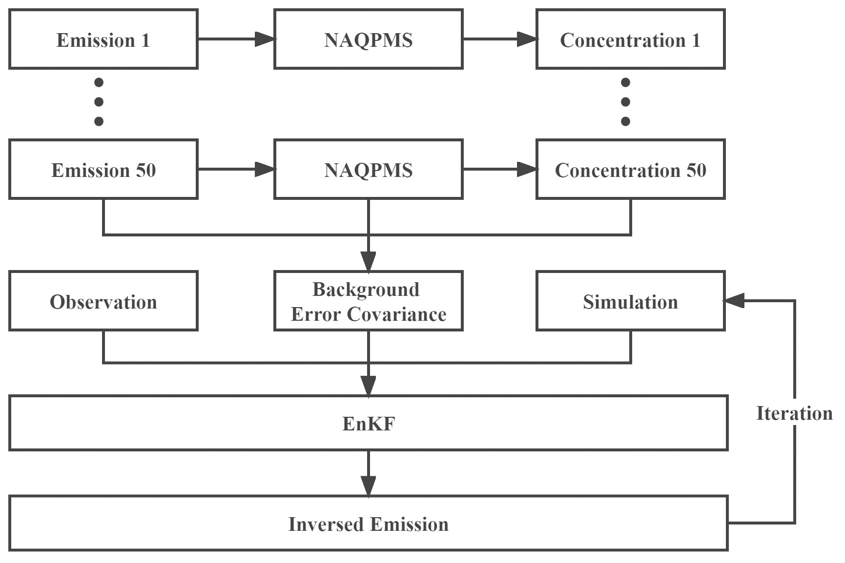
Table 1 Corresponding relationship between the chemical observations and adjusted emissions.

Due to the strict control measures implemented during the last decades, the emissions in China decreased dramatically from 2010 to 2020, especially for SO₂. Thus, there are large biases in the a priori estimates of emissions in China (Zheng et al., 2018), which could lead to incomplete adjustments of the a priori emissions and degrade the performance of the assimilation. Therefore, an iteration inversion scheme was developed in this study to address the large biases of SO₂ emissions. As illustrated in Fig. 2, the main idea of the iteration inversion scheme is to update the ensemble mean of the state variable using the inversion results of the kth iteration and corresponding simulations. The state variable used in the (k+1)th inversions is written as follows:

$$\begin{array}{}\text{(9)}& {\mathit{x}}_i^{k+\mathrm{1}}={\left[{\mathit{c}}^k+{\mathit{c}}_i^{\mathrm{e}}-\stackrel{\mathrm{‾}}{{\mathit{c}}^{\mathrm{e}}},{\mathit{\beta }}^k+{\mathit{\beta }}_i^{\mathrm{e}}-\stackrel{\mathrm{‾}}{{\mathit{\beta }}^{\mathrm{e}}}\right]}^T,\end{array}$$

where c^k represents the simulation results using the inversed emissions of the kth iteration, ${\mathit{c}}_i^{\mathrm{e}}$ represents the ith member of ensemble simulations with an ensemble mean of $\stackrel{\mathrm{‾}}{{\mathit{c}}^{\mathrm{e}}}$, β^k represents the perturbation factors of the kth iteration, and ${\mathit{\beta }}_i^{\mathrm{e}}$ represents the ith member of the ensemble of perturbation factors with a mean value of $\stackrel{\mathrm{‾}}{{\mathit{\beta }}^{\mathrm{e}}}$.

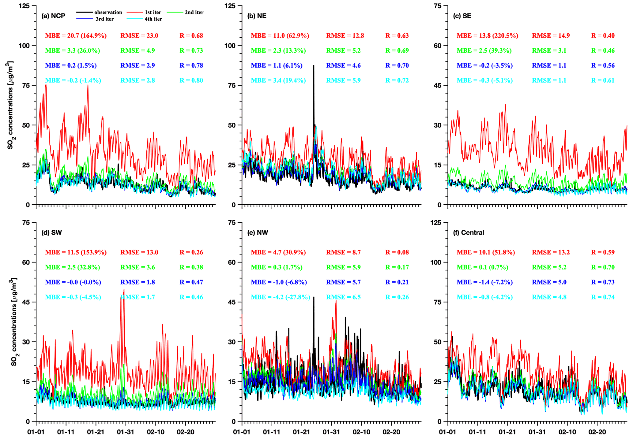
Figure 3 Comparisons of the observed and simulated mean SO₂ concentrations using emissions of different iteration time at validation sites over (a) the NCP region, (b) NE region, (c) SE region, (d) SW region, (e) NW region and (f) central region.

Using this method, the problems of large biases in the a priori emissions were well addressed as exemplified in Fig. 3 for SO₂ emissions. It can be clearly seen that due to the large positive biases in the a priori SO₂ emissions, the model still has large positive biases (normalized mean bias: NMB =30.9 %–220.5 %) and errors (RMSE =8.7–23.0 µg m⁻³) in simulated SO₂ concentration over all regions of China even after assimilation (first iteration). However, the biases and errors continued to decrease with the increase in iteration times till the fourth iteration in which there was no significant improvement in SO₂ simulations compared to those in the third iteration. These results suggested that the iteration inversion method used in this study can constrain well the a priori emissions with large biases and that, in this application, conducting three iterations is enough for constraining the emissions. Besides SO₂ emissions, the iteration inversion scheme was also applied to the emissions of other species. Meanwhile, to reduce the influences of random model errors (e.g., errors in meteorological inputs) on the estimation of the variation in emissions, a 15 d running average was performed on our daily inversion results after the inversion estimation.

Table 2 Configuration of simulation scenarios.

2.4 Quantification of the effects of emission changes and meteorological variations

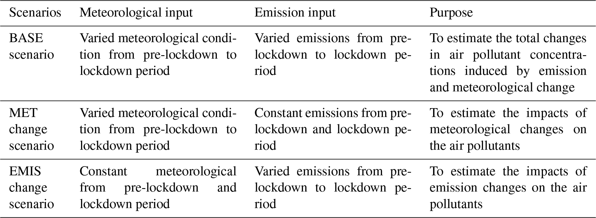
In previous studies, the meteorological-induced (MI) changes were usually determined by the CTM with a fixed emission input setting and a varying meteorological input. Then, the difference between the MI changes and total changes in air pollutant concentrations is defined as emission-induced (EI) changes. Another approach to estimate EI changes is to perform simulations with a fixed meteorological input setting and varying emission inputs. Then, the MI changes are defined as the difference between EI changes and total changes in air pollutant concentrations. Due to the nonlinear effects of atmospheric chemical systems, these two methods yield different results. Thus, both methods were used in this study to account for the nonlinear effects. The averaged results of these two methods are used to represent the impacts of emission changes and meteorological variation on the air quality changes during the COVID-19 restrictions. In total, three scenario experiments were designed based on our inversion results (Table 2). The first scenario simulation used the varying meteorological and emission inputs from the P1 to P2 period, which represents the real-world scenario and is used to estimate the total changes in air pollutant concentrations induced by emissions and meteorological changes from the P1 to P2 period (BASE scenario). The second scenario experiment used the varying meteorological inputs but replaced the emissions during the P2 period with those during the P1 period, which was used to estimate the MI changes using the first method (MET change scenario). The third scenario experiment used the varying emission input and replaced the meteorological input during the P2 period with that during the P1 period, which was used to estimate the EI changes using the second method (EMIS change scenario). Based on the first method, the MI and EI changes can be estimated as follows:

$$\begin{array}{}\text{(10)}& {\displaystyle }\begin{array}{rl}{\mathrm{MI}}_{\text{MET\hspace{0.17em} change\hspace{0.17em} scenario}}& ={\mathrm{conc}}_{\text{p2,\hspace{0.17em} MET\hspace{0.17em} change\hspace{0.17em} scenario }}\\ & -{\mathrm{conc}}_{\text{p1,\hspace{0.17em} MET\hspace{0.17em} change\hspace{0.17em} scenario}}\end{array},\text{(11)}& {\displaystyle }\begin{array}{rl}{\mathrm{EI}}_{\text{MET\hspace{0.17em} change\hspace{0.17em} scenario}}& ={\mathrm{conc}}_{\text{p2,\hspace{0.17em} BASE\hspace{0.17em} scenario}}\\ & -{\mathrm{conc}}_{\text{p1,\hspace{0.17em} BASE\hspace{0.17em} scenario}}\\ & -{\mathrm{MI}}_{\text{MET\hspace{0.17em} change\hspace{0.17em} scenario}}\end{array},\end{array}$$

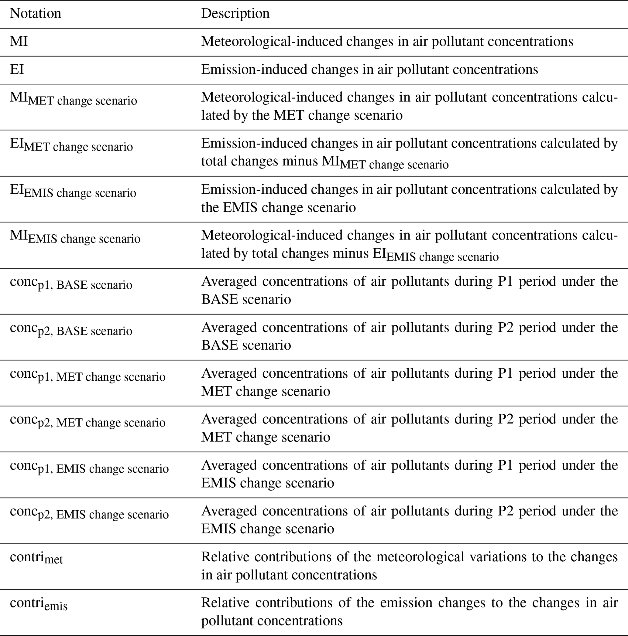
where MI_{MET  change  scenario} represents the MI changes estimated based on the results from the MET change scenario; conc_{p1,  MET  change  scenario} and conc_{p2,  MET  change  scenario} represent the averaged concentrations of air pollutants during the P1 and P2 periods under the MET change scenario; EI_{MET  change  scenario} represents the EI changes estimated based on the results from the MET change scenario; and conc_{p1,  BASE  scenario} and conc_{p2,  BASE  scenario}, respectively, represent the averaged concentrations of air pollutants during the P1 and P2 periods under the BASE scenario. Similarly, the MI and EI changes estimated based on the second method are formulated as follows:

$$\begin{array}{}\text{(12)}& {\displaystyle }\begin{array}{rl}{\mathrm{EI}}_{\text{EMIS\hspace{0.17em} change\hspace{0.17em} scenario}}& ={\mathrm{conc}}_{\text{p2,\hspace{0.17em} EMIS\hspace{0.17em} change\hspace{0.17em} scenario }}\\ & -{\mathrm{conc}}_{\text{p1,\hspace{0.17em} EMIS\hspace{0.17em} change\hspace{0.17em} scenario}}\end{array},\text{(13)}& {\displaystyle }\begin{array}{rl}{\mathrm{MI}}_{\text{EMIS\hspace{0.17em} change\hspace{0.17em} scenario}}& ={\mathrm{conc}}_{\text{p2,\hspace{0.17em} BASE\hspace{0.17em} scenario}}\\ & -{\mathrm{conc}}_{\text{p1,\hspace{0.17em} BASE\hspace{0.17em} scenario}}\\ & -{\mathrm{EI}}_{\text{EMIS\hspace{0.17em} change\hspace{0.17em} scenario}}\end{array},\end{array}$$

Then, the estimations from these two methods are averaged to estimate the contributions of meteorological change and emission change to the changes in PM_2.5 and O₃ concentrations during the COVID-19 lockdown:

$$\begin{array}{}\text{(14)}& {\displaystyle }\mathrm{MI}=({\mathrm{MI}}_{\text{EMIS\hspace{0.17em} change\hspace{0.17em} scenario}}+{\mathrm{MI}}_{\text{MET\hspace{0.17em} change\hspace{0.17em} scenario}})/\mathrm{2},\text{(15)}& {\displaystyle }\mathrm{EI}=({\mathrm{EI}}_{\text{EMIS\hspace{0.17em} change\hspace{0.17em} scenario}}+{\mathrm{EI}}_{\text{MET\hspace{0.17em} change\hspace{0.17em} scenario}})/\mathrm{2},\text{(16)}& {\displaystyle }{\mathrm{contri}}_{\mathrm{met}}={\displaystyle \frac{\mathrm{MI}}{\mathrm{MI}+\mathrm{EI}}}\times \mathrm{100},\text{(17)}& {\displaystyle }{\mathrm{contri}}_{\mathrm{emis}}={\displaystyle \frac{\mathrm{EI}}{\mathrm{MI}+\mathrm{EI}}}\times \mathrm{100},\end{array}$$

where contri_met and contri_emis represent the relative contributions (%) of the meteorological variations and emission changes to the changes in air pollutant concentrations. A detailed definition of each notation used in the calculation of MI and EI changes is given in Table 3.

Table 3 Descriptions of different items used in the calculation of meteorological-induced and emission-induced changes in air pollutant concentrations.

3 Results

3.1 Validation of the inversion results

We firstly validate our inversion system by using a cross-validation method, in which 20 % of observation sites were withheld from the emission inversion and used as the validation datasets. Figures S1–S6 in the Supplement show the concentrations of different air pollutants in China from 1 January to 29 February 2020 obtained from observations at validation sites and simulations using a priori and a posteriori emissions. Commonly used statistical evaluation indices, including correlation coefficient (R), mean bias error (MBE), NMB and root mean square error (RMSE), are summarized in Table S1 in the Supplement. The validation results suggest that the a posteriori simulation agreed well with the observed concentrations for all species. The large biases in the a priori simulation of PM_2.5, PM₁₀, SO₂ and CO were almost completely removed in the a posteriori simulation with NMBs of about −3.9 %–15.7 % for PM_2.5, −3.1 %–11.6 % for PM₁₀, −12.6 %–5.3 % for NO₂, −9.5 %–6.2 % for SO₂ and −10 %–7.6 % for CO (Table S1). RMSE values were also significantly reduced in the a posteriori simulation, which were 9.1–32.2 µg m⁻³ for PM_2.5, 12.6–42.4 µg m⁻³ for PM₁₀, 5.1–12.3 µg m⁻³ for NO₂, 1.2–5.6 µg m⁻³ for SO₂ and 0.10–0.46 mg m⁻³ for CO. Moreover, the inversion emissions considerably improved the fit to the observed time evolution of air pollutants' concentrations. The R values were improved for all species in the a posteriori simulation, which were up to 0.74–0.94 for PM_2.5, 0.63–0.92 for PM₁₀, 0.76–0.94 for NO₂, 0.23–0.79 for SO₂ and 0.63–0.92 for CO. These results suggest that our inversion results have excellent performance in representing the magnitude and variation in these species' emissions in China during COVID-19 restrictions. Model performance in simulating O₃ concentrations is relatively poor compared to other species although improvement was remarkable in the NCP, NE and SW regions. This would be due to the use of an outdated emission inventory for the base year of 2010 and that the emissions of non-mental volatile organic compounds (NMVOCs), another important precursor for O₃, were not constrained in this study. As shown in Fig. S7, the NMVOC emissions for the base year of 2010 were generally lower than those for 2018 except over the SW regions. Considering the increasing trend of NMVOC emissions in China (Li et al., 2019), the underestimates of NMVOC emissions for the base year of 2020 could be larger. This is in line with the negative biases in the simulated O₃ concentrations over these regions.

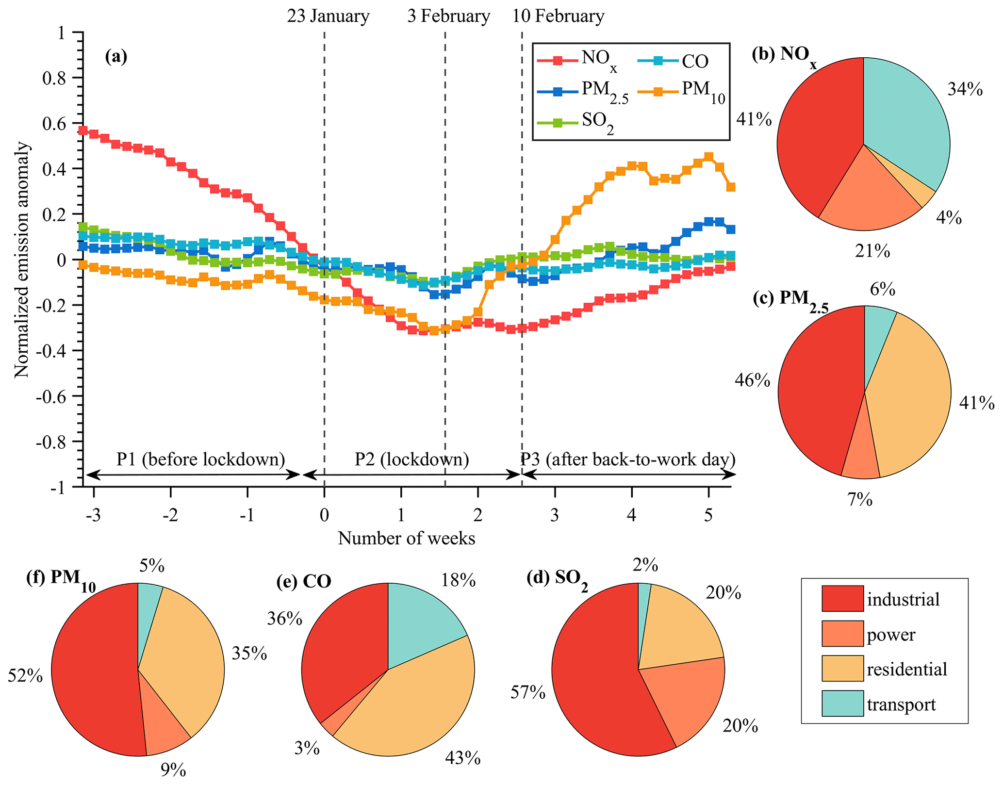
Figure 4 (a) Time series of normalized emission anomalies estimated by inversion results for different species in China from 1 January to 29 February 2020 and (b–f) relative contributions of different sectors to the total anthropogenic emissions of NO_x, PM_2.5, PM₁₀, CO and SO₂ obtained from Zheng et al. (2018). The normalized emission anomaly is calculated by the emission anomaly divided by the average emissions during the whole period.

3.2 Emission changes in multiple species during COVID-19 restrictions

3.2.1 Unbalanced emission changes between NO_x and other species

The control of COVID-19 began on 23 January 2020 when the Chinese government declared the first level of national responses to public health emergencies, 1 d before Chinese New Year's Eve. Figure 4 shows the time evolution of the normalized emission anomaly for different species in China from 1 January to 29 February. The temporal variation in the emissions varied largely between NOx and other species. Due to the combined effects of the Spring Festival and COVID-19 lockdown, NO_x emissions decreased continuously at the beginning of January until approximately 1 week after the implementation of the COVID-19 lockdown, with estimated decreases in NO_x emissions of up to 42.5 % from the P1 to P2 period (Table 4). Subsequently, the NO_x emissions stabilized with small fluctuations until the official back-to-work day when the NO_x emissions began to increase due to the easing of the control measures and the resumption of business. According to inversion estimation, NO_x emissions recovered by 3.9 % during the P3 period. These results indicate that the temporal variation in our estimated NO_x emissions agreed well with the timing of the Spring Festival and different control stages of COVID-19. However, for other species (i.e., PM_2.5, PM₁₀, SO₂ and CO), although their emissions generally decreased from 1 January to the end of the 2020 Spring Festival holiday, they showed much smaller reductions than the NO_x emissions. The emission reduction for these species was only approximately 7.9 %–12.1 % (Table 4). This is consistent with the inversion results of Hu et al. (2022), who found that SO₂ emissions in China decreased only by 9.2 % during the COVID-19 lockdown. In addition, the emissions of these species quickly rebounded to their normal level just 1 week after the end of the Spring Festival holiday. As estimated by our inversion results, the SO₂ emissions recovered by 7.2 % during the P3 period, which was only 2.5 % lower than that during the P1 period. The PM_2.5 and PM₁₀ emissions during the P3 period were 3.3 % and 43.6 % higher, respectively, than those during the P1 period.

Table 4 Inversion estimated emissions of different air pollutants in China and their changes between different periods during COVID-19.

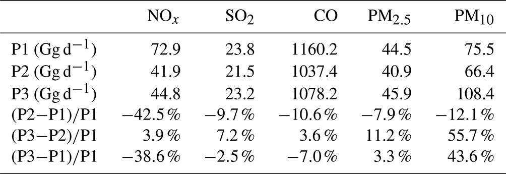
Table 5 Inversion estimated emission changes of different air pollutants over different regions in China between different periods during COVID-19 restrictions.

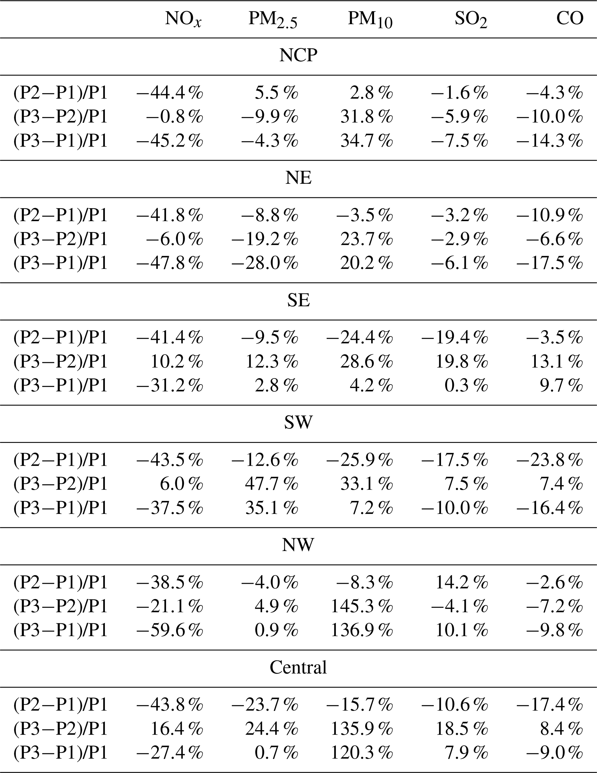
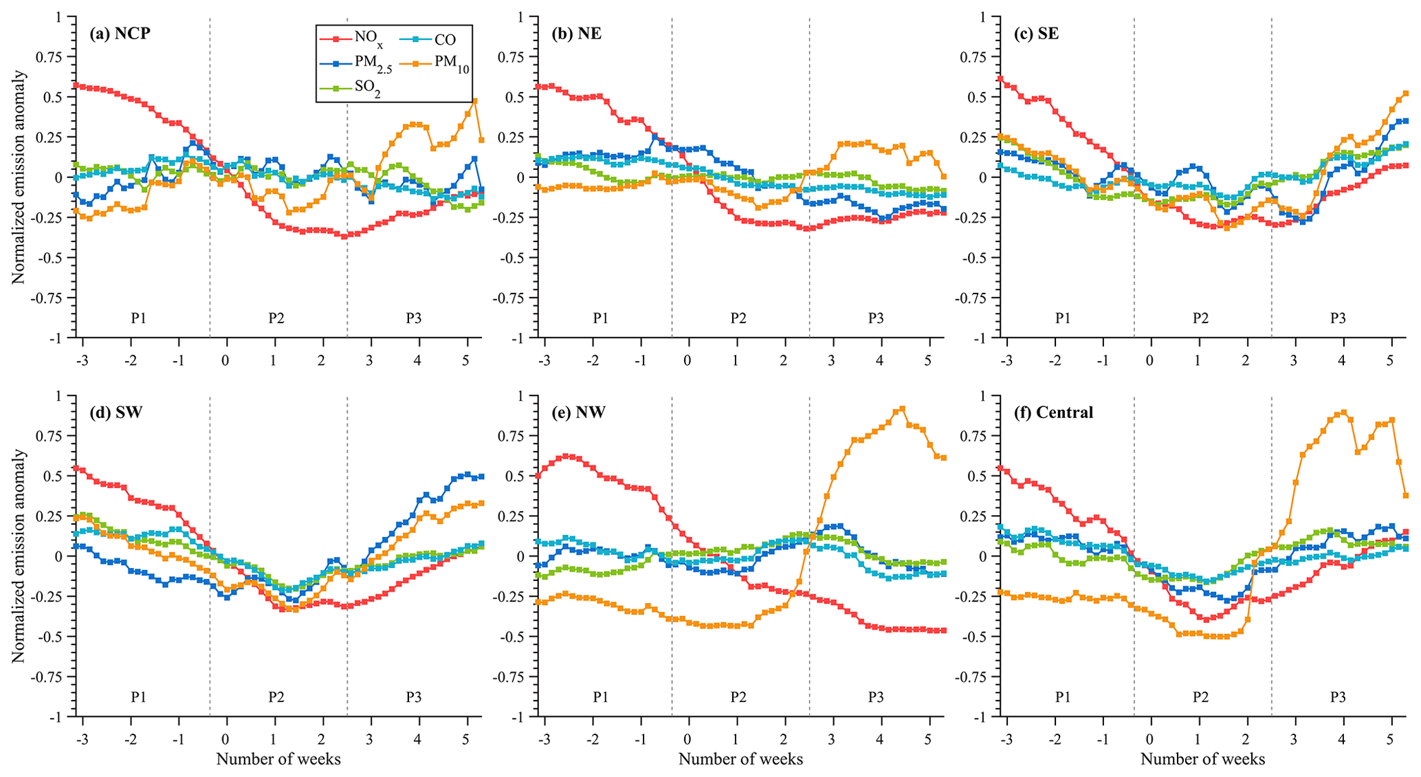
Figure 5 Time series of normalized emission anomalies estimated by inversion results for different species over (a) the NCP region, (b) NE region, (c) SE region, (d) SW region, (e) NW region and (f) central region from 1 January to 29 February 2020.

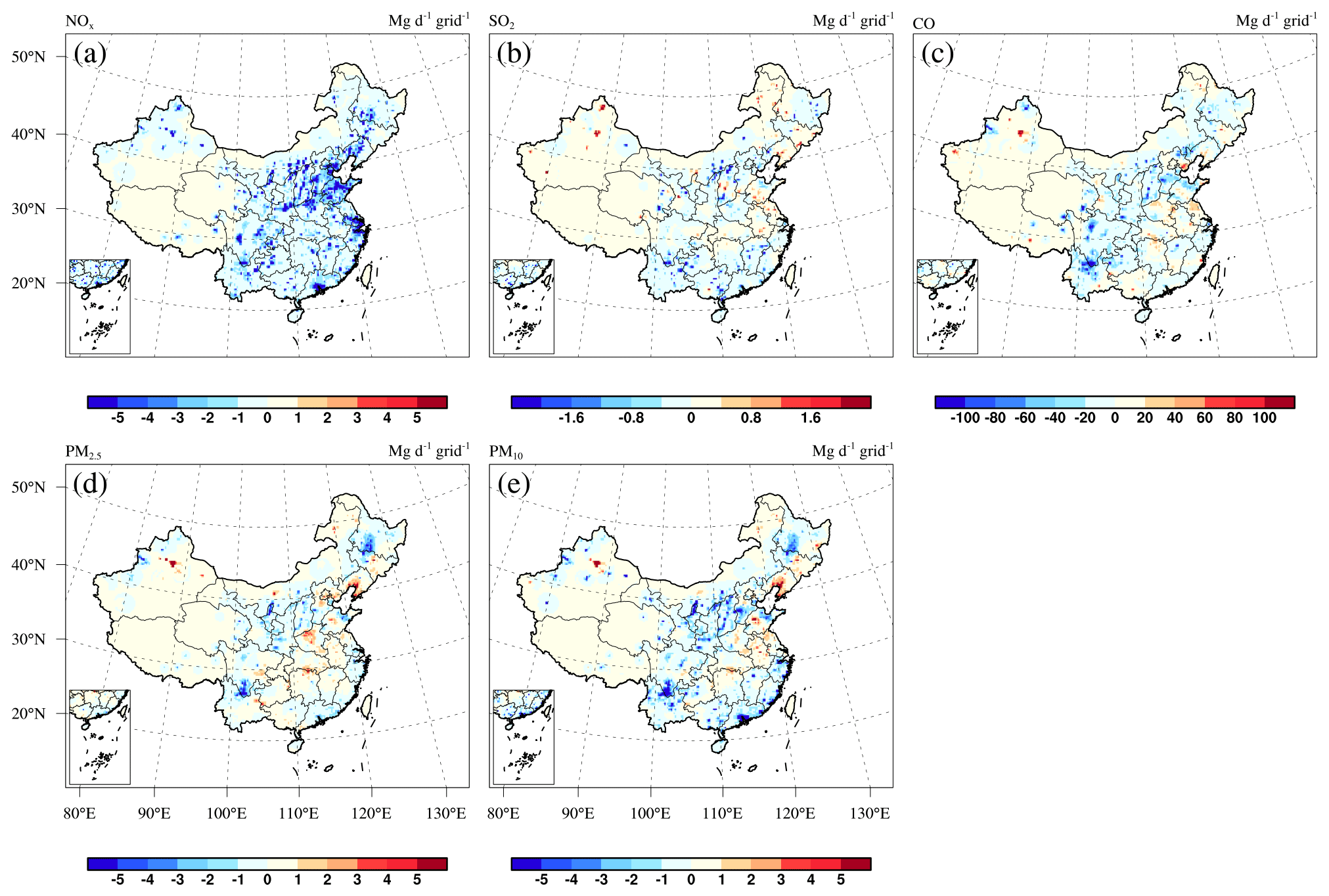
Figure 6 The inversion estimated emission changes in (a) NO_x, (b) SO₂, (c) CO, (d) PM_2.5 and (e) PM₁₀ in China from P1 to P2 period.

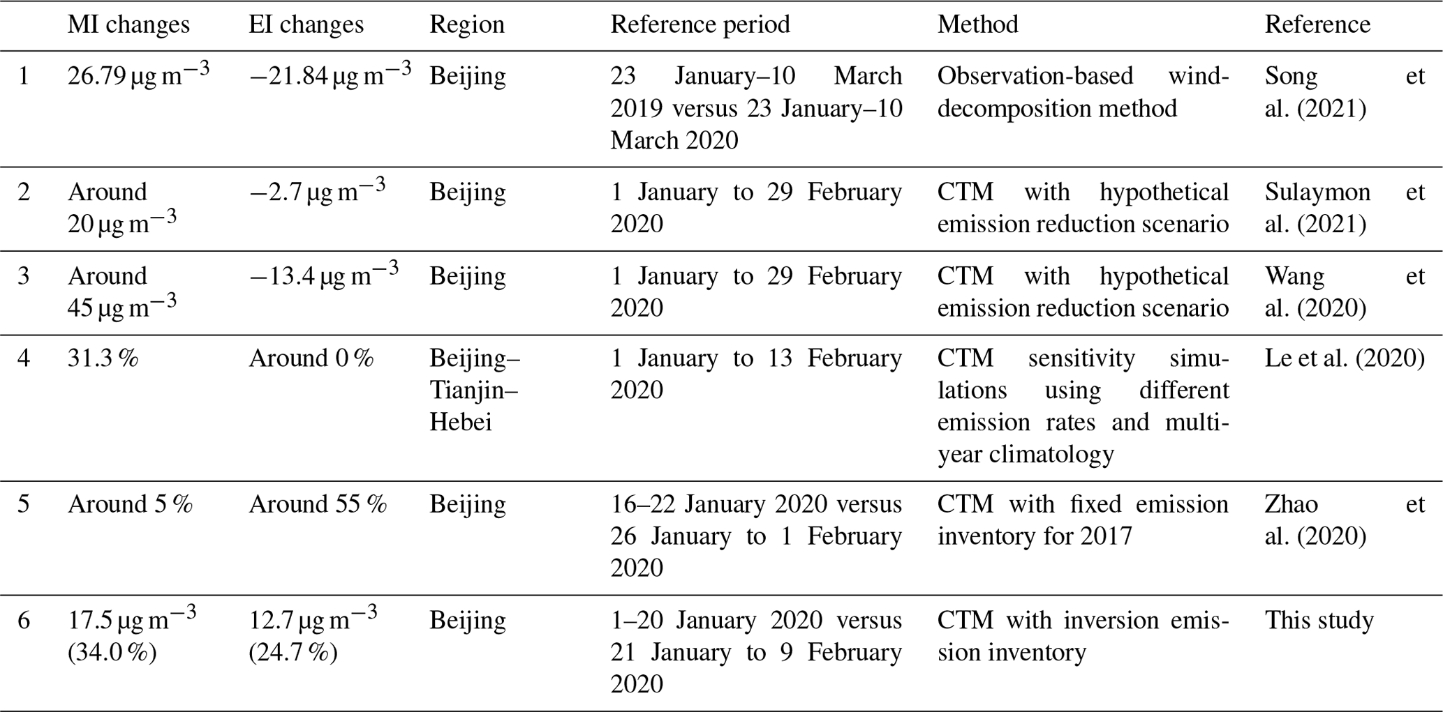
Table 6 Calculated MI and EI changes in PM_2.5 concentrations during the COVID-19 pandemic by previous studies.

Similar results were found in different regions of China (Fig. 5 and Table 5), where the NO_x emissions decreased much more than other species. In addition, unlike the uniform decreases in NO_x emissions in different regions of China (∼40 %), there was apparent spatial heterogeneity in the emission changes of PM_2.5, PM₁₀, SO₂ and CO (Table 5 and Fig. 6). For example, from the P1 to P2 period, the PM_2.5 emissions decreased by over 20 % in the central region but only by 8.8 % in the NE region. The PM_2.5 emissions even increased by 5.5 % in the NCP region. This may be due to the increased emissions from industry and fireworks according to the field measurements conducted by previous studies (Li et al., 2022; Ma et al., 2022; Zuo et al., 2022; Dai et al., 2020). Based on the measurement of stable Cu and Si isotopic signatures and distinctive metal ratios in Beijing and Hebei, Zuo et al. (2022) analyzed the variations in the PM_2.5 sources during the COVID-19 pandemic, who reported that the primary PM_2.5 emissions did not decrease in Beijing and Hebei and that the PM-associated industrial emissions may have actually increased during the lockdown period. The increased industrial heat sources detected by Li et al. (2022) based on VIIRS (Visible Infrared. Imaging Radiometer Suite) active fire data also supported the increased industrial emissions over the NCP region during the lockdown period. Meanwhile, consistent with the field measurements in Beijing and Tianjin conducted by Ma et al. (2022) and Dai et al. (2020), substantially high levels of potassium (K⁺) and magnesium (Mg²⁺) ions were found over the NCP region during the Spring Festival according to the aerosol chemical composition measurements obtained from CNEMC (Fig. S8). Since K⁺ and Mg²⁺ are two important fingerprints of the firework emissions, the high levels of K⁺ and Mg²⁺ suggest that the emissions from fireworks during the Spring Festival were also a potential contributor to the increase in PM_2.5 emissions over the NCP region. In contrast, the SW and central regions exhibited relatively larger emission reductions for these species (Fig. 5 and Table 5) by 12.6 %–25.9 % and 10.6 %–23.7 %, respectively. The emission rebound during the P3 period was more prominent in the SE, central and SW regions (Figs. 5 and 7), where emissions recovered by 6.0 %–16.4 % for NO_x, 7.5 %–19.8 % for SO₂, 7.4 %–13.1 % for CO, 12.3 %–47.7 % for PM_2.5 and 28.6 %–135.9 % for PM₁₀ (Table 5). This result is consistent with the earlier degradation of the response level to the COVID-19 virus (from the first level to the second or third level) over these regions (Table S2). In contrast, there were decreases in emissions in the NCP, NE and NW regions. PM_2.5 emissions were reduced by 9.9 % in the NCP region and by 19.2 % in the NE region from the P2 to P3 period (Table 5). Moreover, we found that the PM₁₀ emissions surged in the NW and central regions, where the PM₁₀ emissions during the P3 period were almost 2 times higher than those during the P2 period (Table 5). However, this finding may be related to the enhanced dust emissions over these two regions rather than the effects of returning to work according to the decreased PM_2.5 $/$ PM₁₀ ratios during the P3 period. According to Fig.S9, the PM_2.5 $/$ PM₁₀ ratio was relatively stable during the P1 and P2 period, but it decreased substantially during the P3 period, from 0.81 to 0.48 over the NW region and from 0.77 to 0.53 over the central region. A lower PM_2.5 $/$ PM₁₀ ratio commonly suggests that the PM₁₀ is more likely to be attributed to natural sources such as dust (Wang et al., 2015; Fan et al., 2021). Moreover, the NW and central region are typical source areas of dust in China, therefore the increasing PM₁₀ emissions over the NW and central regions may be mainly related to the enhanced dust emissions. This demonstrates the necessity of considering changes in natural emissions during COVID-19 restrictions. Thus, to reduce the effects of natural emissions on our findings, the same analysis was performed for the emissions over southeast China (Fig. S10) where emissions were dominated by anthropogenic sources, which shows consistent results with the findings above (Fig. S11 and Table S3).

3.2.2 Explanations for the emission changes during COVID-19 restrictions

Two explanations may help clarify the unbalanced emission changes between NO_x and other species. First, the COVID-19 lockdown policy has led to dramatic decreases in transportation activities throughout China; however, as shown in Fig. 4, the relative contributions of the transportation sector to the emissions of SO₂ (2.4 %), CO (18.5 %), PM_2.5 (6.1 %) and PM₁₀ (4.7 %) are much smaller than those for NO_x emissions (34.3 %) (Zheng et al., 2018; Li et al., 2017a). Thus, the reduction in traffic activities can only substantially decrease NO_x emissions. Reductions of CO emissions (−10.6 %) were relatively larger than those for SO₂ (−9.7 %) and PM_2.5 (−7.9 %) emissions, which is consistent with the relatively larger contributions of the transportation sector to CO emissions. However, the differences in the percentage decreases in emissions of CO, SO₂ and PM_2.5 are not as significant as the differences in their transportation share (18 % versus 2 % and 6 %). This may be, on the one hand, due to the uncertainty in the estimated relative contributions of different sectors to the total emissions of CO, SO₂ and PM_2.5, but, on the other hand, they were possibly due to the uncertainty in the emission inversions, especially considering that the decreasing trend of CO, SO₂ and PM_2.5 was not significant. Also, other factors beyond transportation may have influenced the reductions of anthropogenic emissions during the P2 period. For example, the PM₁₀ emissions showed the largest reductions among these four species, which is related in part to the reduced dust emissions due to shutting down of construction sites during the lockdown period (Li et al., 2020). Second, as shown in Fig. 4, the industrial and residential sectors are the major contributors to the anthropogenic emissions of SO₂, CO, PM_2.5 and PM₁₀ in China, together contributing 77.6 %, 78.3 %, 86.5 % and 86.3 %, respectively, to their total emissions. The much smaller reductions of these species' emissions were thus in line with the fact that there were no intentional restrictions on heavy industry during the COVID-19 restrictions. A large number of non-interruptible processes, such as steel, glass, coke, refractory, petrochemical, electric power, and especially heating, could not be stopped during the COVID-19 lockdown. According to statistical data from the National Bureau of Statistics of China (Fig. S12), the industrial and power sectors did not show similar reductions of their activity levels as those seen in the transportation sector. Power generation and steel production even showed increases in many provinces, which corresponds well with the emission increases over these regions. In addition, since people were required to stay at home, residential emissions were likely increased due to the increased energy consumption for heating or cooking. Therefore, our inversion results supported the views that the emissions of species related to industrial and residential activities did not decline much during the lockdown period and that the COVID-19 lockdown policy was largely a traffic control measure with small influences on other sectors.

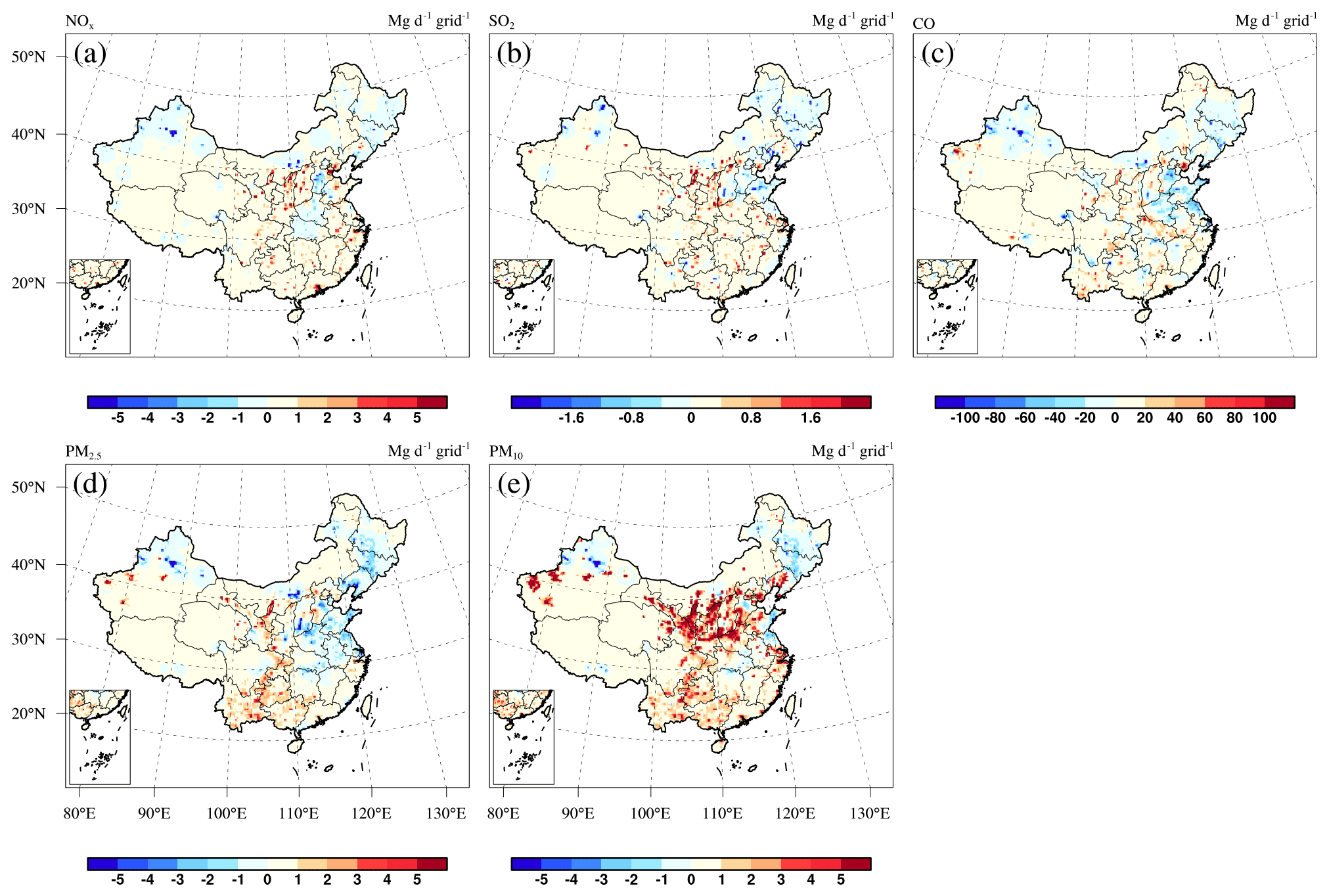
Figure 7 The inversion estimated emission changes in (a) NO_x, (b) SO₂, (c) CO, (d) PM_2.5 and (e) PM₁₀ in China from P2 to P3 period.

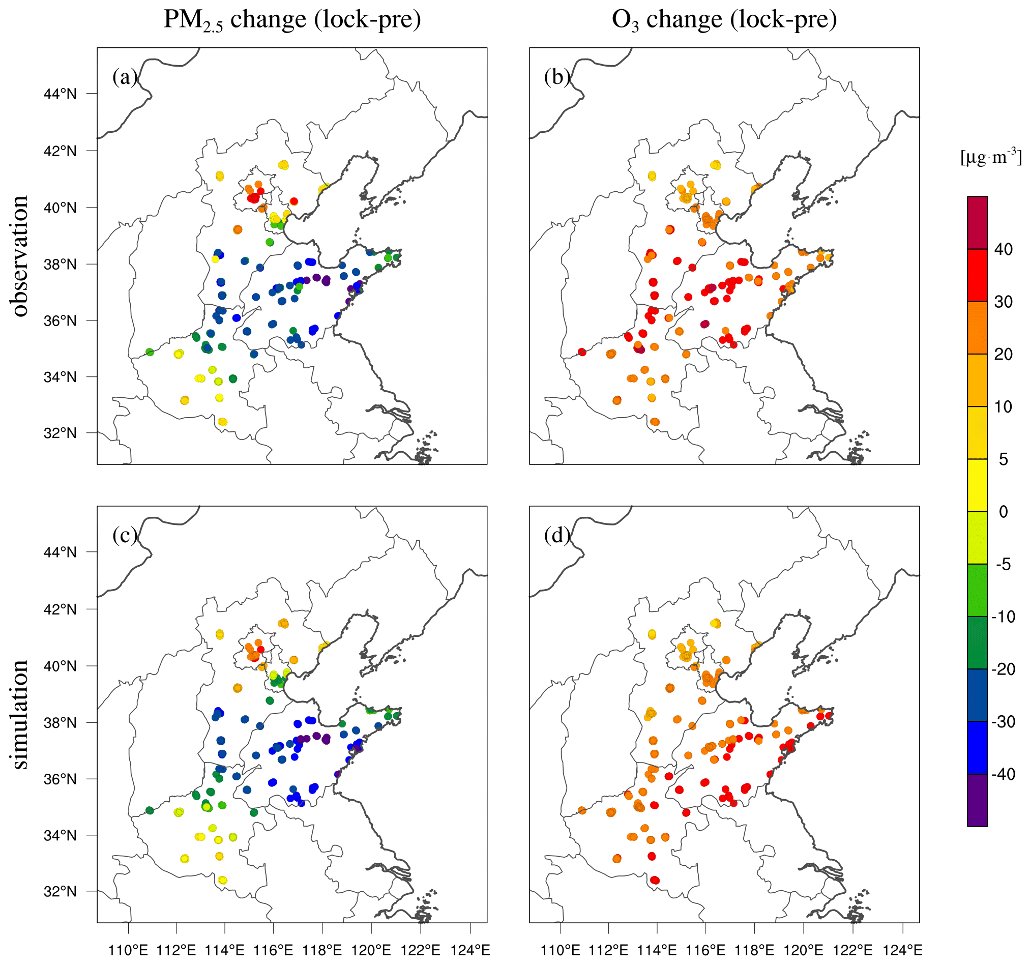
Figure 8 Changes in the observed and simulated concentrations of (a, c) PM_2.5 and (b, d) O₃ over the NCP region from the pre-lockdown period (P1) to the lockdown period (P2).

3.3 Investigation of air quality change over the NCP region during COVID-19 restrictions

Using the inversion results, we reassessed the environmental impacts of the COVID-19 restrictions on the air pollution over the NCP region. The NCP region was chosen because it is the key target region of air pollution control in China and where unexpected severe haze occurred. A major caveat in previous studies that explored the impacts of COVID-19 lockdowns on air quality is the uncertainty in the emission changes during COVID-19 restrictions. The inversion results enable us to give a more reliable assessment of the environmental impacts of COVID-19 restrictions. Figure 8 shows the observed changes in PM_2.5 and O₃ concentrations over the NCP region from the P1 to P2 period. The observations showed consistent reductions of PM_2.5 concentrations over the NCP region (by 13.6 µg m⁻³). However, substantial increases in PM_2.5 concentrations were observed in the Beijing area (by 31.2 µg m⁻³). In contrast to the widespread reductions of PM_2.5 concentrations, the O₃ concentrations significantly increased over the whole NCP region (by 28.3 µg m⁻³) and the Beijing area (by 16.8 µg m⁻³). The simulations based on our inversion results reproduced the observed changes in PM_2.5 and O₃ concentrations over the NCP region well, although the O₃ concentrations were underestimated in all regions (Fig. S6) and the changes in PM_2.5 and O₃ concentrations were slightly overestimated by 1.6 and 2.6 µg m⁻³ in the simulation (Fig. 8).

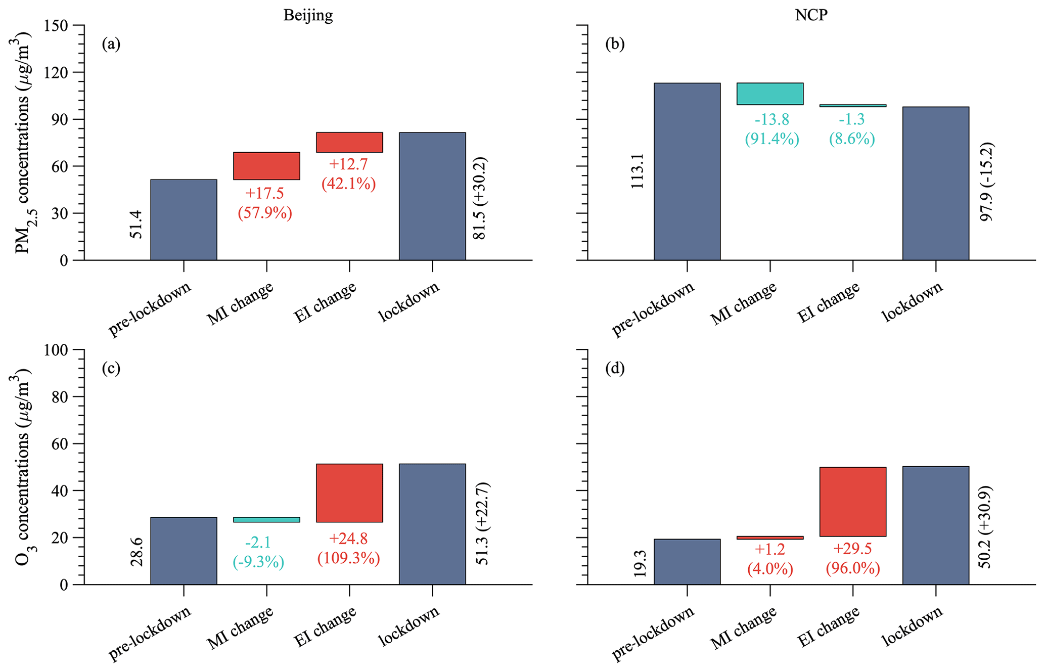
Figure 9 Contributions of the meteorological variations and emission changes to the changes in (a, b) PM_2.5 and (c, d) O₃ concentrations over Beijing and the NCP region from the pre-lockdown period (P1) to the lockdown period (P2).

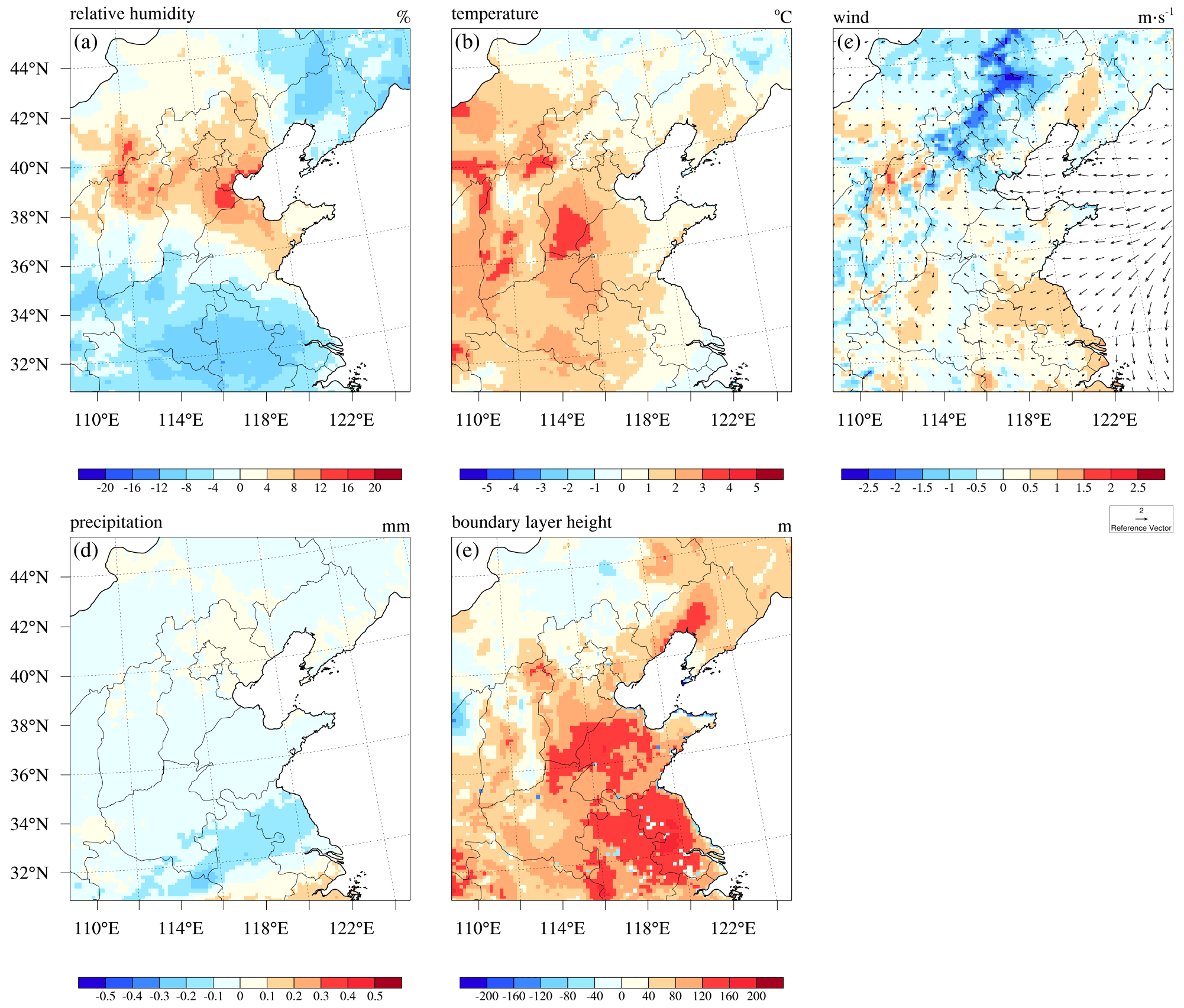
Figure 10 Changes in the (a) relative humidity, (b) temperature, (c) wind speed, (d) precipitation and (e) boundary layer height over the NCP region from P1 to P2 period obtained from WRF simulations.

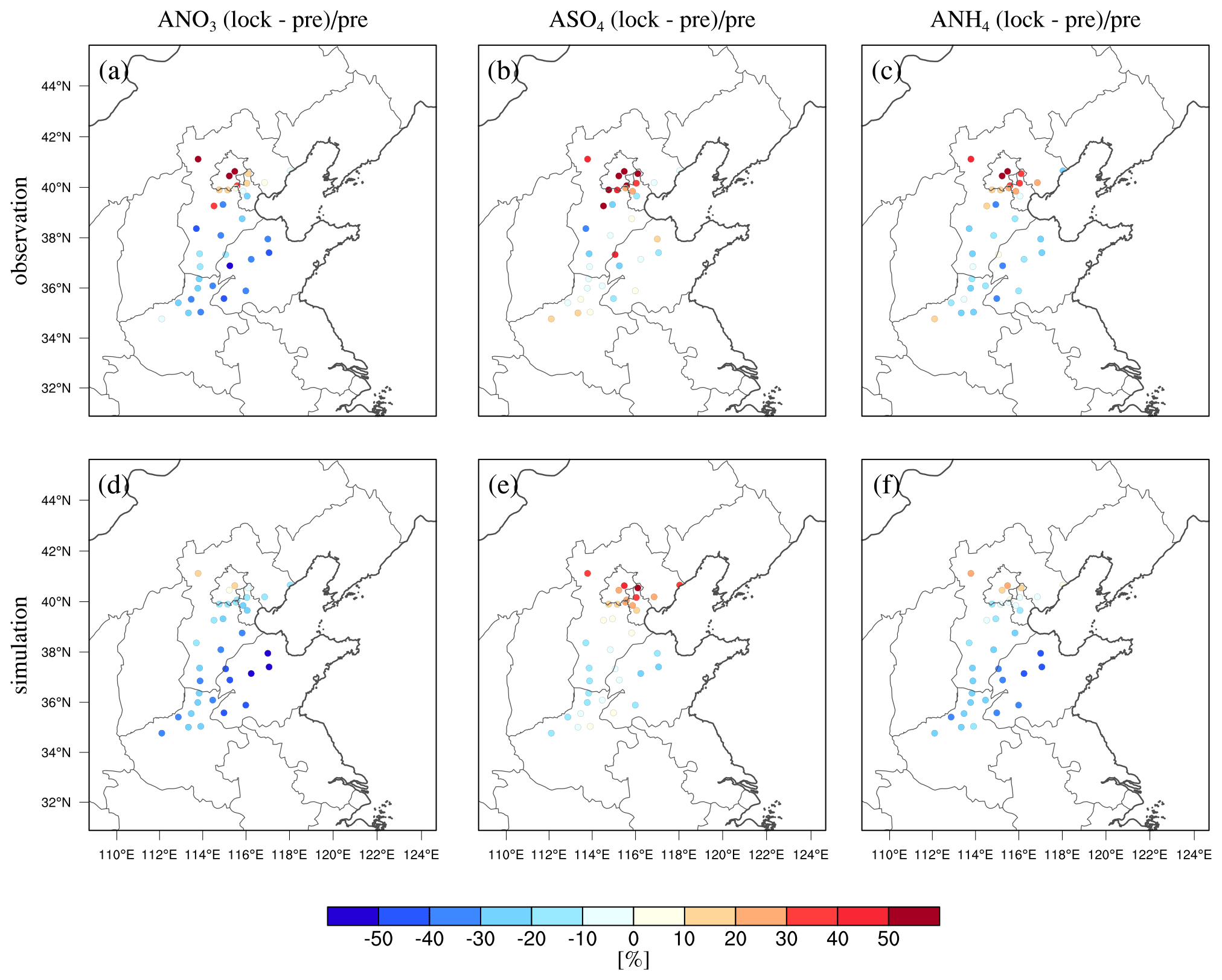
Figure 11 Relative changes in the simulated and observed concentrations of (a, d) ANO₃, (b, e) ASO₄, (c, f) ANH₄ over the NCP region from P1 to P2 period.

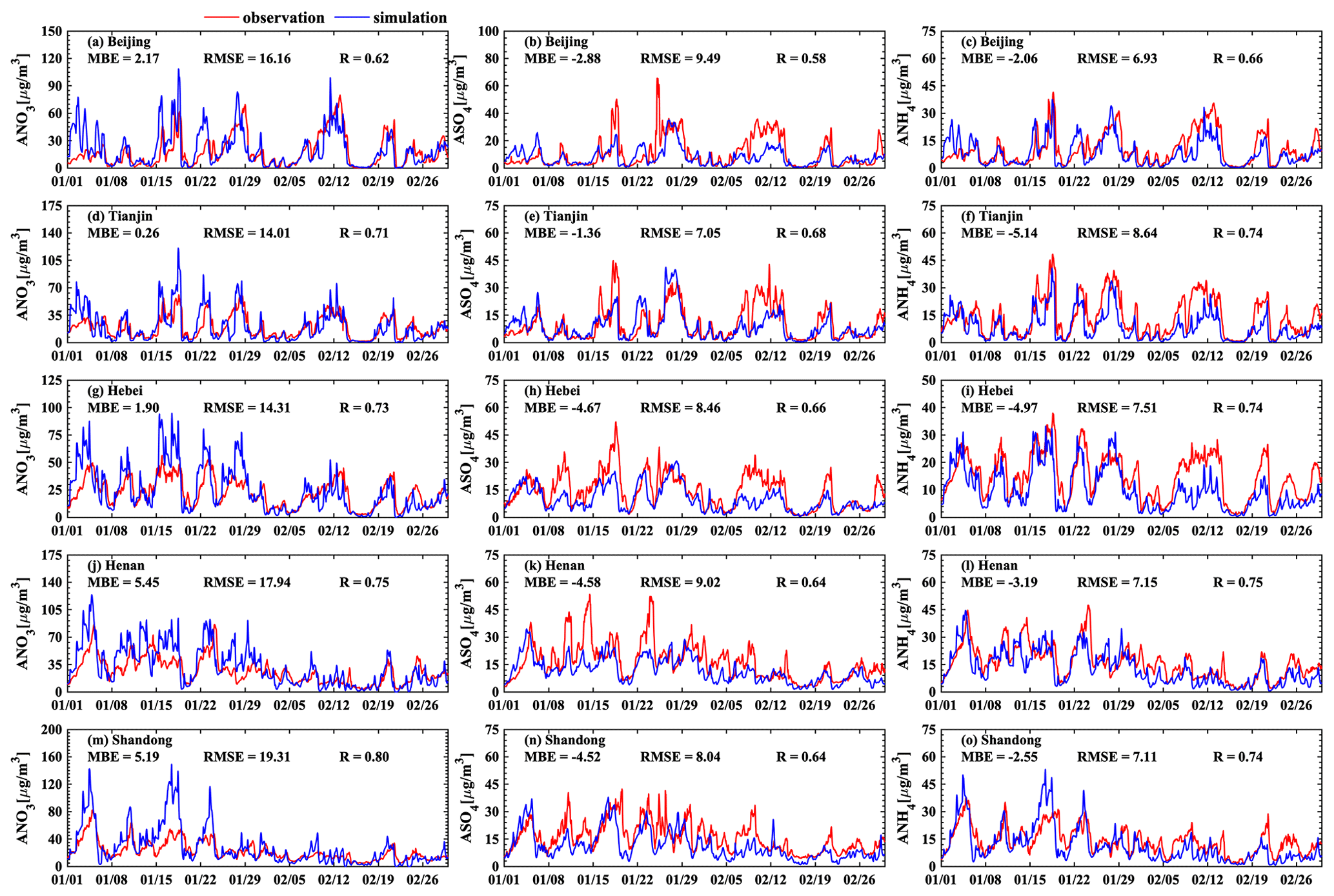
Figure 12 Time series of observed and simulated concentrations of ANO₃, ASO₄ and ANH₄ in (a–c) Beijing, (b–f) Tianjin, and (g–i) Heibei, (j–l) Henan and (m–o) Shangdong provinces from 1 January to 29 February 2020.

As detailed in the Sect. 2.4, the simulated changes in air pollutant concentrations before and after lockdown were decomposed into meteorological-induced (MI) changes and emission-induced (EI) changes through two different scenarios to account for the nonlinearity of the atmospheric chemical system. According to Fig. S13, the differences in calculated MI and EI changes based on different scenarios were small for PM_2.5 concentrations, which were about 2 µg m⁻³ in this application, while they were relatively larger for O₃, which were around 5 µg m⁻³ over the Beijing and NCP region (Fig. S14). In addition, the sign of calculated MI changes using different scenarios was opposite, although both suggested weak contributions of meteorological variation to the changes in O₃ concentrations. This suggests that the calculated MI and EI changes in O₃ concentrations could be more sensitive to the scenarios used, which may be associated with the stronger chemical nonlinearity of the O₃ concentrations. Figure 9 shows the mean results of the calculated MI and EI changes using the two different scenarios. It shows that the meteorological variation dominated the changes in PM_2.5 concentrations over the NCP region, which contributed 90 % of the PM_2.5 reductions over most parts of the NCP region. Moreover, this variation made significant contributions (57.9 %) to the increases in PM_2.5 concentrations over the Beijing area. This finding suggested that meteorological variations played an irreplaceable role in the occurrence of the unexpected PM_2.5 pollution around the Beijing area. Compared with the meteorological conditions before lockdown (Fig. 10), there were increases in relative humidity over northern China, which facilitated the reactions for aerosol formation and growth. Wind speed also decreased over the Beijing area accompanied by an anomalous south wind, which facilitated aerosol accumulation and the transportation of air pollutants from the polluted industrial regions of Hebei Province to Beijing. The increases in boundary layer height from the P1 to P2 period were also much smaller in the Beijing area than in other areas of the NCP. Thus, the Beijing area has exhibited distinct meteorological variations from other areas of the NCP region, which correspond well to the different changes in PM_2.5 concentrations over the Beijing area.

The emission changes contributed slightly to the PM_2.5 reductions over the NCP region (8.6 %). This is because, on the one hand, the large reductions of NO_x emissions (by 44.4 %) only reduced nitrate by approximately 10 %–30 % due to the nonlinear effects of chemical reactions (Fig. 11), and, on the other hand, the emissions of primary PM_2.5 and its precursors from other sectors changed little during the COVID-19 restrictions (Table 5). The emission changes contributed more to the increased PM_2.5 concentrations over the Beijing area (42.1 %). This is mainly associated with the increases in primary PM_2.5 emissions around the Beijing area, as seen in Fig. 6, possibly due to the increased emissions from the different industries as we mentioned before (Zuo et al., 2022) and the increased firework emissions during the Spring Festival as shown by the rapid increases in concentrations of K⁺ and Mg²⁺ measured by CNEMC (Fig. S15). Therefore, our results suggested that the unexpected PM_2.5 pollution during the lockdown period was mainly driven by unfavorable meteorological conditions, together with small changes or even increases in primary PM_2.5 emissions. This finding is in line with previous results of Le et al. (2020) but different from those of Huang et al. (2021), who suggested that enhanced secondary aerosol formation was the main driver of severe haze during the COVID-19 restrictions. To investigate it, we further analyzed the changes in the concentrations of secondary inorganic aerosols (SIAs). First, we evaluated our model results against the observed SIA concentrations, which showed that the model results using our inversion emissions reproduced well the observed concentrations of SIAs over the NCP region (Fig. 12) with mean bias (MB) ranging from −5.14 to 5.45 µg m⁻³ and correlation coefficient (R) ranging from 0.59 to 0.80. The observed increases in SIA concentrations over the Beijing area, especially for sulfate concentrations, were also captured in our simulations (Fig. 11), although underestimation occurred due to the uncertainty in simulating SIA concentrations. Through sensitivity experiments, we found that the increases in SIA concentrations were still driven by meteorological variations (Fig. 13). In fact, the emission reductions only led to a 10 % decrease in SIA concentrations over the NCP region. This finding suggests that the enhanced secondary aerosol formation was likely mainly driven by the unfavorable meteorological conditions associated with higher temperature and relative humidity instead of the emission reductions during the lockdown period. This is in line with the observation evidence from Ma et al. (2022), who emphasized that the increased temperature and relative humidity promoted the formation of secondary pollutants during the COVID-19 restrictions.

In terms of O₃ concentrations, the emission changes subsequently became the dominant contributor to the O₃ increases by more than 100 % in the Beijing area and by 96.0 % over the NCP region. This result is mainly because the lockdown period occurred in midwinter when photochemical O₃ formation was minimal; thus, the large increase in O₃ is expected solely from the effect of the reduced titration reaction associated with the large reductions of NO_x emissions. Although the higher temperature and slower wind speed during the lockdown period were favorable for the increases in O₃ concentrations, their contributions were much smaller than those of emission changes (Fig. 9). These results suggested that control measures, such as COVID-19 restrictions, were inefficient for air pollution mitigation in China considering the high economic cost of the COVID-19 restrictions.

We also compared our results with previous studies that differentiated between the contributions of meteorology and emissions to the PM_2.5 and O₃ concentrations. Before comparisons, it should be noted that it is difficult to directly compare our results with previous studies due to the altered definition of the meteorological contribution, different reference period that was used to quantify the meteorological contributions and different targeted region. For example, in Song et al. (2021), the reference period used to determine the meteorological contribution is the corresponding period of the COVID-19 pandemic in 2019. Le et al. (2020) used the multiyear climatology as the reference period. In Wang et al. (2020) and Sulaymon et al. (2021), the MI changes in PM_2.5 concentrations were defined as the difference between the modeled concentrations on high-pollution days and those on low-pollution days in hypothetical emission reduction scenarios. Zhao et al. (2020) used a similar reference period to ours to determine the MI changes, but they used the outdated emission inventory. Table 6 summarized the results from the selected studies over Beijing and the Beijing–Tianjin–Hebei region. Note that some studies only provided the relative changes in the modeled PM_2.5 concentrations. It shows that due to the uncertainties in emission changes during the COVID-19 pandemic, the EI changes estimated by Zhao et al. (2020) were possibly overestimated compared to our studies (55 % versus 24.7 %). Both Sulaymon et al. (2021) and Wang et al. (2020) suggested negative EI changes during the COVID-19 period in Beijing. This because they presumed that the emissions were largely reduced during the COVID-19 lockdown which may deviate from the real changes in emissions according to our inversion results. Meanwhile, although they used the same method and reference period, their results differed largely (−2.7 versus −13.4 µg m⁻³) due to the different emission reduction scenario they assumed. Le et al. (2020) only considered the emission reductions of NO_x in their sensitivity simulations without considerations of other species; therefore their calculated EI changes may be underestimated compared to our results (almost 0 % versus 24.7 %). However, the calculated MI changes were consistent between our study and Le et al. (2020). In terms of O₃, the calculated EI changes by our study were also higher than those calculated by Zhao et al. (2020) in Beijing (85.7 % versus 70 %). These results suggested that the EI and MI changes calculated by our study could be more reasonable, considering that the emissions of different species were well constrained, which could better represent the temporal variation and spatial heterogeneity of emission changes during COVID-19.

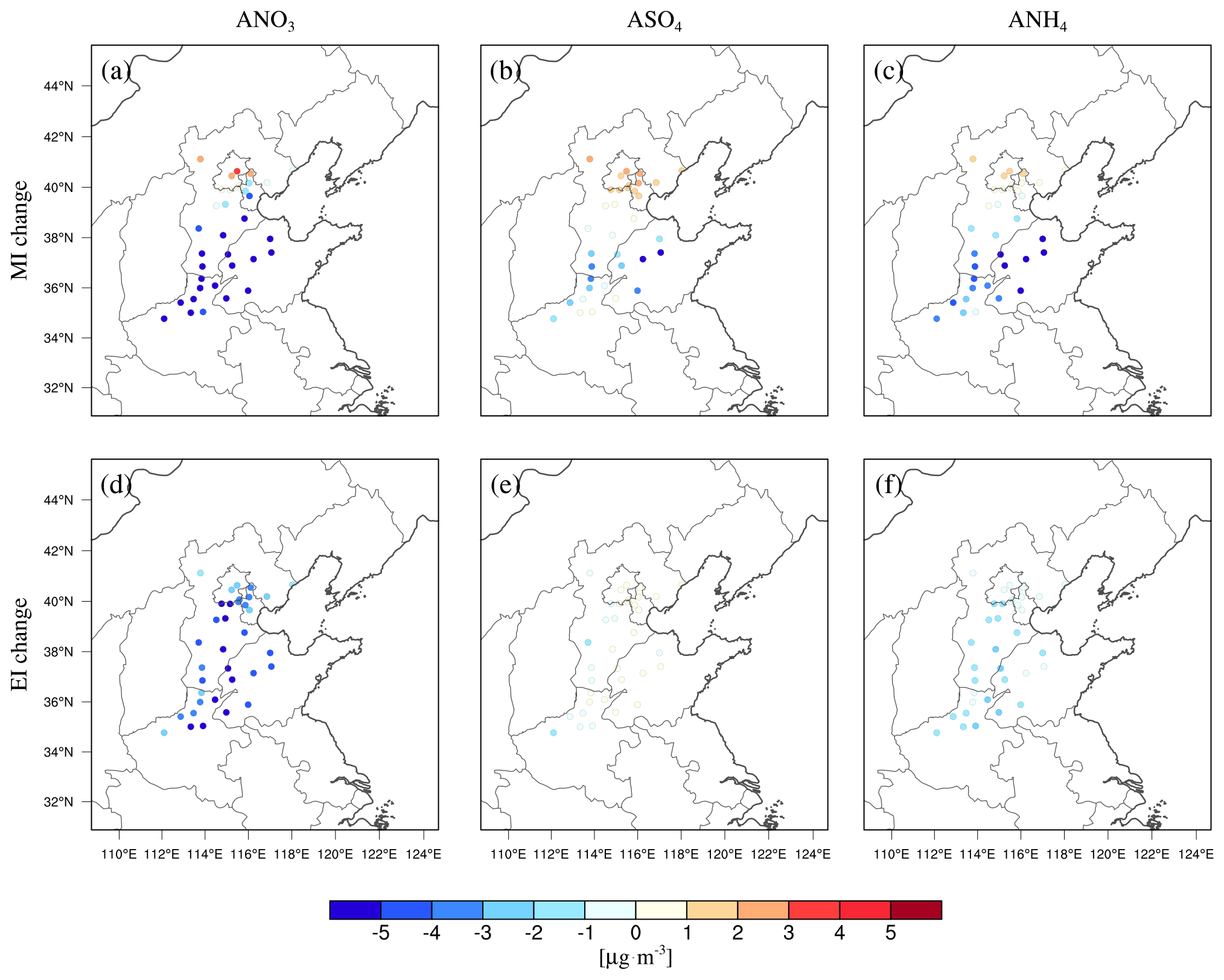
Figure 13 Meteorology-induced (MI) changes in the concentrations of (a) ANO₃, (b) ASO₄ and (c) ANH₄, as well as emission-induced (EI) changes in the concentrations of (d) ANO₃, (e) ASO₄ and (f) ANH₄.

4 Conclusions and discussions

The COVID-19 pandemic is an unprecedented event that significantly influenced social activity and the associated emissions of air pollutants. Our results provide a quantitative assessment of the influences of COVID-19 restrictions on multi-air-pollutant emissions in China. Otherwise, understanding the relationship between air quality and human activities may be biased. The inversion results provide important evidence that the COVID-19 lockdown policy was largely a traffic control measure with substantially reduced impacts on NO_x emissions but much smaller influences on the emissions of other species and other sectors. Traffic control has widely been considered to be the normal protocol in implementing regulations in many cities of China, but its effectiveness for air pollution control is still disputed (Han and Naeher, 2006; Zhang et al., 2007; Chen et al., 2021; Cai and Xie, 2011; Chowdhury et al., 2017; X. Li et al., 2017). Thus, the COVID-19 restrictions provided us with a real nationwide traffic control scenario to investigate the effectiveness of traffic control on the mitigation of air pollution in China. The results suggested that traffic control as a separate pollution control measure has limited effects on the coordinated control of high concentrations of O₃ and PM_2.5 under the current air pollution conditions in China. In this case, the PM_2.5 concentrations were slightly reduced, while there were substantial increases in O₃ concentrations. Severe haze was also not avoided during the COVID-19 restrictions due to unbalanced emission changes from other sectors and unfavorable meteorological conditions. China is now facing major challenges in both controlling PM_2.5 and controlling emerging O₃ pollution. The tragic COVID-19 pandemic has revealed the limitation of the road traffic control measures in the coordinated control of PM_2.5 and O₃. More comprehensive regulations for multiple precursors from different sectors are required in the future to address O₃ and PM_2.5 pollution in China.

Finally, there are certain limitations that we should be aware of in our inversion work. Firstly, the COVID-19 restrictions were initiated during the Spring Festival of China which would also influence the air pollutant emissions in China. However, the inversion method used in this study did not differentiate between the contributions of the Spring Festival from the COVID-19 restrictions. Similarly, the effects of natural emission changes were not differentiated in this study, which could lead to uncertainty in quantifying the effects of the COVID-19 restrictions on air pollutant emissions. Secondly, the overestimations of NO₂ measurements induced by chemiluminescence monitor interference were not directly corrected in our study due to the lack of synchronous observations of HNO₃, PAN and AN; thus the estimated NO_x emissions could be slightly overestimated according to the sensitivity run with corrected NO₂ measurements using CFs (Figs. S16–S18). Meanwhile, the sensitivity results suggest that the inversed NO_x emissions may even drop faster if the NO₂ measurements were corrected over the SE and SW regions (Fig. S19). Thirdly, the use of an outdated emission inventory as the a priori emissions would also be a potential limitation in our work, although the iteration inversion method was used. A sensitivity inversion run was thus conducted based on the a priori emissions for a more recent year of 2018 to test the influence of the a priori emission inventory. This new emission inventory is comprised of the anthropogenic emissions obtained from HTAPv3 (Crippa et al., 2023); the biogenic, soil and oceanic emissions obtained from the CAMS global emission inventory (https://ads.atmosphere.copernicus.eu/cdsapp#!/dataset/cams-global-emission-inventories?tab=overview, last access: 15 March 2023); and the biomass burning emissions obtained from the Global Fire Assimilation System (GFAS) (Kaiser et al., 2012). Detailed steps of the new inversion estimation were the same as those elucidated in Sect. 2. The results suggest that the inversion results based on the 2010 and 2018 inventory were broadly close to each other, while the inversion results based on the 2018 inventory were relatively higher than those based on the 2010 inventory, reflecting the uncertainty in our inversion results caused by the choice of a priori emission inventory (Figs. S20–S22). However, the sensitivity run consistently showed that the NO_x emissions decreased much more than other species (Figs. S23–S24). This suggests that the choice of a priori emission inventory may not obviously influence the main conclusion of our study but can lead to uncertainty in the magnitude of the inversion results, which potential readers should be aware of.