A new insight into the vertical differences in NO₂ heterogeneous reaction to produce HONO over inland and marginal seas

Ship-based multi-axis differential optical absorption spectroscopy (MAX-DOAS) measurements were conducted along the marginal seas of China from 19 April to 16 May 2018 to measure the vertical profiles of aerosol, nitrogen dioxide (NO₂), and nitrous acid (HONO). Along the cruise route, we found five hot spots with enhanced tropospheric NO₂ vertical column densities (VCDs) in the Yangtze River Delta, Taiwan Strait, Guangzhou–Hong Kong–Macau Greater Bay Area, port of Zhanjiang, and port of Qingdao. Enhanced HONO concentrations could usually be observed under high-level aerosol and NO₂ conditions, whereas the reverse was not always the case. To understand the impacts of relative humidity (RH), temperature, and aerosol on the heterogeneous reaction of NO₂ to form HONO in different scenarios, the Chinese Academy of Meteorological Sciences (CAMS) and Southern University of Science and Technology (SUST) MAX-DOAS stations were selected as the inland and coastal cases, respectively. The RH turning points in CAMS and SUST cases were both ∼ 65 % (60 %–70 %), whereas two turning peaks (∼ 60 % and ∼ 85 %) of RH were found in the sea cases. As temperature increased, the HONO $/$ NO₂ ratio decreased with peak values appearing at ∼ 12.5^∘C in CAMS, whereas the HONO $/$ NO₂ gradually increased and reached peak values at ∼ 31.5^∘C in SUST. In the sea cases, when the temperature exceeded 18.0^∘C, the HONO $/$ NO₂ ratio rose with increasing temperature and achieved its peak at ∼ 25.0^∘C. This indicated that high temperature can contribute to the secondary formation of HONO in the sea atmosphere. In the inland cases, the correlation analysis between HONO and aerosol in the near-surface layer showed that the ground surface is more crucial to the formation of HONO via the heterogeneous reaction of NO₂; however, in the coastal and sea cases, the aerosol surface contributed more. Furthermore, we discovered that the conversion rate of NO₂ to HONO through heterogeneous reactions in the sea cases is larger than that in the inland cases in higher atmospheric layers (> 600 m). Three typical events were selected to demonstrate three potential contributing factors of HONO production under marine conditions (i.e., transport, NO₂ heterogeneous reaction, and unknown HONO source). This study elucidates the sea–land and vertical differences in the forming mechanism of HONO via the NO₂ heterogeneous reaction and provides deep insights into tropospheric HONO distribution, transforming process, and environmental effects.

1 Introduction

Nitrous acid (HONO) is an important part of the atmospheric nitrogen cycle and plays a significant role in atmospheric oxidation capacity (Alicke et al., 2003; Kleffmann et al., 2005). Photolysis of HONO in near-ultraviolet bands (Reaction R1) is a substantial source of hydroxyl radicals (OH radicals), which are one of the most important oxidants in the tropospheric atmosphere. Earlier studies reported that the contribution of HONO photolysis to OH radicals can reach 40 %–60 %, while exceeding 80 % in the early morning (Michoud et al., 2012; Ryan et al., 2018; Xue et al., 2020). OH radicals can oxidize and destroy most atmospheric pollutants, such as CO, NO_x (NO + NO₂), SO₂, and volatile organic compounds (VOCs), thereby further promoting the formation of secondary pollutants (e.g., ozone (O₃), peroxyacetyl nitrate (PAN), and secondary aerosols) and leading to serious haze pollution events (Huang et al., 2014). Additionally, as a nitrosating agent, HONO can produce carcinogenic nitrite amines that pose a threat to human health (Zhang et al., 2015). Therefore, a full understanding of the source and formation mechanism of HONO is scientifically significant for the study of tropospheric oxidation and the control of secondary pollution.

Currently, the known sources of HONO mainly include direct emissions from vehicles, ships, biomass burning, and soil; the homogeneous reaction of NO and OH radicals (Reaction R2); the nighttime and daytime heterogeneous reaction of NO₂ (Reaction R3) on aerosols, vegetation, the ground, and other types of surfaces; and the photolysis of nitrate particles (Reaction R4) (Alicke et al., 2003; Stemmler et al., 2006; Indarto, 2012; Wang et al., 2015; Salgado and Rossi, 2002; Zhou et al., 2011). Sources of HONO exist that are poorly understood (Fu et al., 2019). The heterogeneous reaction of NO₂ as a source of HONO has received continuous attention in recent years. It was found that the heterogeneous reaction of NO₂ is one of the most important sources of HONO in a variety of scenes such as inland, coastal cities, and offshore seas. Liu et al. (2021) reported the contribution of the heterogeneous reaction of NO₂ on the aerosol surface to HONO is 19.2 % in summer, and this contribution on aerosol and ground surfaces to HONO can reach 54.6 % in winter in Beijing. Yang et al. (2021) and Zha et al. (2014) found that the generation rate of HONO through the heterogeneous reaction of NO₂ under sea-wind conditions could elevate 3–4 times more than that under land-wind conditions in the northern coastal city of Qingdao and the southern coastal city of Hong Kong, respectively. Cui et al. (2019) illustrated that the heterogeneous reaction of NO₂ on aerosol and sea surfaces is an important source of HONO in the East China Sea in summer. The process of HONO formed from the heterogeneous reaction of NO₂ is affected by various atmospheric parameters. The relative humidity (RH), temperature, solar radiation intensity (SRI), and aerosol concentration and its relative surface area are the particularly important parameters. Earlier works always used the linear regression relationship between HONO $/$ NO₂ and the above parameters to characterize the influence of these parameters on the formation of HONO through the heterogeneous reaction of NO₂. Although this kind of simple linear regression method may lead to artificial correlations and misleading conclusions, considering the vertical evolution of atmospheric parameters. Wen et al. (2019) found that the increased temperature could promote the heterogeneous reaction of NO₂ to form HONO in sea conditions. The generation rate of HONO could increase rapidly, when the temperature was greater than 20 ^∘C. Gil et al. (2019) found that the HONO formed from the heterogeneous reaction of NO₂ will increase along with the increase in RH when RH was less than 80 % in a case of a land park using deep learning forced by measurement results. Fu et al. (2019) reported that RH and SRI were the main parameters driving the heterogeneous reaction of NO₂ to form HONO in the Pearl River Delta, and it contributes 72 % of the total source of HONO. Cui et al. (2019) found that the potential of the heterogeneous reaction of NO₂ to form HONO will increase with the increase in particle concentration and the specific surface area of single particles in coastal cities.

$$\begin{array}{}\text{(R1)}& {\displaystyle }\mathrm{HONO}+hv\to \mathrm{NO}+\mathrm{•}\mathrm{OH}(\mathit{\lambda }<\mathrm{400}\mathrm{nm})\text{(R2)}& {\displaystyle }\mathrm{•}\mathrm{OH}+\mathrm{NO}+\mathrm{M}\to \mathrm{HONO}+\mathrm{M}\text{(R3)}& {\displaystyle }\mathrm{2}{\mathrm{NO}}_{\mathrm{2}}+{\mathrm{H}}_{\mathrm{2}}\mathrm{O}\to \mathrm{HONO}+{\mathrm{HNO}}_{\mathrm{3}}\text{(R4)}& {\displaystyle }\begin{array}{rl}& {\mathrm{HNO}}_{\mathrm{3}}/{\mathrm{NO}}_{\mathrm{3}}^{-}+hv\to \mathrm{HONO}/{\mathrm{NO}}_{\mathrm{2}}^{-}+\mathrm{O}\mathrm{•}\\ & (\mathit{\lambda }\sim \mathrm{300}\mathrm{nm})\end{array}\end{array}$$

However, earlier research generally focused on the near-surface layer of a single scene, and attention to the influence mechanism of the heterogeneous reaction of NO₂ to form HONO in the vertical direction and in different sea and land scenes is insufficient, which limits the comprehensive assessment to understand the sea–land differences and impact mechanism of HONO formed from the heterogeneous reaction of NO₂. NO₂ could be transported from inland and coastal cities to offshore seas (Tan et al., 2018). This part of NO₂ can promote the HONO formation through heterogeneous reactions on the high-level aerosol and sea surfaces in the sea atmosphere (Zhang et al., 2020). The formed HONO is likely to be carried to land cities at night by the sea breeze, which will affect the atmospheric oxidation and air quality and even endanger human health. Additionally, the vertical distributions and values of atmospheric meteorology and aerosol parameters are significantly different in land and sea scenes, which provide different conditions for the heterogeneous reaction of NO₂ to form HONO in different height layers. Furthermore, aerosols and NO₂ have complex evolution and transmission characteristics in the vertical direction. The vertical upward transport of aerosol and NO₂ can promote the HONO formation through heterogeneous reactions at high altitude, and the vertical downward transport of HONO will impact the atmospheric environment near the ground. The vertical observations in land and sea scenes are also helpful to distinguish the contribution of the heterogeneous reaction of NO₂ on the aerosol, ground, or sea surfaces (Zhang et al., 2020).

Currently, a variety of HONO measurement techniques have been developed, which in principle can be roughly divided into wet chemical, spectroscopy, and mass spectrometry methods (Cheng et al., 2013; Bernard et al., 2016; Gil et al., 2019; Guo et al., 2020; Jordan and Osthoff, 2020). However, these technical methods can only measure the HONO information near the surface layer. Taking tower and aircraft as platforms, these techniques were performed to measure HONO vertical profiles, and it was found that the peak values of HONO usually appeared under 200 m in urban and suburban areas (Kleffmann et al., 2003; Stemmler et al., 2006; Zhang et al., 2009; Wong et al., 2012; Meng et al., 2020; Zhang et al., 2020). These studies also revealed that the heterogeneous reaction of NO₂ on multiple surfaces (ground, aerosol, etc.) was an important source of HONO under the planetary boundary layer (PBL), especially during haze days. Furthermore, they also reported that the HONO $/$ NO₂ ratios usually decreased with the increase in height under 200 m in inland and coastal areas. However, the cost of the above techniques used to measure HONO vertical profiles was too high, and the real-time and continuous measurements cannot be realized. Multi-axis differential optical absorption spectroscopy (MAX-DOAS), as a ground-based ultra-hyperspectral remote sensing technology, has been widely used for the vertical observation of atmospheric pollutants in the past two decades. In the past 5 years, several researchers carried out campaigns based on MAX-DOAS to measure the vertical profile of HONO in inland and coastal areas, and they revealed their vertical characteristics, sources, and the contribution to atmospheric oxidation at different height layers (Garcia-Nieto et al., 2018; Ryan et al., 2018; Wang et al., 2020; Xing et al., 2021; Xu et al., 2021; He et al., 2023). Few studies were conducted on the sources of HONO at different height layers in sea conditions. In this study, MAX-DOAS is used for the first time to study the spatiotemporal distribution and the sources of HONO along the Chinese coastline, as well as to learn the differences in the HONO formed from the heterogeneous reaction of NO₂ in different height layers and land and sea scenes.

2 Methods and methodologies

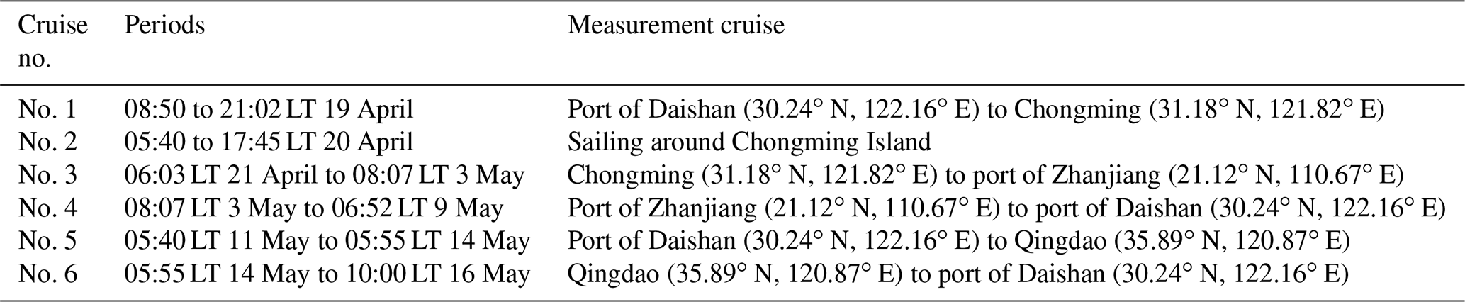
2.1 Measurement cruise

The ship-based atmospheric observation campaign along the marginal seas of China was conducted from 19 April to 16 May 2018. The latitude and longitude ranges of the entire campaign covered 21.12–35.89^∘ N and 110.67–122.16^∘ E. The detailed voyage records of the observation ship are shown in Table 1. An integrated and fully automated MAX-DOAS instrument was installed on board the stern deck of the ship (Fig. S1a in the Supplement). To ensure that the instrument was always kept in a horizontal position, a photoelectric gyro was used. The angle between the observation and heading direction of the ship was always maintained at 135^∘ during the whole campaign. The telescope unit of the instrument pointed towards the sea during cruise no. 3 and no. 6. The telescope unit pointed towards the land during cruise no. 1, no. 4, and no. 5. During cruise no. 2, the observation telescope always pointed to Chongming Island. The measurement ship only sailed during daytime from 19 April to 2 May and continuously sailed during the entire daytime and nighttime from 3 to 16 May 2018. The ship docked in the port of Daishan on 9–10 May, and no observations were conducted during these 2 d.

Table 1 Detailed information of the measurement cruises.

The aim of this campaign was to learn the vertical differences in the NO₂ heterogeneous reaction to produce HONO in marginal seas of China and compare the influence mechanism of that in inland cities. To fully understand the differences of the impacts of RH, temperature, and aerosol on the HONO secondary formation in land and sea conditions, the Chinese Academy of Meteorological Sciences (CAMS) and Southern University of Science and Technology (SUST) MAX-DOAS stations were selected as inland and coastal areas for analysis, respectively. CAMS is located in the urban area of Beijing (39.94^∘ N, 116.32^∘ E), and SUST is located in Shenzhen (22.60^∘ N, 114.00^∘ E) (Fig. S2). This study will provide scientific guidance for understanding regional oxidation capacity and controlling the secondary air pollution.

2.2 MAX-DOAS measurements

2.2.1 Instrument setup

The compact instrument consists of an ultraviolet spectrometer (AvaSpec-ULS2048L-USB2, 300–460 nm spectral range, 0.6 nm spectral resolution) at a 20^∘C fixed temperature with a deviation of < 0.01^∘C, a one-dimensional charge-coupled device (CCD) detector (Sony ILX511, 2048 individual pixels), and a telescope unit driven by a stepper motor to collect scattered sunlight from different elevation angles. The accuracy of elevation angle is < 0.1^∘, and the telescope field of view (open angle) is < 0.3^∘. A full scanning sequence consists of 11 elevation angles (1, 2, 3, 4, 5, 6, 8, 10, 15, 30, and 90^∘). The integration time of one individual spectrum was set to 30 s, and each scanning sequence took about 5.5 min. Besides, the controlling electronic devices and connecting fiber are mounted inside. The instrument is equipped with a high-precision global position system (GPS) to record the real-time coordinated positions of the cruise ship. The detailed description of the setup of MAX-DOAS in CAMS and SUST can be found in Liu et al. (2021).

2.2.2 Data processing and filtering

The MAX-DOAS measurements could be influenced by the exhaust from the measurement ship. Therefore, the data contaminated by the exhaust were filtered out. As shown in Fig. S1b, the direction and speed of the plume exhausted from the ship depend on the ship and the true wind speeds and directions. Individual measurements taken under unfavorable plume directions (plume directions between 45 and 135^∘ with respect to the heading of the ship) were discarded. To avoid the strong influence of the stratospheric absorption, the spectra measured with solar zenith angle (SZA) larger than 75^∘ were filtered out. Under these two filtering criteria, 4.9 % and 8.3 % of all data were rejected before DOAS analysis (Xing et al., 2017, 2019, 2020).

2.2.3 DOAS analysis

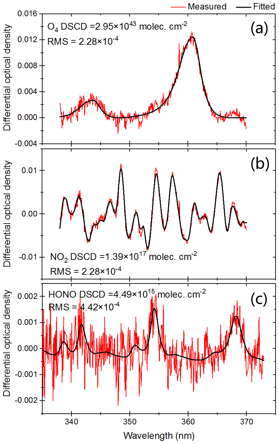
The MAX-DOAS measured spectra were analyzed using the software QDOAS which is developed by BIRA-IASB (http://uv-vis.aeronomie.be/software/QDOAS/, last access: 24 May 2023). The DOAS fit results are the differential slant column densities (DSCDs), i.e., the difference of the slant column density (SCD) between the off-zenith and the corresponding zenith reference spectra. Details of the DOAS fit settings are listed in Table 2. A typical DOAS retrieval example for the oxygen dimer (O₄), nitrogen dioxide (NO₂), and nitrous acid (HONO) is shown in Fig. 1. The stratospheric contribution was approximately eliminated by taking the zenith spectra of each scan as a reference in the DOAS analysis. Before profile retrieval, DOAS fit results of O₄, NO₂, and HONO with root mean square (RMS) of residuals larger than 3 × 10⁻³ were filtered. Furthermore, the SCD data under the color index (CI) being < 10 % of the thresholds obtained through fitting a fifth-order polynomial to CI data, which is a function of time, were filtered out to ensure a high signal-to-noise ratio (SNR) of the spectra. This filtering criteria remove 2.1 %, 3.9 %, and 5.3 % for O₄, NO₂, and HONO, respectively.

Table 2 Detailed retrieval settings of O₄, NO₂, and HONO.

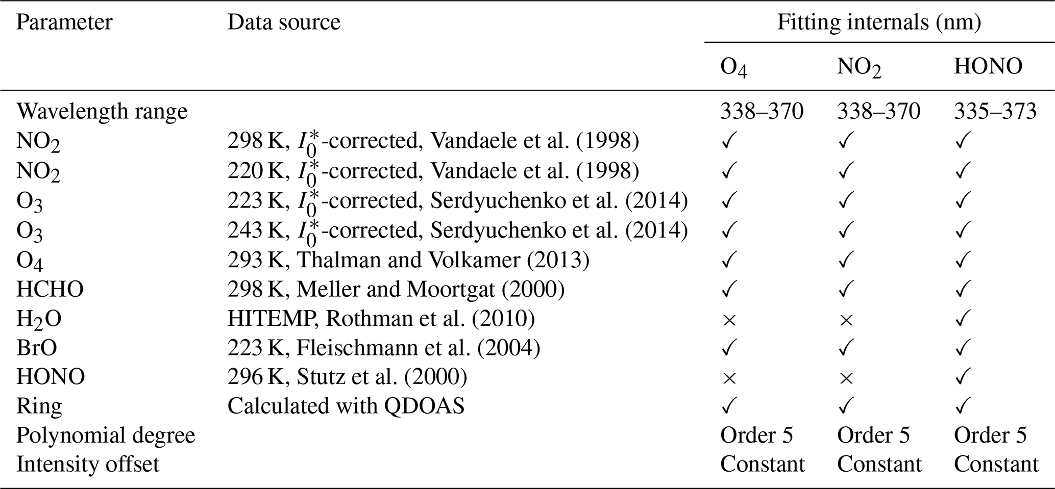
^∗ Solar I₀ correction; Aliwell et al. (2002).​​​​​​​

Figure 1 Plots depicting typical DOAS spectral fittings for (a) O₄, (b) NO₂, and (c) HONO.

2.3 Vertical profile retrieval

Aerosol and trace gas (i.e., NO₂ and HONO) vertical profiles are retrieved from MAX-DOAS measurements using the algorithm reported by Liu et al. (2021). The inversion algorithm is developed based on the optical estimation method (OEM) (Rodgers, 2000), which employs the radiative transfer model VLIDORT as the forward model. The detailed retrieval procedure is displayed in Sect. S1 and Fig. S3.

In this study, an exponentially decreasing a priori profile with a scale height of 1.0 km was used as the initial profile for both the aerosol and trace gas retrievals (Fig. S4). The surface concentrations of aerosol, NO₂, and HONO were set to 0.2 km⁻¹, 3.0 ppb, and 1.0 ppb, respectively. We assume a fixed set of aerosol optical properties with an asymmetry parameter of 0.69, a single scattering albedo of 0.90, and ground albedo of 0.05. Furthermore, the uncertainty of the aerosol and trace gas a priori profile was set to 100 %, and the correlation length was set to 0.5 km. The averaging kernels indicated that the sensitivity of the profile retrieval tended to decrease with increasing altitude and the retrieval especially sensitive to the layers within 0–1.5 km (Fig. S5). The sum of the diagonal elements in the averaging kernel matrix is the degree of freedom (DOF), which denotes the number of independent pieces of information contained in the measurements.

2.4 Error analysis

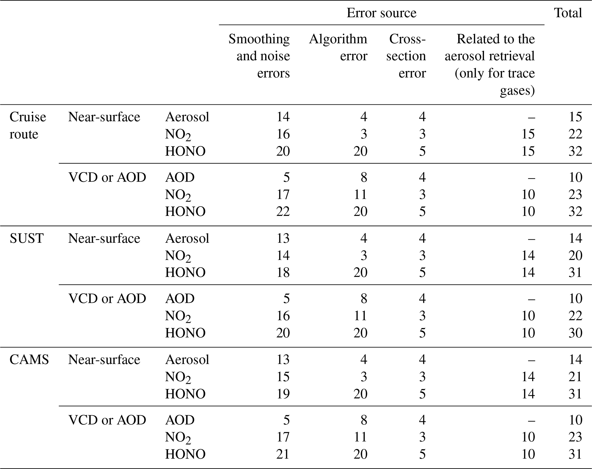
For profile retrieval, the error sources can be divided into four different types: smoothing error, measurement noise error, forward model error, and model parameter error (Frieß et al., 2006). However, in terms of this classification, some errors are difficult to calculate or estimate. For example, forward model error, which is caused by an imperfect representation of the physics of the system, is hard to quantify due to the difficulty of acquiring an improved forward model. Given calculation convenience and contributing ratios of different errors in total error budget, we mainly took into account error sources based on the following classification, which were smoothing and noise errors, algorithm error, cross-section error, and uncertainty related to the aerosol retrieval (only for trace gas). Here, we estimated the contribution of different error sources to the trace gas vertical column densities (VCDs) and aerosol optical depth (AOD), as well as near-surface (0–200 m) trace gas concentrations and aerosol extinction coefficients (AECs). The detailed demonstrations and estimation methods are displayed below, and the final results are summarized in Table 3.

• a.

  Smoothing errors arise from the limited vertical resolution of profile retrieval. Measurement noise errors denote the noise in the spectra (i.e., the fitting error of DOAS fits). They can be quantified by averaging the error of retrieved profiles, as the error of the retrieved state vector equals the sum of these two independent errors. We calculated the sum of smoothing and noise errors on near-surface concentrations and column densities, which were 14 % and 5 % for aerosols, 16 % and 17 % for NO₂, and 20 % and 22 % for HONO, respectively in the sea scene. The corresponding values were 13 % and 5 % for aerosols, 14 % and 16 % for NO₂, and 18 % and 20 % for HONO, respectively, at SUST and 13 % and 5 % for aerosols, 15 % and 17 % for NO₂, and 19 % and 21 % for HONO at CAMS.

• b.

  Algorithm error is the discrepancy between the measured and modeled DSCDs. This error contains the forward model error from an imperfect approximation of forward function (e.g., spatial inhomogeneities of absorbers and aerosols), forward model parameter error from the selection of parameters, and error not related to the forward function parameters, such as detector noise (Frieß et al., 2006). Algorithm error is a function of the viewing angle, and it is difficult to assign this error to each altitude of profile. Usually, the algorithm errors of the near-surface values and column densities are estimated by calculating the average relative differences between the measured and modeled DSCDs at the minimum and maximum elevation angles (except 90^∘) (Wagner et al., 2004). Considering its trivial role in the total error budget, we estimated these errors of the near-surface values and the column densities at 4 and 8 % for aerosols, 3 % and 11 % for NO₂, and 20 % and 20 % for HONO, according to Wang et al. (2017, 2020).

• c.

  Cross-section error is the error arising from an uncertainty in the cross section. According to Thalman and Volkamer (2013), Vandaele et al. (1998), and Stutz et al. (2000), we adopted 4 %, 3 %, and 5 % for O₄ (aerosols), NO₂, and HONO, respectively.

• d.

  The trace gas profile retrieval error represents the one which is sourced from aerosol extinction profile retrieval and propagated to retrieved trace gas profile. This error could be roughly estimated based on a linear propagation of the total error budgets of the aerosol retrievals. The errors of trace gases were roughly estimated at 15 % for VCDs and 10 % for near-surface concentrations for the two trace gases in the sea scene. The corresponding values were 14 % and 10 % for near-surface concentrations and VCDs, respectively, at SUST, and 14 % and 10 % at CAMS.

The total uncertainty was calculated by adding all the error terms in the Gaussian error propagation, and the final results were listed in the bottom row of Table 3. We found that the sum of smoothing and noise errors played a dominant role in the total uncertainty.

Table 3 Error budget estimation (in %) of the retrieved near-surface (0–200 m) trace gas concentrations and AECs, as well as trace gas VCDs and AOD.

2.5 Ancillary data

Meteorological data (including temperature, pressure, relative humidity, visibility, solar radiation intensity, wind speed, and wind direction) with a temporal resolution of 1 min were measured by the weather station installed on the ship. NO was measured using an NO analyzer (Thermo Scientific model 42i) with a 1 min resolution. The speed of the ship was calculated referring to the GPS data.

The temperature and relative humidity of two ground-based stations (i.e., CAMS and SUST) were collected from the Weather Underground website, the temporal resolution of which is around 3 h.

The backward trajectory was calculated using HYSPLIT (Hybrid Single-Particle Lagrangian Integrated Trajectory) developed by the National Oceanic and Atmospheric Administration Air Resource Laboratory (NOAA-ARL). The meteorological data with a 1^∘ × 1^∘ spatial resolution and 24 layers were collected from the Global Data Assimilation System (GDAS).

3 Results and discussion

3.1 Overview of the MAX-DOAS observations over marginal seas of China

The radiative transfer model SCIATRAN was used to convert SCDs of NO₂ and HONO to their tropospheric VCDs. The vertical profiles of aerosol, NO₂, and HONO retrieved from MAX-DOAS; the temperature and pressure vertical profiles simulated using a dynamical chemical model (WRF-Chem); and the geo-position data collected by GPS were introduced as inputs in SCIATRAN for the NO₂ and HONO air mass factor (AMF) calculation. Missing data are due to power and instrument system failure, interference of ship plume, unfavorable weather conditions (i.e., heavy rain), and night sailing. During the cruise of Chongming to Zhanjiang, NO₂ VCDs varied from 1.05 × 10¹⁴ to 4.02 × 10¹⁶ molec. cm⁻² with an averaged value of 3.90 × 10¹⁵ molec. cm⁻². From Zhanjiang to Qingdao, NO₂ VCDs varied from 1.08 × 10¹⁴ to 2.60 × 10¹⁶ molec. cm⁻² with an averaged value of 4.27 × 10¹⁵ molec. cm⁻². From Chongming to Zhanjiang, HONO VCDs varied from 1.00 × 10¹⁴ to 2.58 × 10¹⁵ molec. cm⁻² with a mean value of 2.39 × 10¹⁴ molec. cm⁻². From Zhanjiang to Qingdao, HONO VCDs varied from 1.01 × 10¹⁴ to 2.61 × 10¹⁵ molec. cm⁻² with a mean value of 2.74 × 10¹⁴ molec. cm⁻².

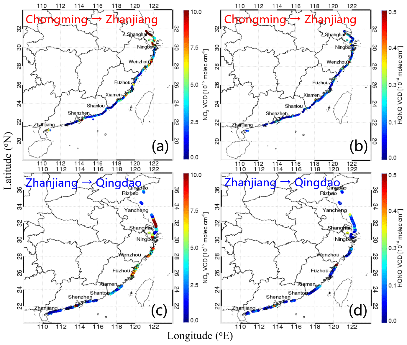
Figure 2 Maps showing the spatial distributions of NO₂ and HONO VCDs. Panels (a) and (b) show the NO₂ and HONO VCDs along the cruise route from Chongming to Zhanjiang. Panels (c) and (d) depict the NO₂ and HONO VCDs along the cruise route from Zhanjiang to Qingdao.

Figure 2 shows the spatial distribution of NO₂ and HONO VCDs over the marginal seas of China. Five enhanced tropospheric NO₂ VCD hot spots were observed during the whole campaign, i.e., the coastal areas of the Yangtze River Delta, Taiwan Strait, Guangzhou–Hong Kong–Macau Greater Bay Area, port of Zhanjiang, and port of Qingdao. In the coastal areas of Yangtze River Delta, the hot spots were mainly distributed in the Yangtze River estuary, Hangzhou Bay, port of Ningbo, port of Taizhou, and port of Wenzhou. These areas are mostly important shipping channels or shipping ports and are great NO₂ emission sources. The averaged NO₂ VCDs in the above five areas reached 1.07 × 10¹⁶, 1.30 × 10¹⁶, 7.27 × 10¹⁵, 5.34 × 10¹⁵, and 3.12 × 10¹⁵ molec. cm⁻², respectively (Fig. S6a). HONO exhibited similar spatial distribution characteristics as NO₂, and the averaged HONO VCDs in the above five hot-spot areas reached 1.01 × 10¹⁵, 7.91 × 10¹⁴, 6.02 × 10¹⁴, 5.36 × 10¹⁴, and 5.17 × 10¹⁴ molec. cm⁻², respectively (Fig. S6b). It indicates that NO₂ is an important precursor of HONO. Earlier studies reported that HONO can be generated from NO₂ through heterogeneous reactions on the surface of aerosol and the sea (Yang et al., 2021). However, there are obvious differences in the concentration distribution of HONO and NO₂ in the southeast coastal area of Jiangsu (from Qidong to Dongtai). In this area, NO₂ showed a higher concentration (1.66 × 10¹⁶ molec. cm⁻², which is 4 times higher than the mean NO₂ VCD), while HONO showed a lower concentration (2.06 × 10¹⁴ molec. cm⁻², which is ∼ 80 % of the mean HONO VCD). It may be the fresh ship emission plume on the route enhancing the NO₂ concentration and HONO had not been fully formed from the NO₂ heterogeneous reaction in time, since the observations from the ship-based MAX-DOAS are instantaneous.

The surface concentrations of NO₂ and HONO were extracted from their corresponding vertical profiles. As shown in Fig. 3, the total averaged near-surface NO₂ concentrations under sea-oriented and land-oriented measurements were 8.46 and 11.31 ppb, respectively. The total averaged near-surface HONO concentrations were 0.23 and 0.27 ppb under sea-oriented and land-oriented measurements. The total averaged near-surface HONO $/$ NO₂ ratios in sea-oriented and land-oriented measurements were 0.027 and 0.024, respectively. Earlier studies reported that vehicle and ship emissions were the main primary HONO sources on land and sea, respectively, and NO₂ heterogeneous reactions on the surfaces of the ground, sea, vegetation, and aerosol were the important secondary HONO sources (Liu et al., 2021). Additionally, Yang et al. (2021) found that the surface HONO concentrations in the sea cases were lower than that those in the land cases, especially in the morning and evening. Figure 4 shows the time series of AOD, the surface concentrations of NO₂ and HONO, and the surface HONO $/$ NO₂ during the whole campaign. We found that the time series of AOD and NO₂ were similar. The high AOD and NO₂ usually appeared in busy shipping channels and ports, and the obvious high-value areas were the coast of the Yangtze River Delta, the Taiwan Strait, port of Xiamen, port of Zhanjiang, and port of Qingdao (with mean AOD and NO₂ of 1.28 and 18.90 ppb, respectively). HONO always appeared under high AOD and NO₂ conditions; however, high AOD and NO₂ were not necessarily accompanied by a high HONO concentration. This was because the heterogeneous formation of HONO requires suitable meteorological conditions (i.e., RH and temperature) in addition to its precursor (NO₂) and the reaction surface (aerosol) (Liu et al., 2019). The high HONO $/$ NO₂ values were found on 2, 13, and 14 May with an average value of 0.45. Furthermore, we found the high values of HONO $/$ NO₂ always appeared from 11:00 to 14:00 LT (UTC+8)​​​​​​​ during the whole campaign.

Figure 3 Bar plots of the averaged aerosol extinction, NO₂ concentration, HONO concentration, and HONO $/$ NO₂ ratio during the campaign. The red and blue boxes denote sea-oriented and land-oriented measurements, respectively.

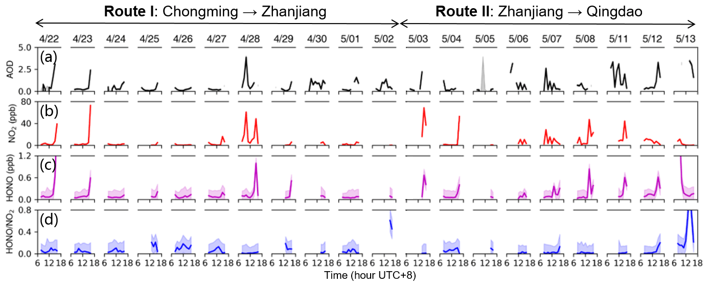
Figure 4 Histograms of the time series of (a) AOD, (b) surface NO₂ concentration, (c) surface HONO concentration, and (d) surface HONO $/$ NO₂ ratios.

3.2 Relationship between HONO $/$ NO₂ with RH, temperature, and aerosol for land and sea

Sun et al. (2020) reported that HONO concentrations could increase by up to 40 %–100 % over the shipping routes and international ports, and Huang et al. (2017) reported vehicle exhaust could contribute to ∼ 12 %–49 % of the atmospheric HONO budget. Since the direct emissions of the measurement ship were removed before data analysis, the primary source of HONO during the whole campaign was mainly from the direct emissions of cargo ships. By subtracting the average marine background of NO_x and HONO from the ship plume emission values, the impact of background values is reduced and the emission ratio of ΔHONO $/$ ΔNO_x can be obtained, and this emission ratio can be used for quantifying the primary HONO (Sun et al., 2020; Xu et al., 2015). In this study, we used an averaged 0.46 ± 0.31 % emission ratio of ΔHONO $/$ ΔNO_x referring to Sun et al. (2020) to understand the primary source of HONO on the sea surface during the campaign. The NO was measured using an in situ instrument, and sea surface NO₂ was extracted from the retrieved NO₂ vertical profiles (NO_x = NO + NO₂). Additionally, the calculation method of emission ratios of ΔHONO $/$ ΔNO_x in CAMS and SUST was taken from Xu et al. (2015), Liu et al. (2019), and Xing et al. (2021) (Sect. S2). The averaged emission ratios in CAMS and SUST were 0.82 ± 0.34 % and 0.79 ± 0.31 %, respectively. The direct emissions were deduced in the following study of the secondary formation of HONO. The ratios of HONO $/$ NO₂ in CAMS, SUST, and the ship-based campaign can be found in Fig. S7. Furthermore, the main secondary formation pathway of HONO is considered the heterogeneous reaction of NO₂ on the surface. The linear regression between HONO and NO₂ in the land and static sea scenarios is shown in Fig. 5. We found the fitting slopes in static sea scenes were ∼ 8–10 times larger than those in land scenes, especially for sea-oriented measurements under static weather conditions (slope ≈ 0.06). The correlation coefficients (R) in inland and static sea scenarios were all > 0.62, except in SUST (R = 0.58), which indicates the formation rate of secondary HONO from NO₂ heterogeneous reaction in static sea scenarios may be faster than that in land scenarios. The corresponding temperature and RH conditions of each spot are displayed in Fig. S8, which roughly reveals the impact of RH and temperature on the process of NO₂ forming HONO through heterogeneous reactions.

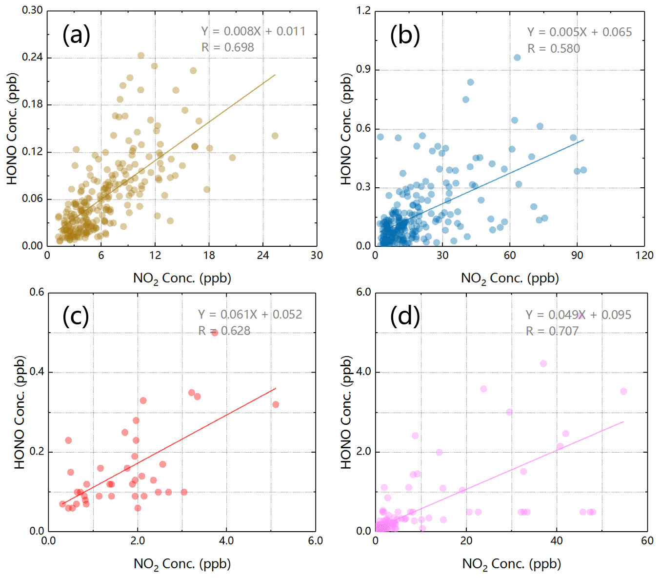
Figure 5 Linear regression plots between surface NO₂ and HONO concentrations in (a) CAMS, (b) SUST, and ship-based measurements of (c) sea-oriented and (d) land-oriented observations under static weather conditions.

3.2.1 RH dependence on HONO formation

The scatter plots of HONO $/$ NO₂ against RH in different land and sea conditions are illustrated in Fig. 6. The highest values can represent varying ranges of data in each interval and reveal concentration levels of data distribution. To eliminate the influence of other factors, the average of the six highest HONO $/$ NO₂ in each 10 % RH interval is calculated to reflect the distribution range of data in each interval (Liu et al., 2019). The dependence of the averaged top-six HONO $/$ NO₂ values on RH reveals an overall variation tendency of HONO $/$ NO₂ against RH. In the inland (CAMS) and coastal (SUST) cases, the RH turning points are both ∼ 65 % (60 %–70 %), where increasing trend switches to decreasing tendency. The HONO $/$ NO₂ increases along with RH when RH is less than 65 %, and the HONO $/$ NO₂ will decrease when RH is larger than 65 %, which implies that it contributes to the HONO formation from the heterogeneous reaction of NO₂ on wet surfaces with the gradual increase in RH until 65 %. The decrease in HONO $/$ NO₂ with RH larger than 65 % is presumably due to the efficient uptake of HONO on wet surfaces and the wet surfaces being less accessible or less reactive to NO₂ when RH is larger than 65 % (Liu et al., 2019). However, two turning peaks of RH were found in the sea cases. The first RH turning peak occurred in ∼ 60 %, which is similar to that in the inland and coastal cases, and another RH turning peak appeared in ∼ 85 % (80 %–90 %). This implies that high RH also could increase the HONO formation in sea cases. Additionally, the HONO $/$ NO₂ decreased sharply when RH was larger than 95 % because the reaction surface will asymptotically approach a water droplet state to limit the formation of HONO with RH larger than 95 %.

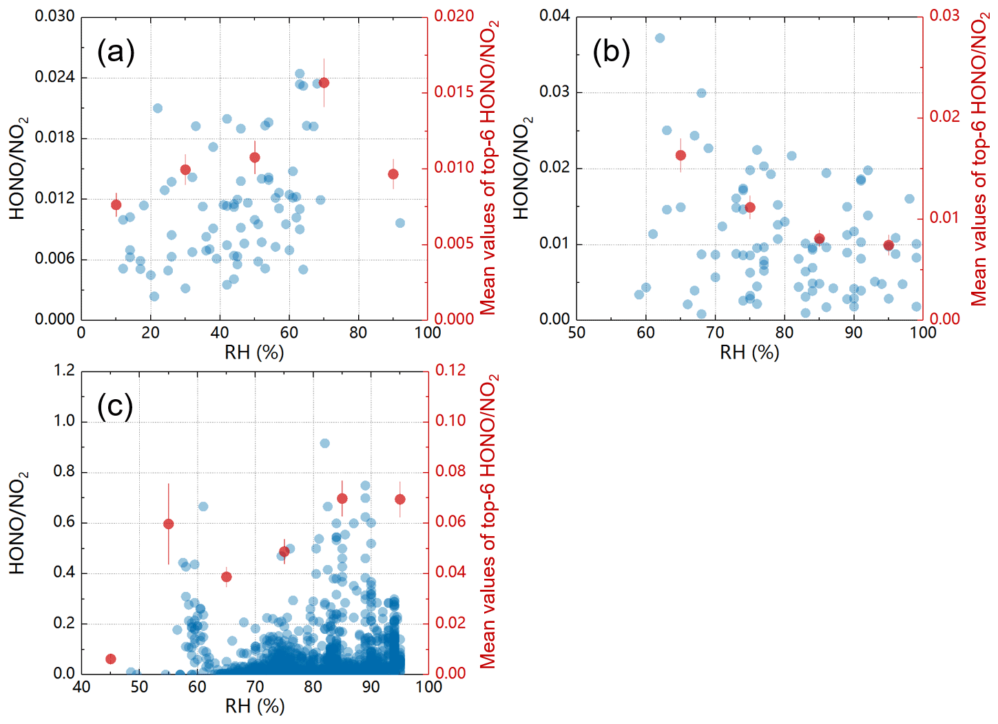
Figure 6 Scatter plots between RH and HONO $/$ NO₂ ratios for (a) CAMS, (b) SUST, and (c) the ship-based campaigns.

3.2.2 Temperature dependence on HONO formation

The scatter plots of HONO $/$ NO₂ against temperature in different land and sea conditions are shown in Fig. 7. Similar to the scatter plots of HONO $/$ NO₂ against RH, we also adopted the averaged top-six HONO $/$ NO₂ values in each 5^∘C interval to represent a general variation tendency of HONO $/$ NO₂ against temperature. In the inland condition (CAMS), the HONO $/$ NO₂ decreased along with the increase in temperature, and the highest values of HONO $/$ NO₂ appeared at ∼ 12.5^∘C. However, we found that HONO $/$ NO₂ increased along with the increase in temperature, and the highest values of HONO $/$ NO₂ appeared at ∼ 31.5^∘C in coastal conditions (SUST), which indicates that the HONO formation from NO₂ heterogeneous reaction will be accelerated under lower and higher temperature in the inland and coastal conditions, respectively. In the sea condition, the HONO $/$ NO₂ increased along with the increase in temperature with a high value under ∼ 25.0^∘C when the atmospheric temperature was higher than 18.0^∘C, and simultaneously, a ∼ 1.9 averaged HONO $/$ NO₂ high value was found under ∼ 15.0^∘C (14.0–17.0^∘C). Furthermore, we found that the appearance of HONO $/$ NO₂ high values under lower temperature (14.0–17.0^∘C) was usually accompanied by land breezes. Wen et al. (2019) also reported that relatively high temperature could contribute to the formation of HONO in the sea condition.

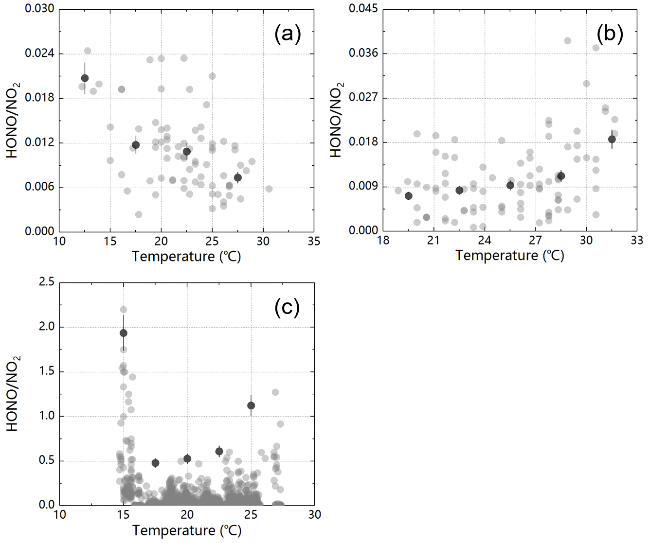
Figure 7 Scatter plots between temperature and HONO $/$ NO₂ ratios for (a) CAMS, (b) SUST, and (c) the ship-based campaigns.

3.2.3 Impact of aerosol on HONO formation

To further understand the HONO formation from the NO₂ heterogeneous reaction on the aerosol surface, several correlation analyses were conducted. As shown in Fig. 8, the linear regression plot between HONO and aerosol in land and sea conditions was performed. It was found that the correlation coefficient (R) between HONO and aerosol varied in the order of coastal (0.55) > sea (0.51) > inland (0.14). Additionally, the fitting slopes under coastal and sea conditions (0.07) are about 2.3 times larger than those under inland conditions (0.03), which implies that the ground surface may be more important than the aerosol surface during the process of HONO formed from NO₂ heterogeneous reactions in the ground surface layer inland. In the coastal and sea conditions, the aerosol and sea are both important in providing a heterogeneous reaction surface for NO₂ to form HONO (Cui et al., 2019; Wen et al., 2019; Yang et al., 2021). Additionally, we found the averaged values of HONO $/$ NO₂ were 0.011 ± 0.004, 0.014 ± 0.006, 0.008 ± 0.003, and 0.007 ± 0.003 when aerosol extinctions are 0–0.3, 0.3–0.6, 0.6–0.9, and > 0.9 km⁻¹ in the inland cases, respectively (Fig. 8b). As shown in Fig. 8, the high values of HONO $/$ NO₂ were mainly with aerosol extinction being less than 1.0 km⁻¹ with averaged values of 0.012 ± 0.006 and 0.090 ± 0.004 in the coastal and sea cases, respectively. It indicates that the aerosol surface plays a more important role in forming HONO through NO₂ heterogeneous reactions in the sea condition than that in the land condition.

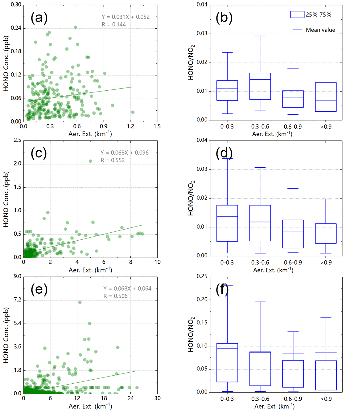
Figure 8 Panels (a), (c), and (e) show the linear regression plots between surface aerosol extinction and HONO concentrations for CAMS, SUST, and the ship-based campaigns, respectively. Panels (b), (d), and (f) depict the HONO $/$ NO₂ ratio distribution under different aerosol extinction coefficient conditions for CAMS, SUST, and the ship-based campaigns.

3.3 Vertical distributions of HONO $/$ NO₂ under different aerosol conditions for land and sea

To further investigate the height dependence of HONO $/$ NO₂ under land and sea conditions, two cases in the Pearl River Delta (PRD) were selected from the whole campaign. As shown in Fig. 9, “A” and “B” had a similar aerosol level (the extinction coefficients in the surface layer being 0.45–0.60 km⁻¹) and vertical distribution structure and were all observed from 10:00 to 11:00 LT. The instrument viewing the sea accompanied with sea wind in “A” is named the sea scene, and the instrument viewing the land accompanied with land wind in “B” is named the land scene. The NO₂ concentrations in the sea and land scenes have a similar vertical structure, and the NO₂ concentrations in the land scene are larger than those in the sea scene except on the surface layer. The HONO have the same vertical distribution structure in the above two scenes, and the HONO concentration in the land scene is always larger than that in the sea scene. In Fig. 9e, we found that HONO $/$ NO₂ under 0–400 m in the land scene is higher than that in the sea scene; however, the HONO $/$ NO₂ values are obviously lower in the land scene than those in the sea scene above 400 m. Furthermore, the growth rate of HONO $/$ NO₂ with the increase in height in the sea scene is significantly faster than that in the land scene above 400 m. This indicates the generation rates of HONO sourced from NO₂ heterogeneous reaction on the aerosol surface in the sea scene are larger than those in the land scene above 400 m. Under 400 m, the HONO generation rates in the land scene are larger than those in the sea scene.

Figure 9 Panel (a) shows the two measurement points (A: black, sea-oriented with sea wind; B: red, land-oriented with land wind) during the campaign. Panels (b)–(e) show the vertical profiles of aerosol, NO₂, HONO, and HONO $/$ NO₂ ratios in the above two measurement points, respectively.

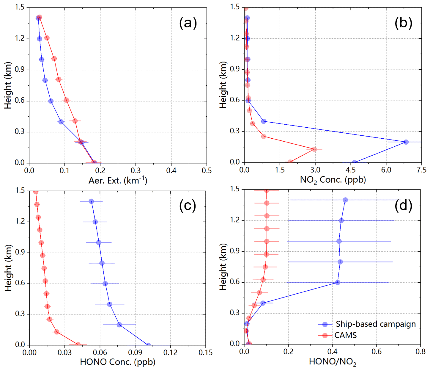
Figure 10 Plots showing the vertical distributions of (a) aerosol extinction, (b) NO₂ concentration, (c) HONO concentration, and (d) HONO $/$ NO₂ ratio. The blue and red lines represent a ship-based campaign case and a CAMS case, respectively.

Additionally, we selected inland cases (CAMS) to learn the difference in height dependence of HONO $/$ NO₂ compared with sea scenes with different aerosol loads. As shown in Fig. 10, the sea and inland scenes had similar aerosol levels (low aerosol level: < 0.2 km⁻¹) and vertical structure. Furthermore, the NO₂ and HONO in the sea and inland scenes have a similar vertical structure, although their concentrations in the sea scene are all larger than those in the inland scene. In Fig. 10d, we found that the HONO $/$ NO₂ in the sea scene was obviously larger than that in the inland scene above 400 m. The HONO $/$ NO₂ in the sea scene was about 4.5 times larger than that in the inland scene especially above 600 m. As shown in Fig. 11, the aerosols in the sea and inland scenes exhibited similar extinction levels (relatively high level: ∼ 0.8 km⁻¹) and vertical structure. The NO₂ concentration in the sea scene was higher than that in the inland scene but with a similar vertical structure. The HONO concentration in the sea scene was lower than that in the inland scene under 400 m, while the concentration in the sea scene was larger than that in the inland scene above 400 m. In Fig. 11d, we found the HONO $/$ NO₂ in the inland scene was larger than that in the sea scene under 600 m, while the HONO $/$ NO₂ in the sea scene was about 2 times larger than that in the inland scene above 600 m. All the above cases indicated that the HONO generation rate from NO₂ heterogeneous reaction in the sea scene was larger than that in the inland scene in higher atmospheric layers above 400–600 m. The high-altitude (> 400–600 m) atmospheric parameters in the sea scene were more conductive to promote the HONO formation through the heterogeneous reaction of NO₂. As shown in Fig. S9, the ratio of HONO $/$ NO₂ also generally increased with the increase in height above 0.2 km during the whole ship-based campaign. The greatest sensitivity under 1.5 km and the high DOF for aerosol, NO₂, and HONO gave confidence in the retrieval results (Fig. S10).

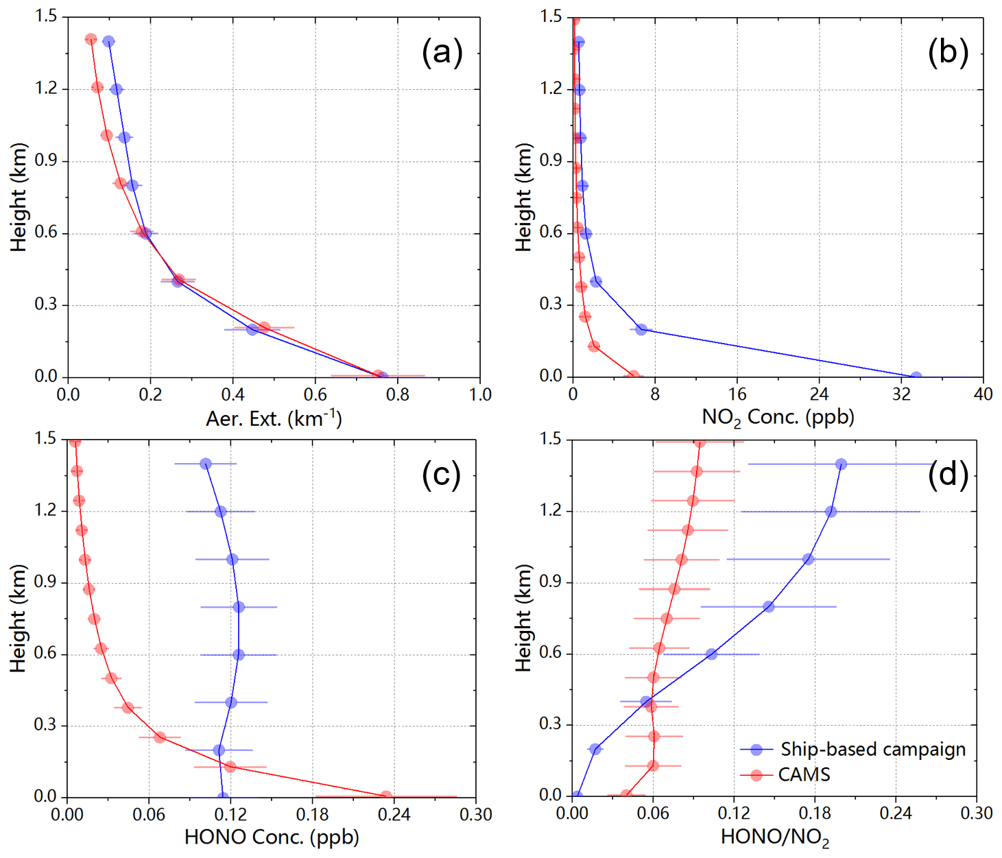
Figure 11 Plots showing the vertical distributions of (a) aerosol extinction, (b) NO₂ concentration, (c) HONO concentration, and (d) HONO $/$ NO₂ ratio. The blue and red lines represent a ship-based campaign case and a CAMS case, respectively.

3.4 Case study

The important factors and precursors to drive the formation of HONO through heterogeneous reactions had complex evolution and transport characteristics. To further clarify the role of these parameters in the heterogeneous process of NO₂ to form HONO, three typical processes were selected to reveal the favorable conditions for HONO formation in the sea scene.

3.4.1 20 April: a typical transport event

As shown in Fig. 12, the aerosol mainly distributed in 0–200 m with a mean extinction coefficient larger than 0.74 km⁻¹. NO₂ was mainly distributed near the ground surface with a mean concentration of 28.54 ppb before 13:20 LT. The NO₂ during this period may come from local ship emissions, as this area is a main shipping channel. From 14:25 to 17:10 LT, a high-concentration NO₂ air mass (average 13.29 ppb) was found at ∼ 2.0 km. To understand the source of this high-altitude NO₂ air mass, we further investigated the possible influence of transport by using the backward trajectories. We calculated 24 h backward trajectories of air masses at 500, 1000, and 2000 m using HYSPLIT (Fig. S11). In Fig. S11, we found that the dominant wind direction during this period was southeast at all heights, i.e., 500, 1000, and 2000 m. The transport of air masses carried NO₂ emitted by ships in the ports of Ningbo and Zhoushan to the main cargo ports of China and Shanghai. Furthermore, the concentration of NO₂ was low (averaged 2.32 ppb) near the ground surface from 14:25 to 17:10 LT. As shown in Fig. 12e and g, a low-pressure (< 1020 hPa), north-dominant wind direction with a wind speed > 12 m s⁻¹ appeared at the ground surface during this period, which implies that the clean air from the north reduced the local surface NO₂. The HONO was mainly distributed near the surface with a mean concentration of 0.07 ppb, and the two peaks were found in the early morning (averaged 0.15 ppb) and at 12:15 LT (averaged 0.11 ppb), respectively (Fig. S12). The relatively high concentration of HONO appearing in the early morning was possibly attributed to the accumulation with the stabilization of the boundary layer and attenuation of solar radiation after sunset the day before (Xing et al., 2021). The HONO peak appearing at 12:15 LT may be sourced from the heterogeneous reaction of NO₂ on the aerosol surface under a ∼ 80 % RH, 18.5^∘C temperature, and 1 × 10³ W m⁻² SRI conditions.

Figure 12 Case of 20 April 2018. Gradient images showing the time series of (a) aerosol extinction, (b) NO₂, and (c) HONO vertical profiles. Panel (d) shows the time series of surface RH. Panel (e) depicts the time series of surface temperature and pressure. Panel (f) shows the time series of surface SRI. Panel (g) depicts the time series of surface wind speed and wind direction.

3.4.2 28 April: a typical event of HONO produced from NO₂ heterogeneous reaction

From a typical port observation case, the measurement ship was moored at the port of Xiamen on 28 April. As shown in Fig. 13, we found two peaks for aerosol and NO₂ from 09:00–11:00 and 14:00–16:00 LT, respectively (averaged aerosol extinction coefficient > 0.8 km⁻¹, averaged NO₂ concentration > 12.0 ppb). NO₂ was mainly distributed near the sea surface layer at 0–200 m, and a high-concentration NO₂ air mass was found from 1.0–2.0 km from 13:00–14:00 LT due to the short-distance transport of NO₂ emitted from ships in the port of Xiamen (Fig. S13). However, aerosol appeared in the range of 0.0–2.0 km from 09:00–11:00 and 14:00–16:00 LT. In Fig. 13g, we found that the wind speeds in the above two peak periods were obviously higher than those in other periods. From 09:00–11:00 LT, the wind speed was ∼ 5.0 m s⁻¹ with a northwest-dominant direction (urban), and the wind speed was ∼ 6.0 m s⁻¹ with a southeast-dominant direction (port gateway) from 14:00–16:00 LT, which indicates that the short-distance high-altitude transport caused the appearance of high-extinction aerosol mass during the above two periods.

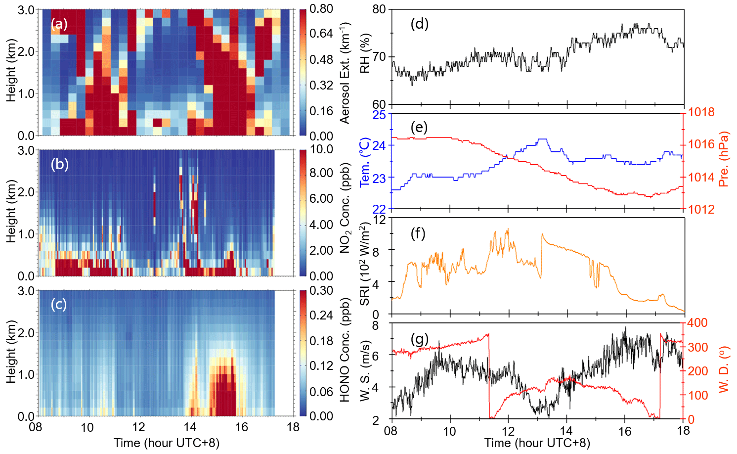
Figure 13 Case of 28 April 2018. Gradient images showing the time series of (a) aerosol extinction, (b) NO₂, and (c) HONO vertical profiles. Panel (d) shows the time series of surface RH. Panel (e) depicts the time series of surface temperature and pressure. Panel (f) shows the time series of surface SRI. Panel (g) depicts the time series of surface wind speed and wind direction.

Furthermore, we found the high-concentration HONO only appeared at 14:00–16:00 LT with a 0.57 ppb averaged concentration under 0.9 km, while it was only about 0.14 ppb during the 09:00–11:00 LT period. The slight increase in RH and temperature (Tem) at 14:00–16:00 LT (RH: ∼ 75.0 %; Tem: 23.7^∘C) may contribute more to HONO formation through heterogeneous reactions of NO₂ on the aerosol surface than that at 09:00–11:00 LT (Fig. 13d–e, Sect. 3.2). Contrarily, the SRI (∼ 600 W m⁻²) at 09:00–11:00 LT was obviously larger than that (∼ 250 W m⁻²) at 14:00–16:00 LT (Fig. 13f). The higher SRI accelerated the photolysis of HONO during the 09:00–11:00 LT period (Kraus and Hofzumahaus, 1998). Therefore, the lower formation rate and higher photolysis rate lead to a significantly lower HONO concentration at 09:00–11:00 LT than that at 14:00–16:00 LT.

3.4.3 3 May: a typical event with unknown HONO source

The measurement ship conducted observations in the sea area near Zhanjiang on 3 May, 2018. As shown in Fig. 14, we found that there was an obvious sinking process for aerosol from ∼ 1.0 km from 09:00–16:00 LT that eventually accumulated near the sea surface with a high extinction coefficient > 0.92 km⁻¹. The NO₂ was mainly concentrated near the sea surface layer (0–400 m) with an averaged concentration of 8.93 ppb from 08:00 to 09:00 LT. Thereafter, with the rise in the PBL height after sunrise, NO₂ was gradually mixed and spread throughout the PBL from 09:00–13:00 LT. During this period, it was accompanied by the increase in the NO₂ concentration (averaged 11.2 ppb) under the PBL (Fig. S14). It is due to the contribution of ship emissions near the sea surface. Contrarily, the regional transport of NO₂ from land also increased the NO₂ concentration in this area of the sea, with wind speed increasing from 2.5 to 7.8 m s⁻¹ with a north wind direction from 10:00 to 16:00 LT (Fig. 14g).

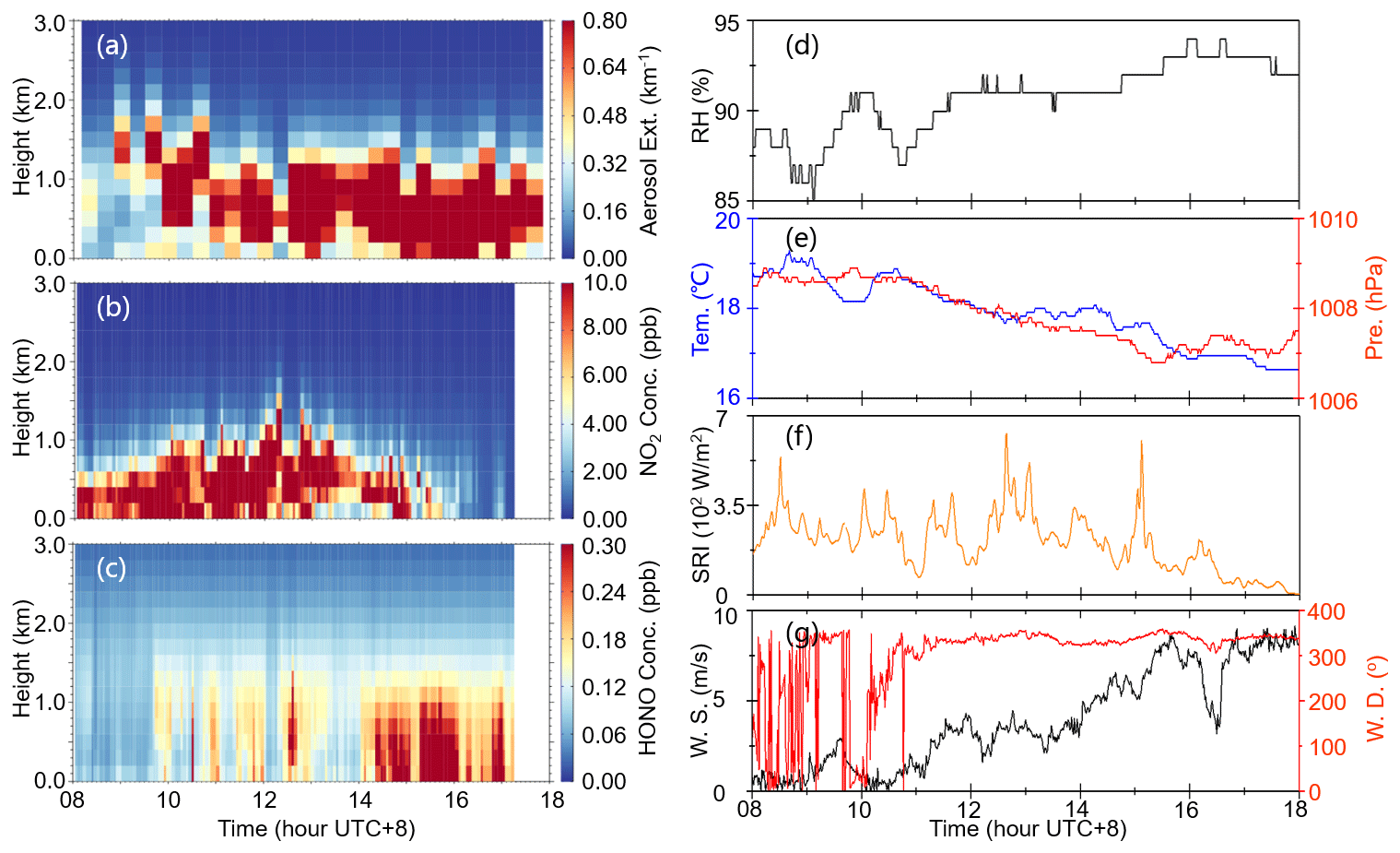
Figure 14 Case of 3 May 2018. Gradient images showing the time series of (a) aerosol extinction, (b) NO₂, and (c) HONO vertical profiles. Panel (d) shows the time series of surface RH. Panel (e) depicts the time series of surface temperature and pressure. Panel (f) shows the time series of surface SRI. Panel (g) depicts the time series of surface wind speed and wind direction.

Several HONO peaks (> 0.2 ppb) at 0.5–1.0 km were found from 09:45 to 13:00 LT, and the aerosol and NO₂ high values were also observed at this height layer, simultaneously, which implies that the heterogeneous reaction of NO₂ on the aerosol surface is more important than that on the sea surface for HONO source under sea atmosphere. Additionally, HONO concentration obviously elevated after 14:00 LT, especially from 14:00–16:00 LT (> 0.4 ppb). It may be sourced from the heterogeneous reaction of NO₂ on the aerosol surface, with RH being ∼ 92.5 % (Fig. 14d). The photolysis of HONO also decreased with SRI < 150 W m⁻² (Fig. 14f) during this period. Furthermore, a HONO peak (> 0.32 ppb) was observed from 16:40–17:10 LT. However, the NO₂ concentration always remained low (< 1.5 ppb) after 16:00 LT, and the temperature was lower than 17^∘C (Fig. 14e), which indicates the heterogeneous reaction of NO₂ not being the source of the observed HONO peak. The wind was north-dominant with an average speed at 7.8 m s⁻¹ after 15:00 LT, which implies that the regional transport may not be the source of the observed high-concentration of HONO. Furthermore, the SRI was lower than 87.5 W m⁻², and it shows the photolysis of nitrate aerosol also not being the source of the elevated HONO. The unknown HONO sources in this area of the sea need to be further explored.

4 Summary and conclusions

Currently, many uncertainties in the study of the HONO forming mechanism through the heterogeneous reaction of NO₂ exist. Earlier studies mostly focused on the near-surface layer, and the assessment of the contribution of the NO₂ heterogeneous reaction to HONO formation in the vertical direction of the boundary layer is insufficient. Therefore, we aim to learn the sea–land and vertical differences of the HONO forming mechanism from the NO₂ heterogeneous reaction and provide deep insights into the distribution characteristics, transforming process, and environmental effects of tropospheric HONO. Ship-based MAX-DOAS observations along the marginal seas of China were performed from 19 April to 16 May 2018. Simultaneously, two ground-based MAX-DOAS observations were conducted in the inland station CAMS and the coastal station SUST to measure the aerosol, NO₂, and HONO vertical profiles.

Along the cruise route, we found five hot spots with enhanced tropospheric NO₂ VCDs in the Yangtze River Delta, Taiwan Strait, Guangzhou–Hong Kong–Macau Greater Bay Area, port of Zhanjiang, and port of Qingdao. Under high-level NO₂ conditions in the above five hot spots, we also observed enhanced HONO levels. Contrastingly, the low-concentration HONO accompanied high-level NO₂ in the southeast coastline of Jiangsu province. When peak AOD and NO₂ conditions were observed, enhanced HONO was observed, although the reverse was not always the case.

To understand the impacts of RH, temperature, and aerosol on the heterogeneous reaction of NO₂ to produce HONO, the emission ratios of ΔHONO $/$ ΔNO_x were calculated to quantify the contribution of the primary HONO source to the total production of HONO. We found that the RH turning points in CAMS and SUST cases were both ∼ 65 % (60 %–70 %), whereas two turning peaks (∼ 60 % and ∼ 85 %) of RH were found in the sea cases. This implied that high RH could contribute to the secondary formation of HONO in the sea atmosphere. With an increase in temperature, the HONO $/$ NO₂ decreased with peak values appearing at ∼ 12.5^∘C in CAMS, whereas the HONO $/$ NO₂ gradually increased and reached peak values at ∼ 31.5^∘C in SUST. In the sea cases, when the temperature exceeded 18.0^∘C, the HONO $/$ NO₂ increased with the increasing temperature and achieved a peak at ∼ 25.0^∘C. This indicated that high temperature could promote the secondary formation of HONO in the sea and coastal atmosphere. Additionally, the correlation analysis under different sea–land conditions indicated that the ground surface is more crucial to the formation of HONO from the NO₂ heterogeneous reaction in the inland cases, whereas the aerosol surface contributed more in the coastal and sea cases.

Furthermore, we found that the HONO $/$ NO₂ in the sea cases was about 4.5 times larger than that in the inland cases above 600 m when the AEC was ∼ 0.2 km⁻¹, and the HONO $/$ NO₂ ratio in the sea cases was about 2 times larger than that in the inland cases above 600 m when the AEC was ∼ 0.8 km⁻¹, which implied that the generation rate of HONO from NO₂ heterogeneous reaction in the sea cases is larger than that in the inland cases in higher atmospheric layers (> 600 m). To have a deep understanding of three potential contributing factors of HONO production under marine conditions, we selected three typical events, which represented the impacts of transport, NO₂ heterogeneous reaction, and unknown HONO source.