the Creative Commons Attribution 4.0 License.
the Creative Commons Attribution 4.0 License.
 | 17 May 2023
Snowpack nitrate photolysis drives the summertime atmospheric nitrous acid (HONO) budget in coastal Antarctica
Jan Kaiser
Jörg Kleffmann
Anna E. Jones
Freya A. Squires
Measurements of atmospheric nitrous acid (HONO) amount fraction and flux density above snow were carried out using a long-path absorption photometer at Halley station in coastal Antarctica between 22 January and 3 February 2022. The mean ±1σ HONO amount fraction was (2.1 ± 1.5) pmol mol−1 and showed a diurnal cycle (range of 1.0–3.2 pmol mol−1) with a maximum at solar noon. These HONO amount fractions are generally lower than have been observed at other Antarctic locations. The flux density of HONO from the snow, measured between 31 January and 1 February 2022, was between 0.5 and 3.4×10¹² and showed a decrease during the night. The measured flux density is close to the calculated HONO production rate from photolysis of nitrate present in the snow. A simple box model of HONO sources and sinks showed that the flux of HONO from the snow makes a >10 times larger contribution to the HONO budget than its formation through the reaction of OH and NO. Ratios of these HONO amount fractions to NOx measurements made in summer 2005 are low (0.15–0.35), which we take as an indication of our measurements being comparatively free from interferences. Further calculations suggest that HONO photolysis could produce up to 12 of OH, approximately half that produced by ozone photolysis, which highlights the importance of HONO snow emissions as an OH source in the atmospheric boundary layer above Antarctic snowpacks.
- Article
(4590 KB) - Full-text XML
- BibTeX
- EndNote


Photolysis of nitrous acid (HONO) is a crucial polar boundary layer source of the hydroxyl radical (OH), a daytime oxidant that is important for the removal of many pollutants, including the greenhouse gas methane (CH4) (Kleffmann, 2007).
On a global scale, OH radical formation is usually controlled by ozone (O3) photolysis followed by reaction with water vapour:
The OH production by O3 photolysis is expected to be limited in the polar regions because in a cold atmosphere the water vapour concentration is low (Davis et al., 2008). It has been established that sunlit polar snowpacks are an important source of OH precursors for the lower atmosphere including NOx (Honrath et al., 1999; Jones et al., 2000) and HONO (Zhou et al., 2001), and formaldehyde (CH2O) and hydrogen peroxide (H2O2) (Hutterli et al., 2002, 2004; Frey et al., 2005). Unexpectedly high HONO amount fractions have been measured above snow surfaces in polar regions (Zhou et al., 2001; Honrath et al., 2002; Beine et al., 2001, 2002; Dibb et al., 2002, 2004; Kerbrat et al., 2012; Legrand et al., 2014) and also at mid-latitudes (Kleffmann et al., 2002; Kleffmann and Wiesen, 2008; Michoud et al., 2015; Chen et al., 2019).
In the boundary layer, HONO is formed through the homogeneous reaction of OH and NO:
At Arctic and Antarctic Plateau locations, this has been found to have a lower contribution to the HONO budget than emission from the snow (Villena et al., 2011; Legrand et al., 2014). However, the importance of different HONO sources is less clear in coastal Antarctica (Beine et al., 2006). The dominant HONO loss process is photolysis (Reaction R1), but it is also lost through reaction with OH:
The exact mechanism for HONO release from snow is not understood, and models of HONO sources and sinks often cannot rationalise the measured HONO amount fractions (Villena et al., 2011; Legrand et al., 2014). Nitrate photolysis in snow produces nitrite ():
which can be protonated to form HONO (Honrath et al., 2000; Zhou et al., 2001):
Correlations have been observed between snow nitrate concentrations and HONO formation (Dibb et al., 2002; Legrand et al., 2014). Several studies also report reduced HONO production from alkaline snow, which supports this mechanism (Beine et al., 2005, 2006; Amoroso et al., 2006). However, the dominant product from nitrate photolysis is nitrogen dioxide (NO2):
which can undergo hydrolysis to produce HONO via disproportionation (Finlayson-Pitts et al., 2003):
or reactions on organic surfaces in the snow (Ammann et al., 2005):
The uptake of NO2 on such organics is greater in the presence of sunlight (George et al., 2005):
The reaction of NO2 on photosensitised organics (Reaction R11) has been found to occur much faster than the disproportionation reaction (Reaction R9) (Stemmler et al., 2006). HONO formation from humic acid-doped ice films under a flow of NO2 was found to scale with both the NO2 and humic acid concentration (Beine et al., 2008; Bartels-Rausch et al., 2010). During their measurement campaign in Alaska, Villena et al. (2011) found a correlation between their calculated HONO snow-source strength and [NO2]×J(NO2), but not , suggesting that conversion of NO2 on photosensitised organic surfaces in the snow is the likely source of HONO (Reaction R11).
HONO amount fractions have been measured at both Arctic and Antarctic locations, and above mid-latitude snow covered areas. In Antarctica, HONO has been detected at inland and coastal locations, summarised in Fig. 1. Previous results from Halley Research Station, a coastal, ice-shelf location, gave average HONO amount fractions of 7 pmol mol−1 during the CHABLIS campaign in January–February 2005 (Bloss et al., 2010), but this was thought to be an overestimate due to chemical interferences in the wet-chemical HONO instrument used (Jones et al., 2011). On the Antarctic Plateau, HONO amount fractions are higher. At the South Pole, up to 18 pmol mol−1 HONO was measured by laser-induced fluorescence (LIF) (Liao et al., 2006), and at Dome Concordia (Dome C), more recent measurements using a long-path absorption photometer (LOPAP) yielded HONO amount fractions of 28 pmol mol−1 in austral summer 2010–2011 (Kerbrat et al., 2012) and 35 pmol mol−1 in 2011–2012 (Legrand et al., 2014). A strong diurnal cycle of HONO was observed in both measurement periods, with enhancements in the morning and evening suggesting a photochemical source. In contrast, at Dumont D'Urville (DDU), a coastal site without snow cover, HONO amount fractions were much lower, with a mean of 3 pmol mol−1 and no diurnal variation. However, the arrival of inland Antarctic air masses at DDU coincided with higher HONO amount fractions, supporting the existence of a HONO source in the continental snowpack (Kerbrat et al., 2012).

Figure 1A map showing the mean atmospheric HONO amount fractions (in pmol mol−1) measured previously in the Antarctic lower troposphere during summer (Dibb et al., 2004; Beine et al., 2006; Liao et al., 2006; Bloss et al., 2010; Kerbrat et al., 2012; Legrand et al., 2014).
There have been significant issues with the overestimation of atmospheric HONO amount fractions by various measurement techniques due to interferences. Measurements made at the South Pole with mist chamber sampling followed by ion chromatography analysis (MC/IC) gave 6 times higher values than those made by LIF (Dibb et al., 2004; Liao et al., 2006). At Halley, the wet-chemical method (scrubbing HONO into water, azo dye derivatisation, followed by optical detection) did not allow for interference removal, and hence, the HONO amount fractions were overestimated (Jones et al., 2011). In contrast, the two-channel concept of the long-path absorption photometer (LOPAP) used at Dome C and DDU is expected to correct for most interferences. In addition, the external sampling unit of this instrument minimises sampling artefacts, for example, those in sampling lines typically used for other HONO instruments. However, the high HONO amount fractions observed at Dome C were partially explained with potential interference of peroxynitric acid (HNO4). The interference of HNO4 in the LOPAP instrument has not been systematically studied, and the documented HNO4 interference of around 15 % may become an issue at lower temperatures due to its longer lifetime with respect to thermal decomposition (Legrand et al., 2014).
Further investigation is clearly needed to better understand HONO sources and sinks in the polar boundary layer, and the implications for the HOx budget. This paper presents measurements of HONO amount fractions and flux densities made at Halley during austral summer 2021–2022. A LOPAP instrument was used for this study to minimise interferences and sampling artefacts. The results are rationalised using knowledge of possible HONO sources, and the potential of HONO as an OH source to the boundary layer at Halley will be discussed.
2.1 Site
Our measurement campaign took place between 22 January and 3 February 2022 at Halley VI Research Station ( S, W), which is located on the Brunt Ice Shelf, Antarctica, at 32 m above mean sea level (Fig. 2). This work was carried out in the Clean Air Sector (CAS), 1.5 km south of the main station buildings, avoiding the influence of pollution from station generators and vehicles. The instrument to detect atmospheric HONO was housed in a container at ground level, 10 m north of the CAS laboratory. The average wind speed was 10 m s−1, and reached up to a maximum of 26 m s−1 . The dominant wind direction during the campaign was east (see Fig. 2), and the air temperature was between −13 and +1 ∘C, with a mean of −4 ∘C. All times are given in UTC, where local noon and midnight were at 14:00 and 02:00, respectively.
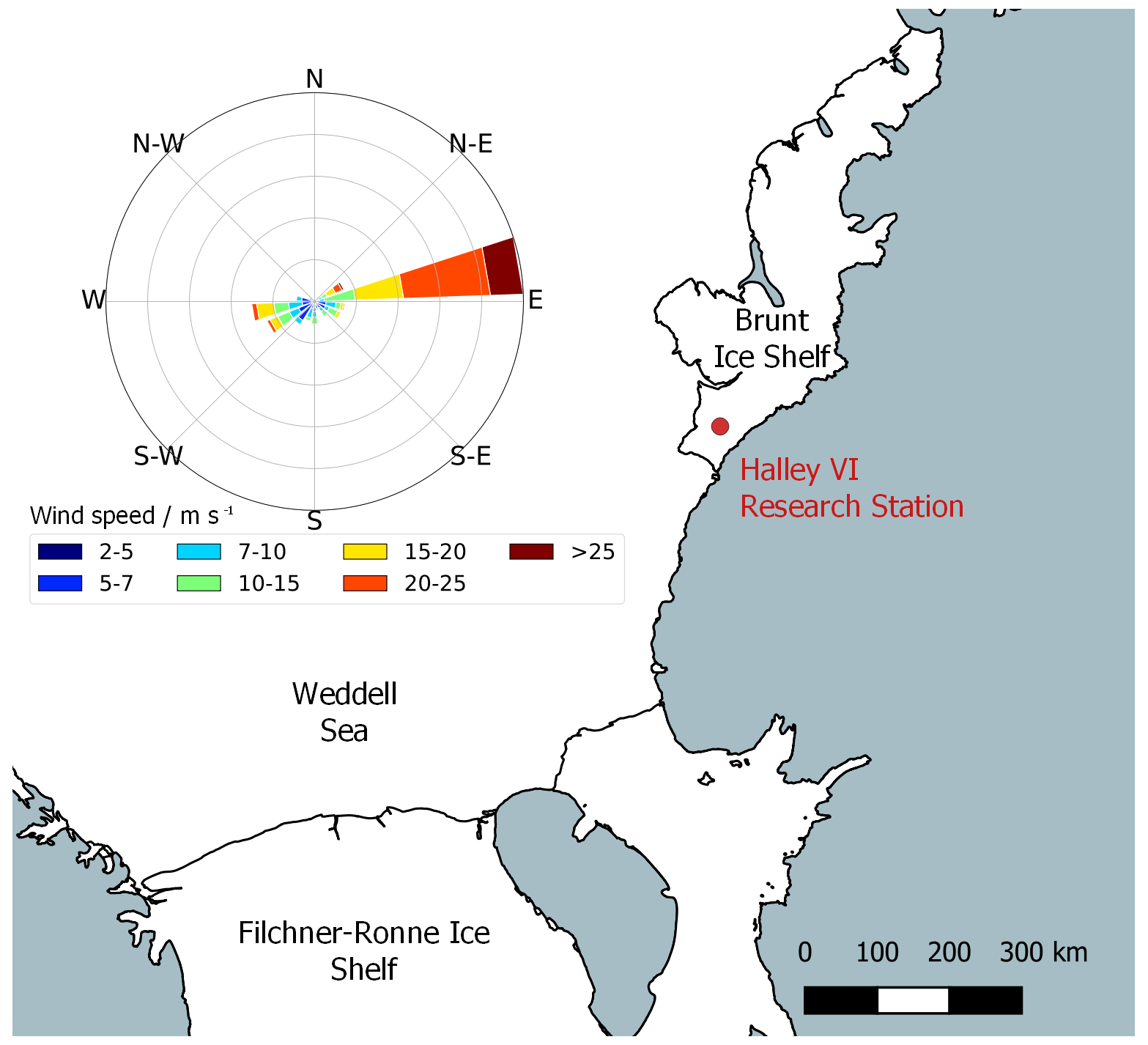
Figure 2A map showing the location of Halley on the Brunt Ice Shelf, Antarctica and a wind-rose plot for the period of the measurement campaign.
2.2 Methods
HONO was detected using a long-path absorption photometer (LOPAP; QUMA Elektronik & Analytik GmbH) which has been described in detail elsewhere (Heland et al., 2001; Kleffmann et al., 2002). Briefly, the instrument works by first collecting HONO in a stripping coil, housed in a temperature-controlled external sampling unit, by a fast chemical reaction in an acidic (pH of 0) sulfanilamide solution (reagent 1, 1 g L−1, lower than originally proposed; see von der Heyden et al., 2022). HONO is initially converted into NO+ which forms a diazonium salt by reaction with sulfanilamide. Due to the fast chemical reaction, much shorter gas–liquid contact times are applied (four-ring coil) compared to other wet-chemical HONO instruments (typically ≥10-ring coils), which require physical solubility equilibrium. This approach minimises sampling of interferences. In addition, the acidic sampling conditions slow down most known interfering reactions, which are faster under the neutral to alkaline conditions typically used in other wet-chemical instruments (Kleffmann and Wiesen, 2008). The solution is then pumped via a 3 m long temperature-controlled reagent line to the main instrument, in which an azo dye is formed by reaction with a 0.1 g L−1 N-(1-naphthyl)-ethylenediamine dihydrochloride (NED) solution (reagent 2). The dye is detected in long-path absorption tubing (path length of 5 m) by a spectrometer (Ocean Optics SD2000) at 550 nm. The dye concentration can be related to the atmospheric HONO amount fraction by carrying out calibrations with nitrite solutions of known concentrations and knowing the sample air-to-liquid flow rate ratio.
The sampling unit is made up of two stripping coils in series such that HONO and some interferences are taken up in the first coil, followed by only interferences in the second. The interferences are assumed to be taken up to the same small extent in both channels so that the HONO amount fraction can be calculated by subtracting the signal in channel 2 from that in channel 1 (Heland et al., 2001). The instrument has been studied for the effect of various possible interfering species, including NO, NO2, O3, peroxyacetyl nitrate (PAN), HNO3, and even more complex mixtures of volatile organic compounds (VOCs) and NOx in diesel engine exhaust fumes (Heland et al., 2001; Kleffmann et al., 2002). The instrument gave good agreement with the differential optical absorption spectroscopy (DOAS) technique under complex urban and smog chamber conditions (Kleffmann et al., 2006). However, comparison of the instrument under pristine polar conditions is still an open issue. In the present study, the average interference was 40 % of the channel 1 signal, highlighting the importance of using a two-channel instrument, in excellent agreement with other studies of LOPAP instruments under polar conditions and at high mountain sites (Kleffmann and Wiesen, 2008; Villena et al., 2011).
During the campaign, the LOPAP was calibrated every 5 d using nitrite solutions of known concentration ( and mg L−1). To maximise the instrument sensitivity, the gas-to-liquid flow rate ratio was optimised: the gas flow rate was set to 2 L min−1 (298 K, 1 atm) with the internal mass flow controller and checked frequently using a flow meter (DryCal DC-Lite), and the liquid flow rate through the stripping coil for each channel was regularly measured volumetrically and was between 0.15 and 0.18 mL min−1 during the measurement period. Baseline measurements were made every 6 h using a flow of pure nitrogen (99.998 %; BOC) at the instrument inlet. The detection limit (3σblank) was 0.26 pmol mol−1 for the measurement period. The average response time (90 % of final signal change) was (8 ± 1.5) min.
The LOPAP sampling unit required adaptation for use in cold polar environments. The sampling unit box and the reagent lines between this and the main instrument have been coated in Armaflex insulation: no HONO emission from such insulation materials has been detected (Kerbrat et al., 2012). The stripping coil and tubing to the sampling unit are temperature-controlled by a flow from a water bath (Thermo Haake K10 with DC10 circulator). The temperature of the sampling unit was kept at +18 ∘C.
The instrument's external sampling unit was mounted 0.4 m above the snow, 2.4 m from the container entrance, and pointed into the dominant wind direction (east). For most of the campaign, the sampling unit was stationary, except for a period of 12 h between 15:00 on 31 January and 03:00 on 1 February 2022 when the height was changed in regular intervals between 0.24 and 1.26 m above the snow in order to measure the HONO gradients needed to estimate vertical fluxes. An automatic elevator, built in-house, was used to raise and lower the sampling unit every 15 min (travel time of 1 min), meaning there was no human involvement in moving the sampling unit, and no tubing was needed to sample at different heights. Such tubing provides an artificial surface for HONO formation (Villena et al., 2011). The elevator is depicted in Fig. 3. The LOPAP data were shifted to account for the time delay ((17 ± 2) min) between gas intake and the observed absorption signal. This is determined from the average of all abrupt concentration changes (start/stop of blanks) and defined as the time between concentration change and the 50 % response of the instrument.

Figure 3An image of the elevator used to raise and lower the LOPAP sampling unit in order to estimate the air–snow HONO flux density using the flux-gradient method.
2.3 Ancillary measurements
The surface ozone amount fraction was measured simultaneously from the CAS lab by UV absorption (Thermo Scientific Model 49i Ozone Analyzer). Data were collected at a 10 s interval, quality controlled, and then averaged to 1 min for this analysis. Instrument limit of detection (LOD) was taken to be 3σ of 2 h of 10 s measurements of zero air. This was calculated to be 0.38 nmol mol−1. The analyser inlet pointed east and was located at 8 m above the snow surface.
For the HONO flux density calculation the wind speed and direction was measured with a 2D sonic anemometer (Gill Wind Observer 70) located 1.5 m south of the sampling unit and 1 m above the snow. The temperature gradient was measured with two thermometers (TME Ethernet Thermometer) mounted on the vertical post of the elevator at 0.05 and 1.26 m above the snow surface. During the campaign, the incoming shortwave solar radiation (300–2800 nm) was measured by a net radiometer (Kipp & Zonen; CNR4) located at the main station (1.5 km from the HONO sampling site). The ozone column density was measured with a Dobson spectrophotometer also at the main station.
Surface snow samples were collected from the top 3 cm of snow in the clean air sector on 6, 25, and 31 January 2022. The samples were collected using clean sampling procedures (wearing clean room suits, gloves, and masks) and transferred into 50 mL polypropylene tubes with screw caps (Corning CentriStar), which had been rinsed with UHP water and dried in a class 100 clean laboratory in Cambridge prior to field deployment. The samples were transported back to the UK at −20 ∘C where they were melted and analysed for major ions including nitrate using Dionex Integrion ICS-4000 ion chromatography systems with reagent-free eluent generation. A Dionex AS-AP autosampler was used to supply sample water to 250 µL sample loops on the cation and anion instruments. Anion analyses were performed using a Dionex Ionpac AG17-C (2 µm, 2×50 mm) guard column and AS17-C (2×250 mm) separator column. A 3.5–27 mM potassium hydroxide eluent concentration gradient was used for effective separation of the analytes. Calibration was achieved using a range of calibration standards prepared from Sigma-Aldrich standards (1000 µg g−1) by a series of gravimetric dilutions. Measurement accuracy was evaluated using European reference materials ERM-CA408 (simulated rainwater) and CA616 (groundwater) which were all within 5 %. The LOD was 2 ng g−1.
2.4 Flux calculations
The flux-gradient method was used to determine the HONO flux density following a similar approach as done previously for NOx in Antarctica (Jones et al., 2001; Frey et al., 2013). By measuring the HONO amount fraction at two heights, the concentration gradient can be found and is related to the flux density by
for which Kc is the turbulent diffusion coefficient (in m2 s−1) of a chemical tracer. In the atmospheric boundary layer, Kc may be approximated by the eddy diffusion coefficient for heat, Kh (Jacobson, 2005). It should be noted that a negative gradient in amount fraction will result in a positive flux density, equivalent to emission from the snow.
Monin–Obukhov similarity theory (MOST) is used to parameterise fluxes in the surface layer, about 10 % of the depth of the atmospheric boundary layer (Stull, 1988), where turbulent fluxes are assumed to be independent of height. The flux density can be calculated by
where κ is the von Karman constant (set to 0.4); u* is the friction wind velocity, found from wind speed measurements; and c(z) is the HONO amount fraction at height z. is the integrated stability function for heat, a function of where L is the Obukhov length. The full derivation of Eq. (2) is in Appendix A.
The application of MOST requires certain conditions to be met (Frey et al., 2013): (a) the flux density is constant between the two measurement heights, (b) the lower inlet height is above the surface roughness length, (c) the upper measurement height is within the surface layer, and (d) the measurement heights is far enough apart for the detection of a significant difference in amount fraction.
For (a), the chemical lifetime (τchem) with respect to photolytic loss was compared to the transport time (τtrans) between the two measurement heights. If τchem is much larger than τtrans, then the flux density can be assumed to be constant. τchem found from the inverse of the photolysis rate coefficient, J(HONO), was between 10 and 80 min. The transport time can be estimated by (Jacobson, 2005)
The transport time between 0.24 and 1.26 m above the snow for the flux measurement period at Halley was between 16 and 29 s. In all cases, the lifetime was significantly longer than the transport time, meaning the flux density can be assumed to be constant between the two heights.
The lower measurement height was 0.24 m, which is significantly above the surface roughness length of (5.6 ± 0.6) m measured previously at Halley (King and Anderson, 1994).
During the Antarctic summer, the boundary layer height at Halley is regularly stable, making it difficult to define (Anderson and Neff, 2008). Previous analysis of sodar (sound detection and ranging) measurements has suggested that the boundary layer at Halley in summer is consistently above 40 m (Jones et al., 2008). The equations of both Pollard et al. (1973) and Zilitinkevich and Baklanov (2002) have been used to estimate the mixing height at Antarctic locations (South Pole – Neff et al., 2008; Dome C – Frey et al., 2013). Though they are unlikely to predict the height accurately, these equations can provide a useful estimate of the minimum boundary layer height. For the period in question, this is calculated to be 75 and 95 m (Pollard et al., 1973, and Zilitinkevich and Baklanov, 2002, respectively). When temperature profiles recorded by daily weather balloon launches during the measurement campaign show a temperature inversion (Stull, 1988), this was above 100 m. Therefore, the upper measurement height, 1.26 m, was very likely within the surface layer.
A t test confirmed that the amount fraction difference between the two heights (Δy) was significant (p<0.01).
All of the above criteria were satisfied for the measurement period, so MOST was used to calculate the flux density by the method described above.
2.5 Photolysis rates
The rate coefficient of photochemical reactions can be calculated from
where σ and φ are the absorption cross-section and quantum yield for the photolysis reaction of interest, functions of wavelength (λ), and temperature (T). F is the actinic flux derived from the TUV radiation model over the wavelength range 300 to 1200 nm using measured ozone column density, a surface albedo of 0.95, and assuming clear-sky conditions (Madronich and Flocke, 1999; Lee-Taylor and Madronich, 2002). The calculated J values were then scaled by the ratio of measured and modelled incoming shortwave solar radiation to account for non-clear-sky conditions (see Fig. 4). It is noted that the wavelength ranges of modelled and measured radiation are not exactly the same, but the contribution of wavelengths >1200 nm is expected to be small.
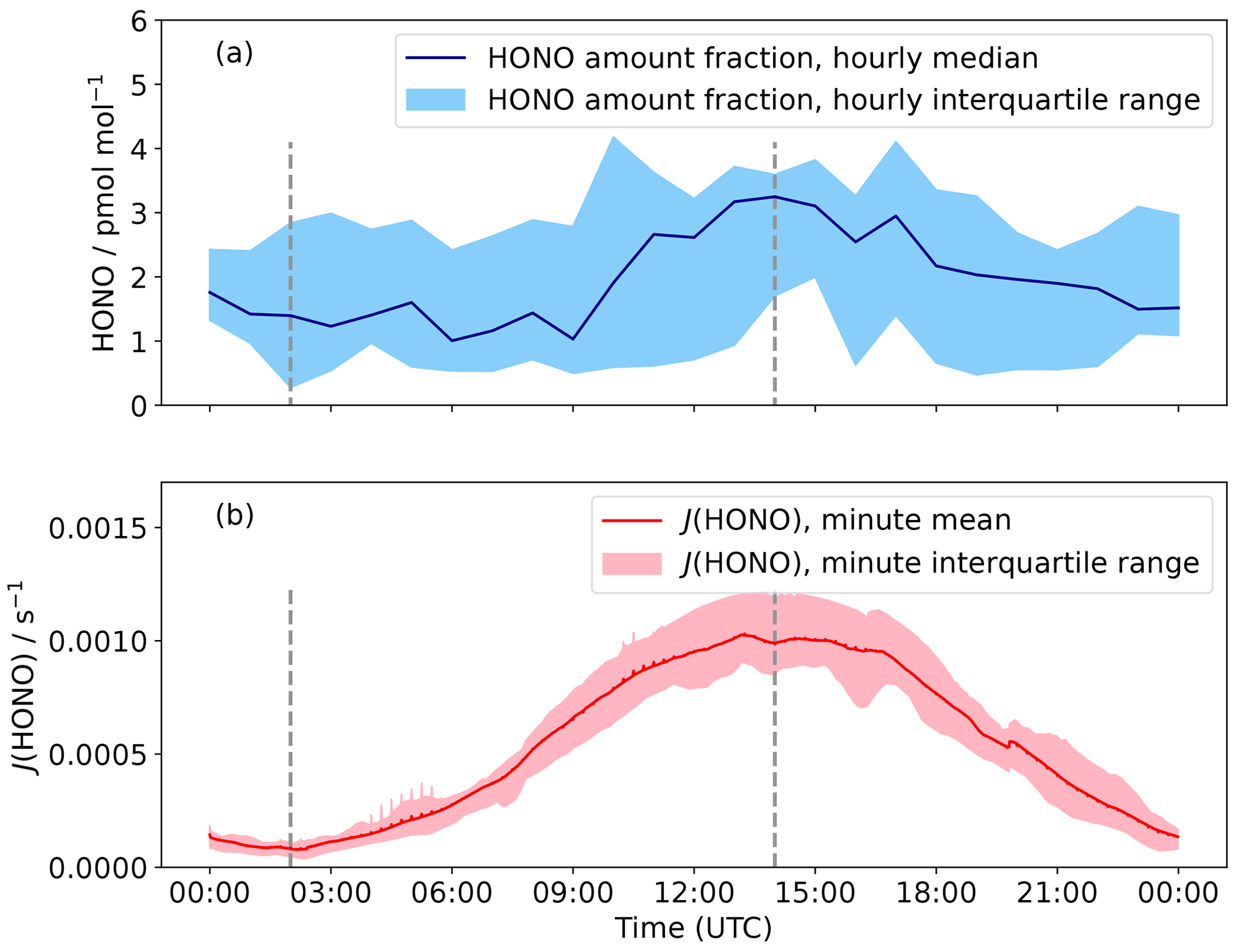
Figure 4(a) Hourly median diurnal cycle in HONO amount fraction for 22 January to 3 February 2022. The shaded region is the hourly interquartile range and the dashed grey lines are solar midnight and noon (02:00 and 14:00 UTC respectively). (b) J(HONO) was calculated by the TUV radiation model and then scaled to incoming solar radiation; again, the interquartile range is the shaded region.
3.1 HONO amount fraction
HONO amount fractions measured at Halley were between <0.3 and 14 pmol mol−1 (Fig. 5), with a mean of 2.1 pmol mol−1 (Bond et al., 2023).
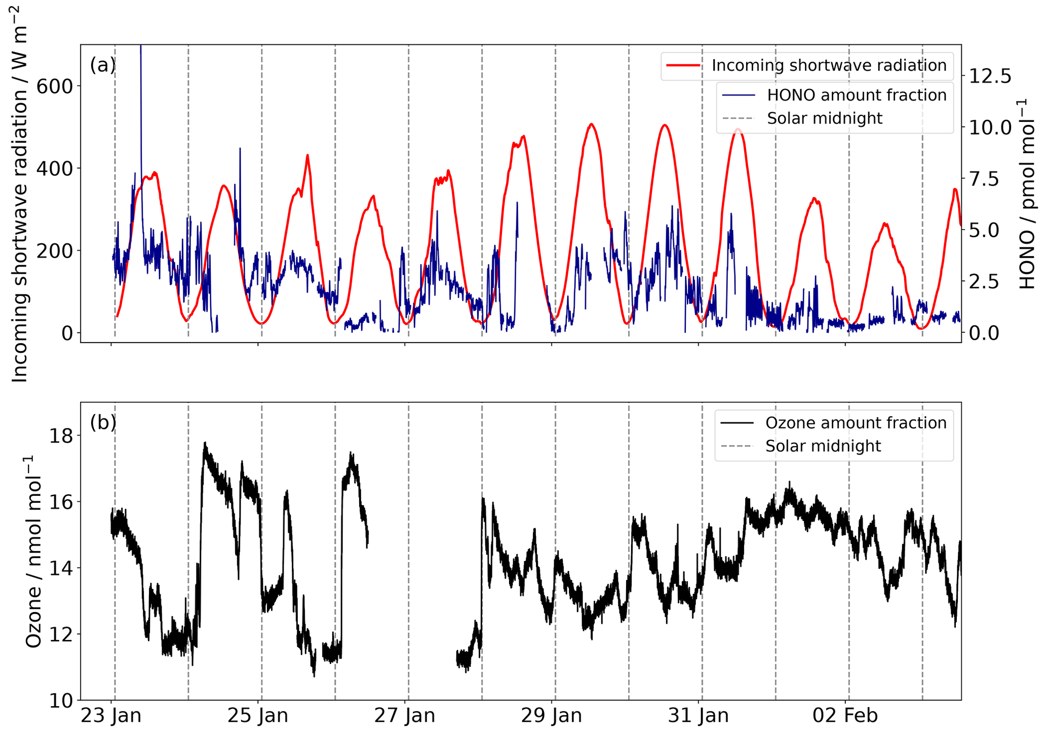
Figure 5(a) The HONO amount fraction at 1 min resolution recorded at Halley between 22 January and 3 February 2022, and incoming shortwave radiation between 300 and 2800 nm. The dashed lines are solar midnight (02:00 UTC). (b) The surface ozone amount fraction.
These HONO amount fractions are some of the lowest ever observed in Antarctica (see Table 1) and are only the second series of HONO observations at an Antarctic coastal ice-shelf location. When measurements were attempted once before at Halley, it was thought that the HONO amount fractions were overestimated (Clemitshaw, 2006; Jones et al., 2011). The HONO data collected in this study support this suggestion, as the mean is 2.1 pmol mol−1 compared with around 7 pmol mol−1 measured in January–February 2005 (Bloss et al., 2010). During this measurement period the average interference was 40 % of the channel 1 value, and occasionally >100 %, showing that HONO would be significantly overestimated without the two-channel sampling unit of the LOPAP.
Bloss et al. (2010)Kerbrat et al. (2012)Beine et al. (2006)Dibb et al. (2004)Liao et al. (2006)Legrand et al. (2014)Table 1Previous summertime measurements of atmospheric HONO amount fractions (y) in Antarctica.
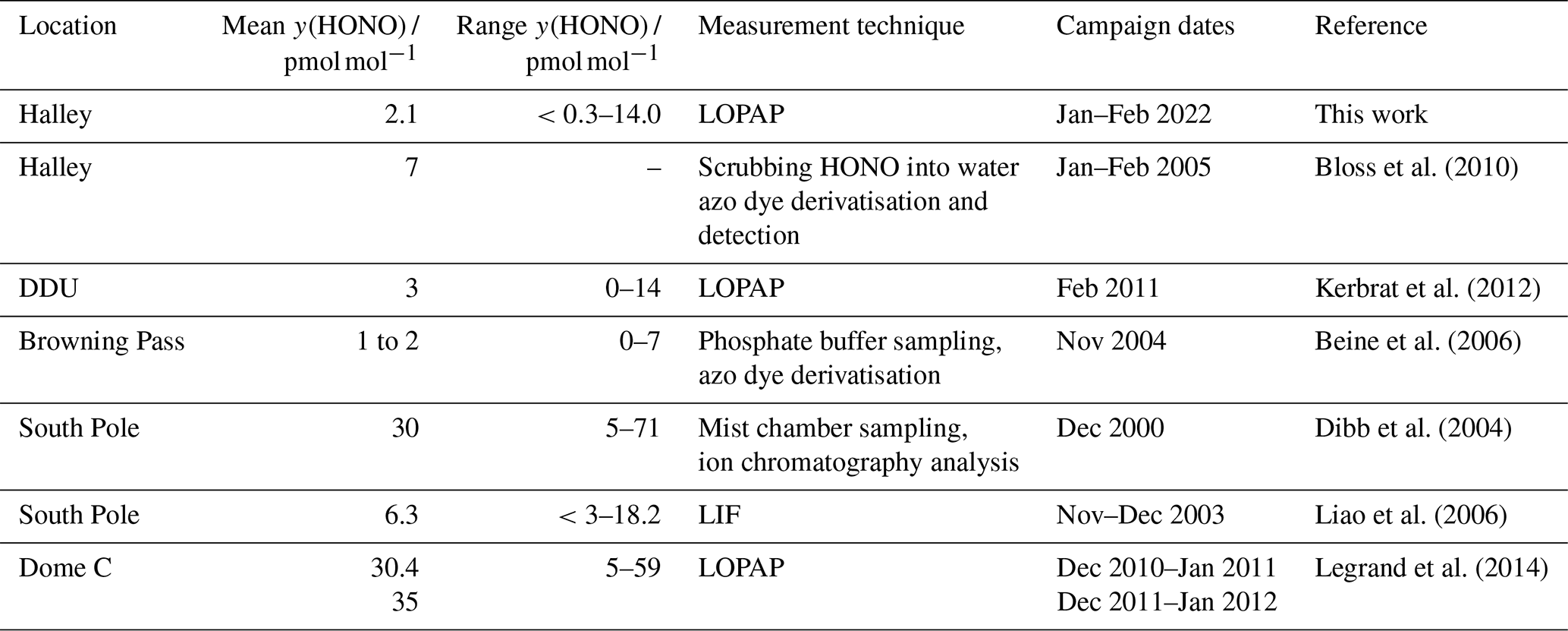
At other coastal sites, the HONO amount fractions are close to those seen in this study. At Browning Pass (Fig. 1), HONO amount fractions were <5 pmol mol−1, though the site conditions are unlike Halley, since the snow composition and pH may be affected by rock outcrops nearby (Beine et al., 2006). Small amount fractions were also observed at Dumont D'Urville (DDU), but this was attributed to the fact the site had no snow cover (Kerbrat et al., 2012). Higher amount fractions were observed in continental air masses, likely due to emissions from the snowpack on the continent.
HONO amount fractions at inland Antarctic locations are predominantly higher than those seen at Halley. At the South Pole, mean HONO amount fractions of 6.3 pmol mol−1 were measured by LIF (Liao et al., 2006). Dome C HONO amount fractions, measured using a LOPAP, were found to be higher than in most other studies (mean ca. 30 pmol mol−1) (Legrand et al., 2014). The higher HONO and NOx amount fractions can be explained by specific conditions on the high Plateau during summer, which include 24 h sunlight, a shallow and frequently stable boundary layer, and very low temperatures (King et al., 2006) leading to low primary production rates for HOx radicals (Davis et al., 2008). This causes a non-linear HOx–NOx chemical regime where the NOx lifetime increases with increasing NOx as proposed previously (Davis et al., 2008; Neff et al., 2018). Together, these factors support increased air–snow recycling and the accumulation of NOy in the regional boundary layer.
An interference of HNO4 in the LOPAP has been suggested (Kerbrat et al., 2012; Legrand et al., 2014). The LOPAP's response to HNO4 has been investigated in both the laboratory with an HNO4 source and in the field at Dome C by placing a heated tube at the instrument inlet to decompose HNO4. Both showed that the LOPAP partially measures HNO4 as HONO with approximately 100 pmol mol−1 HNO4 leading to a HONO interference of 15 pmol mol−1, but further investigation is needed to systematically quantify this effect (Legrand et al., 2014). In any case, Dome C is expected to have a much higher HNO4 amount fraction than Halley due to the fact its lifetime is controlled by thermal decomposition:
The rate coefficients for thermal decomposition of HNO4 are in Table 2. An average HNO4 lifetime with respect to thermal decomposition of 12 min was calculated from at Halley. This can be compared to an average lifetime of 21 h during January 2012 at Dome C (mean temperature of −31 ∘C). As a further check on this interference, the steady-state concentration of HNO4 at Halley was calculated. The method for this is detailed in Appendix B; the concentrations of HO2, NO2 and OH from the CHABLIS campaign were used. The average steady-state amount fraction was 0.05 pmol mol−1. Using the estimate of Legrand et al. (2014), this suggests that the interference is likely <0.01 pmol mol−1, well below the detection limit of the LOPAP.
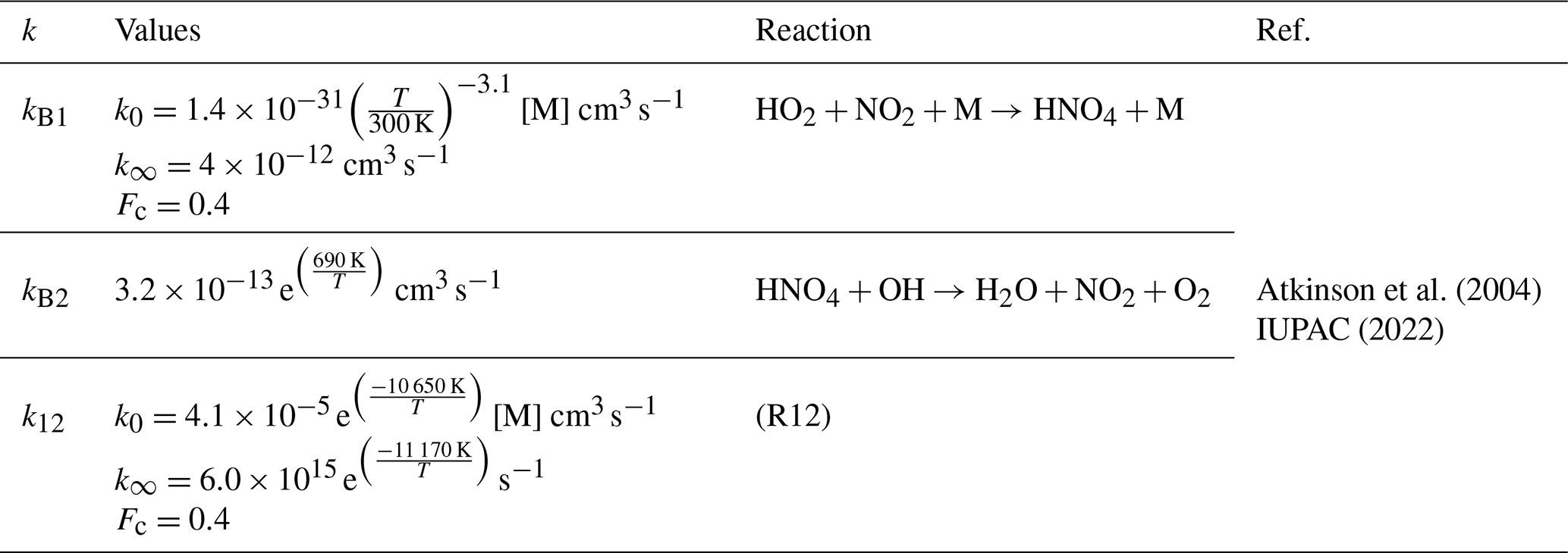
Atkinson et al. (2004)IUPAC (2022)Kleffmann et al. (2003)Table 2Rate coefficients used in calculations. Rate coefficients k4 and k12 are for pressure-dependent reactions with low- and high-pressure limit-rate coefficients k0 and k∞, respectively, [M] is the number concentration of air (cm−3), and Fc is the broadening factor.
The median diurnal cycle of HONO amount fraction shows a maximum at solar noon (Fig. 4), with a peak-to-peak amplitude of 2 pmol mol−1. Previous observations of HONO at Halley also showed a diurnal cycle but with a larger day-to-night variation (Clemitshaw, 2006), which is likely an overestimate of the true variation in HONO amount fractions. The diurnal cycle observed at Browning Pass compares well with that observed here: the maximum variation was 1 pmol mol−1 (Beine et al., 2006). The diurnal cycle of HONO amount fraction at Dome C showed a double peak due to the presence of a strong diurnal cycle in the boundary layer height; the amount fraction dipped at midday when the boundary layer height showed a strong increase (Legrand et al., 2014). The boundary layer height at Halley does not show such a diurnal pattern (King et al., 2006), so the variation is predominantly caused by the photochemical production of HONO peaking at solar noon.
3.2 HONO flux density
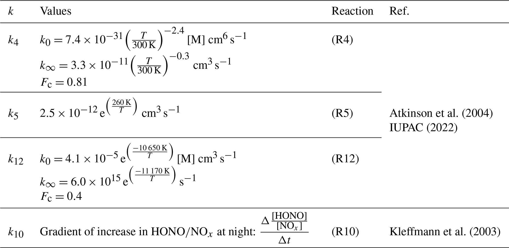
The measured flux density is plotted in Fig. 6 with the data needed for its calculation: the wind speed and temperature used to find the turbulent diffusion coefficient for heat (Kh) and the measured amount fraction gradient. The HONO amount fraction gradient is steep: the amount fraction decreases by about half between 0.24 and 1.26 m above the snow. The flux density varies between 0.5 and 3.4×10¹² from the snow surface, mainly driven by the amount fraction gradient, and appears to decrease between solar noon at 14:00 UTC and solar midnight at 02:00 UTC, suggesting a photochemical snowpack source. In the Antarctic, HONO fluxes have previously only been measured at Browning Pass, where larger values were found (mean upwards flux density of 4.8×10¹² ). However, occasionally the flux was downwards, equivalent to deposition. This is likely caused by the atypical snow composition: the snow is only weakly acidic and occasionally alkaline (Beine et al., 2006). More HONO flux measurements are available from the Arctic: flux densities up to 1014 from the snow have been observed (Zhou et al., 2001; Amoroso et al., 2010). However, these Arctic sites are more polluted and therefore there are more HONO precursors in the snow (NO2, nitrate, organics). Legrand et al. (2014) used measurements of the NOx flux density at Dome C and the HONO to NOx production rate ratio measured in a snow photolysis experiment in the laboratory to estimate a HONO emission flux density between 5 and 8×10¹² , larger than that observed here, likely due to the higher snow nitrate concentrations at Dome C.
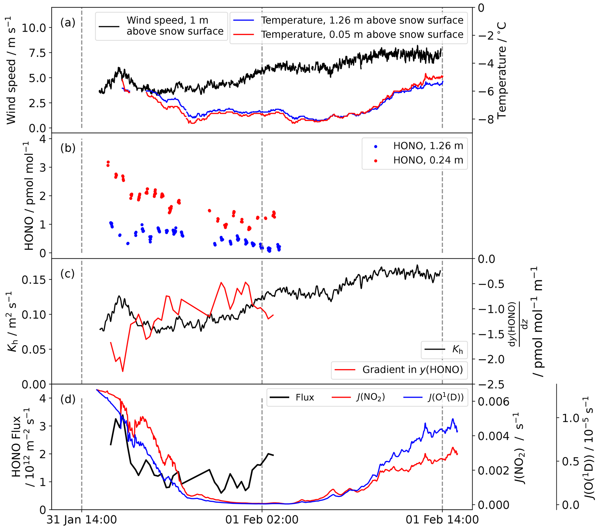
Figure 6(a) The wind speed and temperature recorded at Halley between 31 January and 1 February 2022. (b) The HONO amount fraction measured at 1.26 and 0.24 m above the snow surface. (c) The turbulent diffusion coefficient Kh and the amount fraction gradient calculated from the HONO amount fraction measurements at two heights (note that a negative gradient corresponds to emission of HONO from the snow). (d) The flux density calculated by combining Kh and the amount fraction gradient. The diurnal cycles in J(NO2) and J(O(1D)) calculated by the TUV radiation model, scaled to incident radiation, are also plotted.
4.1 HONO formation mechanisms
HONO formation in the snowpack, driving the flux to the boundary layer above, is typically attributed to nitrate photolysis. A HONO flux density from this reaction can be compared to that measured in this study to determine the source of HONO. The production rate (per area) above snow of reactive nitrogen from snow nitrate photolysis, Psnow(NOy), can be estimated using the following equation:
where is the nitrate photolysis rate coefficient, a function of depth in the snow pack, z. This can be approximated by (Chan et al., 2015), where is the photolysis rate coefficient at the snow surface. The e-folding depth (ze) is between 3.7 and 10 cm (7 cm is used here; Jones et al., 2011). is the nitrate number concentration (in units of cm−3). To derive HONO production from nitrate photolysis, a HONO yield coefficient Y(HONO) is included (Chen et al., 2019), and we also explicitly show the conversion from nitrate mass fraction to number concentration:
is the snow nitrate mass concentration (mass per mass of snow); ρsnow is the snow density, taken as 0.3 g cm−3 (Dominé et al., 2008); NA is Avogadro's number; and is the nitrate molar mass. was found from Eq. (4) using absorption cross-sections and quantum yields for ice (Chu and Anastasio, 2003), and it is s−1 at noon for the measurement period (assuming clear-sky conditions).
As detailed in Sect. 2.3, the surface snow nitrate mass fraction was measured, the mean value is (78.2 ± 18) ng g−1. A yield of 100 % gives a HONO production rate of 1.9×10¹² at a light intensity corresponding to local noon, below the maximum measured flux density of 3.4×10¹² . However, the yield is unlikely to be as high as 100 %.
There are two product channels for nitrate photolysis (Reactions R6 and R8); if it is assumed that all nitrite produced in Reaction (R6) is converted to HONO, Y(HONO) would be 10 % because Reaction (R8) dominates over Reaction (R6) by a factor of 9 (Chu and Anastasio, 2003). This gives a noon HONO production rate of only (0.19 ± 0.13) ×1012 . This is lower than the measured flux density (see Fig. 7). However, it has been suggested that the rate of nitrite production from nitrate photolysis could be as high as that of NO2 (Benedict and Anastasio, 2017; Benedict et al., 2017) implying Y(HONO) is greater than 10 %. Furthermore, the HONO yield from nitrate photolysis may also include a contribution from NO2 reacting on photosensitised organics (Reaction R11), and to a lesser extent from NO2 disproportionation (Reaction R9), which would further increase Y(HONO) and bring the HONO production rate from nitrate photolysis closer to the measured flux density. As well as the stated uncertainties in ze and , there is uncertainty in the quantum yield for nitrate photolysis in snow: an error of 50 % has been calculated from Chu and Anastasio (2003). These uncertainties are represented by the red shading in Fig. 7.
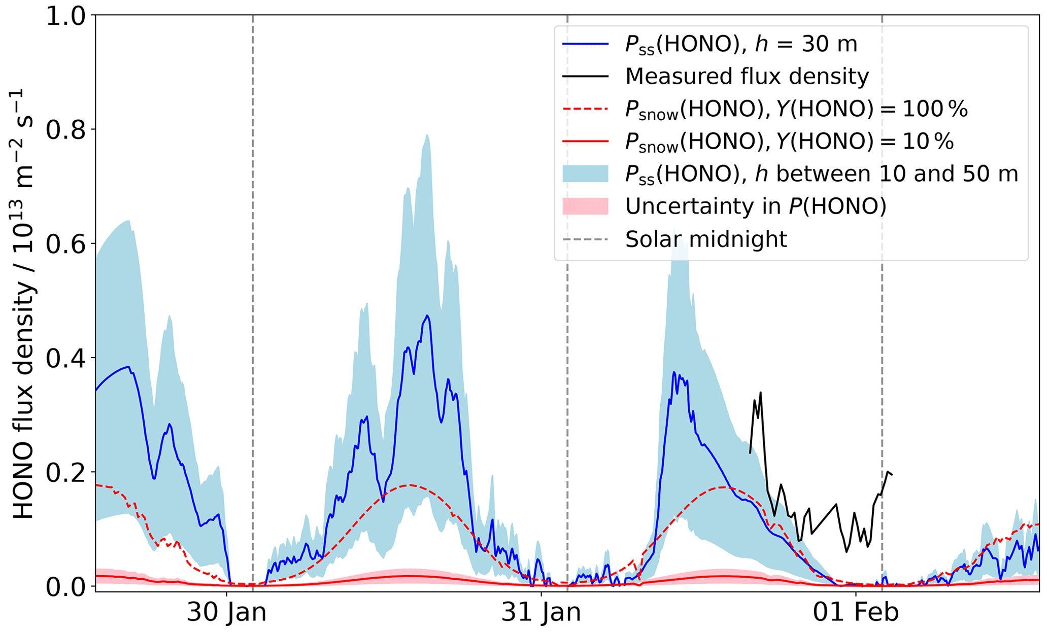
Figure 7HONO production calculated from Eq. (8), Pss(HONO). The blue-filled region is the production expected for mixing heights of 10 and 50 m. The HONO production from snow nitrate photolysis, Psnow(HONO), is plotted assuming a HONO yield of 100 % and 10 %. The uncertainty in this, from ze, and the photolysis quantum yield, is represented by the red-filled region. The measured flux density is also plotted. The production of HONO through reaction of OH+NO (Reaction R4) is not shown as its contribution would be <1011 .
Other assumptions made when carrying out this calculation include that the light attenuation in snow is exponential and that the snow density is 0.3 g cm−3, with a nitrate mass fraction that does not change with depth in the snow pack. It has also been assumed that all HONO produced will be released from the snow immediately; snowpack-produced HONO can be vented via wind pumping from the open snow pore space into the air above (Liao and Tan, 2008). The largest gradient in HONO amount fraction with height observed occurs during a wind speed increase (see Fig. 6) suggesting such wind pumping does occur at Halley. The degree of wind pumping will be affected by snow permeability, which is related to snow porosity (Waddington et al., 1996). During this measurement period, the snow was fresh and therefore more porous and likely more permeable than aged snow.
Photochemical reaction of NO2 on organic surfaces in the snow is a commonly suggested HONO formation mechanism (Reactions R10 and R11; Ammann et al., 2005; George et al., 2005). There is likely to be significant photosensitised organic matter present in the snow at Halley. Calace et al. (2005) found fulvic acid mass concentrations between 16 and 400 µg L−1 in coastal snow in east Antarctica, and Antony et al. (2011) found the total organic carbon (TOC) concentration of surface snow was 88 to 928 µg L−1 along a transect to the coast in east Antarctica with the higher values measured nearer the coast, which they attributed to marine sources associated with sea spray. Legrand et al. (2013) have highlighted that these studies could overestimate the organic matter content due to their sampling method and measurement technique. They suggest that the organic matter at coastal Antarctic sites could be lower, comparable to inland sites like Dome C (3–8 µg L−1). Legrand et al. (2014) suggest that this could still lead to significant HONO production. Assuming Dome C and Halley snow have similar organic content, a HONO flux density can be estimated based on the HONO:NOx emission ratio measured in a laboratory study of Dome C snow (Legrand et al., 2014) and the measured NOx flux density at Halley (Bauguitte et al., 2012). The HONO:NOx ratio is temperature dependent: the highest temperature studied by Legrand et al. (2014) is −13 ∘C, which is below the Halley air temperature for the flux measurement period. An emission ratio of 0.77 and NOx flux density of 7.3×10¹² give a HONO flux density of 5.6×10¹² , close to the measured value. NO2 has been measured previously at Halley (see Table 3): amount fractions were lower than at other sites, regularly <10 pmol mol−1, which would limit HONO production via this mechanism. However, in interstitial air in snow blocks at Neumayer station (a similar coastal ice-shelf location), NO2 amount fractions were found to be higher than in ambient air, up to 40 pmol mol−1 (Jones et al., 2000). In their laboratory study of this HONO production mechanism, Bartels-Rausch et al. (2010) estimate that such an NO2 amount fraction, with a snow TOC concentration of 10 to 1000 µg L−1, would lead to a flux density of 3×10¹² to 4×10¹² . This estimate agrees well with the measured HONO flux density from the snow at Halley, provided that all HONO produced is also emitted into the atmosphere. To investigate this possible source further the snowpack must be analysed in more detail for the presence of such photosensitised species.
Bloss et al. (2007)Bauguitte et al. (2012)Table 3Observations of HOx concentrations and NOx amount fractions (y) made during the CHABLIS campaign at Halley (January–February 2005) and the temperature (θ) and atmospheric pressure (patm) observed during this campaign (January–February 2022).

4.2 Additional HONO source
In order to assess the consistency of the measured HONO amount fractions and flux density, a simple box model calculation was undertaken. The change in the atmospheric HONO amount fraction over time can be written as the sum of the main sources and sinks:
which takes into account the production of HONO from the snow (Pss(HONO)), as well as HONO formation through NO and OH combination (Reaction R4) and loss through reaction with OH (Reaction R5). This can be simplified as the rates of Reactions (R4) and (R5) are typically slow, especially under remote conditions, meaning that in this model, the HONO budget is dominated by emission of HONO from snow nitrate photolysis and atmospheric photolysis of HONO itself. Rearranging and simplifying Eq. (7) gives
For simplification, it is assumed that the emitted HONO is homogeneously mixed in a layer of height h. The boundary layer height at Halley can be hard to define (Anderson and Neff, 2008), but for the current measurement period, the boundary layer height is likely above 40 m (King et al., 2006; Jones et al., 2008). These calculated flux densities, for h between 10 and 50 m, reflect the shape of the measured flux density well showing peaks at noon, though the calculated flux densities appear to decrease to 0 at night, which the measurements do not (Fig. 7).
The assumption of a constant HONO amount fraction up to height h above the snow surface is the largest source of uncertainty in this simple box model. Steep gradients in HONO amount fraction are expected, caused by the ground surface source, the turbulent transport, and the photolytic loss of HONO in the atmosphere. The gradients were confirmed in the present study, for which the HONO amount fraction decreased to ca. half between 0.24 and 1.26 m height (see Fig. 6b). However, these gradients can only be described correctly by a 1D model approach, which is out of the scope of the present study. Errors in the flux density calculation caused by deviations from MOST are also a possibility, and this comparison is further limited by the flux density measurements only being possible for one 12 h period.
For completeness, we tried including reactions involving NO and OH (Reactions R4 and R5) in the simple box model represented by Eq. (7). Due to the lack of concurrent observations, previous measurements of other gases during the CHABLIS campaign in 2004 and 2005 at Halley (Jones et al., 2008) were used for further calculations. Specifically, OH and NO data for the days of January and February 2005 corresponding to the days in 2022 on which HONO was measured (22 January to 3 February) have been used here. NO amount fractions were low, with a mean of 5.7 pmol mol−1, but showed a diurnal cycle peaking between 19:00 and 20:00 UTC, 5 h after solar noon (14:00 UTC) (Bauguitte et al., 2012). The mean OH concentration was 3.9×105 cm−3 with an average noontime maximum of 7.9×105 cm−3 (Bloss et al., 2007). These data, along with other gases that were measured in the campaign, are summarised in Table 3. The reaction rate coefficients used in these calculations are summarised in Table 2. Using these NO and OH concentrations, a new value of Pss(HONO) was calculated. As expected, the inclusion of these reactions does not make a large difference; the flux density calculated by this method is on average 3 % smaller than that from Eq. (8), though it is also occasionally larger.
4.3 Photostationary-state HONO
If the flux density from the snow is ignored, the photostationary-state (PSS) HONO amount fraction can be calculated. This assumes HONO is solely formed in the air through Reaction (R4) and lost through Reactions (R1) and (R5).
Using NO and OH CHABLIS data again, an average photostationary-state HONO amount fraction of 0.07 pmol mol−1 was calculated. This showed a diurnal cycle with a maximum at solar noon and minimum at night. However, this calculation is only valid at the HONO measurement height of 0.4 m if it is assumed there are no gradients in the NO and OH amount fractions which were measured at higher altitudes, 4.5 to 6 m above the snow. HONO was found to have a steep amount fraction gradient, which suggests that by 4.5 to 6 m above the snow, the amount fraction could be close to the photostationary-state amount fraction.
The inclusion of HONO formation through a dark reaction of NO2 on surfaces (Reaction R10) (Ammann et al., 2005) in the PSS calculation raised the HONO amount fraction to 0.3 pmol mol−1, which is still significantly lower than that measured. For this reaction, s−1 was estimated from the nighttime increase in the HONO:NOx ratio in the average diurnal cycle observed at Halley (see Table 2) (Kleffmann et al., 2003). Clearly an additional source is required to raise the HONO amount fraction above stationary-state levels.
4.4 HONO:NOx ratio
The HONO:NOx amount fraction ratio can provide a check on the HONO data: under steady-state conditions of HONO and NOx sources and sinks, and assuming that all NOx is produced by HONO photolysis as an upper limit, the HONO:NOx ratio should approach that of their lifetimes (τ(HONO):τ(NOx)) (Villena et al., 2011).
Using the HONO data collected and the NOx amount fraction for the same time period in 2005 (Bauguitte et al., 2012), the ratio of the amount fractions was calculated. This is between 0.15 and 0.35 and shows no diurnal cycle. This is significantly lower than other studies (Beine et al., 2001, 2002; Dibb et al., 2002; Jones et al., 2011; Legrand et al., 2014), supporting that our measurements are comparatively free from interferences. Only during measurements in Utqiaġvik, Alaska (formerly Barrow, Alaska) were even lower HONO:NOx ratios of 0.06 observed, also using the LOPAP technique (Villena et al., 2011). However, the 2022 HONO measurements were made significantly closer to the snow surface than the 2005 NOx measurements (0.4 m compared to 6 m). The steep gradient in HONO that has been observed suggests that the HONO amount fraction at 6 m above the snow will be considerably lower. This would further reduce the ratio, which still supports that these measurements are relatively free from interferences.
The ratio of HONO to NOx lifetimes is 0.07 at night (80 min:19 h, τ(HONO) calculated for loss by photolysis and τ(NOx) for loss by reaction with OH; Seinfeld and Pandis, 1998). This is a factor of 2–4 lower than the measured HONO:NOx ratio. The daytime ratio of lifetimes (12 min:6 h; Bauguitte et al., 2012) is 0.03 and is even lower compared to the range measured because the HONO measurements were made close to the snow surface (the HONO source) where the steady-state conditions are not fulfilled. However, Bauguitte et al. (2012) found that the NOx lifetime was reduced by halogen processing (BrNO3 and INO3 formation and heterogeneous uptake). A reduced NOx lifetime would improve the agreement with the observed HONO:NOx ratio.
4.5 HONO as a source of OH
HONO photolysis is an OH source; when the measured HONO amount fraction is higher than the calculated photostationary-state amount fraction, HONO is a net source of the OH radical. The importance of this net source compared to that from ozone at Halley is plotted in Fig. 8.
Figure 8The contribution of HONO and ozone to the OH production rate at Halley. The average J(O(1D)) for Halley is also shown.
Table 4Maximum and average HOx production by primary HOx sources (HONO, O3, formaldehyde (HCHO) and hydrogen peroxide (H2O2)) and HOx recycling at different Antarctic (Halley and Dome C) and Arctic (Utqiaġvik) locations.

As part of the CHABLIS campaign, Bloss et al. (2007) calculated the contribution of various OH sources to the HOx budget at Halley. It was found that the halogen species contributed the most; Halley's coastal location means there are high halogen concentrations (Saiz-Lopez et al., 2007). The halogen species HOI and HOBr show a strong diurnal pattern and contribute up to 89 and 14 OH at solar noon respectively. The OH production by HOBr is comparable to that calculated for HONO from the measurements made here (Table 4). However, it must again be highlighted that the halogen measurements were made higher above the snow (4 to 5 m; Saiz-Lopez et al., 2008) than those of HONO and that the HONO OH source estimate is only valid at 0.4 m where the HONO was measured. At higher altitudes above the snow, HONO will approach the PSS amount fraction leading to a lower contribution to the OH radical source. Thus, the contribution of HONO to the OH radical initiation will be limited only to the lowest part of the mixing layer.
The surface ozone amount fraction recorded during this measurement period is comparable with that measured during the CHABLIS campaign (mean of 14 nmol mol−1 here, 10 nmol mol−1 during January 2005) and lower than at other Antarctic sites due to the high halogen concentrations. However, at the other sites in Table 4, HONO is a more important OH source than ozone. The low temperatures at these sites (mean: Utqiaġvik −26, DC −31 ∘C) mean the extremely dry air limits OH production via Reactions (R2) and (R3). At Halley, a warmer coastal location, the water vapour concentration is not limiting, and OH formation through ozone photolysis still dominates. Nevertheless, HONO photolysis as a source of OH cannot be discounted. The HONO amount fractions that were initially thought to be present at Halley, detected during the CHABLIS campaign (Bloss et al., 2010), would lead to an overestimation of the HOx budget (Bloss et al., 2007). Besides conceptional problems when comparing box model calculations with HONO measurements close to the snow surface, these HONO measurements should make the HOx budget at Halley easier to rationalise.
We have presented the first interference-free measurements of atmospheric HONO amount fractions at an Antarctic coastal ice-shelf location. The lower values we observed here may be at least partly due to interference correction by the two-channel LOPAP technique. Amount fractions were between <0.26 and 14 pmol mol−1, with a mean of 2.1 pmol mol−1, and exhibited a diurnal pattern peaking at noon. A HONO flux density of 0.5 to 3.4×10¹² from the snow was measured, which is close to the estimated HONO production from nitrate photolysis, suggesting this reaction is a driver of HONO release from the snow. The flux density required to reach the measured amount fraction, with known HONO sources and sinks, was calculated by a simplified box model and is comparable to that measured here. HONO is an important OH source at Halley: these measurements suggest that HONO could contribute up to 12 of OH, which should fit better with the HOx budget previously modelled (Bloss et al., 2007, 2010). However, such calculations were limited by the strong HONO gradients and by the height difference between the HONO measurements of this campaign and the HOx, NOx, and halogen species measurements of the CHABLIS campaign.
There is a clear need for a complete campaign covering HOx, NOx, NOy, and halogen species, with measurements at the same height, to understand the interaction of the snow surface and boundary layer above. The observation of a steep gradient in HONO amount fraction requires further investigation. A 1D model combining amount fractions and fluxes of such gases, as well as meteorological data, is crucial for forming a consistent picture of the importance of the snow in the composition of the air at different heights through the polar boundary layer.
As discussed in the main text, the flux-gradient method was used to determine the HONO flux density using Eq. (1):
where Kc, the turbulent diffusion coefficient for a chemical tracer, may be approximated by the eddy diffusion coefficient for heat, Kh (Jacobson, 2005). Using Monin–Obukhov similarity theory (MOST), Kh can be calculated via
where κ is the von Karman constant (set to 0.4), u* is the friction wind velocity, z is the height, and Φh the stability function for heat (Jacobson, 2005). Φh is empirically determined as a function of where L is the Obukhov length (King and Anderson, 1994).
where is the temperature, θ* is the potential temperature scale, and g is the gravitational constant. Combining Eqs. (1) and (A1) results in
which can be integrated to
This is the same as Eq. (2) in the main text. Therefore, to find the flux density, the amount fraction of the gas must be known at two heights, along with the integrated stability function and u*. Three-dimensional sonic anemometer measurements are normally used to find u* but were not available for this measurement period, so u* was first estimated for a neutral boundary layer according to (Anderson and Bauguitte, 2007)
where u(zr) is the wind speed measured at height zr, and z0 is the surface roughness length that has been measured previously at Halley, z0=(5.6 ± 0.5) m (King and Anderson, 1994). Forms of the integrated stability function have been established for stable and neutral conditions above snow. The value of provides an indication of the boundary layer conditions and hence the expression for the integrated stability function. L was estimated by Eq. (A2), which requires θ*. This was also initially estimated for a neutral boundary layer, using temperature measurements made at two heights (Jacobson, 2005):
In the case of the measurement period at Halley, the value of was found to be close to zero so the boundary layer was assumed to be neutral and the initial estimates of u* and θ* were valid. The integrated stability function for a neutral boundary layer is
where Prt is the turbulent Prandtl number with a value of 0.95 (King and Anderson, 1994). Combining this with Eq. (A4) gives
which was used to calculate the flux density.
The steady-state concentration of HNO4 was calculated using Eq. (B1). The reactions and their rate coefficients are listed in Table B1.
Table B1Rate coefficients used in calculation of the HNO4 steady-state concentration.
Loss of HNO4 via photolysis was also included in the calculation (). The rate coefficient, J(HNO4), was derived from the TUV radiation model as described in the main text.
The data are available at the UK Polar Data Centre: https://doi.org/10.5285/94b2f348-d6cc-4bcd-b921-5c0928ab3c2d (Bond et al., 2023).
Field measurements at Halley were carried out by AMHB with assistance from FAS. Data analysis was done by AMHB with supervision from MMF, JaK, JöK, and AEJ. AMHB wrote the first draft of the paper with contributions from all co-authors.
At least one of the (co-)authors is a member of the editorial board of Atmospheric Chemistry and Physics. The peer-review process was guided by an independent editor, and the authors also have no other competing interests to declare.
Publisher's note: Copernicus Publications remains neutral with regard to jurisdictional claims in published maps and institutional affiliations.
We thank the British Antarctic Survey Halley science team for their support provided during the field season, in particular Thomas Barningham and Jack Farr. We also thank BAS engineers Ross Sanders and Rad Sharma for designing and building the LOPAP elevator, and Jack Humby and Shaun Miller for their help with the IC analysis.
This work was supported by the Natural Environment Research Council and the ARIES Doctoral Training Partnership (grant no. NE/S007334/1). We thank the Collaborative Antarctic Science Scheme (CASS) for funding the fieldwork at Halley VI Research Station. Markus M. Frey, Anna E. Jones and Freya A. Squires were supported by core funding from the Natural Environment Research Council to the British Antarctic Survey's Atmosphere, Ice and Climate Program.
This paper was edited by Markus Ammann and reviewed by two anonymous referees.
Ammann, M., Rössler, E., Strekowski, R., and George, C.: Nitrogen dioxide multiphase chemistry: Uptake kinetics on aqueous solutions containing phenolic compounds, Phys. Chem. Chem. Phys., 7, 2513–2518, https://doi.org/10.1039/b501808k, 2005. a, b, c
Amoroso, A., Beine, H. J., Sparapani, R., Nardino, M., and Allegrini, I.: Observation of coinciding arctic boundary layer ozone depletion and snow surface emissions of nitrous acid, Atmos. Environ., 40, 1949–1956, https://doi.org/10.1016/j.atmosenv.2005.11.027, 2006. a
Amoroso, A., Dominé, F., Esposito, G., Morin, S., Savarino, J., Nardino, M., Montagnoli, M., Bonneville, J. M., Clement, J. C., Ianniello, A., and Beine, H. J.: Microorganisms in dry polar snow are involved in the exchanges of reactive nitrogen species with the atmosphere, Environ. Sci. Technol., 44, 714–719, https://doi.org/10.1021/es9027309, 2010. a
Anderson, P. S. and Bauguitte, S. J.-B.: Behaviour of tracer diffusion in simple atmospheric boundary layer models, Atmos. Chem. Phys., 7, 5147–5158, https://doi.org/10.5194/acp-7-5147-2007, 2007. a
Anderson, P. S. and Neff, W. D.: Boundary layer physics over snow and ice, Atmos. Chem. Phys., 8, 3563–3582, https://doi.org/10.5194/acp-8-3563-2008, 2008. a, b
Antony, R., Mahalinganathan, K., Thamban, M., and Nair, S.: Organic carbon in antarctic snow: Spatial trends and possible sources, Environ. Sci. Technol., 45, 9944–9950, https://doi.org/10.1021/es203512t, 2011. a
Atkinson, R., Baulch, D. L., Cox, R. A., Crowley, J. N., Hampson, R. F., Hynes, R. G., Jenkin, M. E., Rossi, M. J., and Troe, J.: Evaluated kinetic and photochemical data for atmospheric chemistry: Volume I – gas phase reactions of Ox, HOx, NOx and SOx species, Atmos. Chem. Phys., 4, 1461–1738, https://doi.org/10.5194/acp-4-1461-2004, 2004. a, b
Bartels-Rausch, Th., Brigante, M., Elshorbany, Y. F., Ammann, M., D'Anna, B., George, C., Stemmler, K., Ndour, M., and Kleffmann, J.: Humic acid in ice: Photo-enhanced conversion of nitrogen dioxide into nitrous acid, Atmos. Environ., 44, 5443–5450, https://doi.org/10.1016/j.atmosenv.2009.12.025, 2010. a, b
Bauguitte, S. J.-B., Bloss, W. J., Evans, M. J., Salmon, R. A., Anderson, P. S., Jones, A. E., Lee, J. D., Saiz-Lopez, A., Roscoe, H. K., Wolff, E. W., and Plane, J. M. C.: Summertime NOx measurements during the CHABLIS campaign: can source and sink estimates unravel observed diurnal cycles?, Atmos. Chem. Phys., 12, 989–1002, https://doi.org/10.5194/acp-12-989-2012, 2012. a, b, c, d, e, f
Beine, H., Colussi, A. J., Amoroso, A., Esposito, G., Montagnoli, M., and Hoffmann, M. R.: HONO emissions from snow surfaces, Environ. Res. Lett., 3, 045005, https://doi.org/10.1088/1748-9326/3/4/045005, 2008. a
Beine, H. J., Allegrini, I., Sparapani, R., Ianniello, A., and Valentini, F.: Three years of springtime trace gas and particle measurements at Ny-Ålesund, Svalbard, Atmos. Environ., 35, 3645–3658, https://doi.org/10.1016/S1352-2310(00)00529-X, 2001. a, b
Beine, H. J., Dominé, F., Simpson, W., Honrath, R. E., Sparapani, R., Zhou, X., and King, M.: Snow-pile and chamber experiments during the Polar Sunrise Experiment “Alert 2000”: Exploration of nitrogen chemistry, Atmos. Environ., 36, 2707–2719, https://doi.org/10.1016/S1352-2310(02)00120-6, 2002. a, b
Beine, H. J., Amoroso, A., Esposito, G., Sparapani, R., Ianniello, A., Georgiadis, T., Nardino, M., Bonasoni, P., Cristofanelli, P., and Dominé, F.: Deposition of atmospheric nitrous acid on alkaline snow surfaces, Geophys. Res. Lett., 32, L10808, https://doi.org/10.1029/2005GL022589, 2005. a
Beine, H. J., Amoroso, A., Dominé, F., King, M. D., Nardino, M., Ianniello, A., and France, J. L.: Surprisingly small HONO emissions from snow surfaces at Browning Pass, Antarctica, Atmos. Chem. Phys., 6, 2569–2580, https://doi.org/10.5194/acp-6-2569-2006, 2006. a, b, c, d, e, f, g
Benedict, K. B. and Anastasio, C.: Quantum Yields of Nitrite () from the Photolysis of Nitrate () in Ice at 313 nm, J. Phys. Chem. A, 121, 8474–8483, https://doi.org/10.1021/acs.jpca.7b08839, 2017. a
Benedict, K. B., McFall, A. S., and Anastasio, C.: Quantum Yield of Nitrite from the Photolysis of Aqueous Nitrate above 300 nm, Environ. Sci. Technol., 51, 4387–4395, https://doi.org/10.1021/acs.est.6b06370, 2017. a
Bloss, W. J., Lee, J. D., Heard, D. E., Salmon, R. A., Bauguitte, S. J.-B., Roscoe, H. K., and Jones, A. E.: Observations of OH and HO2 radicals in coastal Antarctica, Atmos. Chem. Phys., 7, 4171–4185, https://doi.org/10.5194/acp-7-4171-2007, 2007. a, b, c, d, e, f
Bloss, W. J., Camredon, M., Lee, J. D., Heard, D. E., Plane, J. M. C., Saiz-Lopez, A., Bauguitte, S. J.-B., Salmon, R. A., and Jones, A. E.: Coupling of HOx, NOx and halogen chemistry in the antarctic boundary layer, Atmos. Chem. Phys., 10, 10187–10209, https://doi.org/10.5194/acp-10-10187-2010, 2010. a, b, c, d, e, f
Bond, A., Squires, F., Frey, M., and Kaiser, J.: Atmospheric nitrous acid amount fraction at Halley in January and February 2022, Version 1.0, NERC EDS UK Polar Data Centre [data set], https://doi.org/https://doi.org/10.5285/94b2f348-d6cc-4bcd-b921-5c0928ab3c2d, 2023. a, b
Calace, N., Cantafora, E., Mirante, S., Petronio, B. M., and Pietroletti, M.: Transport and modification of humic substances present in Antarctic snow and ancient ice, J. Environ. Monitor., 7, 1320–1325, https://doi.org/10.1039/b507396k, 2005. a
Chan, H. G., King, M. D., and Frey, M. M.: The impact of parameterising light penetration into snow on the photochemical production of NOx and OH radicals in snow, Atmos. Chem. Phys., 15, 7913–7927, https://doi.org/10.5194/acp-15-7913-2015, 2015. a
Chen, Q., Edebeli, J., McNamara, S. M., Kulju, K. D., May, N. W., Bertman, S. B., Thanekar, S., Fuentes, J. D., and Pratt, K. A.: HONO, Particulate Nitrite, and Snow Nitrite at a Midlatitude Urban Site during Wintertime, ACS Earth and Space Chemistry, 3, 811–822, https://doi.org/10.1021/acsearthspacechem.9b00023, 2019. a, b
Chu, L. and Anastasio, C.: Quantum Yields of Hydroxyl Radical and Nitrogen Dioxide from the Photolysis of Nitrate on Ice, J. Phys. Chem. A, 107, 9594–9602, https://doi.org/10.1021/jp0349132, 2003. a, b, c
Clemitshaw, K. C.: Coupling between the Tropospheric Photochemistry of Nitrous Acid (HONO) and Nitric Acid (HNO3), Environ. Chem., 3, 31–34, https://doi.org/10.1071/EN05073, 2006. a, b
Davis, D. D., Seelig, J., Huey, G., Crawford, J., Chen, G., Wang, Y., Buhr, M., Helmig, D., Neff, W., Blake, D., Arimoto, R., and Eisele, F.: A reassessment of Antarctic plateau reactive nitrogen based on ANTCI 2003 airborne and ground based measurements, Atmos. Environ., 42, 2831–2848, https://doi.org/10.1016/j.atmosenv.2007.07.039, 2008. a, b, c
Dibb, J. E., Arsenault, M., Peterson, M. C., and Honrath, R. E.: Fast nitrogen oxide photochemistry in Summit, Greenland snow, Atmos. Environ., 36, 2501–2511, https://doi.org/10.1016/S1352-2310(02)00130-9, 2002. a, b, c
Dibb, J. E., Gregory Huey, L., Slusher, D. L., and Tanner, D. J.: Soluble reactive nitrogen oxides at South Pole during ISCAT 2000, Atmos. Environ., 38, 5399–5409, https://doi.org/10.1016/j.atmosenv.2003.01.001, 2004. a, b, c, d
Domine, F., Albert, M., Huthwelker, T., Jacobi, H.-W., Kokhanovsky, A. A., Lehning, M., Picard, G., and Simpson, W. R.: Snow physics as relevant to snow photochemistry, Atmos. Chem. Phys., 8, 171–208, https://doi.org/10.5194/acp-8-171-2008, 2008. a
Finlayson-Pitts, B. J., Wingen, L. M., Sumner, A. L., Syomin, D., and Ramazan, K. A.: The heterogeneous hydrolysis of NO2 in laboratory systems and in outdoor and indoor atmospheres: An integrated mechanism, Phys. Chem. Chem. Phys., 5, 223–242, https://doi.org/10.1039/b208564j, 2003. a
Frey, M. M., Stewart, R. W., McConnell, J. R., and Bales, R. C.: Atmospheric hydroperoxides in West Antarctica: Links to stratospheric ozone and atmospheric oxidation capacity, J. Geophys. Res.-Atmos., 110, D23301, https://doi.org/10.1029/2005JD006110, 2005. a
Frey, M. M., Brough, N., France, J. L., Anderson, P. S., Traulle, O., King, M. D., Jones, A. E., Wolff, E. W., and Savarino, J.: The diurnal variability of atmospheric nitrogen oxides (NO and NO2) above the Antarctic Plateau driven by atmospheric stability and snow emissions, Atmos. Chem. Phys., 13, 3045–3062, https://doi.org/10.5194/acp-13-3045-2013, 2013. a, b, c
George, C., Strekowski, R. S., Kleffmann, J., Stemmler, K., and Ammann, M.: Photoenhanced uptake of gaseous NO2 on solid organic compounds: A photochemical source of HONO?, Faraday Discuss., 130, 195–210, https://doi.org/10.1039/b417888m, 2005. a, b
Heland, J., Kleffmann, J., Kurtenbach, R., and Wiesen, P.: A new instrument to measure gaseous nitrous acid (HONO) in the atmosphere, Environ. Sci. Technol., 35, 3207–3212, https://doi.org/10.1021/es000303t, 2001. a, b, c
Honrath, R. E., Peterson, M. C., Guo, S., Dibb, J. E., Shepson, P. B., and Campbell, B.: Evidence of NOx production within or upon ice particles in the Greenland snowpack, Geophys. Res. Lett., 26, 695–698, https://doi.org/10.1029/1999GL900077, 1999. a
Honrath, R. E., Guo, S., Peterson, M. C., Dziobak, M. P., Dibb, J. E., and Arsenault, M. A.: Photochemical production of gas phase NOx from ice crystal , J. Geophys. Res., 105, 24183–24190, https://doi.org/10.1029/2000JD900361, 2000. a
Honrath, R. E., Lu, Y., Peterson, M. C., Dibb, J. E., Arsenault, M. A., Cullen, N. J., and Steffen, K.: Vertical fluxes of NOx, HONO, and HNO3 above the snowpack at Summit, Greenland, Atmos. Environ., 36, 2629–2640, https://doi.org/10.1016/S1352-2310(02)00132-2, 2002. a
Hutterli, M. A., Bales, R. C., McConnell, J. R., and Stewart, R. W.: HCHO in Antarctic snow: Preservation in ice cores and air-snow exchange, Geophys. Res. Lett., 29, 1235, https://doi.org/10.1029/2001GL014256, 2002. a
Hutterli, M. A., McConnell, J. R., Chen, G., Bales, R. C., Davis, D. D., and Lenschow, D. H.: Formaldehyde and hydrogen peroxide in air, snow and interstitial air at South Pole, Atmos. Environ., 38, 5439–5450, https://doi.org/10.1016/j.atmosenv.2004.06.003, 2004. a
IUPAC: Task Group on Atmospheric Chemical Kinetic Data Evaluation, https://iupac.pole-ether.fr, last access: 8 March 2023. a, b
Jacobson, M. Z.: Fundamentals of Atmospheric Modeling, 2nd Edn., Cambridge University Press, ISBN 978-0-521-54865-6, 2005. a, b, c, d, e
Jones, A. E., Weller, R., Wolff, E. W., and Jacobi, H.-W.: Speciation and rate of photochemical NO and NO2 production in Antarctic snow, Geophys. Res. Lett., 27, 345–348, https://doi.org/10.1029/1999GL010885, 2000. a, b
Jones, A. E., Weller, R., Anderson, P. S., Jacobi, H.-W., Wolff, E. W., Schrems, O., and Miller, H.: Measurements of NOx emissions from the Antarctic snowpack, Geophys. Res. Lett., 28, 1499–1502, https://doi.org/10.1029/2000GL011956, 2001. a
Jones, A. E., Wolff, E. W., Salmon, R. A., Bauguitte, S. J.-B., Roscoe, H. K., Anderson, P. S., Ames, D., Clemitshaw, K. C., Fleming, Z. L., Bloss, W. J., Heard, D. E., Lee, J. D., Read, K. A., Hamer, P., Shallcross, D. E., Jackson, A. V., Walker, S. L., Lewis, A. C., Mills, G. P., Plane, J. M. C., Saiz-Lopez, A., Sturges, W. T., and Worton, D. R.: Chemistry of the Antarctic Boundary Layer and the Interface with Snow: an overview of the CHABLIS campaign, Atmos. Chem. Phys., 8, 3789–3803, https://doi.org/10.5194/acp-8-3789-2008, 2008. a, b, c
Jones, A. E., Wolff, E. W., Ames, D., Bauguitte, S. J.-B., Clemitshaw, K. C., Fleming, Z., Mills, G. P., Saiz-Lopez, A., Salmon, R. A., Sturges, W. T., and Worton, D. R.: The multi-seasonal NOy budget in coastal Antarctica and its link with surface snow and ice core nitrate: results from the CHABLIS campaign, Atmos. Chem. Phys., 11, 9271–9285, https://doi.org/10.5194/acp-11-9271-2011, 2011. a, b, c, d, e
Kerbrat, M., Legrand, M., Preunkert, S., Gallée, H., and Kleffmann, J.: Nitrous acid at Concordia (inland site) and Dumont d'Urville (coastal site), East Antarctica, J. Geophys. Res.-Atmos., 117, D08303, https://doi.org/10.1029/2011JD017149, 2012. a, b, c, d, e, f, g, h
King, J. C. and Anderson, P. S.: Heat and water vapour fluxes and scalar roughness lengths over an Antarctic ice shelf, Bound.-Lay. Meteorol., 69, 101–121, https://doi.org/10.1007/BF00713297, 1994. a, b, c, d
King, J. C., Argentini, S. A., and Anderson, P. S.: Contrasts between the summertime surface energy balance and boundary layer structure at Dome C and Halley stations, Antarctica, J. Geophys. Res.-Atmos., 111, D02105, https://doi.org/10.1029/2005JD006130, 2006. a, b, c
Kleffmann, J.: Daytime Sources of Nitrous Acid (HONO) in the Atmospheric Boundary Layer, ChemPhysChem, 8, 1137–1144, https://doi.org/10.1002/cphc.200700016, 2007. a
Kleffmann, J. and Wiesen, P.: Technical Note: Quantification of interferences of wet chemical HONO LOPAP measurements under simulated polar conditions, Atmos. Chem. Phys., 8, 6813–6822, https://doi.org/10.5194/acp-8-6813-2008, 2008. a, b, c
Kleffmann, J., Heland, J., Kurtenbach, R., Lorzer, J. C., and Wiesen, P.: A new instrument (LOPAP) for the detection of nitrous acid (HONO), Environ. Sci. Pollut. R., 9, 48–54, 2002. a, b, c
Kleffmann, J., Kurtenbach, R., Lörzer, J., Wiesen, P., Kalthoff, N., Vogel, B., and Vogel, H.: Measured and simulated vertical profiles of nitrous acid – Part I: Field measurements, Atmos. Environ., 37, 2949–2955, https://doi.org/10.1016/S1352-2310(03)00242-5, 2003. a, b
Kleffmann, J., Lörzer, J. C., Wiesen, P., Kern, C., Trick, S., Volkamer, R., Rodenas, M., and Wirtz, K.: Intercomparison of the DOAS and LOPAP techniques for the detection of nitrous acid (HONO), Atmos. Environ., 40, 3640–3652, https://doi.org/10.1016/j.atmosenv.2006.03.027, 2006. a
Kukui, A., Legrand, M., Preunkert, S., Frey, M. M., Loisil, R., Gil Roca, J., Jourdain, B., King, M. D., France, J. L., and Ancellet, G.: Measurements of OH and RO2 radicals at Dome C, East Antarctica, Atmos. Chem. Phys., 14, 12373–12392, https://doi.org/10.5194/acp-14-12373-2014, 2014. a
Lee-Taylor, J. and Madronich, S.: Calculation of actinic fluxes with a coupled atmosphere–snow radiative transfer model, J. Geophys. Res.-Atmos., 107, 4796, https://doi.org/10.1029/2002JD002084, 2002. a
Legrand, M., Preunkert, S., Jourdain, B., Guilhermet, J., Faïn, X., Alekhina, I., and Petit, J. R.: Water-soluble organic carbon in snow and ice deposited at Alpine, Greenland, and Antarctic sites: a critical review of available data and their atmospheric relevance, Clim. Past, 9, 2195–2211, https://doi.org/10.5194/cp-9-2195-2013, 2013. a
Legrand, M., Preunkert, S., Frey, M., Bartels-Rausch, Th., Kukui, A., King, M. D., Savarino, J., Kerbrat, M., and Jourdain, B.: Large mixing ratios of atmospheric nitrous acid (HONO) at Concordia (East Antarctic Plateau) in summer: a strong source from surface snow?, Atmos. Chem. Phys., 14, 9963–9976, https://doi.org/10.5194/acp-14-9963-2014, 2014. a, b, c, d, e, f, g, h, i, j, k, l, m, n, o, p, q, r
Liao, W. and Tan, D.: 1-D Air-snowpack modeling of atmospheric nitrous acid at South Pole during ANTCI 2003, Atmos. Chem. Phys., 8, 7087–7099, https://doi.org/10.5194/acp-8-7087-2008, 2008. a
Liao, W., Case, A. T., Mastromarino, J., Tan, D., and Dibb, J. E.: Observations of HONO by laser-induced fluorescence at the South Pole during ANTCI 2003, Geophys. Res. Lett., 33, L09810, https://doi.org/10.1029/2005GL025470, 2006. a, b, c, d, e
Madronich, S. and Flocke, S.: The Role of Solar Radiation in Atmospheric Chemistry, in: The Handbook of Environmental Chemistry, edited by: Boule, P., Springer, Berlin, Heidelberg, 1–26, https://doi.org/10.1007/978-3-540-69044-3_1, 1999. a
Michoud, V., Doussin, J.-F., Colomb, A., Afif, C., Borbon, A., Camredon, M., Aumont, B., Legrand, M., and Beekmann, M.: Strong HONO formation in a suburban site during snowy days, Atmos. Environ., 116, 155–158, https://doi.org/10.1016/j.atmosenv.2015.06.040, 2015. a
Neff, W., Helmig, D., Grachev, A., and Davis, D.: A study of boundary layer behavior associated with high NO concentrations at the South Pole using a minisodar, tethered balloon, and sonic anemometer, Atmos. Environ., 42, 2762–2779, https://doi.org/10.1016/j.atmosenv.2007.01.033, 2008. a
Neff, W., Crawford, J., Buhr, M., Nicovich, J., Chen, G., and Davis, D.: The meteorology and chemistry of high nitrogen oxide concentrations in the stable boundary layer at the South Pole, Atmos. Chem. Phys., 18, 3755–3778, https://doi.org/10.5194/acp-18-3755-2018, 2018. a
Pollard, R. T., Rhines, P. B., and Thompson, R. O. R. Y.: The deepening of the wind-Mixed layer, Geophysical Fluid Dynamics, 4, 381–404, https://doi.org/10.1080/03091927208236105, 1973. a, b
Saiz-Lopez, A., Mahajan, A. S., Salmon, R. A., Bauguitte, S. J.-B., Jones, A. E., Roscoe, H. K., and Plane, J. M. C.: Boundary layer halogens in coastal Antarctica, Science, 317, 348–351, https://doi.org/10.1126/science.1141408, 2007. a
Saiz-Lopez, A., Plane, J. M. C., Mahajan, A. S., Anderson, P. S., Bauguitte, S. J.-B., Jones, A. E., Roscoe, H. K., Salmon, R. A., Bloss, W. J., Lee, J. D., and Heard, D. E.: On the vertical distribution of boundary layer halogens over coastal Antarctica: implications for O3, HOx, NOx and the Hg lifetime, Atmos. Chem. Phys., 8, 887–900, https://doi.org/10.5194/acp-8-887-2008, 2008. a
Seinfeld, J. H. and Pandis, P. N.: Atmospheric Chemistry and Physics: From Air Pollution to Climate Change, John Wiley & Sons, Inc., ISBN 0-471-17816-0, 1998. a
Stemmler, K., Ammann, M., Donders, C., Kleffmann, J., and George, C.: Photosensitized reduction of nitrogen dioxide on humic acid as a source of nitrous acid, Nature, 440, 195–198, https://doi.org/10.1038/nature04603, 2006. a
Stull, R. B.: An Introduction to Boundary Layer Meteorology, Springer Netherlands, Dordrecht, ISBN 978-90-277-2769-5, 1988. a, b
Villena, G., Wiesen, P., Cantrell, C. A., Flocke, F., Fried, A., Hall, S. R., Hornbrook, R. S., Knapp, D., Kosciuch, E., Mauldin III, R. L., McGrath, J. A., Montzka, D., Richter, D., Ullmann, K., Walega, J., Weibring, P., Weinheimer, A., Staebler, R. M., Liao, J., Huey, L. G., and Kleffmann, J.: Nitrous acid (HONO) during polar spring in Barrow, Alaska: A net source of OH radicals?, J. Geophys. Res., 116, D00R07, https://doi.org/10.1029/2011JD016643, 2011. a, b, c, d, e, f, g, h
von der Heyden, L., Wißdorf, W., Kurtenbach, R., and Kleffmann, J.: A relaxed eddy accumulation (REA) LOPAP system for flux measurements of nitrous acid (HONO), Atmos. Meas. Tech., 15, 1983–2000, https://doi.org/10.5194/amt-15-1983-2022, 2022. a
Waddington, E. D., Cunningham, J., and Harder, S. L.: The Effects Of Snow Ventilation on Chemical Concentrations, in: Chemical Exchange Between the Atmosphere and Polar Snow, Springer, edited by: Wolff, E. W. and Bales, R. C., Berlin, Heidelberg, 403–451, https://doi.org/10.1007/978-3-642-61171-1_18, 1996. a
Zhou, X., Beine, H. J., Honrath, R. E., Fuentes, J. D., Simpson, W., Shepson, P. B., and Bottenheim, J. W.: Snowpack photochemical production of HONO: A major source of OH in the Arctic boundary layer in springtime, Geophys. Res. Lett., 28, 4087–4090, https://doi.org/10.1029/2001GL013531, 2001. a, b, c, d
Zilitinkevich, S. and Baklanov, A.: Calculation of the height of the stable boundary layer in practical applications, Bound.-Lay. Meteorol., 105, 389–409, https://doi.org/10.1023/A:1020376832738, 2002. a, b