the Creative Commons Attribution 4.0 License.
the Creative Commons Attribution 4.0 License.
 | 08 May 2023
Local-to-regional methane emissions from the Upper Silesian Coal Basin (USCB) quantified using UAV-based atmospheric measurements
Truls Andersen
Zhao Zhao
Marcel de Vries
Jaroslaw Necki
Justyna Swolkien
Malika Menoud
Thomas Röckmann
Anke Roiger
Andreas Fix
Wouter Peters
Huilin Chen
Coal mining accounts for ∼12 % of the total anthropogenic methane (CH4) emissions worldwide. The Upper Silesian Coal Basin (USCB), Poland, where large quantities of CH4 are emitted to the atmosphere via ventilation shafts of underground hard coal (anthracite) mines, is one of the hot spots of methane emissions in Europe. However, coal bed CH4 emissions into the atmosphere are poorly characterized. As part of the carbon dioxide and CH4 mission 1.0 (CoMet 1.0) that took place in May–June 2018, we flew a recently developed active AirCore system aboard an unmanned aerial vehicle (UAV) to obtain CH4 and CO2 mole fractions 150–300 m downwind of five individual ventilation shafts in the USCB. In addition, we also measured δ13C-CH4, δ2H-CH4, ambient temperature, pressure, relative humidity, surface wind speed, and surface wind direction. We used 34 UAV flights and two different approaches (inverse Gaussian approach and mass balance approach) to quantify the emissions from individual shafts. The quantified emissions were compared to both annual and hourly inventory data and were used to derive the estimates of CH4 emissions in the USCB. We found a high correlation (R2=0.7–0.9) between the quantified and hourly inventory data-based shaft-averaged CH4 emissions, which in principle would allow regional estimates of CH4 emissions to be derived by upscaling individual hourly inventory data of all shafts. Currently, such inventory data is available only for the five shafts we quantified. As an alternative, we have developed three upscaling approaches, i.e., by scaling the European Pollutant Release and Transfer Register (E-PRTR) annual inventory, the quantified shaft-averaged emission rate, and the shaft-averaged emission rate, which are derived from the hourly emission inventory. These estimates are in the range of 256–383 kt CH4 yr−1 for the inverse Gaussian (IG) approach and 228–339 kt CH4 yr−1 for the mass balance (MB) approach. We have also estimated the total CO2 emissions from coal mining ventilation shafts based on the observed ratio of and found that the estimated regional CO2 emissions are not a major source of CO2 in the USCB. This study shows that the UAV-based active AirCore system can be a useful tool to quantify local to regional point source methane emissions.
- Article
(9935 KB) - Full-text XML
- BibTeX
- EndNote


Methane (CH4) is the second most abundant anthropogenic greenhouse gas (GHG), only second to carbon dioxide (CO2). Although its abundance is lower than that of CO2, CH4 has a warming potential 28 times greater on a 100-year time frame (Etminan et al., 2016; Van Dingenen et al., 2018). In 2020, its mole fraction reached a global mean of higher than 1870 ppb (Dlugokencky, 2020), a level more than 2.5 times that of preindustrial times. This is mainly attributed to anthropogenic emissions over the last 270 years. Natural CH4 is produced through reservoirs like wetlands and oceans, while anthropogenic CH4 originates from sources like agriculture; waste management; biomass burning; and exploitation, distribution, and use of fossil fuels (Kirschke et al., 2013; Saunois et al., 2016a).
Exploitation of fossil fuels is one of the major contributors of anthropogenic CH4. In the years 2003–2017, fossil fuel production and use contributed to an average of 35 % (range 30 %–42 %) of the total annual anthropogenic CH4 emissions, with a mean emission estimate of 128 (range 113–154) Tg CH4 yr−1 (Saunois et al., 2016b, a, 2020). However, the magnitudes of CH4 emissions are characterized with high uncertainties (Kirschke et al., 2013; Saunois et al., 2017; Turner et al., 2019), with uncertainties of fossil fuel production and use ranging from 20 % to 35 % (Saunois et al., 2020). A substantial part of the emitted CH4 from fossil fuel production and use (∼33 %, i.e., 41 Tg CH4 yr−1), comes from atmospheric emissions of CH4 from coal mine operations, including underground mining, opencast mining, and post-mining activities. Coal mining accounts for ∼12 % of the total anthropogenic methane emissions worldwide (Saunois et al., 2020). When hard coal is extracted by cracking the coal from the bedrock, as well as when the coal is processed via both crushing and pulverization, large quantities of CH4 are released (Zazzeri et al., 2016). The CH4 stored in the coal bed originates from carbonification of biomass (Swolkień, 2020). In the underground mines, some CH4 is captured via drainage systems and then transported to the surface where it is utilized. The remaining CH4 that has not been captured is released into the mine working area and is then diluted with airflow and vented directly to the atmosphere through ventilation shafts at the surface to keep the concentration of coal gas within limits for working safety. For many mines, the exact amount of CH4 emitted to the atmosphere through these ventilation shafts is poorly characterized and even if data loggers are used to monitor the emissions for reporting to inventories, they lack accuracy and continuity (Swolkień, 2020). Meanwhile, the extraction of coal deposits is accompanied by emissions of other non-methane gases, including CO2 (Swolkień, 2020). However, CO2 emissions from coal mining are usually insignificant in terms of radiative forcing when compared with CH4 emissions, and are therefore rarely quantified (Bonetti et al., 2019). Without accurate estimates of emissions, it is challenging to develop appropriate mitigation strategies as well as reliable future climate projections.
Stationary towers (Werner et al., 2003; Andrews et al., 2014; Satar et al., 2016) and aircraft measurements (Karion et al., 2013; Krautwurst et al., 2017; Hannun et al., 2020) are commonly used techniques to obtain atmospheric in situ measurements, and in recent years the use of uncrewed aerial vehicles (UAVs) has also become a key part of the monitoring and measuring of greenhouse gases. In comparison to aircraft, UAVs are easy to maintain, cheap to obtain, easy to operate, and require less effort to obtain permits for flying (Villa et al., 2016; Kunz et al., 2020). These UAVs measure and analyze GHGs in a number of different ways; direct in-situ measurement by lightweight sensors (Nathan et al., 2015; Kunz et al., 2020; Martinez et al., 2020; Tuzson et al., 2020), tethered UAV sampling (Turnbull et al., 2014; Brosy et al., 2017; Allen et al., 2019; Shah et al., 2020), and onboard sampling for later analysis (Lowry et al., 2015; Brownlow et al., 2016; Chang et al., 2016; Greatwood et al., 2017; Andersen et al., 2018).
This study is part of the Carbon Dioxide and Methane (CoMet) mission. The CoMet aims at preparing the validation activities for the upcoming German-French Climate satellite mission MERLIN (Ehret et al., 2017; Fix et al., 2018). In this context, CoMet tries to obtain independent observations of GHG emissions by developing and evaluating new methodologies that can also be used for the validation of satellite measurements (Fix et al., 2018; Swolkień, 2020; Fiehn et al., 2020). Here, in situ and active and passive remote sensing measurements are used to quantify CO2 and CH4 emissions, which are deployed on different airborne and mobile ground-based platforms. One of the focuses of the CoMet campaign is to quantify the regional CH4 emissions from the Upper Silesian Coal Basin (USCB) (Nickl et al., 2020). The USCB, located in the southern part of Poland, is a region containing extensive hard coal mining and is home to more than 70 mining facilities, including coal piles, coal waste heaps, and underground mining networks. According to the European Pollutant Release and Transfer Register (E-PRTR), the USCB emitted 447 kt CH4 in 2018, with individual coal mine ventilation shafts ranging between emission rates of 0.03 and 20 kt CH4 yr−1. This makes the USCB a strong contributor to the annually emitted CH4 from Europe, being responsible for 27.3 % of the total European CH4 emissions of 1642 kt CH4 yr−1 in 2017 according to E-PRTR. With the large emission of CH4 and large uncertainties, the USCB is an important region to study and quantify emitted CH4 from the contributing sources.
Between 18 May and 1 June 2018, we performed 59 UAV-based active AirCore flights downwind of individual coal mine ventilation shafts, quantifying the CO2 and CH4 emissions using both an inverse Gaussian (IG) approach and a mass balance approach (MB). Isotopic signatures of δ13C-CH4 and δ2H-CH4 were also obtained by analyzing air samples collected by AirCore during flight. Here we present quantified emissions of shafts using 34 active AirCore flights that fulfill the flight selection criteria (Andersen et al., 2021a) based on atmospheric sampling of CO2 and CH4 downwind of five individual coal mine ventilation shafts spread across the USCB. These are compared to individual coal mine ventilation shaft inventories and are then scaled up to estimate the regional USCB CH4 emissions. The upscaled results are compared to regional inventories from E-PRTR and previous regional emission estimates from Fiehn et al. (2020) and Kostinek et al. (2021). Isotopic signatures of δ13C-CH4 and δ2H-CH4 are presented for all five individual coal mine ventilation shafts and compared to previous measurements and known isotopic signature sources. We show that a strong correlation (R2=0.7–0.9) was found between the quantified and hourly inventory data-based shaft-averaged CH4 emissions. Based on the correlation, we estimated regional CH4 emissions by upscaling shaft-averaged CH4 emissions. Finally, we estimated both shaft-based and regional CO2 emissions through the observed correlation between CH4 and CO2 concentrations.
2.1 Flight information
From an internal CoMet inventory based on E-PRTR 2018 emission data, there are 59 ventilation shafts related to hard coal mining operations located within the USCB. Figure 1 indicates the size of this region. We sampled air from five of these ventilation shafts based on their accessibility and performed a total of 59 flights during the period from 18 May to 1 June 2018. A total of 34 of the 59 flights fulfilled the sampling criteria presented in Andersen et al. (2021a); i.e., the mean wind speed during the flight is larger than 2 m s−1, and the flights are performed perpendicular to the wind direction (within 15∘). The majority of the flights were operated between 09:00 and 14:00 (local standard time, LST), when a convective boundary layer was developing or developed. Turbulent mixing was expected, which can cause complicated plume motion, e.g., meandering, a challenge for daytime measurements. The flights were performed downwind of a specific ventilation shaft while flying perpendicular tracks transecting the plume at incremental heights. This technique effectively creates a vertical curtain transecting the ventilation shaft plume. The curtain is spaced out into gridded boxes in horizontal (y) and vertical (z) direction of size equal to the largest distance between two data point coordinates in the flight and the largest altitude difference between two point coordinates throughout the flight. Table 1 shows the number of flights per shaft that fulfilled these criteria, along with the number of measurement days present for each shaft. Figure 2a shows an example of this flight pattern. The flight duration varied between 8 and 12 min, included altitudes up to 100 m above ground, and covered distances downwind the plume ranging between 100 and 350 m downwind the ventilation shafts.
Table 1The location of the sampled ventilation shafts, along with the number of days of sampling occurred for each shaft and the number of successful flights each shaft has for emission quantification.


Figure 1The location of the five measured facilities (round markers) and the meteorological station where wind data for flight nos. 5 to 33 was obtained. The red border indicates the total size of the Upper Silesian Coal Basin where the majority of coal mining shafts were located. We have primarily performed measurements in the southwestern part of the region.
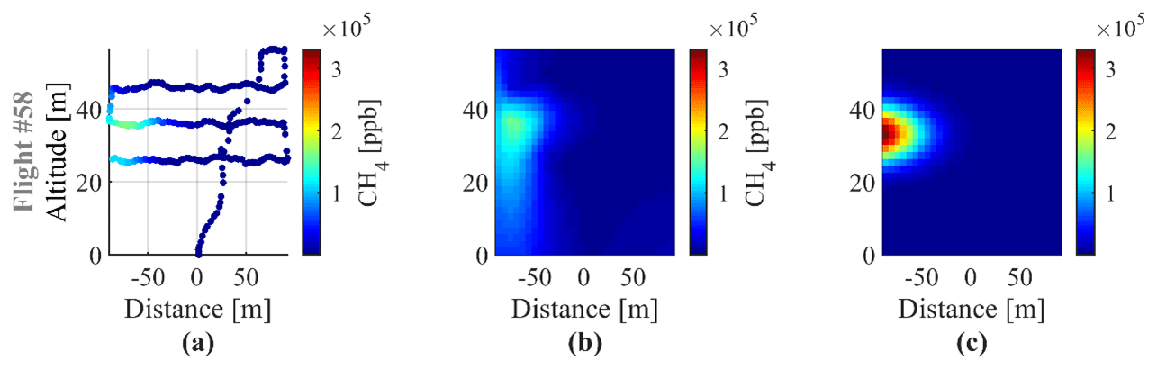
Figure 2(a) A sampled downwind CH4 mole fraction profile, (b) a kriged extrapolated 2D plane of CH4 mole fractions for the MB approach, and (c) an estimated 2D CH4 mole fraction plane using the parameters retrieved from the IG approach.
2.2 UAV-based active AirCore system
The active AirCore system was introduced in Andersen et al. (2018) and further refined in Andersen et al. (2021a). The active AirCore system is an air sampling tool that collects air along the trajectory of a UAV flight by pulling air through a long coiled stainless-steel tube. The pump is a small KNF020L micropump, which provides a vacuum downstream of a 45 µm pinhole orifice in order to create conditions for critical flow. Thus, the sampling flow rate of the AirCore only depends on the upstream pressure (ambient pressure), which is measured through the data logger, along with ambient temperature, ambient relative humidity, temperature within the carbon fiber box housing, and GPS coordinates. The inlet of the AirCore system was positioned to the side of the carbon fiber box that is beneath the propellers. Therefore, the air sampled into the AirCore is effectively from above the propellers, within less than 0.5 m above the propellers (Lampert et al., 2020). As the UAV is moving forward at a steady speed of 1–2 m s−1 most of time, the collected air samples will not be disturbed. This study used three different active AirCore systems, all of which have 0.32 cm ( in.) tubing. The lengths of the AirCore were 48.2, 46.9, and 48.5 m, with estimated volumes of 323, 315, and 325 cc, respectively. The UAV that the active AirCore system is attached to is a DJI Inspire Pro 1. Once an air sample has been obtained, the air is analyzed by a cavity ring-down spectrometer (CRDS, model no. G2401 m, Picarro Inc.) for CO2, CH4, and CO mole fractions. The CRDS used a high-CH4 analysis mode due to the large range of observed CH4 mole fractions (up to 200 ppm). A two-point calibration was used using a known WMO-scale gas mixture around ambient CH4 mole fractions (WMO X2007, X2004A, and X2014A scales for CO2, CH4, and CO, respectively) and a certified mole-fraction gas mixture from the Dutch National Metrology Institute (VSL) containing a high mole fraction of CH4 (301.1 ppm).
The AirCore samples were collected at the outlet of the Picarro, downstream of the pump, and were stored in Tedlar bags for further analysis of isotopic signatures of δ13C-CH4 and δ2H-CH4 at a later time in the laboratory using a continuous-flow isotope ratio mass spectrometer system. More details about the analytical system and the calibration are provided in Brass and Röckmann (2010), Röckmann et al. (2016), and Menoud et al. (2021). Out of the 59 flights performed during this study, the air samples from 34 flights were stored in Tedlar bags for further analysis of isotopic composition. Shafts Borynia VI, Pniowek IV, and Pniowek V had 2 separate days where isotopic compositions were measured, while Brzeszcze IX and Zofiowka IV had 1 d. Each day collected between four and five samples, which were used to determine the isotopic signature using a keeling plot.
AirCore concentration peaks are dampened due to molecular and Taylor diffusions in the sampling tube but mostly due to mixing of air samples in the cavity of the analyzer (Andersen et al., 2018). Deconvolving the measured signal to obtain the unaffected concentration peaks is possible, as is done in Andersen et al. (2021a). However, we have found that the moving averages of the original data using an averaging kernel of 33–34 s can match the convoluted signal well. Therefore, the simulated data from the Gaussian model is smoothed with such an averaging kernel before comparing with the AirCore observations. This was thus performed for all flights during the processing of the data.
2.3 Meteorological data
During the first four flights of the campaign, meteorological parameters (ambient temperature, pressure, relative humidity, wind speed, and wind direction) were measured using a radiosonde (Sparv Embedded AB, Sweden, model S1H2-R) identical to the one used in Andersen et al. (2021a). The radiosonde was tethered through a fishing pole for easier retrieval and reuse but was lost during the fourth flight due to getting too close to power lines. Four flights had radiosonde profiles to estimate the wind speeds and directions. The data for flight nos. 5 to 33 were obtained from a nearby meteorological station operated by the Polish meteorological office (IMGW). This was the Katowice Synoptic meteorological station, located at coordinates 50.240556∘ N, 19.032778∘ E. The use of this meteorological data, located a few tens of kilometers away from the measurement sites, may add significant uncertainty to the wind speed and direction for those flights, which was not quantified. For the second half of the campaign, from flight nos. 34 to 59, a mobile on-site meteorological station was used. The surface wind speed and wind direction were measured using a Campbell CSAT3 3-D Sonic Anemometer at about 1.5 m above ground. The mean differences in wind speed and wind direction between the Katowice Synoptic meteorological station and the mobile meteorological stations for flight no. 34 and onward were 1.7 ± 0.7 m s−1 and 38.8 ± 29.6∘, respectively. In this study, due to the lack of quantification of the additional uncertainty caused by the different meteorological data sources, we ignore their effects.
2.4 Emission determination
The emitted CH4 emanating from the ventilation shafts is quantified using the methodology derived in Andersen et al. (2021a). At each ventilation shaft, CH4 is vented to the atmosphere through one or more diffusers. Given the distance of 100–300 m between the UAV measurements and the ventilation shaft, the emission source can be regarded as a point source. The gridded plane is then used to quantify the emitted emission by applying an IG approach and a MB approach. The Gaussian model is given as follows:
where C′ is the dry mole fraction at a given position x, y, and z, which are the projected positional coordinates downwind of the plume, across the plume horizontally, and across the plume vertically (the units of are given in mol mol−1; the units of x, y, and z are given in m; the emission rate Q is given in kg s−1; the wind speed u is given in m s−1; and the stack height h is given in m). The parameters σy and σz describe the dispersion of the pollutants in the horizontal and vertical direction, respectively (in units of m). V is the dry molar volume (in m3 mol−1), and is the molar mass of CH4, 0.016 kg mol−1.
For the MB approach, the gridded flight pattern is extrapolated into a full 2D plane using a kriging method, to which the MB equation is applied. Figure 2 shows a measured UAV-based active AirCore profile of CH4 mole fractions, along with the 2D extrapolated kriged CH4 plane, and the IG's estimate plane of CH4 mole fractions. The MB equation is given as follows:
where Q is the output of the emission rate (in kg s−1); v is the wind speed (in m s−1) and assumed to be constant throughout the duration of the flights; ki is the number of horizontal grid boxes in the kriged plane; kj is the number of vertical grid boxes in the kriged plane; is the molecular mass of CH4 (in kg mol−1), Ci,j is the CH4 mole fraction in grid box i,j (in mol mol−1); ΔX is the area of each grid box (in m2); R is the universal gas constant (8.3145 ); T is the temperature (in K); and Pi,j is the pressure at each grid box (in Pa).
The minimum concentration of the entire flights was used as background, which was subtracted from the measured concentrations before calculation of the emissions for both the MB and the IG approach. The minimum concentration is not the same as a typical choice of, e.g., 10th percentile (Vinković et al., 2022); however, the difference of the two values is relatively small compared to the large CH4 enhancements and thus causes negligible difference in the calculated CH4 emissions.
The AirCore flight data (Y) presented in Fig. 2a is compared with the plume simulations of the Gaussian dispersion model. A best fit for Eq. (1) to the data can be found for these five parameters by minimizing the cost function using a standard square error (SSE) approach. The five parameters include the dispersion parameters in the horizontal and the vertical direction (σy and σz), the emission rate (Q), and the coordinates of the center of the plume in the curtain (height H and distance D). A group of random starting points for the five parameters between their lower and upper boundaries are set for the optimizer each time, and the optimization is run 1000 times to ensure that it is not only a local minimum that is found (Andersen et al., 2021a). In this way, we obtain a series of optimized values for each of the four parameters as the final results, and the five unknown parameters are optimized simultaneously.
A detailed description of the uncertainty analysis for both the IG and the MB methods has been presented in Andersen et al. (2021a). Here, we only give a brief description. The uncertainty of the IG method is calculated as the standard deviation of a series of optimized emission rates generated by a large number of optimization runs (N=1000). The uncertainty of the MB method is mainly determined by the uncertainty and the variability of wind speed and wind direction measurements.
2.5 Inventory emissions
The E-PRTR inventory gives the annual emission estimate for each coal mine in the Silesia region. An internal CoMet inventory, which is based on reported 2018 E-PRTR inventories (Gałkowski et al., 2021), lists 59 facilities related to coal mining operations in the USCB and divides the annual coal mine inventory by geo-localized (via Google Earth) active ventilation shafts for each coal mine. For the comparison used in this study, the active ventilation shafts are assumed to be the same as the ones stated in the internal CoMet inventory, but the E-PRTR values that are being divided equally among active shafts have been updated to the reported E-PRTR 2018 inventories. Pniowek, with a reported emission rate of 54.7 kt CH4 yr−1 and three active shafts, thus yields an average emission rate of 18.2 kt CH4 yr−1 for ventilation shafts Pniowek III, IV, and V. The inventory value for Borynia VI is 6.4 kt CH4 yr−1, for Zofiowka IV it is 13.9 kt CH4 yr−1, and for Brzeszcze IX it is 13 kt CH4 yr−1.
A second set of inventory data for May–June 2018 is also used for comparison during this study. These are hourly data calculated from raw CH4 concentration measurements and air flow rate measurements obtained within each specific ventilation shaft. Figure 3 shows a schematic design of a ventilation shaft. The concentration of CH4 is measured with an EMAG-Serwis-type DCH (EMAG Service: https://emagserwis.pl/metanomierze/, last access: 28 April 2023) methane sensor placed 10–15 m down into the exhaust shaft. This sensor has a measurement range of 0 %–100 % with a measurement error of 5 % of the reading value. The air flow rate is measured using a Prandtl's tube located between the main valve and the fan. According to Swolkień (2020), the relative uncertainty for the air flow rate is 10 %. According to the statements of ventilation engineers, the measured air flow includes about 5 % ambient air from the ventilation shaft closure, and we have taken that into account during the calculation of the hourly emission rates, i.e., CH4 concentrations multiplied by 95 % of the measured air flow rates.
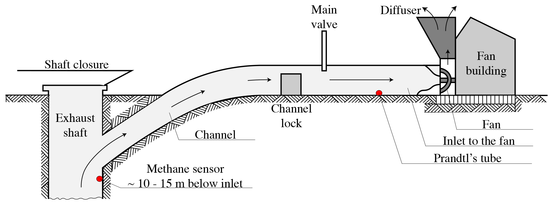
Figure 3Figure from Swolkień (2020, their Fig. 5) showing a coal mine ventilation shaft scheme. Their figure has been re-illustrated with updated graphics and readability for this paper. The original figure was published under a Creative Commons Attribution 4.0 International License, http://creativecommons.org/licenses/by/4.0/ (last access: 30 August 2021).
The conversion into CH4 emissions rate is done as follows:
where P is the atmospheric pressure (in Pa), R is the universal gas constant (in ), T is the ambient temperature (in K), Vflow is the volumetric flow rate of CH4 (in m3 s−1), given by the air flow rate multiplied by the CH4 concentration. Lastly, ρ is the molar density of CH4 (in g mol−1) (16.043 g mol−1). A temperature of 20 ∘C and a pressure of 101 325 Pa were used for the calculation.
2.6 Upscaling
As mentioned in Sect. 2.3, more than 70 facilities related to coal mining operations are located in the USCB. According to the internal CoMet inventory, 59 are active ventilation shafts. After obtaining CO2 and CH4 emissions from 5 of the 59 shafts in the USCB, three distinct approaches are used to obtain an estimate of the regional emission rate.The first method uses the linear correlation of shaft-averaged emissions between our UAV-quantified and high-frequency (hourly) reported emissions to scale the annual E-PRTR emissions. To avoid the large influence of the intercept, the linear curve has been forced through zero, making the slope the only factor to scale the emissions. The second approach uses the mean quantified shaft emissions, multiplied by the number of ventilation shafts in the region. The third approach scales the mean hourly inventory emission rate to derive the mean quantified emission rate based on the linear correlation of shaft-averaged emissions between our UAV quantified and high-frequency (hourly) reported emissions, which is then multiplied by the number of active ventilation shafts in the region. The equations are shown below:
where QE-PRTR-regional is the annual E-PRTR emission rate, is the mean quantified shaft emission rate, is the mean hourly inventory emission rate, k2 and b are the slope and the intercept of the linear fit of shaft-averaged emissions between our UAV quantified and high-frequency (hourly) reported emissions, k1 is the slope of the linear fit that is forced through zero, and n is the number of active ventilation shafts in the region.
3.1 Isotopic signature
Figure 4 shows the sampled isotopic signatures of δ13C-CH4 and δ2H-CH4 from the flights during the study, separated into different shafts and different days. For the five sampled ventilation shafts, the δ13C-CH4 values ranged between −53.4 ‰ and −41.3 ‰, while the δ2H-CH4 values ranged between −175.0 ‰ and −151.2 ‰. According to Sherwood et al. (2021), isotopic signature values from coal mining vary from country to country, and the source signature in Poland was found to be −48 ‰ ± 15 (±1σ) ‰ for δ13C-CH4 and −194 ± 37 for δ2H-CH4. Source signatures found during the same measurement campaign, CoMet 1.0, by other groups indicate that the source signatures for δ13C-CH4 and δ2H-CH4 in the Upper Silesian Coal Basin range between −59.4 ‰ to −41.0 ‰ and −218 ‰ to −142 ‰, respectively (Stanisavljevic, 2021). Overall, the addition of δ13C-CH4 and δ2H-CH4 measurements and the good agreement between the found source signatures with those of other groups during the same campaign indicate that we have clearly sampled the coal mine ventilation shafts using the UAV-based active AirCore system. Based on what is shown in Fig. 4 it is unlikely that other regional CH4 sources (such as biomass burning, landfills, and ruminants) have influenced the active AirCore measurements.
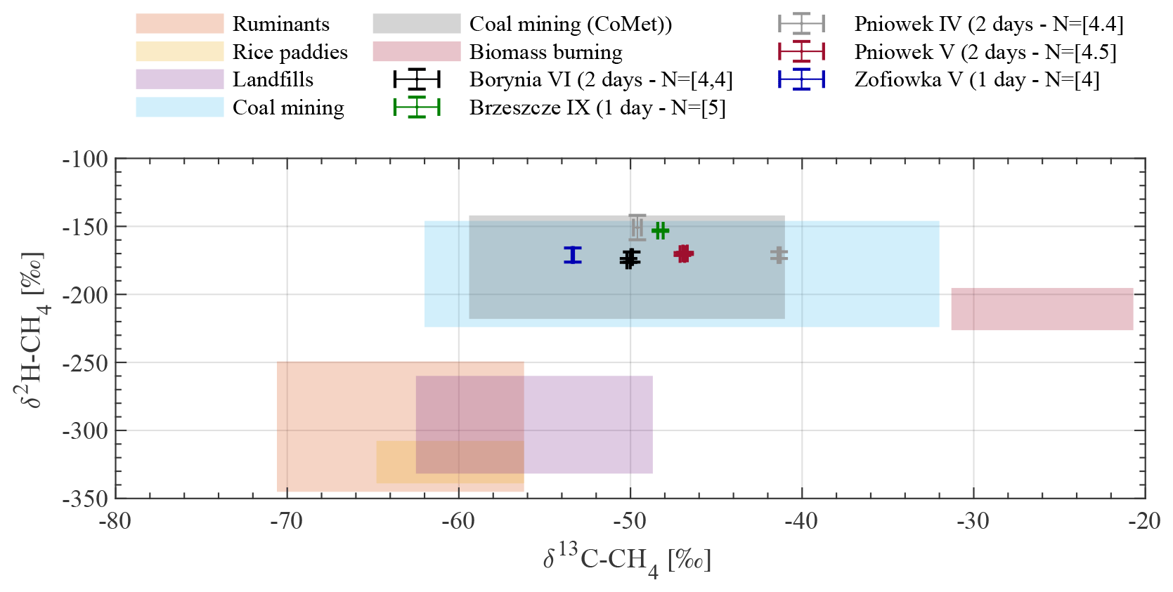
Figure 4Scatterplot indicating the isotopic signature for each measured ventilation shaft. The shaded areas indicate typical δ13C-CH4 and δ2H-CH4 values for different CH4 sources and are given with a 1σ uncertainty. The values and uncertainties for coal mining are determined from measurements in Poland, and for other sources from the whole world (Sherwood et al., 2021; Lan et al., 2021). The gray-shaded area indicates the isotopic signatures found from other groups during the CoMet 1.0 campaign and represents the calculated weighted average for the coal in the USCB (Stanisavljevic, 2021; Menoud et al., 2020).
3.2 Quantified CH4 emissions
Figures 5 and 6 show the estimated CH4 emission rates from individual ventilation shafts, for each day, along with the hourly inventory presented in the next section. Averages range between 2.7 ± 2.0 and 15.0 ± 2.3 kt yr−1 for the IG approach, and between 0.8 ± 1.0 and 14.4 ± 3.7 kt yr−1 for the MB approach. Large variations are seen on a day-to-day basis for the same coal mine ventilation shafts. The IG approach and MB approach have a mean difference of 2.5 kt yr−1, with a maximum difference of 8.9 kt yr−1 on 31 May. This is likely due to the majority of the plume being located outside of the gridded curtain, which causes the IG to move the center line of the plume off the grid to obtain the best fit between model and data, while the MB is constrained to only include what is included in the kriged plane. The same is seen in the first flight on 25 May for Pniowek IV (see Fig. 6), where the majority of the IG plume is located outside the measured grid. Note that both the IG and MB approaches have been applied to all flights that fulfilled the criteria. The missing quantifications from the IG method for some flights are entirely due to failures of the optimization. For example, observed concentrations on adjacent flight tracks are inconsistent due to plume meandering in one flight, as is shown in Fig. A1 (no. 9), making it impossible to find an optimized set of parameters within their reasonable boundaries. The uncertainty in the emissions quantified by UAV-based AirCore measurements is linked to the stability of the wind, as discussed in Andersen et al. (2021a). The 10–12 min snapshots are not instantaneously sampled, and an unstable wind may cause the emission plume to meander across the plane.
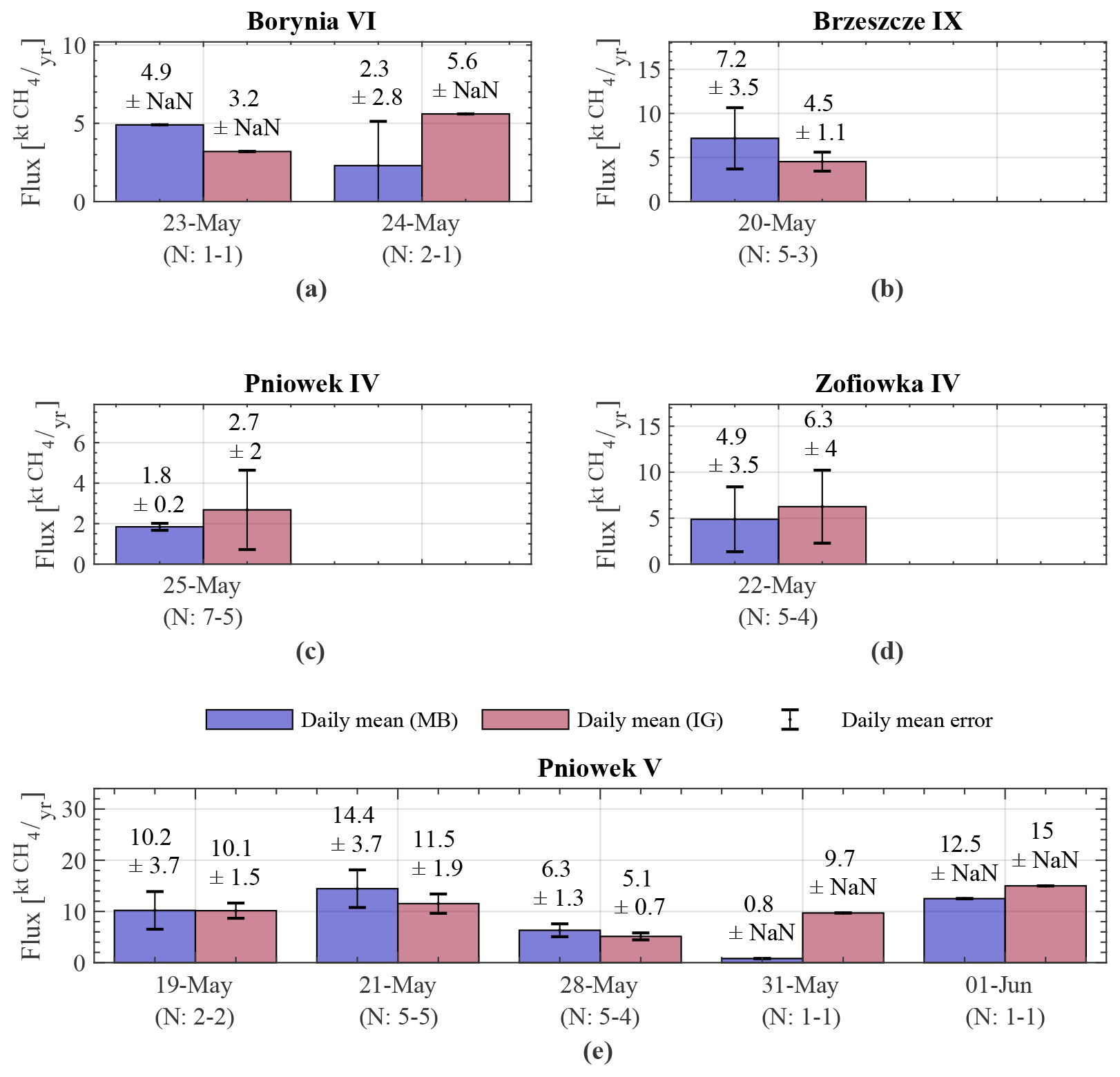
Figure 5CH4 emission estimates for each ventilation shaft per measurement day. Light red shows the IG approach; light blue shows the MB approach. The bar height is the average of all flights during a specific day. The error bar indicates the standard deviation of the individual flights for that specific day, where the number of flights used for each bar is indicated with N. The two values for N refer to the MB approach and IG approach, respectively. The error is indicated as NaN when only one estimate is available.
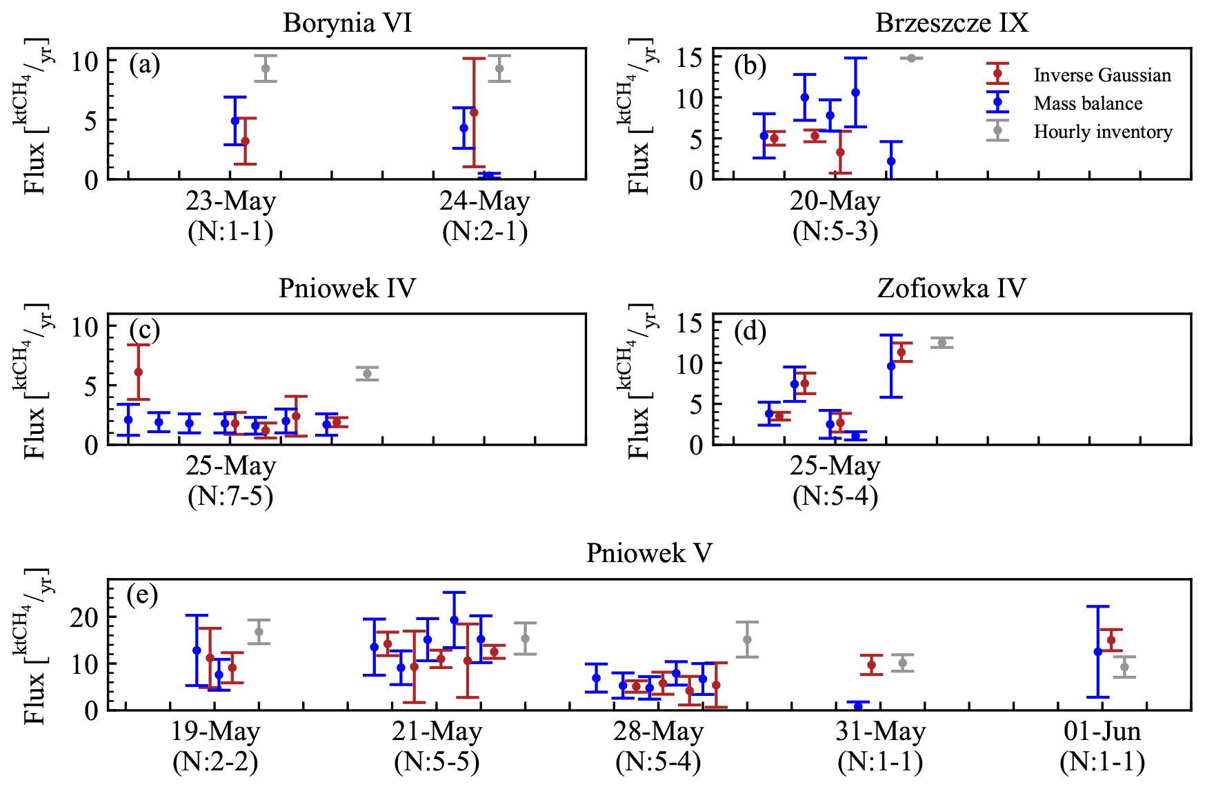
Figure 6The quantified CH4 emission for each flight divided into different ventilation shafts and separated by individual flight days with the hourly inventory. The emissions are also color differentiated by IG approach (red) or MB approach (blue). The number of quantifications on each day from the two methods is indicated in the parentheses.
3.3 Comparison with inventory
Figure 7 shows the hourly inventory emissions for each ventilation shaft. The inventory reported to the E-PRTR is based on these data. Note that inventory measurement for Borynia VI is missing for the period between 19 and 30 May (Fig. 7a). We did not receive any specific explanation for the missing data and assume this was due to a malfunctioning CH4 sensor inside the ventilation shaft. The listed inventory data for Borynia VI in Table C1 was therefore calculated with data from 30 May–2 June. The Borynia VI inventory may therefore not represent the actual inventory of the days of measurements. The same can be concluded for Brzeszcze IX (Fig. 7b), which only has one given measurement point. The variability in the emitted CH4 is clearly seen in the data from Pniowek IV, Pniowek V, and Zofiowka IV (Fig. 7c–e).
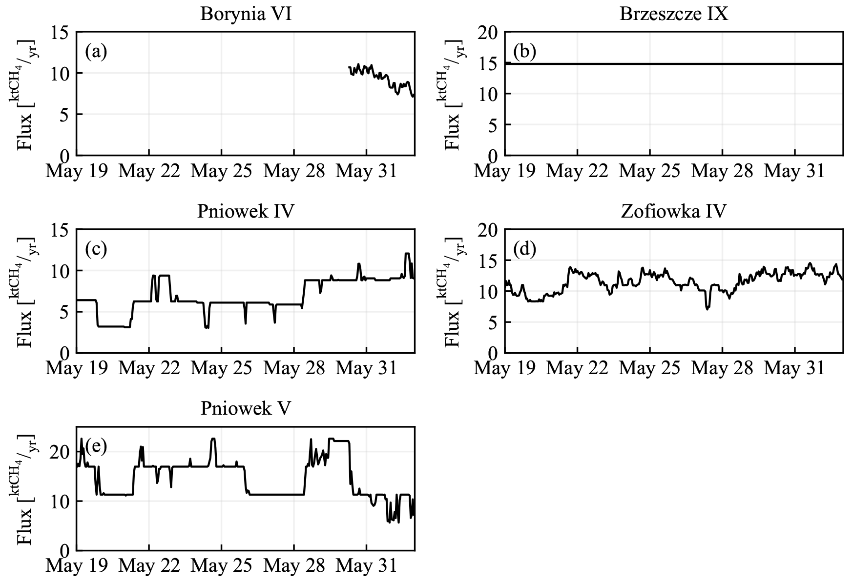
Figure 7Time series of hourly inventory emissions from CH4 concentration and air flow measurements in the shaft for each investigated coal mine ventilation shaft. Prior to 30 May, data in (a) are missing. In (b) only a constant value is available from 19 May–1 June.
In comparing the quantified CH4 emission rate on an individual flight basis with the annual emission rate reported to the E-PRTR, we found that the correlation is very low (R2<0.05). Figure 8a shows the correlation between the E-PRTR annual emissions that has been divided by the number of active ventilation shafts for a particular coal mine and the UAV-based active AirCore IG quantified CH4 emissions averaged by shaft emissions. Also, here the correlation is low (R2<0.08, N=5). When the total reported mine emissions for a specific mine from the E-PRTR inventory are divided equally by the number of active shafts, shaft-specific emission info is lost. The non-existent correlation indicates that the agreement between the snapshot flight quantified emissions with the E-PRTR inventory is poor.
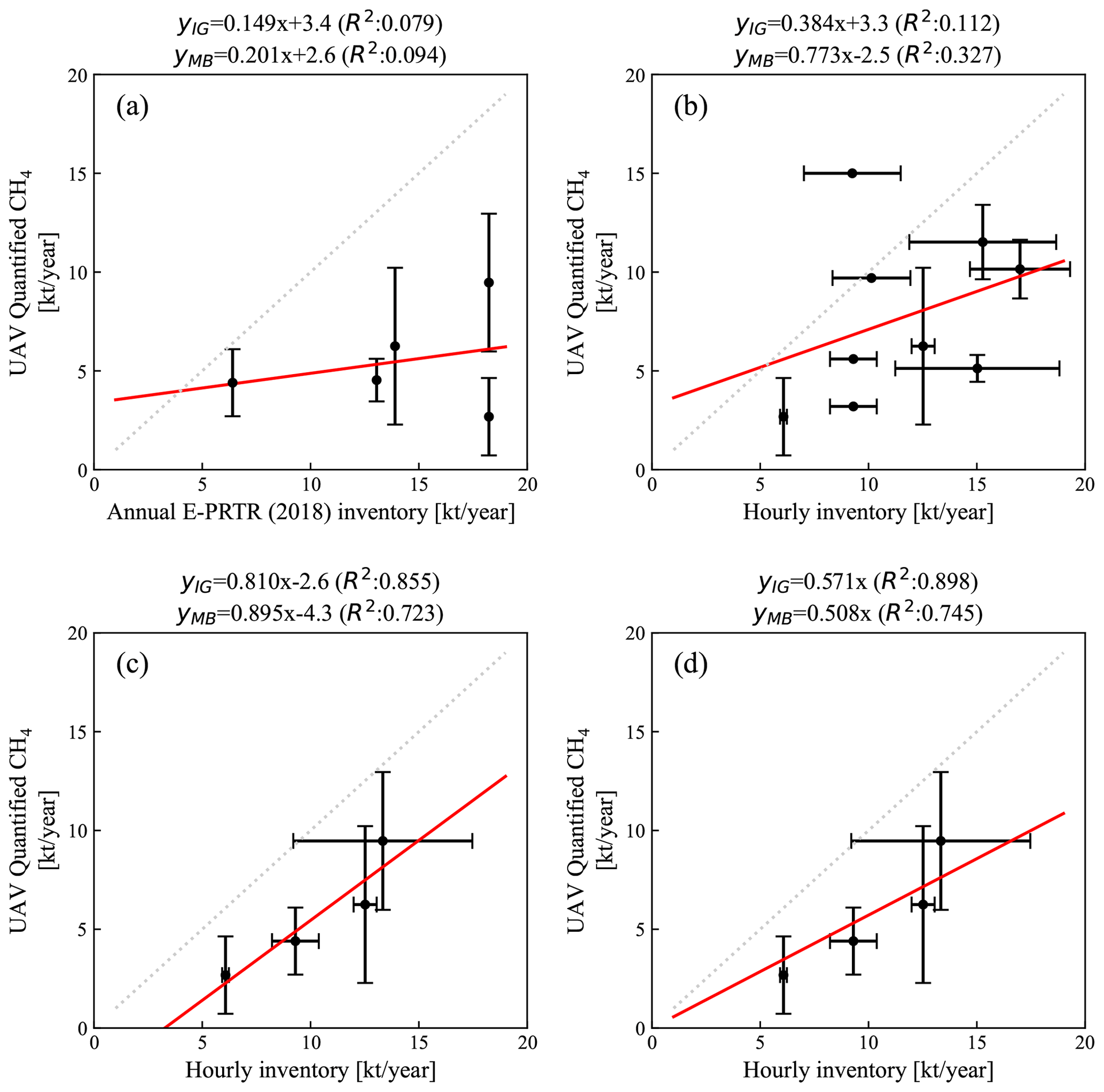
Figure 8Scatterplot of UAV-quantified shaft-averaged emissions over multiple days or individual days against annual or hourly inventory data. (a) Shaft-averaged quantified emissions over multiple days vs. annual coal mine emissions from the E-PRTR 2018 (Gałkowski et al., 2021) inventory. (b) Daily shaft-averaged quantified emissions vs. daily high frequency (hourly) shaft-averaged inventory. (c) Shaft-averaged quantified emissions over multiple days vs. shaft-averaged high frequency (hourly) inventory over the same days. Panel (d) is the same as (c) except that the fit has been forced through origin. The red lines indicate linear fits, and the parameters are shown in the title. All panels display only the data from the IG approach; however, the title lists the curve fit from the MB approach as well. The E-PRTR inventory has been divided by the number of active ventilation shafts, and the number of active shafts is taken from the internal CoMet inventory, which had emission profiles based on 2018.
The hourly inventory data shown in Fig. 8b are therefore required for a direct comparison with the quantified emissions. Comparing these data on a daily averaged basis with daily averaged flight data sees a slight improvement in the obtained correlation (R2=0.11, N=9), although the correlation is still weak. Due to the lack of hourly data for Brzeszcze IX, it has been omitted for the comparison. There can still be large variations on an hourly basis, and thus a direct comparison between the hourly inventory over a day with snapshot flight profiles during the same day may not always align. Therefore, we have averaged the days together and compare shaft-specific averaged hourly data with shaft-specific averaged UAV quantified emissions from the same days. This is shown in Fig. 8c, which obtains a stronger correlation than the two previous comparisons, with an R2=0.86 (N=4). The quantified emissions are roughly 50 % lower than those of the hourly inventory; however, this is not significant when considering the large standard deviation of the measurements.
The much-improved correlation from comparing hourly inventory data from individual shafts as opposed to a total mine emission divided equally over active shafts (i.e., based on the E-PRTR 2018 inventory) indicates that translating shaft-quantified snapshot emissions to annual inventories is difficult. The hourly inventory data are not always available, but our evaluations indicate that they are required to make meaningful comparisons between quantified emissions and inventories. Due to the good correlation between the hourly inventory and the quantified emissions per shaft, we can use the hourly inventory data to scale up the quantified emissions. We use the slopes and the intercepts found in Fig. 8c to scale up our quantified emissions. This will be discussed in Sect. 4. For the MB approach (data not shown), the correlations are also much improved when hourly inventory data are used for comparison, although the R2 values are slightly lower than those for the IG approach.
Figure 9 shows the boxplot comparison between estimated emissions from both the IG approach and the MB approach against the hourly inventory for each ventilation shaft. The inventory data include data for the same days as the flights except for those of Borynia VI and Brzeszcze XI. As previously mentioned, Brzeszcze XI contains only an annual estimate, while for Borynia VI inventory data are missing for the specific days when this shaft was sampled. Pniowek V, the shaft with the most overflights (N=13 for the IG and N=14 for the MB approach over 5 different days), has largely overlapping distributions with the hourly inventory data, although these lean towards the lower end of the hourly inventory distribution. Pniowek IV and Zofiowka IV have N=5 / N=4 for the IG and N=7 / N=5 for the MB, respectively. Zofiowka IV has overlapping distributions with the hourly inventory, but the quantified emissions largely span the lower hourly inventory distribution. This is seen with all other shafts as well. Pniowek IV has only a small overlap with the hourly inventory distribution for the IG approach. Brzeszcze IX is difficult to compare due to the lack of hourly inventory data, and the only hour inventory data match the upper end of the IG estimates. Finally, Borynia VI has the fewest flights, with N=2 for the IG and N=3 for the MB approach over 2 different days. There is no overlap between the distributions. Borynia VI and Brzeszcze IX are difficult to compare due to the lack of direct hourly inventory data around the days of flying.
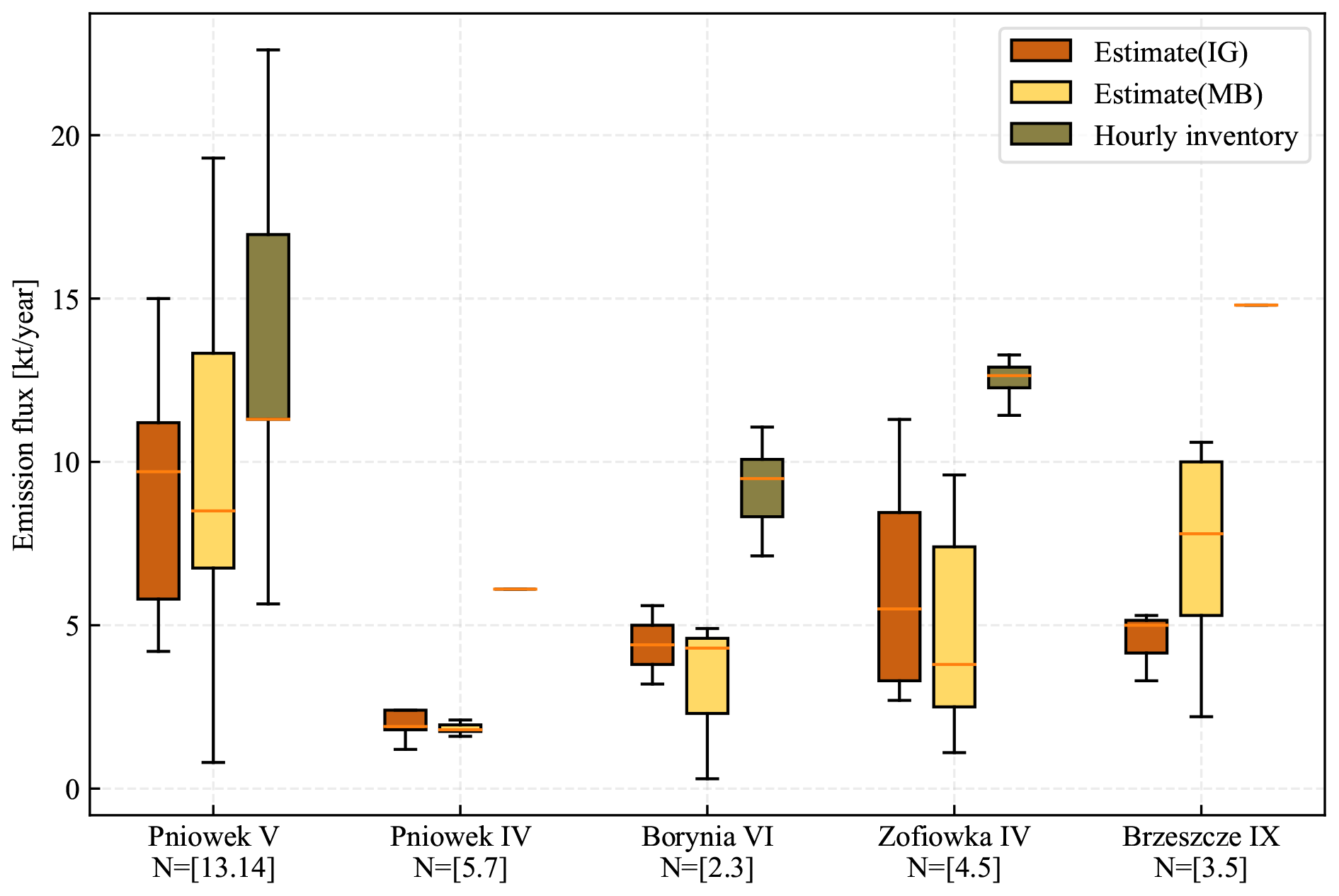
Figure 9Boxplot comparison of estimated emission vs. hourly inventory data. The hourly inventory data have been calculated from shaft emission data from the mining companies, using CH4 concentration and flow rate measurements.
Thus, the measured distributions for Pniowek V, Pniowek IV, and Zofiowka IV overlap with the hourly inventory distributions, with a minimum of N≥5 flights. The largest overlap is as mentioned found in Pniowek V, containing several days of sampling and N≥13. These distribution comparisons suggest that although single flight estimates may not be correlated well with the hourly inventory, the averaged estimates of multiple flights show a strong correlation with those of the inventory, which suggests that multiple flights are required to obtain a good estimate. Note that for all shafts, the UAV estimated emission distribution is located on the lower end of the inventory distribution. This could be due to a lack of statistics in the number of quantifications or the possible biases of the measured hourly inventory. As for the uncertainties for the two estimate methods, the mass balance approach is limited by the measurement time and range, and the inverse Gaussian approach suffers from non-Gaussian plume behavior due to local turbulence and lack of temporal average, which are quite challenging, and further study is needed.
3.4 Carbon dioxide emission
Similar to the coal mining shaft sampled in Andersen et al. (2021a), a strong correlation is found between the emitted CO2 and CH4. The way of obtaining the emitted CO2 using the correlation between CO2 and CH4 mole fractions, the CH4 emissions, and the molar mass constants of CO2 and CH4 is given as follows:
where is the quantified CH4 emission, the slope is the slope of the linear fit between CO2 and CH4 (), and and are the molar masses of CO2 and CH4, respectively. There were some flights that had no or low correlation and were thus omitted from the CO2 emission calculation (see Figs. B1–B4). These were flights with R2<0.5. Of the 34 flights that fulfilled the criteria list, the number of flights above an R2 value of 0.5 was 25, with an average R2 of 0.8. The average slope was 4.6 ± 2.9 ppm CH4 per ppm CO2. We have used the linear correlation between enhanced CH4 and CO2 to calculate the CO2 emissions instead of directly using the CO2 data for two reasons: (1) the CO2 signal is relatively small compared to its variabilities, which makes it difficult to find a robust background signal, and (2) we aim to quantify the CO2 emissions from the shaft only.
Figure 10 shows the calculated CO2 emission on a daily averaged basis for each coal mine ventilation shaft. Expectedly, the CO2 estimates also show strong variations on a day-to-day basis, as is the case for the CH4 estimates. The mean difference between the IG and the MB approach is 1.5 kt yr−1. The average CO2 emission rate over all shafts calculated using the IG approach is 4.4 ± 2.2 kt yr−1, with a minimum of 0.8 ± NaN kt yr−1 and maximum of 7.2 ± 4.1 kt yr−1. For the MB approach, the average CO2 emission rate is 3.8 ± 2.3 kt yr−1, with a minimum of 0.5 ± NaN kt yr−1 and maximum of 7.5 ± 1.8 kt yr−1.
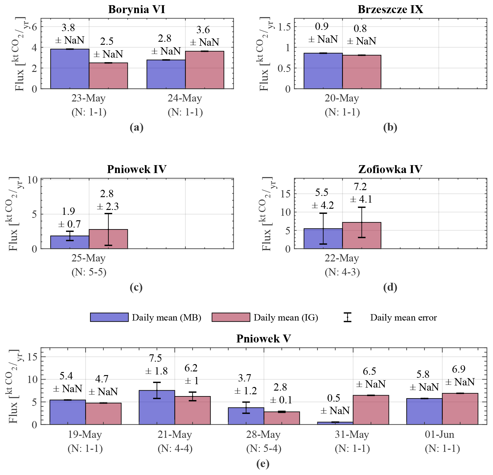
Figure 10This figure shows CO2 emission bar plots for each ventilation shaft divided into separate days. Emission quantifications for both the IG approach (light red) and MB approach (light blue) are shown. The bar height is the mean of all flights during a specific day. The error bar is indicated as NaN when only one estimate is available.
3.5 Upscaling to regional estimates
As shown in Table C1, the mean quantified CH4 emission of the five sampled coal mine ventilation shafts is 5.5 ± 2.6 kt CH4 yr−1 for the IG approach and 5.4 ± 3.2 kt CH4 yr−1 for the MB approach. For CO2, the mean emission is 4.2 ± 2.2 kt CO2 yr−1 for the IG approach and 3.8 ± 2.3 kt CO2 yr−1 for the MB approach. As many as 59 active ventilation shafts are located across the entire USCB. According to the 2018 E-PRTR inventory, the regional CH4 emissions add up to 447.9 kt CH4 yr−1, while the regional CO2 emissions are stated to be 35.3 [Mt CO2 yr−1].
Three distinct approaches have been used to obtain an estimate of the regional emission rate. The first method uses the linear correlation of shaft-averaged emissions between our UAV quantified and high frequency (hourly) reported emissions shown in Fig. 8d to scale the annual E-PRTR emissions. Here we assume that the correlation between the shaft-averaged hourly inventory and UAV-quantified emissions are representative for the whole basin and that the very low correlation between the shaft-averaged E-PRTR inventory and UAV-quantified emissions is mainly due to large errors introduced to the E-PRTR inventory for individual shafts by dividing the inventory for individual coal mines by the number of active shafts. To avoid the large influence of the intercept, the linear curve has been forced through zero, making the slope the only factor to scale the emissions. For the IG approach, the slope is 0.571, which multiplied with the 447.9 kt CH4 yr−1 inventory results in 255.8 kt CH4 yr−1. For the mass balance, with a slope of 0.508, the resulting emissions are 227.5 kt CH4 yr−1. These results are shown in Fig. 11a as yellow bars.
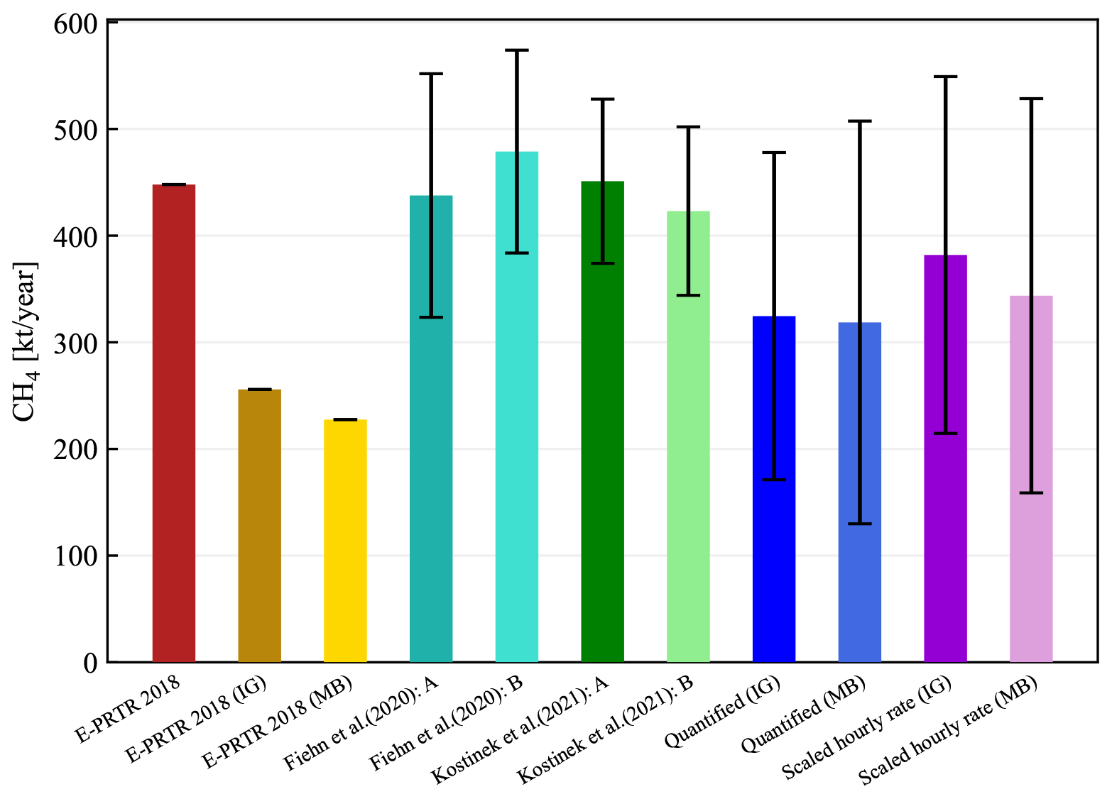
Figure 11A comparison of regional inventory emissions for CH4. The first bar (red) represents the E-PRTR inventory. The second and third bars represent the E-PRTR inventory scaled by the different linear fits of IG and MB approaches. Bars four and five (teal) represent the estimated regional emissions from Fiehn et al. (2020) from their two flights. Bars six and seven (green) represent the estimated regional emissions from the two flights of Kostinek et al. (2021). Bars number eight (blue) and nine (light blue) represent the regional emission using the quantified IG and MB estimates, respectively. The last two bars, 10 (purple) and 11 (light purple), represent the scaled regional emission using the IG approach and the MB approach, respectively.
The second approach uses the mean quantified shaft emissions of 5.5 ± 2.6 kt CH4 yr−1 for the IG approach and 5.4 ± 3.2 kt CH4 yr−1 for the MB approach, multiplied by the number of ventilation shafts in the region. This amounts to a regional emission of 324.5 ± 153.4 kt CH4 yr−1 for the IG approach and 318.6 ± 188.8 kt CH4 yr−1 for the MB approach. These emission estimates compare well with the ones from the previous approach but are lower than the emissions estimated by Fiehn et al. (2020) and Kostinek et al. (2021). These are shown in Fig. 11a as blue bars. We acknowledge that potentially large biases may have been introduced to the upscaling as the number of quantified shafts (5) is small compared to the total number of shafts (59).
The third approach uses the line from Fig. 8c to scale the mean hourly emission rate, calculated from hourly inventory data, to derive the mean quantified emission rate, which is then multiplied by the number of active ventilation shafts in the region. Here, both the slope and intercept are used for the scaling. The mean hourly inventory emission rate is 11.2 ± 3.5 kt CH4 yr−1. The line using the IG approach has a slope of 0.81 and an intercept of −2.6, resulting in a derived mean quantified emission rate of 6.5 ± 2.8 kt CH4 yr−1. For the mass balance, a slope of 0.895 and an intercept of −4.3 results in a derived mean quantified emission rate of 5.7 ± 3.1 kt CH4 yr−1. Multiplying these numbers with the number of active ventilation shafts results in regional emission rates of 383.1 ± 165.8 kt CH4 yr−1 for the IG approach and 339.0 ± 183.4 kt CH4 yr−1 for the MB approach. The regional estimates for the IG approach and MB approach resulting from the third upscaling approach are shown in Fig. 11 as purple bars.
Comparing the IG-derived regional emission with both the annual E-PRTR inventory and the regional estimates from Fiehn et al. (2020), the results are close to one another and are not statistically different when their uncertainties are considered, although the uncertainties are as large as 20 %–43 %. Fiehn et al. (2020) estimated the regional emissions over two separate flights during the same CoMet campaign to be 437.6 ± 114.2 and 478.8 ± 95.1 kt CH4 yr−1, similar to the 447.9 kt CH4 yr−1 E-PRTR inventory. Kostinek et al. (2021) also estimated the regional emissions over two separate flights and found emissions rates of 451 ± 77 and 423 ± 79 kt CH4 yr−1. Our estimated emissions appear to be lower. Since we have only quantified 5 individual shafts out of 59 active shafts in the region, the small number of quantified shafts could be one of the main causes of the difference.
The upscaling process for CO2 cannot be explored by the same approaches as for CH4 since the linear fits from Fig. 8 are only valid for CH4. Therefore, only the second approach can be used, where the mean quantified CO2 emission will be multiplied by the number of active ventilation shafts in the region. According to Swolkien (2020), there are colocated CO2 emissions and CH4 emissions during the extraction of coal. However, CO2 emissions from coal mining activities are not included in the E-PRTR inventory. The mean CO2 emission is 4.2 ± 2.2 kt CO2 yr−1 for the IG approach and 3.8 ± 2.3 kt CO2 yr−1 for the mass balance, which yields a regional emission estimate of 0.25 ± 0.13 Mt CO2 yr−1 for the IG approach and 0.22 ± 0.14 Mt CO2 yr−1 for the MB approach. This is significantly less than the E-PRTR inventory of 35.3 Mt CO2 yr−1 and the estimated regional emissions rates from Fiehn et al. (2020) of 38.2 ± 22.7 and 35.3 ± 11.7 Mt CO2 yr−1. Comparatively, these estimates are ∼1 % or less of the listed E-PRTR inventory. According to the E-PRTR (2018) inventory, 98.2 % of emitted CH4 in the USCB originates from underground and related operations, 1.5 % comes from opencast mining and quarrying, and 0.3 % come from waste and waste water management. For CO2, the major contributors are thermal power stations and other combustion installations and production and processing of metals. These account for 78.9 % and 16.3 %, respectively. Residential heating accounts for 2.6 %, while other industrial manufacturing accounts for 2.2 %.
The upscaling method uses daily snapshots to estimate an annual emission by multiplying the annual average of the five sampled shafts by the number of ventilation shafts in the region. As shown in Sect. 3.3, each ventilation shaft can have significant variations in its daily emissions; thus, this adds uncertainty to the daily snapshots extrapolated to an annual emission. Ventilation shafts can have significantly different emission rates, thus grouping the five shafts together to obtain the average does not accurately represent the emission distribution in the whole region. This adds additional uncertainty to the upscaled regional emission. Despite this, we see a good agreement with the two flights from Fiehn et al. (2020), Kostinek et al. (2021), and the E-PRTR inventory for CH4 within the error bars (see Fig. 11a), especially using the third approach of deriving the quantified emissions from hourly inventory data and scaling this to a regional emission rate. This indicates that the upscaling of the ventilation shaft emissions estimated from the UAV-based active AirCore can be a useful tool for relatively cheap and easy-to-obtain regional emission estimates. Estimated regional CO2 emissions from these coal mines are vastly smaller than the suggested regional inventory and also the regional emissions found by Fiehn et al. (2020). The estimated regional CO2 emissions are ∼1 % of the regional inventory estimate and would be equivalent to the emissions of ∼130 000 and ∼120 000 automobiles (assuming 7 L or 18.9 kg CO2 per 100 km and an average of 10 000 km driving per year) for IG and MB estimates, respectively, confirming that the coal mine ventilation shafts are not a major source of CO2 in the USCB. This is also reflected in the E-PRTR inventory, which does not list coal mining as a CO2 source at all.
It is important to obtain independent estimates of the emission magnitudes from coal mining shafts and verify reported emission inventories to be able to reduce the overall emissions. Using the UAV-based active AirCore system, we have made atmospheric measurements of CH4 and CO2 mole fractions downwind of five different coal mine ventilation shafts in the USCB. We apply an IG approach and an MB approach to quantify the CH4 and CO2 point source emissions for the five sampled ventilation shafts and compare these estimates with reported inventory data. The estimated point sources are used to extrapolate a total USCB regional CH4 and CO2 estimate.
The CH4 emission estimates indicate that the coal mine ventilation shafts have highly variable emission rates. Over the five quantified shafts, the quantified emissions using the IG approach range between 1.2 and 15.0 kt CH4 yr−1, with a mean of 5.5 ± 2.6 kt CH4 yr−1. For the MB approach, the quantified emissions range between 0.3 and 19.3 kt CH4 yr−1, with a mean value of 5.4 ± 3.2 kt CH4 yr−1. This large variability is reflected in the hourly inventory data for the same coal mine ventilation shafts, and it is therefore clear that comparisons of the UAV-based active AirCore quantified emissions and annually averaged inventories show very low correlation (R2=0.08). Day-by-day comparisons of the quantified emissions with an hourly inventory during the same days yields a better correlation (R2=0.11), but the best correlation is found on shaft-by-shaft comparisons, obtaining an R2 of 0.86 for the IG approach and 0.72 for the MB approach. Distribution comparisons between the hourly inventory and the quantified emissions show that more flights are beneficial to accurately estimate the shaft emissions. Due to the large variability of the shaft emissions, single flights may sample at times of small or large emission. Correlation between CH4 and CO2 mole fractions is large for 25 out of 34 flights (average R2=0.8) and has an average slope value of 4.6 ppm CH4 per ppm CO2. Quantified CO2 emissions for the combined five ventilation shafts yield an average of 4.4 ± 2.2 kt CO2 yr−1 for the IG approach and 3.8 ± 2.3 kt CO2 yr−1 for the MB approach.
To obtain regional estimates, we use three upscaling approaches by scaling the E-PRTR annual inventory, the quantified shaft-averaged emission rate, and the shaft-averaged emission rate, which are derived from the hourly emission inventory. The first approach obtains emission rates of 256 kt CH4 yr−1 from the inverted Gaussian approach and 228 kt CH4 yr−1 from the MB approach, respectively, which compares well with the second approach of 325 ± 148 (Gaussian) and 318.6 ± 189 kt CH4 yr−1 (mass balance). These estimates are lower than the previous results from Fiehn et al. (2020), Kostinek et al. (2021), and the E-PRTR inventory of 448 kt CH4 yr−1. The third approach results in regional emission estimates of 383 ± 165.8 (Gaussian) and 339 ± 183 kt CH4 yr−1 (mass balance), providing a good comparison with both the E-PRTR inventory and previous results from Fiehn et al. (2020) and Kostinek et al. (2021). The differences are not significant when the relatively large uncertainties are considered. Upscaled regional emissions for CO2 amount to 0.2–0.3 Mt CO2 yr−1 for both quantification approaches, which is ∼1 % of the reported inventory and regional CO2 estimates from Fiehn et al. (2020), confirming that the coal mine ventilation shafts are a minor contributor to the regional CO2 emissions.
The uncertainty in the emissions quantified by UAV-based AirCore measurements is linked to the stability of the wind, as discussed in Andersen et al. (2021a). The 10–12 min snapshots are not instantaneously sampled, and an unstable wind may cause the emission plume to meander across the plane. Although a single flight may not accurately represent the ventilation shaft emissions, this study shows that with multiple flight quantifications for a single shaft, a good estimate of the shaft's emission rate can be made. Unfortunately, we do not have specific information on the impact of seasonal changes on emissions in this region, and we are aware that short-term flights over the span of 2 weeks are used to estimate an annual average, where emission rates may vary week-to-week, and thus it is necessary to consider the effect of time on emission rates in 1 year. The E-PRTR shaft-scale estimates assume that all shafts of a single coal mine emit an equal amount, which clearly is not true. A more accurate upscaling model taking into account the individual emission size of different shafts would help improve this estimate.
The use of UAV-based active AirCore measurements in combination with the IG approach and the MB approach has been demonstrated to be able to quantify the emissions from individual ventilation shafts, which can then be used to estimate regional emissions of both CH4 and CO2. However, the uncertainty of individual flight quantification may be large due to variable wind conditions under complexed turbulent schemes. Also, the in situ plume sampled by the AirCore does not necessarily follow the assumed Gaussian dispersion, as the averaging time is not sufficiently long, i.e., less than 30 min, which inevitably increases the uncertainty of the estimates by the IG method. To this end, optimization schemes that do not rely on the simple assumption of a Gaussian dispersion may be valuable (Shi et al., 2022). On the other hand, the complex dispersion of the plume can be simulated by 3D large-eddy simulation (LES), which can provide guidance to the design of the sampling strategy and help develop a suitable method to estimate the emission rates based on the in situ plume sampling (Ražnjević et al., 2022).
The uncertainty of the estimate of an individual shaft can be reduced by increasing the number of the quantification flights, although it is challenging to determine the exact number of needed flights to achieve a target uncertainty. Analysis of a large number of controlled tracer release experiments may provide an opportunity to directly address this issue, as has been performed for UAV measurements and many other different measurement platforms (Feitz et al., 2018; Bell et al., 2020; Morales et al., 2022).
Also, the uncertainty of the regional estimates can be reduced by increasing the number of quantified shafts. The limited number of quantified shafts makes our upscaling to the regional emission vulnerable. Nevertheless, the UAV system is flexible and versatile and opens up opportunities to quickly obtain regional estimates in regions that are otherwise hard to access. The UAV-based active AirCore system has thus been shown to be a valuable tool to estimate CH4 emissions on local to regional scales.
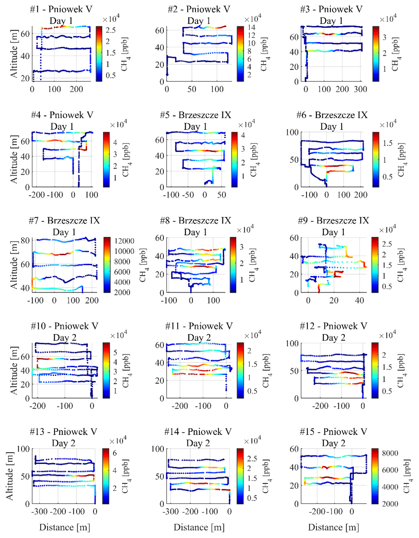
Figure A1The measured flight profiles for flight nos. 1 to15. Flight nos. 1, 4, and 13 are excluded according to the flight selection criteria.
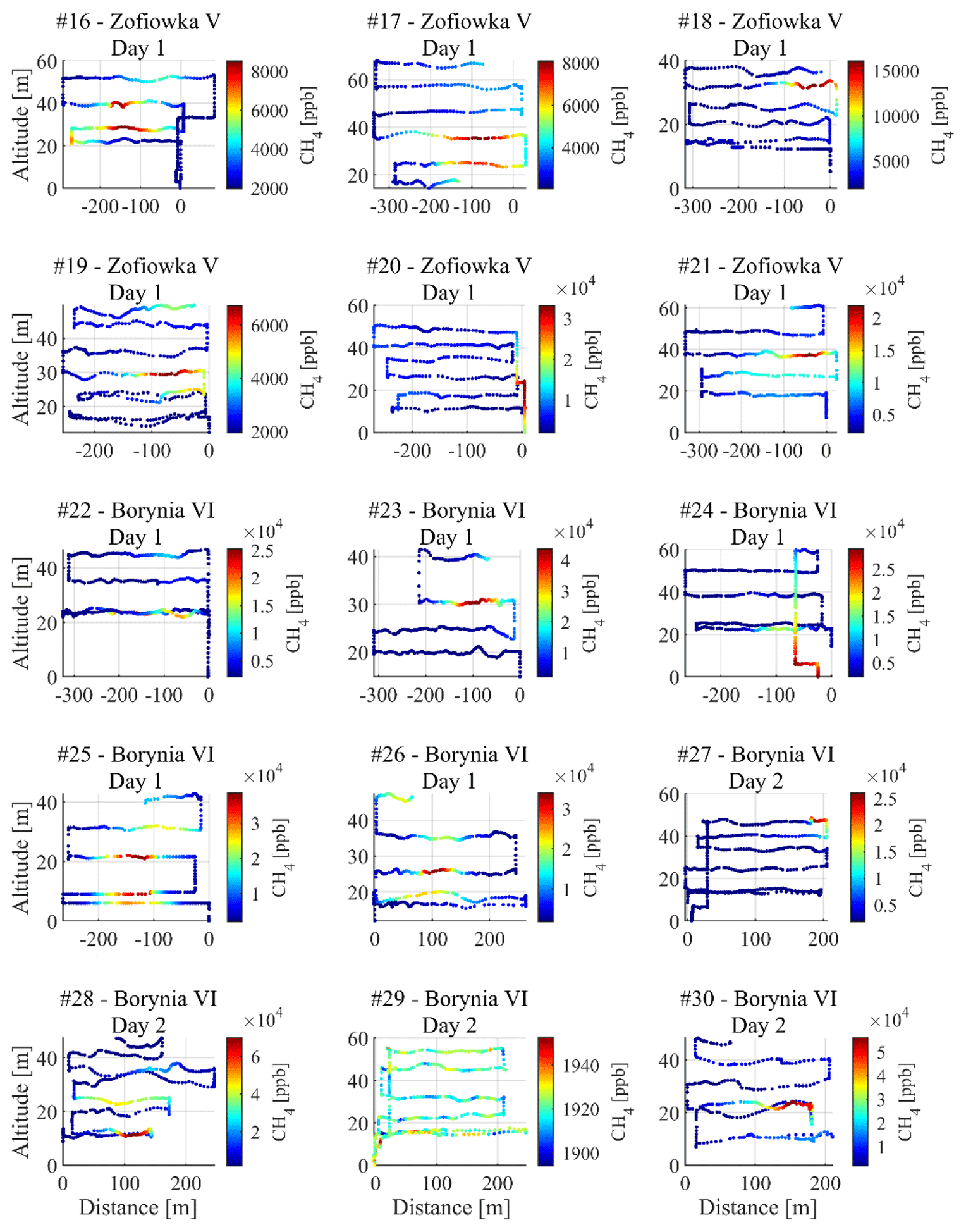
Figure A2The measured flight profiles for flight nos. 16 to 30. Flight nos. 20, 22, 23, 24, 25, 27, 28, and 29 are excluded according to the flight selection criteria.

Figure A3Measured flight profiles for flight nos. 31 to 45. Flight nos. 32, 33, 41, 42, 43, 44, and 45 are excluded according to the flight selection criteria.

Figure A4Measured flight profiles for flight nos. 46 to 59. Flight nos. 46, 47, 53, 55, 56, 57, and 59 are excluded according to the flight selection criteria.
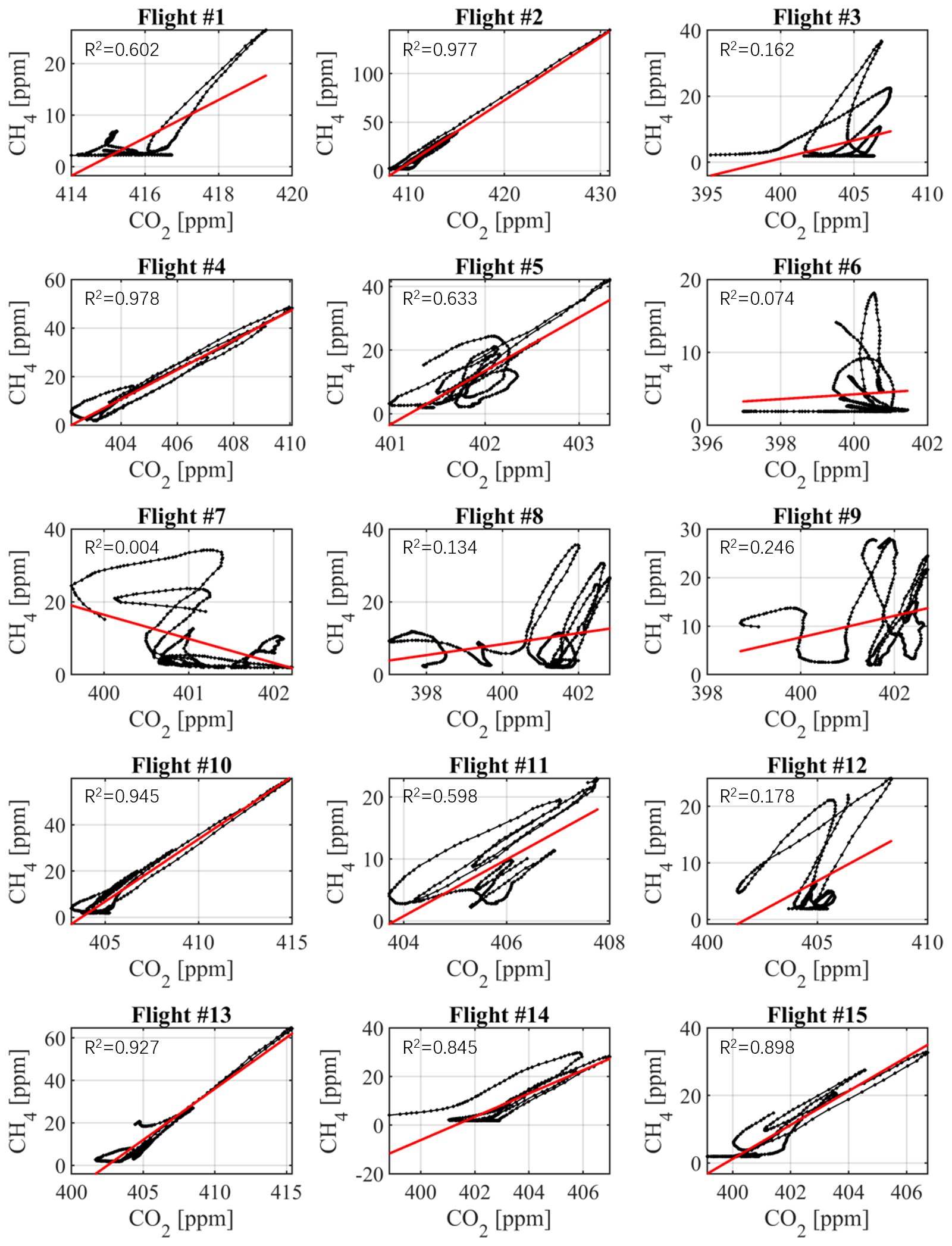
Figure B1Scatterplots for flight nos. 1 to 15. Flight nos. 2, 5, 10, 11, 14, and 15 are used to derive CO2 emissions fulfilling R2>0.5 and the flight selection criteria.
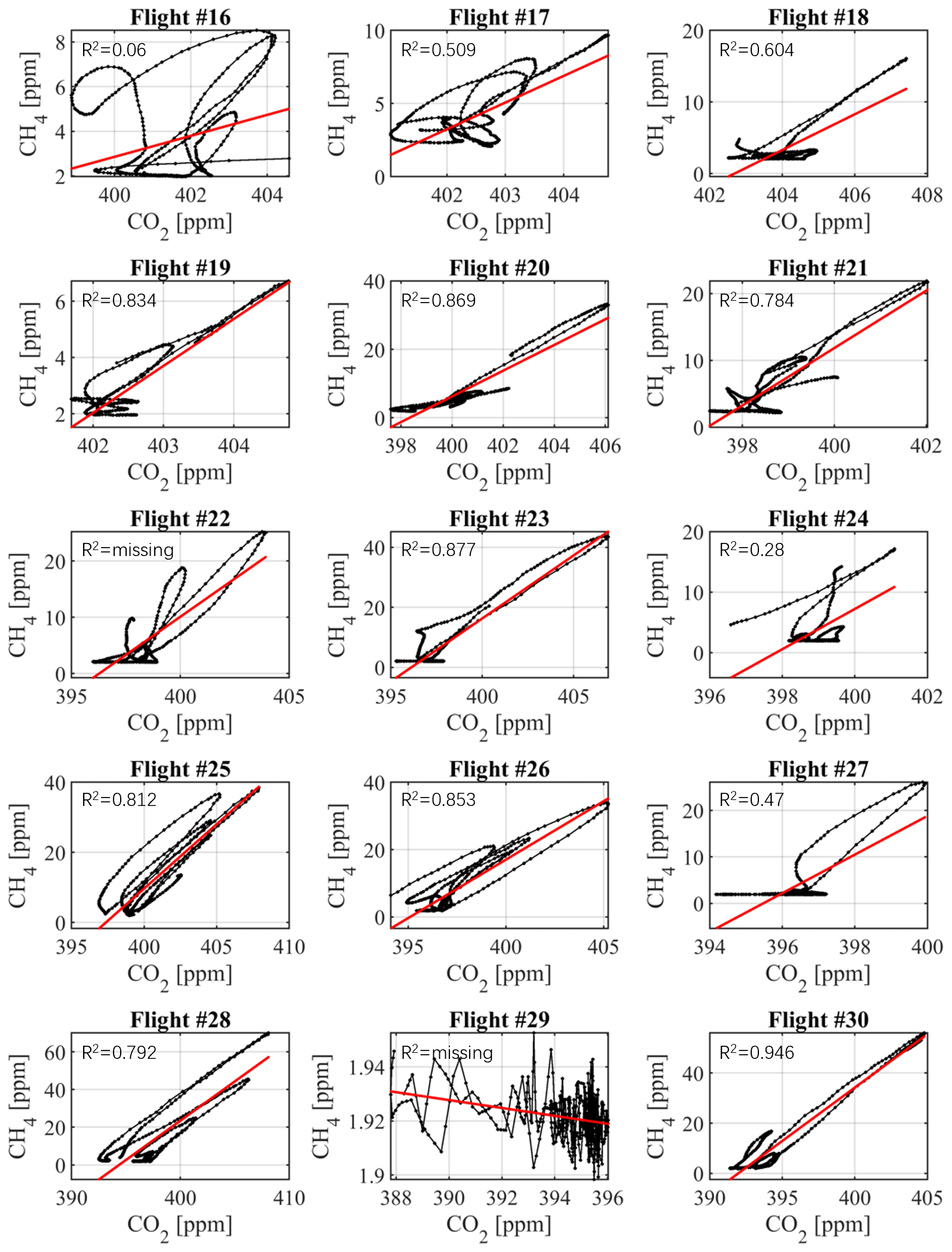
Figure B2Scatterplots for flights nos. 16 to 30. Flight nos. 17, 18, 19, 21, 26, and 30 are used to derive CO2 emissions fulfilling R2>0.5 and the flight selection criteria.
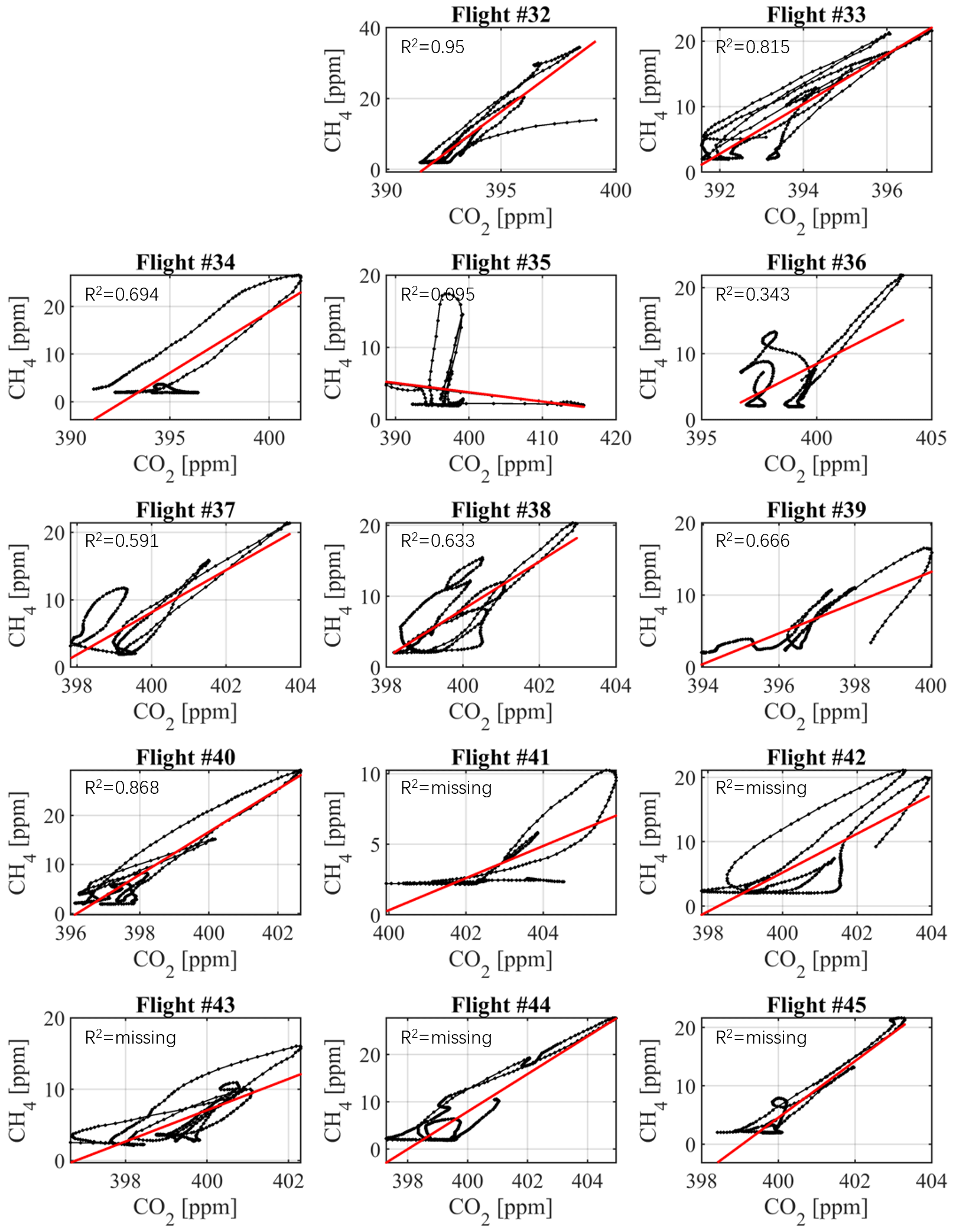
Figure B3Scatterplots for flight nos. 32 to 45. Flight nos. 34, 37, 38, 39, and 40 are used to derive CO2 emissions fulfilling R2>0.5 and the flight selection criteria. Flight no. 31 is missing because of the lack of CO2 information.
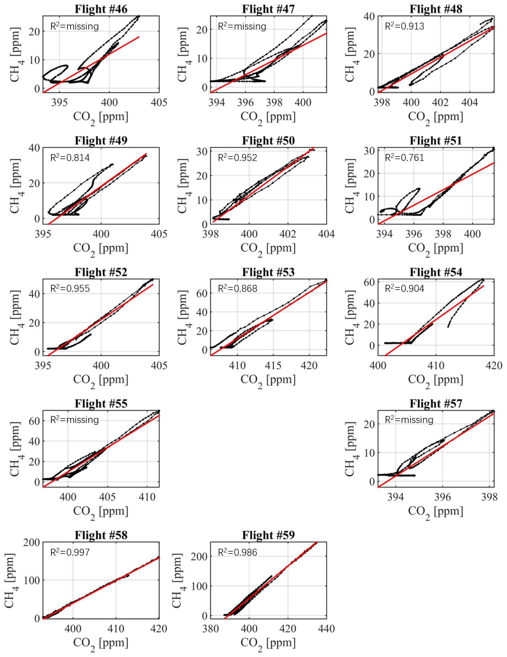
Figure B4Scatterplots for flight nos. 46 to 59. Flight nos. 48,49,50,51,52,53,54, and 58 are used to derive CO2 emissions fulfilling R2>0.5 and the flight selection criteria. Flight no. 56 is missing because of the lack of CO2 information.
Table C1The statistics for the annual CH4 inventory (E-PRTR, 2018), the hourly inventory during the days of flying, and the UAV-based active AirCore IG quantified CH4 emissions for each coal mine ventilation shaft.

The raw data sets and flight logs, as well as wind data from the period 18 May–1 June 2018, can be accessed at https://doi.org/10.5281/zenodo.5786532 (Andersen et al., 2021b).
HC, TA, and AR planned the campaign. TA, MdV, HC, and MM performed the measurements. TA and HC analyzed the data. TA and HC wrote the manuscript draft. WP, JN, JS, MM, TR, AR, AF, and ZZ reviewed and edited the manuscript.
The contact author has declared that none of the authors has any competing interests.
Publisher's note: Copernicus Publications remains neutral with regard to jurisdictional claims in published maps and institutional affiliations.
This article is part of the special issue “CoMet: a mission to improve our understanding and to better quantify the carbon dioxide and methane cycles”. It is not associated with a conference.
We would like to thank the CoMet project for the opportunity to participate in an exciting and stimulating campaign and collaborate with the participants of the campaign with tons of great discussions and good times.
This work was supported by the National Key Research and Development Program of China under grant no. 2022YFE0209100, and was funded by the MEthane goes Mobile: MEasurement and MOdeling (MEMO2) project from the European Union's Horizon 2020 research and innovation programme under the Marie Sklodowska-Curie grant agreement no. 722479. Furthermore, the research was supported by equipment financed from the funds of the “Excellence Initiative - Research University” program at AGH University of Science and Technology.
This paper was edited by Manvendra Krishna Dubey and reviewed by two anonymous referees.
Allen, G., Hollingsworth, P., Kabbabe, K., Pitt, J. R., Mead, M. I., Illingworth, S., Roberts, G., Bourn, M., Shallcross, D. E., and Percival, C. J.: The development and trial of an unmanned aerial system for the measurement of methane flux from landfill and greenhouse gas emission hotspots, Waste Manage., 87, 883–892, https://doi.org/10.1016/j.wasman.2017.12.024, 2019.
Andersen, T., Scheeren, B., Peters, W., and Chen, H.: A UAV-based active AirCore system for measurements of greenhouse gases, Atmos. Meas. Tech., 11, 2683–2699, https://doi.org/10.5194/amt-11-2683-2018, 2018.
Andersen, T., Vinkovic, K., de Vries, M., Kers, B., Necki, J., Swolkien, J., Roiger, A., Peters, W., and Chen, H.: Quantifying methane emissions from coal mining ventilation shafts using a small Unmanned Aerial Vehicle (UAV)-based active AirCore system, Atmos. Environ. X, 12, 100135, https://doi.org/10.1016/j.aeaoa.2021.100135, 2021a.
Andersen, T., de Vries, M., Necki, J., Swolkien, J., Menoud, M., Röckmann, T., Roiger, A., Fix, A., Peters, W., and Chen, H.: Local to regional methane emissions from the Upper Silesia Coal Basin (USCB) quantified using UAV-based atmospheric measurements (1.0), Zenodo [data set], https://doi.org/10.5281/zenodo.5786532, 2021b.
Andrews, A. E., Kofler, J. D., Trudeau, M. E., Williams, J. C., Neff, D. H., Masarie, K. A., Chao, D. Y., Kitzis, D. R., Novelli, P. C., Zhao, C. L., Dlugokencky, E. J., Lang, P. M., Crotwell, M. J., Fischer, M. L., Parker, M. J., Lee, J. T., Baumann, D. D., Desai, A. R., Stanier, C. O., De Wekker, S. F. J., Wolfe, D. E., Munger, J. W., and Tans, P. P.: CO2, CO, and CH4 measurements from tall towers in the NOAA Earth System Research Laboratory's Global Greenhouse Gas Reference Network: instrumentation, uncertainty analysis, and recommendations for future high-accuracy greenhouse gas monitoring efforts, Atmos. Meas. Tech., 7, 647–687, https://doi.org/10.5194/amt-7-647-2014, 2014.
Bell, C. S., Vaughn, T., and Zimmerle, D.: Evaluation of next generation emission measurement technologies under repeatable test protocols, Elementa–Sci. Anthrop., 8, 32, https://doi.org/10.1525/elementa.426, 2020.
Bonetti, B., Abruzzi, R. C., Peglow, C. P., Pires, M. J. R., and Gomes, C. J. B.: CH4 and CO2 monitoring in the air of underground coal mines in southern Brazil and GHG emission estimation, REM – International Engineering Journal, 72, 635–642, https://doi.org/10.1590/0370-44672018720105, 2019.
Brass, M. and Röckmann, T.: Continuous-flow isotope ratio mass spectrometry method for carbon and hydrogen isotope measurements on atmospheric methane, Atmos. Meas. Tech., 3, 1707–1721, https://doi.org/10.5194/amt-3-1707-2010, 2010.
Brosy, C., Krampf, K., Zeeman, M., Wolf, B., Junkermann, W., Schäfer, K., Emeis, S., and Kunstmann, H.: Simultaneous multicopter-based air sampling and sensing of meteorological variables, Atmos. Meas. Tech., 10, 2773–2784, https://doi.org/10.5194/amt-10-2773-2017, 2017.
Brownlow, R., Lowry, D., Thomas, R. M., Fisher, R. E., France, J. L., Cain, M., Richardson, T. S., Greatwood, C., Freer, J., Pyle, J. A., MacKenzie, A. R., and Nisbet, E. G.: Methane mole fraction and δ13C above and below the trade wind inversion at Ascension Island in air sampled by aerial robotics, Geophys. Res. Lett., 43, 11893–11902, https://doi.org/10.1002/2016gl071155, 2016.
Chang, C. C., Wang, J. L., Chang, C. Y., Liang, M. C., and Lin, M. R.: Development of a multicopter-carried whole air sampling apparatus and its applications in environmental studies, Chemosphere, 144, 484–492, https://doi.org/10.1016/j.chemosphere.2015.08.028, 2016.
Dlugokencky, E.: Trends in Atmospheric Methane, National Oceanic and Atmospheric Administration (NOAA)/Global Monitoring Laboratory (GML), https://gml.noaa.gov/ccgg/trends_ch4/, last access: 28 April 2023.
Ehret, G., Bousquet, P., Pierangelo, C., Alpers, M., Millet, B., Abshire, J. B., Bovensmann, H., Burrows, J. P., Chevallier, F., Ciais, P., Crevoisier, C., Fix, A., Flamant, P., Frankenberg, C., Gibert, F., Heim, B., Heimann, M., Houweling, S., Hubberten, H. W., Jöckel, P., Law, K., Löw, A., Marshall, J., Agusti-Panareda, A., Payan, S., Prigent, C., Rairoux, P., Sachs, T., Scholze, M., and Wirth, M.: MERLIN: A French-German space lidar mission dedicated to atmospheric methane, Remote Sens.-Basel, 9, 1052, https://doi.org/10.3390/rs9101052, 2017.
Etminan, M., Myhre, G., Highwood, E. J., and Shine, K. P.: Radiative forcing of carbon dioxide, methane, and nitrous oxide: A significant revision of the methane radiative forcing, Geophys. Res. Lett., 43, 12614–12623, https://doi.org/10.1002/2016gl071930, 2016.
Feitz, A., Schroder, I., Phillips, F., Coates, T., Negandhi, K., Day, S., Luhar, A., Bhatia, S., Edwards, G., Hrabar, S., Hernandez, E., Wood, B., Naylor, T., Kennedy, M., Hamilton, M., Hatch, M., Malos, J., Kochanek, M., Reid, P., Wilson, J., Deutscher, N., Zegelin, S., Vincent, R., White, S., Ong, C., George, S., Maas, P., Towner, S., Wokker, N., and Griffith, D.: The Ginninderra CH4 and CO2 release experiment: An evaluation of gas detection and quantification techniques, Int. J. Greenh. Gas Con., 70, 202–224, https://doi.org/10.1016/j.ijggc.2017.11.018, 2018.
Fiehn, A., Kostinek, J., Eckl, M., Klausner, T., Gałkowski, M., Chen, J., Gerbig, C., Röckmann, T., Maazallahi, H., Schmidt, M., Korbeń, P., Neçki, J., Jagoda, P., Wildmann, N., Mallaun, C., Bun, R., Nickl, A.-L., Jöckel, P., Fix, A., and Roiger, A.: Estimating CH4, CO2 and CO emissions from coal mining and industrial activities in the Upper Silesian Coal Basin using an aircraft-based mass balance approach, Atmos. Chem. Phys., 20, 12675–12695, https://doi.org/10.5194/acp-20-12675-2020, 2020.
Fix, A., Amediek, A., Bovensmann, H., Ehret, G., Gerbig, C., Gerilowski, K., Pfeilsticker, K., Roiger, A., and Zöger, M.: CoMet: an airborne mission to simultaneously measure CO2 and CH4 using lidar, passive remote sensing, and in-situ techniques, EPJ Web Conf., 176, 1–4, https://doi.org/10.1051/epjconf/201817602003, 2018.
Gałkowski, M., Fiehn, A., Swolkien, J., Stanisavljevic, M., Korben, P., Menoud, M., Necki, J., Roiger, A., Röckmann, T., Gerbig, C., and Fix, A.: Emissions of CH4 and CO2 over the Upper Silesian Coal Basin (Poland) and its vicinity (4.01), ICOS ERIC – Carbon Portal [data set], https://doi.org/10.18160/3K6Z-4H73, 2021.
Greatwood, C., Richardson, T. S., Freer, J., Thomas, R. M., MacKenzie, A. R., Brownlow, R., Lowry, D., Fisher, R. E., and Nisbet, E. G.: Atmospheric sampling on Ascension island using multirotor UAVs, Sensors, 17, 1189, https://doi.org/10.3390/s17061189, 2017.
Hannun, R. A., Wolfe, G. M., Kawa, S. R., Hanisco, T. F., Newman, P. A., Alfieri, J. G., Barrick, J., Clark, K. L., DiGangi, J. P., Diskin, G. S., King, J., Kustas, W. P., Mitra, B., Noormets, A., Nowak, J. B., Thornhill, K. L., and Vargas, R.: Spatial heterogeneity in CO2, CH4, and energy fluxes: insights from airborne eddy covariance measurements over the Mid-Atlantic region, Environ. Res. Lett., 15, 035008, https://doi.org/10.1088/1748-9326/ab7391, 2020.
Karion, A., Sweeney, C., Petron, G., Frost, G., Hardesty, R. M., Kofler, J., Miller, B. R., Newberger, T., Wolter, S., Banta, R., Brewer, A., Dlugokencky, E., Lang, P., Montzka, S. A., Schnell, R., Tans, P., Trainer, M., Zamora, R., and Conley, S.: Methane emissions estimate from airborne measurements over a western United States natural gas field, Geophys. Res. Lett., 40, 4393–4397, https://doi.org/10.1002/grl.50811, 2013.
Kirschke, S., Bousquet, P., Ciais, P., Saunois, M., Canadell, J. G., Dlugokencky, E. J., Bergamaschi, P., Bergmann, D., Blake, D. R., Bruhwiler, L., Cameron-Smith, P., Castaldi, S., Chevallier, F., Feng, L., Fraser, A., Heimann, M., Hodson, E. L., Houweling, S., Josse, B., Fraser, P. J., Krummel, P. B., Lamarque, J.-F., Langenfelds, R. L., Le Quere, C., Naik, V., O'Doherty, S., Palmer, P. I., Pison, I., Plummer, D., Poulter, B., Prinn, R. G., Rigby, M., Ringeval, B., Santini, M., Schmidt, M., Shindell, D. T., Simpson, I. J., Spahni, R., Steele, L. P., Strode, S. A., Sudo, K., Szopa, S., van der Werf, G. R., Voulgarakis, A., van Weele, M., Weiss, R. F., Williams, J. E., and Zeng, G.: Three decades of global methane sources and sinks, Nat. Geosci., 6, 813–823, https://doi.org/10.1038/ngeo1955, 2013.
Kostinek, J., Roiger, A., Eckl, M., Fiehn, A., Luther, A., Wildmann, N., Klausner, T., Fix, A., Knote, C., Stohl, A., and Butz, A.: Estimating Upper Silesian coal mine methane emissions from airborne in situ observations and dispersion modeling, Atmos. Chem. Phys., 21, 8791–8807, https://doi.org/10.5194/acp-21-8791-2021, 2021.
Krautwurst, S., Gerilowski, K., Jonsson, H. H., Thompson, D. R., Kolyer, R. W., Iraci, L. T., Thorpe, A. K., Horstjann, M., Eastwood, M., Leifer, I., Vigil, S. A., Krings, T., Borchardt, J., Buchwitz, M., Fladeland, M. M., Burrows, J. P., and Bovensmann, H.: Methane emissions from a Californian landfill, determined from airborne remote sensing and in situ measurements, Atmos. Meas. Tech., 10, 3429–3452, https://doi.org/10.5194/amt-10-3429-2017, 2017.
Kunz, M., Lavric, J. V., Gasche, R., Gerbig, C., Grant, R. H., Koch, F.-T., Schumacher, M., Wolf, B., and Zeeman, M.: Surface flux estimates derived from UAS-based mole fraction measurements by means of a nocturnal boundary layer budget approach, Atmos. Meas. Tech., 13, 1671–1692, https://doi.org/10.5194/amt-13-1671-2020, 2020.
Lampert, A., Pätzold, F., Asmussen, M. O., Lobitz, L., Krüger, T., Rausch, T., Sachs, T., Wille, C., Sotomayor Zakharov, D., Gaus, D., Bansmer, S., and Damm, E.: Studying boundary layer methane isotopy and vertical mixing processes at a rewetted peatland site using an unmanned aircraft system, Atmos. Meas. Tech., 13, 1937–1952, https://doi.org/10.5194/amt-13-1937-2020, 2020.
Lan, X., Basu, S., Schwietzke, S., Bruhwiler, L. M. P., Dlugokencky, E. J., Michel, S. E., Sherwood, O. A., Tans, P. P., Thoning, K., Etiope, G., Zhuang, Q., Liu, L., Oh, Y., Miller, J. B., Pétron, G., Vaughn, B. H., and Crippa, M.: Improved Constraints on Global Methane Emissions 460 and Sinks Using Δ13C-CH4, Global Biogeochem. Cy., 35, 007000, https://doi.org/10.1029/2021GB007000, 2021.
Lowry, D., Brownlow, R., Fisher, R., Nisbet, E., Lanoisellé, M., France, J., Thomas, R., Mackenzie, R., Richardson, T., Greatwood, C., Freer, J., Cain, M., Warwick, N., and Pyle, J.: Methane at ascension island, southern tropical Atlantic Ocean: continuous ground measurement and vertical profiling above the trade-wind inversion, EGU General Assembly 2015, Vienna, Austria, 12–17 April 2015, EGU2015-7100, 2015.
Martinez, B., Miller, T. W., and Yalin, A. P.: Cavity ring-down methane sensor for small unmanned aerial systems, Sensors, 20, 454, https://doi.org/10.3390/s20020454, 2020.
Menoud, M., Röckmann, T., Fernandez, J., Bakkaloglu, S., Lowry, D., Korben, P., Schmidt, M., Stanisavljevic, M., Necki, J., Defratyka, S., and Yver Kwok, C.: mamenoud/MEMO2_isotopes: v8.1 complete (Version v8.1.0), Zenodo [data set], https://doi.org/10.5281/zenodo.4062356, 2020.
Menoud, M., van der Veen, C., Necki, J., Bartyzel, J., Szénási, B., Stanisavljević, M., Pison, I., Bousquet, P., and Röckmann, T.: Methane (CH4) sources in Krakow, Poland: insights from isotope analysis, Atmos. Chem. Phys., 21, 13167–13185, https://doi.org/10.5194/acp-21-13167-2021, 2021.
Morales, R., Ravelid, J., Vinkovic, K., Korbeń, P., Tuzson, B., Emmenegger, L., Chen, H., Schmidt, M., Humbel, S., and Brunner, D.: Controlled-release experiment to investigate uncertainties in UAV-based emission quantification for methane point sources, Atmos. Meas. Tech., 15, 2177–2198, https://doi.org/10.5194/amt-15-2177-2022, 2022.
Nathan, B. J., Golston, L. M., O'Brien, A. S., Ross, K., Harrison, W. A., Tao, L., Lary, D. J., Johnson, D. R., Covington, A. N., Clark, N. N., and Zondlo, M. A.: Near-field characterization of methane emission variability from a compressor station using a model aircraft, Environ. Sci. Technol., 49, 7896–7903, https://doi.org/10.1021/acs.est.5b00705, 2015.
Nickl, A.-L., Mertens, M., Roiger, A., Fix, A., Amediek, A., Fiehn, A., Gerbig, C., Galkowski, M., Kerkweg, A., Klausner, T., Eckl, M., and Jöckel, P.: Hindcasting and forecasting of regional methane from coal mine emissions in the Upper Silesian Coal Basin using the online nested global regional chemistry–climate model MECO(n) (MESSy v2.53), Geosci. Model Dev., 13, 1925–1943, https://doi.org/10.5194/gmd-13-1925-2020, 2020.
Ražnjević, A., van Heerwaarden, C., van Stratum, B., Hensen, A., Velzeboer, I., van den Bulk, P., and Krol, M.: Technical note: Interpretation of field observations of point-source methane plume using observation-driven large-eddy simulations, Atmos. Chem. Phys., 22, 6489–6505, https://doi.org/10.5194/acp-22-6489-2022, 2022.
Röckmann, T., Eyer, S., van der Veen, C., Popa, M. E., Tuzson, B., Monteil, G., Houweling, S., Harris, E., Brunner, D., Fischer, H., Zazzeri, G., Lowry, D., Nisbet, E. G., Brand, W. A., Necki, J. M., Emmenegger, L., and Mohn, J.: In situ observations of the isotopic composition of methane at the Cabauw tall tower site, Atmos. Chem. Phys., 16, 10469–10487, https://doi.org/10.5194/acp-16-10469-2016, 2016.
Satar, E., Berhanu, T. A., Brunner, D., Henne, S., and Leuenberger, M.: Continuous measurements (2012–2014) at Beromünster tall tower station in Switzerland, Biogeosciences, 13, 2623–2635, https://doi.org/10.5194/bg-13-2623-2016, 2016.
Saunois, M., Bousquet, P., Poulter, B., Peregon, A., Ciais, P., Canadell, J. G., Dlugokencky, E. J., Etiope, G., Bastviken, D., Houweling, S., Janssens-Maenhout, G., Tubiello, F. N., Castaldi, S., Jackson, R. B., Alexe, M., Arora, V. K., Beerling, D. J., Bergamaschi, P., Blake, D. R., Brailsford, G., Brovkin, V., Bruhwiler, L., Crevoisier, C., Crill, P., Covey, K., Curry, C., Frankenberg, C., Gedney, N., Höglund-Isaksson, L., Ishizawa, M., Ito, A., Joos, F., Kim, H.-S., Kleinen, T., Krummel, P., Lamarque, J.-F., Langenfelds, R., Locatelli, R., Machida, T., Maksyutov, S., McDonald, K. C., Marshall, J., Melton, J. R., Morino, I., Naik, V., O'Doherty, S., Parmentier, F.-J. W., Patra, P. K., Peng, C., Peng, S., Peters, G. P., Pison, I., Prigent, C., Prinn, R., Ramonet, M., Riley, W. J., Saito, M., Santini, M., Schroeder, R., Simpson, I. J., Spahni, R., Steele, P., Takizawa, A., Thornton, B. F., Tian, H., Tohjima, Y., Viovy, N., Voulgarakis, A., van Weele, M., van der Werf, G. R., Weiss, R., Wiedinmyer, C., Wilton, D. J., Wiltshire, A., Worthy, D., Wunch, D., Xu, X., Yoshida, Y., Zhang, B., Zhang, Z., and Zhu, Q.: The global methane budget 2000–2012, Earth Syst. Sci. Data, 8, 697–751, https://doi.org/10.5194/essd-8-697-2016, 2016a.
Saunois, M., Jackson, R. B., Bousquet, P., Poulter, B., and Canadell, J. G.: The growing role of methane in anthropogenic climate change, Environ. Res. Lett., 11, 120207, https://doi.org/10.1088/1748-9326/11/12/120207, 2016b.
Saunois, M., Bousquet, P., Poulter, B., Peregon, A., Ciais, P., Canadell, J. G., Dlugokencky, E. J., Etiope, G., Bastviken, D., Houweling, S., Janssens-Maenhout, G., Tubiello, F. N., Castaldi, S., Jackson, R. B., Alexe, M., Arora, V. K., Beerling, D. J., Bergamaschi, P., Blake, D. R., Brailsford, G., Bruhwiler, L., Crevoisier, C., Crill, P., Covey, K., Frankenberg, C., Gedney, N., Höglund-Isaksson, L., Ishizawa, M., Ito, A., Joos, F., Kim, H.-S., Kleinen, T., Krummel, P., Lamarque, J.-F., Langenfelds, R., Locatelli, R., Machida, T., Maksyutov, S., Melton, J. R., Morino, I., Naik, V., O'Doherty, S., Parmentier, F.-J. W., Patra, P. K., Peng, C., Peng, S., Peters, G. P., Pison, I., Prinn, R., Ramonet, M., Riley, W. J., Saito, M., Santini, M., Schroeder, R., Simpson, I. J., Spahni, R., Takizawa, A., Thornton, B. F., Tian, H., Tohjima, Y., Viovy, N., Voulgarakis, A., Weiss, R., Wilton, D. J., Wiltshire, A., Worthy, D., Wunch, D., Xu, X., Yoshida, Y., Zhang, B., Zhang, Z., and Zhu, Q.: Variability and quasi-decadal changes in the methane budget over the period 2000–2012, Atmos. Chem. Phys., 17, 11135–11161, https://doi.org/10.5194/acp-17-11135-2017, 2017.
Saunois, M., Stavert, A. R., Poulter, B., Bousquet, P., Canadell, J. G., Jackson, R. B., Raymond, P. A., Dlugokencky, E. J., Houweling, S., Patra, P. K., Ciais, P., Arora, V. K., Bastviken, D., Bergamaschi, P., Blake, D. R., Brailsford, G., Bruhwiler, L., Carlson, K. M., Carrol, M., Castaldi, S., Chandra, N., Crevoisier, C., Crill, P. M., Covey, K., Curry, C. L., Etiope, G., Frankenberg, C., Gedney, N., Hegglin, M. I., Höglund-Isaksson, L., Hugelius, G., Ishizawa, M., Ito, A., Janssens-Maenhout, G., Jensen, K. M., Joos, F., Kleinen, T., Krummel, P. B., Langenfelds, R. L., Laruelle, G. G., Liu, L., Machida, T., Maksyutov, S., McDonald, K. C., McNorton, J., Miller, P. A., Melton, J. R., Morino, I., Müller, J., Murguia-Flores, F., Naik, V., Niwa, Y., Noce, S., O'Doherty, S., Parker, R. J., Peng, C., Peng, S., Peters, G. P., Prigent, C., Prinn, R., Ramonet, M., Regnier, P., Riley, W. J., Rosentreter, J. A., Segers, A., Simpson, I. J., Shi, H., Smith, S. J., Steele, L. P., Thornton, B. F., Tian, H., Tohjima, Y., Tubiello, F. N., Tsuruta, A., Viovy, N., Voulgarakis, A., Weber, T. S., van Weele, M., van der Werf, G. R., Weiss, R. F., Worthy, D., Wunch, D., Yin, Y., Yoshida, Y., Zhang, W., Zhang, Z., Zhao, Y., Zheng, B., Zhu, Q., Zhu, Q., and Zhuang, Q.: The Global Methane Budget 2000–2017, Earth Syst. Sci. Data, 12, 1561–1623, https://doi.org/10.5194/essd-12-1561-2020, 2020.
Shah, A., Pitt, J. R., Ricketts, H., Leen, J. B., Williams, P. I., Kabbabe, K., Gallagher, M. W., and Allen, G.: Testing the near-field Gaussian plume inversion flux quantification technique using unmanned aerial vehicle sampling, Atmos. Meas. Tech., 13, 1467–1484, https://doi.org/10.5194/amt-13-1467-2020, 2020.
Sherwood, O. A., Schwietzke, S., and Lan, X.: Global δ13C-CH4 Source Signature Inventory 2020, NOAA Global Monitoring Laboratory Data Repository [data set], https://doi.org/10.15138/qn55-e011, 2021
Shi, T., Han, Z., Han, G., Ma, X., Chen, H., Andersen, T., Mao, H., Chen, C., Zhang, H., and Gong, W.: Retrieving CH4-emission rates from coal mine ventilation shafts using UAV-based AirCore observations and the genetic algorithm–interior point penalty function (GA-IPPF) model, Atmos. Chem. Phys., 22, 13881–13896, https://doi.org/10.5194/acp-22-13881-2022, 2022.
Stanisavljević, M.: Determination of methane (CH4) emission rates and its origin from selected areas of mining exploitation in Poland and Germany, PhD thesis, AGH University of Science and Technology, Poland, 157 pp., 2021.
Swolkień, J.: Polish underground coal mines as point sources of methane emission to the atmosphere, Int. J. Greenh. Gas Con., 94, 102921, https://doi.org/10.1016/j.ijggc.2019.102921, 2020.
Turnbull, J. C., Keller, E. D., Baisden, T., Brailsford, G., Bromley, T., Norris, M., and Zondervan, A.: Atmospheric measurement of point source fossil CO2 emissions, Atmos. Chem. Phys., 14, 5001–5014, https://doi.org/10.5194/acp-14-5001-2014, 2014.
Turner, A. J., Frankenberg, C., and Kort, E. A.: Interpreting contemporary trends in atmospheric methane, P. Natl. Acad. Sci. USA, 116, 2805–2813, https://doi.org/10.1073/pnas.1814297116, 2019.
Tuzson, B., Graf, M., Ravelid, J., Scheidegger, P., Kupferschmid, A., Looser, H., Morales, R. P., and Emmenegger, L.: A compact QCL spectrometer for mobile, high-precision methane sensing aboard drones, Atmos. Meas. Tech., 13, 4715–4726, https://doi.org/10.5194/amt-13-4715-2020, 2020.
Van Dingenen, R., Crippa, M., Maenhout, G., Guizzardi, D., and Dentener, F.: Global trends of methane emissions and their impacts on ozone concentrations, Tech. rep., EUR 29394 EN, Publications Office of the European Union, Luxembourg, ISBN 978-92-79-96550-0, 2018.
Villa, T. F., Gonzalez, F., Miljievic, B., Ristovski, Z. D., and Morawska, L.: An overview of small unmanned aerial vehicles for air quality measurements: Present applications and future prospectives, Sensors, 16, 1072, https://doi.org/10.3390/s16071072, 2016.
Vinković, K., Andersen, T., De Vries, M., Kers, B., Van Heuven, S., Peters, W., Hensen, A., Den Bulk, P., and Chen, H.: Evaluating the use of an Unmanned Aerial Vehicle (UAV)-based active AirCore system to quantify methane emissions from dairy cows, Sci. Total Environ., 831, 154898, https://doi.org/10.1016/j.scitotenv.2022.154898, 2022.
Werner, C., Davis, K., Bakwin, P., Yi, C. X., Hurst, D., and Lock, L.: Regional-scale measurements of CH4 exchange from a tall tower over a mixed temperate/boreal lowland and wetland forest, Glob. Change Biol., 9, 1251–1261, https://doi.org/10.1046/j.1365-2486.2003.00670.x, 2003.
Zazzeri, G., Lowry, D., Fisher, R. E., France, J. L., Lanoisellé, M., Kelly, B. F. J., Necki, J. M., Iverach, C. P., Ginty, E., Zimnoch, M., Jasek, A., and Nisbet, E. G.: Carbon isotopic signature of coal-derived methane emissions to the atmosphere: from coalification to alteration, Atmos. Chem. Phys., 16, 13669–13680, https://doi.org/10.5194/acp-16-13669-2016, 2016.
- Abstract
- Introduction
- Methodology
- Results and discussion
- Conclusions and outlook
- Appendix A: Flight profiles
- Appendix B: Scatterplots of CH4 and CO2
- Appendix C: Inventory and UAV-quantified emissions rates of the five ventilation shafts
- Data availability
- Author contributions
- Competing interests
- Disclaimer
- Special issue statement
- Acknowledgements
- Financial support
- Review statement
- References