Identifying and accounting for the Coriolis effect in satellite NO₂ observations and emission estimates

Recent developments in atmospheric remote sensing from satellites have made it possible to resolve daily emission plumes from industrial point sources around the globe. Wind rotation aggregation coupled with statistical fitting is commonly used to extract emission estimates from these observations. These methods are used here to investigate how the Coriolis effect influences the trajectory of observed emission plumes as well as to assess the impact of this influence on satellite-derived emission estimates. Of the 16 industrial sites investigated, 9 showed the expected curvature for the hemisphere that they reside in, 5 showed no or negligible curvature, and 2 showed opposing or unusual curvature. The sites that showed conflicting curvature reside in topographically diverse regions, where strong meso-γ-scale (2–20 km) turbulence dominates over larger synoptic circulation patterns. For high-curvature cases, the assumption that the wind-rotated plume aggregate is symmetrically distributed across the downwind axis breaks down, which impairs the quality of statistical fitting procedures. Using annual NO_x emissions from Matimba power station as a test case, not compensating for Coriolis curvature resulted in an underestimation of ∼ 9 % on average for the years 2018 to 2021. This study is the first formal observation of the Coriolis effect and its influence on satellite-derived emission estimates, and it highlights both the variability in the emission calculation methods and the need for a standardised scheme for these data to act as evidence for regulators.

1 Introduction

For the past 3 decades, national space agencies and private industry have been launching satellite-based instruments to monitor and evaluate atmospheric composition, atmospheric chemistry, and anthropogenic emissions around the world. These instruments use absorption-based spectroscopy and interferometry to derive column counts of potentially harmful pollutants, and they have enhanced our understanding of the impact that these species have on air quality and the environment. New high-resolution instruments, such as the TROPOspheric Monitoring Instrument (TROPOMI), can resolve emission plumes from large industrial point sources, such as power generation, industrial fabrication, and oil refining processes (Anema, 2021; Goldberg et al., 2019; Ialongo et al., 2021; Wang et al., 2022). A suite of methods have been developed to derive emission estimates from both daily and time-aggregated observations of these large sources (Beirle et al., 2011, 2019; de Foy et al., 2015; Fioletov et al., 2015; Hakkarainen et al., 2021), providing a potential avenue for these instruments to assist with regulation and to constrain bottom-up emission estimates (Marais et al., 2021; Pope et al., 2022; Potts et al., 2021). Emissions from these sources are often distinct, thermally buoyant, and can extend over 0–20 km vertically and 10–200 km horizontally, where large-scale atmospheric effects may progressively influence the dispersion and trajectory of the plume as it travels downwind. Here, we investigate the influence of the Coriolis effect on large industrial emission plumes using observations of nitrogen dioxide (NO₂) from TROPOMI and explore the impact of Coriolis-induced curvature, plume geometry, and wind fields on satellite-derived emission estimates from large point sources.

2 Data and methods

2.1 TROPOMI NO₂

TROPOMI was launched by the European Space Agency (ESA) in October 2017 aboard the Sentinel-5 Precursor (S5P) satellite. TROPOMI is a nadir-viewing (downward-facing) short-wave spectrometer, observing in the ultraviolet–visible (UV–Vis, 270–500 nm), near-infrared (NIR, 710–770 nm), and short-wave infrared (SWIR, 2314–2382 nm) ranges (Veefkind et al., 2012). It has a spatial resolution of 5.5 × 3.5 km at nadir (7 × 5.5 km for SWIR) and a revisit time of around 13:30 LT (local time) each day. TROPOMI data products include, but are not limited to, nitrogen dioxide (NO₂), sulfur dioxide (SO₂), carbon monoxide (CO), methane (CH₄), and ozone (O₃), each with varying sensitivity, resolution, and precision. For this study, tropospheric NO₂ from TROPOMI is used because it has a comparatively short photochemical lifetime of 2–24 h (Beirle et al., 2011; Shah et al., 2020; Valin et al., 2013), so elevated tropospheric column counts are usually strongly correlated spatially with the emitting point source. This correlation enables more accurate source attribution and plume isolation for emissions from anthropogenic sources, such as large industry and populous urban environments (Goldberg et al., 2020), compared with other longer-lived pollutants. The TROPOMI processor upgraded to version 2.2.0 in July 2021, which resulted in a 10 %–15 % increase in tropospheric column NO₂, particularly over polluted scenes with small cloud fractions (Eskes et al., 2019). Here, the S5P-PAL product has been used, in which observations before July 2021 have been reprocessed with the v2.2.0 processor to achieve a better retrieval and to ensure consistency across the time frame, thereby harmonising the dataset. For this study, data from May 2018 to November 2021 were used, and observations have been oversampled onto a 0.01^∘ × 0.01^∘ regular grid, following the subpixel sampling approach of Pope et al. (2018). A quality flag of 0.75 was used, as per the S5P NO₂ user manual (Eskes et al., 2019), which filters out cloud-contaminated pixels and poor-quality retrievals. Furthermore, at least 75 % of the possible pixels within a region around the source were required to pass the quality filter for that daily observation to be included in the aggregate. For each observation, this region was defined as ±20 km from the site perpendicular to the wind direction and from −20 to +60 km along the wind direction; this discarded observations where there was not sufficient coverage over the downwind region. The number of observations included in each aggregate is annotated on the figures as “n”.

2.2 Site selection

In order to explore the impact of the Coriolis effect on wind rotation aggregation, several sites were investigated. Selection was based on latitude and the following three additional criteria: (1) sites 50 km from any large urban or industrial source, in order to avoid overlap of multiple plumes; (2) sites of a sufficient size to produce a plume that can be detected by TROPOMI, generally >1000 MW capacity for a power station (note that higher capacity does not equate directly to higher emissions); and (3) sites in operation during the 2018–present operational lifetime of TROPOMI. Sites were identified from the Global Power Plant Database (2018) and the point source emission catalogue developed by Beirle et al. (2021). In total 16 sites were investigated, and their details are outlined in Table 1. A total of 15 sites were coal- or oil-fired power stations, in order to allow for more direct comparisons. The remaining site is a large copper mining/smelting operation.

Table 1 Coordinates and plant information for the locations investigated in the study.

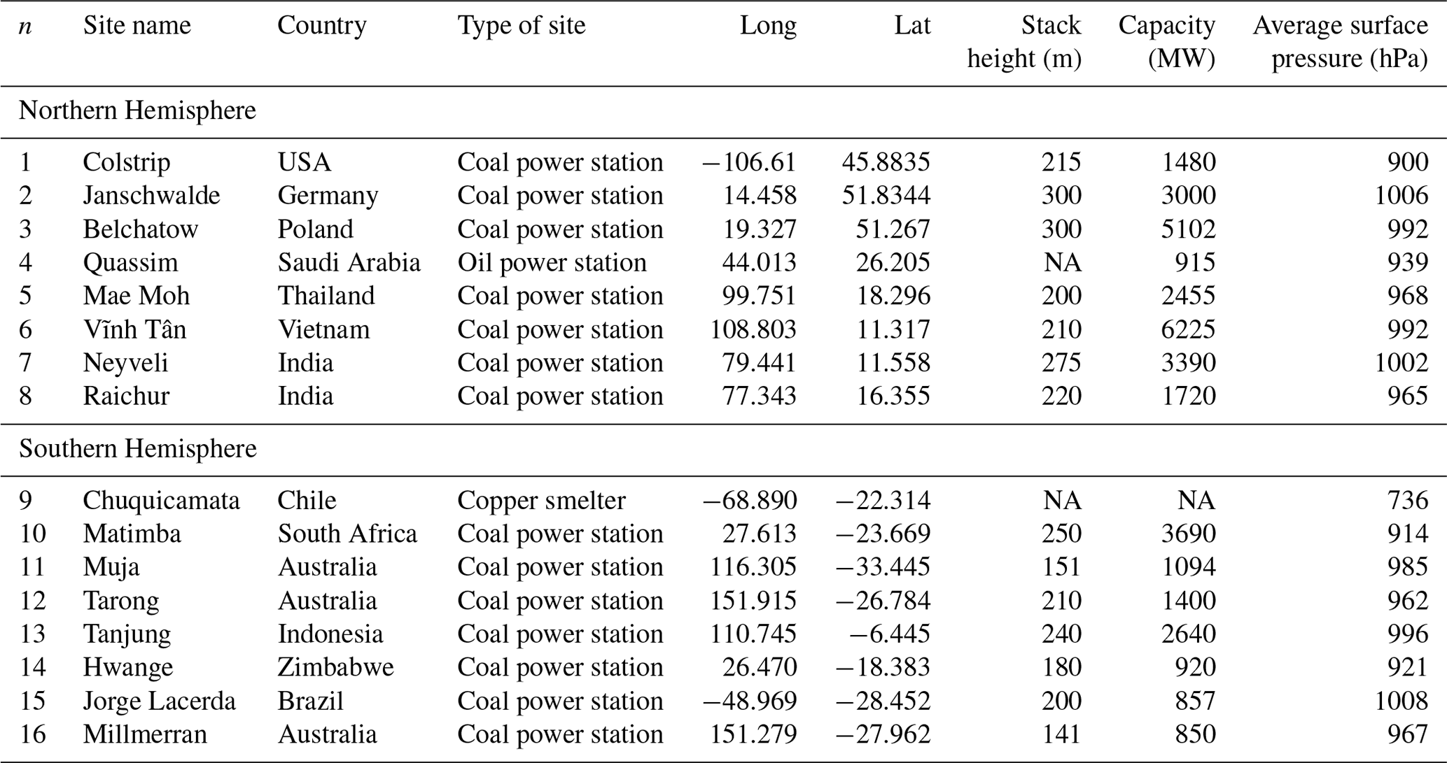
NA stands for not available.

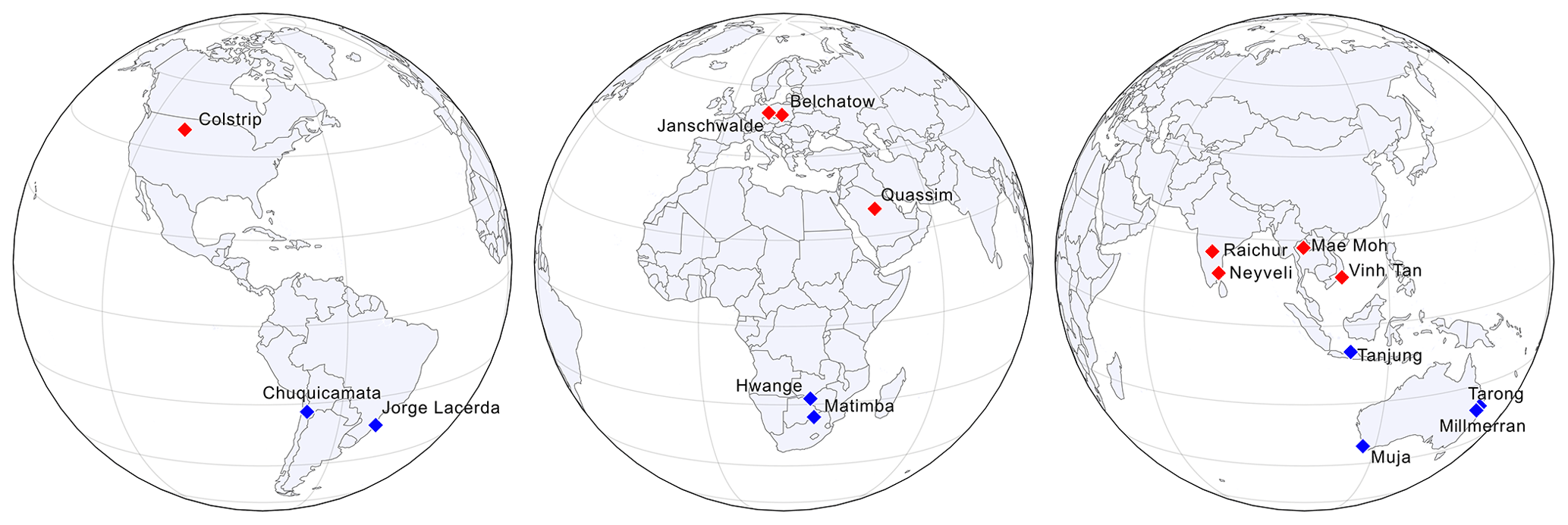
Figure 1 Locations of the sites used in the investigation. Northern Hemisphere sites are shown in red, and Southern Hemisphere sites are shown in blue.

2.3 Wind rotation aggregation

Wind rotation aggregation is a well-established method for combining multiple observations whilst preserving the structure of an emission plume. Pioneered by Pommier et al. (2013), this approach has been used for various satellite-based studies of point source emissions, such as cities (Goldberg et al., 2019), power stations (Fioletov et al., 2015; Hakkarainen et al., 2021), fertiliser plants (Clarisse et al., 2019; Dammers et al., 2019), and oil refineries (Potts et al., 2021). Each observation that passes quality filtering requirements (Fig. 2a) is rotated so that the wind vector is aligned to a predetermined axis, in this case in the west–east direction (Fig. 2b). This process is repeated for every observation that passes quality filtering requirements to produce the wind-rotated aggregate (Fig. 2c). The angle of rotation is found from the angle that the wind vector at the origin/industrial site makes with the chosen axis of rotation. The entire observation is rotated through this angle to achieve alignment. This is done using Eq. (1), where long_i and lat_i are the coordinates of each pixel corner in the observation, and the angle between the wind vector and the east direction is θ_wind. This allows for all quality data to be used and preserves the upwind–downwind profile of the emission plume (de Foy et al., 2015; Fioletov et al., 2015).

$$\begin{array}{}\text{(1)}& {\displaystyle \frac{{\mathrm{long}}_i^{\prime }}{{\mathrm{lat}}_i^{\prime }}}=\left(\begin{array}{ll}\cos {\mathit{\theta }}_{\mathrm{wind}}& -\sin {\mathit{\theta }}_{\mathrm{wind}}\\ \sin {\mathit{\theta }}_{\mathrm{wind}}& \cos {\mathit{\theta }}_{\mathrm{wind}}\end{array}\right){\displaystyle \frac{{\mathrm{long}}_i}{{\mathrm{lat}}_i}}\end{array}$$

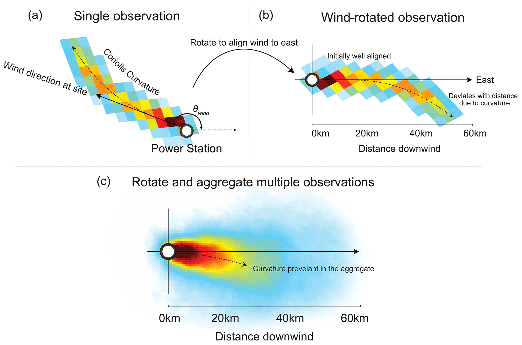
Figure 2 Illustration of the wind rotation method. Panel (a) presents a single overpass from TROPOMI for Belchatow power station on 3 June 2019. In panel (b), the plume is rotated so that its wind vector now points eastwards. This initial stage of the plume is well aligned, but Coriolis curvature causes the latter parts of the plume to deviate from the downwind x axis. In panel (c), this rotational process is repeated for all quality observations and aggregated into a wind-rotated average. On average the Coriolis effect causes a clockwise deflection of the aggregate plume, increasing magnitude with distance.

2.4 Wind data

To perform the analysis, information on the daily wind field for each observation at each site is required. As there are often no meteorological measurement stations within a reasonable distance of the sites, we used modelled meteorology. Similar studies use ERA5 reanalysis/ERA-Interim wind fields, typically averaged from 0 to 500 m (1000–950 hPa; Goldberg et al., 2019; Beirle et al., 2011) or from 0 to 800 m (1000–900 hPa; Fioletov et al., 2015) in altitude. However, all sources investigated in this study (a) emit from an elevated point, e.g. a 200–300 m tall chimney or stack; (b) are thermally buoyant; and (c) are often located in higher-altitude regions with surface pressures lower than 1000 hPa. For this work, we find the average surface pressure at each site for the study period from the ERA5 reanalysis; we then take the average of the wind fields from this surface pressure to a decrease of 100 hPa (equating to 700–1000 m altitude depending on the location) in an attempt to better describe winds in the lowest kilometre of the atmosphere relative to each site. We used the ERA5 hourly data on pressure levels (Hersbach et al., 2020), interpolated spatially using a 2D piecewise cubic approach from a $\mathrm{0.25}{}^{\circ }\times \mathrm{0.25}{}^{\circ }$ grid to each site's coordinates and temporally to the overpass of TROPOMI for each day. Wind speeds will vary day to day; thus, the plumes included in the aggregate will each experience different ventilation/dispersion rates, and the density distribution of pollutants will vary. Furthermore, the wind speed experienced by each individual plume will vary with downwind distance and as the plume ascends vertically due to plume rise. These variations in wind speed between and within observations make it necessary to evaluate an “average” wind speed in order to infer emissions. The average needs to be both (1) temporal (covering plumes on different days) and (2) spatial (covering the same plume at different positions/heights within its trajectory). Only observations with wind speeds greater than 2 m s⁻¹ were used to calculate emissions, as NO₂ decay under this condition is dominated by chemical removal rather than by wind variability, which is not the case for calmer conditions (de Foy et al., 2014).

2.5 The Coriolis effect

Described mathematically by Gaspard-Gustave de Coriolis in 1835, the Coriolis force is an inertial force that acts on an object moving within a rotating coordinate system. The deflection caused by this force is known as the Coriolis effect, and it manifests in the atmosphere as large-scale clockwise deflections in the Northern Hemisphere (NH) and anticlockwise deflections in the Southern Hemisphere (SH) (Fig. 3). The effect is greatest at the poles, negligible at the Equator, and greater for higher-velocity wind speeds.

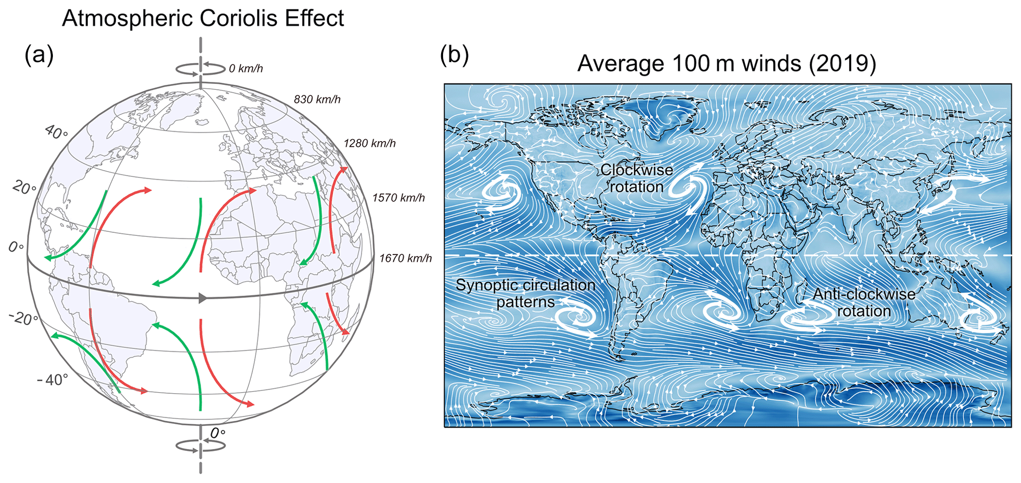
Figure 3 Illustration of the Coriolis effect on atmospheric circulation patterns. Panel (b) is produced using an average of the ERA5 100 m winds for 2019 at 12:00 UTC.

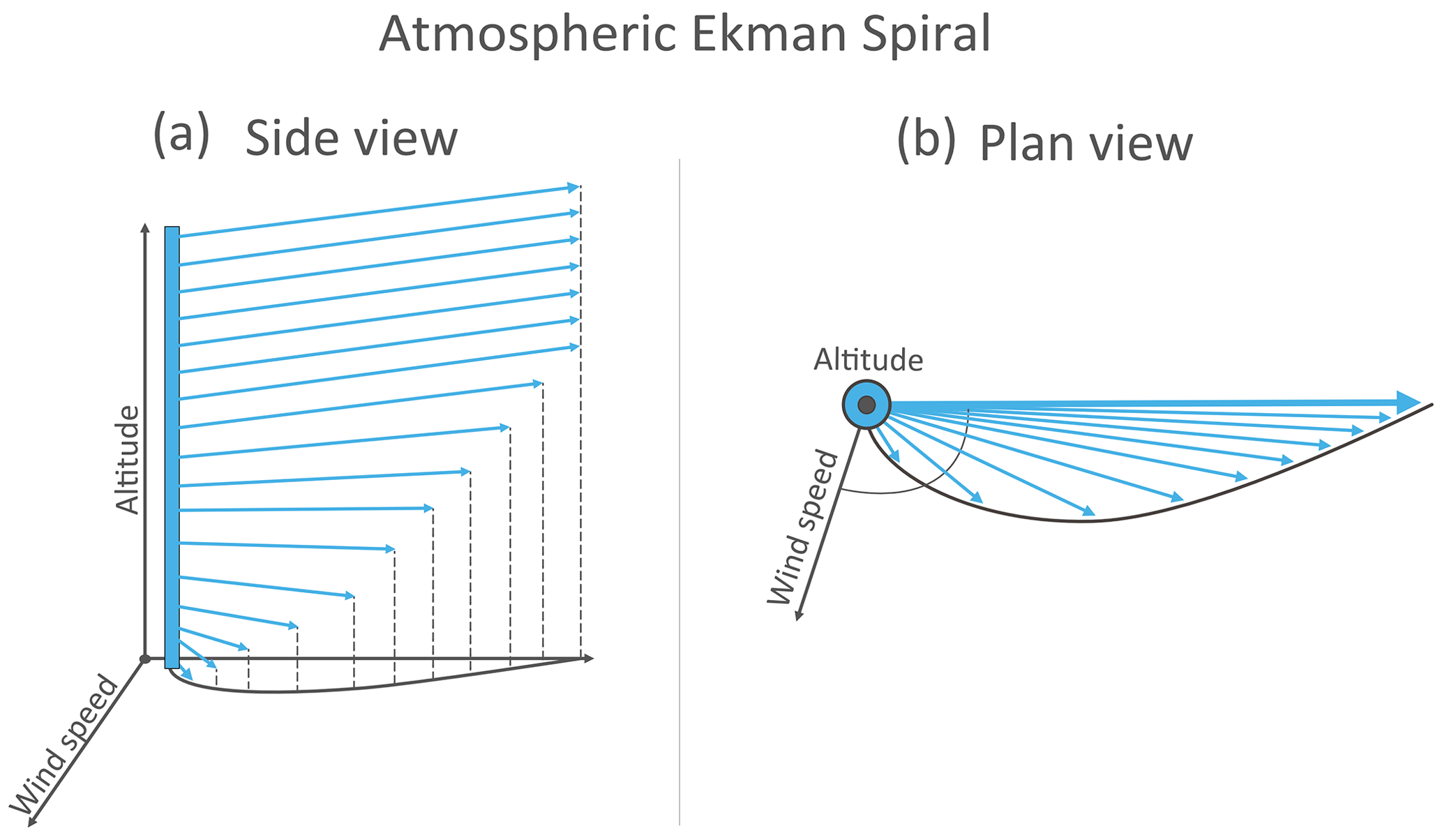
Figure 4 Schematic describing the process behind an Ekman spiral from the (a) side and (b) plan views. This diagram shows the spiral for the Southern Hemisphere.

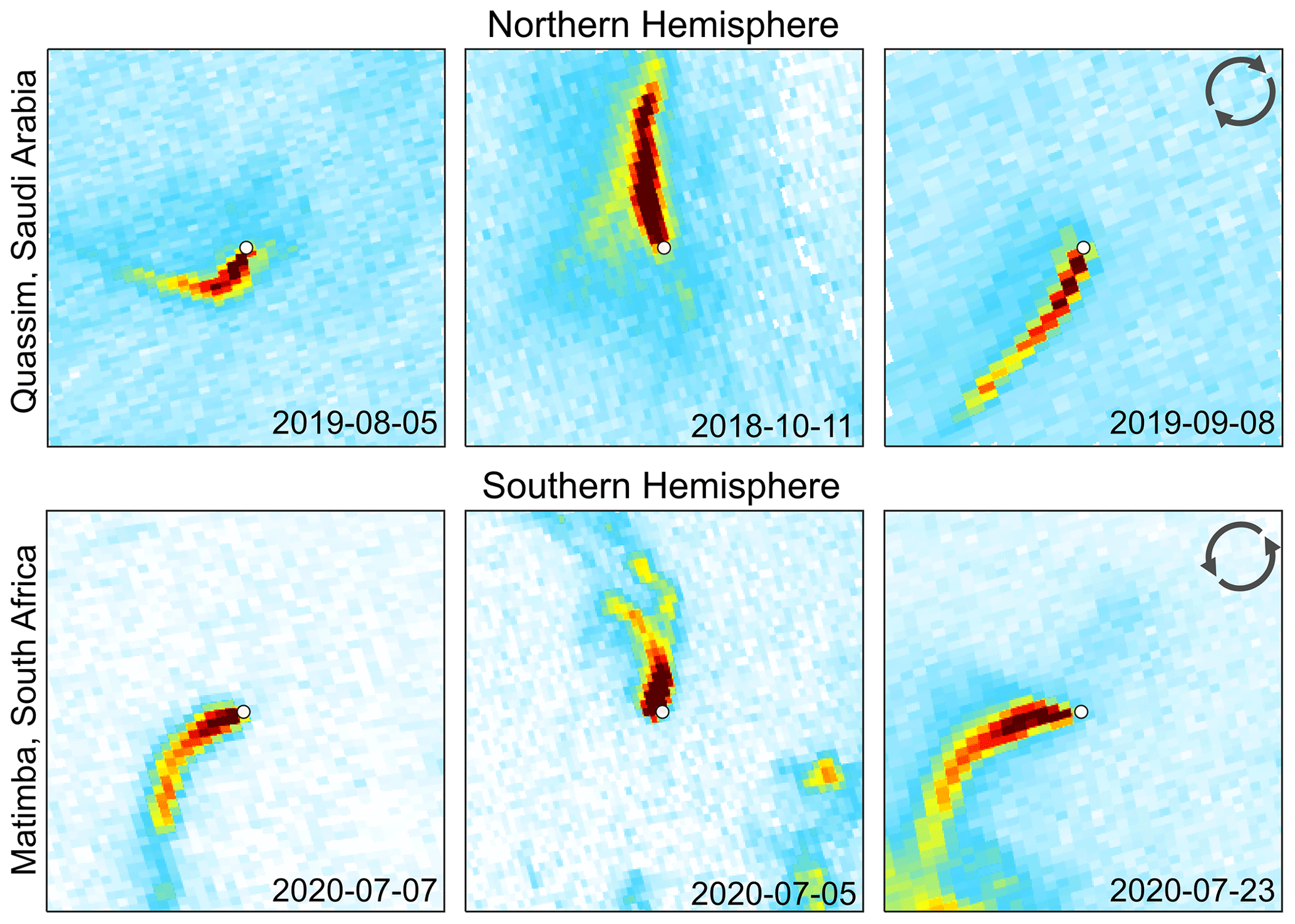
Figure 5 Example of the Coriolis influence on NO₂ emission plumes from daily TROPOMI NO₂ observations above Quassim (Saudi Arabia) and Matimba (South Africa). Power stations are shown as the central white dot in each observation.

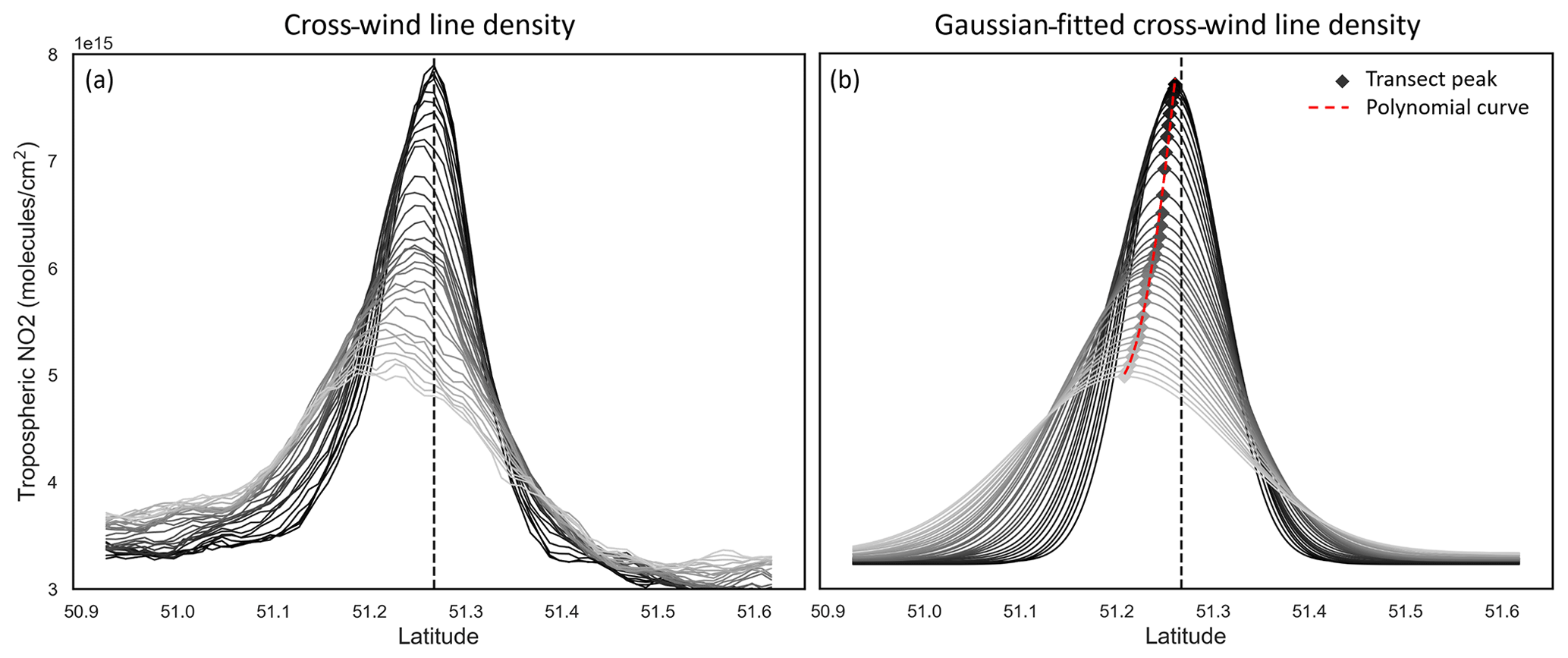
Figure 6 Across-wind line density profiles (a) and Gaussian-fitted line density profiles (b) taken at regular 1 km transects for the wind-rotated average of Belchatow power station in Poland. The transect at the origin is given by the black line, with the gradient getting lighter as the distance from the origin increases. Produced using data from May 2018 to November 2021.

$$\begin{array}{}\text{(2)}& \begin{array}{rl}& F_x=\mathrm{2}\cdot \mathrm{\Omega }\cdot \sin \left(\mathit{\varphi }\right)\cdot v\\ & F_y=\mathrm{2}\cdot \mathrm{\Omega }\cdot \sin \left(\mathit{\varphi }\right)\cdot u\end{array}\end{array}$$

In the above expression, F is the horizontal components of the Coriolis force, Ω is the Earth's rotation, ϕ is latitude, and v and u are the horizontal components of the wind. NO₂ emissions from large industrial sources can extend tens of kilometres and can rise quickly due to their thermal buoyancy. Emission plumes do not move independently nor freely within the atmosphere but instead follow the given wind field. This wind field is influenced in part by the Coriolis effect; thus, it follows that observed emission plumes of significant magnitude will be deflected due to the Coriolis effect as they move with the air mass. Furthermore, as the plume ascends due to its thermal buoyancy and the wind field's inherent vertical velocity, the plume will move to a degree with an Ekman spiral (Ekman, 1905; Åkerblom, 1908), which itself is a consequence of the Coriolis effect and is demonstrated in Fig. 4. The boundary layer can be considered in three parts (from lowest to highest): (1) the “laminar sublayer”, which only concerns the very near surface; the “Prandtl layer” (20–100 m), in which surface turbulence is fully developed but there is no influence from the Earth's rotation; and the “Ekman layer” (100–1000 m), in which movement is driven by the balance between pressure gradients, frictional effects, and the Coriolis force (Holton, 2004; Marshall and Plumb, 2016) and is strongly dependent on thermal stability (Sorbjan, 2003). At the surface, frictional forces bring the wind speed towards zero. The influence of these frictional forces decreases with height and along the pressure gradient, and so the wind speed increases with altitude towards the geostropic wind. As the Coriolis force is a function of wind speed, as shown in Eq. (2), and as wind speed increases with altitude, winds at the surface are oriented at an angle to winds further up the vertical column until laminar flow is reached near the boundary layer, creating the Ekman spiral. Whilst a mathematically pure Ekman spiral is rarely observed in a real atmosphere, the Ekman layer does impart a degree of curvature within the boundary layer relative to the geostrophic wind, increasing in angle with depth (Holton, 2004). The plumes in question are thermally buoyant and are inserted from a 100–300 m chimney into the Ekman layer, where their curvature will be modified both by the Coriolis force horizontally and via the Ekman spiral as it travels vertically with the air mass. This introduces variability in the magnitude of deflection, as magnitude is dependent on altitude, and the altitude that the plume reaches is dependent on its exit velocity, temperature, and, most importantly, the meteorology, which will vary day to day. Plume curvature becomes an issue when observations are rotated into an upwind–downwind aggregate to derive emissions, as the averaged plume may exhibit strong curvature and be unevenly distributed to one side of the common downwind axis. This deflection can be seen in some previous wind-rotated averages in other works, such as Fig. 4 of Hakkarainen et al. (2021), although its presence is not discussed. Examples of strong emission plume curvature from two of our investigated sites are given in Fig. 5. Whilst this study focuses on aggregate observations and the implications of curvature on emission estimates, further investigation into the conditions that produce extreme curvature in daily observations is required. High-curvature cases like these are likely a combination of high wind speed as well as favourable conditions for plume rise, where the Coriolis force and the Ekman spiral both contribute to the observed curvature. Meteorological dispersion modelling would be required to explore this, which is beyond the scope or aims of this study. Effects such as Coriolis curvature and Coriolis-induced Ekman spirals are just two of the many influences on the movement of the atmosphere, and various micro-, meso-, and synoptic-scale processes all contribute with variable intensity. Consequently, wind fields are not always dominated by the Coriolis effect, and they can circulate in the opposing direction to the Coriolis force or not at all; thus, not every observation will show the same magnitude or “expected” direction of curvature for that hemisphere. However, on average, we expect emission plumes to curve in favour of the direction of the Coriolis force for that hemisphere.

2.6 Curvature fitting

In order to evaluate the curvature of the wind-rotated plume, a “spine” was fitted to the aggregate. Firstly, the across-wind line density for 1 km transects perpendicular to the downwind axis were taken, as shown in Fig. 6a. These profiles show a characteristic normal distribution, with the maxima transect located near the origin. The origin here corresponds to the west–east “downwind” axis used for the wind-rotated aggregate. At greater distances downwind, the maximum of each transect laterally deviates with increasing distance from the origin, due to the curvature introduced by the Coriolis effect. These profiles contain a degree of noise; thus, a Gaussian smoothing procedure is applied, as displayed in Fig. 5b. This allows for the maxima of each transect to be more readily identified above the per-pixel variability. These peaks are then fitted with a second-order polynomial to identify the spine of the plume and the degree of deviation from the origin (shown in Fig. 6b as a dashed red line). This spine is shown in later figures as a dashed black line.

2.7 Emission estimation via an exponentially modified Gaussian (EMG)

To derive emissions from a wind-rotated aggregate, an exponentially modified Gaussian (EMG) (Beirle et al., 2011; de Foy et al., 2015; Fioletov et al., 2015; Goldberg et al., 2019) is fitted to the integral of the across-wind line densities in Fig. 6, the form of which is given in Eq. (3).

$$\begin{array}{}\text{(3)}& \begin{array}{rl}{\mathrm{NO}}_{\mathrm{2}}\mathrm{line}\mathrm{density}& =\mathit{\alpha }\left[{\displaystyle \frac{\mathrm{1}}{x_o}}\exp \left({\displaystyle \frac{\mathit{\mu }}{x_o}}+{\displaystyle \frac{{\mathit{\sigma }}^{\mathrm{2}}}{\mathrm{2}{x}_o^{\mathrm{2}}}}-{\displaystyle \frac{x}{x_o}}\right)\right.\\ & \left.\mathrm{\Phi }\left({\displaystyle \frac{x-\mathit{\mu }}{\mathit{\sigma }}}-{\displaystyle \frac{\mathit{\sigma }}{x_o}}\right)\right]+\mathit{\beta }\end{array}\end{array}$$

$$\begin{array}{}\text{(4)}& {\mathrm{NO}}_{\mathrm{x}}\mathrm{emissions}=\mathrm{1.33}\left({\displaystyle \frac{\mathit{\alpha }}{{\mathit{\tau }}_{\mathrm{eff}}}}\right),\text{where}{\mathit{\tau }}_{\mathrm{eff}}={\displaystyle \frac{x_o}{\mathit{\omega }}}.\end{array}$$

Here, α is the total number of NO₂ molecules minus the background, β. x_o is the e-folding distance downwind of the source, μ is the displacement of the apparent source relative to the assumed source centre, σ is the standard deviation of the Gaussian function, and Φ is the cumulative distribution function. Using a non-linear iterative least squares fitting approach, α, x_o, σ, μ, and β are determined. This process is illustrated in Fig. 7. From these fitted parameters, we can then calculate an effective lifetime (τ_eff) using the mean wind speed (w). Equation (4) is then used to calculate NO_x from the TROPOMI-derived NO₂, using τ_eff and a scaling factor of 1.33 to convert NO₂ to NO_x. This scaling factor describes the typical ${\mathrm{NO}}_{\mathrm{2}}/\mathrm{NO}$ ratio under polluted conditions at noon (Seinfeld and Pandis, 2016).

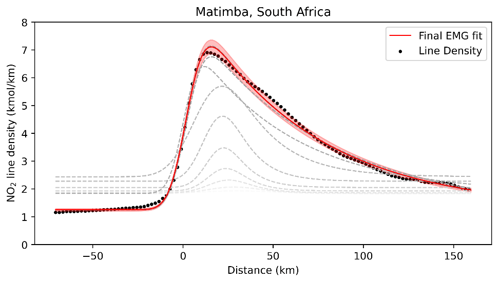
Figure 7 Demonstration of the Curvefit process of fitting the exponentially modified Gaussian (EMG) to the NO₂ line density. The figure was produced using wind-rotated NO₂ from Matimba power station for the period from May 2018 to November 2021. The red line shows the final EMG fit, and the grey lines illustrate the iterative fitting procedure (changing from light grey to black as they converge to the final EMG fit).

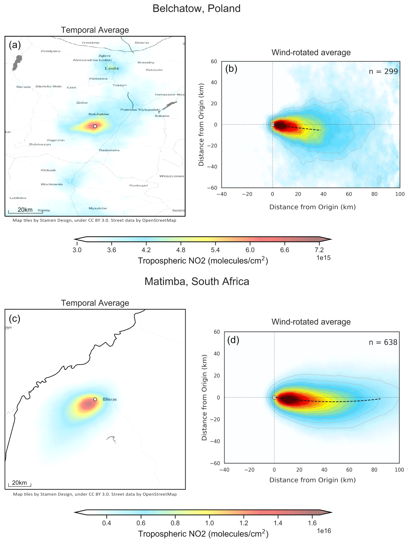
Figure 8 Unrotated and wind-rotated average tropospheric NO₂ columns from TROPOMI, using data from May 2018 to December 2021, for (a–b) Belchatow power station in Poland and (c–d) Matimba power station in South Africa. Map tiles were created by Stamen Design (CC BY 3.0). Street data were obtained from OpenStreetMap (ODbL).

3 Results and discussion

3.1 Wind rotation aggregates of selected sites

Figure 8 shows both the unrotated and wind-rotated aggregates for Belchatow power station in Poland (Fig. 8a, b) and Matimba power station in South Africa (Fig. 8c, d), as examples of a respective Northern Hemisphere and Southern Hemisphere sites. The dashed black line shows the spine of the plume, and the value of n shows the number of observations included in the aggregate. Both sites are strong emitters that are well isolated from other sources, and the surrounding area consists of relatively simple topography. Both of these sites show strong curvature in their wind-rotated aggregates, and, whilst the plume's structure is successfully preserved, there is a clear distinguishable curvature in favour of the Coriolis force direction. As these two example sites are not coastal and are in regions with simple topography, there are minimal micro- or meso-scale processes influencing the wind field; thus, the effect of the Coriolis force is easily identified, as it more frequently prevails over other influences. The remaining sites are shown the Appendix (Figs. A1, A2, A3), grouped by their hemisphere. Of the 16 sites investigated, 9 showed the expected curvature for the hemisphere they reside in (although the magnitude of the this varied), 5 showed no or negligible curvature, and 2 showed opposing or unusual curvature. These latter two sites are located in areas with steep and highly variable topography that may “steer” plumes locally, and such “steering” may dominate over larger-scale Coriolis curvature. A good example of this is given in Fig. 9: the Jorge Lacerda power station is located in Brazil at a latitude of −28.45 in the Southern Hemisphere, yet we observe clockwise, Northern Hemisphere curvature. This can be explained by the topographical surroundings of Jorge Lacerda, as the power station sits between the South Atlantic and the Serra do Mar coastal mountain range, where there is an abrupt >1200 m increase in altitude over a short distance. Onshore synoptic-scale winds and sea breeze penetrate inland and are “steered” by the topography. These local effects, over tens of kilometres, dominate over larger synoptic weather patterns and, therefore, outweigh the influence of the Coriolis effect, leading to this unexpected display of Northern Hemisphere curvature.

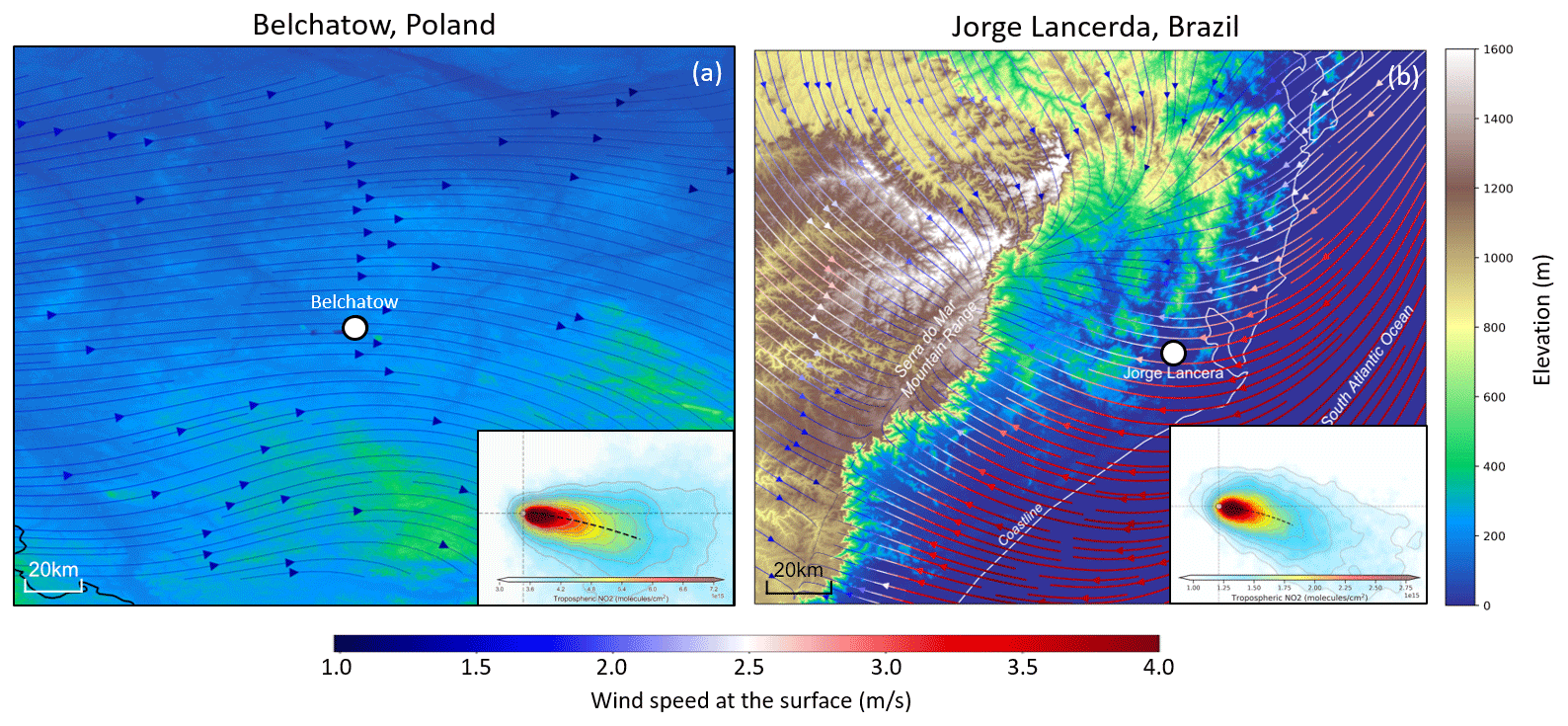
Figure 9 (a) Average 2018 surface wind fields from the ERA5 reanalysis, including topography from the Copernicus GLO-30 digital elevation model for (a) Belchatow in Poland and (b) Jorge Lacerda in Brazil. The insets in panels (a) and (b) show the wind-rotated tropospheric NO₂ columns from TROPOMI, using data from May 2018 to December 2021.

3.2 Impact of the selected wind level on the quality of the aggregate

To investigate the influence of the chosen wind field on the final aggregate and emission value, emissions were derived for Matimba using wind fields corresponding to the following pressure levels: 900 hPa (∼ 100 m), 875 hPa (∼ 250 m), 850 hPa (∼ 450 m), 825 hPa (∼ 700 m), 800 hPa (∼ 1000 m), and an average of all six levels. As seen in Fig. 10, the plume migrates anticlockwise with increasing altitude, e.g. the plume spine is below the aggregate x axis at 900 hPa (∼ 100 m) but above it at 800 hPa (∼ 1000 m). Due to the Ekman spiral, winds near the surface are oriented clockwise (for the Southern Hemisphere, as used in this example) compared with winds at higher altitude; thus, rotational alignment using winds at lower altitude results in a clockwise deviation compared with alignment using winds at higher altitude, which is to be expected. The initial stages (first 10 km downwind) of each plume align with the aggregated x axis and are laterally symmetric around it. This confirms that rotations based on the wind vector near the source produce well-aligned and symmetric aggregate plumes in the near field; however, the Coriolis curvature becomes distinguishable from the initial alignment at greater distances, and it is increasingly deviated and asymmetric relative to the common axis as the plume progresses downwind. Aggregates using winds at 900–850 hPa are very similar, with 825–800 hPa showing better initial alignment with the axis of aggregation, within the first 10 km. This initial agreement may be due to the wind direction at these levels being the most representative or due to an inherent bias in the ERA5 model, as there may be small but consistent differences between the wind at the site and the coarse 0.25^∘ × 0.25^∘ modelled fields. All exhibit comparably strong curvature, which shows that curvature is not an artefact of the wind product but rather an inherent feature of the observations. Furthermore, wind speed increases with altitude, and, as wind speed factors into the emission calculation, it is important that representative wind fields are used, rather than selecting purely by the field that yields the best initial alignment. For the purposes of this study, the average wind field is used, as it results in good plume alignment in most cases whilst also reasonably describing the wind speeds experienced as the plume travels downwind both vertically and horizontally from the source. Although the 800 hPa aggregate has the best initial alignment, these higher wind speeds would not be experienced by the plume for the majority of its lifetime and would lead to an overestimate in the emission, as demonstrated by Fig. A4. There must be a trade-off between the geometric alignment of the aggregated plumes and ensuring that the wind field reasonably describes the wind speeds experienced.

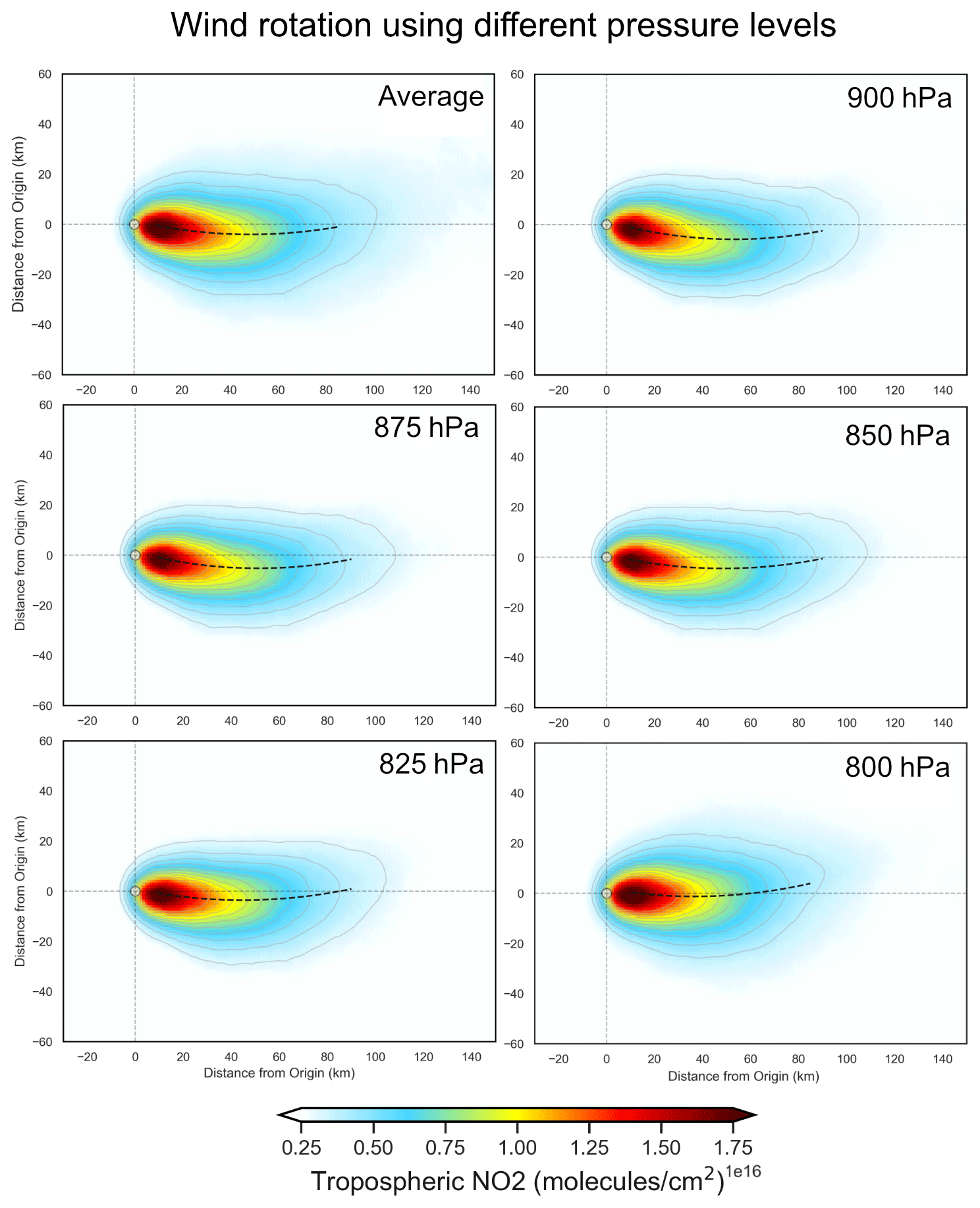
Figure 10 Demonstration of the difference in aggregate when using wind products from different pressure levels, using data from Matimba power station for May 2018–November 2021.

3.3 Impact of the Coriolis curvature on the emission estimates

From the wind-rotated aggregate, the typical next step is to take the integral of evenly spaced (1 km) across-wind (±30 km) segments perpendicular to the x axis, as shown in Fig. 11a.

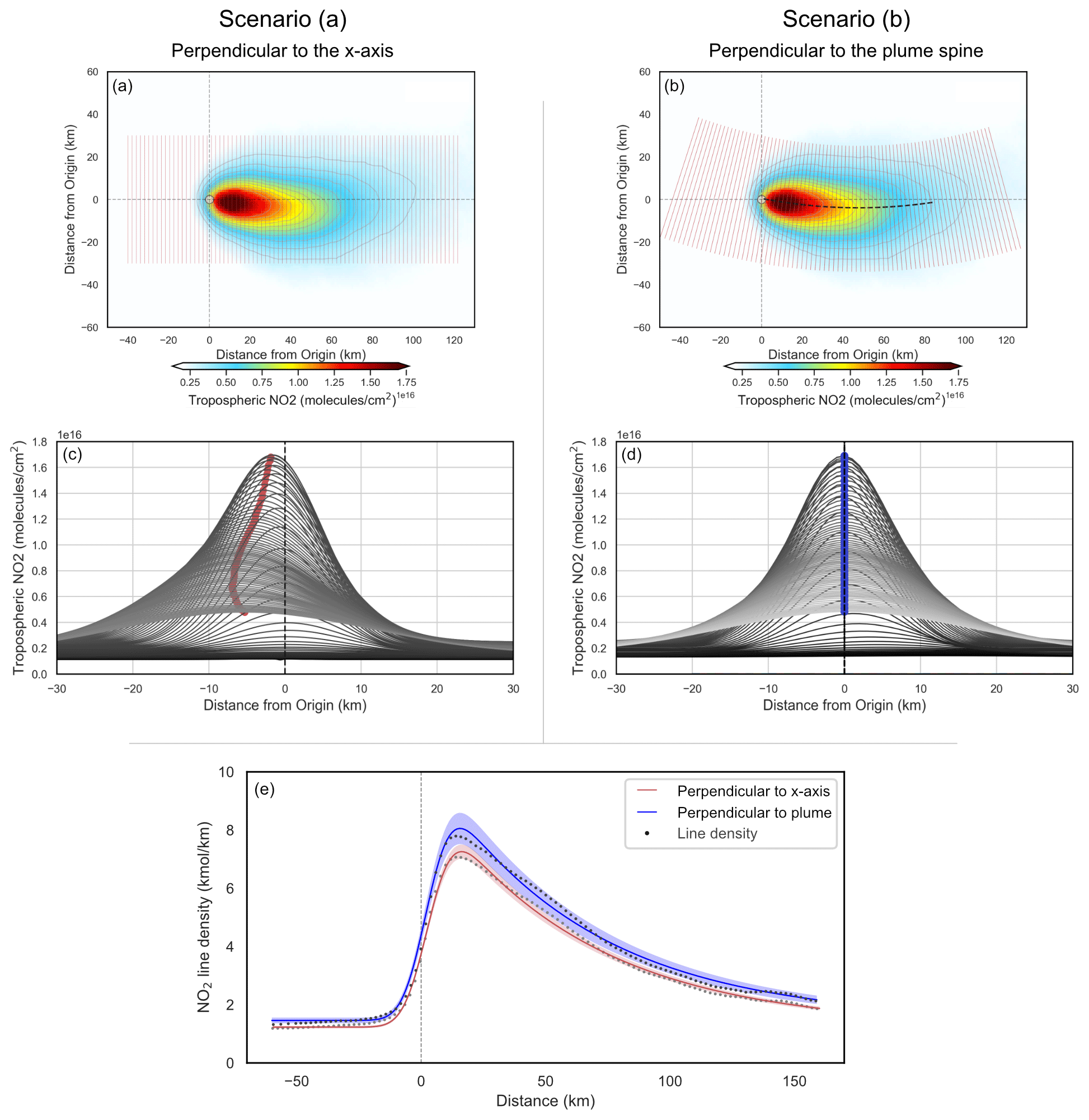
Figure 11 Demonstration of the impact that the Coriolis effect has on the resulting emission estimate. Panels (a) and (c) show the results using cross sections perpendicular to the x axis, whereas panels (b) and (d) show cross sections perpendicular to the plume of the spine. Panel (e) shows the EMG fit for each scenario, with the shaded region showing the quality of each fit.

This approach assumes that the wind-rotated plume is distributed evenly either side of the common axis. Occasionally this assumption holds, as the curvature is often minor/negligible and, thus, emission estimates are marginally impacted. However, as evident from sources such as Matimba, this is not always the case, and the plume can deviate considerably from the x axis due to the plume’s inherent curvature. Using the EMG emission estimation method discussed in Sect. 2.7, we calculated NO_x emissions for Matimba under two scenarios: (a) using cross-wind segments perpendicular to the common downwind axis and (b) using cross-wind segments perpendicular to the curved spine of the plume. Scenario (b) aims to counteract the influence of the plume’s geometry on the emission estimate by re-centring the integral along the curved spine of the plume. Uncertainties are determined using a bootstrapping approach, whereby observations are randomly selected, with replacement, to be included in the aggregate. Each scene has both measurement and numerical error; thus, by assuming these errors are randomly distributed, the random selection and replacement of scenes in the bootstrapping algorithm allow for the estimation of the impact that all of these errors have on the emission estimate (de Foy et al., 2015, 2014). Uncertainty introduced by the selection of the wind field is evaluated through sensitivity tests, in which emissions are calculated using each pressure level, as shown in Fig. A4. This approach does not account for uncertainty introduced due to the clear-sky bias, caused by only using cloud-free observations. Figure 12 shows annual NO_x emission estimates for Matimba power station using the following four scenarios: (1) a similar study of Matimba using TROPOMI NO₂ and EMG before S5P-PAL released (Hakkarainen et al., 2021); (2) scenario (a); (3) scenario (b); and, finally, (4) reported values from the site operator, Eskom, derived from continuous emission monitoring system (CEMS) data (https://www.eskom.co.za/dataportal/emissions/ael/matimba-c2/, last access: 1 July 2022). The reported emissions are not provided with an uncertainty; therefore, conclusive statements about the accuracy of the TROPOMI-based estimate are not possible. The use of S5P-PAL explains the increase in emissions between Hakkarainen et al. (2021) and scenario (a), as S5P-PAL can lead to a 10 %–15 % increase in tropospheric columns for polluted cloud-free scenes (Eskes et al., 2019). This translated to a 5 %–10 % increase in the emission estimate for Matimba power station. Between scenarios (a) and (b) there is a substantive 9.1 %±1.92 % increase in emissions annually on average, for the years 2018–2021, when the curved geometry of the wind-rotated plume is taken into account. Scenario (b) yields an emission value closer to the reported value, and its uncertainty is within range of the reported emissions for 3 out of the 4 years investigated. This strongly suggests that an improved satellite-derived emission estimate can be achieved by considering the curvature of the wind-rotated aggregate. This approach is not constrained to the Coriolis effect, as any consistent misalignment of the aggregated plume, such as the topographic deviation seen at Jorge Lacerda, could be accounted for when calculating emissions by following the method discussed here. This approach is rather generalised and could be easily applied autonomously to a given source.

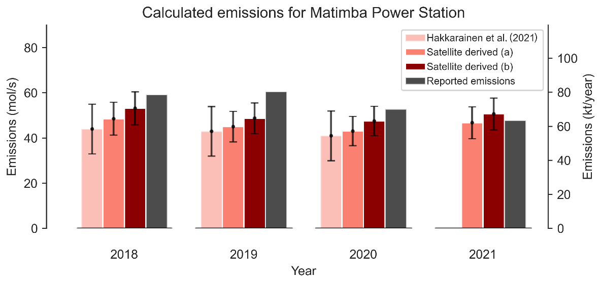
Figure 12 Comparison of emission estimates from TROPOMI NO_x using different applications of the EMG method, values obtained by Hakkarainen et al. (2021) for the same site, and emissions reported from estimates by the operator, Eskom (https://www.eskom.co.za/dataportal/emissions/ael/matimba-c2/, last access: 1 July 2022).

We suggest that the spine fitting and along-spine integration steps should be incorporated into a regulatory wind rotation aggregation approach, in order to minimise the influence of plume curvature on the emission estimate.

4 Conclusions

This study demonstrates the Coriolis effect’s varying influence over the trajectory of point source emission plumes observed by TROPOMI. Moreover, it shows how strong curvature can lead to substantive underestimations in the emission estimate if it is not accounted for. Of the 16 locations investigated, 9 showed the expected curvature for the hemisphere that they reside in (although with varying magnitude), 5 showed no or negligible curvature, and 2 showed opposing or unusual curvature. The sites that showed conflicting curvature are all within regions with complex terrain where airflows are steered by local topography in ways that dominate over larger-scale influences such as the Coriolis effect. Emissions of NO_x were estimated for Matimba power station in South Africa, which was chosen due to its strong curvature and good data coverage. Conducting the emission calculation in a way that accounted for the inherent curvature of the plume resulted in an average ∼ 9 % increase in yearly emitted NO_x over the regular approach and was more comparable to and within the uncertainty range of the emission value reported by the operator. As demonstrated, the wind-rotated aggregate of a source is not always aligned and distributed along the common downwind axis; therefore, site-specific considerations need to be included. This study formally identifies, for the first time, Coriolis curvature in the satellite record and suggests how it can be accounted for during emission analysis of high-curvature cases, such as Matimba power station. Considerable work remains with respect to understanding the conditions that drive the more extreme curvature cases, such as those shown in Fig. 5. The dynamics of the atmosphere have been well researched, but the behaviour of these variable emission plumes released from height at considerable temperatures has received less attention, especially with respect to characterising their trajectory and curvature. Hence, a greater understanding of the combined and variable contributions of horizontal Coriolis curvature with the additional curvature induced by the Ekman spiral, which is essential for correctly interpreting observations of these plumes in the satellite record, is required. For satellite evidence to be used by regulators and operators, there needs to be a standardised data processing routine in place for emission calculation and uncertainty analysis, as there is with air quality modelling, so that satellite observations can be used to generate consistent and auditable evidence of emissions for regulatory purposes. The rapid development of satellite instruments over the next decade will offer a unique opportunity for air quality regulators and industrial operators to begin to monitor emission performance remotely and persistently; therefore, a greater understanding of the role atmospheric dynamics has in satellite-derived emission estimates is vital.

Appendix A

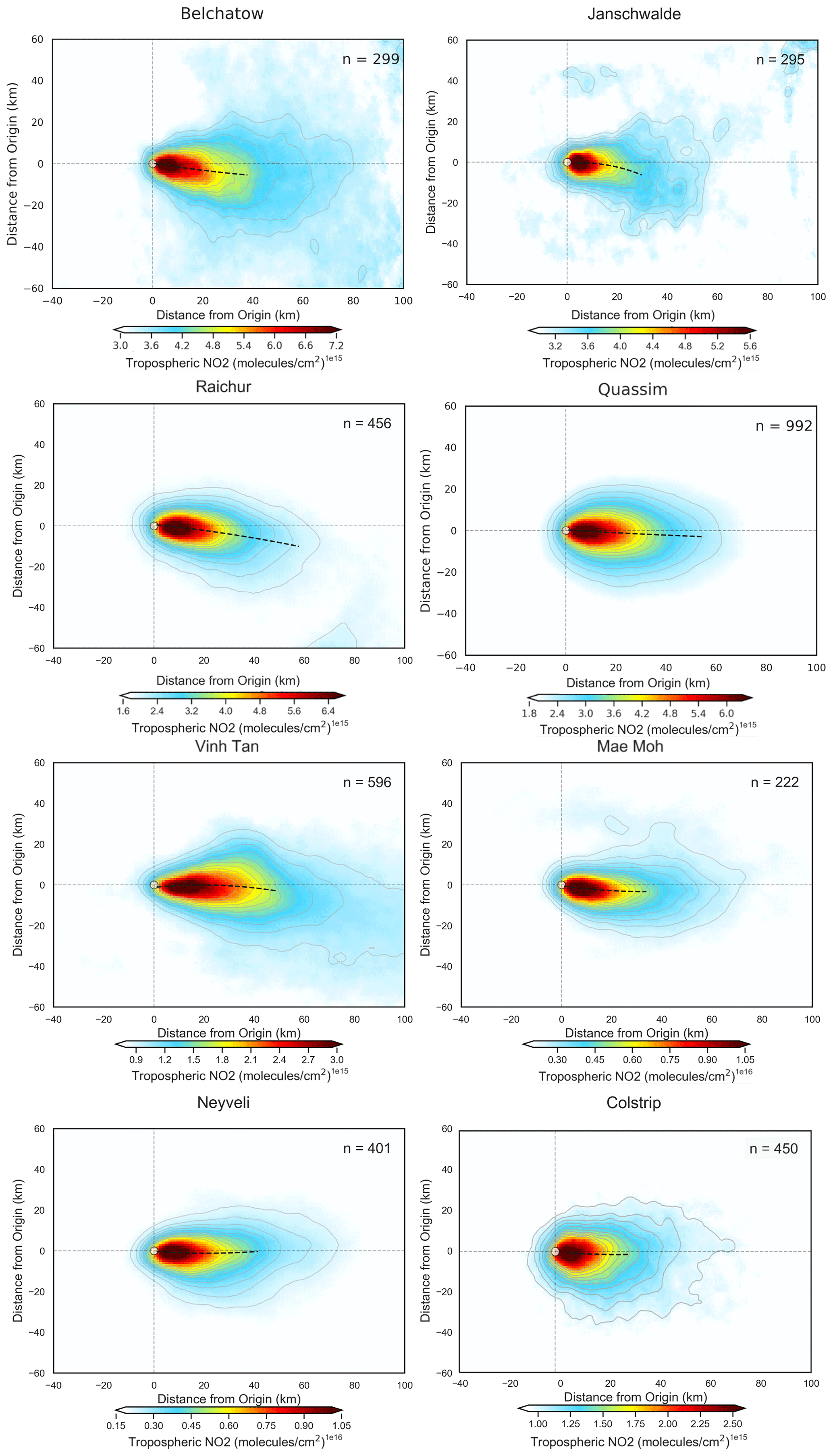
Figure A1 Wind-rotated aggregates of all Northern Hemisphere sites, with the plume spine signified by the dashed black line.

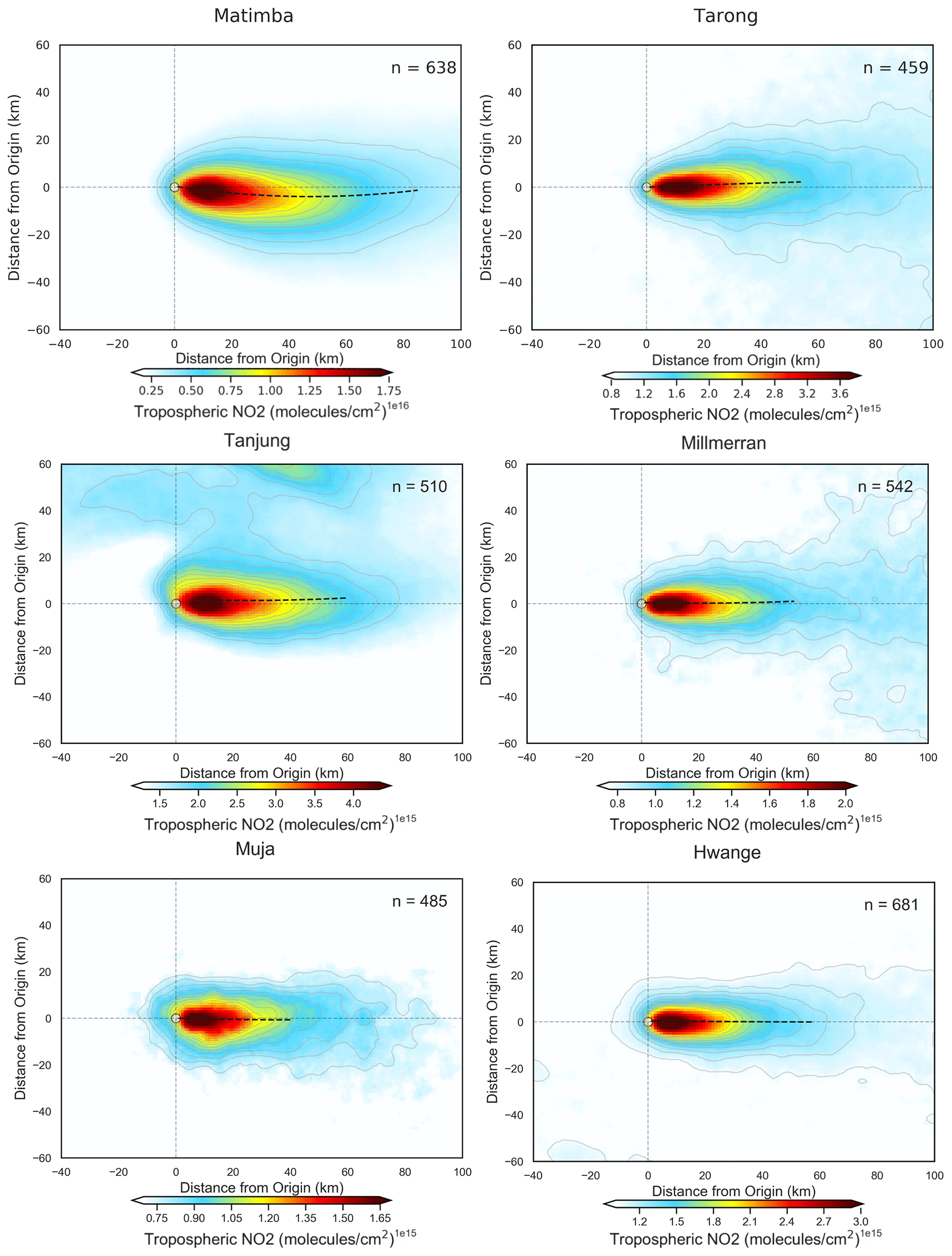
Figure A2 Wind-rotated aggregates of all Southern Hemisphere sites, with the plume spine signified by the dashed black line.

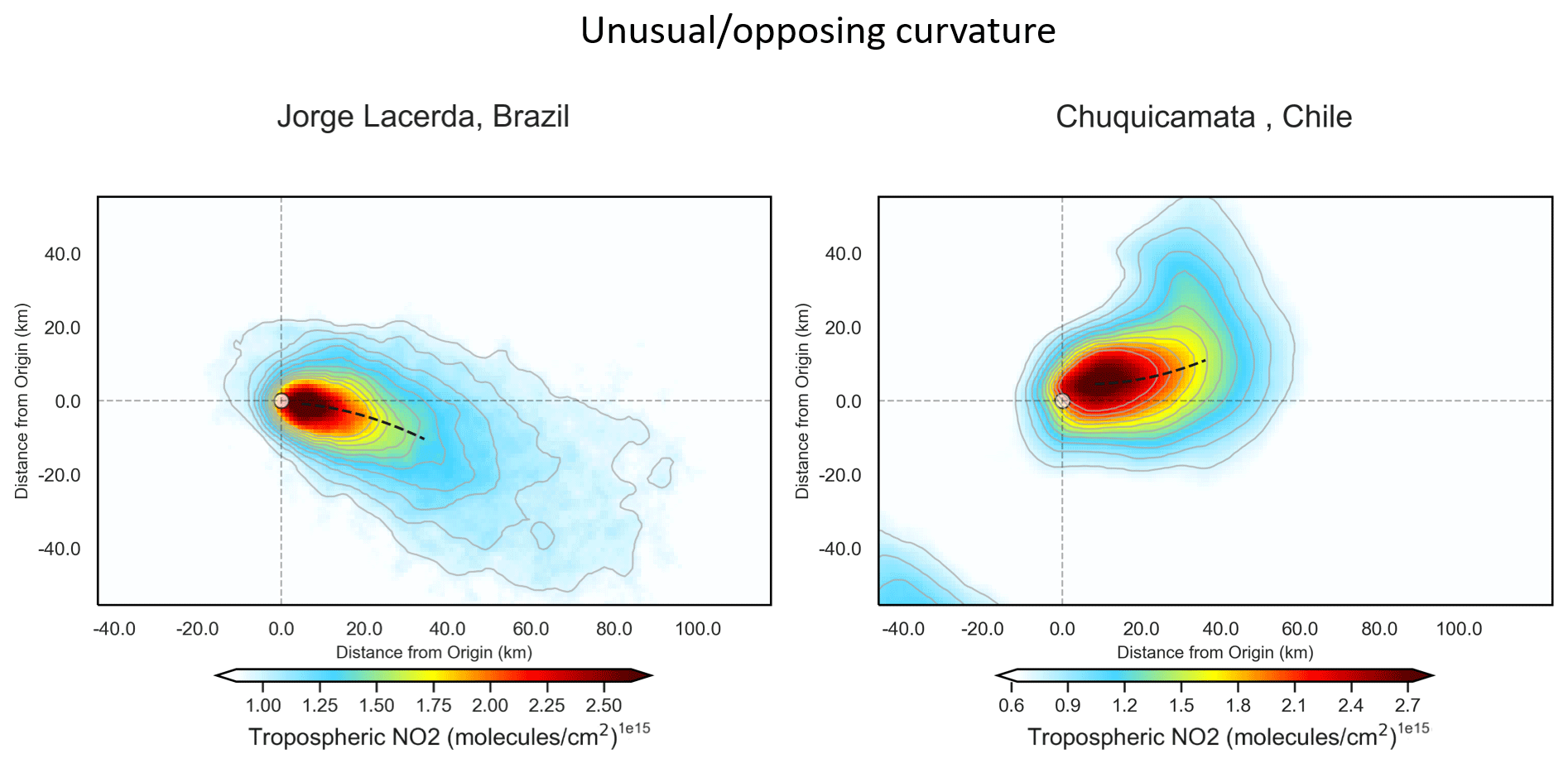
Figure A3 Wind-rotated aggregates of the non-conforming sites, with the plume spine signified by the dashed black line.

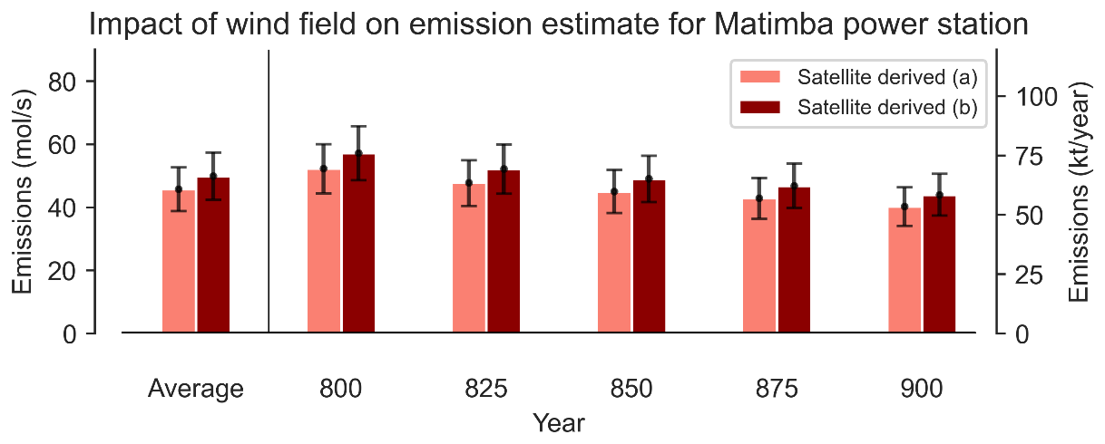
Figure A4 Demonstration of the influence that the chosen wind product has on the final emission estimate using data for the entire 2018–2021 period from Matimba power station.