the Creative Commons Attribution 4.0 License.
the Creative Commons Attribution 4.0 License.
 | 13 Apr 2023
Aerosol deposition to the boreal forest in the vicinity of the Alberta Oil Sands
Timothy Jiang
Paul A. Makar
Ralf M. Staebler
Michael Wheeler
Measurements of size-resolved aerosol concentration and fluxes were made in a forest in the Athabasca Oil Sands Region (AOSR) of Alberta, Canada, in August 2021 with the aim of investigating (a) particle size distributions from different sources, (b) size-resolved particle deposition velocities, and (c) the rate of vertical mixing in the canopy. Particle size distributions were attributed to different sources determined by wind direction. Air mixed with smokestack plumes from oil sands processing facilities had higher number concentrations with peak number at diameters near 70 nm. Aerosols from the direction of open-pit mine faces showed number concentration peaks near 150 nm and volume distribution peaks near 250 nm (with secondary peaks near 600 nm). Size-resolved deposition fluxes were calculated which show good agreement with previous measurements and a recent parameterization. There is a minimum deposition velocity of vd=0.02 cm s−1 for particles of 80 nm diameter; however, there is a large amount of variation in the measurements, and this value is not significantly different from zero in the 68 % confidence interval. Finally, gradient measurements of aerosol particles (with diameters <1 µm) demonstrated nighttime decoupling of air within and above the forest canopy, with median lag times at night of up to 40 min and lag times between 2 and 5 min during the day. Aerosol mass fluxes (diameters <1 µm) determined using flux–gradient methods (with different diffusion parameterizations) underestimate the flux magnitude relative to eddy covariance flux measurements when averaged over the nearly 1-month measurement period. However, there is significant uncertainty in the averages determined using the flux–gradient method.
- Article
(2096 KB) - Full-text XML
- BibTeX
- EndNote


Atmospheric aerosols have a strong influence on climate, affecting the radiation budget (both directly and indirectly) through radiative reflection, absorption, and influence on cloud formation. The net radiative effect is a large source of uncertainty in climate models (Boucher et al., 2013). Human exposure to particulate matter is linked to respiratory and cardiovascular disease and increased mortality, with some studies showing health effects even at very low concentration exposures (Kappos et al., 2004). Forests comprise 9 % of the land surface on Earth (Adams, 2012) and 40 % of the land surface of Canada (NRCan, 2021), and they are a net sink of aerosols due to dry deposition. Aerosol deposition to forests also affects the health and growth of the forest (Matsuda, 2017). Hence, modeling deposition to forests is key to correctly modeling atmospheric aerosol concentrations.
The Athabasca Oil Sands Region (AOSR) in Alberta, Canada, is the third-largest oil deposit in the world. The activities associated with mining and bitumen processing in the region generate pollutants, greenhouse gases, and aerosols. The aerosols include sulfates, black carbon, primary organic aerosol (POA), dust, and secondary organic aerosol (SOA) (Liggio et al., 2016) with SOA formation rates comparable to large North American cities. Aerosols thus originate in both direct emissions (primary) and in situ reactions of gases (secondary).
Several aircraft-based studies have characterized the composition and size of the oil sands aerosols in the region (Howell et al., 2014; Baibakov et al., 2021; Liggio et al., 2016) by flying through elevated plumes downwind of mines and upgrading facilities. Howell et al. (2014) characterized the aerosols as a mix of freshly nucleated sulfates and nitrates, possible fly ash, and dust from dirt roads and mining operations, while Baibakov et al. (2021) found that the plumes were associated with elevated concentrations of sulfates and ammonium. All three studies demonstrated the formation of organic aerosol within tens of kilometers of the sources, and Liggio et al. (2016) demonstrated that SOA formation rates are comparable to megacities such as Mexico City or Paris.
Surface loss of aerosols through dry deposition is primarily dependent on aerosol size and vegetation type. Extensive reviews of dry deposition of aerosols can be found in Hicks et al. (2016), Saylor et al. (2019), Farmer et al. (2021), and Emerson et al. (2020). The primary mechanism for the deposition of small particles <100 nm in diameter is Brownian diffusion, which is more effective for smaller particles. The primary mechanism for the deposition of large particles >300 nm in diameter is impaction and interception due to inertia. There is an intermediate size of particles for which both mechanisms are less effective, leading to the local minimum of deposition velocity of aerosols with respect to particle diameter, which is referred to in Hicks et al. (2016) as a “well” in deposition velocity of aerosols as a function of particle size. Emerson et al. (2020) demonstrated that previous parameterizations overestimate deposition for particles with diameters less than 500 nm and underestimate deposition for particles with diameters more than 2 µm. The overestimation can be as large as an order of magnitude.
The minimum in deposition velocity has been observed in a coniferous forest in southern Finland by Mammarella et al. (2011); however, these deposition velocities were not determined using size-resolved eddy covariance measurements. Instead, flux measurements were made using total number concentrations for particle diameters between 10 nm and 1 µm, and then the size dependence was inferred using a particle deposition model. Using this methodology, the Mammarella et al. (2011) study suggests a local minima of aerosol deposition velocity at particle diameters of 90 and 150 nm. The location of the minimum well was recently demonstrated by size-resolved eddy covariance aerosol flux measurements over a ponderosa pine forest by Emerson et al. (2020), who proposed a modification to the widely used Zhang et al. (2001) parameterization. Both the Emerson et al. (2020) and Zhang et al. (2001) parameterizations have a single minimum value at 0.01 to 100 µm range. The revised (Emerson et al., 2020) parameterization locates the minimum deposition velocity near 70 nm in diameter (closer to the measured values) compared to the minimum located near 2 µm in diameter predicted by the Zhang et al. (2001) model.
The presence of the crown of a forest canopy leads to frequent decoupling between the sub-canopy space and the air above the canopy. Only occasionally (an average of 4 h d−1) does the sub-canopy air exchange energy and matter with the air above the canopy (Thomas and Foken, 2007), and mixing often does not occur for several hours at a time through the night. The canopy is usually decoupled during calm conditions. Decoupling means that fluxes in and out of forests do not happen continuously but are discrete events (Foken, 2008). This is typically accounted for in models which include deposition by modifying the diffusion coefficient based on stability (e.g., Makar et al., 2017).
While forests are predominantly a sink for aerosols, forests can often be a source of aerosols to the atmosphere (e.g., Gordon et al., 2011; Pryor et al., 2008) either by adding biogenic mass to anthropogenic aerosols or by aggregation of organic matter. Furthermore, the influence of mixing and coupling on deposition is often significant where stagnant air in the understory can act as a blocking layer between the canopy top and the surface (Schilperoort et al., 2020).
In spite of the abundance of aerosol deposition studies in forests, there has not yet been such a study in the AOSR. The three primary goals of this study were to determine the sources of specific aerosol size distributions from oil sands operations at ground level, to determine the size-resolved deposition rate of anthropogenic source aerosols into forests, and to study the effect the forest has on the vertical mixing of aerosols. This paper is a companion paper to Gordon et al. (2022) and Zhang et al. (2023), which respectively investigate SO2 and ozone deposition at this site.
2.1 Site location and instrumentation
The York Athabasca Jack Pine (YAJP) tower was installed between July 2017 and October 2021 at 57.1225∘ N, 111.4264∘ W. This work describes results from three intensive field campaigns at the tower in 2017 (16 July–1 August), 2018 (4–18 June), and 2021 (3–26 August). Size-resolved aerosol measurements were made during all three campaigns, while eddy covariance fluxes were measured only in the 2021 campaign. The results presented here focus on the August 2021 study only due to the availability of eddy covariance fluxes during the latter period.
The tower was mounted within the forest and is accessed through an unimproved road originally used for reflection seismology. The closest paved road is the East Athabasca Highway, which is a private road with generally light traffic approximately 650 m to the south of the tower. The site is surrounded by at least 10 km of boreal forest in all directions (Fig. 1) with oil sands open-pit mining, tailings, and processing facilities beyond that, predominately in the 135–270 and 305–45∘ sectors. The Athabasca River valley runs west of the site in a varying north–south direction, which has an influence on local wind direction. The village of Fort McKay is approximately 15 km to the NW of the site, and the town of Fort McMurray is 40 km south. Additionally, the Hammerstone limestone aggregate quarry is located 10 km NW of the tower.
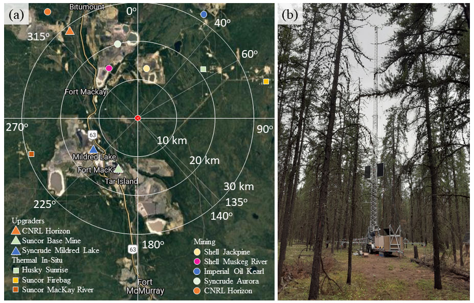
Figure 1(a) YAJP tower site location (red circle) and surrounding area with 10, 20, and 30 km radius circles. Radial directions shown (0, 40, 60, 135, 140, 225, and 315∘) are used to group observations by source. Image is © Google Maps (2020) with upgrader and mine locations added from Davidson and Spink (2018). (b) The tower and the surrounding jack pine forest.
The forest is mature jack pine (Pinus banksiana) and the ground is covered in reindeer moss (Cladonia spp.). The undergrowth in the area is limited to some sparsely distributed blueberry bushes. The ground is sandy and well drained. The forest's canopy height is approximated as 19 m (with the tallest trees in the area ranging from 16 to 21 m in height). The one-sided leaf area index (LAI) was measured as 1.17 (based on Gap Light Analyzer software, Frazer et al., 1999) with a stem density of approximately 320 trees per hectare. A generator was located 90 m from the tower at a wind angle of 50∘. During the entire 4-year duration of the project, less than 4 % of the wind was from the 40–60∘ direction.
The ultrahigh-sensitivity aerosol spectrometer (UHSAS, Droplet Measurement Technology Inc.) measures particle number concentration in 100 size ranges between 55 nm and 1 µm. Particles are sized and counted with 1054 nm laser light scattered onto two magnifiers (one for small particles and one for large ones) collected by photodiode. All references to diameter in this study refer to the optical diameter measured by the UHSAS. Cai et al. (2008) have demonstrated that there is more than 50 % loss for particles of size 55–60 nm and an underestimation of the size of particles on the smaller end of its range. We restrict our analysis to the 60 nm to 1 µm range. Size distributions were sampled at a 1 Hz frequency. The UHSAS was installed at the base of the tower and sampled from a height of 29 m through a 32 m length of ” inner-diameter static dissipative tubing. The measured flow rate of 15 L min−1 results in a residence (delay) time of 9 s. The instrument response time (with the 32 m tubing length) was determined in lab tests by measuring step changes in concentration and fitting the response to a sigmoid curve (Horst, 1997). This gave a response time of τ=0.9 s. Petroff et al. (2018) determined a response time of 0.28 s for the UHSAS alone, suggesting that approximately 0.6 s of our measured response time is due to dissipation in the tubing.
A 3D sonic anemometer (Type A, Applied Technology Inc.) was co-mounted with the UHSAS inlet at 29 m. The anemometer faced approximately south (169∘) and was mounted 0.7 m from the tower structure (which is an open triangular cross-section with 0.4 m sides). For the 2017 field study, a second anemometer was mounted at a height of 9 m within the canopy. The anemometers sampled at a frequency of 10 Hz.
Two particle counters (DustTrak DRX 8533, TSI) were mounted at ground level (2 m) and at a height of approximately 20 m. The DustTrak particle counters sample 2 min averages of total particle mass for an approximate range of 0.1 to 15 µm. These measurements are size-resolved into total mass for diameters less than 1 µm (PM1), 2.5 µm (PM2.5), 4 µm (PM4), and 10 µm (PM10). Here, we only used the PM1 (0.1 to 1 µm) size range. The instruments were set to auto-zero every 15 min. Yun et al. (2015) found that the DustTraks require a correction factor of 0.29 for PM2.5. The DustTrak measurements were concurrent with the UHSAS particle concentration sampled at 29 m. This allowed a comparison of PM1 at heights of 20 m (DustTrak) and 29 m (UHSAS), both above the canopy height of hc=19 m. Assuming little variation in concentration between these two heights and an average aerosol density of 1500 kg m−3, the measurements suggest a correction factor of 0.5 (R2=0.97). This correction factor is applied to the DustTrak measurements, although the uncertainty due to the height difference is discussed.
A CO2 and H2O gas analyzer (LI-7500, LI-COR Inc) mounted at a height of 29 m near the anemometer was used to measure latent heat flux to correct for density fluctuation (Webb et al., 1980).
2.2 Flux calculation
Eddy covariance could not be calculated for the 2017 and 2018 studies due to an excessive residence time in the 32 m sampling line. This was corrected for in the 2021 study by reducing the inlet tubing diameter and hence increasing the flow rate. Fluxes were calculated in 30 min periods in each size bin following the eddy covariance method. The coordinate system was rotated around the z and y axes to give (overbar denotes 30 min average) following Wilczak et al. (2001). To remove spikes in anemometer data caused by electronic noise and processing errors, three passes removed all data points within each 30 min period more than 5 SD (standard deviations) from the mean. This removed less than 0.05 % of the data. The generator used to power the instrumentation was place downwind of the prevailing wind direction. All data from the 40–60∘ direction were removed to avoid contamination by the generator exhaust, resulting in a removal of approximately 5 % of the measurements during the 2021 measurement period. To remove conditions with low turbulent mixing, which are considered unreliable for eddy covariance, periods with friction velocity of m s−1 were removed, resulting in a further removal of 17 % of the measurements.
Fluxes were corrected for density fluctuations due to water vapor following Webb et al. (1980). No corrections were made for fluctuations in density due to heat flux, as fluctuations of heat are assumed to be dissipated in the 32 m inlet tube (Rannik et al., 1997). The average density correction was less than 6 %. Finally, fluxes were also corrected for the attenuation of the signal carried by frequencies >1.1 Hz () due to the response time of the instrument, following Horst (1997), which resulted in an average increase of 17 %.
Due to the proximity of the aerosol sources, the aerosol measurements at the site vary considerably as changes in wind direction shift the plume within 30 min periods. We apply linear detrending of each N(t) 30 min time series to account for variation in aerosol measurements through the 30 min period.
3.1 Source characterization
The 30 min particle number concentration measurements are shown with wind direction in Fig. 2. To focus on consistent winds and to avoid recirculating wind patterns, all 30 min observations with greater than 20∘ difference relative to either the preceding or following measurement are removed, resulting in a removal of approximately 30 % of the data. Based on these results, we identify five sectors of measurement of interest based on wind direction and concentration. These sectors are then used to investigate differences in the size-resolved number and volume distributions of submicron aerosols and to attempt to attribute these differences to anthropogenic emission sources. While we attempt to correlate these sectors in direction–concentration space with the location of sources in the region, it is recognized that these sets are arbitrarily defined and there is likely some overlap of multiple sources in the size-resolved number and volume distributions associated with each sector. Although back-trajectory models such as HYSPLIT could offer a better indication of the source location than the wind direction measured at the site, it has been demonstrated that the model wind fields do not have sufficient resolution to resolve local topography in this region such as the river valley (Yousif et al., 2022).

Figure 2Total particle number concentration, N (60 nm to 1 µm), with wind direction as 30 min averages. Markers are colored by the hour of day. To ensure consistent winds, only observations with less than 20∘ change in wind direction in the preceding and following 30 min measurements are used. Four sets of measurements in wind direction–concentration space are identified for investigation.
The five sectors correspond to the location of the Shell Jackpine site (0 to 40∘), a forested area (60 to 135∘), the Suncor upgrading facility and mines (140 to 225∘), the Syncrude upgrading facility and mines (225 to 280∘), and a second forested area (280 to 315∘). The sectors are shown in Fig. 1. The Shell Jackpine site (Fig. 1) has an active mine face more than 10 km from the YAJP site between 10 and 25∘. Suncor open-pit mining is upwind of the site between directions of 150 and 180∘, and the Suncor upgrading facility (and the main smokestack) is at an upwind direction of 192∘ relative to the YAJP site. Additionally, Fort McMurray is approximately 45 km south of the site, and Highway 63 runs north of Fort McMurray along the river valley. Here we recognize that the north–south valley system will likely affect wind patterns and could turn prevailing SW winds into southerly directions. Hence, a 180∘ wind direction measurement at the YAJP site may correspond to a source direction of >180∘. SO2 measurements at YAJP shown in our companion paper, Gordon et al. (2022), demonstrate elevated SO2 in the 160 to 250∘ range, which is a subset of the Suncor and Syncrude sectors shown in Fig. 2. Since SO2 is primarily emitted from smokestacks (Zhang et al., 2018), this implies that these sources contain a mixture of both smokestack and open-pit mining emissions and that plume emissions from smokestacks cannot be completely isolated from open-pit sources for Suncor and Syncrude. The Syncrude upgrading facility (and the main smokestack) is at an upwind direction of 234∘ relative to the YAJP site. Active Syncrude open-pit mines range from 235 to 270∘. For our analysis, the two forest areas are combined, since little difference was seen between observations from the two sectors. Observations from 315 to 360∘ are not defined as a sector for investigation because of the relatively small number of observations and the many potential sources, which include Shell Muskeg River, Syncrude Aurora, and the more distant CNRL sites.
Particles size distributions (PSDs) for the sectors defined above are shown for particle number (N) in Fig. 3 and volume (V) in Fig. 4. Since the PSDs show a strong dependence on the time of day, we separate the observations from each sector into 12 PSDs, each comprising observations within a 2 h period. Since oil sands mining and processing is a 24 h operation for all facilities (Liggio et al., 2016), we assume the diurnal variation is due to meteorology and particle dynamics. The number PSDs show two strong peaks near 70 and 150 nm, which vary in relative magnitude by time of day and by sector. The volume PSDs (Fig. 4) have a primary peak near 250 nm and a weaker secondary peak near 600 nm. The time-of-day variation in the volume PSDs is more consistent between sectors than the time-of-day variation in the number PSDs. For the industry sources (Shell, Suncor, and Syncrude), higher peak values are seen through the day (08:00 to 20:00) (all times are local, MDT), which could be due to higher winds providing faster transport from the source to the measurement location. Average hourly wind speeds vary from 3.6 to 4.8 m s−1 between 11:00 and 18:00 compared to 3.0 ± 0.2 m s−1 outside those hours. The Shell sector shows the strongest secondary peak (∼ 600 nm), which could be associated with the relative proximity of the Shell mines (∼ 10 km) versus the Syncrude and Suncor mines (∼ 15 km) as these larger particles may have deposited over the longer upwind fetch.
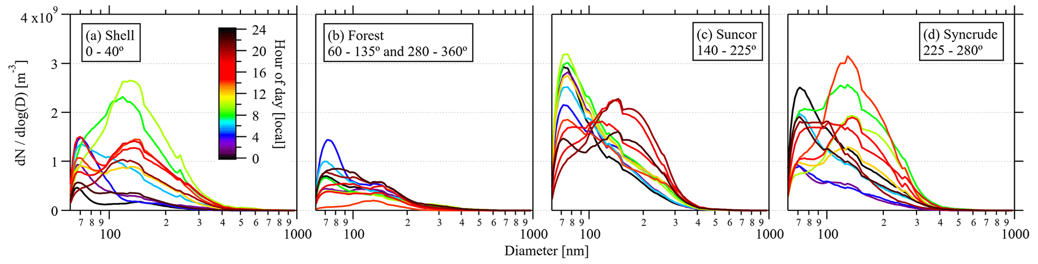
Figure 3Number particle size distributions (PSDs) by time of day (averaged over 2 h) for the four sectors identified in Fig. 2 (with the two forest sectors combined).

Figure 4Volume particle size distributions (PSDs) by time of day (averaged over 2 h) for the four sectors identified in Fig. 2 (with the two forest sectors combined).
The number PSDs (Fig. 3) do not demonstrate a consistent day–night difference across the different sectors. While morning concentrations (08:00 to 10:00) are generally highest for the three industry sources, the mode diameter of the PSDs from the Shell and Syncrude sectors is near 150 nm, while from the Suncor sector it is near 70 nm. Peak number concentration for diameters near 70 nm suggests newly formed particles from upgrader stack emissions (Zhang et al., 2018).
Howell et al. (2014) measured PSDs for number and volume from an aircraft within a plume 10 and 182 km downwind of the plume source. The particle diameter corresponding to the peak number density was approximately 15 nm at 10 km downwind and close to 60 nm at 182 km downwind. A smaller secondary peak similarly shifted from near 100 to 150 nm. Particle volume peaked between 100 and 200 nm at both 10 and 182 km downwind of the source with a secondary peak at 182 km downwind near 70 nm. At the ground level approximately 15 km from the source, we observe a number peak near 70 nm (smaller than the Howell et al., 2014, aircraft observations) and a volume peak near 250 nm (larger than the Howell et al., 2014, observations).
Baibakov et al. (2021) also measured PSD from an aircraft for two distinct plumes downwind of both the Syncrude and Suncor upgraders. One plume had significantly higher total number concentration by a factor of ∼ 2 and a peak volume near 600 nm (similar to the smaller secondary peak seen in out measurements). The lower number concentration plume had a peak volume near a diameter of 240 nm, with a volumetric PSD similar to the background (out-of-plume) PSD. Hence, YAJP surface-based results demonstrate measured plume and background PSDs with a range of distributions that show significant difference from PSDs measured from aircraft in the region.
3.2 Flux spectra
The flux spectra allow us to test whether the instrument frequency is fast enough for flux covariance and ensure that there is no substantial dispersion or diffusion in the inlet lines. Specifically, evidence of an inertial subrange at high frequencies (a variation of covariance with frequency that follows a power law) demonstrates that the eddy covariance measurement has captured the contributions of the energy-containing eddies (e.g., Foken, 2008). Normalized covariance spectra of 30 min fluxes are shown in Fig. 5, where N is the aerosol number concentration for sizes between 60 nm and 1 µm. These spectra were randomly selected from the 15–26 August period (the second half of the study when measurements were more consistent through the day). The spectra are separated into two groups according to the slope of the inertial subrange (here defined as f>0.1 Hz). The normalized co-spectra multiplied by frequency (fSwN) should vary following a power law in the inertial subrange (Kaimal and Finnigan, 1994). The spectra shown in Fig. 5a are close to this ideal, although the slope can be near −1 in some cases, possibly due to a lower signal-to-noise ratio, which can affect the co-spectral shape. Heat and CO2 fluxes measured at the site (not shown) demonstrate a power-law slope of in the inertial subrange for f>0.1 Hz. For the sample periods shown in Fig. 5b, no inertial subrange is seen, and the contribution from higher frequencies is comparable to the lower-frequency contributions. This is likely due to the flux signal being small relative to the noise caused by the instrument or diffusion in the flow direction within the sampling tube, leading to a reduced system frequency response.
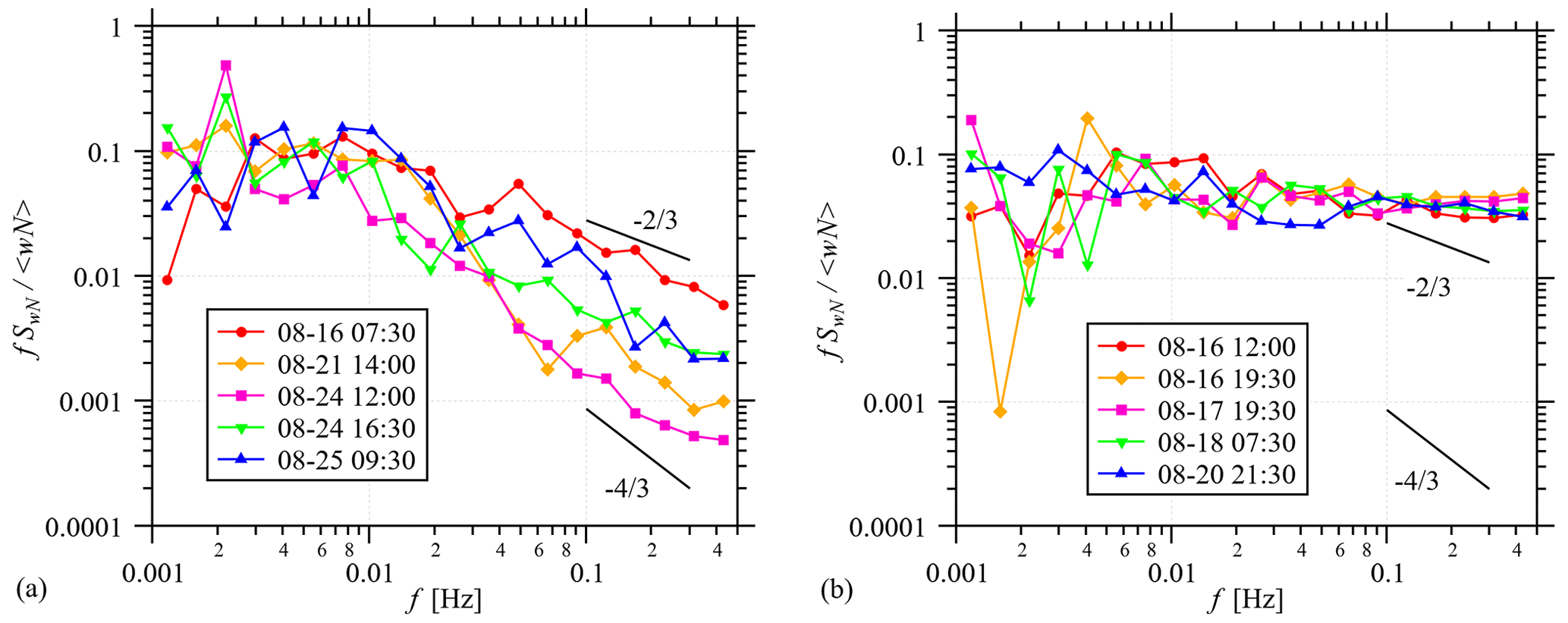
Figure 5Select aerosol number flux spectra through the measurement period demonstrating spectra with (a) an identifiable inertial subrange and (b) an unresolved inertial subrange dominated by noise. N is the total number concentration (60 nm to 1 µm) and w is the vertical velocity. The power-law slopes of and are shown for comparison. The slope is predicted by theory and the slope is used for comparative purposes.
The presence of the inertial subrange is related to the strength of the flux. Using a least-squares fit to the spectra for f>0.1 Hz, an inertial subrange slope (S) is calculated for each spectrum. The average flux magnitude for flux spectra with slopes (69 30 min values) is × 107 m−2 s−1, while the average flux magnitude for slopes (596 30 min values) is × 106 m−2 s−1 (a factor of 2.8 smaller). Similarly, the average number density is higher for the steeper slopes ( × 109 m−3 for and × 108 m−3 for ). Approximately 83 % of the spectra with are measured during the daytime (between 07:00 and 17:00) when there is greater flux of aerosols into the canopy (due to the increase in turbulent mixing during the day). This demonstrates that the presence of the inertial subrange is associated with fluxes that are greater in magnitude than the fluxes associated with flat inertial subranges (S≈0). Although the lack of an inertial subrange may indicate a significant noise-to-signal ratio, all the spectra (including those associated with lower flux and concentration values) are included in our analysis since removal of these data would introduce a daytime bias in the results.
3.3 Deposition velocity
Figure 6 shows the size-resolved deposition velocities, including average values with standard error (equivalent to 68 % confidence interval), median, and 25th and 75th percentile values. The size resolution is reduced to every third size bin to improve clarity and reduce noise (errors are averaged in quadrature). The substantial variation in the measurements is demonstrated by the 25th and 75th percentiles, which span ∼ 2 cm s−1 in the 60 to 215 nm size range. This demonstrates substantial exchange of aerosols in both directions (into and out of the canopy) with a net deposition that is a small fraction of that variation. Within the 65 to 130 nm size range vd values are not significantly different from zero in the 68 % confidence interval (CI). For the 130 to 250 nm size range vd values are significantly different from zero in the 68 % CI but would not be significantly different from zero in the 95 % CI (2 standard errors). A standard error based on the variance is used here based on the normal distribution of the measured vd values (not shown). For sizes greater than 300 nm, there is substantial variation in the values of vd between neighboring size bins, and a consistent variation of vd with size is not seen.

Figure 6Average and median deposition velocity with particle size. Error bars show standard errors of the mean (68 % confidence intervals) and the triangles show the 25th and 75th percentiles. Percentiles for diameters >300 nm are beyond the range of the graph as shown.
The average values are compared to previously published Emerson et al. (2020) measurements and parameterization in Fig. 7. Emerson et al. (2020) develop the parameterization shown in Fig. 7 based on 126 measurement points as summarized by Hicks et al. (2016), Saylor et al. (2019), and Farmer et al. (2021). The factor of 5 parameterization bounding range used by Emerson et al. (2020) and shown in Fig. 7 encloses 110 (87 %) of these previously published data points. Emerson et al. (2020) present recent size-resolved deposition velocity measurements (not included in the review papers) made using eddy covariance with a UHSAS instrument in a ponderosa pine forest. Theory predicts a minimum value in vd, which Hicks et al. (2016) refer to as a well in the size distribution of vd. The parameterization proposed by Emerson et al. (shown in Fig. 7) predicts a minimum value of vd=0.12 cm s−1 near a particle diameter of 62 nm.

Figure 7Size-resolved deposition velocities from this study (black squares) with error bars showing standard errors (68 % confidence interval). Data are overlaid on the Emerson et al. (2020) measurements (red diamonds) and parameterization (blue line with 5 × bounding range). Emerson et al. (2020) measurements are over a ponderosa pine forest, and the parameterization is for needleleaf forest (their Fig. 1).
The measurements of this study (shown as black squares in Fig. 7) show good agreement within the range of previously reported values of vd for the measured size range of 60 nm to 1 µm, particularly with the Emerson et al. (2020) results over the same size range. A local minimum of vd=0.02 cm s−1 is observed at 80 nm. Based on the standard error of the measurements, this minimum deposition velocity and many of the measurements for similar particle sizes are not significantly different from zero at the 68 % CI (error bars extending below zero in Fig. 7). The minimum measured vd=0.02 cm s−1 is much less than the modeled minimum value of vd=0.13 cm s−1 from the Emerson vd formulation and is very close to the lower limit of the parameterization bounding box, but this value is closer to the minimum measured value of Emerson et al. (2020) of vd=0.05 cm s−1 for a particle diameter near 86 nm.
3.4 Canopy decoupling and gradients
Time series measurements of particle mass concentration (PM1) made with the DustTraks at heights of 2 and 20 m demonstrate a lag between the 20 and 2 m measurements, which is more pronounced during the night. This is indicative of the decoupling between the canopy top and sub-canopy where changes in concentration due to advection above the canopy take longer to reach the sub-canopy during stable conditions (Thomas and Foken, 2007). Time lags on the order of 2 h have been observed during the night for aerosols in other forests (Gordon et al., 2011; Whitehead et al., 2010). Investigation of this effect helps to improve deposition modeling by including the decoupling effect through stability parameterizations.
The lag is determined at the YAJP site as the time a change in concentration at 20 m takes to appear in the 2 m measurement time series. Figure 8 shows the lag binned by hour of day. The jack pine boreal forest here is much less dense forest than the mixed forest of Gordon et al. (2011) or the tropical rainforest of Whitehead et al. (2010). Hence, the time lags are smaller, with peak median values near 40 min between 03:00 and 05:00. Through the afternoon, the median time lags range from 2 to 5 min.
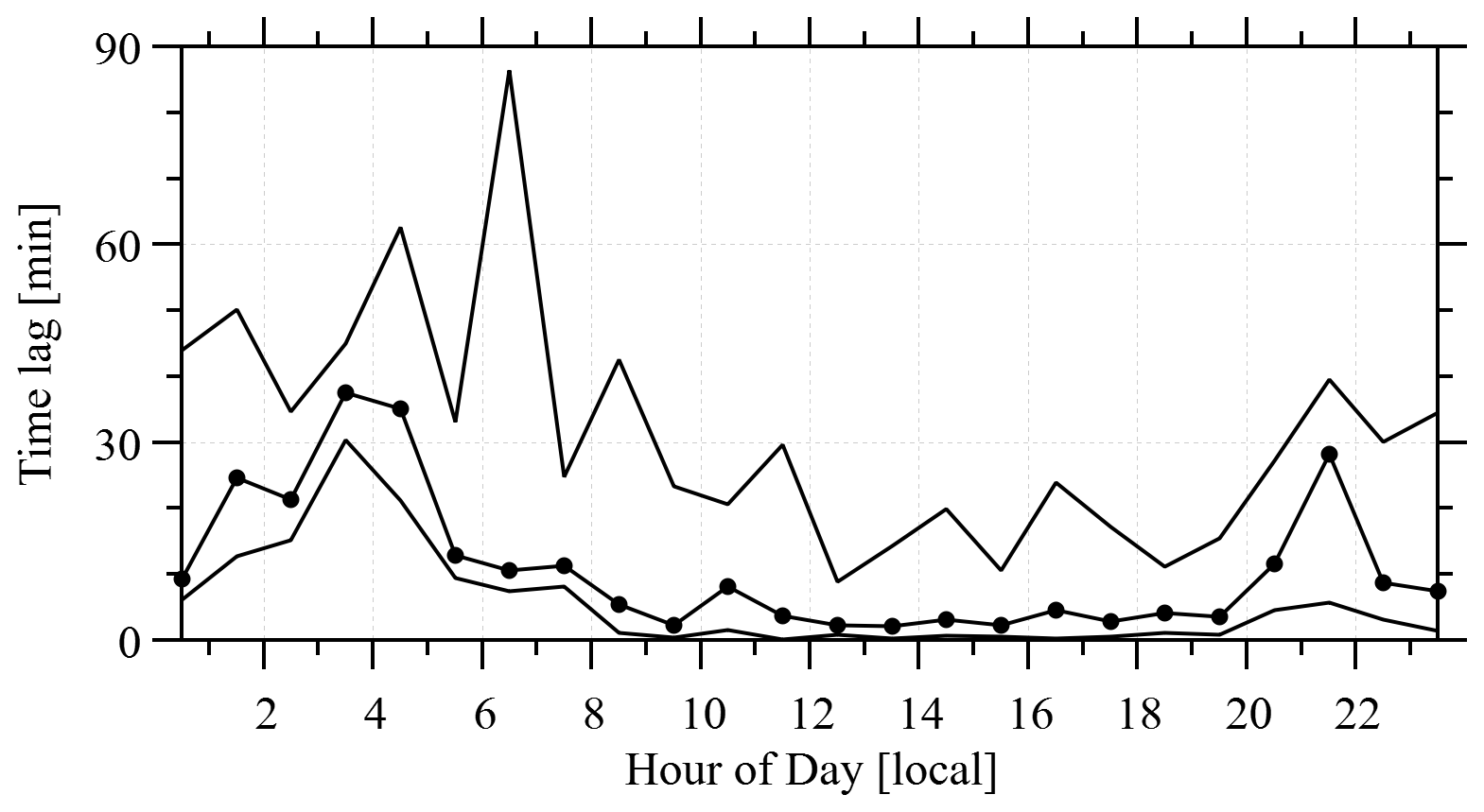
Figure 8Using the time series of TSI DustTraks the delay between changes in concentration at the canopy top and identical changes near the surface can be determined and is binned here by hour of day. Medians, 10th percentiles, and 90th percentiles are shown.
The average aerosol total PM1 mass flux (integrated over the size range of 60 nm to 1 µm) determined by eddy covariance with UHSAS measurements assuming a particle density of 1200 kg m−3 (following Emerson et al., 2020) is ng m−2 s−1 (with a 68 % CI of 5.3 ng m−2 s−1). By comparison, an average total mass flux (positive upwards) can be calculated from a two-point flux–gradient relationship as
where ΔC is the concentration difference between two heights separated by Δz, and K is the average diffusion coefficient between the two heights.
One approach is to parameterize K based on a measured two-point wind gradient and momentum flux (You et al., 2021, and Gordon et al., 2022). Here Prandtl's mixing length model is adjusted for stability following Garratt (1994) to give
where κ=0.4 is the von Kármán constant, zm is a representative flux measurement height, Sc=0.8 is the turbulent Schmidt number (ratio of momentum diffusion to trace gas diffusion), u∗ is the friction velocity, and ϕ is a stability parameter. The stability parameter (ϕ) is determined from the Obukhov length (L) following Garratt (1994) as
In cases of closed canopies, flux–gradient relationships are not generally applicable inside the canopy due to counter-gradient fluxes and modified stability within the canopy (Thomas and Foken, 2007). Measurements at this forest tower site outlined in Gordon et al. (2022) demonstrate good agreement (R2=0.83) between K determined by the measured flux and the gradient with a representative height of zm=11 m, which is roughly the middle of the canopy height (hc=19 m). This good agreement at this site may be due to the relative openness of the canopy (Fig. 1b).
Another approach specific to forest canopies uses a vertically varying diffusion coefficient following Raupach (1988) as , where the Lagrangian timescale and is the vertical velocity variance, which varies with height. If it is assumed that σw varies linearly from zero at the surface up to a value of σw(zm) at height zm, then the average K over the height of the canopy is
Makar et al. (2017) also propose a vertically varying K(z) parameterization specific to forest canopies based on measurements from a number of studies (references therein). Here we vertically average this parameterization through the canopy height to give
where is a function based on the Obukhov length (L). The function is nearly linear between f=2.35 m at and f=0.38 m for and is constant outside those limits.
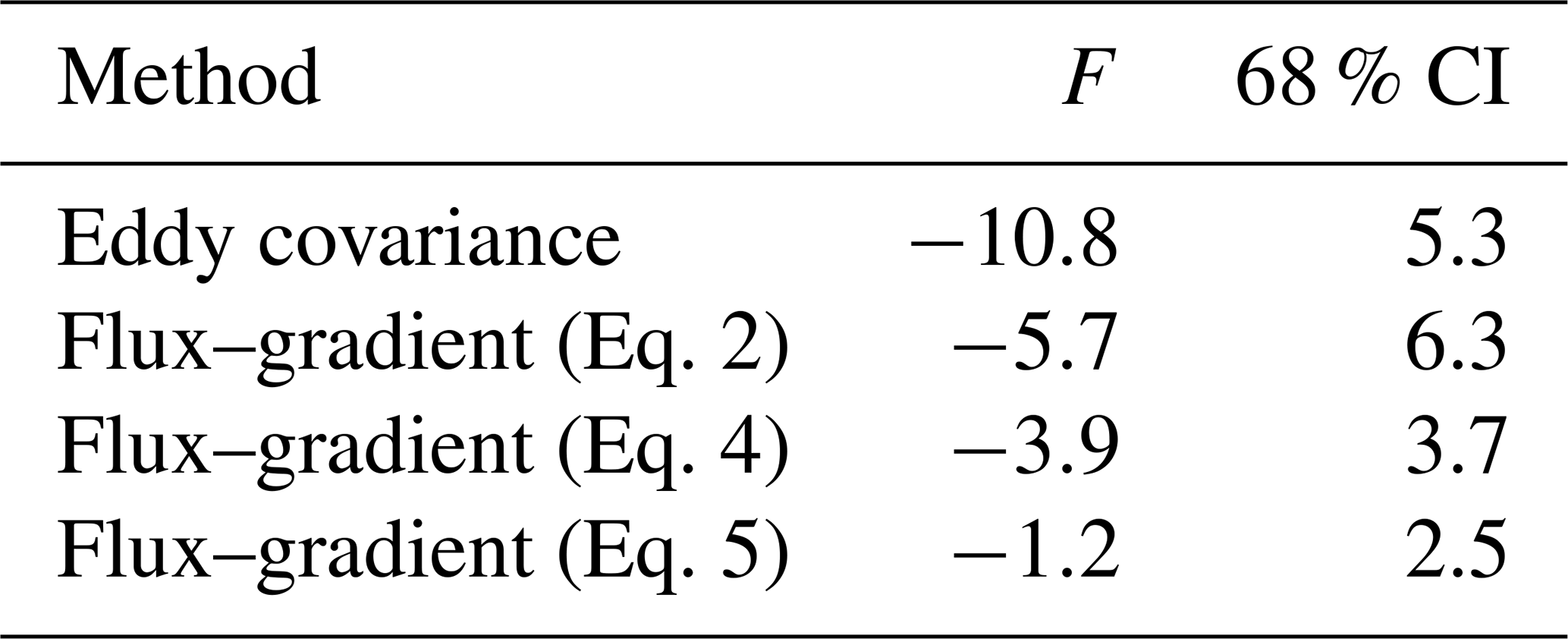
Table 1 compares the flux calculated using the flux–gradient method using these three diffusion parameterizations (Eqs. 2–5) against the average PM1 mass flux calculated with eddy covariance. The concentration difference ΔC is calculated using the PM1 mass concentration measured by the DustTraks (integrated from 0.1 to 1 µm) with the 0.5 correction factor discussed in Sect. 2.1. The values are constantly smaller in magnitude than the eddy covariance flux by a factor ranging from 2 (Eq. 2) to 9 (Eq. 5). Due to the relatively small differences between the upper and lower concentrations, there is a large amount of noise in the gradient () and only two of the three flux–gradient averages are significantly different from zero at the 68 % CI.
Table 1Average PM1 mass flux measured by eddy covariance compared to the average mass flux from two-point flux–gradient measurements using different K parameterizations. The confidence interval (CI) is given as the standard error of the mean (all units are ng m−2 s−1.)
These differences may be due to the oversimplification of the two-point gradient approximation, which does not account for modification of in-canopy stability or counter-gradient fluxes. In addition to potential vertical variation in K, there may also be vertical variation in deposition resistance () throughout the canopy. The two-point gradient approximation only assumes deposition to the forest floor and not the tree and leaf surfaces. Any deposition which occurs within the canopy would likely reduce the concentration gradient and hence lead to an underestimation of K, which here is based on aerodynamic resistance only.
Regardless of the cause, this implies that the diffusion coefficients estimated using a two-point gradient are likely underestimated. This also demonstrates the degree of uncertainty involved in parameterizing a diffusion coefficient through the vertical extent of the canopy since the 68 % CI is close in magnitude to (or greater than) the average flux values.
YAJP surface-based results demonstrated measured plume and background PSDs with a range of distributions that show significant difference from PSDs measured from aircraft in the region. Measurements suggest that larger (>500 nm diameter) particles are from open-pit mining to the north of the tower and smaller (<100 nm diameter) particles are from stack sources from the west and southwest directions. Aerosols from the direction of mining and processing facilities showed number concentration peaks near 70 and 150 nm and volume distribution peaks near 250 nm (with secondary peaks near 600 nm).
Aerosol flux measurements on the tower demonstrate substantial exchange of aerosols in both directions (into and out of the canopy) when averaged to 30 min fluxes. The net deposition over the nearly month-long measurement period is a small fraction of that variation. Deposition results agree with previous studies measuring aerosol deposition over forests in the <1 µm size range. A local minimum of vd=0.02 cm s−1 is observed at 80 nm, which is slightly less than the range suggested by the Emerson et al. (2020) parameterization, but not significantly different from this range (i.e., overlapping within the range of measurement uncertainty).
The local minimum of deposition velocity for sizes near 80 nm corresponds to the peak size (near 70 nm) of the number concentration PSD, presumably from smokestack emissions. This demonstrates the importance of correctly modeling deposition velocity in this range to accurately measure the number of particles depositing to forests. However, PSDs demonstrate that the bulk of mass (of submicron particles) is in the 150 to 400 nm range (or the 150 to 700 nm range for sources with open-pit mining emissions), so most of the aerosol mass deposited to the forest is likely due to impaction and interception by leaves and surfaces due to particle inertia.
Decoupling of the forest canopy is demonstrated at nighttime, with median lag times for concentration changes to be communicated from above the canopy to near the surface of up to 40 min. Median time lags during the day are between 2 and 5 min. The use of the flux–gradient method with the measured aerosol concentration gradient gives a size-integrated mass flux of PM1, which is between a factor of 2 and 9 smaller in magnitude than the flux measured by eddy covariance, depending on the parameterization used for the diffusion coefficient, K. The uncertainties in the averages determined by the flux–gradient method are comparable in magnitude to the averages (at the 68 % CI), which demonstrates the substantial uncertainty in determining an average flux using the flux–gradient method.
Based on these results, it is recommended to use a more detailed modeling approach, such as the high-resolution, one-dimensional canopy model outlined in Zhang et al. (2023), to investigate the relationship between time lags in the canopy and the modeled diffusion coefficients. This could help to determine if parameterizations of K(z) can accurately reproduce the time lags seen in this and other studies and ensure that canopy decoupling can be accurately represented through diffusion-based modeling. This could potentially improve the agreement between the flux–gradient estimations and the eddy covariance measurements for PM1 at this location.
The data described in this study are available at https://doi.org/10.5683/SP3/CT4WFO (Gordon, 2023).
TJ and MG wrote the original draft of this work and performed the analysis. MG and PM conceptualized the field study. PM acquired funding. MG and TJ performed the field experiments. MW, MG, and TJ performed instrument calibration and laboratory tests. PM, RS, and MW reviewed and edited the work.
The contact author has declared that none of the authors has any competing interests.
Publisher's note: Copernicus Publications remains neutral with regard to jurisdictional claims in published maps and institutional affiliations.
We acknowledge the technical support and assistance of the Wood Buffalo Environment Association (WBEA) of Alberta.
This research has been supported by Environment and Climate Change Canada (grant no. GCXE20S044).
This paper was edited by Tuukka Petäjä and reviewed by Bruce Hicks and one anonymous referee.
Adams, E. E.: World Forest Area Still on the Decline, Earth Policy Institute, http://www.earth-policy.org/mobile/releases/forests_2012 (last access: 6 April 2023), 2012
Baibakov, K., LeBlanc, S., Ranjbar, K., O'Neill, N. T., Wolde, M., Redemann, J., Pistone, K., Li, S.-M., Liggio, J., Hayden, K., Chan, T. W., Wheeler, M. J., Nichman, L., Flynn, C., and Johnson, R.: Airborne and ground-based measurements of aerosol optical depth of freshly emitted anthropogenic plumes in the Athabasca Oil Sands Region, Atmos. Chem. Phys., 21, 10671–10687, https://doi.org/10.5194/acp-21-10671-2021, 2021.
Boucher, O., Randall, D., Artaxo, P., Bretherton, C., Feingold, G., Forster, P., Kerminen, V.-M., Kondo, Y., Liao, H., Lohmann, U., Rasch, P., Satheesh, S. K., Sherwood, S., Stevens, B., and Zhang, X. Y.: Clouds and Aerosols, in: Climate Change 2013: The Physical Science Basis. Contribution of Working Group I to the Fifth Assessment Report of the Intergovernmental Panel on Climate Change, edited by: Stocker, T. F., Qin, D., Plattner, G.-K., Tignor, M., Allen, S. K., Boschung, J., Nauels, A., Xia, Y., Bex, V., and Midgley, P. M., Cambridge University Press, Cambridge, United Kingdom and New York, NY, USA, 571–658, https://doi.org/10.1017/CBO9781107415324.016, 2013.
Cai, Y., Montague, D. C., Mooiweer-Bryan, W., and Deshler, T.: Performance characteristics of the ultra high sensitivity aerosol spectrometer for particles between 55 and 800 nm: Laboratory and field studies, J. Aerosol Sci., 39, 759–769, https://doi.org/10.1016/j.jaerosci.2008.04.007, 2008.
Davidson, C. and Spink, D.: Alternate approaches for assessing impacts of oil sands development on air quality: A case study using the First Nation Community of Fort McKay, J. Air Waste Manage., 68, 308–328, https://doi.org/10.1080/10962247.2017.1377648, 2018.
Emerson, E. W., Hodshire, A. L., DeBolt, H. M., Bilsback, K. R., Pierce, J. R., McMeeking, G. R., and Farmer, D. K.: Revisiting particle dry deposition and its role in radiative effect estimates, P. Natl. Acad. Sci. USA, 117, 26076–26082, https://doi.org/10.1073/pnas.2014761117, 2020.
Farmer, D. K., Boedicker, E. K., and DeBolt, H. M.: Dry Deposition of Atmospheric Aerosols: Approaches, Observations, and Mechanisms, Annu. Rev. Phys. Chem., 72, 375–97, https://doi.org/10.1146/annurev-physchem-090519-034936, 2021.
Foken, T.: Micrometeorology, Springer, Berlin, https://doi.org/10.1007/978-3-540-74666-9, 2008.
Frazer, G. W., Canham, C. D., and Lertzman, K. P.: Gap Light Analyzer (GLA), Version 2.0: Imaging software to extract canopy structure and gap light transmission indices from true-colour fisheye photographs, users manual and program documentation, Copyright © 1999: Simon Fraser University, Burnaby, British Columbia, and the Institute of Ecosystem Studies, Millbrook, New York, 1999.
Garratt, J. R.: The Atmospheric Boundary Layer, edited by: Houghton, J. T., Rycroft, M. J., and Dessler, A. J., Cambridge University Press, ISBN-10 0521467454, ISBN-13 978-0521467452, 1994.
Gordon, M.: Aerosol measurements in the boreal forest in the vicinity of the Alberta Oil Sands, V1, Borealis [data set], https://doi.org/10.5683/SP3/CT4WFO, 2023
Gordon, M., Staebler, R. M., Liggio, J., Vlasenko, A., Li, S.-M., and Hayden, K.: Aerosol flux measurements above a mixed forest at Borden, Ontario, Atmos. Chem. Phys., 11, 6773–6786, https://doi.org/10.5194/acp-11-6773-2011, 2011.
Gordon, M., Blanchard, D., Jiang, T., Makar, P. A., Staebler, R. M., Aherne, J., Mihele, C., and Zhang, X.: High sulphur dioxide deposition velocities measured with the flux/gradient technique in a boreal forest in the Alberta oil sands region, Atmos. Chem. Phys. Discuss. [preprint], https://doi.org/10.5194/acp-2022-668, in review, 2022.
Hicks, B. B., Saylor, R. D., and Baker, B. D.: Dry deposition of particles to canopies – A look back and the road forward. J. Geophys. Res.-Atmos., 121, 14691–14707, https://doi.org/10.1002/2015JD024742, 2016.
Horst, T. W.: A simple formula for attenuation of eddy fluxes measured with first-order-response scalar sensors, Bound.-Lay. Meteorol., 82, 219–233, https://doi.org/10.1023/A:1000229130034, 1997.
Howell, S. G., Clarke, A. D., Freitag, S., McNaughton, C. S., Kapustin, V., Brekovskikh, V., Jimenez, J.-L., and Cubison, M. J.: An airborne assessment of atmospheric particulate emissions from the processing of Athabasca oil sands, Atmos. Chem. Phys., 14, 5073–5087, https://doi.org/10.5194/acp-14-5073-2014, 2014.
Kaimal, J. C. and Finnigan, J. J.: Atmospheric Boundary-Layer Flows: Their Structure and Measurement, Oxford University Press, ISBN 9780195062397, 1994.
Kappos, A. D., Bruckmann, P., Eikmann, T., Englert, N., Heinrich, U., Höppe, P., Koch, E., Krause, G. H. M., Kreyling, W. G., Rauchfuss, K., Rombout, P., Schulz-Klemp, V., Thiel, W. R., and Wichmann, H.-E.: Health Effects of Particles in Ambient Air, Int. J. Hyg. Environ. Health, 207, 399–407, https://doi.org/10.1078/1438-4639-00306, 2004.
Liggio, J., Li, S.-M., Hayden, K., Taha, Y. M., Stroud, C., Darlington, A., Drollette, B. D., Gordon, M., Lee, P., Liu, P., Leithead, A., Moussa, S. G., Wang, D., O'Brien, J., Mittermeier, R. L., Brook, J. R., Lu, G., Staebler, R. M., Han, Y., Tokarek, T. W., Osthoff, H. D., Makar, P. A., Zhang, J., Plata, D. L., and Gentner, D. R.: Oil sands operations as a large source of secondary organic aerosols, Nature, 534, 91–94, https://doi.org/10.1038/nature17646, 2016.
Makar, P. A., Staebler, R. M., Akingunola, A., Zhang, J., Mclinden, C., Kharol, S. K., Pabla, B., Cheung, P., and Zheng, Q.: The effects of forest canopy shading and turbulence on boundary layer ozone, Nat. Commun., 8, 15243, https://doi.org/10.1038/ncomms15243, 2017.
Mammarella, I., Rannik, U., Aalto, P., Keronen, P., Vesala, T., and Kulmala, M.: Long-term aerosol particle flux observations. Part II: Particle size statistics and deposition velocities, Atmos. Environ., 45, 3794–3805, https://doi.org/10.1016/j.atmosenv.2011.04.022, 2011.
Matsuda, K.: Dry deposition of aerosols onto forest, in: Air Pollution Impacts on Plants in East Asia, edited by: Izuta, T., Springer, Tokyo, 309–322, https://doi.org/10.1007/978-4-431-56438-6, 2017.
Natural Resources Canada (NRCan): The state of Canada's forests, annual report 2021, Natural Resources Canada, Canadian Forest Service, Ottawa, Canada, ISSN 1196-1589, 2021.
Petroff, A., Murphy, J. G., Thomas, S. C., and Geddes, J. A.: Size-resolved aerosol fluxes above a temperate broadleaf forest, Atmos. Environ., 190, 359–375, https://doi.org/10.1016/j.atmosenv.2018.07.012, 2018.
Pryor, S. C., Barthelmie, R. J., Sørensen, L. L., Larsen, S. E., Sempreviva, A. M., Grönholm, T., Rannik, U., Kulmala, M., and Vesala, T.: Upward fluxes of particles over forests: when, where, why?, Tellus B, 60, 372–380, https://doi.org/10.1111/j.1600-0889.2008.00341.x, 2008.
Rannik, Ü., Vesala, T., and Keskinen, R.: On the dampening of temperature fluctuations in a circular tube relevant to eddy covariance measurement technique, J. Geophys. Res., 102, 12789–12794, https://doi.org/10.1029/97JD00362, 1997.
Raupach, M. R.: Turbulent transfer in plant canopies, in Plant Canopies – Their Growth, Form and Function, edited by: Russell, G., Marshall, B., and Jarvis, P. G., Cambridge Univ. Press, New York, ISBN 9780521395632, 41–61, 1988.
Saylor, R. D., Baker, B. D., Lee, P., Tong, D., Pan, L., and Hicks, B. H.: The particle dry deposition component of total deposition from air quality models: right, wrong or uncertain?, Tellus B, 71, 1550324, https://doi.org/10.1080/16000889.2018.1550324, 2019.
Schilperoort, B., Coenders-Gerrits, M., Jiménez Rodríguez, C., van der Tol, C., van de Wiel, B., and Savenije, H.: Decoupling of a Douglas fir canopy: a look into the subcanopy with continuous vertical temperature profiles, Biogeosciences, 17, 6423–6439, https://doi.org/10.5194/bg-17-6423-2020, 2020.
Thomas, C. and Foken, T.: Flux contribution of coherent structures and its implications for the exchange of energy and matter in a tall spruce canopy, Bound.-Lay. Meteorol., 123, 317–337, https://doi.org/10.1007/s10546-006-9144-7, 2007.
You, Y., Staebler, R. M., Moussa, S. G., Beck, J., and Mittermeier, R. L.: Methane emissions from an oil sands tailings pond: a quantitative comparison of fluxes derived by different methods, Atmos. Meas. Tech., 14, 1879–1892, https://doi.org/10.5194/amt-14-1879-2021, 2021.
Webb, E. K., Pearman, G., and Leuning, R.: Correction of the flux measurements for density effects due to heat and water vapour transfer, Q. J. Roy. Meteor. Soc., 106, 85–100, https://doi.org/10.1002/qj.49710644707, 1980.
Whitehead, J. D., Gallagher, M. W., Dorsey, J. R., Robinson, N., Gabey, A. M., Coe, H., McFiggans, G., Flynn, M. J., Ryder, J., Nemitz, E., and Davies, F.: Aerosol fluxes and dynamics within and above a tropical rainforest in South-East Asia, Atmos. Chem. Phys., 10, 9369–9382, https://doi.org/10.5194/acp-10-9369-2010, 2010.
Wilczak, J. M., Oncley, S. P., and Stage, S. A.: Sonic anemometer tilt correction algorithms, Bound.-Lay. Meteorol., 99, 127–150, https://doi.org/10.1023/A:1018966204465, 2001.
Yousif, M., Brook, J. R., Evans, G. J., Jeong, C.-H., Jiang, Z., Mihele, C., Lu, G., and Staebler, R. M.: Source Apportionment of Volatile Organic Compounds in the Athabasca Oil Sands Region, https://doi.org/10.2139/ssrn.4181135, 2022.
Yun, D. M., Kim, M. B., Lee, J. B., Kim, B. K., Lee, D. J., Lee, S. Y., Yu, S., and Kim, S. R.: Correction factors for outdoor concentrations of PM2.5 measured with portable real-time monitors compared with gravimetric methods: Results from South Korea, Journal of Environmental Science International, 24, 1559–1567, https://doi.org/10.5322/JESI.2015.24.12.1559, 2015.
Zhang, J., Moran, M. D., Zheng, Q., Makar, P. A., Baratzadeh, P., Marson, G., Liu, P., and Li, S.-M.: Emissions preparation and analysis for multiscale air quality modeling over the Athabasca Oil Sands Region of Alberta, Canada, Atmos. Chem. Phys., 18, 10459–10481, https://doi.org/10.5194/acp-18-10459-2018, 2018.
Zhang, L. M., Gong, S. L., Padro, J., and Barrie, L.: A size-segregated particle dry deposition scheme for an atmospheric aerosol module, Atmos. Environ., 35, 549–560, https://doi.org/10.1016/S1352-2310(00)00326-5, 2001.
Zhang, X., Gordon, M., Makar, P. A., Jiang, T., Davies, J., and Tarasick, D.: Ozone in the boreal forest in the Alberta oil sands region, Atmos. Chem. Phys. Discuss. [preprint], https://doi.org/10.5194/acp-2023-26, in review, 2023.