14 years of lidar measurements of polar stratospheric clouds at the French Antarctic station Dumont d'Urville

Polar stratospheric clouds (PSCs) play a critical role in the stratospheric ozone depletion processes. The last 30 years have seen significant improvements in our understanding of the PSC processes but PSC parametrization in global models still remains a challenge due to the necessary trade-off between the complexity of PSC microphysics and model parametrization constraints. The French Antarctic station Dumont d'Urville (DDU, 66.6^∘ S, 140.0^∘ E) has one of the few high latitude ground-based lidars in the Southern Hemisphere that has been monitoring PSCs for decades. This study focuses on the PSC data record during the 2007–2020 period. First, the DDU lidar record is analysed through three established classification schemes that prove to be mutually consistent: the PSC population observed above DDU is estimated to be of 30 % supercooled ternary solutions, more than 60 % nitric acid trihydrate mixtures and less than 10 % of water–ice dominated PSC. The Cloud–Aerosol Lidar with Orthogonal Polarization PSC detection around the station are compared to DDU PSC datasets and show a good agreement despite more water–ice PSC detection. Detailed 2015 lidar measurements are presented to highlight interesting features of PSC fields above DDU. Then, combining a temperature proxy to lidar measurements, we build a trend of PSC days per year at DDU from ERA5 (the fifth generation of European ReAnalysis) and NCEP (National Centers for Environment Protection reanalysis) reanalyses fitted on lidar measurements operated at the station. This significant 14-year trend of −4.6 PSC days per decade is consistent with recent temperature satellite measurements at high latitudes. Specific DDU lidar measurements are presented to highlight fine PSC features that are often sub-scale to global models and spaceborne measurements.

1 Introduction

Polar stratospheric clouds (PSCs) have been closely investigated for several decades, primarily due to their critical role in stratospheric ozone chemistry. PSC particles are a combination of water vapour (H₂O), nitric acid (HNO₃) and sulfuric acid (H₂SO₄) in different physical states and are often observed as layers featuring different chemical compositions. They form during the winter polar stratosphere when the temperature decreases below specific thresholds related to nitric acid and water vapour freezing points. Their main impact is to enable heterogeneous chemical reactions that convert stable chlorine and bromine reservoirs into active radicals that catalytically deplete ozone in the presence of sunlight (Solomon, 1999). Denitrification and dehydration, mostly through the uptake of HNO₃ and H₂O by PSCs and the subsequent PSC sedimentation, decrease HNO₃ and H₂O stratospheric concentration and hence enhance ozone depletion (WMO, 2018). Despite major improvements in the recent years due to enhanced research and monitoring capabilities, some PSC-related aspects are still to be understood. Spatial measurements brought a global point of view able to grasp the spatial and temporal distribution of PSC during winter (Pitts et al., 2018). Studies highlighted the need to take wave-induced temperature variations into account to adequately model PSC occurrences (Cairo et al., 2004; Höpfner et al., 2006; Eckermann et al., 2006; Engel et al., 2013; Tritscher et al., 2019). However, some PSC particle formation pathways are still debated (Tritscher et al., 2021) and the adequate model parametrization of PSCs is still challenging. Besides, the recent stratospheric injections of aerosols caused by volcanic eruptions and wildfires also raise questions on the potential interaction with PSC formation processes and subsequent stratospheric ozone depletion (Tencé et al., 2022; Ansmann et al., 2022; Rieger et al., 2021; Stone et al., 2021).

Depending on pressure, temperature H₂O and HNO₃ gas phase concentrations, and possibly on the abundance of available nuclei, the three key species combine and form different types of particles and clouds. The nuclei are generally stratospheric sulfuric acid aerosols or to a lesser extent meteoritic material, whose role in PSC particles nucleation is still a subject of discussion (Ebert et al., 2016; James et al., 2018). Water–ice crystals (ICE), nitric acid trihydrate (NAT) and supercooled ternary solution droplets (STSs) of H₂O, HNO₃ and H₂SO₄ are the three particle types which have been fully characterized in laboratory studies (Koop et al., 2000; Hanson and Mauersberger, 1988; Carslaw et al., 1997). Ice particles can nucleate both homogeneously and heterogeneously depending on the temperature and air mass history, while NAT particles only nucleate on pre-existing particles (Koop et al., 1995, 1997; James et al., 2018). STS droplets form by the uptake of atmospheric gas phase HNO₃ by sulfuric acid aerosols. PSCs are generally composed of a mixture of these base particles. Depending on their dominant type of particles, different PSCs have different surface area densities and chemical heterogeneous reactivities and therefore different levels of halogen activation. Ice crystals are known to be the most efficient in chlorine activation. However, since they are relatively rare, most of the chlorine activation occurs on or in liquid particles (Abbatt and Molina, 1992; Hanson and Ravishankara, 1993; Wegner et al., 2012; Tritscher et al., 2021). The efficiencies of STS, NAT, ICE particles and stratospheric aerosols to activate chlorine are compared as a function of temperature in Fig. 39 of Tritscher et al. (2021).

From these three basic particle types and their combinations, more detailed types of PSCs were identified for the purpose of creating classifications based on optical properties of the pure STS, NAT and ICE blends of chemical compounds. The first was published by Poole and McCormick (1988). Since then, several classifications have been proposed, listing different types of clouds based on different sets of variables (Browell et al., 1990; Toon et al., 1990; Stein et al., 1999; Santacesaria et al., 2001; Adriani et al., 2004; Massoli et al., 2006; Blum et al., 2005; Pitts et al., 2009, 2011, 2013, 2018). Over the years, these schemes became more complex as STS, NAT and ICE base types could not explain alone the full extent of observed PSC characteristics and resulted in high proportions of unclassified measurements (up to 30 %; Achtert and Tesche, 2014). Additionally, some of the early classification schemes included thermodynamically unstable species at stratospheric conditions which were sometimes detected in laboratory experiments, notably sulfuric acid tetrahydrate (SAT) or nitric acid dihydrate (NAD), but have yet to be confirmed by atmospheric observations. Studies showed that PSC type identification depends on the history of the air masses due to hysteresis effects on PSC formation along the temperature scale (Larsen, 2000). In addition, the temperature cooling rate is an important variable driving orographic PSC formation in both the Arctic and Antarctic (Noel and Pitts, 2012).

Overall, the modelling community has not been able to take full advantage of complex PSC classification schemes as most models often have only a few variables to resolve PSC microphysics. Therefore, the combination of model constraints and the high rate of unclassified observations (due to either instrumental concerns or unequilibrated particles) led to some redefinition of the boundaries between the existing PSC classes rather than considering additional classes. The PSC classification schemes previously mentioned are based on ground-based or spaceborne lidar measurements. While in situ measurements with balloons or stratospheric aircraft are highly valuable, they remain rare. Lidar instruments, both ground-based and spaceborne, are more appropriate to study PSCs as they provide extremely high vertical and time resolution data at the cost of a heavy inversion procedure (i.e. as compared to direct particle counters) needed to retrieve the optical properties.

Achtert and Tesche (2014) presented a comprehensive review of the PSC classification schemes. Their study shows that these classifications can lead to very different outcomes when applied to a single dataset. As these classifications are often derived from a single instrument, they are likely to carry their own biases and prevent quantitative comparisons with other datasets carrying other biases related to different instrumental setups. Also, different sets of variables have been used to interpret the measurements and the lack of homogeneity in lidar data processing and in the definition of some optical properties make intercomparisons between different studies more difficult. Following the conclusions of Achtert and Tesche (2014), we decided to consider three different classifications proposed by Blum et al. (2005) (hereafter called B05), Pitts et al. (2011) (hereafter called P11), and an updated version of P11 (Pitts et al., 2018, hereafter called P18).

These classifications are used to analyse the lidar measurements conducted at the French Antarctic station Dumont d'Urville (DDU, 66.6^∘ S, 140.0^∘ E). DDU is located on the shore of the continent and therefore often lies at the edge of the polar vortex. The station has hosted a stratospheric lidar since 1989, making it one of the very few Antarctic station with a long-term lidar data record. Considering the latest laser source replacement in 2005 and the continuous monitoring from 2006, DDU PSC dataset is compared to the spaceborne PSC measurements conducted by CALIOP (Cloud–Aerosol Lidar with Orthogonal Polarization) in the vicinity of the station, from 2007 to 2020. Two of the major roles of a ground station are to perform process studies and establish decadal trends. Such trends are highly valuable because they reflect the evolution of the stratosphere in terms of temperature and chemical compositions. In this study, DDU lidar measurements are exploited to produce a trend of PSC days per year at DDU.

Section 2 presents the data and instruments exploited in this study. Section 3 introduces the PSC detection methods as well as the considered classification schemes. Section 4 exposes the results of the study. First, the outcomes of the application of the classification schemes B05, P11 and P18 to the DDU lidar data record are presented and discussed, and CALIOP and DDU PSC measurements are compared. Then the analysis of an interesting example of a long lidar session is used to illustrate the unique capabilities of lidar measurements in characterizing very fine vertical features in PSC fields. Third, lidar measurements and temperatures from ERA5 (the fifth generation of European ReAnalysis), NCEP (National Centers for Environment Protection reanalysis) and infrared atmospheric sounding interferometers (IASIs) are combined to produce a PSC occurrence trend from 2007 to 2020. To support the use of these temperature data sources, they are compared to temperatures from radiosondes launched daily at DDU. Finally, some challenges of PSC parametrization in climate models are discussed before exposing the main conclusions.

2 Data and instruments

2.1 Dumont d'Urville Lidar

An aerosol/cloud lidar system has been in operation at DDU since April 1989 in the framework of the Network for Detection of Atmospheric Composition Changes (NDACC). Originally designed as a PSC monitoring instrument, its capabilities have been extended to study aerosol/cirrus clouds in the Antarctic atmosphere, benefiting from continuous technological upgrades of its different subsystems. Although the measurement calendar focuses on the PSC season with nighttime setup, recent work on aerosol plumes either originating from volcanic or biomass burning activity (Tencé et al., 2022) suggests extending the measurement calendar to the summertime. Figure 1 shows the amount and duration of the lidar measurement sessions. Figure 1a shows the recent increase in amount of measurements triggered by the new focus on aerosol plumes detection. Figure 1b shows that while 90 min is the minimum duration of operation, sessions can reach more than 6 h during winter.

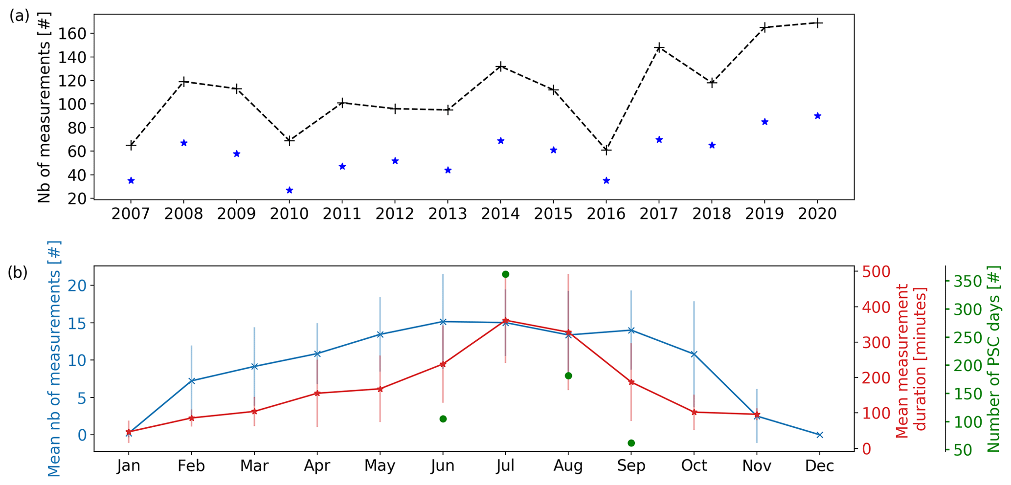
Figure 1 Operation statistics of DDU lidar. (a) Number of measurement days per year (black line) and per winter (blue stars) from 2007 to 2020 and (b) mean number (blue line) and duration (red line) of measurement sessions per month, in minutes, from 2007 to 2020. Total number of PSC days at DDU in June, July, August and September between 2007 and 2020 (green circles).

The Rayleigh/Mie/Raman lidar operates at the 532 nm wavelength. N₂ vibrational Raman backscattering at 607 nm is also acquired. An extensive description of both the instrumental design and inversion procedure is featured in David et al. (2012). The Nd:YAG laser source emits at 10 Hz frequency with around 250 mJ emitted power in the visible. Backscattered photons are collected on a collocated 80 cm diameter Newton telescope. A polarizing cube at the reception splits the beam into two components polarized parallel and perpendicular to the laser emission for the 532 nm wavelength; each component is recorded and inverted to gain access to the depolarization ratio. In this study, we use the aerosol depolarization value defined as the ratio between the perpendicular and parallel particulate backscatter coefficients. Aerosol vertical profiles will be considered as Backscatter Ratio or Scattering Ratio profiles (hereafter called R_T) expressed as the ratio of the total backscattering (i.e. including Mie Scattering) to the molecular backscattering at a given altitude. The different lidar-related variables used in this study are defined as follows, as a function of the parallel and perpendicular molecular backscatter coefficients (${\mathit{\beta }}_{\mathrm{mol},\parallel }$ and ${\mathit{\beta }}_{\mathrm{mol},⟂}$ respectively) and of the parallel and perpendicular particulate backscatter coefficients (${\mathit{\beta }}_{\mathrm{aer},\parallel }$ and ${\mathit{\beta }}_{\mathrm{aer},⟂}$ respectively):

$$\begin{array}{}\text{(1)}& R_T={\displaystyle \frac{{\mathit{\beta }}_{\mathrm{aer},\parallel }+{\mathit{\beta }}_{\mathrm{aer},⟂}+{\mathit{\beta }}_{\mathrm{mol},\parallel }+{\mathit{\beta }}_{\mathrm{mol},⟂}}{{\mathit{\beta }}_{\mathrm{mol},\parallel }+{\mathit{\beta }}_{\mathrm{mol},⟂}}}.\end{array}$$

The parallel and perpendicular backscatter ratio (R_∥ and R_⟂), are defined as

$$\begin{array}{}\text{(2)}& {\displaystyle }{R}_{\parallel }={\displaystyle \frac{{\mathit{\beta }}_{\mathrm{aer},\parallel }+{\mathit{\beta }}_{\mathrm{mol},\parallel }}{{\mathit{\beta }}_{\mathrm{mol},\parallel }}}\text{(3)}& {\displaystyle }{R}_{⟂}={\displaystyle \frac{{\mathit{\beta }}_{\mathrm{aer},⟂}+{\mathit{\beta }}_{\mathrm{mol},⟂}}{{\mathit{\beta }}_{\mathrm{mol},⟂}}}.\end{array}$$

The linear particle depolarization ratio is defined as

$$\begin{array}{}\text{(4)}& {\mathit{\delta }}_{\mathrm{aer}}={\displaystyle \frac{{\mathit{\beta }}_{\mathrm{aer},⟂}}{{\mathit{\beta }}_{\mathrm{aer},\parallel }}}={\displaystyle \frac{R_{⟂}-\mathrm{1}}{R_{\parallel }-\mathrm{1}}}{\mathit{\delta }}_{\mathrm{mol}},\end{array}$$

where ${\mathit{\delta }}_{\mathrm{mol}}=\frac{{\mathit{\beta }}_{\mathrm{mol},⟂}}{{\mathit{\beta }}_{\mathrm{mol},\parallel }}$ is the depolarization ratio of the molecular background and depends on the lidar used. Depending on the width of the interference filter used on the 532 nm channel, some lidars only detect the central Cabannes line, while other instruments also detect the shifted Raman lines. The interference filter used for DDU lidar has a full width at half maximum (FWHM) of 1 nm bandwidth, and therefore the corresponding molecular depolarization parameter is set to δ_mol=0.443 % (Behrendt and Nakamura, 2002).

Finally, the total perpendicular backscatter coefficient can be expressed as follows:

$$\begin{array}{}\text{(5)}& {\mathit{\beta }}_{\mathrm{tot},⟂}={\mathit{\beta }}_{\mathrm{aer},⟂}+{\mathit{\beta }}_{\mathrm{mol},⟂}={\mathit{\beta }}_{\mathrm{aer},⟂}+{\displaystyle \frac{{\mathit{\beta }}_{\mathrm{mol}}}{\mathrm{1}+\frac{\mathrm{1}}{{\mathit{\delta }}_{\mathrm{mol}}}}}.\end{array}$$

Potential saturation effects in the troposphere as well as background noise at mesospheric altitudes are removed from lidar signals. The best time integration window is selected based on the homogeneity of the scene featured on the non-corrected for extinction backscattering ratio. Finally, signal inversion is performed using the Klett–Fernald formalism (Klett, 1981, 1985; Fernald, 1984) to derive individual R_T profiles. The lidar inversion at stratospheric altitudes is highly sensitive to the molecular density and the clear-air reference altitude. ERA5 daily meteorological data are used for data processing and clear-air altitude is set between 28 and 32 km according to the signal dynamics.

The total uncertainty on the R_T is estimated to be around 7 % on the parallel channel R_∥ up to 28 km, with details available in Tencé et al. (2022). On the perpendicular channel and associated R_⟂ backscatter ratio, the altitude-dependent uncertainty ranges from 10 % to 30 %. As for the depolarization ratio δ(z), assuming larger uncertainties on the aerosol depolarization ratio δ(z) rather than on the linear volume depolarization ratio at relevant altitudes in this paper we estimate the error of around 30 % (Tencé et al., 2022).

2.2 Cloud–Aerosol Lidar with Orthogonal Polarization (CALIOP)

Since 2006, the Cloud–Aerosol Lidar with Orthogonal Polarization (CALIOP) conducts spatial lidar measurements aboard the Cloud–Aerosol Lidar and Infrared Pathfinder Satellite Observation (CALIPSO) satellite. CALIPSO flies on the A-train constellation and offers a precious global coverage of the stratosphere, reaching the 82^∘ latitude line in both hemispheres. CALIOP operates at 1064 and 532 nm and is equipped with a polarization channel at 532 nm. More information on the CALIPSO mission and CALIOP specifities can be found in Winker et al. (2009). CALIOP measurements have been very important for PSC studies and were used for the design of classification schemes considered in this study (Pitts et al., 2011, 2018).

2.3 IASI temperature product

The infrared atmospheric sounding interferometers (IASI) are a series of instruments flying onboard the Metop satellites on a sun-synchronous orbit. They were launched in 2006 (IASI-A, end of life in 2021), 2012 (IASI-B) and 2018 (IASI-C). Each instrument observes the Earth–atmosphere system with scans of 2200 km. Each scan contains 30 fields of view, each field of view containing 4 pixels. This observation mode allows each IASI instrument to observe every place on Earth twice a day, at 09:30 and 21:30 UTC​​​​​​​ (Clerbaux et al., 2009).

The IASI instruments are Fourier transform spectrometers that measure spectra of the Earth and atmosphere infrared radiance between 645 and 2760 cm⁻¹ (3.62 and 15.5 µm) in each pixel. The atmospheric temperature profiles can be retrieved from the radiances observed in the carbon dioxide absorption bands at 700 and 2300 cm⁻¹. Bouillon et al. (2022) computed atmospheric temperatures in 10 atmospheric layers between 750 and 7 hPa by first selecting IASI’s most sensitive channels to temperature and then by using the radiances in these channels as input for an artificial neural network (ANN). The ANN was trained using IASI radiances as input and the matching ERA5 temperature profiles as output. The validation of the ANN output against ERA5 and radiosoundings observations showed very good agreement between the three datasets between 750 and 7 hPa. Bouillon et al. (2022) showed that daily zonal mean differences between IASI ANN and ERA5 at mid and high latitudes are lower than 0.5 K between 750 and 7 hPa and reach 2 K at 2 hPa. Comparing IASI ANN with a global radiosoundings archive (Analyzed RadioSoundings Archive), Bouillon et al. (2022) found no significant bias and a standard deviation between 1 and 2 K for the Antarctic region. A 13-year time series (2008–2020) was constructed with this method, using IASI-A observations from 2008 to 2017 and IASI-B observations from 2018–2020.

2.4 Reanalysis products – ERA5 and NCEP

As discussed in further detail in the following sections, reanalysis temperature products are often used to complement or replace local radiosonde measurements for both data processing and interpretation of ground-based lidar measurements. For this study, two reanalysis products are considered: the fifth generation of the reanalysis product of the European Centre for Medium-Range Weather Forecasts (ECMWF), hereafter called ERA5, and the reanalysis produced by the National Centers for Environmental Protection (NCEP) and the National Center for Atmospheric Research (NCAR), hereafter called NCEP.

ERA5 is a four-dimensional variational data assimilation (4D-Var) product fully available since January 2019. It is based on the Integrated Forecasting System (IFS) Cy41r2 and provides records of the atmosphere, land surface and ocean waves from 1979 onwards. A detailed description of ERA5 can be found in Hersbach et al. (2020). The temperature product used in this study is gridded on 35 pressure levels (from 975 to 2 hPa) and is 4× daily product, meaning it is available everyday at 00:00, 06:00, 12:00 and 18:00 UTC. The product is interpolated to the DDU location and the original horizontal resolution is 0.25^∘ × 0.25^∘. Since ERA5 will be compared with IASI temperature data further in this paper, it should be specified that ERA5 assimilates the measurements of IASI, among other instruments. The interpolation of ERA5 at DDU is also used to calculate the dynamic tropopause, defined as the lowest point between the 380 K potential temperature and $\left|\mathrm{PV}\right|=\mathrm{2}$ PVU (calculated from the vorticity, the winds and the temperature from ERA5), which is the tropopause used throughout this study.

NCEP reanalysis product was made available in May 1994 and provides data records from 1957 onwards. Extensive description of the reanalysis is available in Kalnay et al. (1996). This product is available daily at 00:00 UTC and provides direct extraction of the temperature product above DDU.

3 Data processing and classifications

3.1 PSC detection by DDU lidar

Before the inversion procedure, lidar data are first pre-processed to adequately set the integration window of the individual 3 min raw files ensuring homogeneity of the lidar scene, either being dominated by clear-air or aerosol/cloud presence. To do so, a preliminary inversion assuming no particulate extinction is performed on 15 min blocks to derive a non-corrected for extinction backscattering ratio. A clear sky or aerosol/cloud presence tag is applied to this preliminary product and the 3 min raw files are summed accordingly. This pre-processing bypasses the spatio-temporal smoothing necessarily induced by blending in clear-air before or after any cloud detection and leads to a better signal to noise ratio (SNR).

Once the total backscatter ratio and particle linear depolarization ratio profiles are obtained, a peak detection algorithm is performed on both profiles to identify potential scattering layers. Results are combined to produce a set of layers corresponding to the peaks. For each of these layers, the relevant parameters for each classification scheme are computed ([R_T, R_∥], [R_⟂, R_∥] and [R_T, ${\mathit{\beta }}_{\mathrm{tot},⟂}$]) and a type (cirrus, aerosol or one of the PSC types) is attributed to each vertical bin of the layer. Finally, layers that are separated by 300 m or less are merged, which is reasonable given the climatological reality of PSC fields we observe, the lidar vertical resolution of 60 m and the smoothing applied. Up to five stratospheric layers per profile are retained, sorted according to their total backscatter R_T and aerosol depolarization δ values.

3.2 PSC detection by CALIOP

CALIOP measurements are compared to the ground-based lidar measurements acquired at DDU. The method for this comparison is inspired by Snels et al. (2021). The “PSC Mask v2” product provided by CALIOP sorts PSC observations according to the P18 scheme. This product is extracted in an area of 100 km around DDU, from 2007 to 2020 and from June to September. For every orbital track inside this area, the closest profile to the station is kept to allow an equal representation of each orbital track passing near DDU.

PSC Mask v2 has a vertical resolution of 180 m. The full PSC detection method used by CALIOP is described in Pitts et al. (2018). We highlight here a few specificities of this method that are important for our study. To avoid detection errors caused by signal noise, CALIOP applies a coherence criterion that only sorts a vertical bin as PSC if “more than 11 of the points in a 5-point horizontal by 3-point vertical box centred on the candidate exceed the current PSC detection threshold or have been identified as a PSC at a previous (finer) averaging scale” (Pitts et al., 2018). To mimic this criterion for a ground-based lidar, Snels et al. (2021) imposes that at least five consecutive bins are considered as PSC to sort a candidate as PSC. Also, to be consistent with the method used by Snels et al. (2021), we only consider the vertical bins between 12 and 26 km.

A major difference between the CALIOP PSC detection method and our method needs to be mentioned. CALIOP classifies each vertical bin separately, while we only classify the layers that have been identified by a peak detection algorithm performed on R_T and δ_aer. Despite CALIOP coherence criterion and the noise-dependent threshold, we consider that classifying each vertical bin separately is too sensitive to inversion errors, especially in the case of a ground-based lidar with no horizontal coherence to be accounted for. Also, such a method allows the assignment of different PSC types from one 180 m bin to another. Considering the vertical resolution of CALIOP and the scale of PSC layers, assigning a type A then B then back to A to three consecutive bins does not seem realistic to us. Though the PSC detection methods are different, both include a thickness weighting of the layers classified so the comparison is valid.

3.3 Classification schemes

As described in the introduction, PSC classification is challenging. It is, however, critical as PSC class directly translates into chemical efficiency in stratospheric ozone chemistry simulation. Relating thermodynamical or microphysical thresholds to optical ones is challenging in essence. Literature classifications actually feature different and legitimate thresholds separating some particle types, some of them we discuss hereafter. The purpose of this section is notably to provide the community with a PSC distribution for which consistency has been checked using different observational parameters and thresholds. Applying different classification schemes emphasizes the variability and, in turn, consistency of our distribution. As mentioned in the introduction, the classifications B05 and P11 are considered here following the conclusion of Achtert and Tesche (2014), to which we had P18, the update of P11 published in 2018.

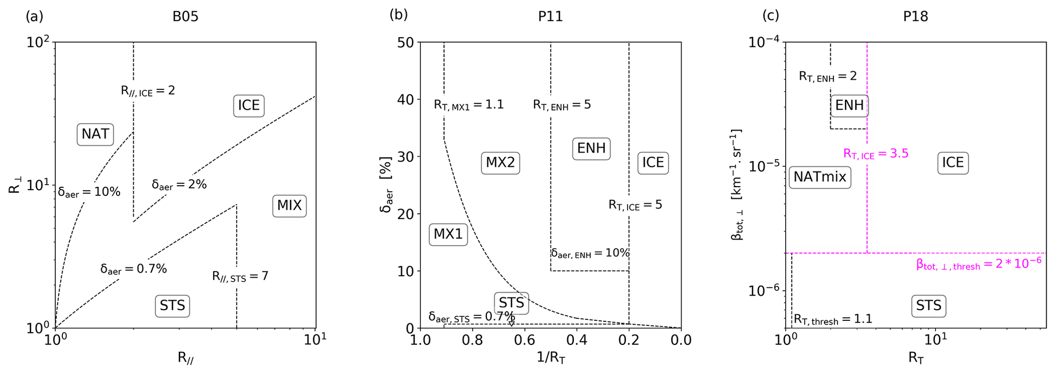
Figure 2 The three classification schemes considered in the paper: B05 (a), P11 (b) and P18 (c). The relevant thresholds are specified. The two dynamic thresholds are coloured in fuchsia and the given values are only for visualization purposes.

B05 is based on the measurements of the ground-based lidar located at Esrange, Sweden, conducted between 1996 and 2004. B05 relies on R_∥, R_⟂ and δ_aer, the latter being related to R_∥ and R_⟂ via Eq. (4). This classification sorts PSC measurements into NAT, STS, ICE and MIX, the latter being a mixed-type one. The threshold separating PSC layers from background aerosols in B05 is $R_{\parallel ,\mathrm{thresh}}=\mathrm{1.06}$. As for the reference properties, NAT clouds are composed of non-spherical crystals and thus exhibit an important depolarization ratio (δ_aer>10 %) and low parallel backscatter ratio ($R_{\parallel }<\mathrm{2}$). STS PSC are spherical liquid droplets theoretically producing no depolarization and a moderate parallel backscatter ratio ($R_{\parallel }<\mathrm{5}$). ICE clouds, due to being dominated by large ice crystals close to the granulometry of cirrus clouds, are associated with depolarization ratios most often largely above 2 % and R_∥ between 2 and 7, or only R_T>7. The MIX class theoretically gathers all PSC measurements not fitting the three previously introduced types: they cover several different physical or chemical states. B05 types and thresholds are summed up in Fig. 2a.

P11 is based on lidar satellite measurements from CALIOP. This scheme relies on R_T and δ_aer. While P11 uses these two variables to sort the PSC types it is worth mentioning that R_T and ${\mathit{\beta }}_{\mathrm{tot},⟂}$ are used to detect PSC layers from the lidar profiles. P11 lists five different types: STS, ICE, NAT-Mix1 (MIX1), NAT-Mix2 (MIX2) and Mixed-enhanced (ENH). ENH particles are most often related to the orographic features that are not expected to be frequent above DDU (Tsias et al., 1999). STS and ICE correspond to the same definitions as in B05, even if the variables used and the corresponding thresholds change. However, the B05 MIX category does not correspond to the mixed categories involved here. P11 types and thresholds are summed up in Fig. 2b. Two thresholds are not specified in Fig. 2b: the δ_aer threshold between ICE and STS, which is a boundary decreasing linearly from ${\mathit{\delta }}_{\mathrm{aer},\mathrm{STS}}=\mathrm{0.7}$ % to 0 % as R_T increases. The separation between MIX1 and MIX2 is thoroughly described in Pitts et al. (2009) and comes from optical calculations. This boundary sorts PSCs according to their NAT number density or volume: clouds with low NAT number density or low NAT volume will most likely be MIX1 while high NAT number density or high NAT volume will be sorted as MIX2 (Pitts et al., 2009).

Using spaceborne lidar measurements, a lower signal-to-noise ratio as compared to ground-based measurements is expected, counterbalanced by the sheer amount of profiles acquired over time, once again compared to the ground-based setup. Horizontal averaging as well as a short time integration also contribute to increase noise significance for spaceborne measurements. This is the reason why, following the recommendation of Achtert and Tesche (2014), some thresholds used in P11 should be adapted when applied to ground-based measurements. The adapted thresholds are shown in Fig. 2b. The R_T threshold between background and PSC layers is lowered from 1.25 to 1.1. While Achtert and Tesche (2014) advocates the use of ${\mathit{\delta }}_{\mathrm{aer},\mathrm{STS}}=\mathrm{0.4}$ % for the STS upper limit of depolarization, we set it to ${\mathit{\delta }}_{\mathrm{aer},\mathrm{STS}}=\mathrm{0.7}$ % in order to be consistent with B05, also considering it is a ground-based setup. P11 original value was ${\mathit{\delta }}_{\mathrm{aer},\mathrm{STS}}=\mathrm{3.5}$ %.

P18 is also based on CALIOP and is the update of P11. It still relies on R_T but now considers ${\mathit{\beta }}_{\mathrm{tot},⟂}$ instead of δ_aer. As mentioned previously, P11 already used ${\mathit{\beta }}_{\mathrm{tot},⟂}$ for layers detection. P18 still features STS, ICE and ENH types, but P11 types MIX1 and MIX2 have been merged in a single category, NAT-mixtures (NATmix). The main update between P11 and P18 is that the latter includes three dynamically computed thresholds. Instead of having fixed values, they depend on the uncertainty of each measurement or on the abundance of relevant atmospheric species, H₂O and HNO₃. Such dynamic thresholds are well-adapted to a spaceborne lidar which experiences various atmospheric conditions. The three thresholds concerned are R_T,thresh, ${\mathit{\beta }}_{\mathrm{tot},⟂,\mathrm{STS}}$ and R_T,ICE. P18 types and thresholds are summed up in Fig. 2c.

In P18, measurement uncertainties are computed with CALIOP-based methods (Liu et al., 2006; Hostetler et al., 2006). When adapting P18 to DDU lidar measurements, we somewhat simplified the dynamic thresholds: R_T,thresh, the R_T boundary separating background measurements from PSC layers was fixed at $R_{T,\mathrm{thresh}}=\mathrm{1.1}$ as in P11, following the conclusion of Achtert and Tesche (2014). The threshold ${\mathit{\beta }}_{\mathrm{tot},⟂,\mathrm{STS}}$ separating STS droplets or aerosols from NAT particles and ICE crystals was also fixed but with a dependence on altitude. The ${\mathit{\beta }}_{\mathrm{tot},⟂,\mathrm{thresh}}$ profile was defined as mean + 1 standard deviation of all ${\mathit{\beta }}_{\mathrm{tot},⟂}$ values corresponding to background and STS measurements at DDU, per 1 km vertical interval. To do so, B05 and P11 classifications were used. The ${\mathit{\beta }}_{\mathrm{tot},⟂,\mathrm{thresh}}$ profile, not shown here, displays a strong altitude dependency: in the stratospheric range of PSC occurrences, the threshold variation range spans two orders or magnitude.

In P18, the R_T,ICE value separating NAT mixtures and ENH from ICE is calculated from the nearly coincident H₂O and HNO₃ Microwave Limb Sounder (MLS) measurements, Aura and CALIPSO satellites being both on the A-train constellation. From H₂O and HNO₃ total abundances, theoretical calculations of R_T lead to a dynamic R_T,ICE threshold. The change of R_T NAT/ICE limitation between P11 and P18 is significant: from $R_{T,\mathrm{ICE}}=\mathrm{5}$ in P11 to R_T,ICE in [2.75–4] in P18. Such a change has direct impact on classification outcomes. We choose to use the R_T,ICE values provided by CALIOP in the PSC Mask v2 product. For each DDU lidar measurement, the R_T,ICE value was taken from the closest CALIOP profile in time and space in the 100 km radius area around the station.

The wave–ice category defined in P11 and P18 (R_T>50) was ignored since it is not relevant above DDU. ICE PSC induced by orographic gravity waves are very unlikely to be observed at DDU due to its location, and it indeed was never detected.

Most of the published classifications, including B05 and P18, feature a mixed-type category. Mixed-type clouds may actually describe different physical realities: a MIX cloud type layer may actually be a fine stack of chemically different layers (finer than the instrumental final vertical resolution of the classification algorithm) or it can also be the signature of particles outside the thermodynamical equilibrium and actually be evolving along with temperature. The lidar geometry is such that only a small atmospheric air column is probed above the instrument and therefore high variability is expected at stratospheric altitudes with the speed of air masses and different equilibration times for PSC particle population. These non-equilibrium particles therefore need to be classified, and it is thus expected that they represent a significant part of observations, regardless of the classification scheme.

4 Results

4.1 Two-variable classification

Before discussing the distributions of PSC types at DDU according to B05, P11 and P18 classification schemes, we provide statistics on CALIOP PSC detections around DDU using the method described in the previous section and inspired by Snels et al. (2021). The Concordia station, focus of the Snels et al. (2021) study, is located 1000 km deeper into the Antarctic continent, whereas DDU has a littoral position and is often located at the edge of the polar vortex. As a result, PSC observations at DDU are lower than at Concordia. Within a distance of about 100 km around Concordia from 2014 to 2018 and from June to September, Snels et al. (2021) finds 369 available CALIOP orbits, 88 of which do not include any PSC. From 2007 to 2020, using the same criteria, only 392 orbits are found around DDU, 299 of which do not include any PSC. This highlights the small number of CALIOP orbits available in the domain around DDU, as was also pointed out by Tesche et al. (2021, Fig. 8). Among these orbits, the proportion of PSC is also significantly lower at DDU than at Concordia. This is illustrated by Fig. 7 of Tesche et al. (2021) who identify 74115 vertical bins in a 4^∘ × 4^∘ domain around Concordia and only 7056 around DDU, based on the Antarctic winters of 2012 and 2015. This is a reminder of the marginal position of DDU with respect to the polar vortex and highlights the difficulty of comparing measurements acquired in this area with those from CALIOP due to the small number of compatible measurements.

The PSC types distribution resulting from the application of DDU PSC measurements using B05, P11 and P18 schemes are shown in Fig. 3. The distribution of PSC types at DDU based on CALIOP measurements and P18 scheme is also included in Fig. 3d. To make the comparison valid, we restricted our analysis to the months of June, July, August and September. Figure 3 globally shows a very good agreement between the studied classification schemes. First, the STS abundance is in very good agreement in all cases: between 27.4 % and 35.4 %. In order to compare the abundance of NAT and NAT mixtures in each classification, the relative abundance of NAT and mixed categories was summed for each scheme, as proper comparison needs to account for the differences in the schemes. For B05, NAT + MIX types weight 64.4 %. For P11, MIX1 + MIX2 + ENH types account for 70.7 % of all PSC types. For the distributions based on P18, NATmix + ENH categories make up for 61 % and 62.1 % of the total for the datasets based on DDU lidar and CALIOP measurements respectively. These small differences reflect the discrepancies between the ICE proportions in all schemes.

Figure 3 PSC types distribution observed at DDU for the three considered classifications: B05 (a), P18 (b), P11 (c) and observed by CALIOP extracted around DDU using P18 scheme (d).

The ICE abundance presents an important variability among the four diagrams. The first reason for this variability comes directly from the thresholds considered: as it was previously highlighted, the evolution of R_T,ICE from P11 to P18 is significant and explains an important discrepancy between the resulting ICE percentages. B05 classifies a PSC as ICE if δ_aer>2 % and R_∥ in [2, 7], or if R_T>7. Furthermore, the actual definition of R_T as $\frac{R_{\parallel }+R_{⟂}\times {\mathit{\delta }}_{\mathrm{mol}}}{\mathrm{1}+{\mathit{\delta }}_{\mathrm{mol}}}$ considering a very low δ_mol=0.00443 leads to clear dominance of R_∥ in R_T. Consequently, the ICE definition in B05 is more permissive than in P11 and P18 to a lesser extent: some PSCs are classified as ICE in B05 while they are considered as NAT in P11 and P18, which is consistent with the differences observed in Fig. 3.

The PSC types distribution based on CALIOP measurements around DDU and P18 scheme displays 9.9 % of relative abundance for the ICE type. As this is based on P18, the previous remark on the role of the ICE threshold in P18 still applies here. However, the ICE share in Fig. 3d is still higher than in Fig. 3b. The difference most likely comes from the point of view of both lidars and different operational constraints. CALIOP, being a spaceborne lidar, directly accesses the stratosphere whereas a ground-based instrument sounds the troposphere before reaching it. As for our system, and for instrumental safety concerns, the system is not operated in case of thick tropospheric cloud cover. In fact, studies in the Arctic and the Antarctic suggest a correlation between tropospheric cloudiness and ICE PSC occurrences (Achtert et al., 2012; Adhikari et al., 2010). Overall, the presence of thick tropospheric clouds is thought to help in reaching PSC-enabling stratospheric temperatures. This reasoning plainly explains the lesser ICE observations above DDU from the ground as compared to CALIOP. Between 2007 and 2020, CALIOP detected ICE PSC above DDU on 19 different days, out of which 4 correspond to DDU measurements, suggesting a possible important tropospheric cover or bad weather condition hindering operations. However, we do not consider this small sample robust enough to support the analysis. Still, ICE PSC occurrences are expected to remain marginal among PSC observations at DDU as the station is located at the edge of the polar vortex and far from orographic gravity wave sources. This small ICE abundance at DDU is supported by Pitts et al. (2018).

At McMurdo Antarctic station (77.85^∘ S, 166.66^∘ E), from 2006 to 2010, Snels et al. (2019) reported a mean distribution of 13.8 % STS, 71.6 % NATmix, 2.6 % ENH and 12 % ICE. During this period, CALIOP observed approximately 10 % more STS and 10 % less NATmix and otherwise shows a good overall agreement with the ground-based lidar. Snels et al. (2021) compare Concordia ground-based PSC detections to CALIOP measurements around the station from 2014 to 2018. This study mainly focuses on the agreement between ground-based and spaceborne instruments and does not directly provide the PSC type distribution observed at Concordia by the local lidar but still shows the distribution observed by CALIOP around the station. From 2014 to 2018, the yearly occurrences of STS represent from 14 % to 38 %, NATmix from 42 % to 67 %, ENH from 5 % to 11 % and ICE from 10 % to 28 %. The distribution shows a high annual variability, but we still can point out differences with DDU PSC types distribution. Both McMurdo and Concordia measurements feature a higher proportion of ICE detections and less STS observations as compared to DDU. The 38 % STS share observed at Concordia in 2014 is considered to be an outlier. This is consistent with the results of Fig. 19 of Pitts et al. (2018) which show that main area of ICE occurrence is located inside the continent while DDU is located on the Antarctic coast. The temperature necessary to form ICE crystals is reached less often at DDU, on the edge of the vortex.

Figure 4 Distribution of the PSC measurements acquired at DDU between 2007 and 2020 based on the three classification schemes considered: B05 (a), P11 (b) and P18 (c). The number of points per bin is colour-coded and each plot is based on a 5 × 50 bins grid.

The distribution of DDU PSC measurements in B05, P11 and P18 classifications is shown in Fig. 4 and presents where the measurements are concentrated, providing another point of view on the classification thresholds. In Fig. 4a and b, it is worth noting that the distribution displays an increase slightly below the STS depolarization threshold. For B05, the absence of measurements along the bottom x axis is most likely the sign of a small crosstalk noise. Then, it appears that most of the measurements are classified as MIX in B05. This is consistent with Fig. 5b from Achtert and Tesche (2014) which also exhibits high densities in the MIX classes. Given the 10 % depolarization threshold and the relatively low amount of NAT clouds identified by B05, we consider that B05 classifies as NAT the PSCs that are only composed of, or highly dominated by, NAT particles. Whereas P11 and P18 separate NAT mixtures into MIX1, MIX2 and NATmix which may include a significant share of STS droplets.

As for ICE clouds, B05 characterizes significantly more ICE measurements as compared to P11 and P18, where they remain marginal. The relatively low number of ICE events we report relates to the fact that ICE PSC fields above DDU are more unstable than those remaining deep inside the vortex. The optical properties of the ICE clouds observed at DDU are thus expected to be closer to the respective boundaries of the scheme, and this overall lead to greater variability in characterization among the different schemes. As an illustration, we take the PSC event detected on 11 July 2011 with a depolarization ratio of 3.6 % and a total backscatter ratio of 2.3 ($R_{\parallel }=\mathrm{2.034}$ and $R_{⟂}=\mathrm{9.43}$). B05 classifies it as ICE while P11 and P18 classify it as MIX1 and NATmix respectively. From Fig. 4b and c, we conclude that the ENH class is marginal at DDU and is rarely detected. Still, CALIOP classifies 7.1 % of the PSC detections around DDU as ENH. This is likely due to higher ${\mathit{\beta }}_{\mathrm{tot},⟂}$ values measured by CALIOP than by DDU lidar or to a difference in the ${\mathit{\beta }}_{\mathrm{tot},⟂,\mathrm{thresh}}$ threshold used, as Fig. 4c shows it.

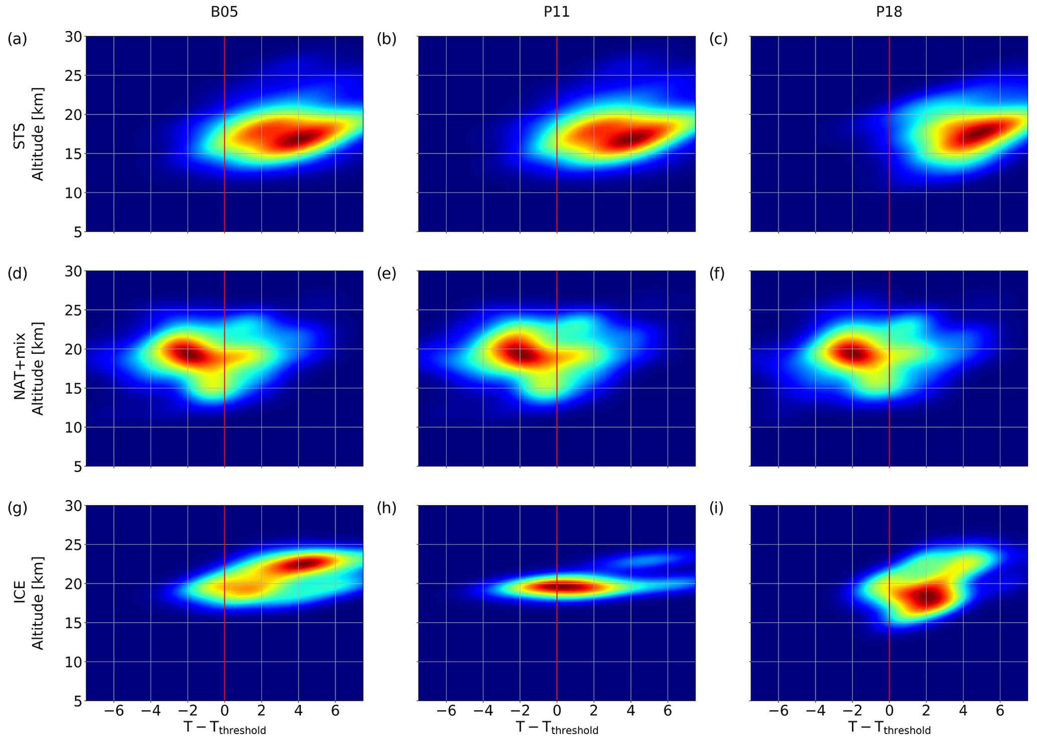
Figure 5 Distribution of PSC detection at DDU from 2007 to 2020 as a function of altitude and temperature relative to the relevant thresholds T_STS, T_NAT and T_ICE. Lines correspond to STS (a–c), NAT + mixtures (d–f) and ICE (g–i). Columns correspond to the classification schemes B05 (a, d, g), P11 (b, e, h) and P18 (c, f, i).

The distribution of PSC layers as a function of temperature and altitude was computed for B05, P11 and P18 for STS, NAT + mix and ICE clouds. The category NAT + mix gathers all types related to NAT particles or mixed categories, i.e. NAT + MIX for B05, MIX1 + MIX2 + ENH for P11 and NATmix for P18, as it is the best way to compare B05, P11 and P18 outcomes. The distributions were computed using kernel density estimation, also referred to as Parzen–Rosenblatt method, a non-parametric method used to estimate probability density functions of a given sample (Rosenblatt, 1956; Parzen, 1962). The distributions for each classification scheme and PSC type are shown in Fig. 5.

For each PSC measurement, MLS H₂O and HNO₃ concentrations are used to compute the relevant threshold temperatures. These temperatures are called T_NAT, T_STS and T_ICE hereafter. T_STS relates to a change in the composition of the aerosols and we considered a 50 % volume mixing ratio of HNO₃ in the condensed phase. Figure 5 presents the distribution of PSC measurements as a function of altitude and temperature relative to the relevant type threshold.

Temperature is not a variable in our PSC detection method, yet we note that most NAT + mix measurements are below the T_NAT threshold within expected uncertainties related to MLS and ERA5 data. Considering STS, it appears that temperatures are above the threshold for all schemes. This is partly expected as T_STS is not associated with a discrete physical phase transition but with a continuous chemical composition change within the droplet. Finally Fig. 5 highlights again that the major difference among classification schemes concerns the ICE category as the three patterns of Fig. 5g, h and i show very different shapes. It is important to read the ICE related plots with caution as the densities are computed from a reduced number of points. It appears however that P11 classifies few PSCs as ICE but those are in the adequate temperature range while B05 and P18 sort most of the ICE PSCs above T_ICE.

Figure 5 also shows that the different types have slightly different altitude domains. All classifications agree in that STSs mostly form between 15 and 20 km, while ICE are usually detected around the average 20 km altitude. NAT + mix category occupies a wider domain, from 15 to 25 km. Since this category includes mixtures, it is not surprising that its range is actually wider. As a reminder B05 defines the MIX category as any measurement not belonging to any of the other classes.

Finally, temperature values associated with PSC types gathered in Fig. 5 are derived from ERA5 reanalyses and are relevant for the intercomparison of the classification schemes, but they may not resolve small-scale variations or features that are important for PSC formations pathways. Also, the time of lidar PSC measurement does not exactly match ERA5 data and MLS H₂O and HNO₃ measurements, which necessarily generates uncertainty. The relevancy of ERA5 reanalyses in the study of PSC at DDU is reviewed in Sect. 4.3.

4.2 Sample PSC event of interest: 28 August 2015

Figure 5 showed that B05, P11 and P18 have comparable outcomes. The most recent scheme (P18), which also features the least amount of classes, was therefore selected to report a DDU PSC event as an illustration of the detection methodology. The lidar time series is presented in Fig. 6a. At the cost of a reduced SNR implied by the 15 min time integration, the short-scale dynamics of the PSC layers are visible. The signal is horizontally smoothed on a 30 min window. The measurements shown in Fig. 6 are obtained on 28 August 2015 from 10:05 until 20:20 UTC. As elements of context, we present in Fig. A1 the outputs of a chemistry–transport model available in the institute (REPROBUS coupled to the MIMOSA transport scheme), resolving PSC formation from the thermodynamical equilibrium assumption and a modal size scheme for the microphysics, accounting for temperature tracers of time elapsed below T_NAT and T_ICE. References on the transport model can be found in Hauchecorne et al. (2002) and on the chemistry module in Lefèvre et al. (1994). Figure A1 shows PSC flag presence at the 435, 475 and 550 K potential temperature levels computed from ERA5 reanalyses. The model produces PSC presence at the 435 and 475 K levels and no PSC at the 550 K level above DDU, which is consistent with the lidar measurements.

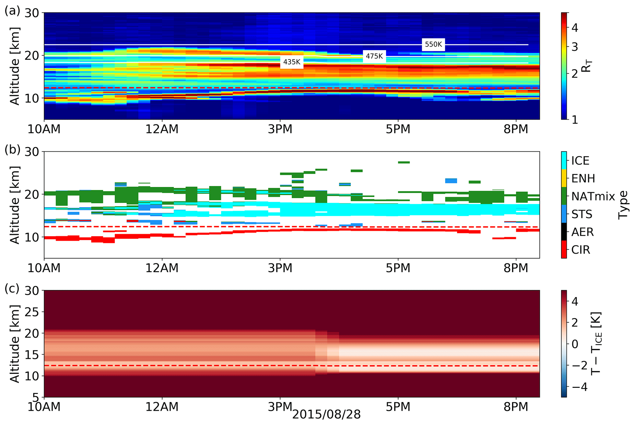
Figure 6 The 532 nm backscatter ratio of lidar measurements obtained at DDU on 28 August 2015 (a). The corresponding PSC types according to P18 classification scheme (b) and ERA5 temperatures at DDU as compared to the ICE formation threshold T_ICE, calculated from the MLS H₂O of the day (c). The red dashed line indicates the dynamic tropopause computed from ERA5 data.

Figure 6a also highlights the high temporal variability of PSC layers at the DDU latitude. This high variability must be kept in mind as well as the trade-off on the integration time between SNR and information loss caused by the averaging of potential varying atmospheric scenes due to the air masses transport. Figure 6 also underlines the contrast between the reality of a complex shape of the 3D PSC field and the necessary and legitimate stance of recent classification schemes to keep things as simple as possible. PSCs are evolving depending on their stratospheric environment. While PSC particles are constantly growing or shrinking, taking up H₂O or HNO₃ from the gas phase or enriching it, the classification schemes keep up with fixed thresholds as temperature history has not been accounted for. On Fig. 6b, the type identified for the PSCs located at 20 km changes several times from NATmix to ICE. Since this measurement is processed with P18, it implies that R_T has just crossed the R_T,ICE threshold. The PSC chemical composition may not have changed, but its optical properties may have shifted it from one class to another.

Figure 6a and b also illustrate the stack of fine PSC layers, it is especially clear between 10:00 and 15:00 UTC. In the beginning of the measurement session, some of the layers at the bottom of the stratosphere are interpreted as STSs while the upper ones are classified as NATmix. Then, starting from noon and until the end of the session, R_T increases and the PSC becomes ice dominated. This evolution is consistent with the ERA5 temperatures shown in Fig. 6c. In the first half of the session the temperature of the domain between 10 and 18 km is slightly above T_ICE but then reaches this threshold on a thinner domain in agreement with the lidar PSC detection of Fig. 6a and b which layer becomes thinner as time elapses during the day.

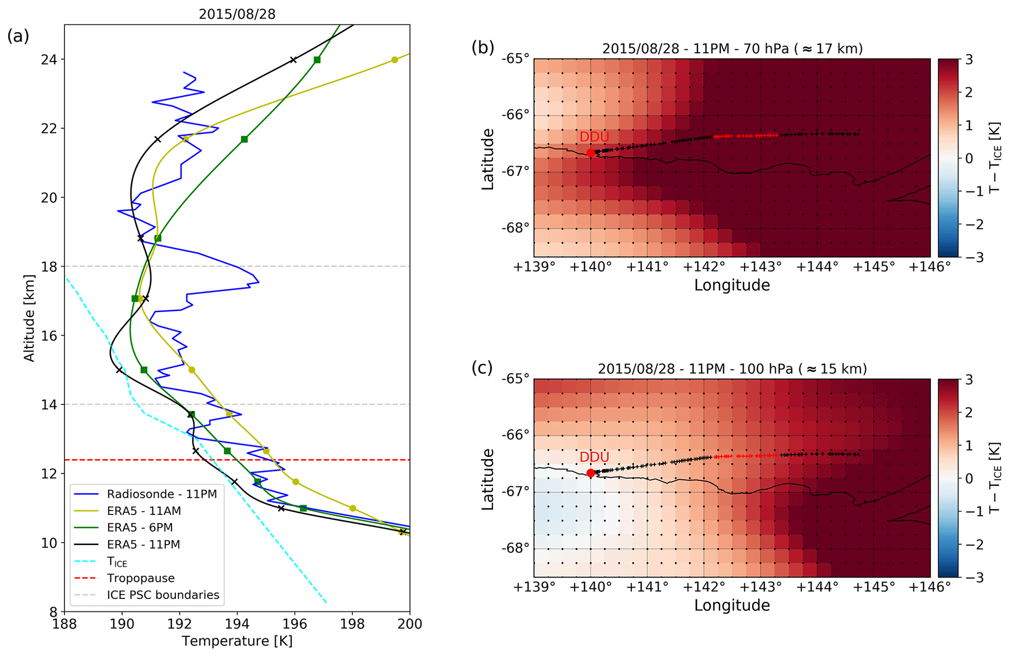
Figure 7 (a) 28 August 2015 DDU temperature profiles from a local radiosonde launched at 23:00 UTC (blue line), ERA5 reanalyses at 12:00 UTC​​​​​​​ (green line), at 18:00 UTC (yellow line) and at 23:00 UTC (black line). T_ICE threshold temperature is indicated by the sky blue dashed line; the red dashed line shows the dynamic tropopause from ERA5. The boundaries of the ICE PSC detected at DDU from approximately 15:00 to 20:00 UTC are shown by grey dashed lines. (b, c) Temperature fields from ERA5 reanalyses on 28 August 2015 at 23:00 UTC respectively at 70 hPa, approx. 17 km, and 100 hPa, approx. 15 km. The trajectory of the radiosonde launched at DDU on 28 August 2015 at 23:00 UTC is shown by black and red dots. Red dots correspond to heights between 14 and 18 km i.e. the boundaries of the ICE PSC detected at DDU.

To further check the temperature evolution regarding T_ICE, Fig. 7a compares T_ICE (sky blue dashed line) to ERA5 temperatures profiles at 11:00, 18:00 and 23:00 UTC (yellow, green and black lines respectively). The ERA5 profile at 23:00 UTC is included in order to be compared to the radiosonde temperature launched at DDU at 23:00 UTC (blue line). The discrepancies between ERA5 and DDU radiosonde temperatures are actually associated with the drift of the radiosonde as its altitude increases. Figure 7b and c show ERA5 T−T_ICE fields around DDU at 23:00 UTC at 70 and 100 hPa (approximately 15 and 17 km respectively) together with the trajectory of DDU radiosonde (black and red dots). Red dots show the location of the radiosonde between 14 and 18 km, i.e. the boundaries of the ICE PSC detected at DDU. This one example highlights the recurrent drift of the radiosonde leading to use of reanalyses for climatological purposes. While ERA5 temperature between 14 and 18 km at DDU are compatible with an ICE PSC, the radiosonde tells a different story. Radiosonde drift is closely connected to temperature uncertainties, and we discuss this point in the next section, as temperature is a critical variable in threshold processes like cloud formation.

4.3 Temperature datasets

Lidar data processing heavily relies on accurate temperature data due to Rayleigh scattering and extinction correction to get the Mie contribution out of the raw signal. PSC characterization is also closely connected to temperature thresholds, as shown in Figs. 6 and 7. In that regard, the choice of temperature dataset should be done with caution. In order to use the most adapted temperature dataset to process our PSC measurements at DDU, we compare several ones in Fig. 8, from reanalysis to satellite observations. Figure 8a shows the distribution of DDU radiosondes locations between 15 and 25 km, i.e. the stratospheric altitude range of most PSC occurrences, from 2010 to 2020 (radiosondes were not equipped with a GPS before 2010). Figure 8b, c and d present the temperature difference between ERA5 (Fig. 8b – ΔT_ERA5−RS), NCEP (Fig. 8c – ΔT_NCEP−RS) and IASI (Fig. 8d – ΔT_IASI−RS) with respect to DDU radiosondes from June to September, from 2007 to 2020. The IASI temperature product provides high spatial resolution and daily temperature profiles included in a narrow box of 0.6^∘ longitude width and 0.3^∘ latitude height centred on DDU from 2008 onwards. The area used to extract IASI temperature profiles is delimited by a red dashed rectangle in Fig. 8a.

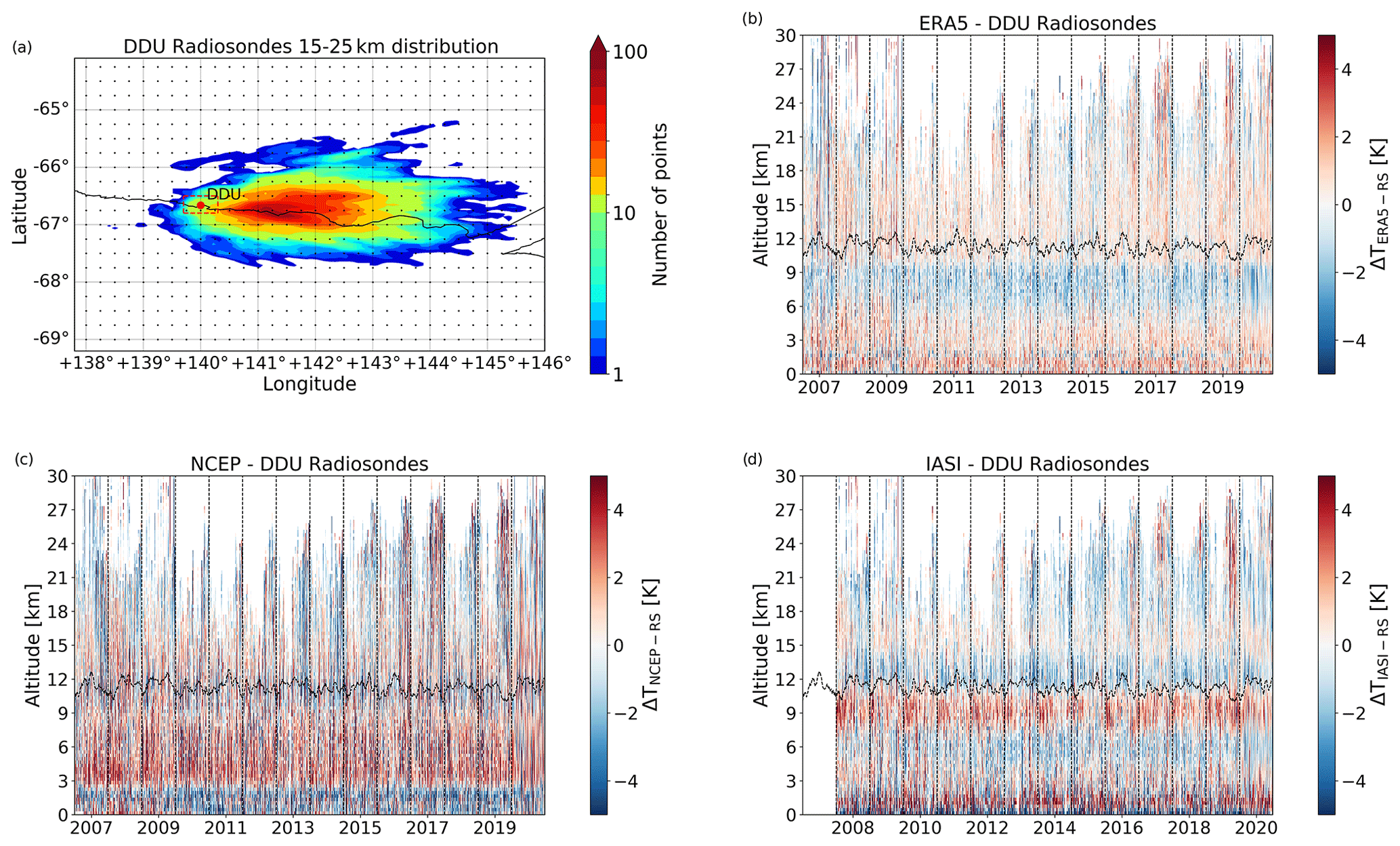
Figure 8 Spatial distribution of radiosonde measurements between 15 and 25 km from June to September from 2010 to 2020 (a). The number of points per bin is colour-coded; the grid size is 100 × 100 bins. Black dots indicate the ERA5 grid. The red dashed rectangle delimits the area used to extract IASI temperature profiles. Difference between temperature given by ERA5 (b), NCEP (c) and measured by IASI (d) as compared to radiosondes launched at DDU from June to September from 2007 to 2020. The black dashed line indicates the dynamic tropopause based on ERA5.

Temperature profiles from DDU radiosondes were not retained for this climatological study for two reasons. First, they are launched at DDU every day around 09:00 local time, and the lidar is operated at nighttime, so a discrepancy might arise, especially during summer. Second, as it can be inferred from Fig. 8b, c and d, radiosondes often burst reaching between 15 and 25 km in the wintertime (see Fig. A2 in Appendix) and therefore do not provide the full temperature vertical profile. Figure 8a highlights this important horizontal transport. Figure A2 in the Appendix shows the distribution of the distance to DDU at which radiosondes burst, from 2010 to 2020, in summer and in winter. To illustrate that such horizontal transport can have significant impact on the temperature retrieved by radiosondes as compared to the stratospheric conditions above DDU, Fig. A3 in the Appendix presents six examples of ERA5 temperature fields over the same geographical areas as Fig. 8a. These examples show the variety of spatial temperature patterns experienced around DDU and emphasize that radiosondes should be used with caution as this important horizontal transport is often not taken into account. At least during polar winter, temperature profiles retrieved from radiosondes should not be considered as purely representative of the launch pad location.

We basically consider three temperature datasets, two are reanalyses, ERA5 and NCEP, and the third one is an inversion product out of IASI satellite radiances. Figure 8b, c and d present an intercomparison with radiosondes launched at DDU from June to September, from 2007 to 2020. First, NCEP is obviously less accurate that ERA5 and IASI, both in the troposphere and in the stratosphere. The difference between ERA5 and IASI seems not to be significant and the comparison with radiosondes exhibits altitude-dependent patterns. For ERA5, ΔT_ERA5−RS is positive in the stratosphere and negative in the upper troposphere. For IASI, a positive ΔT_IASI−RS bias is recorded below the tropopause suggesting a difficulty in assessing the tropopause height, or a vertical resolution problem (the IASI dataset is a 11-layer product between 750 and 7 hPa, whereas ERA5 has a finer resolution). To quantify the deviation of ERA5, NCEP and IASI with respect to the radiosondes, the standard deviation of ΔT_ERA5−RS, ΔT_NCEP−RS and ΔT_IASI−RS was computed between 15 and 25 km. It reaches 1.0 K for ERA5, 2.0 K for NCEP and 1.1 K for IASI. Considering the above statements, and the finer vertical resolution of the ERA5 temperature product, we consider the use of the ERA5 temperature the most relevant to our study.

4.4 PSC trend estimation

As mentioned in introduction, ground stations are key to the establishment of decadal trends. Operating instruments at high latitudes for decades remains a technical and logistical challenge, and the focus is put on continuous monitoring. Bad weather or thick tropospheric cloud cover hinders the operation of the lidar. Therefore, comparing the raw number of PSC days per year would be strongly biased by the number of days on which the lidar is effectively operated each year. The statistics of operations is the critical point in establishing a trend here, see Fig. 1. We choose to complement the statistics of lidar measurements with a temperature proxy, considering that PSCs form when temperature drops below T_NAT. For qualitative and counting purposes, this assumption is fully valid and will be illustrated hereafter. ERA5, NCEP and IASI temperatures are used to compile stratospheric temperature above DDU. Using these temperatures, a number of potential PSC days is computed, i.e. the number of days where PSCs could occur based only on temperature. The number of PSC days per year is the variable considered in order to circumvent the challenging issue of delimiting PSCs both in time and space.

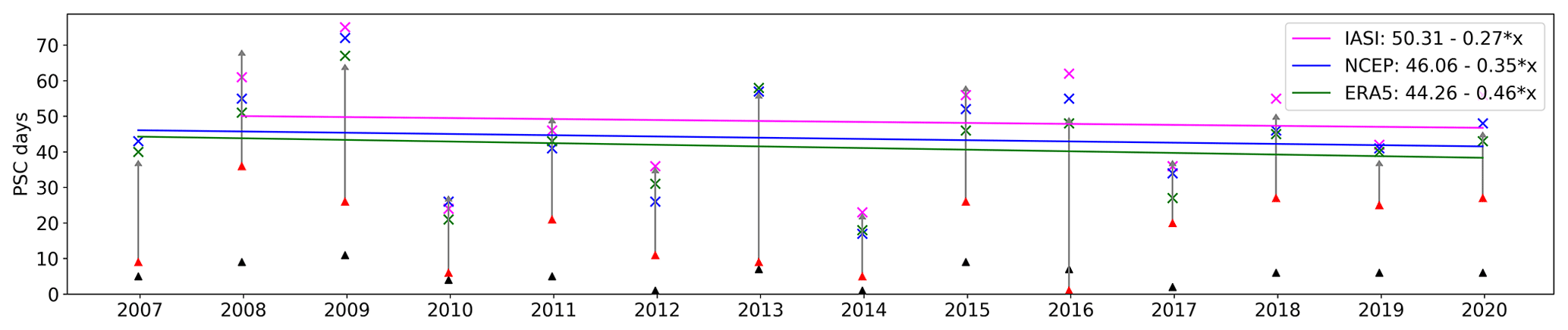
Figure 9 PSC days per year at DDU from 2007 to 2020 featuring PSC detection with the DDU lidar in red triangles and with CALIOP in black triangles. Potential PSC days per year estimated by ERA5, NCEP and IASI based on the lidar measurements are shown with green, blue and fuchsia crosses respectively. Green, blue and fuchsia lines represent the corresponding trends. Grey arrows indicate the number of days per year where the $T-T_{\mathrm{NAT}}<-\mathrm{1}$ K criterion was satisfied and the DDU lidar was not operated.

Mainly due to chemical kinetic concerns, PSCs generally form a few degrees below T_NAT (Dye et al., 1992). Using the condition $T-T_{\mathrm{NAT}}<\mathrm{0}$ to state if a day is a potential PSC day could then lead to an overestimation of the number of PSCs. In order to refine the criterion, we computed for each year the number of days satisfying the condition $T-T_{\mathrm{NAT}}<\mathrm{\Delta }T$ per year, with ΔT ranging from 0 to −10 K on the days lidar measurements were available. The results obtained with the different ΔT values were compared with the number of PSC days detected by the lidar. The result lead to a similar value for ERA5, NCEP and IASI of $\mathrm{\Delta }T=-\mathrm{1}$ K. Figure 9 shows the 2007–2020 PSC days per year built on ERA5 (green line), NCEP (blue line) and IASI (fuchsia line) based on this criteria, as well as the number of PSC days detected by the lidar with red triangles. The grey arrows indicate the number of days per year satisfying the $T-T_{\mathrm{NAT}}<-\mathrm{1}$ K criteria with no coincident lidar measurements. The T_NAT values have been computed based on the daily MLS H₂O and HNO₃ measurements at DDU.

The number of PSCs detected by the lidar in Fig. 9 is consistently and logically below the one estimated by the temperature datasets. The three datasets were considered for the trend calculation to show that despite the discrepancies they all indicate an approximately similar trend. From Fig. 9, we note a decreasing trend of −4.6 PSC days per decade that could not have been inferred from the lidar measurements alone. The 14-year trend remains significant when its sensitivity is tested regarding the ΔT criterion or the impact of any single year. Given the temperature-based criterion used, this trend means that the temperature of the stratosphere above DDU is experiencing an opposite trend, as PSC occurrences directly correlate to temperature changes.

Temperature trends computed with IASI over the 2008–2020 period show significant warming above Dumont d'Urville (0.1 K yr⁻¹ between 200 and 70 hPa, adapted from Bouillon et al. (2022), shown in Fig. A4). ERA5 trends over the same period show very similar results. As mentioned in Tritscher et al. (2021), the acceleration of the Brewer–Dobson circulation linked to climate change counteracts the expected cooling from greenhouse gases at high latitudes. The recovery of the ozone hole also advocates for a rise of polar stratospheric temperatures (WMO, 2018). Despite Bouillon et al. (2022) indicating a warming trend that is not specific to DDU, it should be noted that a trend in the size or location of the polar vortex could also contribute to the temperature trend observed at DDU, it is however not the scope of the present study.

If this 14-year trend is negative, it is not the case for longer time spans: using the same method over the period 1992–2020, we conclude on no significant trend. This is consistent with recent studies concluding on no significant trend of PSC occurrences on the continental scale using longer time periods (Tritscher et al., 2021). It is worth noting that David et al. (2010) also established a local temperature trend using 50 years of balloon radiosoundings above DDU, concluding on no significant temperature trend during winter. David et al. (2010) also concluded on a positive but statistically not significant PSC occurrences frequency trend over the period 1989–2008. Similarly, trends computed with ERA5 over 1990–2020 show small or insignificant warming (Bouillon, 2021), which is consistent with the results of others studies where trends were computed on a longer period (Randel et al., 2016; Maycock et al., 2018). This might suggest that the ozone hole recovery has been strengthening in the past decade.

Discussing PSC estimation by models, Tritscher et al. (2021) stated that the PSC volumes derived from ERA-Interim using the T<T_NAT criteria are about 50 % overestimated as compared to the satellite PSC measurements. Such an overestimation may be due to reanalysis uncertainties especially in the calculation of T_NAT. Mostly, this PSC volume evaluation assumes that PSC layers entirely fill the available stratospheric volume satisfying T<T_NAT. This hypothesis does not seem in agreement with our observations at DDU. To check this above DDU, for each day with a PSC detection, we calculated the stratospheric range satisfying the condition T−T_NAT. T_NAT was calculated with the daily MLS H₂O and HNO₃ measurements. Let us call this range H_NAT, expressed in km. We also calculated the geometrical thickness of the PSC detected, called H_PSC. Then, we computed the difference H_NAT−H_PSC: it represents the stratospheric range satisfying T−T_NAT unoccupied by PSC layers. The distribution of this difference for all PSC detections at DDU from 2007 to 2020 is plotted in Fig. 10. Figure 10 tends to show that the stratospheric domain satisfying T<T_NAT is larger than the actual range filled by PSC layers. Given the fact that ERA5 slightly overestimates stratospheric temperature at DDU according to Fig. 8b, the discrepancy between PSC thickness and the stratospheric domain satisfying T<T_NAT could even be underestimated.

Figure 10 Distribution of the thickness of the stratospheric domain satisfying T<T_NAT unoccupied by PSC layers, in km, on days when a PSC is detected at DDU.

5 Conclusions

The stratospheric DDU Rayleigh/Mie/Raman lidar is one of the few instruments monitoring stratospheric aerosol and cloud activity in Antarctica for decades. This study presents PSC measurements acquired from 2007 to 2020. The high vertical and spectral characterization capabilities of lidar instruments remain the best suited to characterize any given particle population, especially at stratospheric altitudes. Optical properties overall shape PSC classifications, which in turn drive the parameterizations of PSCs in models. Over time, many PSC schemes were published using different species, mixtures, optical variables and separation thresholds. In this paper we analyse DDU PSC measurements using three major schemes referred to as B05, P11 and P18; the first relies on ground-based measurements and the other two on CALIOP spaceborne measurements. Laying our measurements on these schemes, a good mutual agreement between all three is established. ICE cloud ratios still vary from one scheme to another, but these differences are directly explained by the design of the classifications. DDU measurements are also compared to a PSC types distribution based on CALIOP PSC measurements around DDU from 2007 to 2020. Ground-based and spaceborne measurements agree relatively well on the types distribution, showing significant disagreement only for the ICE and ENH types, but the relatively low number of CALIOP PSC observations at DDU location explains most of the variability. Connected to this, an established correlation between ICE cloud formation and tropospheric cloud cover should also explain the variability, as it prevents our instrument from operating. The spaceborne geometry always has direct access to the stratosphere without any significant particle extinction. Investigating this correlation is an interesting perspective of this work. Correlating PSC formation temperature to the three chemical classes, ICE clouds are observed at a higher altitude than STS and NAT clouds.

From typical lidar time series, we highlight the small-scale features of PSC layers as well as their temporal variability both in vertical extent and optical properties, discussing time integration influence (both from a ground and space geometry) when using thresholds to characterize cloud types. Smaller local datasets are able to support class definition by refining mesoscale observed behaviours. We also extensively consider the sensitivity of temperature datasets as small-scale proxies for PSC formation thresholds. Overall, we emphasize how the local variability of the measurements acquired at the station closely relates to the dynamics of the vortex and prevalence of horizontal transport at stratospheric altitudes. We compare ERA5 and NCEP reanalyses to a IASI-derived temperature product and to local radiosondes. Related to the coastal location of the station, a significant spatial drift of the sondes during their ascent up to the stratosphere leads us to use temperature reanalyses in lidar data processing to ensure consistency. ERA5 proves to be the most convenient dataset to use locally, showing a satisfying agreement with DDU radiosondes from 2007 to 2020. In the near future, the IASI product should become an interesting option, especially for high latitude sites: the accuracy seems to be the same as ERA5, except in the upper troposphere.

A temperature proxy statistically complements DDU lidar PSC measurement days and we built a 14-year trend of number of PSC days per year. A significant slightly negative (−4.6 PSC days per decade) trend is found between 2007 and 2020 and relates to an opposite trend in term of stratospheric temperatures for southern high latitudes which was also reported in a recent study (Bouillon et al., 2022).

PSC volume is often estimated in models as the stratospheric volume satisfying T<T_NAT, with acknowledged overestimation in derived volumes up to 50 % (Tritscher et al., 2021). DDU lidar measurements show that the PSC detected are often significantly thinner than the stratospheric domain satisfying T<T_NAT. This should have an impact on chemical efficiencies of chemical compound conversion rates involved in stratospheric ozone chemistry, but it is beyond the scope of our paper.

Finally, DDU offers a privileged access to air mass entries into the vortex, which has been studied recently after the 2020 Australian wildfire event above DDU (Tencé et al., 2022). The global impact of volcanic or biomass burning aerosols through long-range transport now attracts more scientific attention, and these events feature, especially after months of transport, optical properties that overlap the one of some PSC types, mainly STS. Speciation between stratospheric sulfate, carbonaceous aerosols and STS PSC type requires extensive measurement capabilities in monitoring stations. Delving into any potential interplay between PSC and aerosol layers also demands consolidated PSC classification schemes.

Appendix A

Figure A1 PSC surface area (µm² cm⁻³) maps from the Reprobus model for 28 August 2015 at 435 K (a), 475 K (b) and 550 K (c). DDU location is indicated by the red dots.

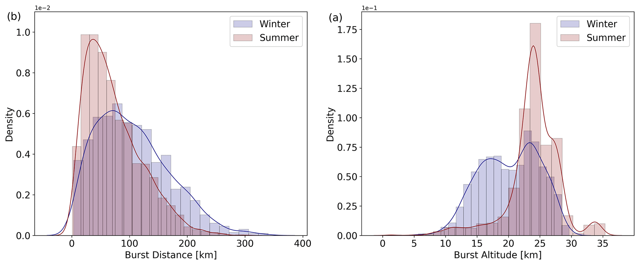
Figure A2 (a) Distribution of the distance between DDU and the burst location of DDU radiosondes in summer (red) and winter (blue) from 2010 to 2020. (b) Distribution of the burst height in summer (red) and winter (blue) from 2010 to 2020. Winter is defined as the period from June to September included, and Summer is the rest of the year.

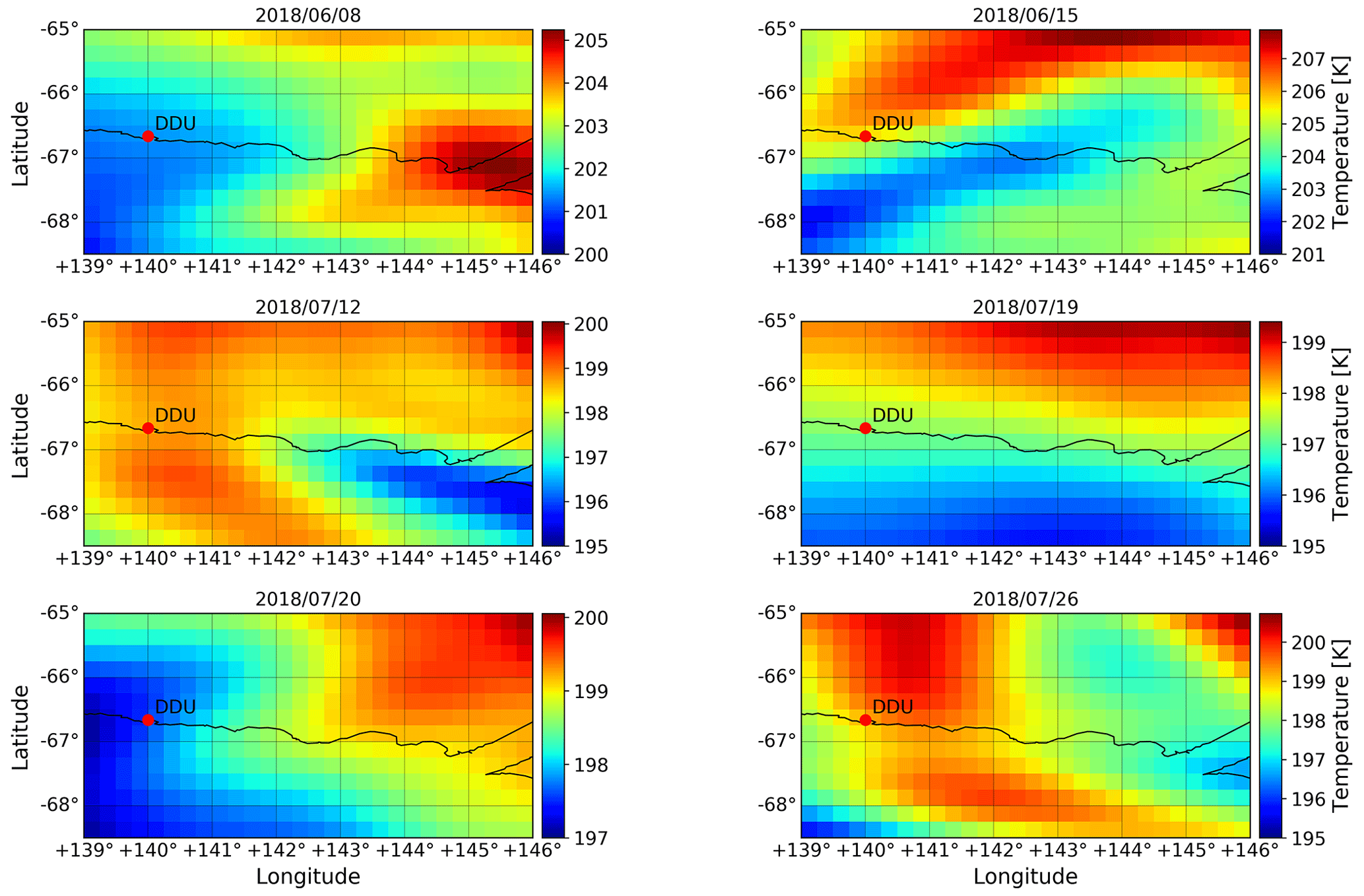
Figure A3 ERA5 reanalyses temperature fields at 100 hPa for the domain corresponding to the radiosondes drift shown in Fig. 8.

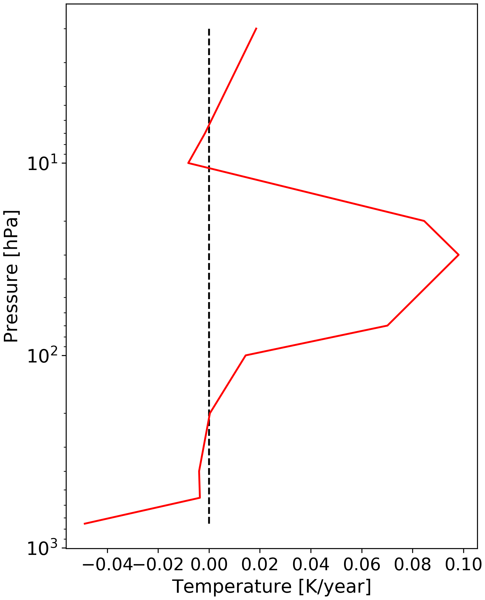
Figure A4 IASI temperature trend at DDU from 2008 to 2020. Adapted from Bouillon et al. (2022).