the Creative Commons Attribution 4.0 License.
the Creative Commons Attribution 4.0 License.
 | 03 Apr 2023
Mean age from observations in the lowermost stratosphere: an improved method and interhemispheric differences
Thomas Wagenhäuser
Markus Jesswein
Timo Keber
Tanja Schuck
Andreas Engel
The age of stratospheric air is a concept commonly used to evaluate transport timescales in atmospheric models. The mean age can be derived from observations of a single long-lived trace gas species with a known tropospheric trend. Commonly, deriving mean age is based on the assumption that all air enters the stratosphere through the tropical (TR) tropopause. However, in the lowermost stratosphere (LMS) close to the extra-tropical (exTR) tropopause, cross-tropopause transport needs to be taken into account. We introduce the new exTR–TR method, which considers exTR input into the stratosphere in addition to TR input. We apply the exTR–TR method to in situ SF6 measurements from three aircraft campaigns (PGS, WISE and SouthTRAC) and compare results to those from the conventional TR-only method. Using the TR-only method, negative mean age values are derived in the LMS close to the tropopause during the WISE campaign in Northern Hemispheric (NH) fall 2017. Using the new exTR–TR method instead, the number and extent of negative mean age values is reduced. With our new exTR–TR method, we are thus able to derive more realistic values of typical transport times in the LMS from in situ SF6 measurements. Absolute differences between both methods range from 0.3 to 0.4 years among the three campaigns. Interhemispheric differences in mean age are found when comparing seasonally overlapping campaign phases from the PGS and the SouthTRAC campaigns. On average, within the lowest 65 K potential temperature above the tropopause, the NH LMS is 0.5±0.3 years older around March 2016 than the Southern Hemispheric (SH) LMS around September 2019. The derived differences between results from the exTR–TR method and the TR-only method, as well as interhemispheric differences, are higher than the sensitivities of the exTR–TR method to parameter uncertainties, which are estimated to be below 0.22 years for all three campaigns.
- Article
(2809 KB) - Full-text XML
-
Supplement
(746 KB) - BibTeX
- EndNote


The lowermost stratosphere (LMS) is the lowest part of the extra-tropical (exTR) stratosphere. Its upper boundary is usually defined as the 380 K isentrope and approximates the lower boundary of the stratosphere in the tropics. The chemical composition of the LMS plays an important role in the climate system. Different transport paths and timescales determine the chemical composition of the LMS for a wide range of trace gases. The most prominent transport mechanism in the stratosphere is the Brewer–Dobson circulation (BDC), which transports air from the tropical (TR) tropopause to the exTR and polar stratosphere (Butchart, 2014). The residual circulation part of the BDC is characterized by two branches (Birner and Bönisch, 2011; Plumb, 2002): one branch extends deep into the middle atmosphere and slowly transports air to high latitudes where it eventually descends to lower altitudes. The shallow branch in the lower part of the stratosphere transports air poleward below the subtropical transport barrier and is characterized by comparably fast transport timescales. In addition to residual transport, air is transported within the stratosphere by bidirectional mixing. Both residual transport and mixing are induced by wave activity on different scales and are part of the BDC. In addition to the BDC, exTR cross-tropopause transport strongly affects the chemical composition of the LMS. This exTR transport mechanism is modulated by the subtropical jet (Gettelman et al., 2011).
The age of air is a widely used concept to describe tracer transport in the stratosphere (Waugh and Hall, 2002). In principle, infinitesimal fluid elements enter the stratosphere across a source region. The transit time (or “age”) of each individual fluid element is the elapsed time since it last made contact with a source region. A macroscopic air parcel in the stratosphere consists of an infinite number of such fluid elements, each with its own transit time. The transit time distribution for the air parcel is called the “age spectrum” (Kida, 1983). Past studies were able to obtain information on age spectra from observations of multiple trace gases (Andrews et al., 1999, 2001; Bönisch et al., 2009; Hauck et al., 2020; Ray et al., 2022). The first moment of the age spectrum is the mean age of air. It can be derived from measurements of a single inert trace gas species with a monotonic trend in the troposphere. CO2, SF6 and a variety of “new” age tracers have been used in past studies to derive the mean age of air from observations (e.g., Engel et al., 2017; Leedham Elvidge et al., 2018).
The age of air from observations provides a stringent test for numerical models. The number of available trace gas observations that are suited to derive mean age is vastly higher than that to derive age spectra. In addition, deriving mean age relies on making fewer assumptions compared to deriving age spectra. This makes mean age a valuable measure to compare models to observations. Still, observational estimates of mean age rely on several simplified assumptions, depending on the trace gas used, which significantly add to the uncertainty in mean age across large areas of the stratosphere. For example, in order to derive mean age from SF6 measurements, an infinite lifetime is commonly assumed. In contrast, recent studies showed that a mesospheric sink of SF6 leads to a significant bias towards higher ages, especially on old mean age values derived from SF6 observations (Leedham Elvidge et al., 2018; Loeffel et al., 2022). Another common assumption is that all air enters the stratosphere through the TR tropopause. However, Hauck et al. (2019, 2020) showed that in the vicinity of the tropopause, transport across the exTR tropopause is also important to adequately describe age spectra and mean age in the LMS. While the assumption of a single entry point is a good approximation for the stratosphere above about 380 K potential temperature θ, this is thus not the case for the LMS. Together with the interhemispheric gradient in tropospheric trace gas mixing ratios, this limits the ability to derive the mean age of air in the LMS. Further improvements of the methods to derive the mean age of air from observations are thus desirable in order to provide robust real world estimates of transport timescales in sensitive regions of the atmosphere and be able to compare them to model results.
With this work we focus on the mean age of air in the LMS, where the old bias of the SF6 mean age is presumably low. We introduce an extended method that considers exTR input into the stratosphere in addition to TR input (hereafter the exTR–TR method). In Sect. 2, we describe the concept and implementation of our new exTR–TR method. In Sect. 3, we firstly compare results from the exTR–TR method to the conventional method, which only considers TR input (hereafter referred to as the TR-only method). These results are based on in situ measurements taken during three aircraft campaigns. Secondly, we compare Northern Hemispheric (NH) and Southern Hemispheric (SH) mean age in the LMS based on these results. Thirdly, we present a sensitivity study on the exTR–TR method. We summarize our findings in Sect. 4.
2.1 General concept
A common approach to describe the mixing ratio χ(x) of a suitable age tracer at an arbitrary location x in the stratosphere is
where is the tracer mixing ratio time series in the source region x0 as a function of transit time t′ and the age spectrum . The approach expressed in Eq. (1) is based on the assumption that all fluid elements that enter the stratosphere at the same time have the same tracer mixing ratio. Albeit, in the real world, there is no suitable age tracer with the same mixing ratio time series throughout the troposphere. Hence, the mixing ratio time series is likely to be different in different entry regions. By using Eq. (1), so far studies that derived the mean age of stratospheric air from measurements of one inert trace gas commonly relied on the assumption that all air enters the stratosphere through the tropical (TR) tropopause (TR-only method), which appears valid for large parts of the stratosphere. In the LMS however, exTR input needs to be considered (Hauck et al., 2019, 2020).
We introduce the new exTR–TR method, which builds on an extended approach to derive mean age in the LMS from an inert monotonic tracer that considers exTR input into the stratosphere in addition to TR input. In a generalized way, our extended approach accounts for input into the stratosphere from N individual source regions xi with individual mixing ratio time series by calculating a weighted mixing ratio time series. The relative importance of individual source regions can be described by so-called origin fractions (e.g., Orbe et al., 2013, 2015). We use the origin fractions fi(x) as derived by Hauck et al. (2020) as weights for each χ(xi); fi(x) is the fraction of air at x that entered the stratosphere through xi. By applying this assumption, Eq. (1) translates into Eq. (2):
Note that Eq. (2) is only valid if the sum of all origin fractions equals 1:
There are currently no long-term time series from measurements at the tropopause that are suited for mean age calculations. For this reason, we assume that each long-term time series in each entry region i can be described by the tropical ground time series shifted by an individual constant txi:
The negative sign points out that looking at increasing transit times mean looking backwards in time. In the case of an ideal inert linear tracer with the y intercept a and slope b and by applying Eq. (4), Eq. (2) can be transferred to Eq. (5) in order to calculate the mean age Γ(x):
where the weighted mean time shift is .
In the case of an ideal inert quadratic tracer with curvature c and a known ratio of moments with the width of the age spectrum Δ and again by applying Eq. (4), Eq. (2) can be transferred to Eq. (6) in order to calculate the mean age:
Details on deriving Eqs. (5) and (6) are given in Appendix A. Obviously, Eqs. (5) and (6) can also be applied to the single-entry region case, i.e., in context of the conventional TR-only method. This is equivalent to deriving mean age from an ideal inert linear tracer following Hall and Plumb (1994), respectively in the quadratic case following Volk et al. (1997).
Alternatively, instead of assuming ideal linear or ideal quadratic evolving tracer mixing ratios, G can be approximated by a mathematical function, e.g., an inverse Gaussian following (Hall and Plumb, 1994). Information on the width of the age spectrum needs to be included (as in the ideal quadratic tracer case). This way, Eq. (1) (TR-only) or Eq. (2) (exTR–TR) can be used directly to create a lookup table for Γ from a range of age spectra G as described in several studies (e.g., Fritsch et al., 2020; Leedham Elvidge et al., 2018; Ray et al., 2017). Mean age then is inferred from the best match between measured χ(x) and mixing ratios given in the lookup table. We refer to this approach as the G-match approach in the following paragraph.
Our exTR–TR method will only work for inert monotonic tracers, e.g., SF6-like tracers. Tracers that are characterized by seasonally varying trends in their mixing ratios, which propagate into the stratosphere, e.g., CO2-like tracers, will lead to ambiguous mean age results in the LMS using the exTR–TR method. We tested calculating mean age from SF6 measurements using Eq. (6) versus following the G-match approach and found only negligible differences for mean ages greater than 1 year. For lower mean ages, the G-match approach leads to numerical issues that cause larger deviations. Therefore, we decided to use Eq. (6) for all mean age calculations in the context of this study.
2.2 Implementation
The new exTR–TR method requires additional information compared to the conventional TR-only method. In order to account for input from different entry regions, information on the fraction of air that originated from each entry region is essential in the first place. Secondly, the age tracer's mixing ratio time series at each entry region needs to be known. In the following section, we introduce a parameterization of the origin fractions published in Hauck et al. (2020). Further, we derive entry mixing ratio time series by shifting the tropical ground mixing ratio time series by a constant amount of time. The software implementation of the exTR–TR method is described in the supplementary information.
2.2.1 Parameterizations of origin fractions from CLaMS
Information on the fraction of air originating from different source regions is an essential input to our new exTR–TR method. We use the seasonally averaged origin fractions from the Chemical Lagrangian Model of the Stratosphere (CLaMS), e.g., Pommrich et al. (2014) published in Hauck et al. (2020). Hauck et al. (2020) derived such fractions based on origin tracers initiated at three tropopause sections in the model for extra-tropical input from the Southern Hemisphere (30 to 90∘ S, hereafter referred to as SH input), tropical input (30∘ S to 30∘ N, hereafter referred to as TR input) and extra-tropical input from the Northern Hemisphere (30 to 90∘ N, hereafter referred to as NH input). In total, there are 15 seasonal distributions of origin fractions fi,seas(x) published in Hauck et al. (2020) (see also their Fig. 2): five seasonal sets (annual mean (ANN), December–January–February (DJF), March–April–May (MAM), June–July–August (JJA) and September–October–November (SON)) for each entry region (SH, TR, NH). Hauck et al. (2020) found that cross-hemispheric transport is negligible, with origin fractions below 10 % from the extra-tropics of the respective other hemisphere. Hence, in order to calculate the mean age at a given location in the stratosphere, we only consider the exTR origin fraction of the respective hemisphere and assume that the rest originates from the TR tropopause (i.e., ). In doing so, the number of seasonal distributions of origin fractions reduces from 15 to 10.
In order to facilitate accessing the origin fractions from Hauck et al. (2020) and to reduce computational effort, we designed a general mathematical parameterization function φi,seas with 12 parameters to derive 2-D parameterizations for exTR origin fractions. The process of designing φi,seas was guided by a non-physical but entirely geometrical approach. We chose the potential temperature difference to the local 2 PVU tropopause (ΔΘ) as the vertical coordinate and equivalent latitude (eq. lat.; i.e., latitudes sorted by potential vorticity) as the horizontal coordinate. Details on the parameterizations and how we derived them are given in the Appendix B. Figure 1 shows φi,seas (top row), fi,seas(x) (middle row) and the absolute difference between fi,seas(x) and φi,seas (bottom row) exemplarily for NH spring (March, April, May: MAM; left column), NH fall (September, October, November: SON; middle column) and SH spring (SON; right column). The remaining seven distributions are presented in the same way as in Fig. 1 in the Supplement (Fig. S1). The absolute differences between φi,seas and fi,seas(x) shown in Fig. 1 are less than 10 % for NH MAM (panel g) and SH SON (panel i) and only exceed 10 % in a small region at the Equator around 25 K above the tropopause for NH SON (panel h). The root mean squared difference (RMSD) is less than 3 % for all distributions shown in Fig. 1 and less than 4 % for all 10 distributions (including the 7 distributions shown in Fig. S1).
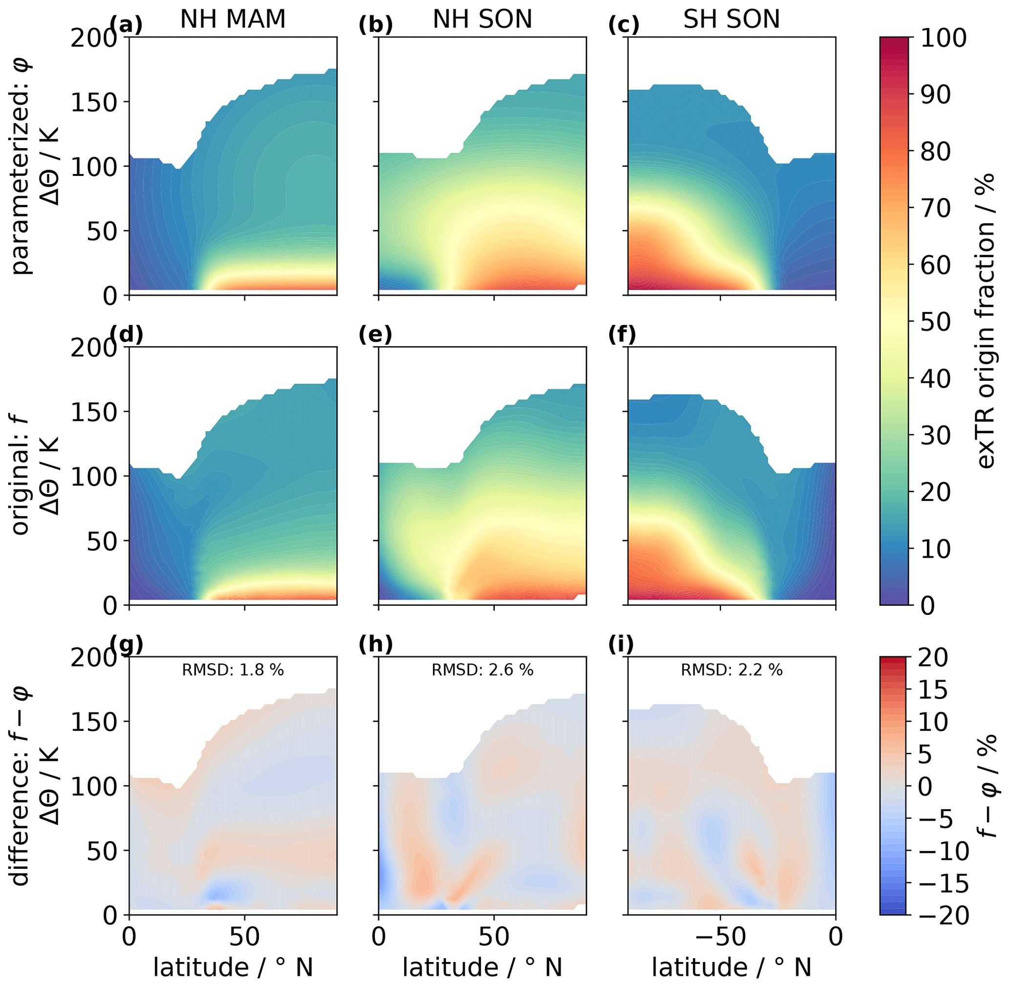
Figure 1Comparing seasonal–hemispheric extra-tropical origin fractions parameterization (φ, a–c) and original CLaMS origin fraction simulation results from Hauck et al. (2020) (f, d–f). The difference is shown in (g)–(h). Only three selected season–hemisphere combinations are shown here (NH MAM, a, d, g; NH SON, b, e, h; SH SON, c, f, i). The remaining distributions are shown in Fig. S1. Vertical coordinates are given in potential temperature above the 2 PVU tropopause (Δθ).
2.2.2 Entry region mixing ratio time series
Our new exTR–TR method uses a TR ground-reference time series together with constant time shift values txi in order to simulate reference time series in the three entry regions as defined by the origin fractions from Hauck et al. (2020) (see Eq. 4). This will work for inert monotonic tracers like SF6. In contrast, the entry region mixing ratio time series of tracers like CO2, which are characterized by a pronounced seasonality in the troposphere, most likely cannot be approximated satisfactorily with this approach. These tracers are thus not suited for deriving mean age with the exTR–TR method in the LMS. Here, we first describe which TR ground-reference time series we use and secondly, how we derived constant time shift values txi.
In this study, we use SF6 as an age tracer. Simmonds et al. (2020) used ground measurements from the AGAGE (Advanced Global Atmospheric Gases Experiment) network (Prinn et al., 2018) together with measurements of archived air samples and the 2-D AGAGE 12-box model (Cunnold et al., 1978, 1983; Rigby et al., 2013) to derive a monthly resolved time series of SF6 mixing ratios from the 1970s to 2018. We use the TR ground SF6 mixing ratios of an updated version of this dataset (Laube et al., 2022), which has been extended until the end of 2019, as a reference time series ) for calculating the mean age of air.
In order to derive txi for each of the three entry regions, we use the annual mean optimized 3-D SF6 mixing ratios output from the Model for Ozone and Related Tracers (MOZART v4.5) for 1970 to 2008, published by Rigby et al. (2010, Supplement). Rigby et al. (2010) derived a new estimate of SF6 emissions using the Emissions Database for Global Atmospheric Research (EDGAR v4) as a prior and optimizing the emissions using SF6 ground measurements from the AGAGE network including monitoring site data and archived sample measurements together with MOZART and meteorological data from the National Centers for Environmental Prediction/National Center for Atmospheric Research (NCEP/NCAR) reanalysis project. The annually averaged, 3-D optimized SF6 mixing ratio fields that we use to derive txi are part of their result. In our approach, we only considered the data from 1973 to 2008, since the data from 1970 to 1972 may be influenced by the start conditions of the model (Rigby et al., 2010). We calculated txi for each of the three entry regions following three steps:
- i.
Calculate a mean TR ground SF6 time series by using MOZART data between −30 to 30∘ N weighted by latitude.
- ii.
For each grid cell and each year of the 3-D SF6 field time series, interpolate SF6 mixing ratios to TR ground time using (i) and calculate time shift to TR ground.
- iii.
For each entry region, calculate mean and standard deviations weighted by latitude and pressure for time shifts from (ii) for 1973 to 2008 altogether to eventually obtain txi and information on associated uncertainty.
The latitudinal extents of the entry regions that we calculated txi for are the same as for the origin fractions by Hauck et al. (2020). For the exTR entry regions, we included data between 500 and 200 hPa. For the TR entry region, we included data between 300 and 100 hPa. Table 1 lists txi and standard deviations for the three entry regions SH exTR, TR and NH exTR. Positive values of txi indicate that the corresponding region lags behind TR ground SF6 mixing ratios. Note that for NH exTR, txi is negative. This means that this region precedes TR ground SF6 mixing ratios. This finding is consistent with SF6 source regions being located primarily in the Northern Hemisphere (Rigby et al., 2010).
We performed a Monte Carlo simulation in order to test whether txi can be considered constant over time for each entry region. Firstly, for each entry region, we calculated weighted means and standard deviations for each year (instead of for the whole time period as in iii). Figure 2 shows the resulting time shift time series from 1973 to 2008. Secondly, for each year, we took 10 000 samples from a Gaussian distribution using those weighted means and standard deviations in order to create 10 000 time series for each entry region. Thirdly, we applied a linear fit to each of the 10 000 time series and calculated the mean and the standard deviation of the slope for each entry region. The resulting mean slopes, standard deviations and the ratio of mean slope and standard deviation are listed in Table S1 in the Supplement. For NH exTR and TR, the mean slopes deviate less than 1 standard deviation from 0. For SH exTR, the mean slope deviates less than 1.2 standard deviations from 0. Hence, we do not detect a significant trend. These findings strengthen our confidence into our assumption that we can use the constant time shifts txi listed in Table 1 together with ) to describe the SF6 entry mixing ratio time series reasonably well. In the context of our exTR–TR method, we assume that this also holds true for the subsequent decade from 2008 on. This decade is not covered by the model from Rigby et al. (2010) that we used to derive txi, however, it is covered by ) (Laube et al., 2022, updated from Simmonds et al., 2020).
Previous studies used a similar procedure as outlined above (steps i–iii) to estimate transport timescales while referencing the NH midlatitude ground (Orbe et al., 2021; Waugh et al., 2013). We found that txi varies less over the time period 1973–2008 when referencing the tropical ground in the MOZART dataset. In order to derive more robust entry mixing ratio time series for our exTR–TR method, we thus decided to use the tropical ground as a reference. We emphasize that each txi as defined here is an integrated empirical measure. No useful information pertaining to transport paths or transit times from the TR ground to the entry regions is contained in txi. We only use txi to derive entry mixing ratio time series at locations where suitable long-term time series are not available from measurements.
Table 1txi and standard deviations for SF6 mixing ratio time series at three entry regions (NH 30–90∘ N, 500–200 hPa; TR 30∘ S–30∘ N, 300–100 hPa; SH 30–90∘ S, 500–200 hPa), weighted by latitude and pressure for the time period 1973–2008. These time shifts have been calculated relative to TR ground.
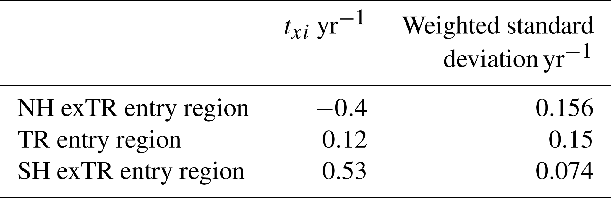
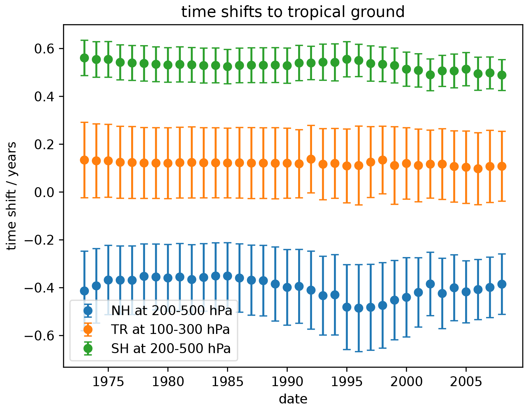
Figure 2Annual mean time shifts and standard deviations for SF6 mixing ratio time series at three entry regions, weighted by latitude and pressure. Based on 3-D annual SF6 model data output from Rigby et al. (2010).
2.3 Stratospheric observations of age tracer SF6
We apply our new exTR–TR method to in situ measurements of SF6 that were obtained during three HALO research campaigns. The first campaign, PGS (Oelhaf et al., 2019), is a combination of three missions: POLSTRACC (Polar Stratosphere in a Changing Climate), GW-LCYCLE (Investigation of the Life Cycle of Gravity Waves) and SALSA (Seasonality of Air mass transport and origin in the Lowermost Stratosphere). The PGS campaign was split into two campaign phases that were conducted in NH winter 2015–2016 between 13 December and 2 February and NH early spring 2016 between 26 February and 18 March. The second campaign, WISE (Wave-driven Isentropic Exchange, https://www.wise2017.de, last access: 5 May 2022), took place mainly in NH fall 2017 between September and October. The flight tracks of HALO during the PGS and WISE campaigns are shown in Figs. 2 and 1b of Keber et al. (2020). They cover large parts of midlatitudes and high latitudes in the NH. Thirdly, we consider data from the SouthTRAC (Southern Hemisphere Transport, Dynamics and Chemistry) campaign which took place in SH spring 2019. The SouthTRAC campaign was also split into two campaign phases, conducted between 6 September and 9 October (Rapp et al., 2021) and between 2 and 15 November. The flight tracks for SouthTRAC, which covered a wide geographical area of the SH, are shown in Jesswein et al. (2021).
Measurements of SF6 and CFC-12 were obtained in-flight in the context of all three campaigns with a time resolution of 1 min using the ECD channel of the two-channel Gas chromatograph for Observational Studies using Tracers (GhOST) instrument in a similar setup as used in the SPURT campaign (Bönisch et al., 2009; Engel et al., 2006). SF6 has been measured with a precision of 0.6 % (0.56 %) during SouthTRAC (PGS, WISE). CFC-12 has been measured with a precision of 0.23 % (0.2 %) during SouthTRAC (PGS, WISE). All measurements are reported relative to the AGAGE SIO-05 scale (Miller et al., 2008; Prinn et al., 2018; Rigby et al., 2010; Simmonds et al., 2020). Due to the better precision of CFC-12 measurements, the original SF6 data were smoothed using a local SF6–CFC-12 correlation 10 min before and after each measurement following Krause et al. (2018), prior to calculating mean age values. The height of the dynamical 2 PVU tropopause (e.g., Gettelman et al., 2011) as well as eq. lat. coordinates were obtained via CLaMS driven by ERA-5 reanalysis along the flight tracks. With this study, we exclusively focus on the LMS. Therefore, only tracer measurements at or above the dynamical tropopause were considered (i.e., with Δθ≥0 K). Tracer measurements and flight coordinates can be downloaded from Wagenhäuser et al. (2022). Additional data associated to the HALO aircraft campaigns that are beyond the scope of this study are accessible via the HALO database at https://halo-db.pa.op.dlr.de/ (last access: 30 March 2023; DLR, 2023).
We derive mean age in the LMS using in situ SF6 measurements from three aircraft campaigns (see Sect. 2.3). Results are presented in a 2-D tropopause-relative coordinate system. The potential temperature relative to the local dynamical tropopause (defined by the value of 2 PVU) Δθ is used as the vertical coordinate. Horizontally, data are sorted by eq. lat. In order to visualize and compare our results, datasets were processed in three steps:
-
Mean age was calculated for each data point that was measured above the local 2 PVU tropopause.
-
For each campaign dataset, mean ages were averaged in Δθ–eq. lat. bins (5 K – 5∘). Only bins that contained at least five data points were considered.
-
The averaged mean ages have been corrected for mesospheric loss using a linear correction function by Leedham Elvidge et al. (2018), given in their Fig. 4:
3.1 Method comparison using campaign-averaged results
We applied our new exTR–TR method for deriving mean age in the LMS considering exTR and TR input into the stratosphere to all three campaign datasets. Further, we applied the conventional TR-only method, which considers only TR input into the stratosphere, in order to compare the results from both methods. The results were averaged and corrected for mesospheric loss.
Figure 3 shows the resulting Δθ–eq. lat. distributions of averaged mean age mA for PGS (left column), WISE (middle column) and SouthTRAC (right column), derived using the conventional TR-only method mATR-only (top row), using our new exTR–TR method mAexTR−TR (middle row), and the difference between the two methods ΔmAmethods (bottom row). There are negative values down to −0.54 years close to the tropopause below Δθ=10 K in the WISE dataset using the TR-only method (panel b). In the same region, mean ages between −0.23 and 0.35 years are found using the new exTR–TR method (panel e). Mean ages below 0 as derived from the TR-only method do not allow for a reasonable interpretation regarding transport timescales in the LMS. In contrast, mean ages derived using our new exTR–TR method appear physically reasonable, even close to the tropopause. During the WISE campaign, low gradients in mAexTR−TR values reveal a well-mixed LMS (panel e), while during PGS and ST, stronger gradients in mAexTR−TR are found (panels d and f).
The maximum absolute difference between the average exTR–TR and TR-only methods' derived mean ages |ΔmAmethods| is 0.31 years (WISE and PGS) and 0.42 years (SouthTRAC) on the same order of magnitude for all three campaigns, but in different direction for the SH (see also Fig. 3, bottom row). For all three campaigns |ΔmAmethods| is largest close to the tropopause at midlatitudes and high latitudes and approaches 0 years further up and closer to the Equator. This distribution is similar to the distribution of exTR origin fractions from CLaMS. In fact, |ΔmAmethods| and the exTR origin fractions are highly correlated (r>0.99 for all three campaigns). This results from the design of the exTR–TR method, which explicitly considers exTR input into the stratosphere.
Note that in the SH data from the SouthTRAC campaign, mean ages are generally lower when derived using the exTR–TR method than when using the TR-only method. For NH data (WISE, PGS), the opposite is the case. This is a direct consequence from the TR ground mixing ratio time series being lagged by a positive (in the SH) and a negative (in the NH) empirical time shift to obtain the respective entry mixing ratio time series (see Table 1).
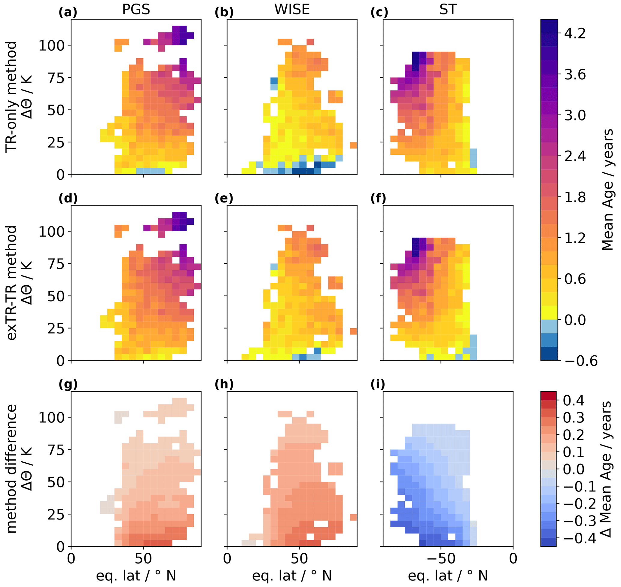
Figure 3Comparison of methods to derive mean age in the LMS during PGS (a, d, g), WISE (b, e, h) and SouthTRAC (c, f, i). Results are shown for the TR-only method (a–c) and the new exTR–TR method (d–f). The absolute differences between both methods are shown in (g)–(i). Altitude is given in Δθ. Horizontally, data are sorted by eq. lat.
3.2 SouthTRAC and PGS campaign: SH vs. NH late winter/early spring
The SouthTRAC and PGS campaigns both involved flights during the respective hemisphere's late winter or early spring. We compare results from the SouthTRAC campaign's phase 1 dataset (ST1) to results from the PGS campaign's phase 2 dataset (PGS2), derived with the exTR–TR method. This selection is a compromise between including a high number of trace gas measurements and having a large seasonal overlap between both datasets. Again, the results were averaged and corrected for mesospheric loss.
Figure 4 shows mAexTR−TR for ST1 (panel a), for PGS2 (panel b) and the difference between the two mAPGS2−ST1 (panel c). In order to calculate interhemispheric differences, the mAexTR−TR distribution from ST1 was converted from eq. lat. degrees North to eq. lat. degrees South by flipping it horizontally. Hence, the respective pole corresponds to 90∘ eq. lat. for both datasets in panel (c). Mean ages mAexTR−TR between −0.2 and 0.1 years are found within the lowest 10 K above the tropopause during ST1 (panel a). During PGS2, mAexTR−TR between 0.2 and 1.1 years are found in the equivalent region in the NH (panel b). The differences in mean age mAPGS2−ST1 (panel c) reveal higher mean ages during PGS2 than during ST1 from the tropopause up to 65 K above the tropopause throughout midlatitudes and high latitudes, with a few exceptions. On average, below Δθ=65 K, the LMS is 0.5±0.3 years older during PGS2 than during ST1. Above Δθ=65 K, a more complex picture is observed: at Δθ levels between 65 and 85 K at latitudes between 40 and 55∘, the LMS is even older during PGS2 than during ST1, with mA years on average. In contrast, the opposite is the case at the same Δθ levels but at poleward latitudes higher than 55∘: mean ages during ST1 are older than during PGS2, with mAPGS2−ST1 reaching values down to −2.1 years. A less clear picture emerges when comparing mean ages derived with the TR-only method (see Appendix C: Fig. C1). This could be explained by the fact that the TR-only method disregards the interhemispheric gradient in SF6 mixing ratios. In the LMS, the resulting mean age values are thus low biased in the NH, while they are old biased in the SH using the TR-only method. These biases happen to obscure interhemispheric differences in mean age in the LMS which have been detected using the new exTR–TR method on the same dataset.

Figure 4Comparison of mean age latitude–altitude distributions during SouthTRAC phase 1 (ST1) (a), PGS phase 2 (PGS2) (b). The hemispheric difference based on these two campaign phases is shown in panel (c). Altitude is given in Δθ. Horizontally, data are sorted by eq. lat.
Our findings indicate that on the one hand, during ST1, old air from higher altitudes descends in a confined way at high latitudes. There is a sharp vortex edge with a strong gradient in the SH. On the other hand, during PGS2, descending old air is mixed vertically and horizontally with young air in the LMS. The vortex edge is less sharp than during ST1, resulting in younger air at high latitudes and altitudes and older air outside the PGS2 vortex region compared to ST1.
These results cover only isolated time periods of less than 2 months for each campaign. In addition, as discussed by Jesswein et al. (2021), the extent of the respective polar vortices and therefore also the location of the respective vortex edge are likely to be different for both hemispheres. Hence, different vortex characteristics contribute to the differences observed in Fig. 4. Nevertheless, our findings are in agreement with multiannual simulation results from Konopka et al. (2015), who found a pronounced minimum in wave forcing driving the shallow branch of the BDC in the midlatitudes of the lower stratosphere in the SH between June and October, as opposed to a maximum in boreal spring in the NH.
3.3 Sensitivity study
3.3.1 Procedure
Our new exTR–TR method requires input of several parameters which all have individual uncertainties. In the following discussion, the sensitivity of the exTR–TR method to these uncertainties is investigated in the context of three aircraft campaigns.
We identified seven uncertain parameters:
- i.
extra-tropical origin fraction (fexTR,seas(x));
- ii.
time shift to extra-tropical entry region (texTR);
- iii.
time shift to tropical entry region (tTR);
- iv.
measurement precision of age tracer mixing ratios (χ(x));
- v.
ratio of moments (λ);
- vi.
chemical depletion of age tracer SF6;
- vii.
reference time series calibration-scale uncertainty.
Parameters (i) to (vi) may vary for each individual observational sample, making them eligible for a sensitivity analysis. In contrast, the uncertainty of the calibration scale of the reference time series (vii) affects all derived absolute mean ages, not in an individual but in a consistent way. Therefore, we excluded it from the sensitivity analysis, albeit knowing that it contributes to the overall uncertainty in deriving mean age from tracers. Furthermore, we excluded the chemical depletion of SF6 (vi) from the sensitivity analysis since it is not yet well understood and the subject of current comprehensive research (e.g., Loeffel et al., 2022). Leedham Elvidge et al. (2018) showed that younger mean age values derived from SF6 measurements, which point to shorter transport paths, are less affected by the mesospheric sink than older mean age values. Adequately addressing uncertainties in mean age due to the chemical depletion of SF6 is beyond the scope of this paper, which focuses primarily on young air in the LMS.
Parameters (i) to (v) are suited for a sensitivity analysis within the scope of this study using a Monte Carlo simulation. Since typical mean ages and origin fractions vary across different locations and seasons in the LMS, the sensitivity of the exTR–TR method is investigated and results are shown in the same 2-D tropopause-relative coordinate system that is used for the results shown in Sect. 3.1 and 3.2: Δθ is used as vertical coordinate, while horizontally, data are sorted by eq. lat. We conduct the sensitivity analysis by applying the following procedure to each of the three aircraft campaign datasets individually.
In order to obtain a reduced set of representative data and therefore reduce computational effort of the subsequent steps, SF6 mixing ratios and dates of observation are averaged into 5 K Δθ and 5∘ eq. lat. bins. For each bin, the following three steps are applied:
Step 1. For each uncertain parameter (i)–(v), a random number is drawn based on the parameter's best estimate and its uncertainty for that specific bin (see below for details). This is done 1000 times to create 1000 sets of parameters.
Step 2. These 1000 sets of parameters are used to calculate 1000 mean age values.
Step 3. The standard deviation of those 1000 mean age values is calculated to obtain an overall sensitivity value for this bin.
In this way, we derive the overall sensitivity. Further, we investigate the relative importance of the uncertain parameters (i)–(v). For this purpose, additional sensitivity calculations are done where only one uncertain parameter is varied while leaving the others at their best estimate.
3.3.2 Parameter uncertainties
Here, we describe how uncertainties associated with parameters (i)–(v) are implemented in step 1 of the sensitivity analysis.
- i.
The exTR origin fraction fexTR(x) varies spatially and over time. For each of the three aircraft campaigns, the spatial distribution of uncertainties in fexTR(x) is derived from the parameterized origin fraction φi,seas(x) (see Sect. 2.2.1) individually. Therefore, for each bin, the mean absolute half difference (MAHDseas) between φi,seas(x) and φi,next seas(x), respectively φi,previous seas(x), is calculated. In addition, the root mean squared difference (RMSDspace) between each bin and its eight surrounding bins is calculated. Both measures, MAHDseas and RMSDspace, are combined in the root sum squared to finally derive the spatial distribution of uncertainties in the exTR origin fraction for each campaign. Random values are drawn from a Gaussian distribution using this root sum squared.
- ii., iii.
Obtaining texTR for the NH and for the SH tropopause and tTR for the tropical tropopause regarding SF6 from the annually averaged 3-D model output is described in Sect. 2.2.2. We use the weighted mean values and standard deviations given in Table 1 as input for a Gaussian distribution from which random values are drawn.
- iv.
The measurement precision of age tracer mixing ratios χ(x) is given campaign-wise in Sect. 2.3. Since we use smoothed SF6 mixing ratios by considering local CFC-12–SF6 correlations for mean age calculations, we here apply the better measurement precision for CFC-12 mixing ratios to draw samples from a Gaussian distribution.
- v.
Regarding the ratio of moments λ, random values are drawn from a triangular distribution with a minimum of λ=0.7 years, a center of λ=1.2 years and a maximum of λ=2 years.
3.3.3 exTR–TR method sensitivities during PGS, WISE and SouthTRAC
The sensitivities of the exTR–TR method to uncertainties in input parameters have been calculated following the procedure outlined above. The resulting distributions of sensitivity values are shown in Fig. 5. The most sensitive regions are found between 20–40∘ poleward of the Equator below Δθ=20 K during all three aircraft campaigns with maximum values of 0.22 years (PGS, panel a), 0.19 years (WISE, panel b) and 0.16 years (SouthTRAC, panel c). Above Δθ=20 K, the sensitivity values are distributed evenly (standard deviation <0.02 years), with average values of 0.15 years (PGS) and 0.14 years (WISE and SouthTRAC). These sensitivities are lower than the differences between mean ages derived using the exTR–TR method and the TR-only method, which are found to be larger than 0.3 years close to the tropopause.
The contribution of the individual parameters (i)–(v) is shown in Fig. 6. Each row depicts isolated sensitivities to uncertainties in a single parameter with all other parameters being held at their best estimate. This allows us to test the relative importance of the individual parameters to the exTR–TR method's overall sensitivity. Most strikingly, uncertainties in the ratio of moments (parameter v) seem to contribute only negligibly to the overall sensitivity (panels m–o). Measurement uncertainties in the stratospheric mixing ratio χ(x) contribute to the overall sensitivity spatially evenly distributed to a moderate extent (panels j–l). Due to the slightly worse measurement precision during SouthTRAC and in addition due to the decelerating relative growth rate of SF6 mixing ratios, the uncertainties in χ(x) have a stronger impact on the overall sensitivity during SouthTRAC than during the other two campaigns. In the upper part of the LMS (above Δθ=50 K), uncertainties in tTR dominate the overall sensitivity (panels g–i). Below, uncertainties in texTR and in fexTR(x) gain importance (panels a–f). Note that the SH uncertainties in texTR are low (see Table 1), which is reflected by contributing to the overall sensitivity during the SouthTRAC campaign (panel f) only to a minor to moderate extent.
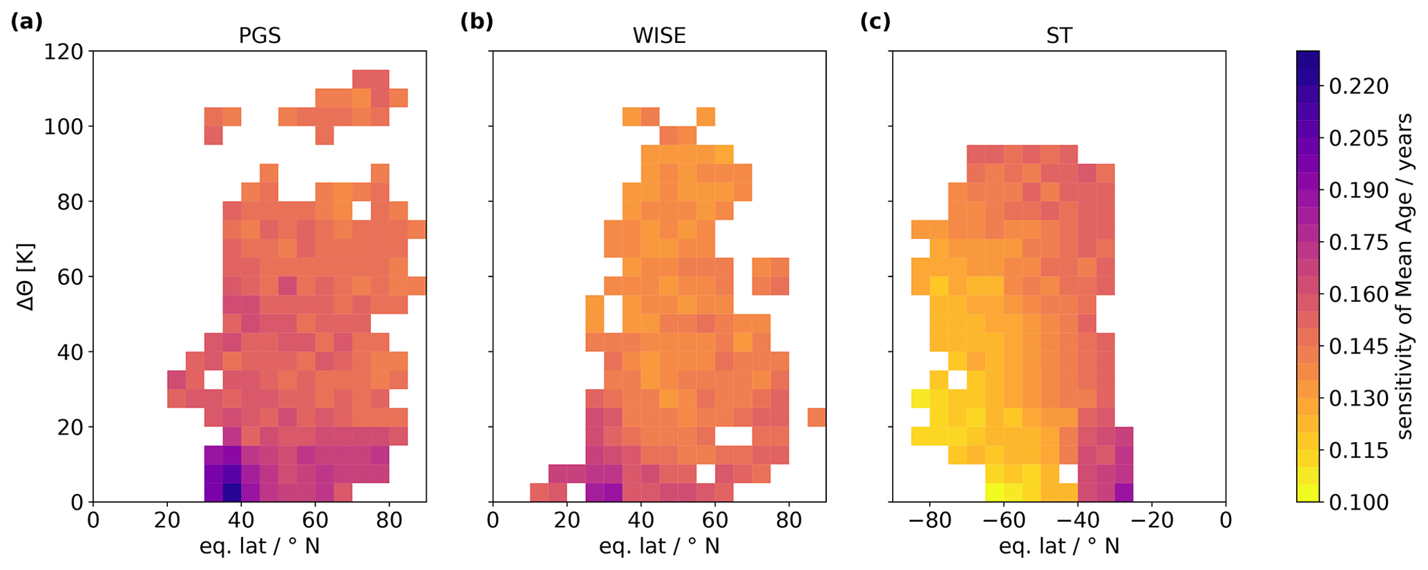
Figure 5Latitude–altitude distribution of sensitivities of mean age from the exTR–TR method to uncertainties in all considered input parameters, calculated for PGS (a), WISE (b) and SouthTRAC (c) campaigns. Altitude is given in Δθ. Horizontally, data are sorted by eq. lat.
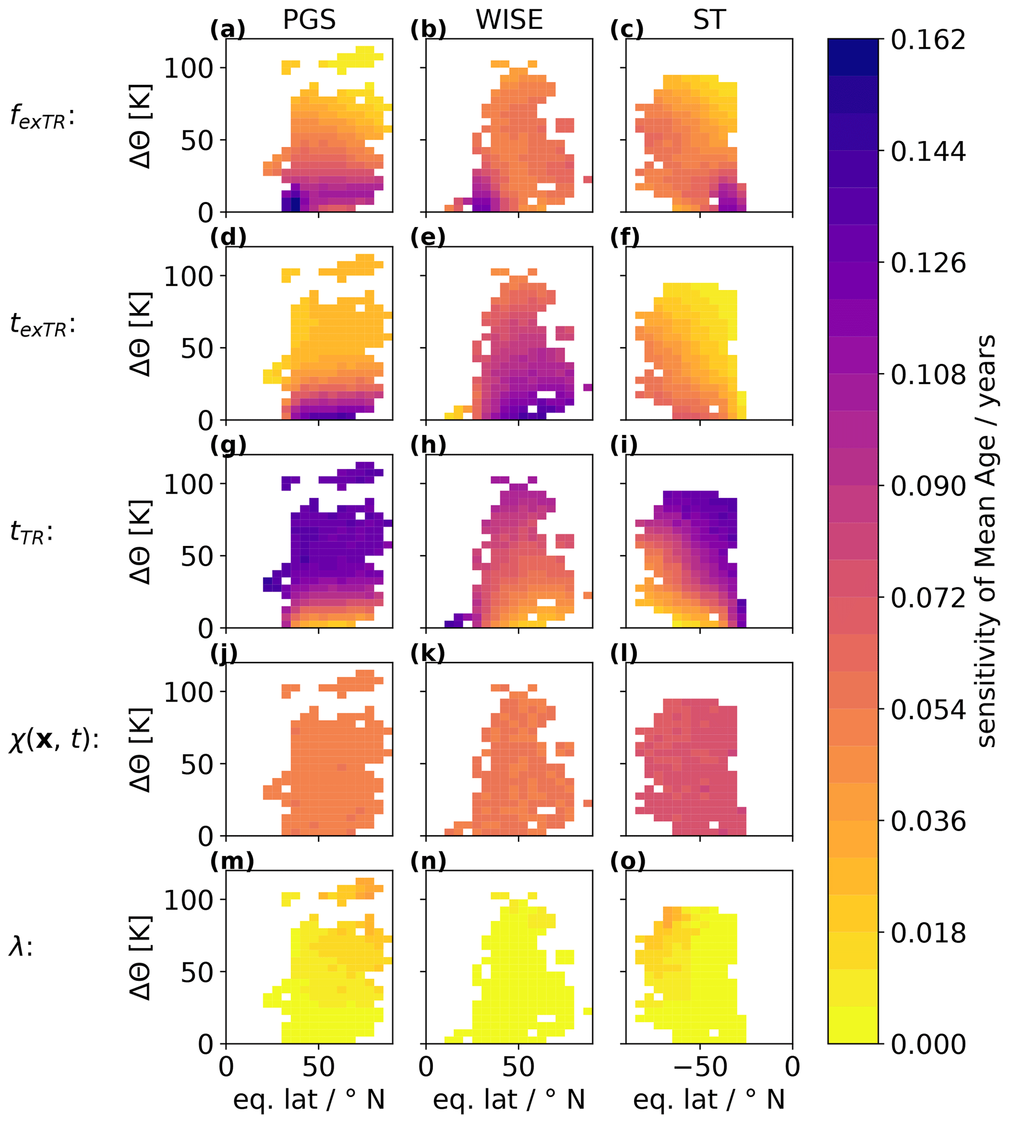
Figure 6As Fig. 5, but each uncertain parameter is considered independently, assuming the others to be accurate. Uncertain parameters: exTR origin fraction (fexTR, a–c), time shift to exTR entry region (texTR, d–f), time shift to TR entry region (tTR, g–i), SF6 mixing ratio measurement uncertainty (χ(x), j–l) and the ratio of moments (λ, m–o).
In this work, the new exTR–TR method to derive stratospheric mean age of air in the LMS from observational tracer mixing ratio data is presented. In order to take exTR input into the stratosphere into account, our implementation of the exTR–TR method uses seasonally averaged exTR origin fractions from CLaMS (Hauck et al., 2020), for which we provide a parameterization, and a long-term tracer mixing ratio time series for each entry region . Following Hauck et al. (2020), the entry regions are defined as a northern (90–30∘ N), a TR (30∘ N–30∘ S) and a southern (30–90∘ S) tropopause section. Owing to the lack of continuous long-term measurements of age tracers at the tropopause, we approximated by applying a constant empirical time shift txi to the available TR ground tracer mixing ratio time series for each entry region. For the age tracer SF6, individual txi were obtained in this study by averaging optimized 3-D model output between 1973–2008 that was published by Rigby et al. (2010). We emphasize that the resulting txi are exclusively used to approximate and that they do not represent real-world transport times between TR ground and the entry regions.
We applied the exTR–TR method to in situ SF6 measurements taken during three aircraft campaigns in different geographical regions and at different times: PGS in NH late winter or early spring 2016, WISE in NH fall 2017 and SouthTRAC in SH early spring 2019. The resulting mean age values were averaged into bins over multiple flights using tropopause-relative altitude and eq. lat. coordinates (Δθ bins of size 5 K, eq. lat. bins of size 5∘). These averaged mean age values were corrected for mesospheric loss by applying a linear function published by Leedham Elvidge et al. (2018). In addition, the conventional TR-only method, which assumes that all air enters the stratosphere through the TR tropopause, was applied to the same data and the results were post-processed in the same way in order to compare the results. Using the conventional TR-only method, negative mean age values are derived in the LMS close to the tropopause during the WISE campaign. Using the new exTR–TR method instead, the number and extent of negative mean age values are reduced. Maximum absolute differences between the resulting averaged mean age values from the two methods range from 0.31 to 0.42 years among the three campaigns and go in different directions for the two hemispheres. With our new exTR–TR method, we are thus able to derive more realistic values of typical transport times in the LMS from measurements. This allows a comparison of the two hemispheres based on campaign data. We compared results derived using the exTR–TR method from the PGS campaign phase 2 (PGS2) to SouthTRAC campaign phase 1 (ST1) in order to investigate hemispheric differences with a maximal seasonal overlap of the campaigns. On average, below Δθ=65 K, the LMS was 0.5±0.3 years older during PGS2 than during ST1 across all eq. lats that are covered by both datasets. We attribute this older LMS to mixing with old vortex air during PGS2, as opposed to a more confined vortex edge with higher age gradients during ST1. Although these findings only cover an isolated time period of less than 2 months for each campaign and do not account for different polar vortex characteristics, they are in agreement with multiannual simulation results from Konopka et al. (2015), who found a pronounced minimum in wave forcing driving the shallow branch of the BDC in the midlatitudes of the lower stratosphere in the SH between June and October, as opposed to a maximum in boreal spring in the NH.
The sensitivity of the exTR–TR method to uncertainties of six input parameters was investigated at different locations using a Monte Carlo approach. The mesospheric loss of SF6 was excluded from this sensitivity analysis since it is currently not well understood and beyond the scope of this work. The combined sensitivity was found to be less than 0.22 years for all locations for all three campaigns. The most sensitive region for each hemisphere was located between 20–40∘ poleward of the Equator below Δθ=20 K. This is related to the setup of the experiment with a boundary at 30∘ in each hemisphere. Uncertainties in the origin fractions and in txi have the largest isolated impact on the sensitivity of the exTR–TR method. Overall, these sensitivities are lower than the differences between mean ages derived using the exTR–TR method and the TR-only method. Hence, our new exTR–TR method yields mean age values that differ considerably from results obtained using the conventional TR-only method in the LMS. In future studies, the exTR–TR method could be used to improve deriving estimates of total and inorganic chlorine from observations of organic chlorine in the LMS as in Jesswein et al. (2021).
In the case of an ideal inert linear evolving tracer, the tropical ground time series as a function of transit time t is given by
The negative sign indicates that looking at increasing transit times means looking backwards in time.
Assuming a constant time shift txi for each entry region i, the tracer time series at xi is
Considering individual transit time distributions for each origin fraction fi(x), the stratospheric mixing ratio χ(x) of a suitable age tracer at an arbitrary location x in the stratosphere is
Hence, by inserting Eq. (A2) into Eq. (A3), the stratospheric mixing ratio can be expressed as
The mean age Γ is the first moment of the age spectrum, given by
In the case of , Eq. (A5) translates into the mean age of air originating from source region i (Γi(x)):
Inserting Eq. (A6) into Eq. (A4) yields the following:
Since the sum of all origin fractions equals 1, Eq. (A7) can also be written as
The mean age Γ(x) equals the sum of individual Γi(x), weighted by their respective origin fraction fi(x):
By inserting Eq. (A9) into Eq. (A8), we can thus reduce the number of unknown parameters:
Equation (A10) can be solved for Γ, which yields
which is equivalent to Eq. (5). The same result can be obtained mathematically when we use the origin fractions as weights only for the mixing ratio time series and neglect the concept of (starting with Eq. 2 instead of Eq. A3). Differences across individual thus have no influence on calculating the mean age from an ideal inert linear evolving tracer. In contrast, in the case of an ideal inert quadratic evolving tracer, the Ansatz expressed in Eq. (A3) cannot be solved for Γ(x) without knowledge of individual Γi(x). However, if the quadratic term of the tracer mixing ratio time series is sufficiently low, then the concept of can be neglected by using the Ansatz expressed in Eq. (2).
In order to derive mean age from an ideal inert quadratic evolving tracer with multiple entry regions, we extended the equations given by Volk et al. (1997). In this case, the TR ground mixing ratio time series is given as a function of transit time by
Assuming a constant time shift txi for each entry region i, the tracer time series at xi is
Hence, by inserting Eq. (A13) into Eq. (2), the stratospheric mixing ratio can be expressed as
which is equivalent to
Note that for better readability, fi(x) is written as fi.
By extracting constant factors from the integral and applying Eq. (A5), Eq. (A15) can also be written as
The width of the age spectrum Δ is the square root of the second centered moment of the age spectrum, which is given by
Equation (A17) can be transformed to
Inserting Eq. (A18) into Eq. (A16) yields
Since the sum of all origin fractions equals 1 and with the weighted mean time shift , Eq. (A19) can also be written as:
Inserting the ratio of moments into Eq. (A20) yields the quadratic equation Eq. (A21):
which can be rearranged to
and finally solved for Γ:
We designed a general mathematical parameterization function φi,seas with 12 parameters to derive 2-D parameterizations for exTR origin fractions in ΔΘ−eq. lat. space. The process of designing φi,seas was guided by a non-physical but entirely geometrical approach pursuing three priorities for each of the 10 considered fi,seas(x) at once:
- i.
φi,seas should be able to reproduce major geometrical features of the distributions.
- ii.
The maximum difference between φi,seas(x) and fi,seas(x) should be as low as possible.
- iii.
The mean deviation between φi,seas(x) and fi,seas(x) should be as low as possible.
In addition to the three priorities, the number of parameters needed to achieve (i), (ii) and (iii) should preferably be low. The resulting general mathematical parameterization function is a combination of Gaussian distributions and cumulative Gumbel distributions with 12 parameters in total:
The seasonally averaged fi,seas(x) data published by Hauck et al. (2020) are gridded in 2∘ latitude and 37 vertical potential temperature levels between 280 and 3000 K. Additionally, the difference in potential temperature to the local tropopause (ΔΘ) is provided for each data point. In order to find optimal fitting parameters using a least-square fit, for each of the 10 considered fi,seas(x) we only considered data from the respective hemisphere and for the lower 20 vertical levels (i.e., 280 to 480 K). The resulting parameters for each of the 10 considered fi,seas(x) are listed in Table B1. The Python code for applying φi,seas as given in Eq. (B4) and automatically including the information given in Table B1 is available from Wagenhäuser (2022a).
Table B1Parameter values for extra-tropical origin fractions φi,seas calculated with Eq. (B4) by hemisphere and season.
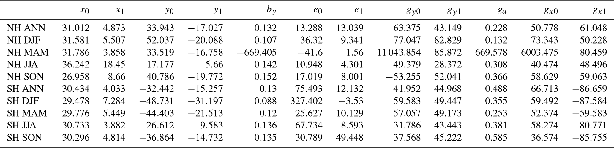
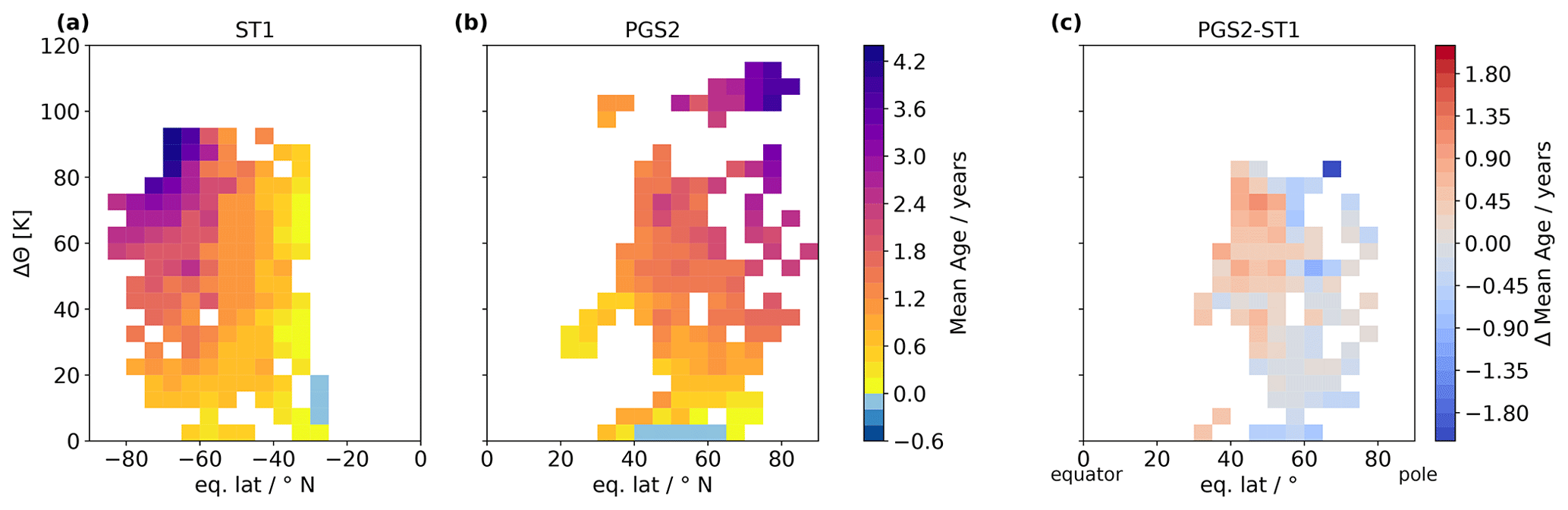
Figure C1Same as Fig. 4, but mean ages have been derived using the conventional TR-only method instead.
The Python software implementation of the exTR–TR method is available at https://doi.org/10.5281/zenodo.7267203 (Wagenhäuser and Engel, 2022).
The Python software code repository “f_exTR” for deploying our parameterizations of the CLaMS origin fractions is available at https://doi.org/10.5281/zenodo.7267114 (Wagenhäuser, 2022a).
The Python software code repository “sf6-timeshifts-from-rigby2010” for deriving SF6 time shifts to tropical ground using model data from Rigby et al. (2010) (Sect. 2.2.2) is available at https://doi.org/10.5281/zenodo.7267089 (Wagenhäuser, 2022b).
Tracer measurements, flight coordinates and mean age values derived using both the exTR–TR method and the TR-only method can be downloaded at https://doi.org/10.5281/zenodo.7275822 (Wagenhäuser et al., 2022).
The supplement related to this article is available online at: https://doi.org/10.5194/acp-23-3887-2023-supplement.
TW developed the mathematical framework and Python software code for the exTR–TR method in close collaboration with AE. AE initiated this study. TW, MJ, TK, TS, and AE operated the GhOST instrument during the SouthTRAC campaign. TW wrote the paper in collaboration with AE. All authors contributed to the final version of the paper.
The contact author has declared that none of the authors has any competing interests.
Publisher's note: Copernicus Publications remains neutral with regard to jurisdictional claims in published maps and institutional affiliations.
We would like to thank the DLR staff for the operation of the HALO and the support during all three campaigns. Many thanks also to all former master students at the Goethe University of Frankfurt, who helped to carry out measurements during the campaigns. Moreover, we thank Jens-Uwe Grooß for facilitating access to model-based Δθ and eq. lat. data along the flight tracks. We thank Matthew Rigby and Luke Western for providing updated AGAGE 12-box model output of SF6 mixing ratios. We further thank Ronald Prinn, Ray Weiss, Paul Krummel, Dickon Young, Simon O'Doherty, and Jens Mühle for facilitating access to the AGAGE data (http://agage.mit.edu, last access: 30 March 2023). The AGAGE stations used in this paper are supported by the National Aeronautics and Space Administration (NASA). Support also comes from the UK Department for Business, Energy & Industrial Strategy (BEIS) for MHD, the National Oceanic and Atmospheric Administration (NOAA) for RPB, and the Commonwealth Scientific and Industrial Research Organization (CSIRO) and the Bureau of Meteorology (Australia) for CGO.
This research was supported under the Deutsche Forschungsgemeinschaft (DFG,
German Research Foundation) Priority Program SPP 1294 “Atmospheric and Earth
System Research with HALO” – “High Altitude and Long Range Research
Aircraft” (project nos. EN367/5, EN367/8, EN367/11, EN367/13, EN367/14, and EN367/16). Financial support also came from the DFG – TRR 301 (project ID 428312742) and the National Aeronautics and Space Administration (NASA)
(grant nos. NNX16AC98G to MIT, and NNX16AC97G and NNX16AC96G to SIO).
This open-access publication was funded by the Goethe University Frankfurt.
This paper was edited by Rolf Müller and reviewed by three anonymous referees.
Andrews, A. E., Boering, K. A., Daube, B. C., Wofsy, S. C., Hintsa, E. J., Weinstock, E. M., and Bui, T. P.: Empirical age spectra for the lower tropical stratosphere from in situ observations of CO2: Implications for stratospheric transport, J. Geophys. Res.-Atmos., 104, 26581–26595, https://doi.org/10.1029/1999JD900150, 1999.
Andrews, A. E., Boering, K. A., Wofsy, S. C., Daube, B. C., Jones, D. B., Alex, S., Loewenstein, M., Podolske, J. R. and Strahan, S. E.: Empirical age spectra for the midlatitude lower stratosphere from in situ observations of CO2: Quantitative evidence for a subtropical “barrier” to horizontal transport, J. Geophys. Res.-Atmos., 106, 10257–10274, https://doi.org/10.1029/2000JD900703, 2001.
Birner, T. and Bönisch, H.: Residual circulation trajectories and transit times into the extratropical lowermost stratosphere, Atmos. Chem. Phys., 11, 817–827, https://doi.org/10.5194/acp-11-817-2011, 2011.
Bönisch, H., Engel, A., Curtius, J., Birner, Th., and Hoor, P.: Quantifying transport into the lowermost stratosphere using simultaneous in-situ measurements of SF6 and CO2, Atmos. Chem. Phys., 9, 5905–5919, https://doi.org/10.5194/acp-9-5905-2009, 2009.
Butchart, N.: The Brewer-Dobson circulation, Rev. Geophys., 52, 157–184, https://doi.org/10.1002/2013RG000448, 2014.
Cunnold, D., Alyea, F., and Prinn, R.: A methodology for determining the atmospheric lifetime of fluorocarbons, J. Geophys. Res., 83, 5493, https://doi.org/10.1029/JC083iC11p05493, 1978.
Cunnold, D. M., Prinn, R. G., Rasmussen, R. A., Simmonds, P. G., Alyea, F. N., Cardelino, C. A., and Crawford, A. J.: The Atmospheric Lifetime Experiment: 4. Results for CF2 Cl2 based on three years data, J. Geophys. Res., 88, 8401, https://doi.org/10.1029/JC088iC13p08401, 1983.
DLR, German Aerospace Center: The High Altitude and LOng Range database (HALO-DB), https://halo-db.pa.op.dlr.de/, last access: 16 February 2023.
Engel, A., Bönisch, H., Brunner, D., Fischer, H., Franke, H., Günther, G., Gurk, C., Hegglin, M., Hoor, P., Königstedt, R., Krebsbach, M., Maser, R., Parchatka, U., Peter, T., Schell, D., Schiller, C., Schmidt, U., Spelten, N., Szabo, T., Weers, U., Wernli, H., Wetter, T., and Wirth, V.: Highly resolved observations of trace gases in the lowermost stratosphere and upper troposphere from the Spurt project: an overview, Atmos. Chem. Phys., 6, 283–301, https://doi.org/10.5194/acp-6-283-2006, 2006.
Engel, A., Bönisch, H., Ullrich, M., Sitals, R., Membrive, O., Danis, F., and Crevoisier, C.: Mean age of stratospheric air derived from AirCore observations, Atmos. Chem. Phys., 17, 6825–6838, https://doi.org/10.5194/acp-17-6825-2017, 2017.
Fritsch, F., Garny, H., Engel, A., Bönisch, H., and Eichinger, R.: Sensitivity of age of air trends to the derivation method for non-linear increasing inert SF6, Atmos. Chem. Phys., 20, 8709–8725, https://doi.org/10.5194/acp-20-8709-2020, 2020.
Gettelman, A., Hoor, P., Pan, L. L., Randel, W. J., Hegglin, M. I., and Birner, T.: The extratropical upper troposphere and lower stratosphere, Rev. Geophys., 49, RG3003, https://doi.org/10.1029/2011RG000355, 2011.
Hall, T. M. and Plumb, R. A.: Age as a diagnostic of stratospheric transport, J. Geophys. Res., 99, 1059–1070, https://doi.org/10.1029/93JD03192, 1994.
Hauck, M., Fritsch, F., Garny, H., and Engel, A.: Deriving stratospheric age of air spectra using an idealized set of chemically active trace gases, Atmos. Chem. Phys., 19, 5269–5291, https://doi.org/10.5194/acp-19-5269-2019, 2019.
Hauck, M., Bönisch, H., Hoor, P., Keber, T., Ploeger, F., Schuck, T. J., and Engel, A.: A convolution of observational and model data to estimate age of air spectra in the northern hemispheric lower stratosphere, Atmos. Chem. Phys., 20, 8763–8785, https://doi.org/10.5194/acp-20-8763-2020, 2020.
Jesswein, M., Bozem, H., Lachnitt, H.-C., Hoor, P., Wagenhäuser, T., Keber, T., Schuck, T., and Engel, A.: Comparison of inorganic chlorine in the Antarctic and Arctic lowermost stratosphere by separate late winter aircraft measurements, Atmos. Chem. Phys., 21, 17225–17241, https://doi.org/10.5194/acp-21-17225-2021, 2021.
Keber, T., Bönisch, H., Hartick, C., Hauck, M., Lefrancois, F., Obersteiner, F., Ringsdorf, A., Schohl, N., Schuck, T., Hossaini, R., Graf, P., Jöckel, P., and Engel, A.: Bromine from short-lived source gases in the extratropical northern hemispheric upper troposphere and lower stratosphere (UTLS), Atmos. Chem. Phys., 20, 4105–4132, https://doi.org/10.5194/acp-20-4105-2020, 2020.
Kida, H.: General Circulation of Air Parcels and Transport Characteristics Derived from a hemispheric GCM, J. Meteorol. Soc. Japan. Ser. II, 61, 171–187, https://doi.org/10.2151/jmsj1965.61.2_171, 1983.
Konopka, P., Ploeger, F., Tao, M., Birner, T., and Riese, M.: Hemispheric asymmetries and seasonality ofmean age of air in the lower stratosphere: Deep versus shallow branch of the Brewer-Dobson circulation, J. Geophys. Res., 120, 2053–2066, https://doi.org/10.1002/2014JD022429, 2015.
Krause, J., Hoor, P., Engel, A., Plöger, F., Grooß, J.-U., Bönisch, H., Keber, T., Sinnhuber, B.-M., Woiwode, W., and Oelhaf, H.: Mixing and ageing in the polar lower stratosphere in winter 2015–2016, Atmos. Chem. Phys., 18, 6057–6073, https://doi.org/10.5194/acp-18-6057-2018, 2018.
Laube, J. C., Tegtmeier, S., Fernandez, R. P., Harrison, J., Hu, L., Krummel, P., Mahieu, E., Park, S., and Western, L.: Update on Ozone-Depleting Substances (ODSs) and Other Gases of Interest to the Montreal Protocol, chap. 1, in: Scientific Assessment of Ozone Depletion: 2022, GAW Report No. 278, edited by: Engel, A. and Yao, B., 509 pp., World Meteorological Organization, Geneva, Switzerland, 51–113, ISBN 978-9914-733-97-6, 2022.
Leedham Elvidge, E. C., Bönisch, H., Brenninkmeijer, C. A. M., Engel, A., Fraser, P. J., Gallacher, E., Langenfelds, R., Mühle, J., Oram, D. E., Ray, E. A., Ridley, A. R., Röckmann, T., Sturges, W. T., Weiss, R. F., and Laube, J. C.: Evaluation of stratospheric age of air from CF4, C2F6, C3F8, CHF3, HFC-125, HFC-227ea and SF6; implications for the calculations of halocarbon lifetimes, fractional release factors and ozone depletion potentials, Atmos. Chem. Phys., 18, 3369–3385, https://doi.org/10.5194/acp-18-3369-2018, 2018.
Loeffel, S., Eichinger, R., Garny, H., Reddmann, T., Fritsch, F., Versick, S., Stiller, G., and Haenel, F.: The impact of sulfur hexafluoride (SF6) sinks on age of air climatologies and trends, Atmos. Chem. Phys., 22, 1175–1193, https://doi.org/10.5194/acp-22-1175-2022, 2022.
Miller, B. R., Weiss, R. F., Salameh, P. K., Tanhua, T., Greally, B. R., Mühle, J., and Simmonds, P. G.: Medusa: A Sample Preconcentration and GC/MS Detector System for in Situ Measurements of Atmospheric Trace Halocarbons, Hydrocarbons, and Sulfur Compounds, Anal. Chem., 80, 1536–1545, https://doi.org/10.1021/ac702084k, 2008.
Oelhaf, H., Sinnhuber, B., Woiwode, W., Bönisch, H., Bozem, H., Engel, A., Fix, A., Friedl-Vallon, F., Grooß, J., Hoor, P., Johansson, S., Jurkat-Witschas, T., Kaufmann, S., Krämer, M., Krause, J., Kretschmer, E., Lörks, D., Marsing, A., Orphal, J., Pfeilsticker, K., Pitts, M., Poole, L., Preusse, P., Rapp, M., Riese, M., Rolf, C., Ungermann, J., Voigt, C., Volk, C. M., Wirth, M., Zahn, A., and Ziereis, H.: POLSTRACC: Airborne Experiment for Studying the Polar Stratosphere in a Changing Climate with the High Altitude and Long Range Research Aircraft (HALO), B. Am. Meteorol. Soc., 100, 2634–2664, https://doi.org/10.1175/BAMS-D-18-0181.1, 2019.
Orbe, C., Holzer, M., Polvani, L. M., and Waugh, D.: Air-mass origin as a diagnostic of tropospheric transport, J. Geophys. Res.-Atmos., 118, 1459–1470, https://doi.org/10.1002/jgrd.50133, 2013.
Orbe, C., Waugh, D. W., and Newman, P. A.: Air-mass origin in the tropical lower stratosphere: The influence of Asian boundary layer air, Geophys. Res. Lett., 42, 4240–4248, https://doi.org/10.1002/2015GL063937, 2015.
Orbe, C., Waugh, D. W., Montzka, S., Dlugokencky, E. J., Strahan, S., Steenrod, S. D., Strode, S., Elkins, J. W., Hall, B., Sweeney, C., Hintsa, E. J., Moore, F. L., and Penafiel, E.: Tropospheric Age-of-Air: Influence of SF6 Emissions on Recent Surface Trends and Model Biases, J. Geophys. Res.-Atmos., 126, 1–16, https://doi.org/10.1029/2021JD035451, 2021.
Plumb, R. A.: Stratospheric transport, J. Meteorol. Soc. Japan, 80, 793–809, https://doi.org/10.2151/jmsj.80.793, 2002.
Pommrich, R., Müller, R., Grooß, J.-U., Konopka, P., Ploeger, F., Vogel, B., Tao, M., Hoppe, C. M., Günther, G., Spelten, N., Hoffmann, L., Pumphrey, H.-C., Viciani, S., D'Amato, F., Volk, C. M., Hoor, P., Schlager, H., and Riese, M.: Tropical troposphere to stratosphere transport of carbon monoxide and long-lived trace species in the Chemical Lagrangian Model of the Stratosphere (CLaMS), Geosci. Model Dev., 7, 2895–2916, https://doi.org/10.5194/gmd-7-2895-2014, 2014.
Prinn, R. G., Weiss, R. F., Arduini, J., Arnold, T., DeWitt, H. L., Fraser, P. J., Ganesan, A. L., Gasore, J., Harth, C. M., Hermansen, O., Kim, J., Krummel, P. B., Li, S., Loh, Z. M., Lunder, C. R., Maione, M., Manning, A. J., Miller, B. R., Mitrevski, B., Mühle, J., O'Doherty, S., Park, S., Reimann, S., Rigby, M., Saito, T., Salameh, P. K., Schmidt, R., Simmonds, P. G., Steele, L. P., Vollmer, M. K., Wang, R. H., Yao, B., Yokouchi, Y., Young, D., and Zhou, L.: History of chemically and radiatively important atmospheric gases from the Advanced Global Atmospheric Gases Experiment (AGAGE), Earth Syst. Sci. Data, 10, 985–1018, https://doi.org/10.5194/essd-10-985-2018, 2018.
Rapp, M., Kaifler, B., Dörnbrack, A., Gisinger, S., Mixa, T., Reichert, R., Kaifler, N., Knobloch, S., Eckert, R., Wildmann, N., Giez, A., Krasauskas, L., Preusse, P., Geldenhuys, M., Riese, M., Woiwode, W., Friedl-Vallon, F., Sinnhuber, B.-M., de la Torre, A., Alexander, P., Hormaechea, J. L., Janches, D., Garhammer, M., Chau, J. L., Conte, J. F., Hoor, P., and Engel, A.: SOUTHTRAC-GW: An Airborne Field Campaign to Explore Gravity Wave Dynamics at the World's Strongest Hotspot, B. Am. Meteorol. Soc., 102, E871–E893, https://doi.org/10.1175/BAMS-D-20-0034.1, 2021.
Ray, E. A., Moore, F. L., Elkins, J. W., Rosenlof, K. H., Laube, J. C., Röckmann, T., Marsh, D. R., and Andrews, A. E.: Quantification of the SF6 lifetime based on mesospheric loss measured in the stratospheric polar vortex, J. Geophys. Res., 122, 4626–4638, https://doi.org/10.1002/2016JD026198, 2017.
Ray, E. A., Atlas, E. L., Schauffler, S., Chelpon, S., Pan, L., Bönisch, H., and Rosenlof, K. H.: Age spectra and other transport diagnostics in the North American monsoon UTLS from SEAC4RS in situ trace gas measurements, Atmos. Chem. Phys., 22, 6539–6558, https://doi.org/10.5194/acp-22-6539-2022, 2022.
Rigby, M., Mühle, J., Miller, B. R., Prinn, R. G., Krummel, P. B., Steele, L. P., Fraser, P. J., Salameh, P. K., Harth, C. M., Weiss, R. F., Greally, B. R., O'Doherty, S., Simmonds, P. G., Vollmer, M. K., Reimann, S., Kim, J., Kim, K.-R., Wang, H. J., Olivier, J. G. J., Dlugokencky, E. J., Dutton, G. S., Hall, B. D., and Elkins, J. W.: History of atmospheric SF6 from 1973 to 2008, Atmos. Chem. Phys., 10, 10305–10320, https://doi.org/10.5194/acp-10-10305-2010, 2010.
Rigby, M., Prinn, R. G., O'Doherty, S., Montzka, S. A., McCulloch, A., Harth, C. M., Mühle, J., Salameh, P. K., Weiss, R. F., Young, D., Simmonds, P. G., Hall, B. D., Dutton, G. S., Nance, D., Mondeel, D. J., Elkins, J. W., Krummel, P. B., Steele, L. P., and Fraser, P. J.: Re-evaluation of the lifetimes of the major CFCs and CH3CCl3 using atmospheric trends, Atmos. Chem. Phys., 13, 2691–2702, https://doi.org/10.5194/acp-13-2691-2013, 2013.
Simmonds, P. G., Rigby, M., Manning, A. J., Park, S., Stanley, K. M., McCulloch, A., Henne, S., Graziosi, F., Maione, M., Arduini, J., Reimann, S., Vollmer, M. K., Mühle, J., O'Doherty, S., Young, D., Krummel, P. B., Fraser, P. J., Weiss, R. F., Salameh, P. K., Harth, C. M., Park, M.-K., Park, H., Arnold, T., Rennick, C., Steele, L. P., Mitrevski, B., Wang, R. H. J., and Prinn, R. G.: The increasing atmospheric burden of the greenhouse gas sulfur hexafluoride (SF6), Atmos. Chem. Phys., 20, 7271–7290, https://doi.org/10.5194/acp-20-7271-2020, 2020.
Volk, C. M., Elkins, J. W., Fahey, D. W., Dutton, G. S., Gilligan, J. M., Loewenstein, M., Podolske, J. R., Chan, K. R., and Gunson, M. R.: Evaluation of source gas lifetimes from stratospheric observations, J. Geophys. Res.-Atmos., 102, 25543–25564, https://doi.org/10.1029/97jd02215, 1997.
Wagenhäuser, T.: AtmosphericAngels/f_exTR: v.1.0.0, Zenodo [code], https://doi.org/10.5281/zenodo.7267114, 2022a.
Wagenhäuser, T.: AtmosphericAngels/sf6-timeshifts-from-rigby2010: v1.0.0, Zenodo [code], https://doi.org/10.5281/zenodo.7267089, 2022b.
Wagenhäuser, T. and Engel, A.: AtmosphericAngels/exTR-TR-method: v.1.0.0, Zenodo [code], https://doi.org/10.5281/zenodo.7267203, 2022.
Wagenhäuser, T., Jesswein, M., Keber, T., Schuck, T., Engel, A., and Grooß, J.-U.: SF6 and CFC-12 measurements and mean age along HALO flight tracks during PGS, WISE and SouthTRAC, Zenodo [data set], https://doi.org/10.5281/zenodo.7275822, 2022.
Waugh, D. W. and Hall, T. M.: Age of stratospheric air: Theory, observations, and models, Rev. Geophys., 40, 1-1–1-26, https://doi.org/10.1029/2000RG000101, 2002.
Waugh, D. W., Crotwell, A. M., Dlugokencky, E. J., Dutton, G. S., Elkins, J. W., Hall, B. D., Hintsa, E. J., Hurst, D. F., Montzka, S. A., Mondeel, D. J., Moore, F. L., Nance, J. D., Ray, E. A., Steenrod, S. D., Strahan, S. E., and Sweeney, C.: Tropospheric SF6: Age of air from the Northern Hemisphere midlatitude surface, J. Geophys. Res.-Atmos., 118, 11429–11441, https://doi.org/10.1002/jgrd.50848, 2013.
- Abstract
- Introduction
- Calculating mean age in the LMS considering multiple entry regions
- Results and discussion
- Summary and conclusions
- Appendix A: Calculating mean age in the LMS considering multiple entry regions and an ideal tracer
- Appendix B: CLaMS origin fraction parameterizations
- Appendix C: SouthTRAC phase 1 and PGS phase 2 campaign differences using the TR-only method
- Code and data availability
- Author contributions
- Competing interests
- Disclaimer
- Acknowledgements
- Financial support
- Review statement
- References
- Supplement