the Creative Commons Attribution 4.0 License.
the Creative Commons Attribution 4.0 License.
 | 31 Mar 2023
The Holton–Tan mechanism under stratospheric aerosol intervention
Khalil Karami
Rolando Garcia
Christoph Jacobi
Jadwiga H. Richter
Simone Tilmes
The teleconnection between the quasi-biennial oscillation (QBO) and the Arctic stratospheric polar vortex, or the Holton–Tan (HT) relationship, may change in a warmer climate or one with stratospheric aerosol intervention (SAI) compared to the present-day climate (PDC). Our results from an Earth system model indicate that, under both global warming (based on RCP8.5 emission scenario) and SAI scenarios, the HT relationship weakens in early winter (November–December), although it is closer to PDC under SAI than under the RCP8.5 scenario. In contrast, the HT relationship in the middle to late winter period (January–February) does not change considerably in response to either RCP8.5 or SAI scenarios compared to PDC. While the weakening of the HT relationship under the RCP8.5 scenario is likely due to the weaker QBO wind amplitudes at the Equator, another physical mechanism must be responsible for the weaker HT relationship under SAI scenarios, since the amplitude of the QBO wind is comparable to the PDC. The strength of the polar vortex does not change under the RCP8.5 scenario compared to PDC, but it becomes stronger under SAI; we attribute the weakening of the HT relationship under SAI to a stronger polar vortex. In general, the changes in the HT relationship cannot be explained by changes to the critical line; the changes in the residual circulation (particularly due to the gravity wave contributions) are important in explaining the changes in the HT relationship under RCP8.5 and SAI scenarios.
- Article
(36271 KB) - Full-text XML
- BibTeX
- EndNote


In addition to mitigation and adaption efforts, the changing climate demands consideration and research on other responses as it is increasingly becoming evident that the current trajectory of greenhouse gas emissions and increases in the global mean temperature inevitably leads to climate that is dangerous. There is a 5 % and 1 % chance of achieving the Paris Agreement's goal of limiting the global mean surface temperature increase to below 2 and 1.5 ∘C, respectively (Raftery et al., 2017). Hence, solar radiation management (SRM), which attempts to intentionally modify the Earth's radiation budget (IPCC, 2018), focuses on near-term risk reduction (associated with a dangerous climate change) to a manageable level that cannot be achieved by emission cuts alone (Crutzen, 2006; Rasch et al., 2008). Stratospheric aerosol intervention (SAI), which has received particular attention, is a proposed method aiming to reflect a small percentage of incoming shortwave radiation back to space, thus mimicking the cooling effect of volcanic eruptions in reducing surface temperatures (Kravitz et al., 2013; Tilmes et al., 2018a).
SAI is thought to be effective at moderating key climate hazards (Irvine et al., 2019) but does so imperfectly and presents its own risks including changes in the global teleconnection patterns (Rezaei et al., 2022), storm tracks (Karami et al., 2020), ocean acidification (Lauvset et al., 2017), ozone losses from sulfur injections (Tilmes et al., 2008), and unequal and nonuniform regional compensation in temperature and precipitation distributions (Robock, 2008; Kravitz et al., 2014; Mousavi et al., 2022). Thus, it remains unclear whether the risks of SAI exceed or fall short of the risks of breaking the 2 ∘C target (Parker and Irvine, 2018; Rahman et al., 2018), and such risks and benefits need to be evaluated for all parts of the Earth system. Although SAI should not be viewed as a tool to achieve any arbitrary set of climate objectives, Kravitz et al. (2017), using a state-of-the-art climate model demonstrated that strategically performed SAI is effective in meeting multiple simultaneous temperature objectives in the presence of uncertainty. To maintain three surface temperature features (global mean, Equator-to-pole gradient, and interhemispheric gradients) close to their state in 2020 under the RCP8.5 emission scenario (Riahi et al., 2011) from 2020 to 2099, they used a feedback mechanism in which the rate of sulfur dioxide injection is adjusted in every year of the simulation at four latitudes. Because the abovementioned objectives are defined in terms of annual mean temperature, the required amount of sulfur dioxide injection leads to seasonally different responses in temperature and the hydrological cycle compared to the year 2020 (Kravitz et al., 2017).
SAI changes not only the surface climate but also the stratospheric climate primarily due to stratospheric heating from injected aerosols. While in SAI the injected sulfur dioxide aerosols cool the Earth's surface, they heat the tropical lower stratosphere and cool the wintertime Northern Hemisphere (NH) polar stratosphere, which leads to the strengthening of the Arctic polar vortex (Stenchikov et al., 2002; Tilmes et al., 2009; Ferraro et al., 2011) and a near elimination or reduction of sudden stratospheric warmings (Ferraro et al., 2015; Richter et al., 2018). Such temperature changes can potentially influence stratospheric chemistry, including concentrations of ozone, particularly in the middle and high latitudes (Tilmes et al., 2009). Previous research indicates that the latitude of the injection of aerosols has a great impact on the periods of the quasi-biennial oscillation (QBO). For example, Richter et al. (2018), using the Community Earth System Model version 1 with the Whole Atmosphere Community Climate Model CESM1(WACCM) as its atmospheric component, showed that the QBO period greatly lengthens (to about 3.5 years compared to 24 months in their control simulation) in response to equatorial injection of sulfur dioxide at about 5 km above the tropopause at a constant emission rate of 12 Tg yr−1. On the other hand, they show that non-equatorial SO2 injection (at a single point) shortens the QBO period to about 12–17 months. The result of further research show that, when such aerosol injections are located simultaneously on both sides of the Equator, the QBO period is less impacted (Kravitz et al., 2019). The unaffected QBO, among other smaller side effects, motivated the Stratospheric Aerosol Geoengineering Large Ensemble Project (GLENS). GLENS is further described in Sect. 2.1.
While the QBO is a tropical stratospheric phenomenon, it impacts the tropical, subtropical, and extratropical troposphere through a variety of mechanisms. In the tropics, the tropical deep convection and Madden–Julian oscillation (MJO)-like convective activity are significantly modulated by the QBO (Son et al., 2017). In the subtropics, QBO influences the strength and location of the jet streams, storm tracks (Wang et al., 2018), and tropospheric eddies (Inoue et al., 2011). The structure of the QBO, e.g., its vertical extent (Andrews et al., 2019), its meridional extent (Hansen et al., 2013), and its extension into the lower stratosphere (Collimore et al., 2003), influences its teleconnections with other components of the large-scale atmospheric circulation. In addition, the QBO influences the strength of the wintertime stratospheric polar vortex. More specifically, the polar vortex becomes weaker and warmer during its easterly phase (QBOe) and stronger and colder during its westerly phase (QBOw), a mechanism known as the Holton and Tan (1980) relationship (HT relationship hereafter). Holton and Tan (1980, 1982) referred to the work of Tung et al. (1979), who argued that the critical wind (zero-wind) surfaces tend to reflect small-amplitude planetary waves toward the middle and higher latitudes. They hypothesized that under QBOe the subtropical zero-wind line is near the winter subtropics, and this narrows the width of the extratropical waveguide for upward wave propagation, which results in a decelerated and warmer polar vortex. Conversely, under QBOw, the zero-wind line shifts toward the Equator, which makes it easier for the waves to propagate to lower latitudes, and this results in a less disturbed and colder polar vortex. Despite the apparent observational support for the HT relationship, the critical line mechanism depends on several assumptions that are not fully met in the real atmosphere. It is worthwhile to mention that the strength of the HT relationship is transient and changes over time. For example, Lu et al. (2008) reported that the HT relationship was robust during 1958–1976 and weak during 1977–1997. This is because the QBO signal accounts for only a fraction of the polar vortex variance, and other factors such as the El Niño–Southern Oscillation (ENSO), volcanic eruptions, and the 11-year solar cycle can also disrupt the HT relationship (Garfinkel and Hartmann, 2008; Wei et al., 2007; Stenchikov et al., 2004; Labitzke et al., 1988).
In addition to the critical line mechanism, another explanation for the observed HT relationship is the QBO-induced meridional circulation. Above and below the peak QBO winds, a thermal balance exists between the vertical shear of the QBO wind and the QBO-induced temperature anomalies (Baldwin et al., 2001). Such a temperature anomaly pattern must include a residual mean meridional circulation that maintains the dynamically forced QBO-induced temperature anomalies against radiative relaxation (Garfinkel et al., 2012; Plumb and Bell, 1982). It is suggested that the QBO-induced meridional circulation at low latitudes may alter the background flow that affects the planetary wave propagation and therefore results in the extratropical response (Kodera et al., 1991; Ruzmaikin et al., 2005).
Because of the high predictability potential of the QBO itself, it has been suggested that the abovementioned QBO teleconnection could be used to improve the forecasting skill of seasonal to subseasonal climate predictions. Robertson et al. (2020) provided that models are able to (a) realistically represent the HT relationship and (b) skillfully represent the dynamical coupling between the stratosphere and troposphere (Butler et al., 2019). With a warming climate, however, the HT relationship may have another mechanism and pathway, contrasting with the present-day climate. Most Coupled Model Intercomparison Project 6 (CMIP6) models underestimate the HT relationship in the present-day climate (Elsbury et al., 2021), although this depends on the QBO definition and the particular QBO regimes simulated by each model (Rao et al., 2020b). In addition, there are inconsistent QBO period responses among models (shortening by 8 months in some models and lengthening by up to 13 months in others) in response to doubled CO2 simulations (Richter et al., 2022). The low confidence level for the future projection of the QBO in modeling studies is partly attributed to the different choice of non-orographic gravity wave parameterization employed in different models and that their properties such as launch level, spectral shape, physical link to the sources, and propagation scheme are different (Schirber et al., 2015). In addition, most models from the CMIP5/6 project show an enhanced surface response to the QBO due to an enhanced HT relationship under a warming climate (Rao et al., 2020a). Such strengthening of the HT relationship is reported even when the amplitude of the QBO weakens in the projections compared to the historical periods, which highlights the importance of the nonlinear relationship between the QBO intensity and its teleconnections (Rao et al., 2020a).
While possible changes in stratospheric dynamics (including the QBO period) due to SAI have been considered by several studies (Tilmes et al., 2018a; Richter et al., 2017, 2018), the possible changes in the HT relationship under SAI have not been considered in detail. Consequently, this study has the following objectives: (1) to analyze to what extent global warming and SAI modulate the HT relationship in the stratospheric extratropical response to the QBO phases and (2) to gain further insight into the physical mechanism involved in the possible modulation of HT relationship under global warming and SAI scenarios. The rest of the paper is organized as follows: Sect. 2 describes the GLENS simulation and analysis methods. By using various wave mean flow interaction diagnostics, in Sect. 3 we analyze the modulation of the HT relationship to warming and SAI scenarios, and finally in Sect. 4, we summarize the major findings.
2.1 GLENS simulations
We use the GLENS project (Tilmes et al., 2018b) to assess the potential impacts of SAI and global warming on the HT mechanism. GLENS was carried out with the Community Earth System Model version 1, CESM1, which has fully coupled atmospheric, ocean, land, and sea ice components. The CESM1 set-up for GLENS used the Whole Atmosphere Community Model (WACCM) as its atmospheric component, with a horizontal resolution of 0.9∘ in latitude by 1.25∘ in longitude and a relatively coarse vertical resolution of 70 layers between the surface and model top at 140 km. The simulation includes fully interactive middle atmosphere chemistry with 95 solution species, 2 invariant species, 91 photolysis reactions, and 207 other reactions (Mills et al., 2017). The GLENS project consists of a 20-member ensemble of stratospheric sulfur aerosol injection simulations (hereby referred to as SAI simulation) covering the period of 2020–2099. Additionally, a 20-member ensemble of control simulations of RCP8.5 simulations (Riahi et al., 2011) over a reference period between 2010 and 2030 (referred to as present-day climate simulation, or PDC) was produced. Three of the RCP8.5 members were continued until 2097 (and hereafter are referred to as RCP8.5 simulation). In the SAI simulation, sulfur dioxide is injected at 30∘ N, 30∘ S, 15∘ N, and 15∘ S in the stratosphere (5 km above the tropopause) in order to keep the global surface temperature, interhemispheric, and Equator-to-pole temperature gradients at 2020 conditions by applying the feedback-control algorithm to control the amount of injection for each ensemble member separately (Kravitz et al., 2017).
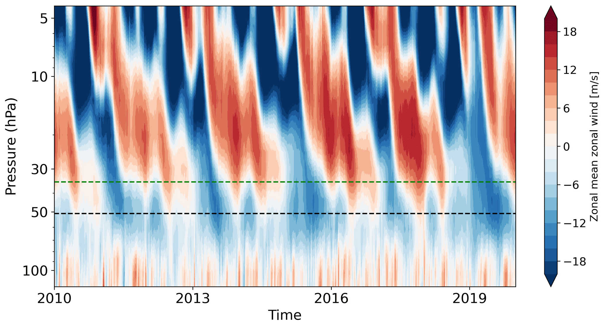
Figure 1The equatorial (5∘ S–5∘ N) zonal-mean zonal winds from 2010–2020 based on the present-day climate of the GLENS simulation.
Here all 20 ensemble members of the GLENS simulations are used to represent the PDC (2010–2029) and SAI (2060–2079) simulations. The three available ensemble members from the RCP8.5 (2060–2079) simulation are used. It is worthwhile to mention that in CESM1(WACCM) both orographic and non-orographic (frontal and convectively generated) gravity waves (GWs) are parameterized based on the GW source specification of Richter et al. (2010), with the GW propagation scheme of Lindzen et al. (1981). By increasing the efficiency of convectively generated GWs and increased horizontal resolution compared to Mills et al. (2016), CESM1(WACCM) generates an internal QBO (Mills et al., 2017). The mean period of the simulated QBO ranges from 23 to 27 months for ensemble members. In observations, the mean QBO period is about 28 months and ranges between 20 and 34 months. The amplitude of the simulated westerly QBO phase is comparable to observations. However, the amplitude of the easterly phase is weaker than in observations (Fig. 4a and b of Mills et al., 2017). The simulated QBO is somewhat deficient in the lower stratosphere as the westerly phase does not reach down to about 100 hPa as in observations, but it is confined to above approximately 50 hPa (see Fig. 1). Richter et al. (2022) reported that most CMIP6 models systematically underestimate the amplitude of the lower-stratospheric QBO.
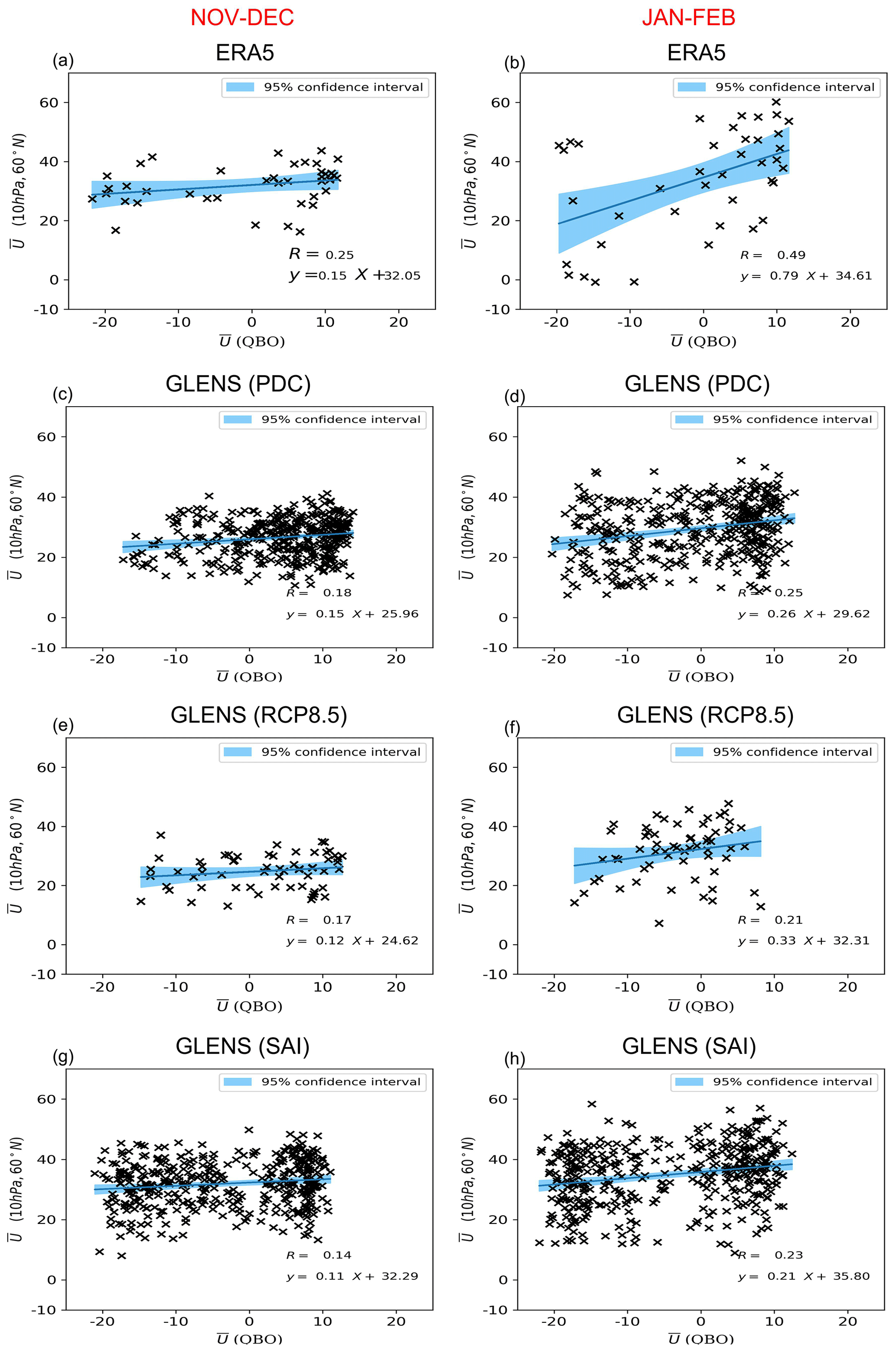
Figure 2Scatter plot of the strength of the stratospheric polar vortex at 10 hPa versus the strength of the equatorial zonal-mean zonal wind in ERA5 (QBO defined at 50 hPa) and GLENS (QBO defined at 35 hPa) simulations. Text in each panel gives the results of an ordinary least squares regression through the points. The shaded areas show the 95 % confidence intervals.
Despite the well-established relationship between the QBO phases and the strength of the Northern Hemisphere (NH) stratospheric polar vortex, it still remains unclear which vertical levels of the QBO exert the strongest influence on the polar vortex. In particular, the following remains an open question: if a deep layer of westerly or easterly equatorial winds influences the high-latitude polar vortex, why is a QBO definition of 50 hPa based on the equatorial zonal-mean zonal wind (Holton and Tan, 1980; Garfinkel et al., 2012) a better choice than other levels (Anstey et al., 2014)? Indexing the QBO at 50 hPa is not feasible in the GLENS simulation due to the weak amplitude of the simulated westerlies there (see Fig. 1). Instead, the closest higher level (level 42, which is at about 35 hPa) is selected to index the QBO where both easterlies and westerlies have large enough amplitudes to detect the QBO phases. The QBO is indexed using the zonally averaged zonal wind between 5∘ S and 5∘ N, as QBOw, and as QBOe. The composite differences of variables are expressed as QBOe minus QBOw. As the strength of the QBO modulation of the planetary waves changes from early winter to late winter (Holton and Tan, 1982; Hu and Tung, 2002), we study the early winter (November–December) and middle to late winter (January–February) responses separately. We use Student's t test at 95 % significance to determine whether two datasets are significantly different. Ideally, the GLENS's historical simulation (1980–2010) might be used to evaluate the model performance in simulating the HT effect (by comparing to ERA5 reanalysis during a similar period). Unfortunately, the historical simulation is a single member and given large variability of the strength of the polar vortex, such evaluation is not reliable (figures not shown). Instead, we use ERA5 reanalysis (Hersbach et al., 2020) for the period 1980–2019 to evaluate the PDC (2010–2029, consisting of 20 ensemble members) for the representation of the QBO modulation of the stratospheric polar vortex in the GLENS simulations.
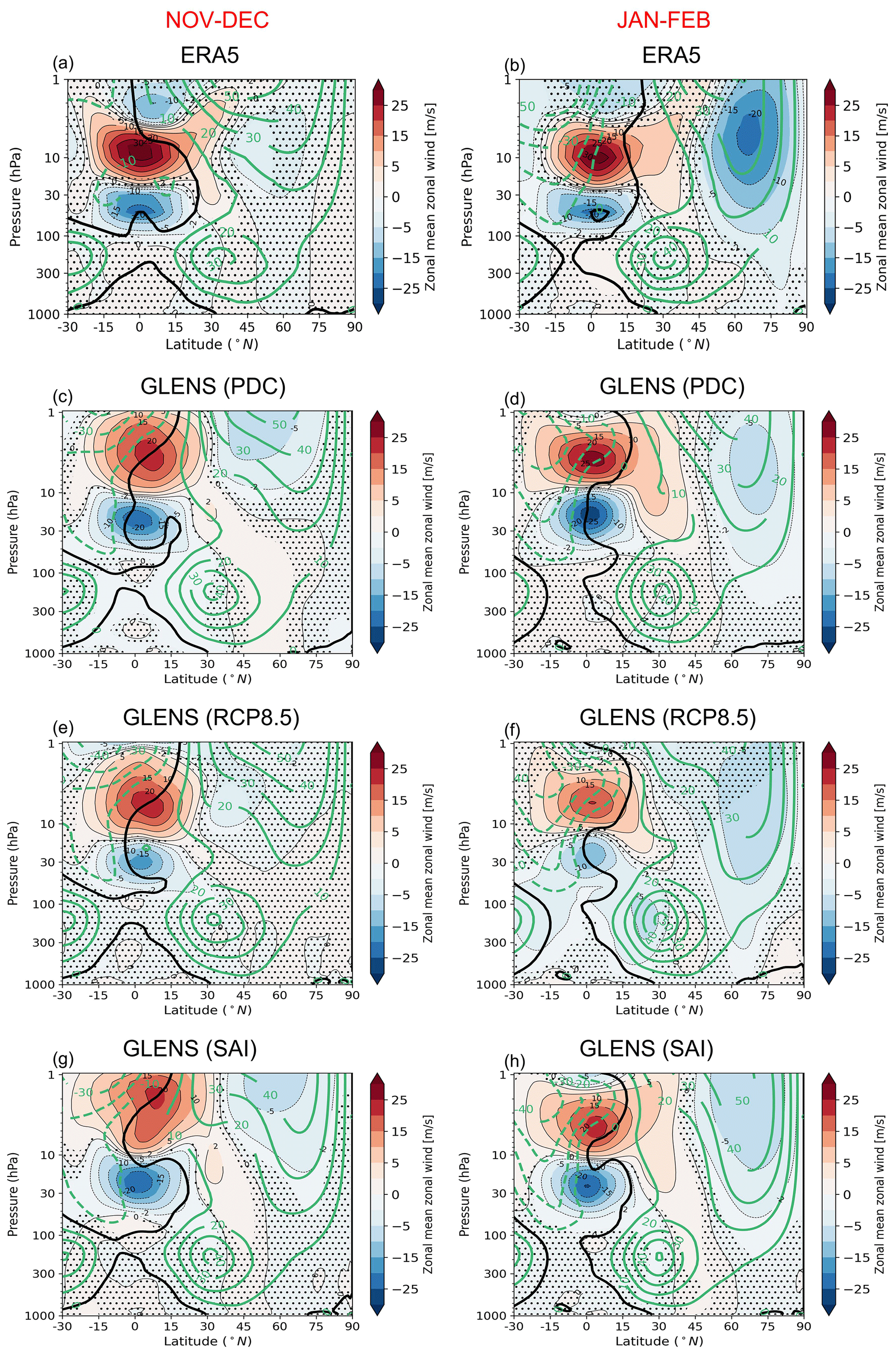
Figure 3Latitude–pressure cross section of the composite differences between QBOe and QBOw (QBOe–QBOw) for November–December (left column) and January–December (right column) of the zonal-mean zonal wind. The stippled areas indicate regions where the changes are not statistically significant at the 95 % level according to the t test. The green contours represent the zonal-mean zonal winds of the respective dataset or simulation.
2.2 Transformed Eulerian mean equation and waveguide metrics
We employ a number of diagnostics, including the Eliassen–Palm (EP) flux and its divergence, the quasi-geostrophic refractive index, and the mean meridional circulation. The dynamical processes can be described based on the transformed Eulerian mean (TEM) momentum equation, which connects the changes in the circulation to wave forcing (Andrews et al., 1987). It can be expressed as
where u, v, and w are Eulerian zonal, meridional, and vertical winds, ϕ is the latitude, a is the Earth's radius, f is the Coriolis parameter, and is the standard density in log-pressure coordinates, where ρs is the reference density at 1000 hPa and H is the scale height (7 km). Subscripts denote derivatives with respect to the given parameter. The first and second terms on the right-hand side (RHS) of Eq. (1) are the acceleration associated with the TEM meridional circulation , where
Here and are the components of the Eulerian mean meridional circulation and θ is the potential temperature.
The third term on the RHS of Eq. (1) is the divergence of the quasi-geostrophic version of the EP flux, which is proportional to the eddy heat and momentum fluxes. The EP flux indicates the strength and direction of large-scale wave propagation. The divergence of the EP flux, which represents the zonal forcing on the mean zonal flow from the large-scale resolved waves, is defined as
where the vertical and meridional components of the EP flux are
and
The last term in Eq. (1) is the forcing by dissipation and other unresolved processes such as gravity wave drags. The stream function of the residual mean meridional circulation can be estimated by the vertical integration of :
Here, we adapt the methodology introduced by Okamoto et al. (2011) to calculate the relative contributions of the resolved Rossby waves versus unresolved zonal force (e.g., gravity wave drag) in driving the mean residual circulation. Their method is based on the downward control principle (DCP) proposed by Haynes et al. (1991), whereby the DCP suggests that the meridional residual flow in the middle atmosphere is largely driven the dissipating waves in the midlatitudes, and the vertical flows are then induced in the tropics and higher latitudes by mass conservation. The DCP also states that in the steady-state case and neglecting the vertical advection by the residual mean flow, the extratropical meridional mass flow at a given pressure level is determined solely by the sum of all zonal forces above the pressure level. Therefore,
where
In pressure coordinates, we have
and
Here, the subscript “direct” is used for the results calculated by Eq. (7), which accounts for both resolved and unresolved wave forcings, the subscripts “epfd” and “gwd” represent the contribution of the zonal forcing by resolved waves and parameterized gravity waves, respectively, and g is the gravitational acceleration.
For the wave guide metric, we use the method of Karami et al. (2016). The probability of favorable propagation conditions for Rossby waves is based on the frequency distribution of days with positive vertical wavenumber squared, which was originally introduced by Matsuno (1970) as a diagnostic tool for studying the influence of the background zonal flow on the large-scale planetary wave (PW) propagation. According to linear wave theory, the PWs tend to propagate to the regions where the vertical wavenumber squared is positive and avoid regions with small or negative values of this quantity. Here we use a two-dimensional (depending on the zonal and meridional wavenumbers) formulation of the vertical wavenumbers (Sun and Li, 2012; Sun et al., 2014):
where
is the meridional gradient of the zonally averaged potential vorticity (Andrews et al., 1987). Here k, l, N2, and ω are the zonal and meridional wavenumbers, buoyancy frequency, and the Earth's angular rotation frequency, respectively. Here we only consider the stationary planetary waves with zero phase speed. It is worthwhile to mention that the index of refraction has different forms. Weinberger et al. (2021) evaluated the ability of four different versions of the index of refraction to capture the upward wave propagation from the troposphere to the stratosphere. In particular, they show that the vertical gradients in buoyancy frequency near the tropopause are critical for understanding the upward wave propagation from the troposphere. In the form of the refractive index used in Eq. (12) the buoyancy frequency varies in the vertical direction and is hence sensitive to its changes near the tropopause and therefore is suitable for the current study.
3.1 Influence of the equatorial QBO on the extratropical circulation
Scatter plots of the QBO zonal mean winds versus the stratospheric polar vortex wind at 10 hPa and 60∘ N are shown in Fig. 2. For ERA5, the equatorial zonal mean wind, , is defined at 50 hPa and for the GLENS simulation at 35 hPa (see Sect. 2); therefore, slightly different responses between the two datasets are expected (note that the periods covered by ERA5 and PDC are also different). Both ERA5 and the PDC simulation of the GLENS project suggest that the strength of the HT relationship is stronger in January–February compared to the November–December period. This also holds true for the RCP8.5 and SAI simulations. The strength of the HT relationship in SAI is weaker compared to the PDC of GLENS simulation. While in November–December the HT relationship is also weaker in the RCP8.5 compared to the PDC, the relationship is stronger in the January–February period. Richter et al. (2018) showed that the period and the amplitude of the QBO are affected by both global warming and SAI. They showed that the mean QBO period decreases to 14 months by the end of the century (2080–2099) under the RCP8.5 scenario compared to 24 months in 1980–1999. They attributed the shortening of the QBO period under the RCP8.5 scenario of the GLENS simulation to an enhancement of the amplitude of tropical convective heating that increases the gravity wave momentum flux entering the stratosphere. In the SAI simulation, the mean period also decreases to about 21 months in 2080–2099, but it remains closer to what is simulated than in the RCP8.5 simulation. The reason is that in the SAI simulation the sea surface temperatures, and hence the strength of convection, remain close to 2020 levels, and therefore the gravity wave momentum entering the stratosphere remains at those levels such that the QBO period does not change significantly. As shown in Fig. 2g and h, the easterlies under SAI dominate the QBOe phase compared to the PDC, and westerlies weaken, which is more pronounced in November–December. This is associated with the change in the climatology of the zonal-mean zonal wind towards a stronger easterly state under the SAI scenario (Tilmes et al., 2018a; Richter et al., 2017).
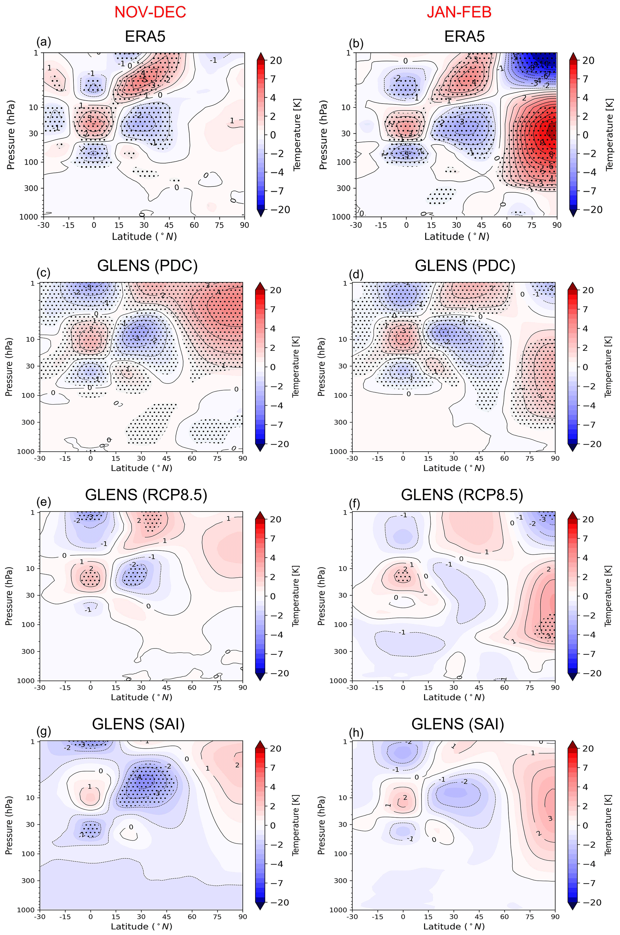
Figures 3 and 4 show the QBO composite differences (QBOe–QBOw) of zonal-mean zonal wind and temperature averages, respectively. In the equatorial region, in both ERA5 and GLENS, the response of is most significant at the pressure levels at which the phase of the QBO was defined for each dataset. In the high-latitude stratosphere, the weakening of and correspondingly warmer polar region mark the HT effect. While the PDC of the GLENS simulation underestimates the HT relationship compared to ERA5 in January–February, a stronger HT relationship is found in November–December. Nevertheless, despite the differences between the PDC of the GLENS simulation and ERA5 reanalysis, the pattern of the HT relationship is reasonably represented in the PDC of the GLENS simulations. Both ERA5 and GLENS PDC agree on the larger areal extent of the HT effect in the early winter (November–December). The well-known, three-vertical-cell structure of the temperature anomalies is evident both at the Equator and in the subtropics in all datasets. The structure is geostrophically consistent with the wind structure (Fig. 3) and is maintained by adiabatic cooling and warming associated with the secondary meridional circulation of the QBO (Plumb and Bell, 1982); this will be discussed further in the next section.
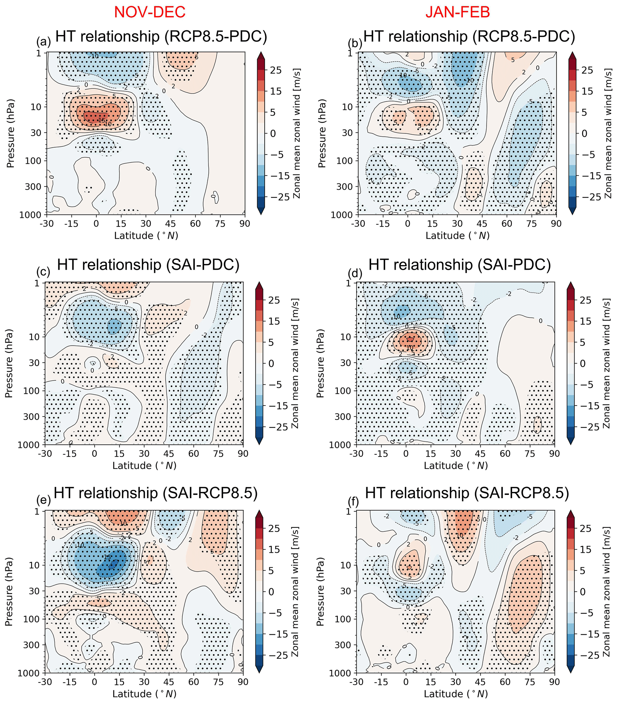
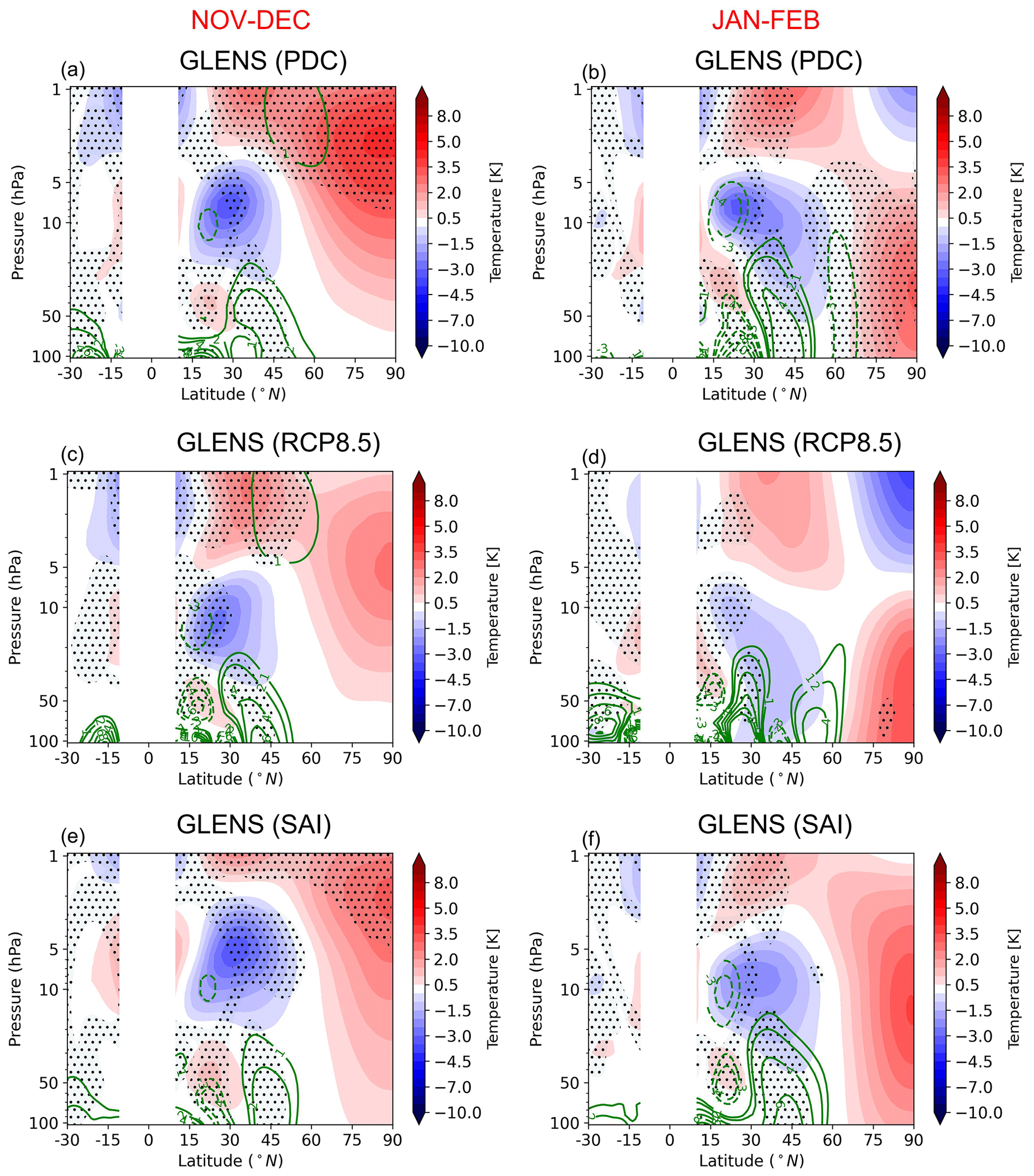
Figure 5Changes in the HT relationship (for zonal-mean zonal wind) under SAI and global warming (RCP8.5) scenarios compared to the PDC.
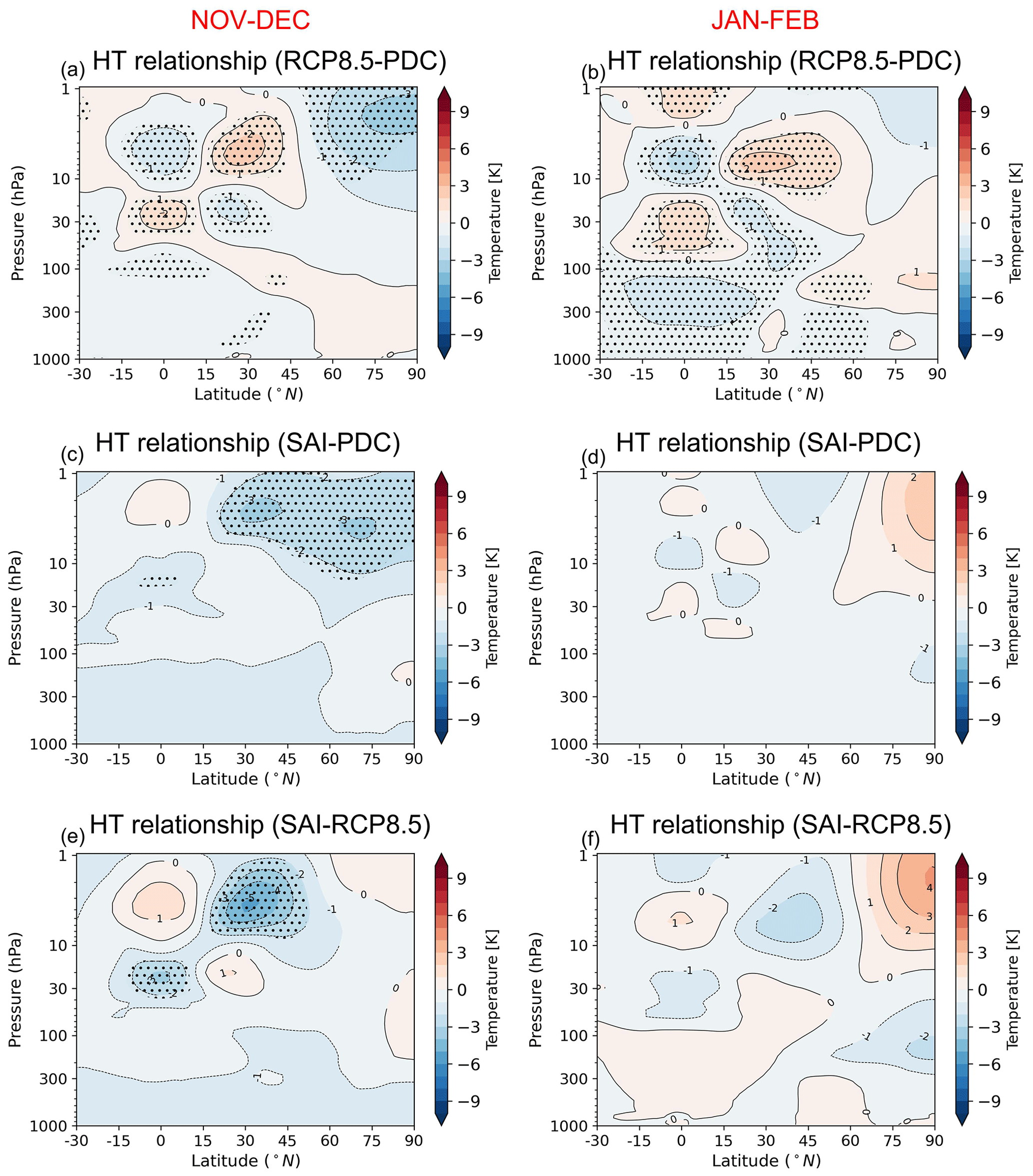
To examine the changes in the HT relationship between the SAI and RCP8.5 scenarios compared to the PDC simulation, Figs. 5 and 6 respectively show the composite differences of the zonal-mean zonal wind and temperature responses due to the HT relationship (presented in Figs. 3 and 4). In RCP8.5, the QBO central anomaly at 35 hPa is not only weaker than in PDC, but its vertical and meridional extent also covers a smaller area. In the SAI simulation the QBO central anomaly also weakens slightly compared to PDC, but it remains closer in both magnitude and vertical extent of the anomalies to what is simulated under PDC than in the RCP8.5 simulation. The positive (negative) zonal-mean zonal wind (Fig. 5a–d) and negative (positive) temperature (Fig. 6a–d) anomalies in the high-latitude stratosphere indicate a weaker (enhanced) HT relationship under either the RCP8.5 or SAI scenario compared to the PDC. While the high-latitude responses of temperature to the QBO anomalies are statistically significant in PDC, they are not significant under the RCP8.5 and SAI scenarios (Fig. 4). The weakened HT relationship in November–December under the SAI scenario cannot be attributed to the changes in the QBO anomalies in the equatorial region, as it largely resembles the QBO anomalies under the PDC simulation. However, under a warming climate (RCP8.5 simulation) it is more likely that the changes in the HT relationship are due to the smaller magnitude of the QBO anomalies in the equatorial region (Fig. 3e and f) compared to the SAI.
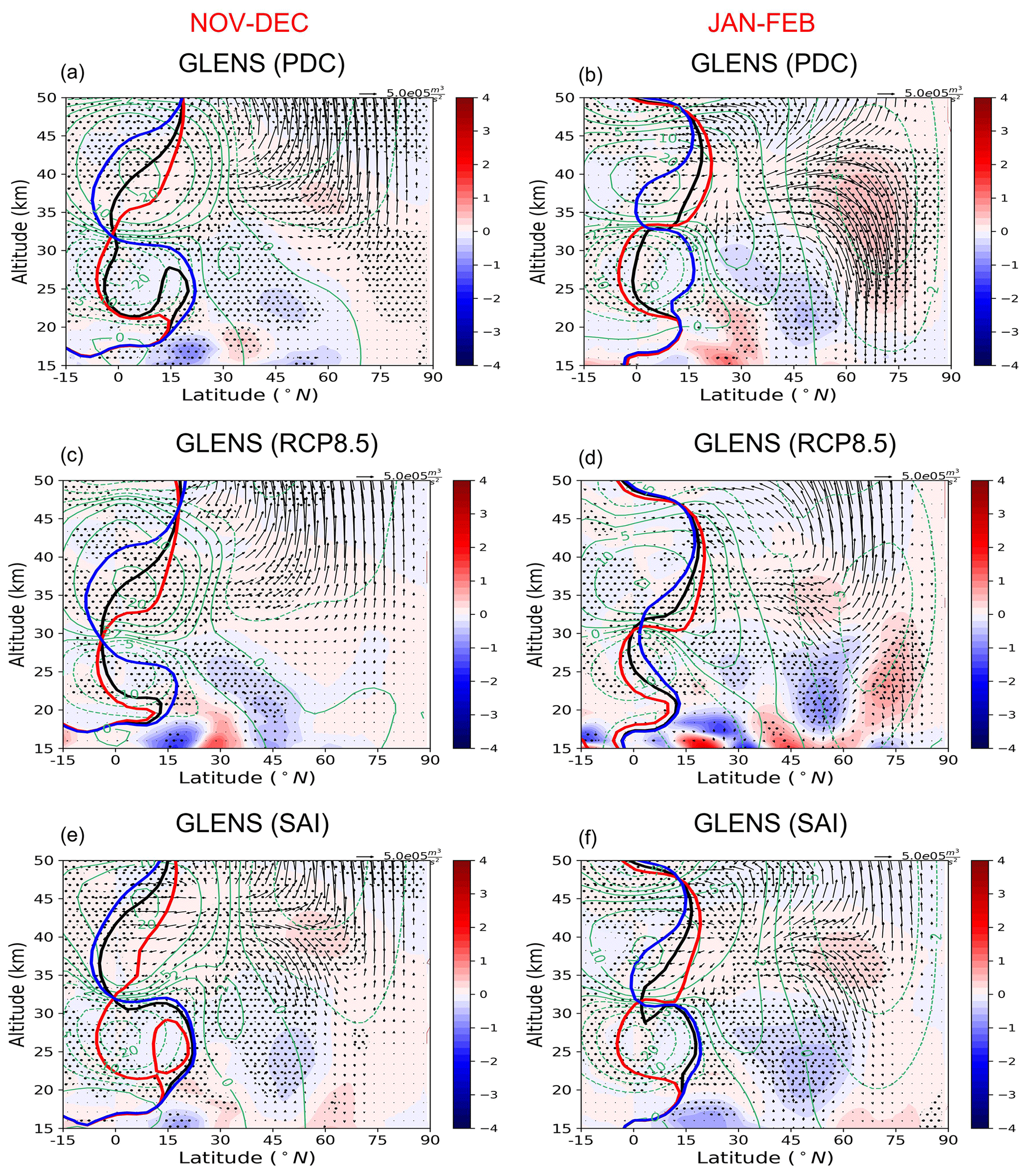
Figure 7Latitude–height cross section of the QBOe–QBOw composite differences of the EP flux (arrows) and its divergence (color shaded in m s−1 d−1). The green contours are the zonal-mean zonal wind responses, and the solid red, blue, and black lines are the locations of the zero-wind line for the QBOw, QBOe, and climatology, respectively. The stippled areas indicate regions where the changes in the EP flux divergence are statistically significant at the 95 % level according to the t test.
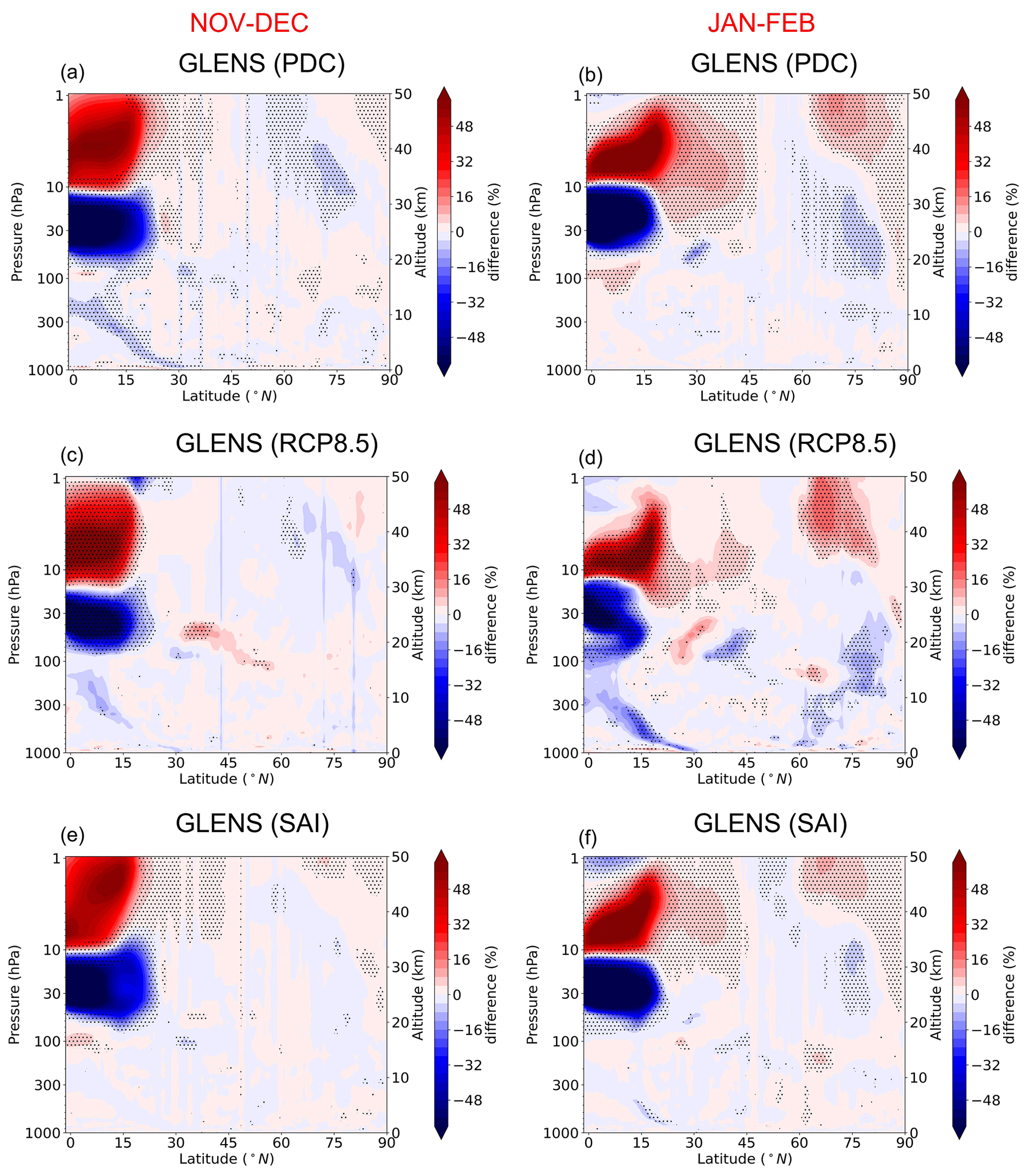
Figure 8Latitude–pressure cross section of the QBOe–QBOw composite differences in percentages of the favorable propagation condition for the resolved large-scale waves (based on the refractive index of Rossby waves). The stippled areas indicate regions where the changes in the quantity are statistically significant at the 95 % level according to the t test.
Figure 7 shows the composite QBOe–QBOw differences of the EP flux, its divergence, the zonal-mean zonal wind response, and the location of the zero-wind line for the different QBO phases. We found that under QBOe the climatologically equatorward component of the EP flux is weaker than under QBOw, and hence the composite differences show that under different climate change scenarios the resolved waves are always directed towards the high latitudes in the middle and upper stratosphere. At first glance, this might seem consistent with the traditional HT hypothesis (Holton and Tan, 1980) that under QBOe, the quasi-stationary waves cannot propagate in easterly winds and therefore the effective waveguide for the planetary waves is narrower compared to the QBOw case. However, these regions are generally well above the region of easterlies and are above 30 km where westerlies prevail. This is shown in Fig. 8 as the positive anomaly of the favorable propagation condition for Rossby waves between 10 and 1 hPa, which is a pattern that is generally found in all scenarios. While the zero-wind line is on the winter side of the Equator (20–30 km) for QBOe under the PDC and SAI scenarios, the distance between the location of the zero-wind line is smaller for the different QBO phases under RCP8.5 (particularly in January–February). This is also reflected in Fig. 8 where the anomalies of the favorable propagation condition for Rossby waves are meridionally limited and also weaker under RCP8.5 compared to the SAI and PDC simulations, particularly in January–February. This is also expected as the zonal-mean zonal wind anomalies (Fig. 3) show similar patterns. While the weaker equatorward EP flux component in QBOe–QBOw composites is a persistent feature in all scenarios and periods, the vertical EP flux component shows inconsistent responses. In general, in early winter (November–December) an enhanced upward EP flux is found in the high-latitude stratosphere in all scenarios. On the other hand, in middle to late winter (January–February) a reduction of the upward EP flux is found in all scenarios. Although the polar vortex is modulated as expected (see Figs. 3 and 4), the wave propagation does not follow the HT mechanism, which is in agreement with the study of Naoe and Shibata (2010) and Yamashita et al. (2011). This suggests that the effect of the zero-wind line emphasized in the HT mechanism is not so important in the QBO modulation of the wintertime stratospheric polar vortex.
Alternatively, Garfinkel et al. (2012), by performing idealized experiments using WACCM, reported that the subtropical critical line modulates the synoptic Rossby wave convergence in the subtropical lower stratosphere and cannot directly influence the large-scale waves in the middle and higher latitudes. Instead, they suggest that the secondary meridional circulation of the QBO, which modifies the zonal mean wind distribution, affects the refractive index and this influences the wave propagation in the middle and higher latitudes of the upper stratosphere. It is also worthwhile to mention that it is challenging to isolate the exact mechanism(s) by which the QBO influences the vortex in the comprehensive general circulation models (GCMs) such as our dataset due to the presence of unrelated variability. For example, variability in sea surface temperature (SST) not only influences the tropospheric planetary wave activity (Garfinkel and Hartmann, 2008; Hurwitz et al., 2011) but also affects the strength of the HT mechanism (Holton and Austin, 1991; O'Sullivan and Dunkerton, 1994). The signs of the refractive index and EP flux in our analysis are somewhat different than those reported by Garfinkel et al. (2012), likely due to the more idealized experiments in Garfinkel et al. (2012) with fixed SSTs, land surface and ice, and perpetual midwinter radiative forcing, as well as the lack of interactive chemistry that might mask the HT mechanism (Wei et al., 2007; Garfinkel and Hartmann, 2007; Calvo et al., 2009); nevertheless, we will show that the high-latitude modulation of the polar vortex in different scenarios can be explained by the changes in the residual circulation, consistent with the study of Garfinkel et al. (2012).
Because the QBO modulation of upward-propagating planetary waves changes from early winter to late winter and also because of a lack of persistence in the wave response, we suggest that the critical line mechanism is not the sole mechanism for changes in the HT relationship in the GLENS simulations. Similar to our results, previous researchers (Dunkerton and Baldwin, 1991; Ruzmaikin et al., 2005; Naoe and Shibata, 2010; Yamashita et al., 2011) have documented changes in planetary wave amplitude and/or EP flux and EP flux convergence that are inconsistent with what one would expect from the HT relationship. This is likely because it is not straightforward to predict the influence of the subtropical critical line in reflecting planetary waves, in particular due to the feedback processes that are initiated as a result of the wave forcing (Watson and Gray, 2014).
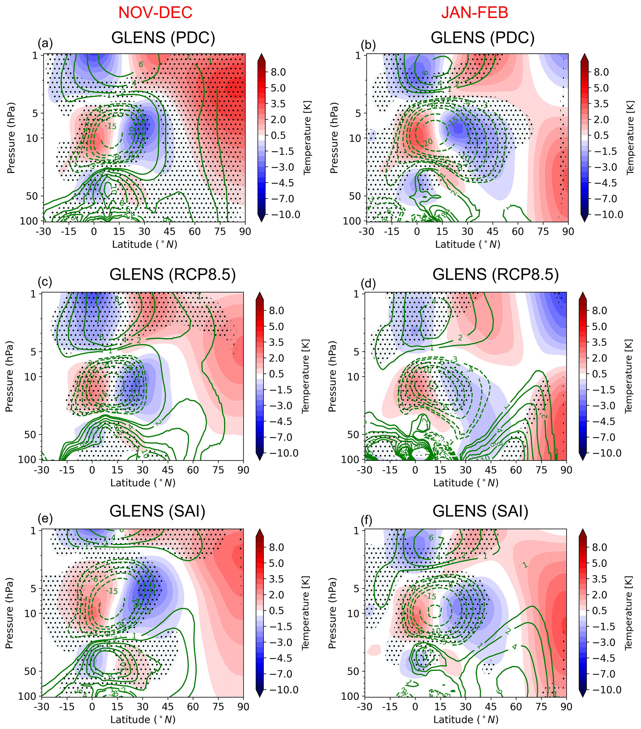
Figure 9Latitude–pressure cross section of the QBO composite differences (QBOe–QBOw) of the zonal mean meridional stream lines (green contours) and temperature (color shaded). The streamlines are calculated based on Eq. (7), and hence the contributions from both Rossby and gravity waves are included. The stippled areas indicate regions where the changes in the zonal mean meridional stream lines are statistically significant at the 95 % level according to the t test.
Figure 9 shows the QBOe–QBOw composite differences in the zonal mean meridional stream lines and zonal mean temperature responses. The positive and negative anomalies of the stream lines indicate clockwise and anticlockwise circulation, respectively. The QBO induces a three-vertical-cell structure of the temperature anomalies both at the Equator (10∘ S–10∘ N) and in the subtropics (10–40∘ N in November–December and 10–50∘ N in January–February) in all scenarios and periods. This circulation, known as the secondary meridional circulation, is characterized by sinking motion anomalies at the Equator (10∘ S–10∘ N) in westerly shear zones and a rising motion in easterly shear zones. In the tropics, the temperature has a thermal wind relationship with the vertical shear of zonal wind such that QBO-induced cold and warm temperature anomalies coincide with easterly and westerly shear zones, respectively (Plumb and Bell, 1982; Randel et al., 1999; Ribera et al., 2004). The QBO-induced temperature anomaly changes sign at approximately . The temperature anomalies in the subtropics are out of phase compared to the equatorial anomalies as they are related to the return branches of the secondary meridional circulation induced by the QBO. The area of the subtropical temperature anomalies is larger than its tropical counterpart, and they often extend to the midlatitude winter hemisphere (Kinnersley and Tung, 1998). The latitudinal extension of the temperature meridional cells to midlatitudes occurs via modulation of the extratropical Rossby waves (Ribera et al., 2004; Baldwin et al., 2001; Kinnersley and Tung, 1998). The temperature anomalies at high latitudes correspond well to the changes in the mean meridional circulation. In particular, it is found that in QBOe–QBOw composites (Fig. 9), the streamline anomalies are positive, indicating a clockwise circulation and hence sinking in the high latitudes; thus, under QBOe the climatological sinking is enhanced compared to the QBOw, which is in agreement with the composites of temperature. Figure 9 also shows that the QBO-induced anomalies of the zonal mean meridional circulation at high latitudes in November–December are not significant under RCP8.5 and SAI simulations, while they are large and statistically significant in the PDC simulation. This clearly explains the weaker temperature responses under the RCP8.5 and SAI simulations compared to the PDC. Therefore, it can be concluded that the weaker clockwise circulation anomalies in the high-latitude stratosphere in the QBOe–QBOw composites under RCP8.5 and SAI scenarios compared to the PDC simulation in November–December are the primary reason for the weakening of the HT relationship in RCP8.5 and SAI scenarios, and the subtropical zero-wind line plays a less important role.
Figures 10 and 11 show the QBOe–QBOw composite differences of the contributions from the resolved Rossby waves and unresolved gravity waves in driving the mean meridional circulation anomalies. In general, the magnitudes of the composite differences are larger for the gravity waves. Particularly in the high latitudes, the composite differences of the zonal mean meridional circulation due to the gravity waves explain the temperature responses well. It is also found that the resolved waves contribute minimally to the QBOe–QBOw composite differences in temperature in low latitudes. Instead, the contribution from the unresolved gravity waves is very robust in these regions. In the subtropics and midlatitude regions, the contribution from the Rossby waves is also considerable. It is worthwhile to mention that gravity waves have a climatologically counterclockwise circulation in region between 45 and 75∘ N (see Fig. 3c of Okamoto et al., 2011). Therefore, the positive anomalies in these regions indicate a weakening of the counterclockwise circulation by the gravity wave dissipations under QBOe compared to QBOw. The arched down (downward extension) temperature anomalies towards the tropopause in the midlatitudes are due to the contribution of both Rossby and gravity waves. In November–December, the composite differences of the residual circulation due to gravity waves extend to high latitudes and are statistically significant only for PDC, but that is not the case for the RCP8.5 and SAI simulations and this explains the weaker HT relationship under RCP8.5 and SAI compared to the PDC. In January–February, the composite differences of QBOe–QBOw of the residual circulation are enhanced in the RCP8.5 and SAI in the middle and high latitudes, which is due to the gravity wave contribution.
We examined changes in the HT relationship under a strategic SAI scenario and a scenario with high anthropogenic emissions (RCP8.5) and compared them to the present-day climate (PDC) by using century-long GLENS project simulations. While the PDC underestimates the HT relationship compared to ERA5 in January–February, a stronger HT relationship is found in November–December. Nevertheless, the pattern of the HT relationship is reasonably represented in the PDC, suggesting that the model configuration is suitable for investigation of the possible future changes. The composite differences (QBOe–QBOw) of zonal wind and temperature show that the HT relationship weakens under both the RCP8.5 and SAI scenarios in November–December, although the HT relationship remains closer to PDC under SAI than under RCP8.5. In January–February, the HT relationship does not change considerably in response to either the RCP8.5 or SAI scenario compared to PDC. While the different phases of the equatorial QBO cause statistically significant temperature changes in the high-latitude stratosphere under PDC, the responses are not statistically significant in the RCP8.5 and SAI scenarios. It is worthwhile to mention that the HT relationship in this study only refers to the teleconnection between the QBO and the Arctic stratospheric polar vortex, and other aspects of QBO influence such as surface impacts are not studied in this paper. One reason is that investigating the surface influence of the QBO via the stratospheric polar vortex path requires a model with high vertical resolution. WACCM6, with a relatively coarse vertical resolution of 70 layers between the surface and model top at 140 km, is not useful for such an investigation.
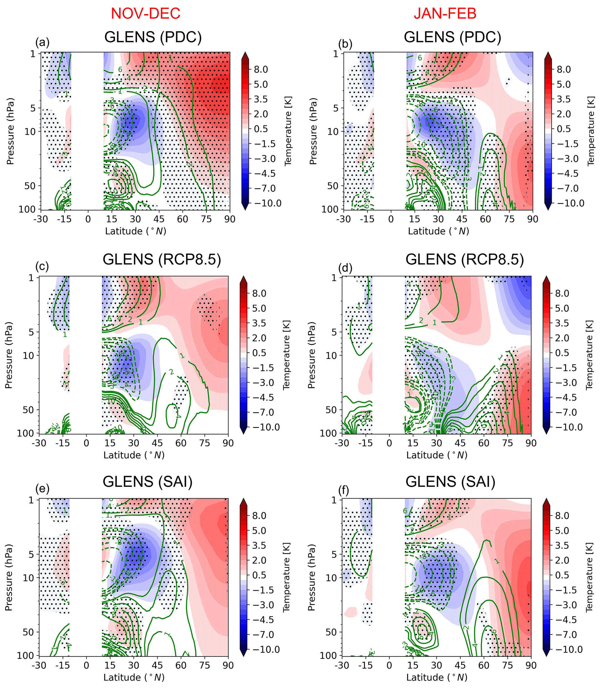
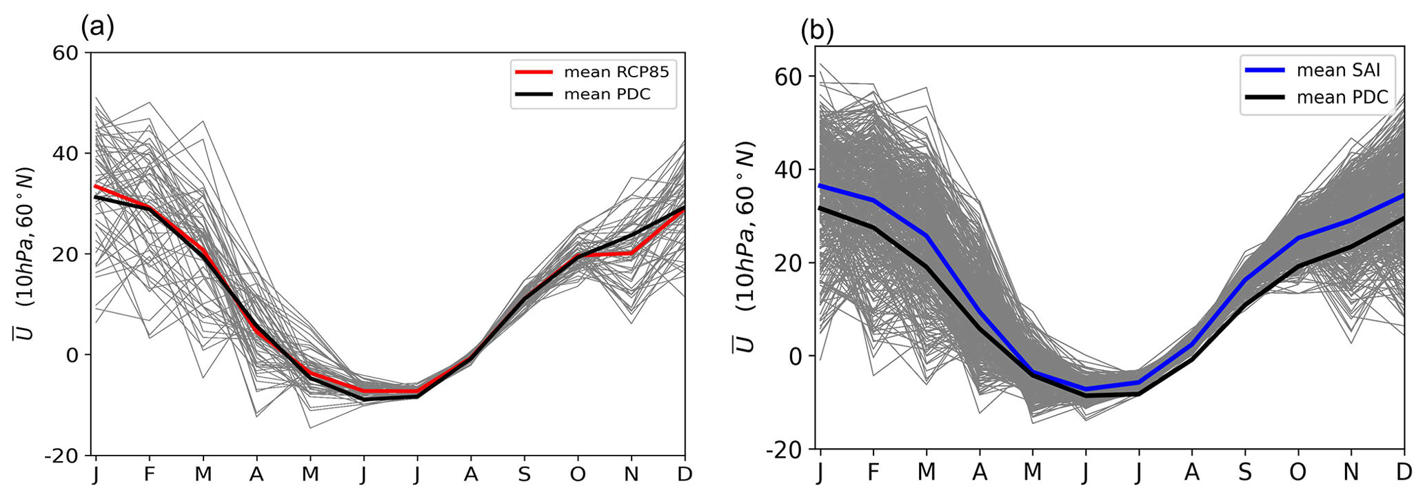
Figure 12Monthly mean evolution of the zonal-mean zonal wind at 10 hPa and 60∘ N for the RCP8.5 (a) and SAI (b) simulations. The zonal winds for each year for the RCP8.5 and SAI scenarios are shown by the gray lines, and the multi-ensemble multi-year averages are shown by the red and blue lines for RCP8.5 and SAI, respectively. The black line indicates the multi-ensemble multi-year average of the PDC simulation.
The central anomaly of QBO at 35 hPa is weaker and its vertical and meridional extents are limited under RCP8.5 compared to PDC. This is also reflected in the location of the zero-wind line (critical level): the distance between the location of the zero-wind line is shorter for the different QBO phases under RCP8.5 (particularly in January–February) compared to SAI and PDC. However, the QBO amplitude under SAI remains comparable to PDC. A weaker amplitude of the QBO under RCP8.5 compared to PDC and SAI also weakly influences the effective waveguide of Rossby waves under different phases of QBO such that the wave mean flow interactions largely differ under RCP8.5 compared to PDC and SAI, which resemble each other.
In general, the temperature responses at high latitudes correspond well to the changes in the mean meridional circulation. Our results also show that in November–December the QBO-induced anomalies of the mean meridional circulation at high latitudes are not statistically significant under the RCP8.5 and SAI scenarios, while they are statistically significant under PDC. Further analysis reveals that the gravity wave contribution to composite differences of QBOe–QBOw in November–December are statistically significant under PDC, but this is not the case in RCP8.5 and SAI scenarios. This explains the weaker HT relationship under RCP8.5 and SAI compared to PDC in November–December. In January–February, while the composite differences of QBOe–QBOw of the residual circulation are stronger in RCP8.5 and SAI compared to the PDC (particularly in the middle and high latitudes), the strength of the HT relationship does not considerably change under either scenario compared to the PDC. Therefore, we seek an alternative explanation for the unchanged HT relationship in January–February under both RCP8.5 and SAI scenarios. Richter et al. (2018) reported a reduction in the future frequency of sudden stratospheric warmings (SSWs) in both RCP8.5 and SAI scenarios. The frequency of SSWs between 1975 and 2015 was 0.7 yr−1 and it decreased to 0.36 and 0.28 events per year in RCP8.5 and SAI scenarios, respectively, for the period 2060–2099. They also reported that the polar vortex variability does not change significantly under the RCP8.5 global warming scenario compared to the present-day climate, but the vortex became more stable under the SAI scenario. However, their results were based on a single realization of the RCP8.5 and SAI scenarios. Figure 12 shows the monthly mean evolution of the zonal-mean zonal wind at 10 hPa and 60∘ N for both RCP8.5 and SAI scenarios based on all ensemble members of GLENS (20 members for the PDC and SAI and 3 members for the RCP8.5). The average change in the zonal-mean zonal wind at 10 hPa and 60∘ N for the cold season (October–March) is 0.11 m s−1 for the RCP8.5 scenario and 5.75 m s−1 for the SAI scenario. Here we suggest that the unchanged HT relationship under the SAI scenario in January–February might be related to the more stable polar vortex (and hence colder polar stratosphere) under SAI compared to the PDC.
Table 1The relative composite differences (QBOe–QBOw) of different physical mechanisms influencing the strength of the HT relationship in November–December. The weaker and stronger mechanisms are relative to the PDC. A blank indicates insignificant changes compared to the PDC.
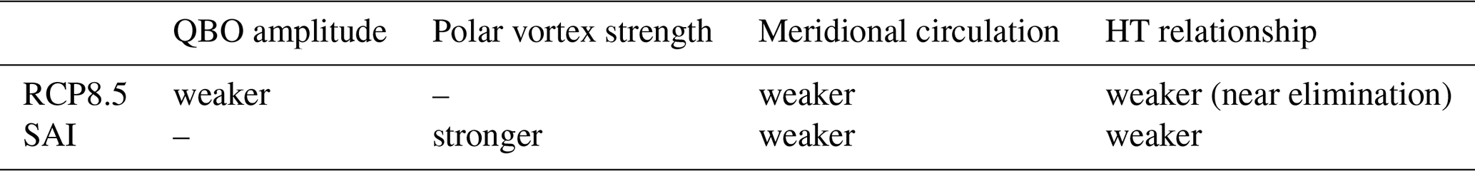
Table 2The same as Table 1 but for the January–February period.
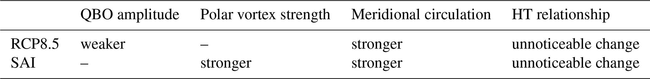
Although it is difficult to fully disentangle the contributing factors to the changes in the HT relationship under different climate change scenarios, Tables 1 and 2 summarize the relative roles of different physical mechanisms in influencing the changes in the HT relationship under the RCP8.5 and SAI scenarios compared to the PDC. The changes in the HT relationship under the RCP8.5 might be explained by the weaker QBO amplitudes (e.g., the weaker QBO amplitudes have weaker potential to influence the high latitudes). However, under the SAI scenario the QBO amplitudes do not significantly differ compared to the PDC, but the polar vortex accelerates and we attribute the weakening of the HT relationship under the SAI scenario to the more stable polar vortex. Another relevant point in the interpretation of the QBO composite differences of the zonal mean meridional stream lines due to the resolved and unresolved waves is the so-called compensation mechanism, whereby the changes in the gravity wave forcing are compensated for by the resolved wave driving of opposite sign (Cohen et al., 2001; Sigmond and Shepherd, 2014; Garcia et al., 2017; Eichinger et al., 2020).
Finally, we would like to mention that the results presented here are based on relatively coarse-vertical-resolution simulations (70 L model), which have a somewhat deficient QBO. It is important to investigate the robustness of these findings with a higher-vertical-resolution version of CESM1(WACCM) to gain additional confidence in our results. In addition, examining the changes in the HT relationship under the SAI scenario using other Earth system models would be useful due to uncertainties inherent in complex Earth system models.
NCAR's GLENS simulation datasets can be downloaded here: https://www.cesm.ucar.edu/projects/community-projects/GLENS/ (National Center for Atmospheric Research, 2023).
The figures are produced by KK. ST led and JHR contributed to the GLENS simulation. All co-authors contributed to writing and interpreting the results.
The contact author has declared that none of the authors has any competing interests.
Publisher's note: Copernicus Publications remains neutral with regard to jurisdictional claims in published maps and institutional affiliations.
This article is part of the special issue “Resolving uncertainties in solar geoengineering through multi-model and large-ensemble simulations (ACP/ESD inter-journal SI)”. It is not associated with a conference.
This material is based upon work supported by the National Center for Atmospheric Research, which is a major facility sponsored by the National Science Foundation under cooperative agreement no. 1852977. The Community Earth System Model (CESM) project is supported primarily by the National Science Foundation. This study is funded by the Deutsche Forschungsgemeinschaft (DFG) under grant number JA 836/47-1 and within the Transregional Collaborative Research Centre SFB/TRR 172 (project-ID 268020496), subproject D01. This work used resources of the Deutsches Klimarechenzentrum (DKRZ) granted by its Scientific Steering Committee (WLA) under project ID bb1238.
This study is funded by the Deutsche Forschungsgemeinschaft (DFG) under grant numbers JA 836/43 and JA 836/47-1, as well as within the Transregional Collaborative Research Centre SFB/TRR 172 (project ID 268020496), subproject D01, and the National Center for Atmospheric Research (grant no. 1852977).
This paper was edited by Hailong Wang and reviewed by two anonymous referees.
Andrews, M. B., Knight, J. R., Scaife, A. A., Lu, Y., Wu, T., Gray, L. J., and Schenzinger, V.: Observed and simulated teleconnections between the stratospheric quasi-biennial oscillation and northern hemisphere winter atmospheric circulation, J. Geophys. Res.-Atmos., 124, 1219–1232, 2019. a
Andrews, D., Holton, J., and Leovy, C. B.: Middle atmosphere dynamics, Academic press, ISBN: 9780120585762, 1987. a, b
Anstey, J. A. and Shepherd, T. G.: High-latitude influence of the quasi-biennial oscillation, Q. J. Roy. Meteorol. Soc., 140, 1–21, 2014. a
Baldwin, M., Gray, L., Dunkerton, T., Hamilton, K., Haynes, P., Randel, W. J., Holton, J. R., Alexander, M. J., Hirota, I., Horinouchi, T., Jones, D. B. A., Kinnersley, J. S., Marquardt, C., Sato, K., and Takahashi, M.: The quasi-biennial oscillation, Rev. Geophys., 39, 179–229, 2001. a, b
Butler, A., Charlton-Perez, A., Domeisen, D. I., Garfinkel, C., Gerber, E. P., Hitchcock, P., Karpechko, A. Y., et al.: Sub-seasonal predictability and the stratosphere, Sub-seasonal to seasonal prediction, Elsevier, 223–241, ISBN: 9780128117149, https://doi.org/10.1016/B978-0-12-811714-9.00011-5, 2019. a
Cohen, N. Y., Gerber, O., and Bühler, E. P.: Compensation between resolved and unresolved wave driving in the strato sphere: Implications for downward control, J. Atmos. Sci., 70, 3780–3798, 2013. a
Collimore, C. C., Martin, D. W., Hitchman, M. H., Huesmann, A., and Waliser, D. E.: On the relationship between the qbo and tropical deep convection, J. Clim., 16, 2552–2568, 2003. a
Crutzen, P. J.: Albedo enhancement by stratospheric sulfur injections: a contribution to resolve a policy dilemma?, Climatic Change, 77, 211–219, https://doi.org/10.1007/s10584-006-9101-y, 2006. a
Dunkerton, T. J. and Baldwin, M. P.: Quasi-biennial modulation of planetary-wave fluxes in the northern hemisphere winter, J. Atmos. Sci., 48, 1043–1061, 1991. a
Eichinger, R., Garny, H., Šácha, P., Danker, J., Dietmüller, S., and Oberländer-Hayn, S.: Effects of missing gravity waves on stratospheric dynamics, part 1: climatology, Clim. Dynam., 54, 3165–3183, 2020. a
Elsbury, D., Peings, Y., and Magnusdottir, G.: Cmip6 models underestimate the holton-tan effect, Geophys. Res. Lett., 48, e2021GL094083, https://doi.org/10.1029/2021GL094083, 2021. a
Ferraro, A. J., Highwood, E. J., and Charlton-Perez, A. J.: Stratospheric heating by potential geoengineering aerosols, Geophys. Res. Lett., 38, L24706, https://doi.org/10.1029/2011GL049761, 2011. a
Ferraro, A. J., Charlton-Perez, A. J., and Highwood, E. J.: Stratospheric dynamics and midlatitude jets under geoengineering with space mirrors and sulfate and titania aerosols, J. Geophys. Res.-Atmos., 120, 414–429, 2015. a
Hansen, F., Matthes, K., and Gray, L.: Sensitivity of stratospheric dynamics and chemistry to qbo nudging width in the chemistry–climate model waccm, J. Geophys. Res.-Atmos., 118, 464–474, https://doi.org/10.1002/jgrd.50812, 2013. a
Haynes, P., McIntyre, M., Shepherd, T., Marks, C., and Shine, K. P.: On the “downward control” of extratropical diabatic circulations by eddy-induced mean zonal forces, J. Atmos. Sci., 48, 651–678, 1991. a
Hersbach, H., Bell, B., Berrisford, P., Hirahara, S., Horányi, A., Muñoz-Sabater, J., Nicolas, J., Peubey, C., Radu, R., Schepers, D., Simmons, A., Soci, C., Abdalla, S., Abellan, X., Balsamo, G., Bechtold, P., Biavati, G., Bidlot, J., Bonavita, M., De Chiara, G., Dahlgren, P., Dee, D., Diamantakis, M., Dragani, R., Flemming, J., Forbes, R., Fuentes, M., Geer, A., Haimberger, L., Healy, S., Hogan, R. J., Hólm, E., Janisková, M., Keeley, S., Laloyaux, P., Lopez, P., Lupu, C., Radnoti, G., de Rosnay, P., Rozum, I., Vamborg, F., Villaume, S., and Thépaut, J.-N.: The era5 global reanalysis, Q. J. Roy. Meteorol. Soc., 146, 1999–2049, 2020. a
Holton, J. R. and Tan, H.-C.: The influence of the equatorial quasi-biennial oscillation on the global circulation at 50 mb, J. Atmos. Sci., 37, 2200–2208, 1980. a, b, c, d
Holton, J. R. and Tan, H.-C.: The quasi-biennial oscillation in the northern hemisphere lower stratosphere, J. Meteorol. Soc. Jpn. Ser. II, 60, 140–148, 1982. a, b
Holton, J. R. and Austin, J.: The influence of the equatorial QBO on sudden stratospheric warmings, J. Atmos. Sci., 48, 607–618, 1991. a
Hu, Y. and Tung, K. K.: Tropospheric and equatorial influences on planetary-wave amplitude in the stratosphere, Geophys. Res. Lett., 29, 1–4, 2002. a
Hurwitz, M. M., Newman, P. A., and Garfinkel, C. I.: The Arctic vortex in March 2011: A dynamical perspective, Atmos. Chem. Phys., 11, 11447–11453, https://doi.org/10.5194/acp-11-11447-2011, 2011. a
Garcia, R. R., Smith, A. K., Kinnison, D. E., de la Cámara, Á., and Murphy, D. J.: Modification of the gravity wave parameterization in the Whole Atmosphere Community Climate Model: Motivation and results, J. Atmos. Sci., 74, 275–291, 2017. a
Garfinkel, C. I. and D. L. Hartmann, 2007: Effects of the El Niño – Southern Oscillation and the quasi-biennial oscillation on polar temperatures in the stratosphere, J. Geophys. Res., 112, D19112, https://doi.org/10.1029/2007JD008481, 2007. a
Calvo, N., Giorgetta, M. A., Garcia-Herrera, R., and Manzini, E.2009: Nonlinearity of the combined warm ENSO and QBO effects on the Northern Hemisphere polar vortex in MAECHAM5 simulations, J. Geophys. Res., 114, D13109, https://doi.org/10.1029/2008JD011445, 2009. a
Garfinkel, C. and Hartmann, D.: Different enso teleconnections and their effects on the stratospheric polar vortex, J. Geophys. Res.-Atmos., 113, D18114, https://doi.org/10.1029/2008JD009920, 2008. a, b
Garfinkel, C. I., Shaw, T. A., Hartmann, D. L., and Waugh, D. W.: Does the holton–tan mechanism explain how the quasi-biennial oscillation modulates the arctic polar vortex?, J. Atmos. Sci., 69, 1713–1733, 2012. a, b, c, d, e, f
Inoue, M., Takahashi, M., and Naoe, H.: Relationship between the stratospheric quasi-biennial oscillation and tropospheric circulation in northern autumn, J. Geophys. Res.-Atmos., 116, D24115, https://doi.org/10.1029/2011JD016040, 2011. a
Irvine, P., Emanuel, K., He, J., Horowitz, L. W., Vecchi, G., and Keith, D.:Halving warming with idealized solar geoengineering moderates key climate, hazards, Nat. Clim. Change, 9, 295–299, 2019. a
IPCC, V.: Global warming of 1.5 ∘C, intergovernmental panel on climate change, IPCC Geneva, Switzerland, Cambridge University Press, 616 pp., https://doi.org/10.1017/9781009157940, 2018. a
Karami, K., Braesicke, P., Sinnhuber, M., and Versick, S.: On the climatological probability of the vertical propagation of stationary planetary waves, Atmos. Chem. Phys., 16, 8447–8460, https://doi.org/10.5194/acp-16-8447-2016, 2016. a
Karami, K., Tilmes, S., Muri, H., and Mousavi, S. V.: Storm track changes in the Middle East and North Africa under stratospheric aerosol geoengineering, Geophys. Res. Lett., 47, e2020GL086954, https://doi.org/10.1029/2020GL086954, 2020. a
Kinnersley, J. S. and Tung, K.-K.: Modeling the global interannual variability of ozone due to the equatorial qbo and to extratropical planetary wave variability, J. Atmos. Sci., 55, 1417–1428, 1998. a, b
Kodera, K.: The solar and equatorial qbo influences on the stratospheric circulation during the early northern-hemisphere winter, Geophys. Res. Lett., 18, 1023–1026, 1991. a
Kravitz, B., Caldeira, K., Boucher, O., Robock, A., Rasch, P. J., Alterskjaer, K., Bou Karam, D., Cole, J. N. S., Curry, C. L., Haywood, J. M., Irvine, P. J., Ji, D., Jones, A., Egill Kristjánsson, J., Lunt, D. J., Moore, J. C., Niemeier, U., Schmidt, H., Schulz, M., Singh, B., Tilmes, S., Watanabe, S., Yang, S., and Yoon, J.-H.: Climate model response from the geoengineering model inter-comparison project (geomip), J. Geophys. Res.-Atmos., 118, 8320–8332, 2013. a
Kravitz, B., MacMartin, D. G., Tilmes, S., Richter, J. H., Mills, M. J., Cheng, W., Dagon, K., Glanville, A. S., Lamarque, J.-F., Simpson, I. R., Tribbia, J., and Vitt, F.: Comparing surface and stratospheric impacts of geoengineering with different SO2 injection strategies, J. Geophys. Res.-Atmos., 124, 7900–7918, 2019. a
Kravitz, B., MacMartin, D. G., Mills, M. J., Richter, J. H., Tilmes, S., Lamarque, J.-F., Tribbia, J. J., and Vitt, F.: First simulations of designing stratospheric sulfate aerosol geoengineering to meet multiple simultaneous climate objectives, J. Geophys. Res.-Atmos., 122, 12–616, 2017. a, b, c
Kravitz, B., MacMartin, D. G., Robock, A., Rasch, P. J., Ricke, K. L., and Cole, J. N.: A multi-model assessment of regional climate disparities caused by solar geoengineering, Environ. Res. Lett., 9, 074013, https://doi.org/10.1088/1748-9326/9/7/074013, 2014. a
Labitzke, K. and Van Loon, H.: Associations between the 11-year solar cycle, the qbo and the atmosphere, part I: the troposphere and stratosphere in the northern hemisphere in winter, J. Atmos. Terr. Phys., 50, 197–206, 1988. a
Lauvset, S. K., Tjiputra, J., and Muri, H.: Climate engineering and the ocean: effects on biogeochemistry and primary production, Biogeosciences, 14, 5675–5691, https://doi.org/10.5194/bg-14-5675-2017, 2017. a
Lindzen, R. S.: Turbulence and stress owing to gravity wave and tidal break-down, J. Geophys. Res.-Ocean., 86, 9707–9714, 1981. a
Lu, H., Baldwin, M. P., Gray, L. J., and Jarvis, M. J.: Decadal-scale changes in the effect of the qbo on the northern stratospheric polar vortex, J. Geophys. Res.-Atmos., 113, D10114, https://doi.org/10.1029/2007JD009647, 2008. a
Matsuno, T.: Vertical propagation of stationary planetary waves in the winter northern hemisphere, J. Atmos. Sci., 27, 871–883, 1970. a
Mills, M. J., Richter, J. H., Tilmes, S., Kravitz, B., MacMartin, D. G., Glanville, A. A., Tribbia, J. J., Lamarque, J.-F., Vitt, F., Schmidt, A., Gettelman, A., Hannay, C., Bacmeister, J. T., and Kinnison, D. E.: Radiative and chemical response to interactive stratospheric sulfate aerosols in fully coupled CESM1(WACCM), J. Geophys. Res.-Atmos., 122, 61–78, https://doi.org/10.1002/2017JD027006, 2017. a, b, c
Mills, M. J., Schmidt, A., Easter, R., Solomon, S., Kinnison, D. E., Ghan, S. J., Neely III, R. R., Marsh, D. R., Conley, A., Bardeen, C. G., and Gettelman, A.: Global volcanic aerosol properties derived from emissions, 1990–2014, using cesm1 (waccm), J. Geophys. Res.-Atmos., 121, 2332–2348, 2016. a
Mousavi, S. V., Karami, K., Tilmes, S., Muri, H., Xia, L., and Rezaei, A.: Future dust concentration over the Middle East and North Africa region under global warming and stratospheric aerosol intervention scenarios, Atmos. Chem. Phys. Discuss. [preprint], https://doi.org/10.5194/acp-2022-370, in review, 2022. a
Naoe, H. and Shibata, K.: Equatorial quasi-biennial oscillation influence on northern winter extratropical circulation, J. Geophys. Res.-Atmos., 115, D19102, https://doi.org/10.1029/2009JD012952, 2010. a, b
National Center for Atmospheric Research: Geoengineering Large Ensemble Project (GLENS), NCAR [data set], https://www.cesm.ucar.edu/projects/community-projects/GLENS/, last access: 29 March 2023. a
Okamoto, K., Sato, K., and Akiyoshi, H.: A study on the formation and trend of the brewer-dobson circulation, J. Geophys. Res.-Atmos., 116, D10117, https://doi.org/10.1029/2010JD014953, 2011. a, b
O'Sullivan, D. and Dunkerton, T. J.: Seasonal development of the extratropical QBO in a numerical model of the middle atmosphere, J. Atmos. Sci., 51, 3706–3721, 1994. a
Parker, A., and Irvine, P. J.: The risk of termination shock from solar geoengineering, Earth's Future, 6, 456–467, 2018. a
Plumb, R. A. and Bell, R. C.: A model of the quasi-biennial oscillation on an equatorial beta-plane, Q. J. Roy. Meteorol. Soc., 108, 335–352, 1982. a, b, c
Raftery, A. E., Zimmer, A., Frierson, D. M., Startz, R., and Liu, P.: Less than 2 ∘C warming by 2100 unlikely, Nat. Clim. Change, 7, 637–641, https://doi.org/10.1038/nclimate3352, 2017. a
Rahman, A. A., Artaxo, P., Asrat, A., and Parker, A.: Developing countries must lead on solar geoengineering research, Nature, 556, 22–24, https://doi.org/10.1038/d41586-018-03917-8, 2018. a
Randel, W. J., Wu, F., Swinbank, R., Nash, J., and O'Neill, A.: Global qbo circulation derived from ukmo stratospheric analyses, J. Atmos. Sci., 56, 457–474, 1999. a
Rasch, P. J., Tilmes, S., Turco, R. P., Robock, A., Oman, L., Chen, C.-C., Stenchikov, G. L., and Garcia, R. R.: An overview of geoengineering of climate using stratospheric sulphate aerosols, Philos. T. R. Soc. A, 366, 4007–4037, https://doi.org/10.1098/rsta.2008.0131, 2008. a
Rao, J., Garfinkel, C. I., and White, I. P.: Projected strengthening of the extratropical surface impacts of the stratospheric quasi-biennial oscillation, Geophys. Res. Lett., 47, e2020GL089149, https://doi.org/10.1029/2020GL089149, 2020. a, b
Rao, J., Garfinkel, C., and White, I. P.: Impact of the quasi-biennial oscillation on the northern winter stratospheric polar vortex in CMIP5/6 models, J. Clim., 33, 4787–4813, 2020b. a
Rezaei, A., Karami, K., Tilmes, S., and Moore, J. C.: Changes in global teleconnection patterns under global warming and stratospheric aerosol intervention scenarios, EGUsphere [preprint], https://doi.org/10.5194/egusphere-2022-974, 2022. a
Riahi, K., Rao, S., Krey, V., Cho, C., Chirkov, V., Fischer, G., Kindermann, G., Nakicenovic, N., and Rafaj, P.: Rcp8.5 – a scenario of comparatively high greenhouse gas emissions, Climatic Change, 109, 33–57, https://doi.org/10.1007/s10584-011-0149-y, 2011. a, b
Ribera, P., Peña-Ortiz, C., Garcia-Herrera, R., Gallego, D., Gimeno, L., and Hernández, E.: Detection of the secondary meridional circulation associated with the quasi-biennial oscillation, J. Geophys. Res.-Atmos., 109, D18112, https://doi.org/10.1029/2003JD004363, 2004. a, b
Richter, J. H., Tilmes, S., Mills, M. J., Tribbia, J. J., Kravitz, B., MacMartin, D. G., Vitt, F., and Lamarque, J.-F.: Stratospheric dynamical response and ozone feedbacks in the presence of SO2 injections, J. Geophys. Res.-Atmos., 122, 12–557, https://doi.org/10.1002/2017JD026912, 2017. a, b
Richter, J. H., Butchart, N., Kawatani, Y., Bushell, A. C., Holt, L., and Serva, F.: Response of the quasi-biennial oscillation to a warming climate in global climate models, Q. J. Roy. Meteorol. Soc., 148, 1490–1518, 2022. a, b
Richter, J. H., Sassi, F., and Garcia, R. R.: Toward a physically based gravity wave source parameterization in a general circulation model, J. Atmos. Sci., 67, 136–156, 2010. a
Richter, J. H., Tilmes, S., Glanville, A., Kravitz, B., MacMartin, D. G., Mills, M. J., Tribbia, J. J., Kravitz, B., MacMartin, D. G., Vitt, F., and Lamarque, J.-F.: Stratospheric response in the first geoengineering simulation meeting multiple surface climate objectives, J. Geophys. Res.-Atmos., 123, 5762–5782, https://doi.org/10.1029/2018JD028285, 2018. a, b, c, d, e
Robertson, A. and Vitart, F.: Sub-seasonal to seasonal prediction: the gap between weather and climate forecasting, Elsevier, https://doi.org/10.1016/C2016-0-01594-2, 2020. a
Robock, A.: 20 reasons why geoengineering may be a bad idea, Bull. Atom. Sci., 64, 14–18, 2008. a
Ruzmaikin, A., Feynman, J., Jiang, X., and Yung, Y. L.: Extratropical signature of the quasi-biennial oscillation, J. Geophys. Res.-Atmos., 110, D11111, https://doi.org/10.1029/2004JD005382, 2005. a, b
Schirber, S., Manzini, E., Krismer, T., and Giorgetta, M.: The quasi-biennial oscillation in a warmer climate: Sensitivity to different gravity wave parameterizations, Clim. Dynam., 45, 825–836, 2015. a
Sigmond, M. and Shepherd, T. G.: Compensation between resolved wave driving and parameterized orographic gravity wave driving of the brewer–dobson circulation and its response to climate change, J. Clim., 27, 5601–5610, 2014. a
Son, S.-W., Lim, Y., Yoo, C., Hendon, H. H., and Kim, J.: Stratospheric control of the madden–julian oscillation, J. Clim., 30, 1909–1922, 2017. a
Stenchikov, G., Hamilton, K., Robock, A., Ramaswamy, V., and Schwarzkopf, M. D.: Arctic oscillation response to the 1991 pinatubo eruption in the SKYHI general circulation model with a realistic quasi-biennial oscillation, J. Geophys. Res.-Atmos., 109, D03112, https://doi.org/10.1029/2003JD003699, 2004. a
Stenchikov, G., Robock, A., Ramaswamy, V., Schwarzkopf, M. D., Hamilton, K., and Ramachandran, S.: Arctic oscillation response to the 1991 mount pinatubo eruption: Effects of volcanic aerosols and ozone depletion, J. Geophys. Res.-Atmos., 107, 4803, https://doi.org/10.1029/2002JD002090, 2002. a
Sun, C., and Li, J.: Space–time spectral analysis of the southern hemisphere daily 500-hpa geopotential height, Mon. Weather Rev., 140, 3844–3856, 2012. a
Sun, C., Li, J., Jin, F.-F., and Xie, F.: Contrasting meridional structures of stratospheric and tropospheric planetary wave variability in the northern hemisphere, Tellus A, 66, 25303, https://doi.org/10.3402/tellusa.v66.25303, 2014. a
Tilmes, S., Richter, J., Mills, M. J., Kravitz, B., MacMartin, D. G., Garcia, R. R., Kinnison, D. E., Lamarque, J.-F., Tribbia, J., and Vitt, F.: Effects of different stratospheric SO2 injection altitudes on stratospheric chemistry and dynamics, J. Geophys. Res.-Atmos., 123, 4654–4673, https://doi.org/10.1002/2017JD028146, 2018. a, b, c
Tilmes, S., Muller, R., and Salawitch, R.: The sensitivity of polar ozone depletion to proposed geoengineering schemes, Science, 320, 1201–1204, 2008. a
Tilmes, S., Garcia, R. R., Kinnison, D. E., Gettelman, A., and Rasch, P. J.: Impact of geoengineered aerosols on the troposphere and stratosphere, J. Geophys. Res.-Atmos., 114, D12305, https://doi.org/10.1029/2008JD011420, 2009. a, b
Tilmes, S., Richter, J. H., Kravitz, B., MacMartin, D. G., Mills, M. J., Simpson, I. R., Glanville, A. S., Fasullo, J. T., Phillips, A. S., Lamarque, J.-F., Tribbia, J., Edwards, J., Mickelson, S., and Ghosh, S.: Cesm1 (waccm) stratospheric aerosol geoengineering large ensemble project, Bull. Am. Meteorol. Soc., 99, 2361–2371, 2018b. a
Tung, K.: A theory of stationary long waves, part III: Quasi-normal modes in a singular waveguide, Mon. Weather Rev., 107, 751–774, 1979. a
Wang, J., Kim, H.-M., and Chang, E. K.: Interannual modulation of northern hemisphere winter storm tracks by the qbo, Geophys. Res. Lett., 45, 2786–2794, 2018. a
Watson, P. A. and Gray, L. J.: How does the quasi-biennial oscillation affect the stratospheric polar vortex?, J. Atmos. Sci., 71, 391–409, 2014. a
Wei, K., Chen, W., and Huang, R.: Association of tropical pacific sea surface temperatures with the stratospheric holton-tan oscillation in the northern hemisphere winter, Geophys. Res. Lett., 34, L16814, https://doi.org/10.1029/2007GL030478, 2007. a, b
Weinberger, I., Garfinkel, C. I., White, I. P., and Birner, T.: The efficiency of upward wave propagation near the tropopause: importance of the form of the refractive index, J. Atmos. Sci., 78, 2605–2617, https://doi.org/10.1175/JAS-D-20-0267.1, 2021. a
Yamashita, Y., Akiyoshi, H., and Takahashi, M.: Dynamical response in the northern hemisphere midlatitude and high-latitude winter to the qbo simulated by ccsr/nies ccm, J. Geophys. Res.-Atmos., 116, D06118, https://doi.org/10.1029/2010JD015016, 2011. a, b