Modelling the European wind-blown dust emissions and their impact on particulate matter (PM) concentrations

Wind-blown dust (WBD) emitted by the Earth’s surface due to sandblasting can potentially have important effects on both climate and human health via interaction with solar and thermal radiation, reducing air quality. Apart from the main dust “centres” around the world, like deserts, dust can be emitted from partly vegetated mid- and high-latitude areas like Europe if certain conditions are suitable (strong winds, bare soil, reduced soil moisture, etc.). Using a wind-blown dust model (WBDUST) along with a chemical transport model (Comprehensive Air-quality model with Extensions, CAMx) coupled to a regional climate model (Weather Research and Forecasting, WRF), this study is one of the first to provide a model-based estimate of such emissions over Europe as well as the long-term impact of WBD emissions on the total particulate matter (PM) concentrations for the 2007–2016 period.

We estimated average WBD emissions of about 0.5 and 1.5 $\mathrm{Mg}{\mathrm{yr}}^{-\mathrm{1}}{\mathrm{km}}^{-\mathrm{2}}$ in fine and coarse modes. Maximum emissions occur over Germany, where the average seasonal fine- and coarse-mode emission flux can reach 0.5 and 1 $\mathrm{g}{\mathrm{s}}^{-\mathrm{1}}{\mathrm{km}}^{-\mathrm{2}}$, respectively. Large variability is seen in the averaged daily emissions with values of up to 2 $\mathrm{g}{\mathrm{s}}^{-\mathrm{1}}{\mathrm{km}}^{-\mathrm{2}}$ for the coarse-mode aerosol on selected days.

The WBD emissions increased the modelled winter PM_2.5 and PM₁₀ concentrations by up to 10 and 20 µg m⁻³, respectively, especially over Germany, where the highest emissions occur. The impact on other seasons is lower. Much higher impacts are modelled, however, on selected days when occasionally the urban PM_2.5 and PM₁₀ concentrations are increased by more than 50 and 100 µg m⁻³. The comparison with measurements revealed that if WBD is considered, the summer biases are reduced; however, the winter PM is overestimated even more greatly (so the bias increases). We identified a strong overestimation of the modelled wind speed (the maximum daily wind is almost 2 times higher in WRF than the measured ones) suggesting that WBD emissions are also overestimated – hence the enhanced winter PM biases.

Moreover, we investigated the secondary impacts of the crustal composition of fine WBD particles on secondary inorganic aerosol (SIA): sulfates (PSO₄), nitrates (PNO₃) and ammonium (PNH₄). Because the water pH value, and thus the uptake of the gaseous precursors of SIA, is perturbed and because the increased aerosol surface serves as an oxidation site, we modelled seasonal PSO₄ and PNO₃ concentrations increased by up to 0.1 µg m⁻³ and PNH₄ ones decreased by up to −0.05 µg m⁻³, especially during winter. In terms of average daily impact, these numbers can, however, reach much larger values of up to 1–2 µg m⁻³ for sulfates and nitrates, while the decrease in ammonium due to WBD can reach −1 µg m⁻³ on selected days. The sensitivity test on the choice of the inorganic equilibrium model (ISORROPIA vs. EQuilibrium Simplified Aerosol Model V4, EQSAM) showed that if EQSAM is used, the impact on SIA is slightly stronger (by a few 10 %) due to larger number of cations considered for water pH in EQSAM.

Our results have to be regarded as a first estimate of the long-term WBD emissions and the related effects on PM over Europe. Due to the strong positive wind bias and hence strong WBD emissions, we should consider these results as an upper bound. More sensitivity studies involving the impact of the driving meteorological fields, WBD model choice and the input data used to describe the land surface need to be carried out in future to better constrain these emissions.

1 Introduction

Wind-blown dust (WBD) emitted by the Earth's surface can have a significant effect on both climate and human health by reducing air quality. It affects the climate directly and indirectly by scattering solar radiation, modifying the cloud properties and inducing precipitation as it can also serve as cloud-condensation nuclei (Ryder et al., 2013; Song et al., 2022). Additionally, exposure to high levels of dust particles can have severe effects on human health in the respiratory and the cardiac system (Giannadaki et al., 2014; Keet et al., 2018).

One of the major WBD emitters of concern in Europe (but also globally) is the Sahara, which contributes up to 50 % of dust emissions globally. Sahara dust is a major contributor to European atmospheric pollution as well, and its levels are critically high in southern Europe, while light dust episodes are often detected above central and western Europe (Wang et al., 2020). Other natural sources can be wildfires, which due to intense turbulence can generate dust emissions (Wagner et al., 2018). WBD can be emitted also by non-vegetated areas containing fine and loose sediments when strong winds occur. Human activities contribute significantly to increasing dust generation too. Destruction of soil crust and vegetation removal in semi-arid regions, changing cultivation patterns, and new transport pathways are some of the most impactful anthropogenic activities (Birmili et al., 2008).

With climate change, dust emissions are anticipated to increase in the future (Zittis et al., 2022). Modified climate conditions (with the associated weather patterns) and changes in land use are the main factors affecting the dust emissions. If dry periods between the precipitation events are prolonged, then the soil of the surface is going to be susceptible to strong winds, resulting in an increase in dust emissions. Gudmundsson et al. (2016) assessed how the anthropogenic contribution to the emissions has affected the probability of droughts in Europe. Their results stress that the drought risk for southern Europe has already increased, although the results for central Europe are inconclusive. Stagge et al. (2017) used two precipitation indices and showed significant increases in drought likelihood for southern Europe and decreases in likelihood in the total area of the north, resulting in values that are dependent on the geographical domain and can shift the spatially averaged values for all of Europe. On the other hand, many studies have shown that fine particles can be transported over long distances through the atmosphere and can elevate particulate matter (PM) levels in different areas of the continent, far from the source area (Ansmann et al., 2003; Francis et al., 2022; Groot Zwaaftink et al., 2022). Hence, mineral dust emissions must be examined in connection with both the main dust centres (like the Sahara) but also in relation to emissions over non-arid areas like Europe, where the temporal distribution of precipitation and denser vegetation normally prevents the necessary soil drying for such emissions. Indeed, as said above, in a changing climate, such conditions can be more frequent.

Over Europe, very few studies accounted for the local (i.e. not advected from other continents) dust emissions. Recently, Meinander et al. (2022) identified potential dust sources over Europe (among other areas). Korcz et al. (2008) gave a detailed model-based estimate for the spatial and temporal variation in such emission using a mesoscale weather model (MM5) as the meteorological driver. They, however, did not compute their contribution to the total PM concentrations. Vautard et al. (2005) calculated the emission from natural erosion and resuspension over Europe and found significant model (CHIMERE) improvement when these emissions accounted for PM. However, Vautard et al. (2005) only considered two seasons in a selected year without taking long-term effects into account. Similarly, Bessagnet et al. (2008) considered a strong European dust event originating in Ukraine, but this cannot be considered representative of the long term. Recently, Kakavas and Pandis (2021) looked at urban dust over Europe and calculated its impact on PM levels. Moreover, they also accounted for the impact on the formation of secondary aerosols. They showed that the urban dust source can be significant and can potentially reduce model biases. However, they were not interested in other dust sources, e.g. those originating from soils in rural/natural areas, and they only looked at 1 month and did not provide a long-term estimate.

Motivated by this, here we present a novel study to quantify the long-term dust emissions for present-day conditions over central Europe using a regional climate model coupled with a chemical transport model along with a WBD model for dust fluxes. For the correct modelling of the potential future evolution of WBD, it is crucial to first evaluate the models' ability to resolve their present-day magnitude and the associated impact on the total PM concentrations. Our study focuses on the long-term impact during a 10-year period, which allows us to obtain a representative pattern of the temporal and spatial distribution of the WBD emissions and their overall impact on PM levels. Moreover, this study will also look at the secondary impact of WBD particles on secondary aerosol components focusing on the inorganic aerosol. Indeed, there is an indication that the composition of dust particles can have an indirect impact on nitrates, sulfates and ammonia (Fairlie et al., 2010; Karydis et al., 2011; Wang et al., 2012; Malaguti et al., 2015; Kakavas and Pandis, 2021; Wang et al., 2022) either by acting as a surface for heterogeneous reactions (e.g. Fu et al., 2016; Wang et al., 2022) or through the dust particles' ion composition and modulation of aqueous reactions that form nitrates and sulfates (Kakavas and Pandis, 2021), representing an indirect pathway of impacting the overall PM levels. In this study, the main interest will be the quantification of WBD contribution to urban PM levels as urban areas already experience adverse air-pollution episodes, and it is of interest to calculate how natural emissions like WBD can potentially contribute to urban PM concentrations.

2 Methods and data

To achieve the goals of the study, we applied the chemical transport model CAMx (Comprehensive Air-quality model with Extensions) offline, driven by the regional climate model Weather Research and Forecasting (WRF). The emissions of wind-blown dust were calculated by the wind-blown dust (WBDUST) emissions model. All these models are described in detail below.

2.1 Dust model

The dust emission scheme WBDUST used here is based on the study by Klingmüller et al. (2018), who updated a new dust emission scheme based on the approach of Astitha et al. (2012). This scheme combines meteorological parameters with descriptions of land cover type, clay fraction of the soil, the vegetation cover, the topography factor and the chemical composition. From the land cover data, “barren or sparsely vegetated” grid fractions are identified as land capable of dust emissions. The clay fraction is used to calculate the sandblasting efficiency, which increases exponentially with a clay fraction of up to 20 %; beyond that it is considered constant. Another important parameter influencing the dust emissions is the amount of vegetation. Quantitatively it is expressed as the total area of the leaves relative to the surface area called leaf area index (LAI). In the WBDUST model, no emissions are considered for LAI > 0.35, while full emissions occur at zero LAI with a linear dependence between. In the dust module, LAI is converted to the vegetation factor (f_veg) defined as

$$\begin{array}{}\text{(1)}& f_{\mathrm{veg}}=\mathrm{1}-{\displaystyle \frac{min(\mathrm{LAI},\mathrm{0.35})}{\mathrm{0.35}}}.\end{array}$$

Consequently, the vegetation factor takes values between 0 and 1, where 0 corresponds to full emissions (no vegetation) and 1 means no emissions (i.e. full vegetation). To avoid the situation where the average LAI over a grid cell is higher than 0.35 leading to zero dust emissions, although the grid cell may contain fractions with lower LAI that would otherwise emit some dust, we first converted LAI data into fveg data retaining the same resolution. Only after this step did we redistribute them onto the model grid cell. With this approach, we accounted for the potentially dust-emitting surface fractions with limited vegetation. The maps in Fig. 1 represent the WBDUST input data, namely the clay fraction and the LAI-converted vegetation factor for January and July, taken from the middle of the decade of interest (the year 2010).

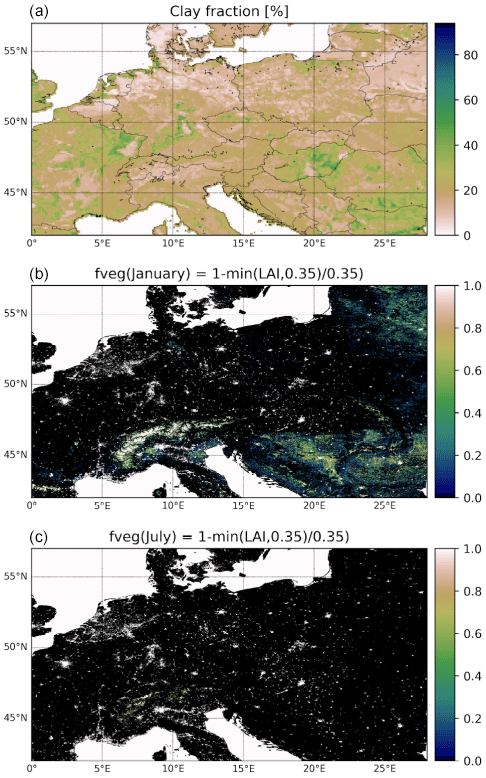
Figure 1 The input data for the clay fraction in percent (a) and the vegetation factor for January and July (b and c, respectively) based on MODIS 2010 LAI data.

The emission flux for dust in the size mode i in WBDUST is calculated by the following equation:

$$\begin{array}{}\text{(2)}& \begin{array}{rl}{j}_{\mathrm{emis},i}& ={\displaystyle \frac{c{\mathit{\rho }}_{\mathrm{air}}}{g}}(u_{*}+u_{*\mathrm{t}}{)}^{\mathrm{2}}(u_{*}-u_{*\mathrm{t}}){\mathrm{10}}^{-\mathrm{4}}\\ & \cdot \mathit{\alpha }{f}_{\mathrm{landcover}}{f}_{\mathrm{veg}}{M}_{i}N{S}_{\mathrm{topo}},\end{array}\end{array}$$

where c is an empirical constant (here = 1.5), u_* is the surface friction velocity, u_*t is the threshold surface friction velocity, f_landcover is the barren land fraction, f_veg is the vegetation factor, α is the sandblasting efficiency, ρ_air is the air density, g is the gravitational acceleration, M_i is the mass fraction emitted into the mode i, N is the normalization factor and, finally, S_topo is the topography factor parameter, which enhances the representation of emissions which are generated in valleys and basins. The equation for the threshold surface friction velocity can be found analytically in Klingmüller et al. (2018).

WBDUST is based on Fortran and is provided as a preprocessing tool along with the CAMx code (https://www.camx.com/download/support-software/; WBDUST, 2022). It is driven by WRF meteorological data (see below), while the required parameters are described in Sect. 2.4.

2.2 Driving meteorological model

To drive the dust model with meteorological data as well as to drive the chemical transport model used, the WRF (Weather Research and Forecasting) model version 4 (Skamarock et al., 2019) was used. In WRF, the radiation processes are parameterized by the RRTMG scheme (Iacono et al., 2008); microphysical processes and convection were treated by the Purdue Lin scheme (Chen and Sun, 2002) and the Grell-3D scheme (Grell, 1993), respectively. The description of surface layer processes followed the Eta model (Janjic, 1994). The land surface exchange is parameterized by the Noah (Chen and Dudhia, 2001), and, finally, the boundary-layer is resolved by the BouLac planetary boundary layer scheme (Bougeault and Lacarrère, 1989). Static land use data for WRF are derived from CORINE Land Cover data, version CLC 2012 (CORINE, 2012). For urban grid boxes, the single-layer urban canopy model (SLUCM; Kusaka et al., 2001) is used with the same urban parameters as in Karlický et al. (2018). The choice of physical parameterizations is based on results from Karlický et al. (2020), who performed a series of sensitivity experiments to achieve the best possible model–observation agreement. To drive the regional climate in WRF, the ERA-Interim reanalysis (Simmons et al., 2010) was used.

2.3 Chemical transport model

To account for the transport of the emitted dust and its interaction with the aerosol physical and chemical processes, we used the chemical transport model CAMx version 7.10 (Comprehensive Air-quality model with Extensions; Ramboll, 2020). CAMx is an Eulerian chemical transport model that simultaneously treats photochemistry and aerosol processes. As gas-phase chemistry and secondary aerosol formation are closely linked and, moreover, in our study we are interested in the impact of dust on secondary inorganic aerosol, we considered the “full” gas-phase chemistry in CAMx using the CB6r5 mechanism (Carbon Bond revision 6) described in Yarwood et al. (2010) and Emery et al. (2015).

For aerosol, a static two-mode (fine/coarse) approach called CF2E is adopted. Secondary inorganic aerosol is partitioned between gas and aerosol phases using either the ISORROPIA thermodynamic equilibrium model v1.7 (Nenes et al., 1998, 1999) or the EQSAM (EQuilibrium Simplified Aerosol Model V4) model (Metzger et al., 2016). ISORROPIA considers sulfate (PSO₄), nitrate (PNO₃), chloride (NCL), ammonium (PNH₄) and sodium (NA), with an update for calcium nitrate on dust particles, which is important for our study. Aqueous nitrate and sulfate formation in cloud water is computed using the RADM-AQ aqueous chemistry algorithm (Chang et al., 1987) with updated sulfur dioxide (SO₂) oxidation reaction rates and a metal-catalysed oxidation mechanism. A semi-volatile equilibrium scheme called SOAP (Strader et al., 1999) is used to form secondary organic aerosol from condensable vapours.

Apart from the secondary (in)organic aerosol, primary elemental (PEC) and primary organic carbon (POA), CAMx further considers general primary aerosol categories for fine crustal materials (dust; FCRS) and other fine primary aerosols (FPRM) and also for their coarse counterparts (CCRS and CPRM). The two-mode CF2E approach optionally includes eight explicit fine-mode elemental species: iron (Fe), manganese (Mn), calcium (Ca), magnesium (Mg), potassium (K), aluminium (Al), silicon (Si) and titan (Ti) which can be either modelled or background values of which are used for chemical calculations. Calcium is an exception and is scaled from FCRS and FPRM.

The species FPRM, FCRS, CPRM and CCRS including the eight elements do not chemically decay. However, light scattering by them and other PM components affecting photochemistry is considered. Furthermore, the fine-mode species concentrations influence PM and heterogeneous gas chemistry. In RADM-AQ, the oxidation of SO₂ to sulfate is catalytically enhanced by Fe and Mn, while Mg, Ca and K affect cloud pH, hence the solubility of SO₂. Further Mg, Ca and K influence inorganic aerosol partitioning in EQSAM, and Ca reacts with HNO₃ soil dust particles to form calcium nitrate (CaNO₃) in ISORROPIA. Fine aerosol species FPRM and FCRS along with the eight elements represent surface areas for heterogeneous reactions of SO₂ and N₂O₅. The uptake of SO₂ and HNO₃ by dust particles is also considered using a humidity-dependent uptake coefficient (Zheng et al., 2015).

CAMx was driven using WRF output translated to CAMx meteorological inputs using the wrfcamx preprocessor that is supplied along with the CAMx code https://www.camx.com/download/support-software/. The coefficients of vertical eddy diffusion (Kv) are diagnosed in wrfcamx based on the similarity method adopted from the CMAQ model (Byun and Ching, 1999). The choice of the method for the calculation of Kv is crucial as it greatly determines the species vertical transport, especially over urban environments (Huszar et al., 2020). They further showed that the CMAQ method represents the mid-range of the Kv intensities diagnosed from WRF output.

2.4 Experiments and data

A series of model simulations using CAMx coupled offline to WRF were carried out over a “larger” central European domain of the size of 189×165 grid cells (from France to Ukraine and northern Italy to Denmark) at a 9 km × 9 km horizontal resolution centred over Prague (Czechia) (50.075^∘ N, 14.44^∘ E; Lambert conic conformal projection). WRF has 40 layers in the vertical reaching 50 hPa, with the lowermost layer about 30 m thick. CAMx uses 18 layers, with the top one at about 10 km. As the long-term impact of WBD emissions is analysed here, we covered a 10-year simulation period from 1 January 2007 to 31 December 2016.

As already said, WRF was driven with the ERA-Interim reanalysis, while for CAMx chemical initial and boundary conditions we choose the CAM-Chem global model data (Buchholz et al., 2019; Emmons et al., 2020).

As anthropogenic emissions, the TNO-MACC-III data (an update of the MACC-II version; Kuenen et al., 2014) were used from 2011 for the whole period. This high-resolution ($\mathrm{1}/\mathrm{8}$^∘ longitude, $\mathrm{1}/\mathrm{16}$^∘ latitude; roughly 6 km × 6 km) European emission database provides annual emission estimates for NO_x, SO₂, non-methane volatile organic compounds (NMVOCs), methane (CH₄), ammonia (NH₃), carbon monoxide (CO), and PM₁₀ and PM_2.5 in 11 activity sectors. The annual emission totals were redistributed to model grid cells using the FUME (Flexible Universal Processor for Modeling Emissions) emission model (Benešová et al., 2018, http://fume-ep.org/, last access: 1 September 2022). FUME also took care of chemical speciation and time disaggregation of input, sector-based emissions, while the speciation and time disaggregation factors are based on Passant (2002) and van der Gon et al. (2011). The output of the FUME are CAMx-ready hourly emission data for the speciated model species. Biogenic emissions for CAMx are calculated offline with MEGANv2.1 (Model of Emissions of Gases and Aerosols from Nature) (Guenther et al., 2012) based on WRF meteorology and vegetation characteristics following Sindelarova et al. (2014).

For the WBDUST module, the inputs were the following. The land cover was described using the high-resolution (100 m) CORINE CLC 2012 land cover data (https://land.copernicus.eu/pan-european/corine-land-cover; CORINE, 2012) in combination with the United States Geological Survey (USGS) database for grid cells with no information from CORINE. This land use was used also for the CAMx dry-deposition scheme. The clay fraction data come from the Global Soil Dataset for use in Earth System Models (GSDE; Shangguan et al., 2014). The GSDE provides the clay fraction of the topmost 4.5 cm of the soil layer, which is most relevant for the sandblasting efficiency. Leaf area index data are taken from MODIS post-processed data provided by Yuan et al. (2011) at 30 s resolution (around 500 m over our domain) with an 8 d update interval. Year 2010 LAI was used for the whole period. As topography information to calculate the topography factor, the Global Multi-resolution Terrain Elevation Data 2010 (GMTED, 2010) were used, with a spatial resolution of 0.1^∘.

One of the important goals of the study is to examine the potential impact of WBD elemental composition (Na⁺, K⁺, Fe⁺, Mn⁺, Ca${}^{++}$ and Mg${}^{++}$) on the formation of secondary inorganic aerosol. Therefore, we must also consider the chemical soil composition of the emitted dust. We estimated it based on fractions that were calculated by Karydis et al. (2011).

The emissions of wind-blown dust (with the model described above) were calculated for fine and coarse crustal material based on WRF output meteorology: surface temperature, soil moisture, snow water equivalent, wind, temperature, pressure and geopotential height of the two lowermost levels. WBD emissions were thus calculated on an hourly basis (in accordance with output frequency). The calculation was done for six elements (Ca, Fe, Mg, Mn, K and Na), while the mass fraction of fine dust that does not belong to any of the listed elements is emitted as general fine crustal material (FCRS). Coarse crustal material is also emitted as one general species (CCRS).

In order to account for the sensitivity of the method for gas partitioning into the aerosol phase as well as due to the fact that the CAMx crustal elements interact with aerosol chemistry differently, we conducted CAMx experiments for both ISORROPIA and EQSAM. With each of these, a pair of experiments was conducted: (i) one without considering WBD (including anthropogenic aerosol emissions as well as anthropogenic and biogenic gas-phase emissions) and (ii) one with WBD considered. The experiments are accordingly named ISORROPIA_noWBD, ISORROPIA_WBD, EQSAM_noWBD and EQSAM_WBD.

In our analysis, we will examine the impact of WBD on PM_2.5 and PM₁₀ concentrations evaluated based on the ISORROPIA experiment pair. The EQSAM pair of simulations will be used to analyse the sensitivity of the impact of secondary aerosol chemistry. It is clear that if dust particles influence the heterogeneous aerosol chemistry, the total contribution of WBD will not simply be the sum of concentrations of FCRS and the listed elements, but instead, we have to account for the effect dust has on secondary aerosol. Therefore the impact will be calculated as follows:

$$\begin{array}{}\text{(3)}& \mathrm{\Delta }{\mathrm{PM}}_{\mathrm{2.5}}={\mathrm{PM}}_{{\mathrm{2.5}}_{\mathrm{WBD}}}-{\mathrm{PM}}_{{\mathrm{2.5}}_{\mathrm{noWBD}}},\end{array}$$

while ${\mathrm{PM}}_{{\mathrm{2.5}}_{\mathrm{WBD}}}$ is calculated as

$$\begin{array}{}\text{(4)}& \begin{array}{rl}{\mathrm{PM}}_{{\mathrm{2.5}}_{\mathrm{WBD}}}& =\mathrm{PEC}+\mathrm{POA}+\mathrm{FPRM}+{\mathrm{PSO}}_{\mathrm{4}}+{\mathrm{PNO}}_{\mathrm{3}}\\ & +{\mathrm{PNH}}_{\mathrm{4}}+\mathrm{SOA}+\mathrm{FCRS}+\mathrm{Ca}+\mathrm{Fe}+\mathrm{Mg}\\ & +\mathrm{Mn}+\mathrm{K}+\mathrm{Na}.\end{array}\end{array}$$

${\mathrm{PM}}_{{\mathrm{2.5}}_{\mathrm{noWBD}}}$ is calculated as

$$\begin{array}{}\text{(5)}& \begin{array}{rl}{\mathrm{PM}}_{{\mathrm{2.5}}_{\mathrm{noWBD}}}& =\mathrm{PEC}+\mathrm{POA}+\mathrm{FPRM}+{\mathrm{PSO}}_{\mathrm{4}}+{\mathrm{PNO}}_{\mathrm{3}}\\ & +{\mathrm{PNH}}_{\mathrm{4}}+\mathrm{SOA}+\mathrm{FCRS},\end{array}\end{array}$$

while FCRS here stands for fine crustal material entering the domain trough boundaries (it is not directly emitted in anthropogenic sources). For the impact on PM₁₀, we added CPRM and CCRS to these sums to account for the anthropogenic and dust coarse-mode aerosol, i.e.

$$\begin{array}{}\text{(6)}& \begin{array}{rl}\mathrm{\Delta }{\mathrm{PM}}_{\mathrm{10}}& =({\mathrm{CCRS}}_{\mathrm{WBD}}+{\mathrm{PM}}_{{\mathrm{2.5}}_{\mathrm{WBD}}})\\ & -({\mathrm{CCRS}}_{\mathrm{noWBD}}+{\mathrm{PM}}_{{\mathrm{2.5}}_{\mathrm{noWBD}}}).\end{array}\end{array}$$

Regarding CCRS_noWBD, as CCRS is not emitted in the noWBD simulations, this accounts for the crustal material entering the domain via the boundaries similar to the situation with FCRS above.

3 Results

3.1 Modelled WBD emissions

In this section, the dust emission fluxes calculated using the WBDUST emission module are analysed. The validation of the underlying meteorological conditions driving the emission model as well as the resulting PM concentrations are validated in the next section.

In Fig. 2, the two maps represent the seasonal average emissions for winter, the season with the highest emissions calculated. Winter-averaged FCRS dust emissions have values that can reach up to 0.5 $\mathrm{g}{\mathrm{s}}^{-\mathrm{1}}{\mathrm{km}}^{-\mathrm{2}}$, while CCRS dust emissions can reach values that exceed 1 $\mathrm{g}{\mathrm{s}}^{-\mathrm{1}}{\mathrm{km}}^{-\mathrm{2}}$. Increased emissions are noticed above western Germany, where much farmland and many agricultural areas are located. High emissions are also often concentrated around urban areas. Although the urban land use category is not regarded as bare soil, at the resolution used many of the urban grid boxes are only partly covered by urban land cover (only very few grid cells have an urban land cover of more than 50 %), and the rest is usually cropland which is potentially capable of dust emissions. As in the LAI input used (MODIS), it is often the cities which have sufficiently low LAI values (less than 0.35), it is there and over surrounding areas where the conditions for WBDUST emissions are met (low LAI and bare soil).

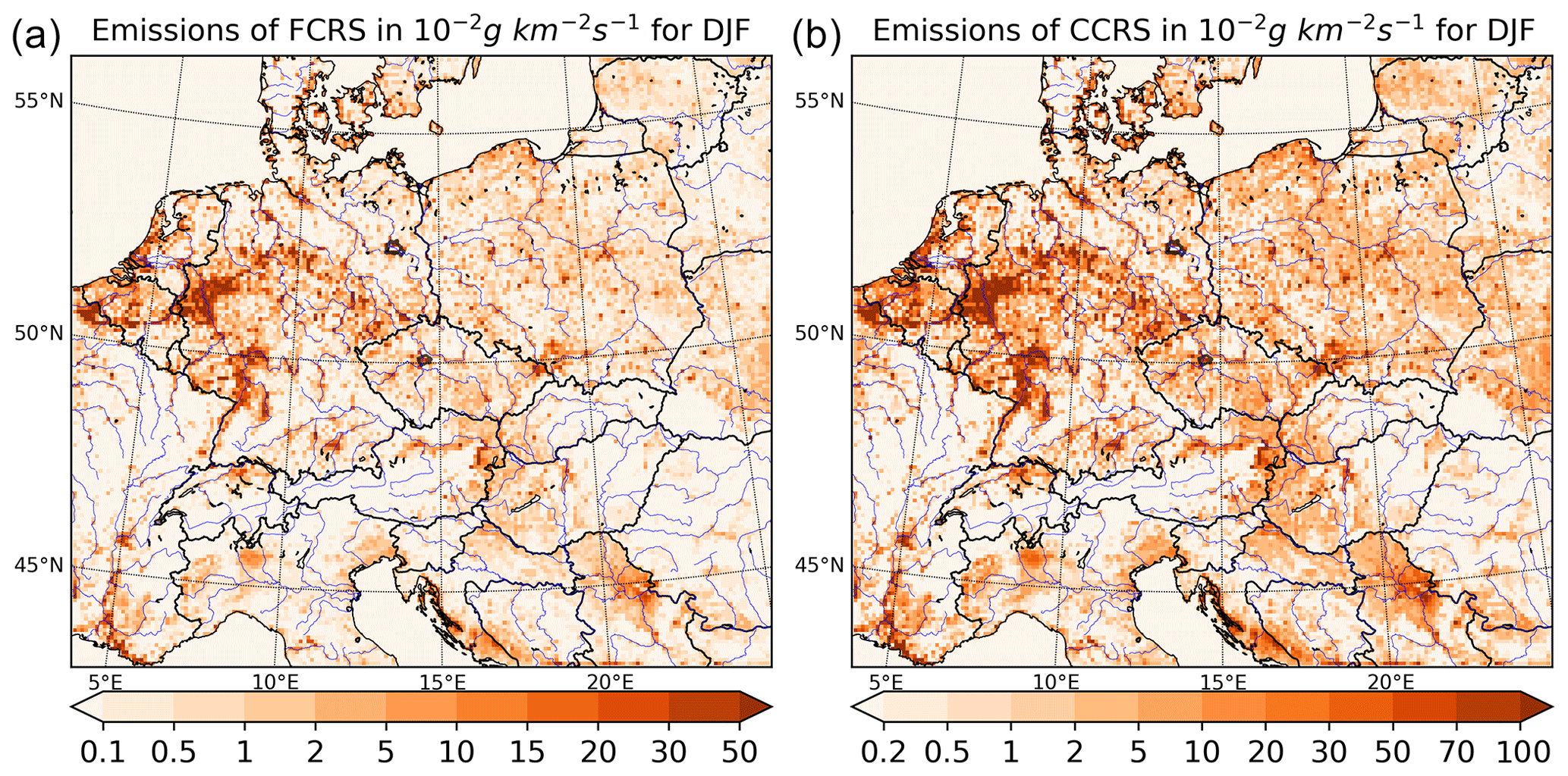
Figure 2 Average WBD emission fluxes of fine crustal material (FCRS; a) and of coarse crustal material (CCRS; b) above central Europe in DJF for the 2007–2016 period (in ${\mathrm{10}}^{-\mathrm{2}}\mathrm{g}{\mathrm{s}}^{-\mathrm{1}}{\mathrm{km}}^{-\mathrm{2}}$). Note that the colour bars differ.

The seasonal variability was also assessed by calculating the average annual cycle of the monthly mean domain-averaged emissions. Figure 3 confirms that higher emissions occur in the winter season for both FCRS and CCRS, while the main emitting period begins in October and ends in April, proving that the presence of winds along with low LAI is the governing factor for dust emissions.

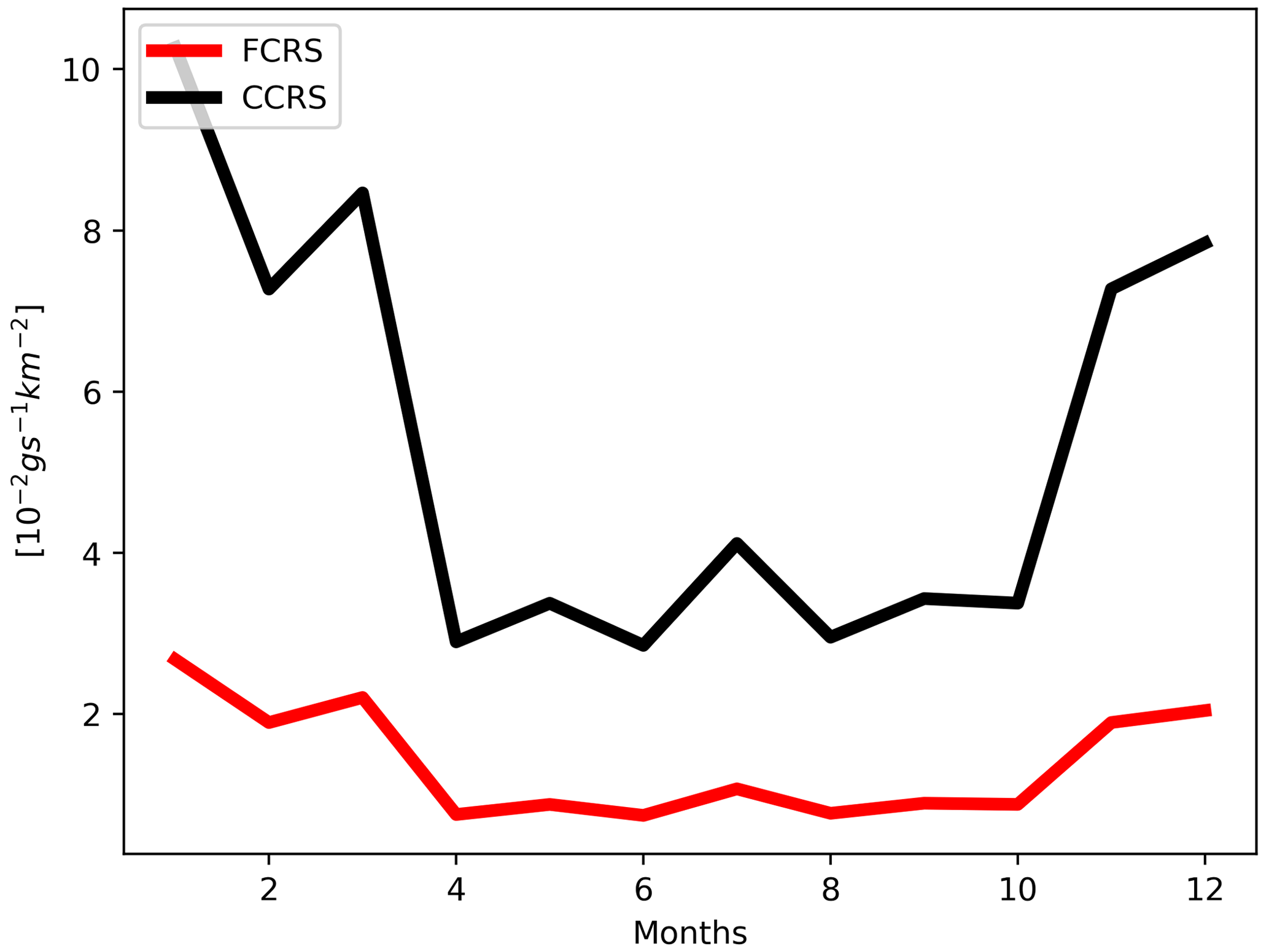
Figure 3 Domain-averaged annual cycle of monthly averages of FCRS and CCRS WBD emission fluxes for 2007–2016 (in ${\mathrm{10}}^{-\mathrm{2}}\mathrm{g}{\mathrm{s}}^{-\mathrm{1}}{\mathrm{km}}^{-\mathrm{2}}$).

The temporal variability of these emissions on a daily and hourly basis is shown in terms of the daily average values and the average diurnal cycle, respectively. Figure 4 represents the time series of the domain-averaged daily averages. A high variability of daily emissions is seen and FCRS emissions can exceed 0.5 $\mathrm{g}{\mathrm{s}}^{-\mathrm{1}}{\mathrm{km}}^{-\mathrm{2}}$, while CCRS emissions can reach values higher than 1 $\mathrm{g}{\mathrm{s}}^{-\mathrm{1}}{\mathrm{km}}^{-\mathrm{2}}$ on specific days.

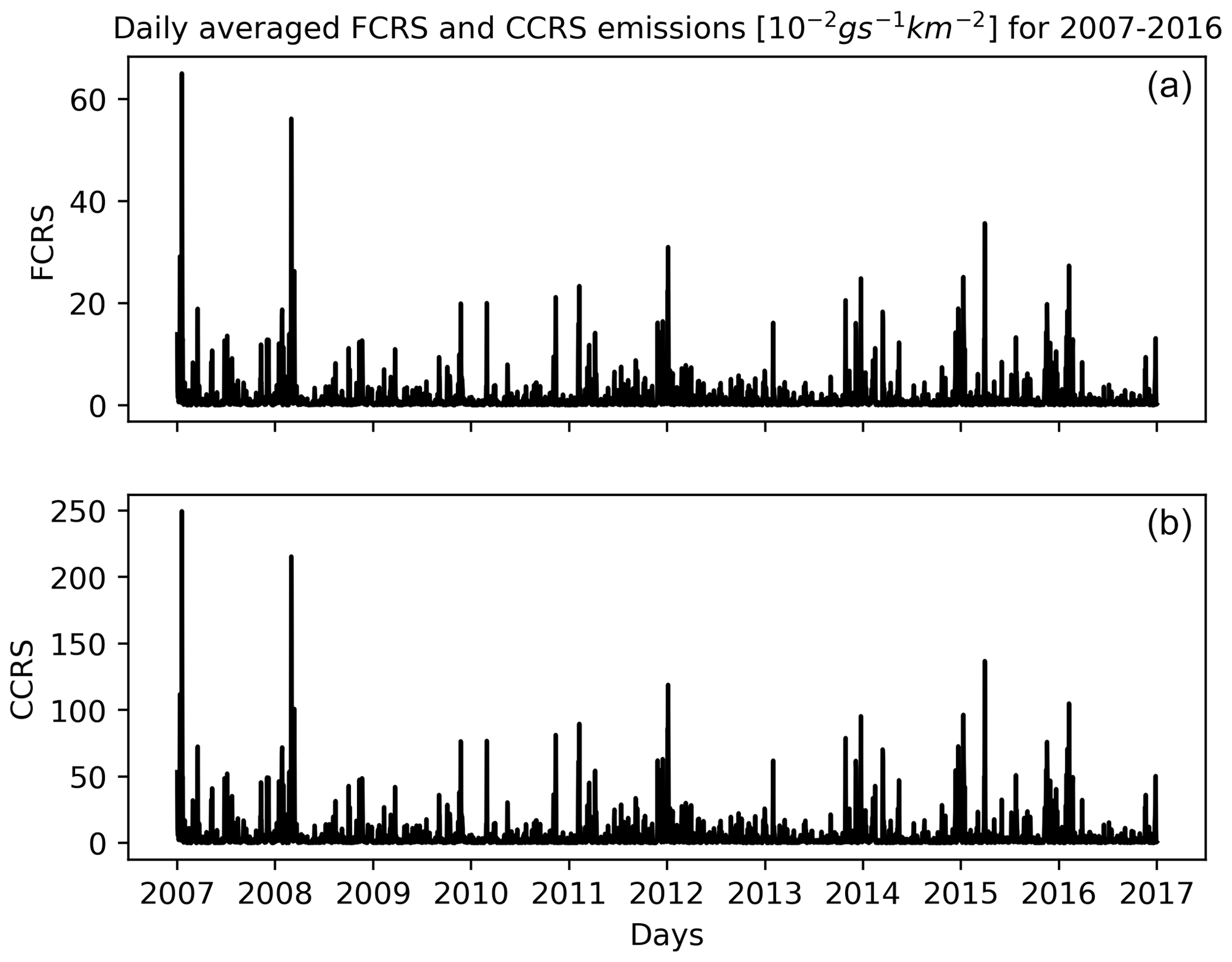
Figure 4 Domain-averaged daily WBD emission fluxes of FCRS (a) and CCRS (b) for 2007–2016 (in ${\mathrm{10}}^{-\mathrm{2}}\mathrm{g}{\mathrm{s}}^{-\mathrm{1}}{\mathrm{km}}^{-\mathrm{2}}$).

Figure 5 shows the average diurnal cycle of the average hourly emission fluxes for different seasons. Emissions peak at midday, which is associated with stronger winds and usually lower stability enabling the sandblasted soil to be lifted to produce emissions. The daily amplitudes are about 0.5–1 × 10⁻² and 2–4 × 10⁻² g s⁻¹ km⁻² for FCRS and CCRS, respectively.

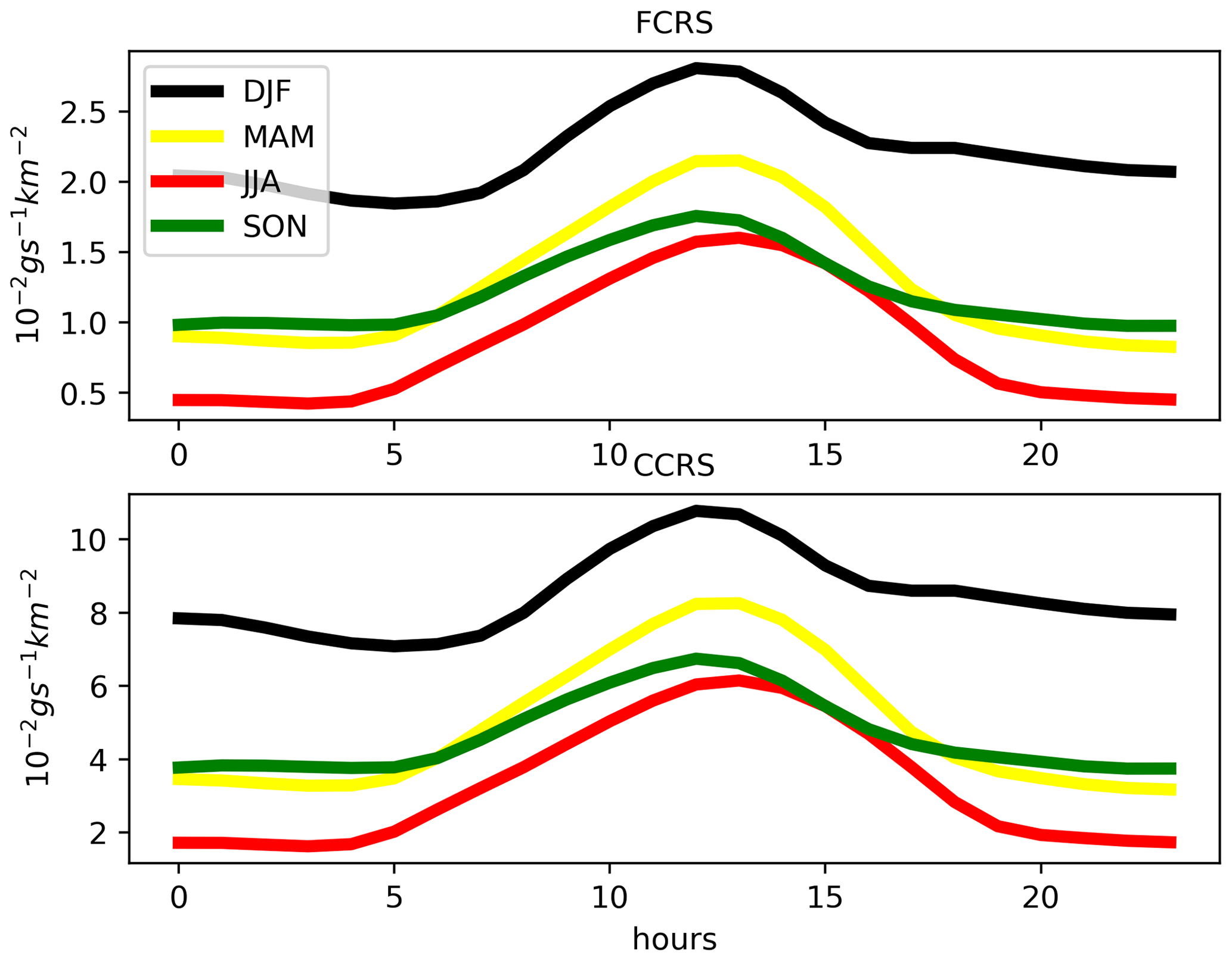
Figure 5 Domain-averaged diurnal cycle of hourly FCRS and CCRS WBD emission fluxes for different seasons for 2007–2016 (units are ${\mathrm{10}}^{-\mathrm{2}}\mathrm{g}{\mathrm{s}}^{-\mathrm{1}}{\mathrm{km}}^{-\mathrm{2}}$).

Sensitivity to wind speeds and LAI

Knowing the strong dependence of WBD emission fluxes on wind speed values, we conducted two additional calculations. We reduced wind speeds entering the WBDUST model by a factor of 0.75 and 0.5 (motivated by the observed positive wind bias; see Sect. 3.2.1).

Further, we also tested the sensitivity to LAI (via the derived vegetation factor; see Sect. 2.1) averaging from MODIS over grid cells with an urban land cover fraction, which, as already mentioned above, causes some locally increased WBD emissions near urban areas. In our setup, about 400 MODIS LAI data points fall into one CAMx grid cell, and we averaged LAI data only for the non-urban fraction of a grid cell by excluding the fraction of the lowest MODIS LAI values (usually zero) from averaging that correspond to the urban fraction. In other words, we assumed that the higher LAI values within these 400 points are associated with the non-urban grid cell fraction.

The results of these sensitivity tests are presented in Fig. 6, where the spatial distribution of winter WBD emissions is presented for the default case as well as for the 0.75 and 0.5 reduction in wind speeds and finally for the modified LAI averaging. For the 0.75 reduction, emissions are reduced and reach up to 10–15 × 10⁻² g s⁻¹ km⁻², with peaks of up to 20 × 10⁻² g s⁻¹ km⁻². This means that through a 25 % reduction in wind speeds, emissions are reduced by a factor of 2 to 3. With a much stronger reduction of 50 % of the original wind speeds, the resulting WBD emissions are reduced much more strikingly, i.e. by 2 orders of magnitude, and reach 30–50 × 10⁻⁴ g s⁻¹ km⁻². This means that on many of the modelled days, the wind speed values probably fell below the threshold friction velocity (u_*) resulting in zero emissions and implying very low DJF average emissions. Finally, for the modified LAI averaging, we see that emissions do indeed decrease near cities (by about 50 %), partly removing the artificial emission peaks.

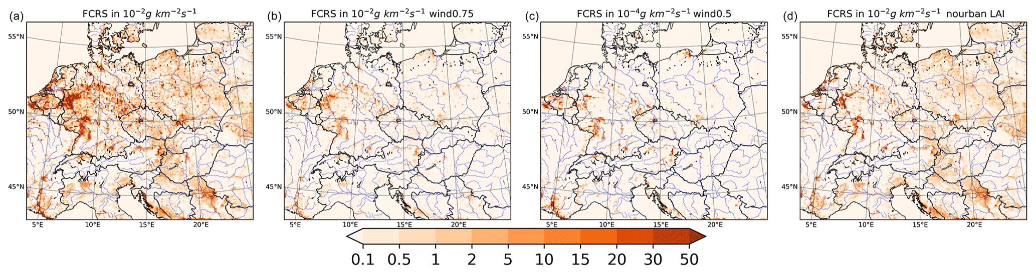
Figure 6 Average WBD emission fluxes of fine crustal material (FCRS) above central Europe in DJF for 2007–2016. From (a) to (d): the default WBD emissions, WBD emissions after a 0.75× reduction in wind speeds, WBD emissions after a 0.5× reduction in wind speeds and emissions with LAI averaged only over non-urban grid cell fractions. Note that the units for the 0.5 wind reduction have an order of 10⁻⁴, while the rest have an order of 10⁻².

3.2 Validation

3.2.1 Meteorological fields

As the modelled WBDUST emissions depend on meteorological conditions and the state of the soil, it is important to evaluate how well the driving model (WRF) represents the meteorological conditions that affect emission fluxes the most. In this section we compare the modelled temperature and wind speed with available measurements from the area of Czechia, while the soil moisture will be compared with satellite data. Although Czechia represents a small fraction of the entire domain, we expect that the model biases are representative of larger areas. Measured temperature and wind data are from 10 automated pollution monitoring stations (“Automatizovaný́ imisní monitoring”, AIM; https://www.chmi.cz, last access: 20 March 2023) of the Czech Hydrometeorological Institute (CHMI) which, besides air quality data, also provides meteorological measurements.

Starting with the temperature, Fig. 7 represents the seasonal 2007–2016 averaged diurnal cycles. It is clear that the daily maximum temperatures are underestimated by the model during summer (JJA), while a better match is achieved in other seasons. The autumn (SON) data show some positive model bias too. Regarding daily minima, the model tends to overestimate them for summer and autumn, while a clear underestimate occurs in winter (DJF). The above-mentioned biases are always less than 2 ^∘C and usually less than 1 ^∘C.

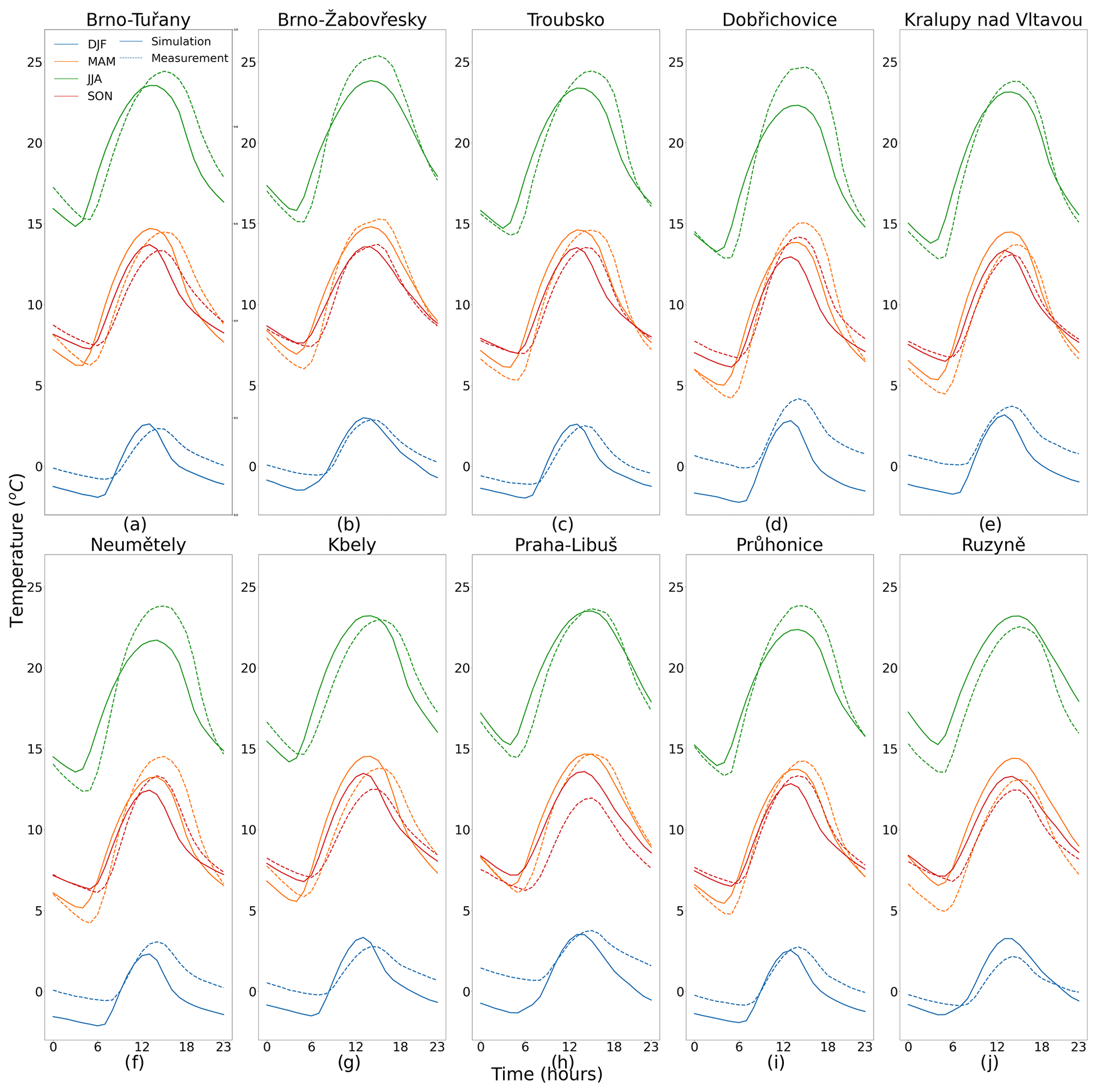
Figure 7 Comparison of modelled temperature diurnal profiles (solid) with measurements (dashed) from 10 Czech stations averaged over different seasons for the 2007–2016 period. Units in ^∘C.

As, from a dust emission perspective, the maximum wind speeds are more relevant than the average ones, we also compared the modelled monthly mean of the maximum daily wind speeds averaged over 2007–2016. Results are depicted in Fig. 8. It is clear that the model captures the annual cycle of wind reasonably well, with minima during the late summer and early autumn and maximum wind speeds during winter. However, a strong positive model bias is evident, reaching 2–4 m s⁻¹, except at the Praha-Ruzyně station and in Brno-Tuřany during summer.

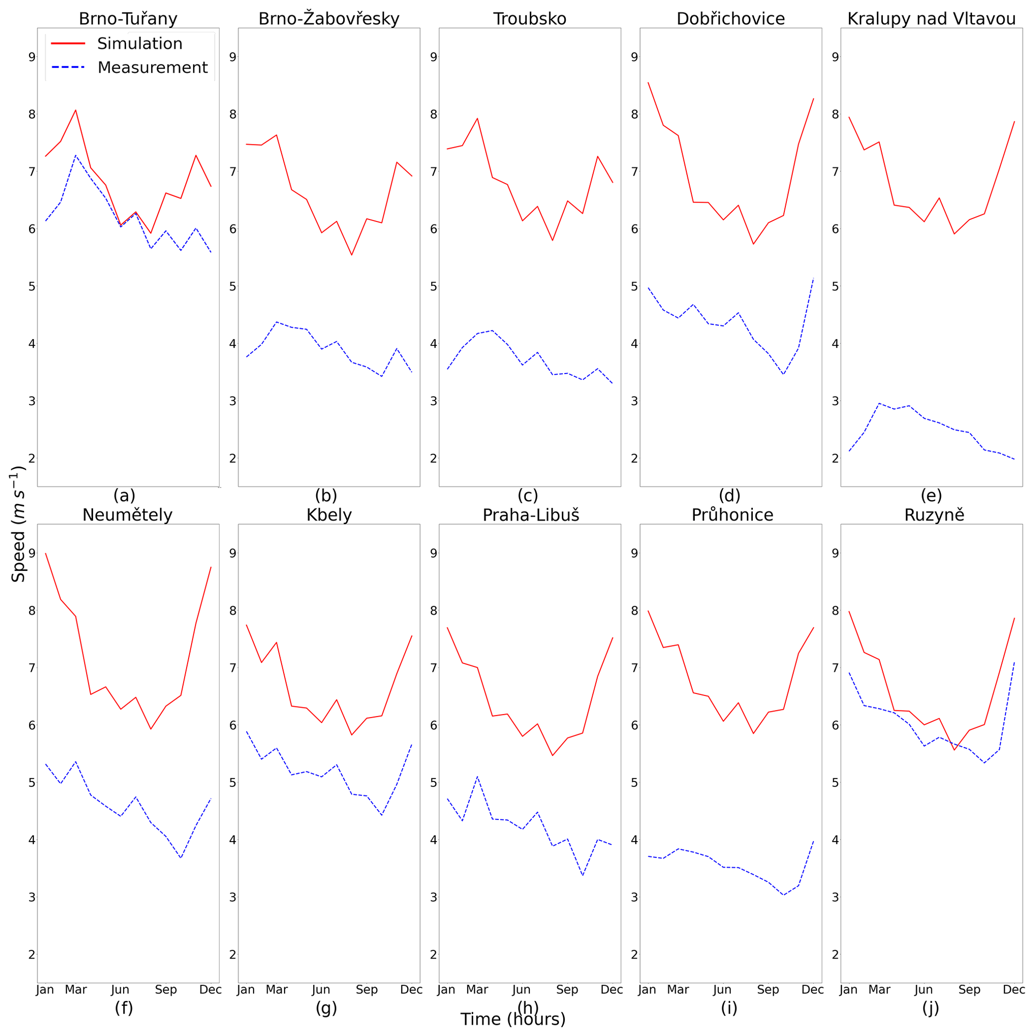
Figure 8 Comparison of the modelled annual cycle of the monthly mean of maximum daily wind speeds (solid red lines) with measurements (dashed blue lines) from 10 Czech stations averaged over the 2007–2016 period. Units are metres per second.

Finally, the state of the soil in terms of moisture content is another key driver of emissions with low soil moisture promoting sandblasting and thus dust emissions. For this quantity, we used the ESA CCI SM v07.1 satellite-based dataset (Dorigo et al., 2017; Gruber et al., 2019) and plotted the spatial distribution (for the area of Czechia) of the 2007–2016 seasonal-mean volumetric soil moisture in Fig. 9. The satellite data show strong annual variation, with minimum values during summer (0–0.2 m³ m⁻³), while the values are much higher during winter (0.4–0.6 m³ m⁻³). This annual cycle is seen also in the modelled data but is much weaker, with summer soil moisture data slightly lower than the winter ones. It is also clear that the model overestimates the observed data, especially during summer, while the winter overestimation is small (with model values around 0.4–0.5 m³ m⁻³), with some underestimation even limited to small regions.

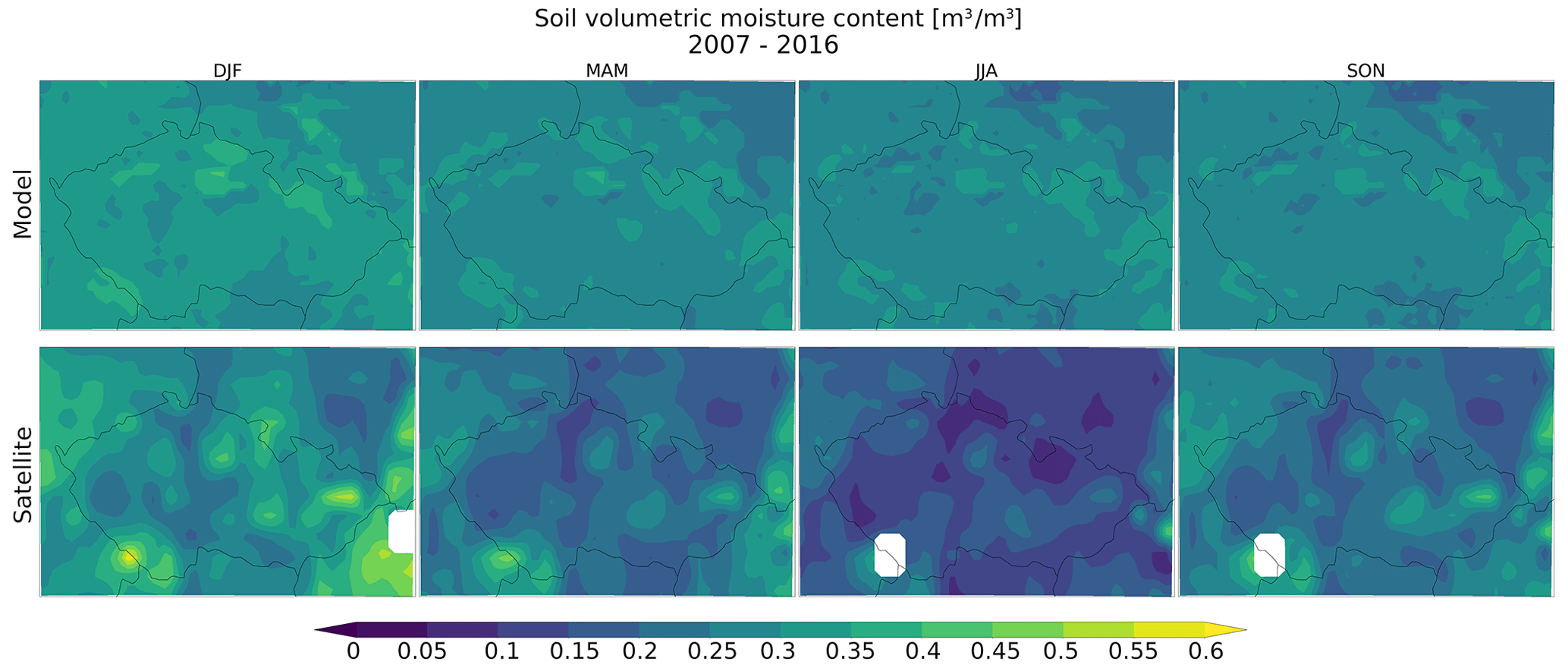
Figure 9 Comparison of modelled seasonal volumetric soil moisture (upper row) with the ESA CCI soil moisture data (lower row) for the area of Czechia. Data averaged over 2007–2016. Units are cubic metres per cubic metre.

3.2.2 PM concentrations

In this section, our results will be validated by comparing the modelled PM_2.5 and PM₁₀ concentrations calculated by CAMx (by the ISORROPIA experiment pair) with observations. The observations were retrieved from AirBase, the European air quality database (https://discomap.eea.europa.eu/map/fme/AirQualityExport.htm; EEA, 2021), with available “(sub)urban-background” stations from selected European cities (i.e. Vienna, Prague, Berlin, Munich, Budapest and Warsaw). These observations were plotted along with WBD and noWBD CAMx concentrations, averaged daily for the six European cities for 2007–2016.

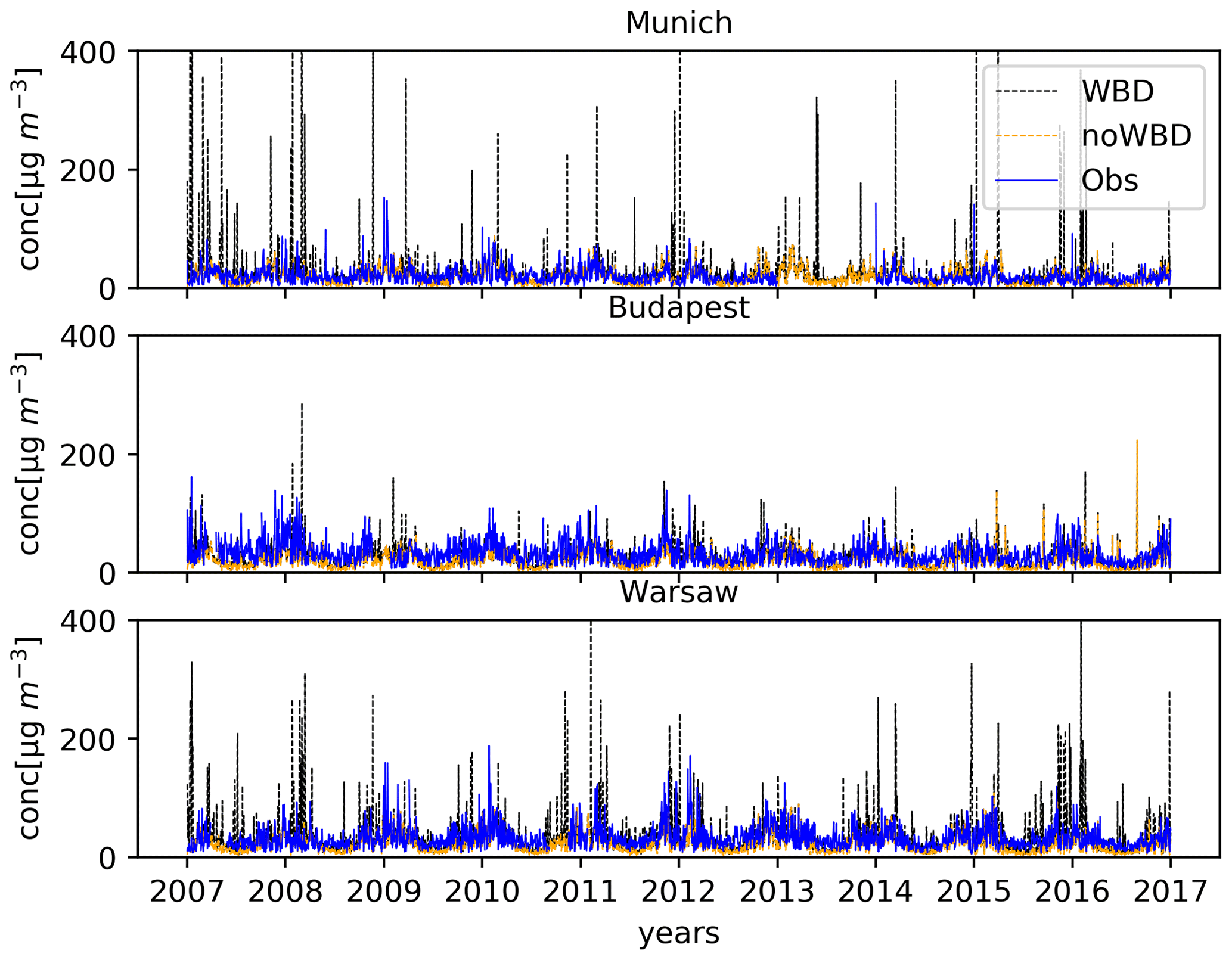
Figures 10 and 11 depict daily time series for modelled and measured PM_2.5 concentrations for selected European cities. In general, the time evolution of observed values is captured well by the model simulations. It is also seen that during the summer months, concentrations are usually underestimated. For winter, when the highest measured peaks occur (often exceeding 100 µg m⁻³), the model often fails to correctly capture the strength of the peak or its timing. It is also clear (and expected) that the WBD simulation generates the highest peaks, which are closer to the observed peaks, or even exceeds the observed ones, suggesting a positive model bias during winter. For PM₁₀ (Figs. 12 and 13) the situation is similar in underestimating summer values, while those for winter are also often overestimated in the WBD simulation when very strong peaks occur (up to several 100 µg m⁻³; e.g. for Prague, Munich or Warsaw, reaching almost 500 µg m⁻³) which are not seen in the noWBD simulation. This probably suggests a strong overestimation of the wind-blown dust emissions generating these peaks.

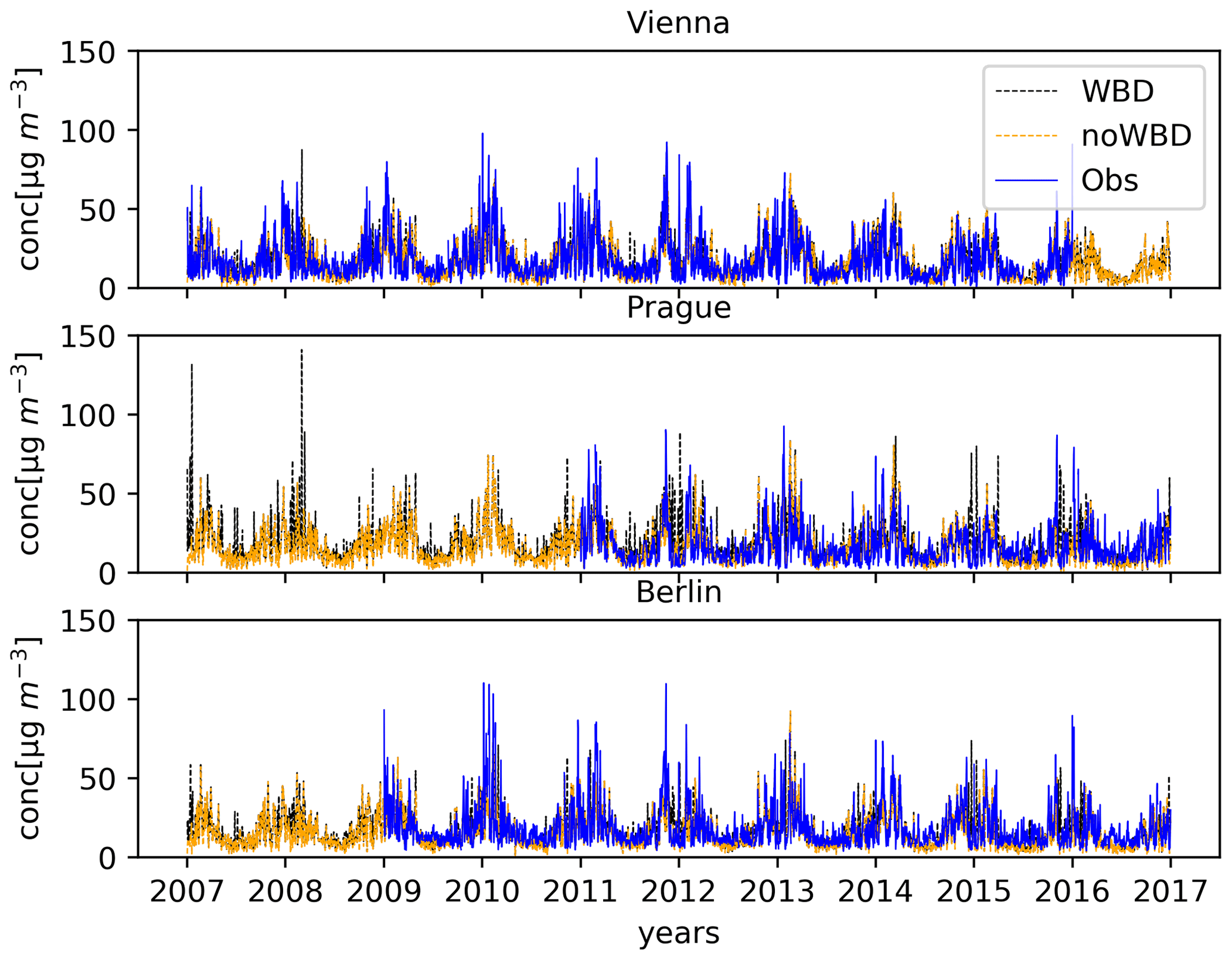
Figure 10 Averaged daily PM_2.5 concentrations of WBD (dashed black lines), noWBD (dashed orange lines) and the AirBase dataset (solid blue lines) for 2007–2016 (Vienna, Prague, Berlin). Units are micrograms per cubic metre.

Figure 11 Same as Fig. 12 but for Munich, Budapest and Warsaw.

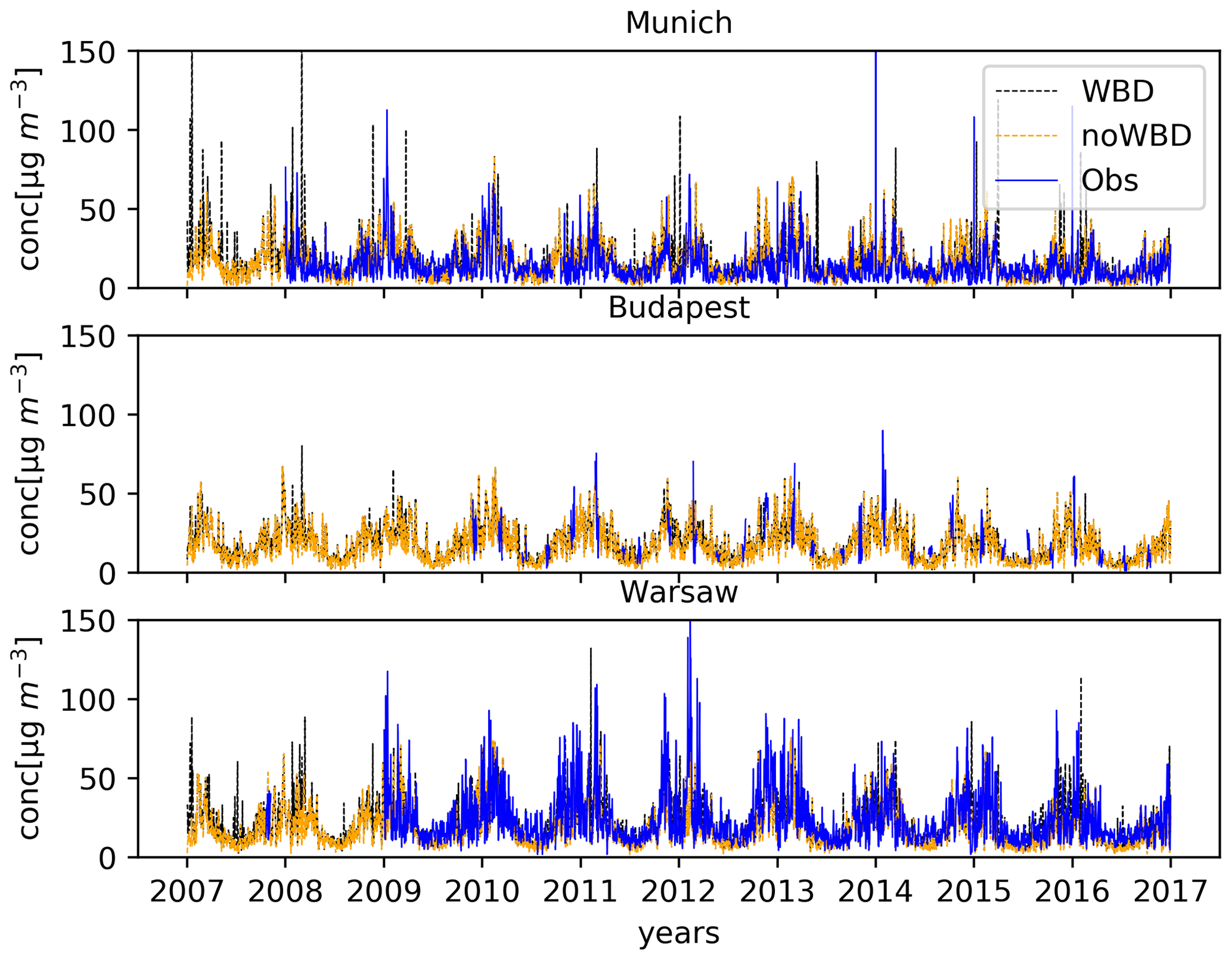
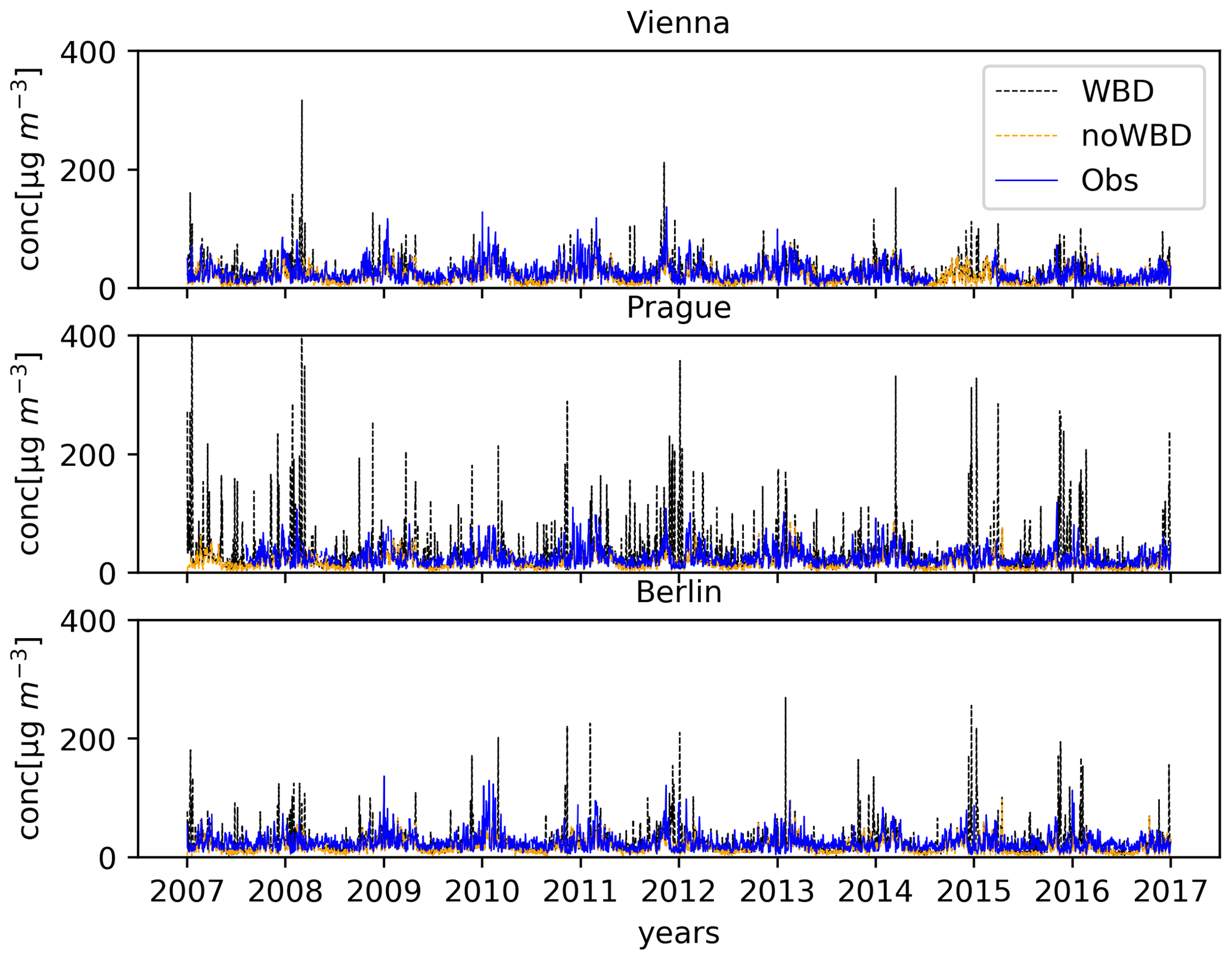
Figure 12 Averaged daily PM₁₀ concentrations of WBD (dashed black lines), noWBD (dashed orange lines) and the AirBase dataset (solid blue lines) for 2007–2016 (Vienna, Prague, Berlin). Units are micrograms per cubic metre.

Figure 13 Same as Fig. 12 but for Munich, Budapest and Warsaw.

In Figs. 14 and 15 the annual cycles of monthly mean concentrations for PM_2.5 and PM₁₀ are shown. All PM_2.5 concentrations fluctuate with the same trend, having their highest values during the winter and autumn seasons. The magnitude of the difference between the modelled data for WBD and noWBD and the observations is around 5–10 µg m⁻³. Summer months are underestimated, while the inclusion of wind-blown dust reduces this negative bias. In winter the modelled values are overestimated in Munich and Prague, while they are underestimated in Berlin, Budapest and Warsaw. Depending on this, the inclusion of dust emissions increases (e.g. Prague, Munich) or decreases (Vienna, Warsaw, Budapest) the model bias. In the case of PM₁₀, summer values are underestimated in noWBD simulation by about 10–20 µg m⁻³, while this underestimation is clearly reduced to 0–10 µg m⁻³ for the WBD simulations. A different situation occurs in winter, when the noWBD model values underestimate the measured data (by a similar magnitude as in summer); however, the inclusion of dust emissions increases model values such that a positive model bias is generated. This is in line with the daily time series seen above, when strong peaks occur in the WBD simulation, which are probably the main cause of these seasonal biases.

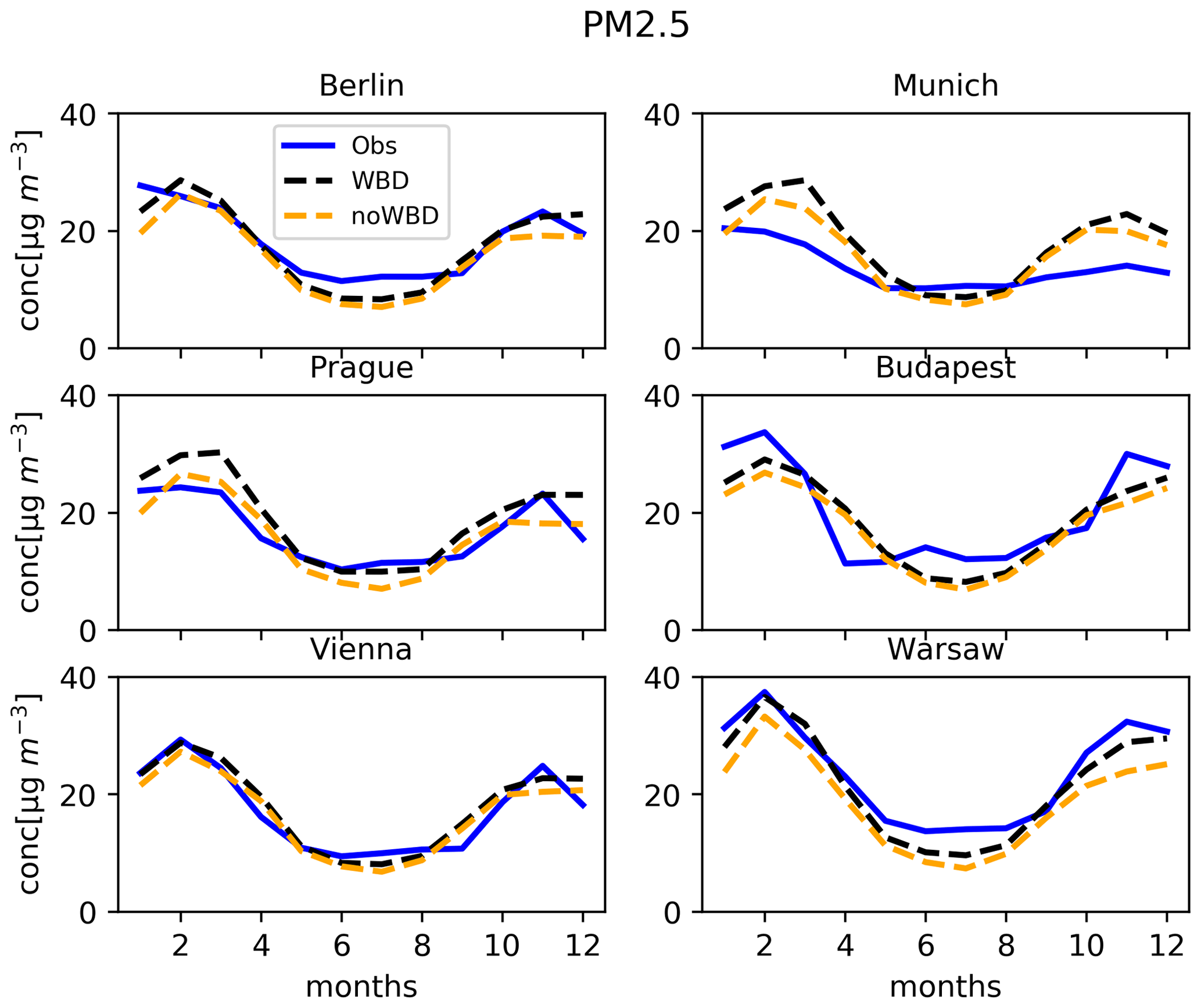
Figure 14 Annual cycle of monthly PM_2.5 concentrations of the WBD (dashed blue lines) and noWBD (dashed orange lines) simulations and the AirBase dataset (solid blue lines) for 2007–2016.

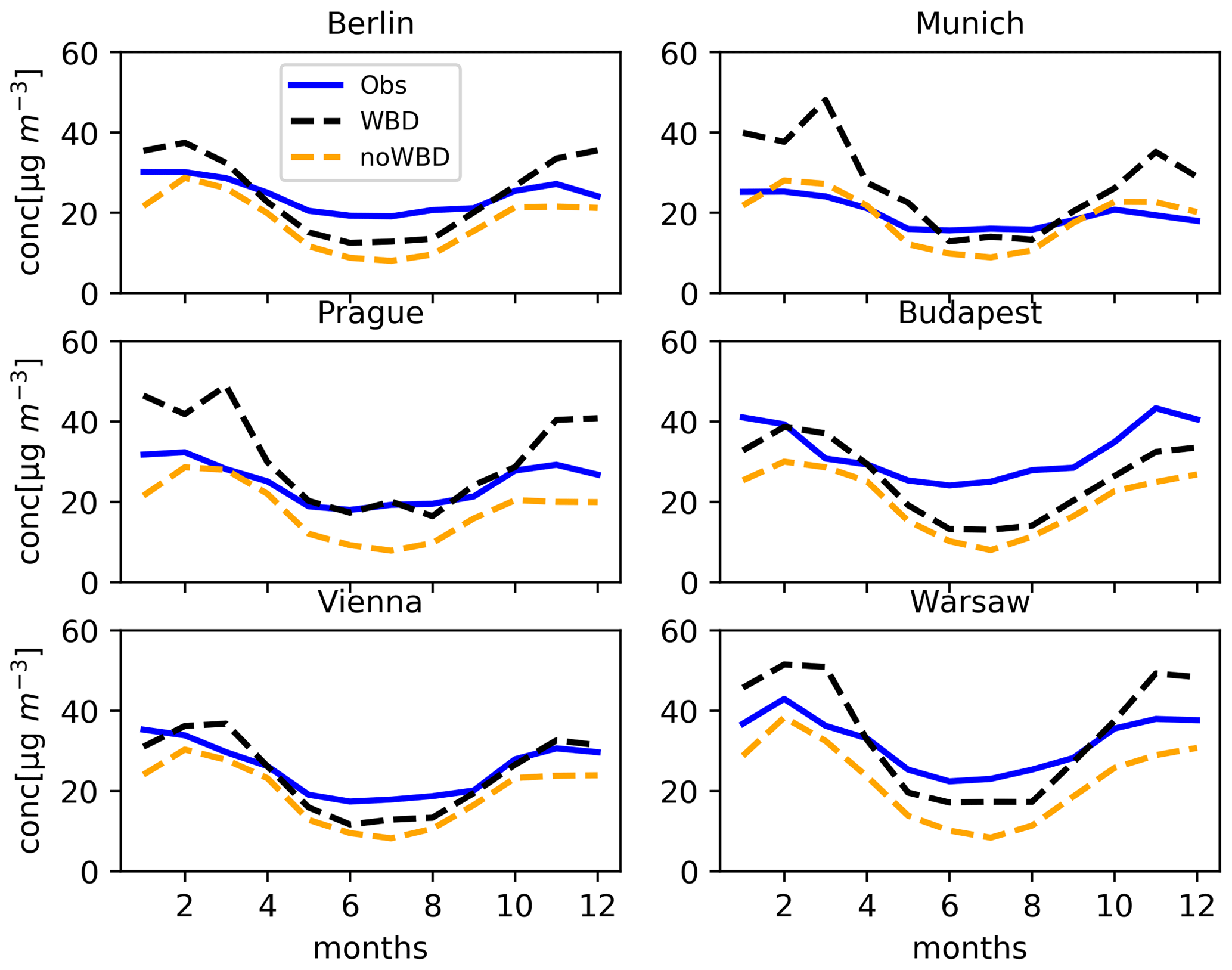
Figure 15 Annual cycle of monthly PM₁₀ concentrations of the WBD (dashed blue lines) and noWBD (dashed orange lines) simulations and the AirBase dataset (solid blue lines) for 2007–2016.

To gain more quantitative information on whether the inclusion of WBD emissions reduced/enhanced the model biases, we calculated several statistical measures presented below.

In Tables 1 and 2, the Pearson correlation coefficient, the root mean squared error (RMSE) and the normalized mean bias (NMB) were calculated for the daily mean concentrations of PM_2.5 and PM₁₀ in each city based on all values and on seasonal selection. We calculated the statistics separately for WBD and noWBD ISORROPIA simulations.

Table 1 Annual and seasonal statistical measures (Pearson correlation, RMSE, NMB) for PM_2.5 for both WBD and noWBD ISORROPIA simulations calculated from the daily averages.

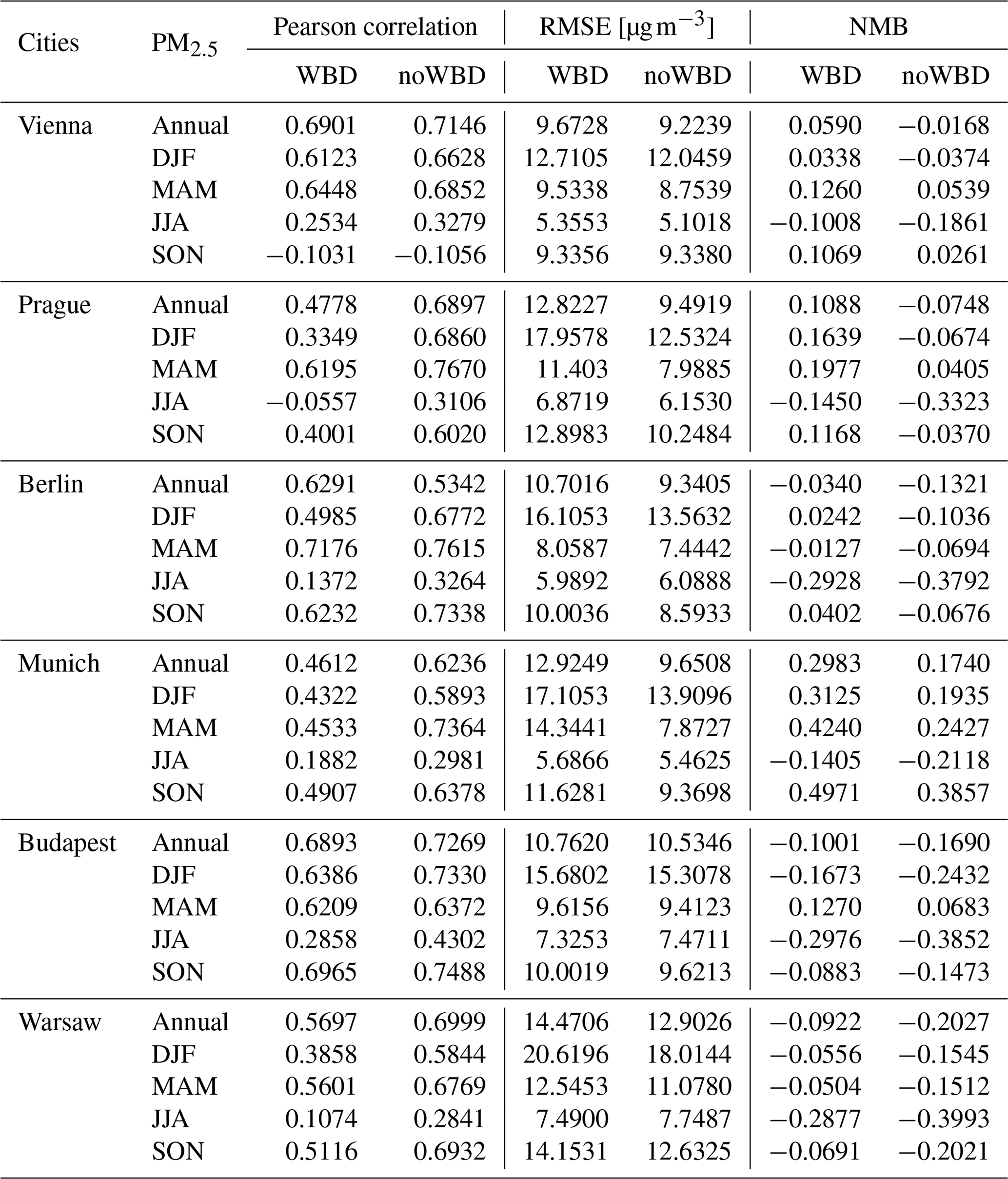
Table 2 Annual and seasonal statistical measures (Pearson correlation, RMSE, NMB) for PM₁₀ for both the WBD and noWBD ISORROPIA simulations calculated from the daily averages.

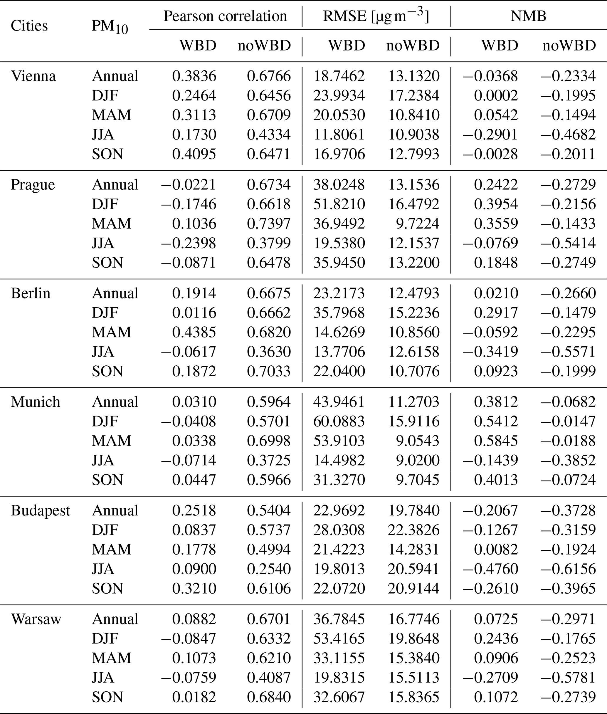
The Pearson correlation measures the strength of the linear relationship between the modelled data and the observed ones. RMSE is the standard deviation of the residuals (prediction errors). It indicates how concentrated the data are around the line of best fit, and, finally, the normalized mean bias (NMB) indicates the average deviation of the modelled values from the observed ones. These statistics are generated from all model–observation pairs from each station in a particular city.

The annual correlations of daily PM_2.5 and PM₁₀ with measurements are around 0.5–0.7 depending on the city, while the seasonal values are smallest for JJA (around 0.2–0.4) and highest in DJF and MAM. An important result is that the correlations are much smaller for the WBD simulations, which indicates that the wind-blown dust emissions are poorly correlated with the real dust emissions that occurred. This is seen also for the RMSE, which has values of between 5 and 20 µg m⁻³ for PM_2.5 and between 10–40 µg m⁻³ for PM₁₀, and evidently, the WBD values are higher. On a seasonal level, the lowest RMSEs are encountered for JJA. In the case of mean bias, annual values for PM_2.5 are up to −0.2 for the noWBD simulations. In this case, the WBD brought improvement for some cities, resulting in a lower absolute NMB. This is especially due to JJA values where NMB improved for all cities. For PM₁₀, annual NMBs are also negative and reach −0.37. In this case, the WBD annual NMBs are also lower for almost every city compared to the noWBD values. On seasonal levels, the improvement, i.e. lower mean biases, is also evident.

The result raises the question of whether strong winds in WRF are responsible for overestimated WBD emissions and consequently PM concentration. To test this hypothesis, we chose Prague and selected those days when the model bias is positive and larger then 50 µg m⁻³ (see Fig. 12). Then we used this mask and repeated the wind comparison from Sect. 3.2.1 but selecting only the stations in and around Prague and averaging only over such days. The results are depicted in Fig. 16 for four stations. From the figure, it is clear that wind speeds for such days are greater than the average for all days and reach values of about 10–12 m s⁻¹, which is about 50 % higher than the averages for all days seen in Fig. 8. The bias, however, remained similar; i.e. the modelled wind speeds are 50 %–100 % than the observed ones. This means that the relative bias of model winds retained its magnitude throughout all of the days in the examined period. However, in Fig. 6 we showed a very strong sensitivity of WBD emissions to wind speed, and a 50 % change can significantly change the emission magnitude and thus concentrations of PM.

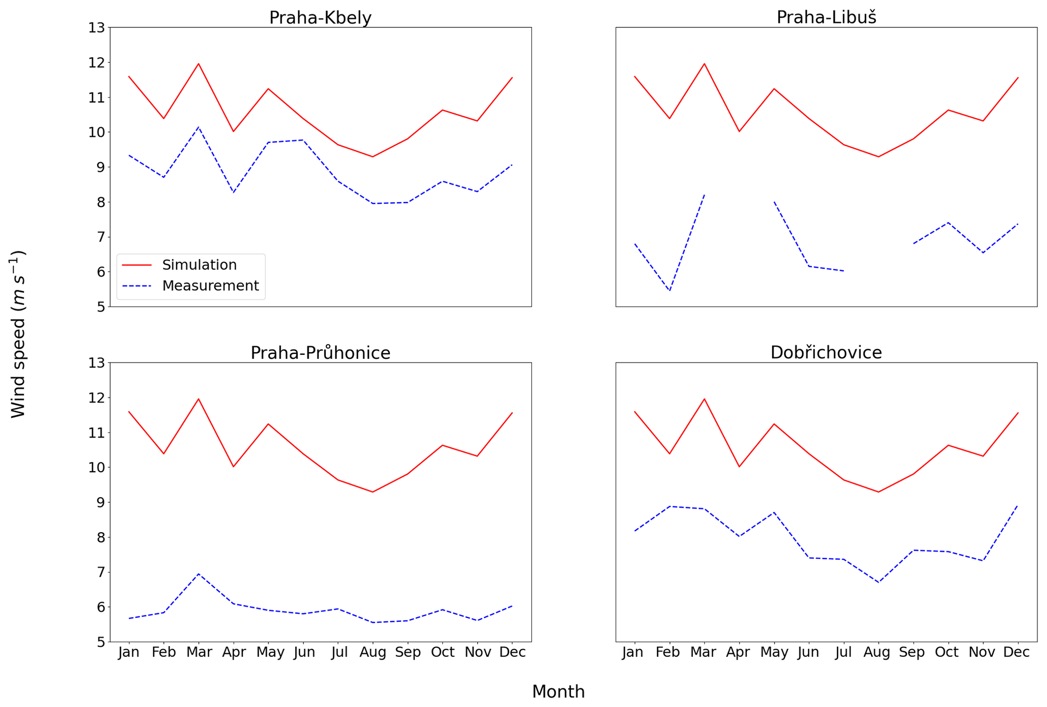
Figure 16 Annual cycle of monthly averaged maximum daily wind speeds from model simulations (red) and observations from four station in or around Prague (blue); averaging is done for days when the daily PM₁₀ model bias is larger than 50 µg m⁻³.

In summary, by including wind-blown dust emissions, the correlation of the daily PM_2.5 and PM₁₀ (hereafter represented as PM${}_{\mathrm{2.5}/\mathrm{10}}$) values decreased strongly and the RMSE increased. This can be explained by the many outliers in the modelled PM data. Both the correlation and the RMSE are very sensitive to such values. For NMB, improvement for PM₁₀ was achieved for almost all seasons and cities, while for PM_2.5, the improvement occurred only for the summer months. Overall it seems that model skill deteriorates when WBD emissions suddenly increase due to strongly overestimated winds.

3.3 Impact of WBD emissions on PM

In this section, the spatial distribution and the temporal evolution of the impact of dust emissions on PM_2.5 and PM₁₀ concentrations are presented (i.e. the ΔPM_2.5 and ΔPM₁₀ from Eqs. 3 and 6). Starting with the temporal evolution, Figs. 17 and 18 represent the WBD impact on PM_2.5 and PM₁₀ concentrations for selected cities in central Europe.

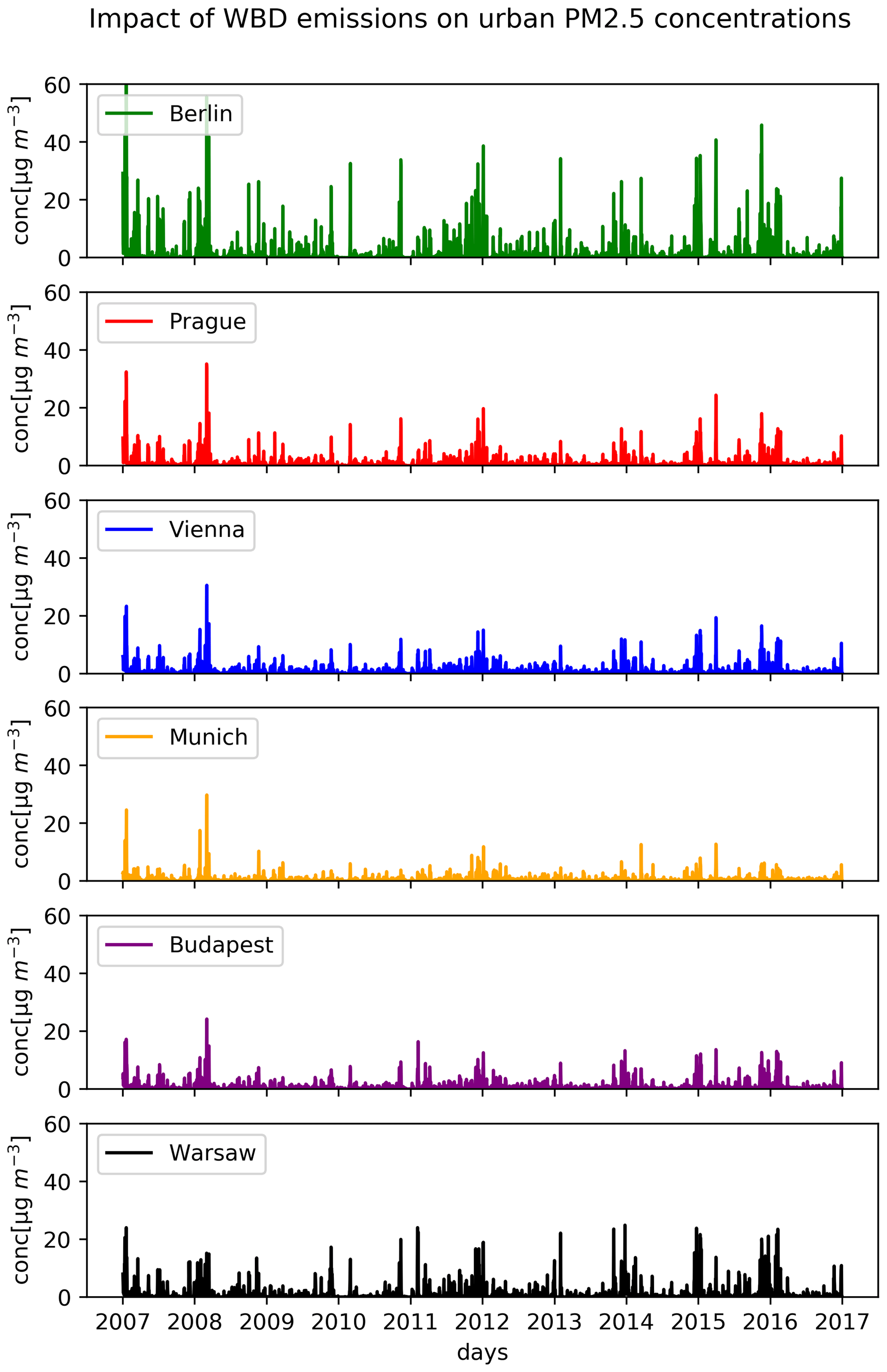
Figure 17 Daily averaged impact of wind-blown dust emissions on PM_2.5 concentrations in micrograms per cubic metre for 2007–2016.

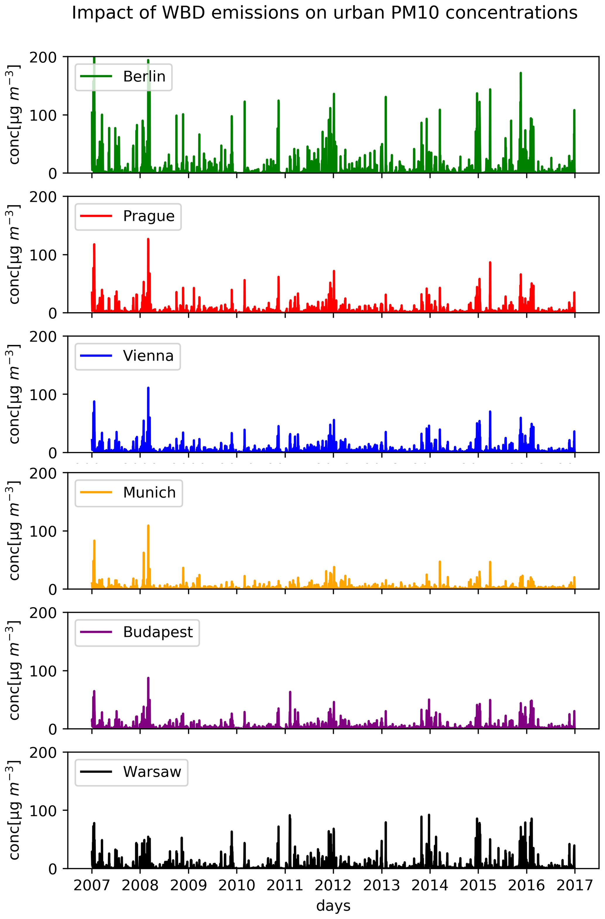
Figure 18 Daily averaged impact of wind-blown dust emissions on PM₁₀ concentrations in micrograms per cubic metre for 2007–2016.

The WBD impact on PM_2.5 daily urban concentrations can reach values of up to 30 µg m⁻³, where the highest values are noticed in Berlin, contributing up to 60 µg m⁻³ to the total PM_2.5 concentrations. The corresponding WBD impact on PM₁₀ concentrations is higher than expected and can reach values of more than 80 µg m⁻³, with Berlin again representing the highest extremes with values of up to 200 µg m⁻³. It is also clear that the highest impacts on PM are modelled in wintertime in accordance with the annual cycle of emissions seen earlier.

To obtain spatial information on the WBD impact on PM, Fig. 19 depicts the seasonally averaged (2007–2016) dust impact on PM_2.5 (left; ΔPM_2.5) and PM₁₀ (right; ΔPM₁₀) concentrations above central Europe. The dust contribution to PM_2.5 concentrations can reach values of up to 12 µg m⁻³ in DJF and about 8 µg m⁻³ in other seasons, while the highest impacts are modelled over Germany and over central Europe near large urban areas. In winter, a large part of the domain exhibits an impact above 1 µg m⁻³. The impact on PM₁₀ is characterized by higher values of up to 20 µg m⁻³, mainly in DJF, while the spatial distribution is very similar to the PM_2.5 impact, being highest above western Europe (mainly Germany) with values above 2 µg m⁻³ over other areas. The impacts seen are in line with the highest emissions calculated in Fig. 2.

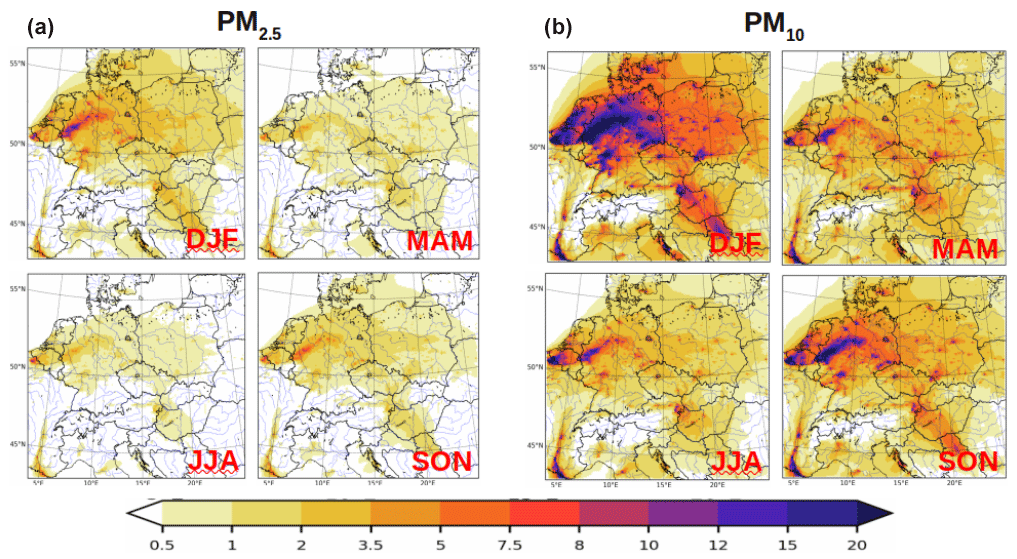
Figure 19 Seasonally averaged impact of WBD emissions on PM_2.5 (a) and PM₁₀ (b) concentrations in micrograms per cubic metre for 2007–2016.

To further support the hypothesis that the peak values in the daily concentrations are seen in PM₁₀ (Figs. 13 and 12) as well as in the impact figures (Fig. 18), we present the scatter plot of the daily mean concentrations of PM₁₀ values above Prague vs. the WBD emissions from around this city (average of 10 × 10 grid cells) in Fig. 20. The two colours distinguish concentration values below and above the 100 µg m⁻³ threshold. The figure shows that for values below this threshold, high concentrations are obtained even for very low WBD emissions, which is probably a result of anthropogenic emissions. However, for high concentrations (blue colour), it is clear that they correlate with the emissions of wind-blown dust.

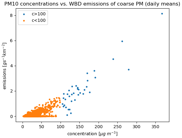
Figure 20 Scatter plot of the daily mean CAMx concentrations of PM₁₀ corresponding to Prague city centre vs. WBD emissions of coarse PM (CCRS) from the 90 km × 90 km area around Prague for the 2007–2016 period. Orange/blue circles stand for concentrations below/above 100 µg m⁻³.

Impact on PM components

As mentioned above, PM_2.5 concentrations contain secondary constituents, and in this section, we investigate how the presence of wind-blown dust (FCRS and elements Ca, Fe, Mg, Mn, K, Na) would affect the concentrations of the anthropogenic secondary inorganic aerosols. Figure 21 depicts the seasonally averaged WBD impact on PSO₄, PNO₃ and PNH₄ for the ISORROPIA experiment.

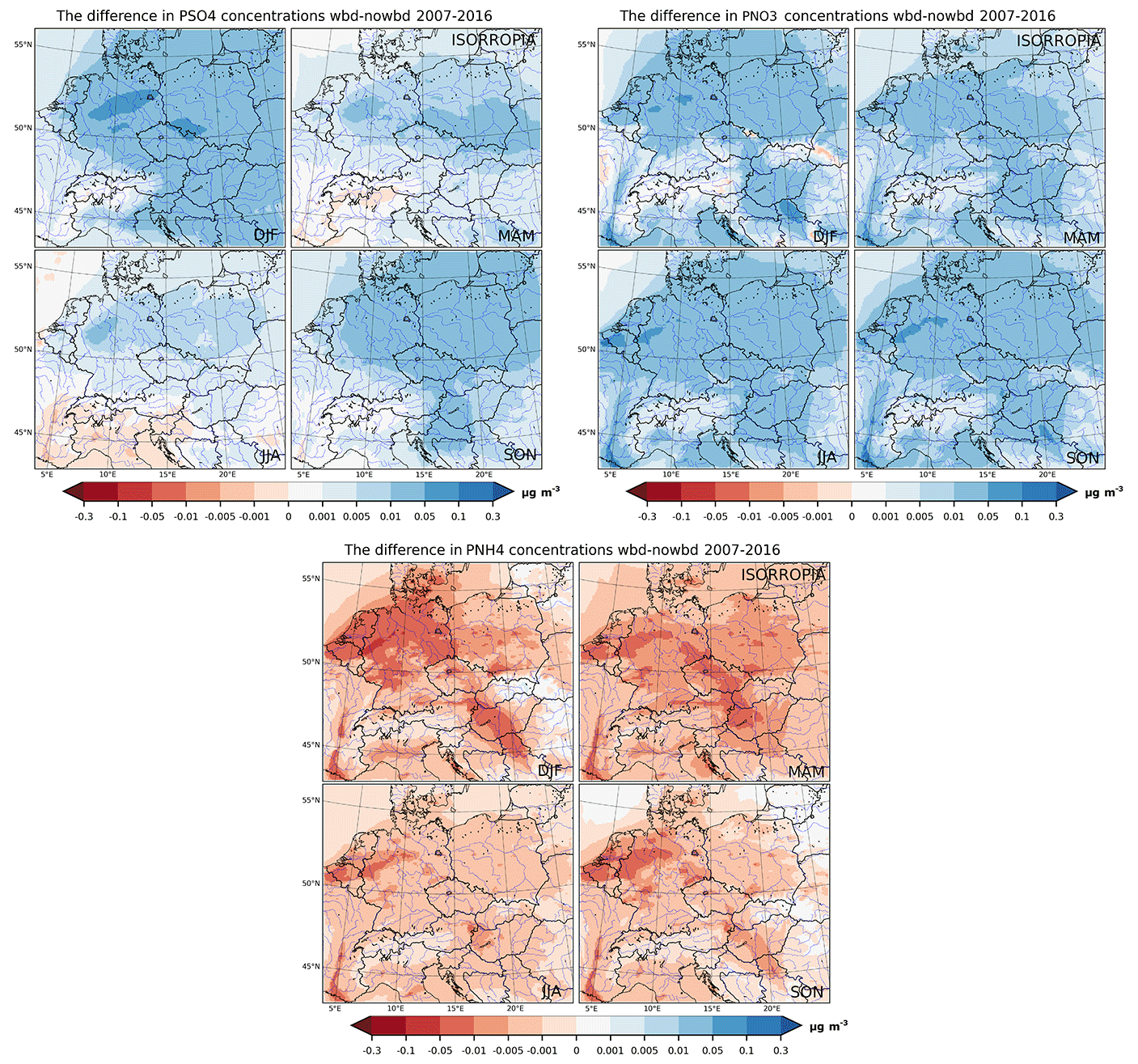
Figure 21 The WBD emission impact on secondary inorganic aerosol concentrations (PSO₄, PNO₃ and PNH₄) with ISORROPIA, seasonally averaged, in micrograms per cubic metre for 2007–2016.

Regarding sulfates, the strongest impacts occur during the winter reaching 0.1 µg m⁻³ over parts of Germany and Poland. In other seasons the impact remains less than 0.05 µg m⁻³, while it can be slightly negative in summer, reaching −0.01 µg m⁻³. PNO₃ is shown to be increased with the presence of WBD too, with values of up to 0.1 µg m⁻³ in all seasons, while most of the domain exhibits an increase of above 0.01 µg m⁻³. Finally, PNH₄ is decreased above the entire domain with values often exceeding −0.05 µg m⁻³ and peaks decreasing by around −0.1 µg m⁻³ especially over the western part of the domain in winter.

The impact of WBD on secondary inorganic aerosol in the EQSAM experiments (Fig. 22) is evidently stronger in magnitude. The impact on PSO₄ sometimes exceeds 0.1 µg m⁻³, and the negative impact over Italy is also stronger. In the case of nitrates the impact also sometimes exceeds 0.1 µg m⁻³, and a larger area is marked with an increase of above 0.05 µg m⁻³ compared to ISORROPIA. Finally, for ammonium, the decrease is larger than 0.01 µg m⁻³ and can exceed 0.1 µg m⁻³, being evidently stronger than in the ISORROPIA experiment.

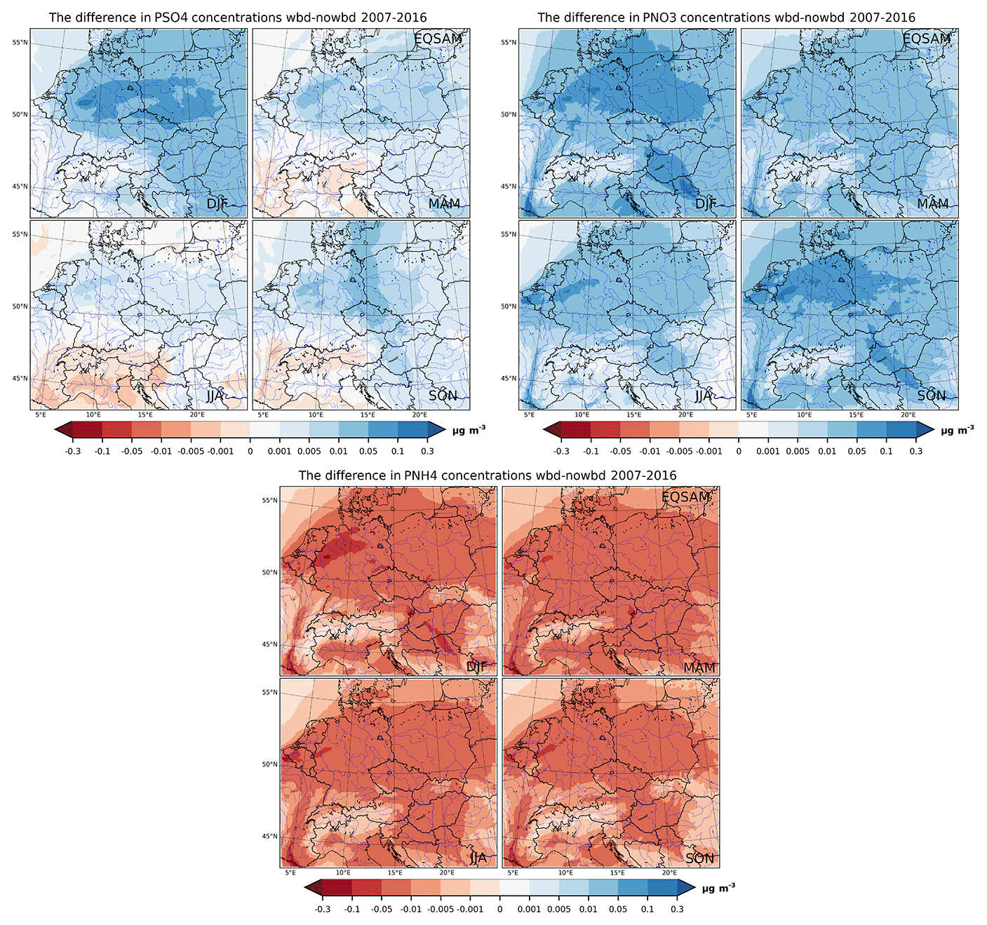
Figure 22 The WBD emission impact on secondary inorganic aerosol concentrations (PSO₄, PNO₃ and PNH₄) with EQSAM, seasonally averaged, in micrograms per cubic metre for 2007–2016.

The geographical distribution of the seasonally averaged impact does not provide information about the possible daily extremes of the impacts of WBD on secondary aerosol. Therefore we also plotted the temporal evolution of the averaged daily change in PSO₄, PNO₃ and PNH₄ concentrations due to WBD over the six selected urban areas.

Figure 23 shows the WBD impact on sulfates, while Figs. 24 and 25 show the impact on nitrates and ammonium, respectively.

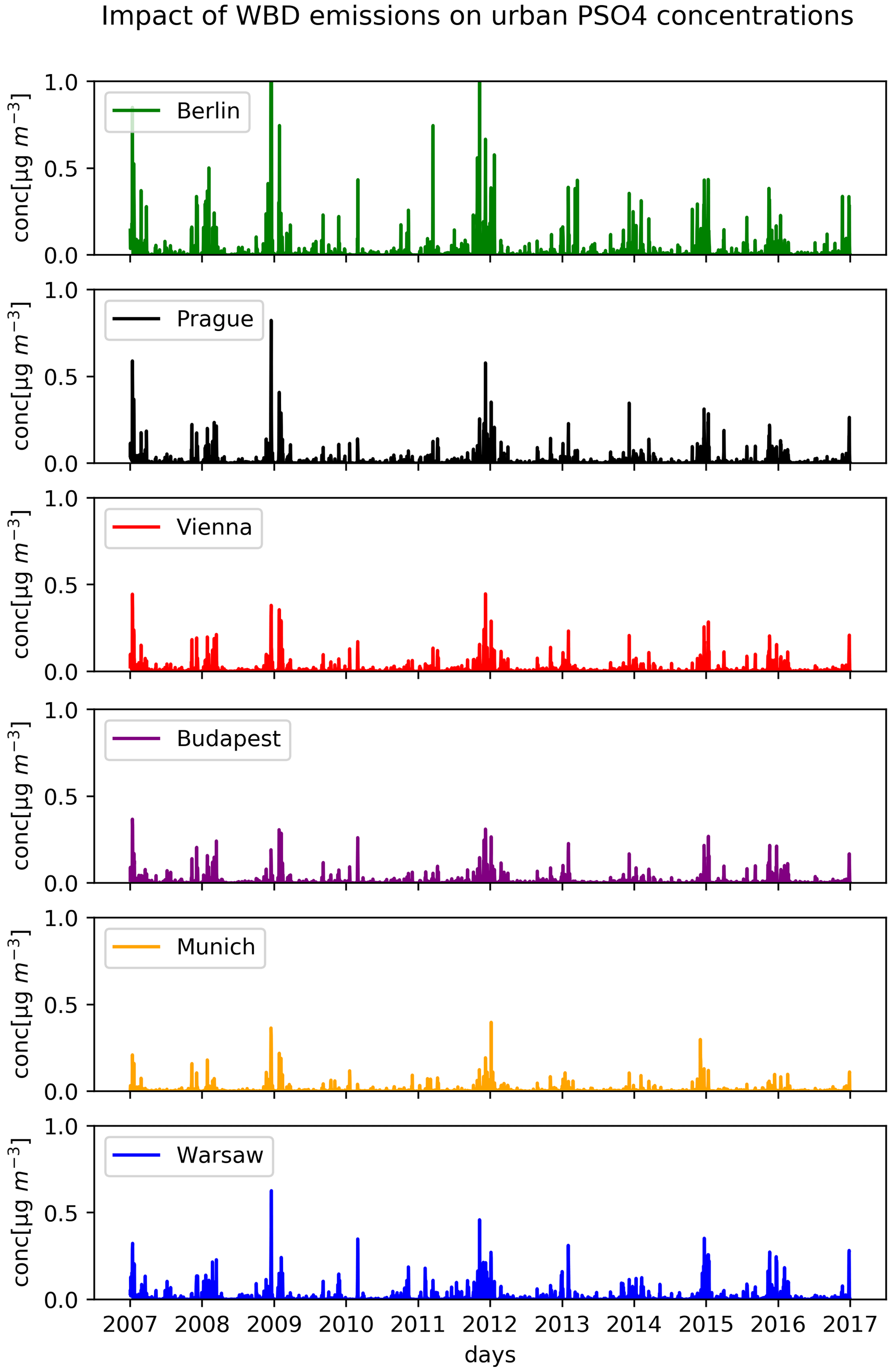
Figure 23 The long-term WBD impact on PSO₄ concentrations in ISORROPIA, averaged daily for 2007–2016. Units are micrograms per cubic metre.

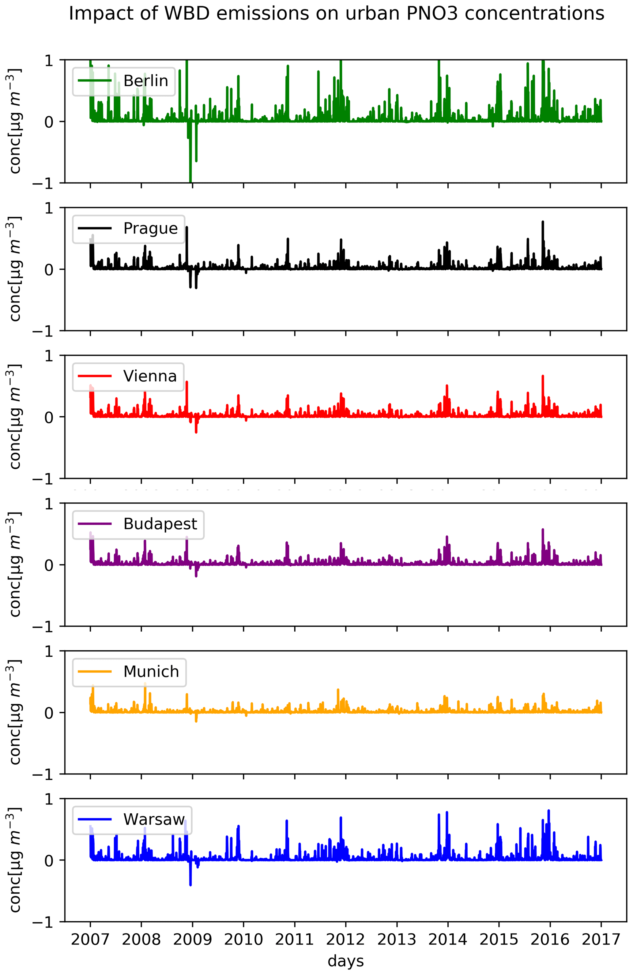
Figure 24 The long-term WBD impact on PNO₃ concentrations in ISORROPIA, averaged daily for 2007–2016. Units are micrograms per cubic metre.

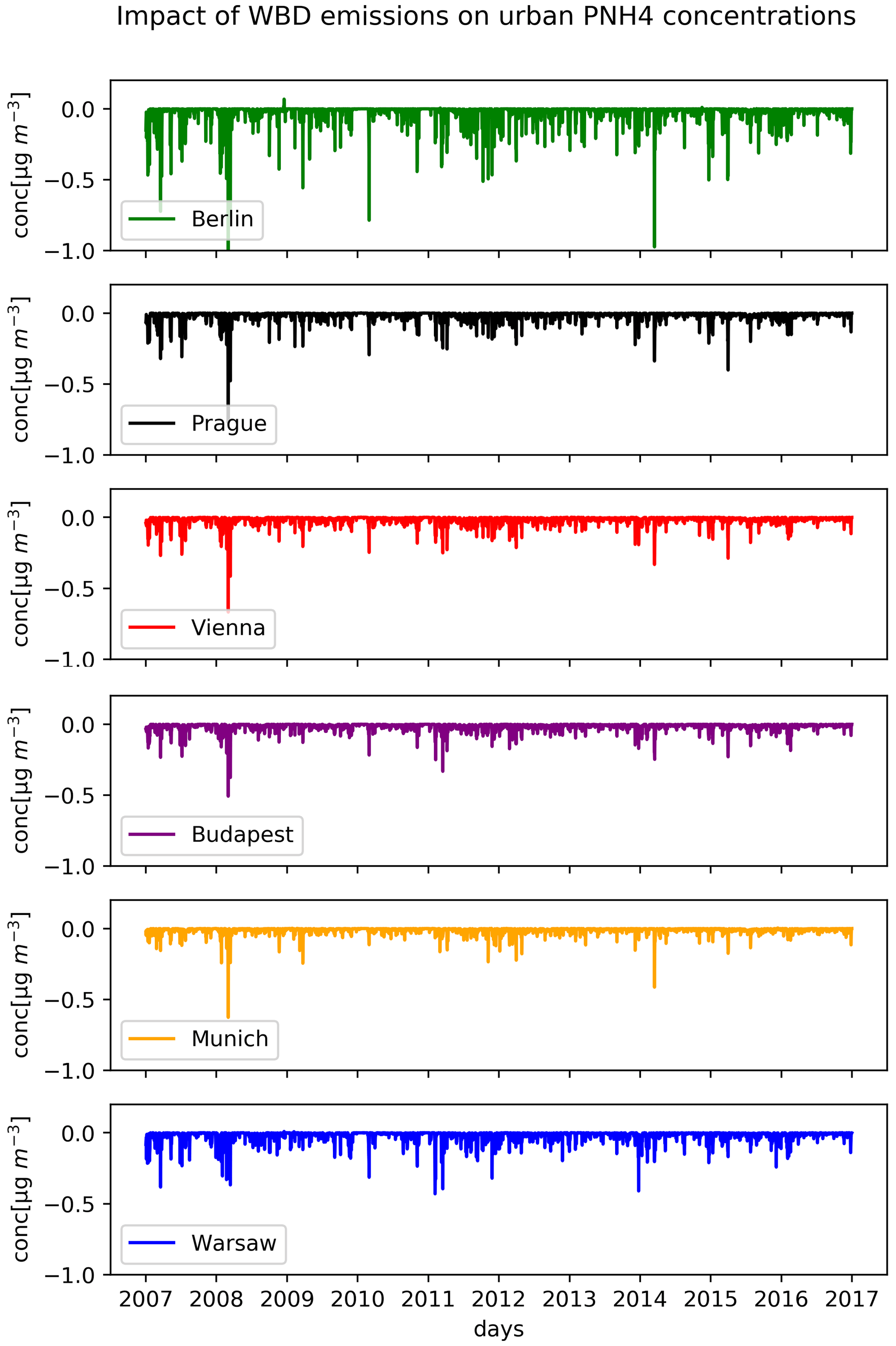
Figure 25 The long-term WBD impact on PNH₄ concentrations in ISORROPIA, averaged daily for 2007–2016. Units are micrograms per cubic metre.

In contrast with the seasonal low impact of WBD on PSO₄ concentrations, daily extreme values show an impact of up to 0.5 µg m⁻³, while for some cities like Berlin, it is even higher than 1 µg m⁻³. These values usually occur during the cold part of the year in accordance with the spatial results presented earlier. The daily WBD impact on nitrates is shown to also be higher than the seasonal one, with values reaching 1–1.5 µg m⁻³. The WBD impact on ammonium seems to have a decreasing effect, with values ranging between −0.1 and up to −0.5 µg m⁻³, which is also significantly higher than the seasonal ones.

4 Discussion and conclusions

This study aimed at the potential long-term regional impact of dust emissions on PM_2.5 and PM₁₀ concentrations for the period 2007–2016. The analysis focused on central Europe and on big urban areas such as Berlin, Prague, Vienna, Munich, Budapest and Warsaw. The impact was also estimated for the secondary inorganic aerosol concentrations as constituents of PM_2.5.

In our simulations, the annual average coarse and fine PM emitted and averaged over the whole domain is about 1.5 and 0.5 $\mathrm{Mg}{\mathrm{yr}}^{-\mathrm{1}}{\mathrm{km}}^{-\mathrm{2}}$, so about 2 $\mathrm{Mg}{\mathrm{yr}}^{-\mathrm{1}}{\mathrm{km}}^{-\mathrm{2}}$ for the total PM₁₀. This value is 1 order of magnitude higher than that calculated by Korcz et al. (2008) for Europe. The dust emissions show significant temporal and spatial patterns. Our dust model computed 2 times stronger emissions during the winter period than in summer (for both the fine- and coarse-dust particles). Over high-latitude areas, Bullard et al. (2016) reported strong winter dust emissions over areas where, under dry conditions, the sublimation of snow (and eventually permafrost) occurs and the soil is more prone to saltation, while during summer, the soil is generally more moist reducing the saltation potential of soil particles. In the dust model used in this study, the three most important parameters affecting the dust emissions are the near-surface wind speed, snow-equivalent water and soil moisture. The reason for much higher winter WBD emissions can be (1) much higher modelled winter wind speeds compared to summer ones, lower soil moisture during the winter months and an underestimation of snow cover, which prevents dust events. We saw that our driving model (WRF) produced much higher winds than the ones measured, and this positive bias is largest during winter. This strong overestimation is a known feature of the BouLac planetary boundary layer (PBL) scheme used in this study, and others have reported a similar overestimation of wind speed (e.g. Tyagi et al., 2018; Zhang et al., 2021). As dust emissions scale non-linearly with wind speeds that are above a certain threshold (Duran et al., 2011), this raises the potential for overestimating dust emissions if winds are overestimated. Our sensitivity estimates confirmed this and, even at a 5 % reduction in model wind speeds, greatly reduced the calculated WBD fluxes. We must note too that by driving WRF with the newer ERA-5 reanalysis data (Hersbach et al., 2017) instead of ERA-Interim, some of the wind biases would probably be reduced as it has been shown by many (e.g. Belmonte Rivas and Stoffelen, 2019) that ERA-5 provides somewhat lower near-surface wind speeds over Europe compared to ERA-Interim.

Regarding the modelled soil moisture, it is comparable to observed values in winter and somewhat higher during other months than that measured. This means that the strong winter emissions are probably due to high wind speeds in WRF. The last factor potentially playing a role is the snow cover, which was not evaluated in this study, but the modelled precipitation exhibited some underestimation in winter, which might result in reduced snow in our simulations (even though temperature is underestimated in winter).

Apart from the clear annual cycle, the calculated emissions show a diurnal cycle too. Daytime emissions are usually 50 %–100 % higher than nighttime ones. The reason for this is most probably the well-known cycle of wind speed with maxima occurring at noon (Huszar et al., 2018, 2020), and similar diurnal behaviour of dust emissions were seen in other studies too (e.g. Klose and Shao, 2012).

The daily time series of dust emissions provide some hints regarding their distribution: while on most of the days, the coarse-mode emissions remain low (lower than 0.1–0.2 $\mathrm{g}{\mathrm{s}}^{-\mathrm{1}}{\mathrm{km}}^{-\mathrm{2}}$), on selected days the emissions peak at much higher values (1–2 $\mathrm{g}{\mathrm{s}}^{-\mathrm{1}}{\mathrm{km}}^{-\mathrm{2}}$). The same is true for the fine-mode dust. This points to the fact already mentioned that the dust emissions respond non-linearly to wind speeds (more specifically to friction velocity; see Eq. 2) above a certain threshold. As wind speeds are overestimated in the driving meteorological model (WRF), the emissions are probably also overestimated, or at least these strong peaks are not realistic. Indeed, the sensitivity analysis to wind speed reduction showed a very high sensitivity of WBD emissions to this parameter: making the wind speeds half of the original values removed almost all WBD emissions. This means that very accurate meteorological driving data are needed to constrain the wind-blown dust emissions. We can further expect that due to the positive wind bias and resulting overestimated WBD emissions, the actual dust emissions are closer to what Korcz et al. (2008) calculated.

One interesting feature is evident from the modelled geographical distribution of seasonal WBD emissions. Besides large rural areas emitting dust, the largest dust sources are concentrated near large urban areas: the Ruhr area in Germany, the highly populated Benelux states and also large cities like Berlin, Prague, Budapest, etc. One has to be very cautious in interpreting this result: dust is potentially emitted only over land use categories representing potentially bare soil (if other circumstances are met), i.e. crops, shrubs, grass land, tundra and desert. “Urban” land use is, however, not treated as having dust emission potential. On the other hand, urban areas are characterized by low vegetation and thus low leaf area index (LAI). Indeed, in the LAI data used (MODIS), cities have near-zero LAI for most of the year. As land use in the WBDUST module (and also for CAMx dry deposition) is represented as fractional land use (based on CORINE data), many of the 9 km grid boxes covering urban areas are partly covered with bare soil and partly urban land use. If the LAI value is too low for such areas, dust emission can occur in the model. This was the case for densely populated areas, e.g. over the above-mentioned Ruhr area. In the case of large cities, such as Berlin, dust emissions are concentrated near the edges of the city, where grid boxes share both urban land use and bare soil. Our sensitivity analysis of the way MODIS LAI is averaged over CAMx grid cells showed that if the lowest LAI values (assuming these constitute the urban fraction of the grid cell which cannot emit WBD) are omitted from the averaging, the resulting average LAI over the grid cell is much higher, making the average WBD emissions smaller. Thus, this has to be treated as a caution to provide consistent input data for land use and other land-related parameters like LAI, preferably with a similar horizontal resolution.

Regarding the PM concentrations, the background noWBD case showed a reasonable model performance with typical correlations for PM_2.5 and PM₁₀ as achieved in other modelling studies for Europe (e.g. Lecoeur and Seigneur, 2013; Tsyro et al., 2022). Lowest correlations are computed for the summer period, while winter ones are usually the highest. This can be explained by the more stable weather conditions in DJF, which are better resolved than summer weather, which is often marked with highly variable convective environment (Huszar et al., 2016). The PM values are underestimated in summer and overestimated in winter, which is probably due to vertical transport that is too strong in summer and transport that is too low in winter but may be connected also to deficiencies in the monthly profiles used for annual emissions (Huszar et al., 2018, 2020). An important goal of the model validation was to evaluate whether the inclusion of WBD emission improves model performance. This turned out to be true for summer biases, which were reduced by adding the dust load. However, the winter, which was already marked by a negative bias, is modelled with an even higher bias if dust is considered. Also, the correlations decreased significantly if wind-blown dust is included in our simulations. This can be explained by the strong peaks in the impact on PM values which are a result of strong emission peaks seen in the daily time series of FCRS and CCRS emissions. The modelled urban PM peaks are often much higher (often by a factor of 5 or even more) than measurements and thus can strongly reduce the correlation with the observed values. Also, the RMSE values increased, which can again be explained by the many outliers in the modelled PM data.

Similar to dust emissions, the WBD impact on overall PM concentrations is high near big urban centres (over Germany and the Benelux states; reaching 15–20 µg m⁻³), but large rural contributions are also modelled, exceeding 2 and 5 µg m⁻³ for PM_2.5 and PM₁₀, respectively. The contributions are largest when the largest emissions occur, and we showed an evident correlation of high concentrations of PM₁₀ with high emissions of WBD in the coarse model. These seasonally averaged impacts are, however, strongly exceeded by the daily average values, which can be higher by 1 order of magnitude, reaching 100 µg m⁻³ for some cities. However, as already said, these extreme peaks are probably overestimated (due to too strong winds in WRF).

Vautard et al. (2005) calculated the summer and autumn wind-blown dust contribution to PM due to European local sources and found a contribution of around 1–2 µg m⁻³ to PM₁₀ over central Europe, which is about 2 times less than in our simulations. We can, however, expect that our result would get closer to their numbers without the positive wind bias encountered in our driving model.

Apart from the impact on the overall PM${}_{\mathrm{2.5}/\mathrm{10}}$ concentrations, our study quantified the long-term impact on the secondary aerosol components, namely the secondary inorganic aerosol (SIA) components. On a seasonal average, the impacts are rather small: an up to around 0.1 µg m⁻³ increase for PSO₄ (mainly during winter) and PNO₃ (all year round). For PNH₄, we modelled decreases of a similar absolute magnitude. A much higher impact is, however, calculated for specific days as daily means. These can reach an increase of up to 0.5–1 µg m⁻³ for sulfates (maximum increase over Berlin in 2009 exceeding 1 µg m⁻³) and similar increases for nitrates. During winter 2008–2009, nitrates occasionally even decreased by up to 0.2–0.3 µg m⁻³. Ammonium decreased due to dust by up to −1 µg m⁻³ on selected days. These decreases occurred mainly on winter days.

The explanation of the above-presented SIA modifications can be explained by two types of processes: one is the heterogeneous oxidation from SO₂ and N₂O₅ on the surface of dust particles (Wang et al., 2012; Zheng et al., 2015), and the other is the catalytic oxidation enhancement by dust elements in cloud water through influencing cloud pH and thus the aqueous chemistry of SO₂, HNO₃ and NH₃. Indeed, if we consider the impact on total SIA, we see that SIAs increased (the increases in sulfates and nitrates outweigh the decrease in ammonium). This is in line with the expectation and with previous studies dealing with the impact of dust on secondary aerosol formation (Malaguti et al., 2015).

Concretely, the increases in sulfates due to the presence of dust particles were modelled by Wang et al. (2012) (increases by about 1 µg m⁻³ during a strong dust event in China), who attributed them to dust surface heterogeneous chemistry. Also, Kakavas and Pandis (2021) modelled increases in sulfates over Europe due to dust. Our findings are also in line, at least qualitatively, with the recent findings of Wang et al. (2022), who argued that on the “dust surface, heterogeneous drivers (e.g. transition metal constituents, water-soluble ions) are more efficient than surface-adsorbed oxidants (e.g. H₂O₂, NO₂, O₃) in the conversion of SO₂, particularly during nighttime”.

Regarding the impact on nitrates, the increases are consistent with an earlier study of Fairlie et al. (2010), who found that nitrates associate with dust and result in volatilization. The increase in nitrates can be explained also by the formation of deliquescent salts (e.g. through the reaction of crustal cations in dust with NO³⁻ ions), as argued also by Wang et al. (2012). This can potentially even lead to some overprediction of nitrates, which requires revisiting the chemical composition of dust (Karydis et al., 2011).

Finally, the ammonium response to dust is tightly connected to the response of sulfates and nitrates. As we saw that nitrates easily associate with dust (via reaction with dust crustal anions like Ca²⁺), this means that less nitrate is available to react with ammonium, leading to more ammonia remaining in the gas phase (Fairlie et al., 2010). In other words, NH4⁺ is replaced by dust containing cations (Wang et al., 2012). This last author and others (e.g. Malaguti et al., 2015) note that ammonium could also increase due to the present of dust as a result of more sulfates forming on dust surfaces. However, in our simulations this is evidently offset by the above-mentioned replacement of ammonium by crustal cations.

In our experiments, the impact on SIA is clearly stronger using EQSAM, although the differences are not large and the overall impact on PM is not affected too much. The reason for stronger sulfate and nitrate formation in EQSAM is probably the fact that in EQSAM, the cloud pH is influenced by three cations (Mg${}^{++}$, Ca${}^{++}$ and K⁺), while in ISORROPIA, it is only influenced by calcium. This also explains the stronger decrease in ammonium in EQSAM being replaced by more cations.

An exception to the above-mentioned behaviour for nitrates is the winter 2009 decrease (by about 0.2 µg m⁻³) seen for all analysed cities. This period is not characterized by exceptional dust emissions or extreme PM values (based on our results). On the other hand, during this period, the dust impact on PSO₄ is relatively large, while the impact on ammonium is very small. Thus ammonium was probably preferably neutralizing sulfates instead of nitrates, causing their reduction.

Summing up the results, we showed that the long-term impact of local wind-blown dust emissions in Europe can significantly enhance urban PM levels, especially during extreme events rather than in seasonal averages. However, our calculations probably overestimate dust emissions due to very strong winds in the driving model. We also showed that apart from the total aerosol load, dust also impacts the secondary inorganic fraction of PM, which can significantly increase on selected days.

We also have to note that the uncertainties related to different inputs used for the study cannot be judged well here. We already mentioned that the land use and the LAI input can coact (bare soil vs. low or high LAI) differently depending on the choice of these data. For example, this led to one of the highest dust emissions in our simulations being located around urban areas. We also used some default values for dust composition based on a study (Karydis et al., 2011) which measured this composition over a different geographic area. Lastly, we used only one driving model and one model for wind-blown dust emissions, so the model uncertainty also cannot be addressed. The future goal should thus be to focus on the sensitivities of wind-blown dust loads to different input data and methods to obtain a more robust long-term estimate of dust emissions and the impact on PM and its secondary components.