Surface-based observations of cold-air outbreak clouds during the COMBLE field campaign

Cold-air outbreaks (CAOs) are characterized by extreme air–sea energy exchanges and low-level convective clouds over large areas in the high-latitude oceans. As such, CAOs are an important component of the Earth's climate system. The CAOs in the Marine Boundary Layer Experiment (COMBLE) deployment of the US Department of Energy Atmospheric Radiation Measurement (ARM) Mobile Facility (AMF) provided the first comprehensive view of CAOs using a suite of ground-based observations at the northern coast of Norway. Here, cloud and precipitation observations from 13 CAO cases during COMBLE are analyzed. A vertical air motion retrieval technique is applied to the Ka-band ARM Zenith-pointing Radar (KAZR) observations. The CAO cumulus clouds are characterized by strong updrafts with magnitudes between 2–8 m s⁻¹, vertical extents of 1–3 km, and horizontal scales of 0.25–3 km. A strong relationship between our vertical air velocity retrievals and liquid water path (LWP) measurements is found. The LWP measurements exceed 1 kg m⁻² in strong updraft areas, and the vertical extent of the updraft correlates well with the LWP values. The CAO cumulus clouds exhibit eddy dissipation rate values between 10⁻³ and 10⁻² m² s⁻³ in the lowest 10 km of the atmosphere, and using a radar Doppler spectra technique, evidence of secondary ice production is found during one of the cases.

1 Introduction

The Arctic is experiencing warming at the surface and throughout the troposphere at a rate faster than the rest of the world, a phenomenon known as Arctic amplification (AA; Previdi et al., 2021). The warming signal correlates in time and space with areas of significant sea-ice loss (Dai et al., 2019). Representing AA in climate simulations requires a comprehensive understanding of the different climate feedbacks and their impact on Arctic amplification, which include the Planck response and changes in water vapor plus temperature lapse rate, surface albedo, and clouds (Forster et al., 2021). Not surprisingly, the cloud feedback is particularly challenging to quantify (Zelinka et al., 2020). The latest Intergovernmental Panel on Climate Change (IPCC) assessment report found low confidence that the Arctic cloud feedback is positive, and it may even be slightly negative (Forster et al., 2021). Using reanalysis and satellite data, Zhang et al. (2018) indicated a large uncertainty in the sign of the Arctic cloud feedback. An improved understanding of high-latitude cloud systems, especially those over the open ocean such as cold-air outbreaks (CAOs), is needed since AA is connected to greater sea-ice loss.

CAOs occur when cold, dry air is transported over the relatively warm ocean, where the ocean surface can then release large amounts of heat and moisture into the air (Pithan et al., 2018). Climatological studies have highlighted the frequency at which CAOs occur in the Northern Hemisphere (Kolstad et al., 2009; Kolstad, 2011; Fletcher et al., 2016a, b; Smith and Sheridan, 2020), while others have focused on the Arctic region specifically. Papritz and Spengler (2017) found that a high frequency of CAOs occur in the Irminger and Nordic seas while McCoy et al. (2017) found that December through February is the season of maximum occurrence for open mesoscale cellular clouds, typical of CAOs, in the Norwegian Sea. Brümmer and Pohlmann (2000) also found that, across 10 winters, organized convection in CAO events occurs more than 50 % of the time over the Greenland and Barents Sea regions. Most of these analyses are limited to reanalysis and satellite datasets, and more observational work is crucial to our understanding of CAOs.

Early observational analyses of CAOs have focused on aircraft and sounding data from various field campaigns around the globe (Lau and Lau, 1984; Hein and Brown, 1988; Chou and Ferguson, 1991; Brümmer, 1996, 1997, 1999; Renfrew and Moore, 1999). Recently, work has been done on data from the ACTIVATE (Aerosol Cloud meTeorology Interactions oVer the western ATlantic Experiment) and ACCACIA (Aerosol–Cloud Coupling And Climate Interactions in the Arctic) field campaigns that managed to capture some CAO events (Young et al., 2016; Seethala et al., 2021; Tornow et al., 2021), although studying CAOs was not the main goal of the campaigns. The MPACE (Mixed-Phase Arctic Cloud Experiment) field campaign also provided opportunity for ground-based observations of CAO events in Alaska (Shupe et al., 2008). However, there are other regions in the Northern Hemisphere where ground-based observations of CAOs are lacking. Despite the importance of CAO clouds, high-resolution dynamical and microphysical observations, especially from surface-based remote sensing facilities in the regions of Greenland and the Norwegian Sea where models exhibit large inconsistencies, are not available (Pithan et al., 2014; Tomassini et al., 2017).

Here, analysis of surface-based observations from the Cold-Air Outbreaks in the Marine Boundary Layer Experiment (COMBLE) field campaign are presented. Initial work has been done using satellite data on two COMBLE cases (Wu and Ovchinnikov, 2022), and this study will also focus on measurements taken during the campaign. Using profiling Doppler cloud radar, lidar, and surface sensors, CAO events are identified, and the dynamical and microphysical properties of the shallow convective clouds during CAOs are described. Section 2 describes the COMBLE field campaign and the data used in this study. Section 3 describes the various data analysis methodologies used, including the retrievals of vertical air motion, eddy dissipation rate, and the detection of secondary ice production. Finally, we present our results in Sect. 4 and our conclusions in Sect. 5.

2 Data

From 1 December 2019 to 31 May 2020, the U.S. Department of Energy deployed the Atmospheric Radiation Measurement (ARM) first mobile facility (AMF1) near the Norwegian Sea for the Cold-Air Outbreaks in the Marine Boundary Layer Experiment (COMBLE) field campaign. The AMF1 was located on the northern coast of Scandinavia at a latitude of 69.141^∘ N, a longitude of 15.684^∘ E, and an altitude of 2 m above sea level, while a smaller set of instruments were deployed at a latitude of 75^∘ N on Bear Island. The main objective of the experiment was to quantify the properties of shallow convective clouds that develop as part of an air-mass transformation process when cold air advects over open water (Geerts et al., 2021). The two sites were located south of the Arctic ice edge, and the instruments successfully gathered comprehensive measurements of atmospheric conditions, clouds, precipitation, and aerosol that are used in this study.

The main instrument used in this study is the Ka-band ARM Zenith-pointing Radar (KAZR, Kollias et al., 2016), a zenith-pointing Doppler cloud radar operating at 35 GHz. The KAZR has a vertical resolution of 30 m and a temporal resolution of 2 s (Kollias et al., 2020). In this study, the radar reflectivity factor and mean Doppler velocity from the general mode are used. For polarimetry, we supplement our dataset with Doppler spectra observations from the collocated Ka-band ARM Scanning Cloud Radar (Ka-SACR, Kollias et al., 2014a) during times of vertically pointing operation. The Ka-SACR has a vertical resolution of 49.96 m and a temporal resolution of 2.97 s. Liquid water path (LWP) estimates were provided by a microwave radiometer (MWR) that operates at 23.8 and 31.4 GHz to determine column-integrated water vapor and liquid water along the vertical line-of-sight path (Morris, 2006). The balloon-borne sounding system (SONDE), in which soundings are launched every 6 h, and the Interpolated Sonde (INTERPSONDE) value-added product are used to retrieve profiles of atmospheric conditions over AMF1 (Holdridge, 2020; Jensen and Toto, 2016). The eddy dissipation rate (EDR; Borque et al., 2016) retrievals use the horizontal wind variables from INTERPSONDE as inputs, and the updraft width (chord length) calculations use the horizontal wind variables from SONDE. For the cloud base height (CBH) data, we use a Vaisala laser ceilometer, which sends a laser pulse at a 910 nm wavelength to detect light scattered by clouds and precipitation (Morris, 2016). Finally, to understand the type of precipitation reaching the surface at AMF1, we use a PARSIVEL2 laser disdrometer (Bartholomew, 2020). The PARSIVEL 1 min particle size distributions and fall velocities were used to characterize the precipitation type and intensity.

3 Methodology

3.1 CAO events selection

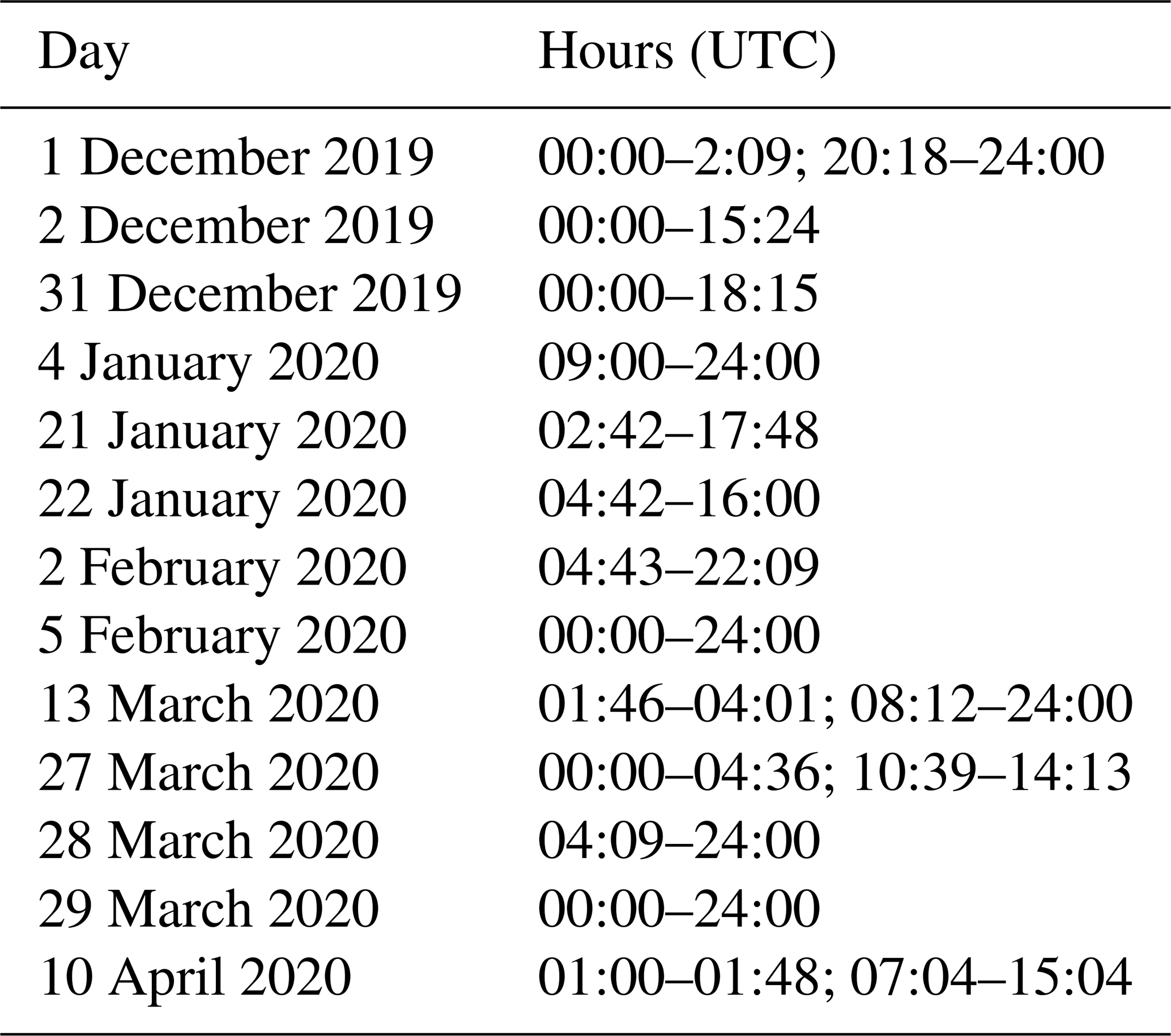
During the COMBLE field campaign, 34 CAO days were identified over the 6-month period for a total of 19 % of the campaign (Geerts et al., 2022). Here, data from 13 of these days are used. All periods with prefrontal and frontal cloud systems are removed, and our analysis focuses on the dynamical and microphysical characteristics of the periods with shallow convective CAO clouds. The cases and time periods are listed in Table 1.

Table 1 Dates and times used from the COMBLE field experiment.

3.2 Vertical air motion retrieval

The KAZR mean Doppler velocity (V_D) contains contributions from the vertical air motion (V_AIR) and the reflectivity-weighted particle sedimentation velocity (V_SED). The estimation of V_AIR requires the removal of V_SED from the observed V_D (Kollias et al., 2022; Zhu et al., 2020). Well-established techniques applicable to profiling Doppler cloud radar observations (Protat and Williams, 2011; Kalesse and Kollias, 2013) exist that can provide adaptive relationships between V_SED and radar reflectivity factor (Z). These relationships have been evaluated in stratiform precipitation systems where the V_AIR is weak, and its mean value is near zero averaged over a 20 min or longer period. Lamer et al. (2015) indicate that such relationships are challenging to develop in cumulus clouds due to the preferential presence of strong updraft motions. The presence of updrafts will bias low (reduce) the hydrometeor size distribution V_SED and can, in many cases, result in positive (upward) hydrometeor motion. A preliminary visual inspection of the KAZR and MWR CAO observations indicated that strong updraft motions indicated by the positive KAZR Doppler velocity measurements (V_D>2 m s⁻¹) are usually during periods when the MWR indicated the presence of high values of LWP. A LWP threshold of 0.25 kg m⁻² was selected to identify these periods. The selected periods have very little sensitivity to the selected LWP threshold. Here, we use the apparent relationship between LWP and V_AIR by filtering out all KAZR observations when the LWP exceeded 0.25 kg m⁻². All other KAZR observations are used to estimate the relationship between V_SED and Z using the methodology proposed by Protat and Williams (2011). To confirm our choice of LWP threshold, we found the relationship between V_SED and Z below cloud base for all 13 cases in both the high (>0.25 kg m⁻²) and low (<0.25 kg m⁻²) LWP periods. The relationships were very similar (not shown), meaning similar types of particles are falling below the cloud base in both regions.

First, the KAZR signal-to-noise ratio (SNR) values are used to identify the locations of hydrometeors using the Hildebrand and Sekhon (1974) threshold technique (Kollias et al., 2014b). The KAZR observations during periods with LWP < 0.25 kg m⁻² are sorted into reflectivity bins with widths of 1.5 dB in the range of −20 to +20 dBZ. In each reflectivity bin, the corresponding V_D are used to estimate the median Doppler velocity. The median Doppler velocity is our best estimate (BE) of the V_SED,BE for the radar reflectivity values within a particular bin. Reflectivity bins that contain less than 1 % of the KAZR observations are discarded due to their small sample size. The bin pairs of radar reflectivity and corresponding V_SED,BE create a look-up table (no fit is attempted), and this process is repeated for each CAO case. Figure 1a shows the Doppler velocity box plots for each reflectivity bin on 28 March; the other 12 CAO cases (not shown) exhibit a similar behavior. Despite this, we do not create a global Z–V_D look-up table; rather, each day's data are used to capture the smaller difference unique to the day. Sensitivity tests for these fits are performed using two other LWP thresholds of 0.5 and 0.8 kg m⁻², and we found that once we exceeded 0.25 kg m⁻², the convective updrafts began influencing the Z-V_D relationships, supporting this threshold's ability to isolate the convection. Figure S1c and e in the Supplement show the median V_D values in the higher reflectivity bins approaching and even exceeding zero. Also noteworthy is that the median V_D values in Fig. S1a and b are similar, while the ones in Fig. S1c, d and e, f are not, reinforcing our choice of LWP threshold.

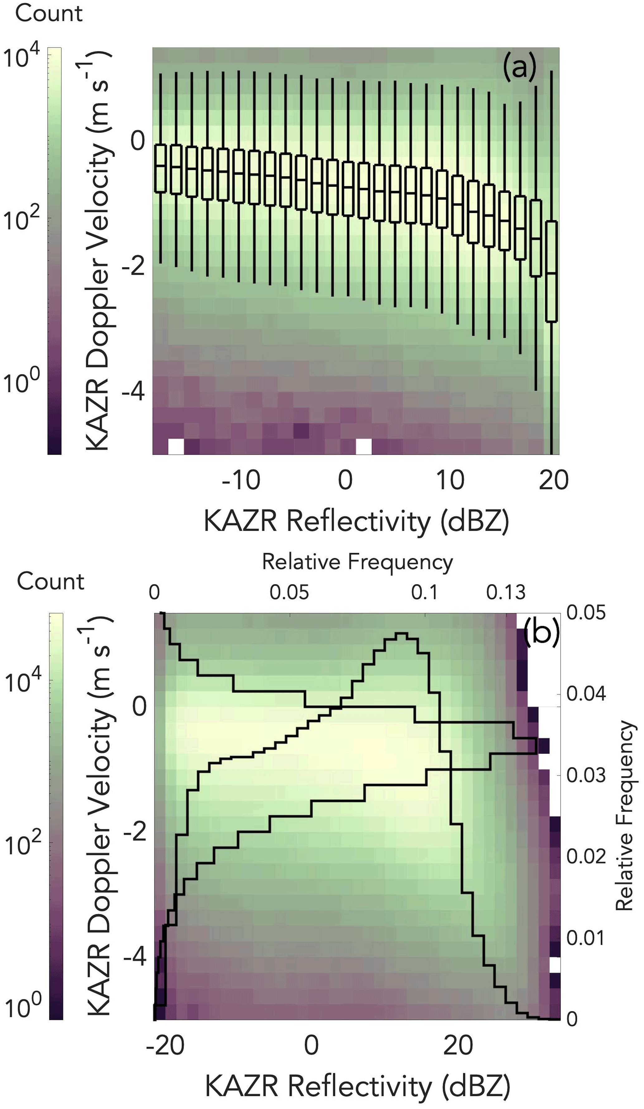
Figure 1 (a) For 28 March 2020, a joint probability density function (PDF) of KAZR reflectivity and Doppler velocity in the vertical profiles with a liquid water path (LWP) value less than 0.25 kg m⁻² and box-and-whisker plots showing the median Doppler velocity in every 1.5 dB reflectivity bin. (b) For all 13 COMBLE cases, a joint PDF of KAZR reflectivity and Doppler velocity in the vertical profiles with a LWP value less than 0.25 kg m⁻², the relative frequency distribution of KAZR Doppler velocity in the same low LWP periods, and the relative frequency distribution of KAZR reflectivity in the same low LWP periods. Prepared using Crameri (2021).

The V_SED,BE values in Fig. 1a are between 0.5–2 m s⁻¹, which is consistent with the presence of frozen hydrometeors. The relationship between the V_SED,BE and KAZR radar reflectivity indicates a gradual increase in the sedimentation velocity with radar reflectivity. The joint distribution of the KAZR radar reflectivity and V_D for all 13 CAO cases is shown in Fig. 1b. The KAZR radar reflectivity shows a broad distribution with most echoes between ±20 dBZ. The KAZR V_D distribution is centered at 0.5–0.75 m s⁻¹. For each CAO event, the relationship between radar reflectivity and V_SED,BE is used to estimate the vertical air motion V_AIR using the following expression:

$$\begin{array}{}\text{(1)}& V_{\mathrm{AIR}}\left(Z\left[t,h\right]\right)=V_{\mathrm{D}}\left(Z\left[t,h\right]\right)-V_{\mathrm{SED},\mathrm{BE}}\left(Z\left[t,h\right]\right),\end{array}$$

where t is time and h is height (range) of the KAZR observations. The uncertainty in the V_AIR estimates is controlled by the uncertainty of the V_SED,BE estimates since the primary measurement (V_D) has negligible uncertainty (below 0.15 m s⁻¹). The uncertainty of the V_SED,BE is controlled by the number of samples used in the estimation of the median V_D value within each radar reflectivity bin and the variability of the cloud microphysics during the sampling period. The V_SED,BE estimates for the same radar reflectivity bin differed very little from one CAO case to another (<0.25 kg m⁻²). The same uncertainty was found when shorter time periods were used. Using a fairly conservative approach, the uncertainty of the V_SED,BE is between 0.3–0.4 m s⁻¹.

During COMBLE, there were periods when the Ka-band Scanning ARM Cloud Radar (Ka-SACR, Kollias et al., 2014a, b) was pointing vertically. During these periods, the Ka-SACR recorded co- and cross-polar radar Doppler spectra, where the radar Doppler spectrum represents the frequency (velocity) distribution (spectral density, mm⁶ m⁻³ $/$ m s⁻¹) of the background radar signal at a particular range. In a vertically pointing radar, the Doppler spectra provide the distribution of backscattered signal, and the backscattered signal's intensity is controlled by the hydrometeor's number concentration and size over a range of Doppler velocities. These velocities are dependent on the hydrometeor's sedimentation velocity and the vertical air motion fluctuations within the radar sampling volume. The cross-polar Doppler spectrum provides information about the location (velocity) of non-spherical particles. The recorded co- and cross-polar radar Doppler spectra can be used as input to a novel retrieval technique that identifies the presence of secondary ice production (SIP) in supercooled mixed-phase clouds (Luke et al., 2021). V_AIR is estimated from the radar Doppler spectra using the location (in m s⁻¹) of the slower falling edge of the supercooled liquid spectral density's principal peak and is adjusted by a value of 0.28 m s⁻¹ to compensate for turbulence broadening. The selected velocity adjustment for turbulence broadening of the radar Doppler spectra is applicable only to radars operating with similar characteristics to the ARM KAZRs. The value of the “climatological correction” is based on a multi-year analysis of KAZR observations in mixed-phase and liquid clouds (Luke et al., 2021; Zhu et al., 2022). Our primary measurements in this analysis are linear depolarization ratio (LDR) determined by the ratio of the cross-polarized to co-polarized spectral density, calibrated co-polarized spectral reflectivity normalized to units of dBZ $/$ m s⁻¹, and spectral terminal fall speed computed as the difference between V_AIR and spectral V_D.

3.3 Eddy dissipation rate retrieval

EDR is retrieved from the KAZR Doppler velocity and the INTERPSONDE sounding product using the algorithm outlined by Borque et al. (2016). The INTERPSONDE sounding product is first interpolated to 2 s–30 m resolution to be consistent with the KAZR observations. For clouds with durations of less than 20 min, Doppler velocities for all the collected cloud profiles are used to generate the corresponding velocity power spectrum (S(f)) by performing a fast Fourier transform (FFT). Assuming the turbulence to be homogeneous, in the region of the inertial subrange, the EDR can be estimated as

$$\begin{array}{}\text{(2)}& \mathit{\epsilon }={\displaystyle \frac{\mathrm{2}\mathit{\pi }}{V}}\left\{{\displaystyle \frac{\mathrm{2}}{\mathrm{3}\mathit{\alpha }}}\underset{f_{\mathrm{1}}}{\overset{f_{\mathrm{2}}}{\int }}S\left(f\right)\mathrm{d}f\right\}(f_{\mathrm{1}}^{-\mathrm{1.5}}-f_{\mathrm{2}}^{-\mathrm{1.5}}{)}^{-\mathrm{1.5}},\end{array}$$

where ε is the retrieved EDR, V is the horizontal wind obtained from the sounding product, α is the Kolmogorov constant and is taken as 0.5, and f₁–f₂ is the lower and upper frequency limit in the inertial subrange. It is apparent that the accuracy of the ε retrieval is highly dependent on the selection of the inertial subrange, which is determined by the frequency interval (f₁–f₂). Here, we adapt the same approach proposed by Borque et al. (2016) to confine the inertial subrange: 33 frequency pairs are predefined for each selected frequency interval, a power law fitting is performed for the velocity spectrum S(f), and only the fitting slopes within $-\mathrm{5}/\mathrm{3}\pm \mathrm{1}/\mathrm{3}$ are selected as “good inertial subranges” and used for ε estimation. Finally, the retrieved ε from all the “good intervals” are averaged to obtain the ε product.

3.4 Updraft dimensions

The V_AIR retrievals are used to estimate properties of coherent updrafts in CAOs. A conditional threshold of V_AIR>2 m s⁻¹ is used to identify spatially coherent updraft structures. The 2 m s⁻¹ conditional velocity threshold is much higher than the V_AIR uncertainty (0.3–0.4 m s⁻¹). This will ensure that we detect the presence of an updraft. In addition, the 2 m s⁻¹ V_AIR threshold ensures we exceed the typical vertical air motion values observed in stratus and stratocumulus (Guibert et al., 2003; Peng et al., 2005; Guo et al., 2008; Ghate et al., 2010; Hudson and Noble, 2014). Using the algorithm outlined in Kollias et al. (2014b), a low-pass filter that is five vertical profiles wide and five range gates deep is applied to the V_AIR estimates three times. This allows for the identification of coherent updraft structures.

The coherent updraft structures are then analyzed to estimate their depth (vertical extent), width (chord length), and range of magnitudes within the structure. The distance between the lowest and highest KAZR range gates that a coherent updraft occupies is used to estimate their vertical extent. A similar approach is used to estimate the temporal duration of the updraft structures. This duration value is then multiplied by the average horizontal wind speed in the lowest 5 km of the atmosphere from the nearest sounding in time to give the chord length of the updraft. Finally, the range of magnitudes is given by all the values within the same coherent updraft structure. A sensitivity analysis was performed to evaluate the impact of the selected threshold for determining coherent updraft structures. Using a conditional threshold of V_AIR>1 m s⁻¹, we found negligible differences in the updraft statistics. Finally, due to a lack of soundings, 1 December only contributes to updraft vertical extent and magnitude results.

4 Results

An example 3 h period of CAO observations from 28 March 2020 is shown in Fig. 2. Several cumulus clouds were detected by the KAZR with cloud tops between 3.5 to 4.5 km. The surface temperature averaged 0.76 ^∘C for the period and never dropped below 0 ^∘C; meanwhile, temperatures ranged from −44.6 to −37.5 ^∘C near the cloud top, where we took the cloud tops to be the last detectable echoes in the KAZR columns. Within the region from the surface to the range of cloud tops, the lapse rate was about 8.4 ^∘C km⁻¹, and the prevailing wind was predominantly from the northwest with at most 8–9^∘ of wind shear. In COMBLE, the KAZR was operated only in co-polar mode. The lack of KAZR linear depolarization ratio observations prevents us from reliably using radar Doppler spectra techniques for a hydrometeor phase classification (Kalesse et al., 2016; Luke et al., 2021). No melting layer signature is detected in the KAZR radar reflectivity and mean Doppler velocity observations (Fig. 2b) throughout the observing period. The KAZR reflectivity exceeds +25 dBZ in the shallow convective cores, indicating the presence of large hydrometeors or a high number concentration. The retrieved V_AIR is shown in Fig. 2c. Several deep updraft structures are observed within the same shallow convective cloud suggesting the presence of boundary layer organization. In particular, the cumulus cloud detected around 10:00 UTC/11:00 LT exhibits four distinct updrafts with V_AIR values higher than 5 m s⁻¹. Similar coherent updraft structures are commonly observed throughout the COMBLE dataset. On the other hand, there are cumulus clouds with negligible or no updraft structures; this is a result of sampling clouds at different stages of their evolution. The MWR detected the presence of significant LWP (exceeding 1 kg m⁻²) in the areas where updrafts were retrieved. The collocation of the updraft structures with the presence of supercooled liquid provided confidence in the V_AIR estimates. Finally, the shallow convective clouds exhibit high EDR estimates reaching values of up to 0.01 m² s⁻³. Similarly with the presence of updrafts, the EDR values are higher in the areas of active shallow convective clouds (Fig. 2d).

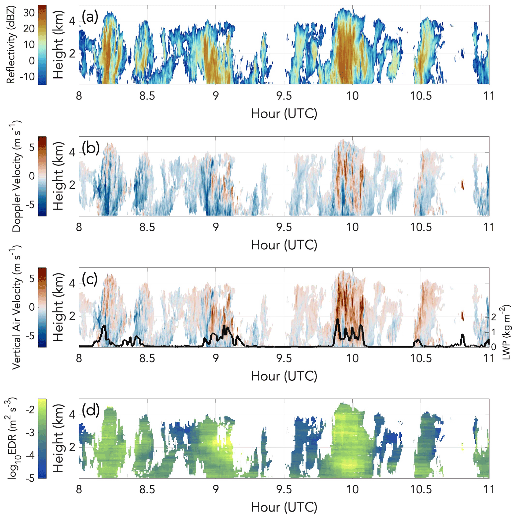
Figure 2 Time–height mapping from 08:00–11:00 UTC on 28 March 2020 of (a) KAZR radar reflectivity, (b) KAZR Doppler velocity, (c) retrieved vertical air velocity and liquid water path, and (d) retrieved eddy dissipation rate. Prepared using Crameri (2021).

4.1 Updraft structure analysis

One of the main scientific drivers of the COMBLE field campaign is to better understand mixed-phase cloud processes and improve their representation in high-resolution numerical models (Geerts et al., 2022). In-cloud updrafts are very important in microphysics. The observed distribution of updraft chord length from all CAO cases is shown in Fig. 3a. The distribution peaks at updraft chord lengths less than 500 m, and more than 80 % of the observed updrafts have chord lengths less than 1 km. Similarly, the observed distribution of updraft vertical extent peaks at a value less than 500 m. About 5 % of the observed updrafts have vertical extents higher than 1 km. The distribution of the range of updraft magnitudes (Fig. 3c) shows that most of the updrafts are defined by V_AIR values between 2 and 3 m s⁻¹, but some have values as high as 8–9 m s⁻¹. These values far exceed the ones found by Brümmer (1999) in aircraft data from the ARKTIS field campaign over the same region.

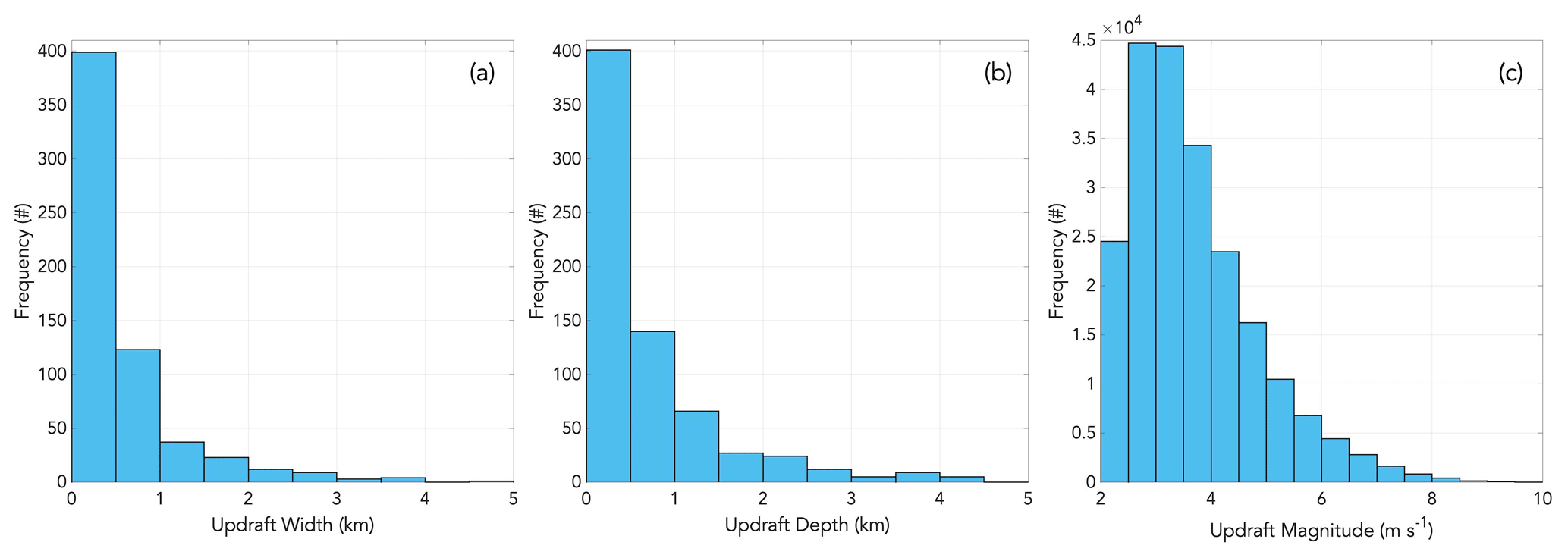
Figure 3 For all 13 COMBLE cases, histograms of (a) updraft chord length (width) in km, (b) updraft vertical extent in km, and (c) the range of magnitudes in the updraft in m s⁻¹.

The observed scales of CAO cumulus updrafts are unresolved by current global cloud-resolving models (Satoh et al., 2019). Since the KAZR data have such a high temporal resolution, we transform the KAZR time–height data to horizontal distance–height data using the mean horizontal wind speed from the lowest 5 km of the atmosphere from the nearest soundings in time. This allows us to look at the updraft chord length and magnitude at different horizontal resolutions: 250 m in Fig. 4a and c and 1 km in Fig. 4b and d. We take the median KAZR profile over each distance interval, and we run our low-pass filter only once. As the horizontal resolution becomes coarser, KAZR identifies fewer updrafts, and they are losing their impressive magnitudes. We also attempted a 3 km resolution, but none of the updrafts were resolved. The 250 m resolution distributions still closely resemble those seen in Fig. 3, so increasing a model's resolution beyond 250 m will hinder its ability to resolve the structures in CAOs.

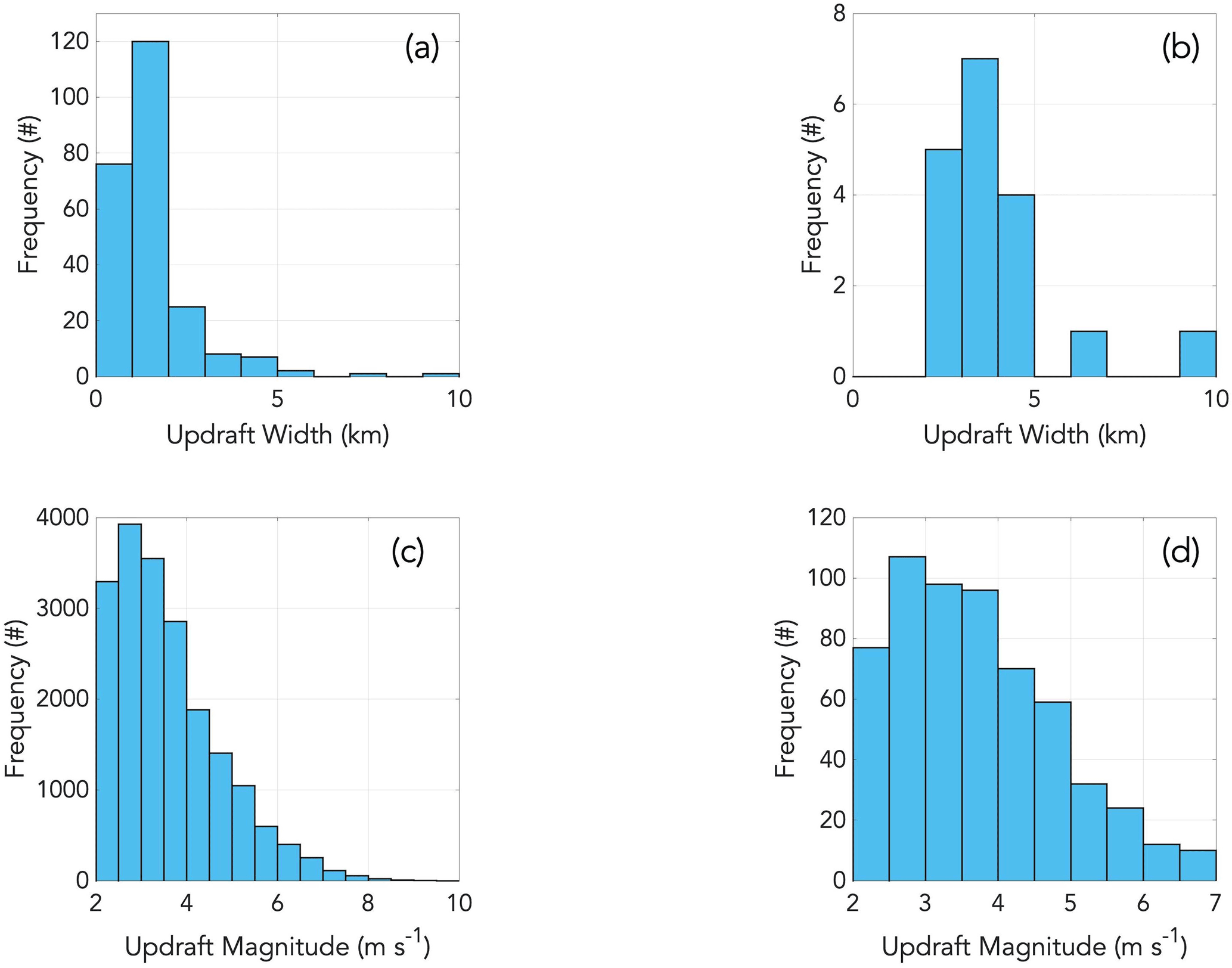
Figure 4 From all 13 COMBLE cases, histograms of updraft chord length (width) in km and range of magnitudes in the updraft in m s⁻¹ at a horizontal resolution of (a–b) 250 m and (b–d) 1 km.

We also examine the updraft magnitude profile as a function of normalized updraft depth. The observed updraft structures are classified into three categories of nearly equal size based on their vertical extent: those with depths less than 1 km (Fig. 5a), those with depths between 1 and 2 km (Fig. 5b), and those with depths greater than 2 km (Fig. 5c). In general, the deeper updrafts are associated with stronger vertical air motions. Throughout the normalized updraft depths, 55 % of V_AIR values are greater than 3 m s⁻¹ in Fig. 5a, 66 % of V_AIR values are greater than 3 m s⁻¹ in Fig. 5b, and 75 % of V_AIR values are greater than 3 m s⁻¹ in Fig. 5c. Finally, the whiskers in Fig. 5c show the deepest updrafts have both the strongest and weakest V_AIR values.

Figure 5 For all 13 COMBLE cases, box-and-whisker plots of updraft magnitude as a function of normalized updraft depth for (a) updrafts with a depth less than 1 km, (b) updrafts with a depth between 1 and 2 km, and (c) updrafts with a depth greater than 2 km.

4.2 EDR analysis

The distribution of the EDR measurements as a function of height above the surface for all CAO cases is shown in Fig. 6. The highest EDR values (10⁻³–10⁻² m² s⁻³) are observed near the surface. This is consistent with the strong surface sensible heat fluxes that characterize CAO cloud systems. At higher altitudes, the EDR distribution is broader. Two modes appear, one where the EDR steadily decreases with height and another where EDR stays constant with height. Overall, the strongest turbulence in the distribution is concentrated in the lowest 2 km between values of 10⁻³ and 10⁻² m² s⁻³. The two stratiform EDR profiles shown in Borque et al. (2016) do not share these characteristics. One does not have as deep of a layer as shown here, and the other has values closer to 10⁻⁴ m² s⁻³, 1 order of magnitude less than shown here.

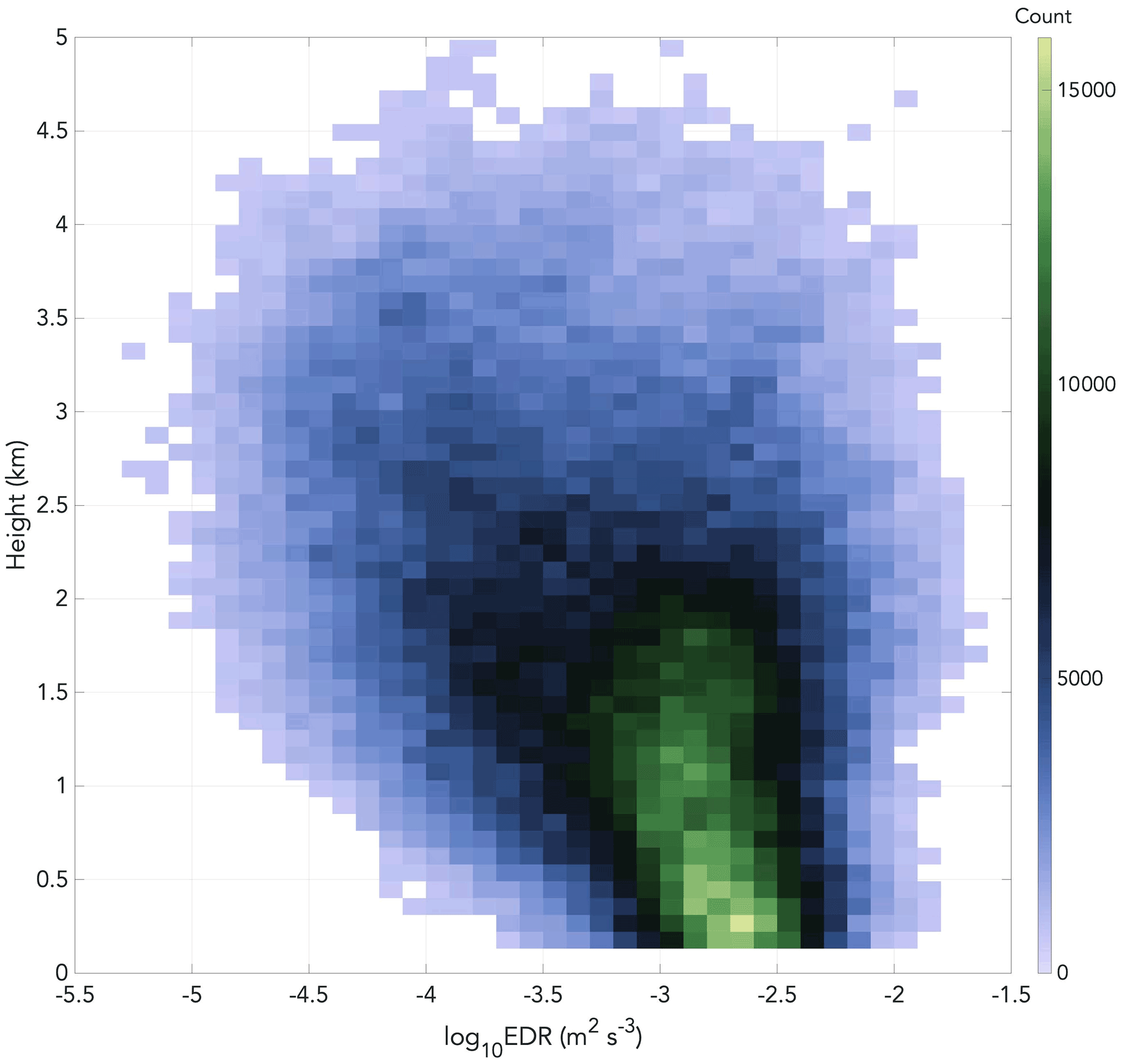
Figure 6 For all 13 COMBLE cases, a joint PDF of eddy dissipation rate versus height. Prepared using Crameri (2021).

4.3 Relationship between LWP and updrafts

Visual inspection of Fig. 2 suggests a correlation between the presence of liquid water and the coherent updraft structures. This relationship is further investigated using all the COMBLE observations (Fig. 7). Looking at the LWP measurements broadly, Fig. 7a shows nearly 75 % of the LWP data are near zero, while only about 1 % of the LWP data are higher than 2 kg m⁻². Meanwhile, Fig. 7b shows that as LWP in the column increases, so too does the maximum V_D, which reinforces the visual inspections we made and our use of LWP as a threshold for our vertical air motion retrieval. In general, the LWP correlates well with the square of the depth of the cloud (Wood, 2012; Yang et al., 2018). In Fig. 7c, the measured LWP is plotted against the sum of V_AIR values in the updraft depth. Similarly, in Fig. 7d, the LWP in the column is plotted against the maximum V_AIR value in the updraft depth. These two relationships exhibit a plausible agreement between two independent measurements, which further supports the good performance of the V_AIR retrieval technique.

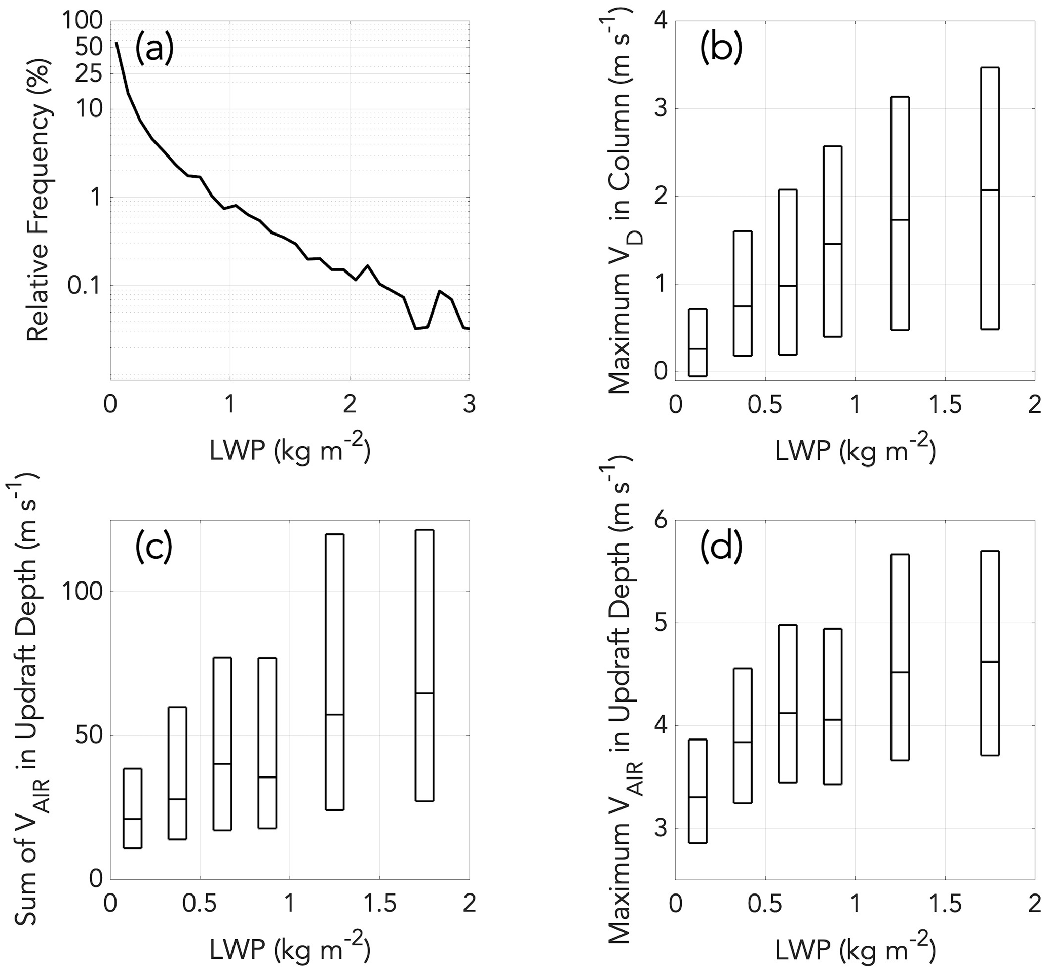
Figure 7 For all 13 COMBLE cases, (a) the relative frequency of liquid water path (LWP) in bins of width 0.1 kg m⁻²; (b) the median, 25th, and 75th percentile of the maximum Doppler velocity (V_D) in the atmospheric column for each LWP bin of width 0.25 kg m⁻² or 0.5 kg m⁻²; (c) the median, 25th, and 75th percentile of the sum of the vertical air velocity (V_AIR) in the updraft depth for each LWP bin of 0.25 or 0.5 kg m⁻²; and (d) the median, 25th, and 75th percentile of the maximum V_AIR in the updraft depth for each LWP bin of width 0.25 or 0.5 kg m⁻².

4.4 Hydrometeor fraction profile

Here, the relationship between updrafts and hydrometeor fraction profile is investigated. First, the KAZR data are separated into hour-long periods, and the hydrometeor fraction is calculated at each range gate. The hydrometeor fraction is the fraction of KAZR significant meteorological detections over the total number of KAZR profiles during the 1 h period. In addition, the updraft fraction is estimated as the fraction of retrieved V_AIR>2 m s⁻¹ over the total number of KAZR significant meteorological detections during the 1 h period. The distribution of the hourly estimated hydrometeor fraction as a function of normalized cloud height, where 0 represents cloud base and 1 represents cloud top, is shown in Fig. 8a. The maximum hydrometeor fraction gradually reduces towards the cloud top. The observed hydrometeor fraction profile suggests surface and cloud base conditions determine the overall cloud fraction in CAOs. No evidence of hydrometeor detrainment near the cloud top is observed, as it has been observed in the shallow oceanic convection (Lamer et al., 2015). The dataset is further classified into three CAO cloud thickness types by splitting it into three samples of nearly equal size: cloud top heights (CTHs) less than 3.5 km, CTHs between 3.5 and 4.5 km, and CTHs greater than 4.5 km (Fig. 8b). Despite their considerable differences in CTH, the hydrometeor fraction estimates near the cloud base are clustered around 0.52–0.6.

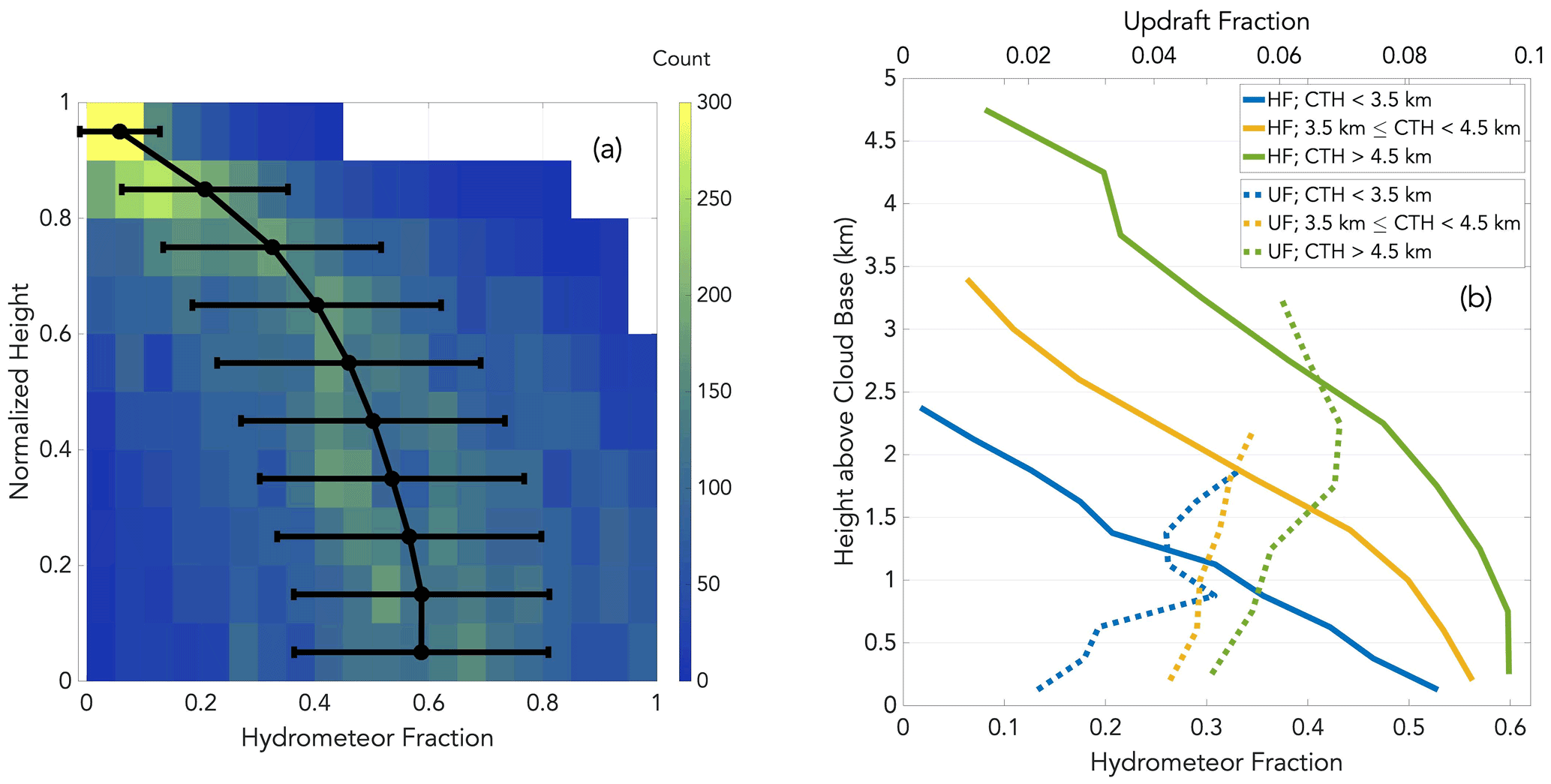
Figure 8 For all 13 COMBLE cases, (a) a joint PDF of hydrometeor fraction (HF) versus normalized height, along with a mean profile of HF as a function of normalized height and (b) mean profiles of HF (black) and updraft fraction (UF; blue) as a function of height above cloud base, with solid lines for cloud tops less than 3.5 km, dashed lines for cloud tops between 3.5 and 4.5 km, and dotted lines for cloud tops above 4.5 km. Prepared using Crameri (2021).

The updraft fraction profiles increase towards the cloud top (Fig. 8b). This is a combination of the updraft structures being vertically oriented and the overall hydrometeor fraction reduction with height above the cloud base. The mean updraft fraction near the cloud base for the three different CAO cloud top cases exhibit higher co-variability with CTH. The updraft fraction at the cloud base more than doubles between the shallow (CTH < 3.5 km) and the deep (CTH > 4.5 km) CAO cases. This further suggests that near the cloud base, conditions are important for determining the vertical extent of the CAO cumulus field.

4.5 Secondary ice production

The presence of strong updrafts and high supercooled liquid amounts within the temperature range of −3 to −8 ^∘C suggest the possibility for secondary ice production (SIP) within the CAO cumulus clouds. Luke et al. (2021) presents a comprehensive observational study that utilizes polarimetric radar Doppler spectra to detect and quantify the occurrence of SIP. The KAZR did not collect polarimetric observations during COMBLE, but the collocated Ka-band Scanning ARM Cloud Radar (Ka-SACR; Kollias et al., 2014a) spent time vertically pointing as part of its nominal sampling pattern. Using polarimetric radar Doppler spectra recorded by the Ka-SACR on 31 December 2019, we apply the method of Luke et al. (2021) to detect and quantify the occurrence of secondary ice production in the temperature range of −3 to −8 ^∘C. On that day, this temperature range extends from 500 to 1000 m in altitude (Fig. 9b). We detect the presence of Doppler spectra bin observations dominated by a columnar ice crystal habit by those having an LDR between −16 and −14 dB. We then aggregate these bins according to their terminal fall speed and divide their quantity by the total number of bins with a measurable LDR, aggregated in the same way by terminal fall speed. We require the co-polarized and cross-polarized spectral energy density to both be at least 4 dB above their noise floor for LDR to be measurable. We then know the fraction of hydrometeors that can be attributed to a columnar ice crystal habit as a function of terminal fall speed. Figure 9c shows that this fraction is enhanced at the altitude corresponding to a temperature of −5 ^∘C in the fall speed range of small needles. For comparison, we compute the fraction of Doppler spectra bins dominated by spherical hydrometeors as above by subsetting the numerator to observations having an LDR between −22 and −20 dB. As seen in Fig. 9d, minimal enhancement occurs near −5 ^∘C. Finally, following Luke et al. (2021), we determine the secondary ice multiplication factor of needle detections using the baseline detection threshold of −21 dBZ s m⁻¹, which is shown in Fig. 9e. Occurrences of secondary ice multiplications from 10× to 100× are readily apparent, with additional occurrences in the range of 100× to 1000×. Unfortunately, the Ka-SACR operations in a vertically pointing mode were not regularly executed, thus limiting our ability to conduct a comprehensive study of SIP detection and occurrence. Nevertheless, the one case analyzed clearly indicates the presence of SIP in CAOs.

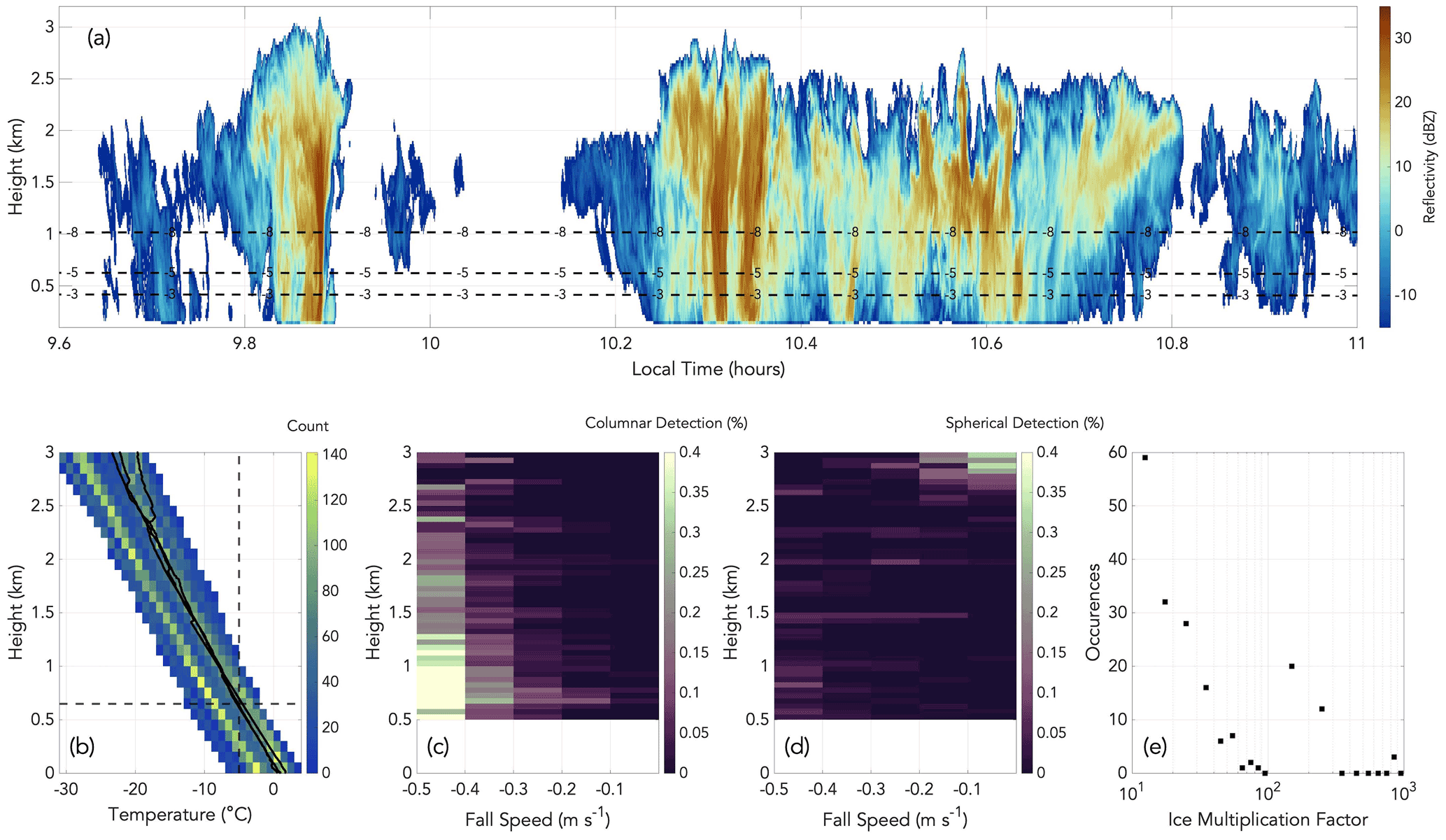
Figure 9 For 31 December 2019, (a) time–height mapping during 09:36–11:00 LT of KAZR radar reflectivity (colors) and INTERPSONDE isotherms (dashed black lines), (b) a joint PDF of temperature and height (colors) from 32 radiosondes launched during the 13 cases along with the three temperature profiles from 31 December (black), and the percentage of Doppler spectra with columnar detections (c) and spherical detections (d) in each fall speed–height bin during 00:00–18:15 LT. Prepared using Crameri (2021).

5 Conclusions

The COMBLE observations provide the first systematic long-term, cloud-scale, ground-based remote sensing dataset of Arctic CAOs. Observations from a profiling cloud radar (KAZR), a ceilometer, and a microwave radiometer (MWR) are used to study the cloud-scale dynamics of 13 CAO events. The KAZR observations are used to estimate CAO cumulus cloud properties such as hydrometeor fraction, cloud top height, vertical air motion, and EDR. The LWP measurements from the MWR and their relationship to cloud dynamics are investigated.

The CAO cellular shallow convective clouds observed at Andenes, Norway, have typical cloud top heights between 3 and 5 km, and the average hydrometeor fraction is 50 %–60 %. Owing to the large surface sensible heat flux, CAO cumulus clouds are characterized by strong updraft structures. The distribution of retrieved updraft magnitudes peaks at 3 m s⁻¹, but a considerable number of updrafts have vertical air motion values that exceed 4–5 m s⁻¹. On the other hand, the coherent updraft structures have narrow widths that peak at 250 m and vertical extents typically around 500 m. Representing these updraft structures in numerical models requires high-resolution modeling at the scales of 100–200 m horizontal spacing. The LWP time series indicates the intermittent presence of liquid columns with LWP values in excess of 1–2 kg m⁻². Furthermore, the intermittent spikes in LWP amount correlate with the detection of coherent updraft structures and their vertical extent. The EDR retrieval confirms the turbulent nature of the CAO cumulus clouds with the highest values near cloud base (∼ $\mathrm{5}\times {\mathrm{10}}^{-\mathrm{3}}$ m² s⁻³).

The CAO cumulus hydrometeor fraction profile peaks at the cloud base level (0.5–0.6) and gradually decreases with height above the cloud base. The cloud base hydrometeor fraction profile exhibits little relationship to the cumulus field cloud top height. On the other hand, the cumulus field cloud top height exhibits better covariance with the updraft fraction profile.

In addition, we show that secondary ice production is present during a cold-air outbreak, with ice multiplication factors approaching 3 orders of magnitude. This is consistent with a growing body of evidence suggesting that updraft regions containing supercooled liquid are favorable for secondary ice production.

The presented work provides valuable information for model intercomparison studies that will attempt to understand mixed-phase cloud processes in CAOs, but there is a limitation. Our work examines the cumuli from a Eulerian perspective and is restricted to a two-dimensional view of the atmosphere; we cannot speak to the evolution of the clouds nor to their three-dimensional geometry and organization. Future work may begin by looking at data collected by the Norwegian weather radar network and Ka-SACR during COMBLE, where one can analyze the mesoscale organization of the cumuli and their three-dimensional structure as they evolve in time.

Appendix A

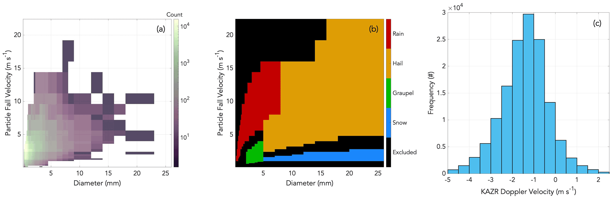
Figure A1 For all 13 COMBLE cases, (a) a joint PDF of disdrometer particle diameter and particle fall velocity, (b) a hydrometeor identification map used to categorize the precipitation type at the surface, and (c) a histogram of KAZR Doppler velocities at 300 m. Prepared using Crameri (2021).

The PARSIVEL2 disdrometer provides 1 min observations of hydrometeor size and fall velocity (Fig. A1a). The disdrometer observations have been successfully used in previous studies to classify the types (i.e., phase, density, size) of hydrometeors reaching the surface. Here, the PARSIVEL2-based hydrometeor identification developed by Friedrich et al. (2013a, b) and the size–velocity fits for unrimed particles in Locatelli and Hobbs (1974) are used to assess the hydrometeor typing in CAOs (Fig. A1b). Throughout the 13 cases, the rain hydrometeor type dominates, as it accounts for about 58 % of the total particles detected by the disdrometer (Fig. A1a). Hail, graupel, and snow only account for 0.52 %, 3.51 %, and 0.06 % of the total particles detected, respectively. The PARSIVEL2-based hydrometeor classification contradicts the KAZR observations. First, no noticeable attenuation is observed in the KAZR observations. Furthermore, the distribution of KAZR Doppler velocities at 300 m above the surface indicates that most of the values in the distribution are around 1.5 m s⁻¹ (Fig. A1c). The KAZR Doppler velocity measurements were compared against those recorded by the Ka-SACR. The comparison shows excellent agreement between the two radars. The discrepancy between the KAZR and disdrometer observations suggests the possibility of (i) artifacts in the disdrometer observations due to the orientation of the disdrometer and/or the near-surface wind magnitude and/or (ii) the presence of numerous irregularly shaped particles that are difficult to characterize using the disdrometer.