Boundary layer moisture variability at the Atmospheric Radiation Measurement (ARM) Eastern North Atlantic observatory during marine conditions

Boundary layer moisture variability at the Eastern North Atlantic (ENA) site during marine conditions is examined at monthly and daily timescales using 5 years of ground-based observations and output from the European Center for Medium range Weather Forecast (ECMWF) reanalysis model. The annual cycle of the mixed-layer total water budgets is presented to estimate the relative contribution of large-scale advection, local moisture tendency, entrainment, and precipitation to balance the moistening due to surface latent heat flux on monthly timescales. When marine conditions prevail, advection of colder and dry air from the north acts as an important moisture sink (∼ 50 % of the overall budget) during fall and winter driving the seasonality of the budget. Entrainment and precipitation contribute to the drying of the boundary layer (∼ 25 % and ∼ 15 % respectively), and the local change in moisture contributes to a small residual part. On a daily temporal scale, moist and dry mesoscale columns of vapor (∼ 10 km) are analyzed during 10 selected days of precipitating stratocumulus clouds. Adjacent moist and dry columns present distinct mesoscale features that are strongly correlated with clouds and precipitation. Dry columns adjacent to moist columns have more frequent and stronger downdrafts immediately below the cloud base. Moist columns have more frequent updrafts, stronger cloud-top cooling, and higher liquid water path and precipitation compared to the dry columns. This study highlights the complex interaction between large-scale and local processes controlling the boundary layer moisture and the importance of spatial distribution of vapor to support convection and precipitation.

1 Introduction

Marine boundary layer warm clouds cover vast areas of eastern subtropical oceans and persist for very long periods (Klein and Hartmann, 1993). These clouds reflect a much greater amount of radiation back to space compared to the ocean surface and hence are an important component of the Earth's radiation budget. It is challenging for earth system models (ESMs) used for predicting the future climate to accurately simulate these clouds as they, and the associated processes, occur at much smaller spatial and temporal scales than the model resolution.

Marine boundary layer stratocumulus and shallow cumulus are maintained by boundary layer turbulence through the transport of water vapor above the lifting condensation level. Some cloud parameterizations use the moments of the joint probability density functions (PDFs) of temperature, water vapor, and vertical air motion to simulate cloud properties. Hence changes in boundary layer water vapor critically impact cloud properties. Further the marine boundary layer clouds exhibit a distinct mesoscale organization (Wood and Hartman, 2006) with scales of 20–50 km. Recent modeling studies have shown that cloud and rain properties are organized in mesoscale structures and are closely related to changes in boundary layer water vapor (Zhou and Bretherton, 2019). Several modeling studies highlight the role of “mesoscale humidity aggregation” and its positive feedback in amplifying the moisture variance, cloudiness, and precipitation (Bretherton and Blossey, 2017; Lamaakel and Matheou, 2022).

To address scientific issues related to marine low clouds, the Atmospheric Radiation Measurement (ARM) Climate Research Facility (Mather and Voyles, 2013) operates the heavily instrumented Eastern North Atlantic (ENA) site located in the Azores archipelago. The location experiences a distinct annual and diurnal cycle in aerosol, cloud, precipitation, dynamic, and thermodynamic fields (Zheng et al., 2022; Lamer et al., 2020; Ghate et al., 2021; Giangrande et al., 2019; Wu et al., 2020). It is evident from Fig. 1 that the water vapor mixing ratio at the site presents a well-defined annual cycle with lower mixing ratio in fall and winter and a higher mixing ratio in summer (July–August). The bulk of the vapor is located below 2 km; however, profiles at the site appear perhaps moister in the free troposphere than what is typically found for example in the southeast Pacific marine boundary layer (e.g., Bretherton et al., 2010). The free tropospheric humidity also exhibits an annual cycle, albeit much weaker than that of the mixed-layer water vapor. The purpose of this work is therefore to identify the relevant controlling factors (mesoscale and local) that influence the total moisture field in the boundary layer at the site during marine conditions and investigate how changes in the moisture field are connected to changes in clouds and precipitation.

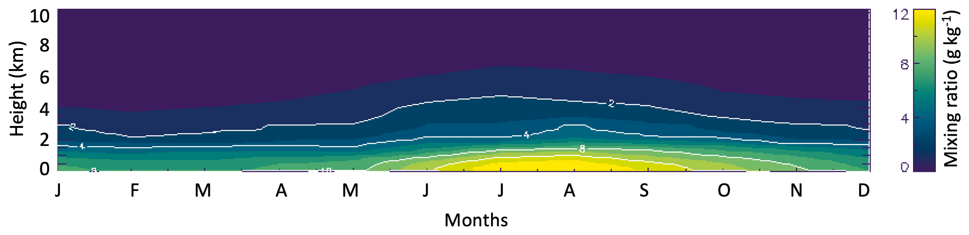
Figure 1 Monthly averaged water vapor mixing ratio (shades) and contours (white lines) from radiosondes at the ARM ENA site during marine conditions.

We utilize the mixed-layer framework that has traditionally been used to characterize the variability in boundary layer moisture and its controlling factors (e.g., Brost et al., 1982; Caldwell et al., 2005; Kalmus et al., 2014). In this framework it is assumed that the boundary layer is thermodynamically well-mixed and coupled to the surface with a constant profile of total water (vapor plus liquid) mixing ratio and liquid water potential temperature. Although previous studies have shown a prevalence of thermodynamically decoupled conditions over the open oceans (e.g., Wood and Bretherton, 2004; Serpetzoglou et al., 2008), the mixed-layer framework offers a relatively straightforward way to characterize sources and sinks of the boundary layer thermodynamic variables. In the mixed-layer framework, the boundary layer water field is modulated by advection, entrainment, precipitation, and surface latent heat flux. The validity of the mixed-layer framework has recently been shown to be sufficient to explain synoptic and monthly variability in the sub-cloud layer of the downstream trade winds near Barbados (Albright et al., 2022). However, our dataset includes a mix of coupled and decoupled cases, and it is therefore important to understand how often the assumption of a well-mixed boundary layer is verified at the site, as well as how it affects the results.

In the first part of this work, we take advantage of continuous atmospheric measurements with excellent quality available at the ARM ENA site for 5 years (2015–2020) to characterize the marine boundary layer water vapor and its controlling factors through annual mixed-layer total water budgets. In the second part we use data collected during stratocumulus cloud conditions to diagnose the relationship of the mesoscale variability in the boundary layer water vapor with cloud, precipitation, and radiation fields. Water vapor, unlike liquid water path (LWP), does not exhibit a diurnal cycle; therefore the annual and mesoscale variability are the primary modes through which the interaction between boundary layer vapor and cloud processes can be examined. Both modes influence clouds and precipitation, the annual variability being driven by large-scale advection, as shown later, and the mesoscale variability being driven by local processes.

The remainder of the paper is organized as follows: Sect. 2 presents an overview of the data and retrievals utilized with a discussion on the novelty of retrievals used to separate the contribution of cloud and drizzle to the total LWP. The annual cycle of precipitable water vapor (PWV) and LWP is discussed in Sect. 3. In Sect. 4 the validity of the mixed-layer approximation is discussed, and the marine boundary layer total moisture budget (vapor and liquid, including rain) is described in connection with the annual cycle of the vapor mixing ratio shown in Fig. 1. Finally, the mesoscale variability in water vapor during 10 selected days is analyzed in Sect. 5, and the work is concluded with a summary and discussion section.

2 Instrumentation, data, and retrievals

The Eastern North Atlantic is one of the ARM program's (Turner and Ellingson, 2016) permanent sites situated on the island of Graciosa (39.1^∘ N, 28.0^∘ W; 25 m) in the archipelago of the Azores. The climate at the site is characterized by a wide range of weather conditions influenced by the frequent arrival of midlatitude winter storms (e.g., Rémillard et al., 2012; Wood et al., 2015) and by the influence of trade winds. Recent studies have evidenced the connection between precipitation properties and large-scale conditions, for example an increased frequency of precipitating clouds in the wake of cold fronts (Lamer et al., 2020). The total cloud fraction at the site is higher in winter (Dong et al., 2014), while during summer the prevalence of a high-pressure system reduces cloud cover and promotes the prevalence of fair-weather conditions (Wood et al., 2015).

2.1 Instrumentation

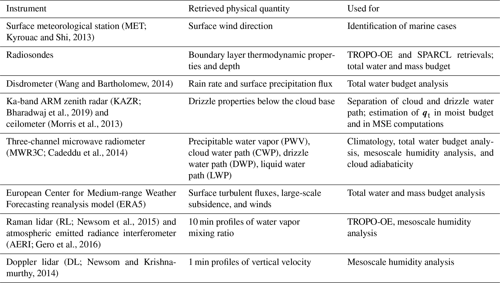
The site has several instruments to observe the aerosol, cloud, radiation, and thermodynamic fields. We mention here the main operating characteristics of the instruments used in the analysis. A vertically pointing Ka-band ARM zenith radar (KAZR) records the full Doppler spectrum and its first three moments at 2 s temporal and 30 m range resolution. The KAZR was calibrated using a corner reflector, and its accuracy is good within 3 dB (Kollias et al., 2019). A laser ceilometer operating at 905 nm wavelength records the profile of backscatter at 30 m range and 15 s temporal resolution along with the cloud-base height. A Doppler lidar (DL) operating at 1.5 µm wavelength records the backscatter and the mean Doppler velocity at 30 m range and 1 s temporal resolution. The ceilometer and the DL were calibrated by the authors using the technique proposed by O'Connor et al. (2005). The details of the technique, as applied to this site, are explained in Ghate et al. (2021). A Raman lidar (RL), collocated to the KAZR, transmits at a wavelength of 355 nm and records the backscattered radiation at wavelengths of 355, 387, and 408 nm at 10 s temporal and 7.5 m range resolution. From this instrument, profiles of water vapor mixing ratio are derived at 10 min temporal resolution. Also present at the site is a three-channel microwave radiometer (MWR3C) that measures the sky brightness temperatures at 23.8, 31.4, and 90 GHz. The MWR3C is automatically calibrated using tip curves as explained in Cadeddu et al. (2013). An atmospheric emitted radiance interferometer (AERI) measures the sky brightness temperatures from 3 to 19 µm wavelengths at 8 min time resolution. Collocated with the remote sensors is a video disdrometer that measures surface rain rates at 1 min resolution and a surface meteorological station for surface temperature, humidity, winds, and pressure at 1 min resolution. Radiosondes are launched at the site every 12 h at 00:00 and 12:00 UTC, and they measure profiles of temperature, humidity, pressure, and winds.

In addition to the instruments listed above, we also used output from the European Center for Medium Range Weather Forecasting reanalysis model (ECMWF ERA5) over the region (Rodwell and Jung, 2020). Quantities from ERA5 include hourly surface latent heat fluxes, large-scale subsidence, winds, and water vapor mixing ratio profiles. The ERA5 profiles were compared to the local soundings between 2015 and 2020 and found to underestimate the mixing ratio by about 10 % with a standard deviation of 1.0–1.6 g kg⁻¹ between 0 and 3 km and with a maximum underestimation of 15 % at the planetary boundary layer (PBL) height. The ERA5 profiles are therefore suitable for the estimation of the advection component of the budget but not suitable for the estimation of the PBL height. For this purpose, we use radiosondes. A summary of the instruments and retrievals used in the analysis is shown in Table 1.

2.2 Data selection

A total of 5 years and 4 months (1 August 2015 to 31 December 2020) of data from all instruments in Table 1 were processed, except the RL, DL, and AERI that were used only in the 10 selected cases discussed in Sect. 5. Drizzle liquid water content below the cloud base, as well as retrievals of water vapor, cloud, and drizzle water path, were derived every minute and averaged hourly to match the time resolution of the ERA5 data. After the necessary quantities were derived, cases that were classified as “only marine conditions” were identified and used for further analysis. Marine conditions were defined, following Ghate et al. (2021), by selecting data corresponding to surface wind direction (measured clockwise) greater than 310^∘ or less than 90^∘, thereby eliminating cases where the boundary layer may have been influenced by the island itself. Out of 52 608 total observations, 15 972 h (30 %) were identified as marine conditions.

Total, cloud, and drizzle water paths are produced when precipitation does not reach the surface or when it is not enough to contaminate the measurements. The mean disdrometer rain rate at the surface, when the retrievals converged, was less than 0.05 mm h⁻¹. The retrievals converged in 12 131 h (76 % of the marine cases). This limitation in the data selection due to the microwave radiometer's inability to produce reliable measurements during heavy precipitation reduces the data sample size, but it does not alter the climatological features of the dataset.

2.3 Retrievals

The KAZR and ceilometer data were combined to retrieve profiles of drizzle properties below the cloud base using the technique proposed by O'Connor et al. (2005). These retrievals were further combined with the brightness temperatures from the MWR3C to obtain water vapor, cloud, and drizzle water path using the Synergistic Passive and Active Retrieval of Cloud Properties (SPARCL) (Cadeddu et al., 2017, 2020). Uncertainties in the water vapor and LWP retrievals are estimated from the a posteriori covariance information obtained with the optimal estimation retrieval and are of the order of 0.5 mm for water vapor and about 15 g m⁻² for LWP. For 10 selected cases of weakly precipitating marine stratocumulus clouds, vertical profiles of water vapor mixing ratio were derived every 10 min using the optimal estimation retrieval TROPoe (formerly AERIoe; Turner and Löhnert, 2014; Turner and Blumberg, 2019; Turner and Löhnert, 2021). These retrievals use combined data from the RL, AERI, and microwave radiometer and have an average uncertainty of 0.6 g kg⁻¹ in the first 3 km. They are further discussed in Sect. 5.

The retrieval of LWP with SPARCL enables the separation of cloud and drizzle water path by exploiting the different signature of cloud and drizzle drops on the 90 GHz frequency of the microwave radiometer. These aspects of the retrievals are discussed in more detail in Appendix A, where a comparison with the microwave radiometer retrieval (MWRRET) is presented and the retrievals used to estimate cloud adiabaticity at the site.

Table 1 Instruments used in the analysis, physical quantities, and use of data.

3 Annual cycle

The annual cycle of water vapor and liquid water is characterized next. Consistent with Fig. 1, the PWV shows a distinct annual cycle (Fig. 2a, b) characterized by higher average water vapor in summer (2.99 cm in August) and dryer conditions in late fall and winter (1.4 cm in March). The radiometric retrievals are in good agreement with the radiosondes in both magnitude and variability. The annual cycle is mostly visible in the lower troposphere (below 3 km) but is still present, although much weaker, in the mid-troposphere above 3 km (pink boxes). The annual cycle does not have the same amplitude in the upper and lower troposphere, resulting in a stronger contribution of the free troposphere to the total PWV in summer compared to winter. The proportion of free-tropospheric PWV to the total amount ranges from 14 % in February to 20 % in June. This points towards a greater contribution of mid-tropospheric vapor towards reducing the boundary layer radiative cooling in the summer compared to the winter months.

The total LWP during marine conditions (Fig. 2c) is characterized by a weak seasonal cycle with higher LWP and higher variability during the fall and winter months. When summarized in a seasonal cycle, the mean LWP (in g m⁻²) is 82.3, 64.6, 67.3, and 75.1 g m⁻² (December–February (DJF), March–May (MAM), June–August (JJA), September–November (SON)). For these weakly precipitating clouds captured by the radiometer, the monthly mean LWP is less than 100 g m⁻² throughout the year, with maximum hourly values not exceeding 300 g m⁻². The cloud component, shown in light brown in Fig. 2c, constitutes the bulk of the total LWP (in dark brown), and it mimics the total LWP. Drizzle water path, which includes both below- and in-cloud components and is shown in Fig. 2d, is detectable through the entire year, even when the average LWP is low. Drizzle water path displays a pronounced seasonal cycle with averages in fall and winter about 17 % higher than in summer and spring. The ratio of drizzle-to-total LWP increases from ∼ 11 % in summer to ∼ 15 %–17 % in winter. This propensity of clouds with similar total LWP to produce more drizzle in winter and fall may relate to a change in the prevalent typology of clouds and to the occurrence of midlatitude winter storms in fall and winter. It points to the fact that the LWP is only one of the factors controlling drizzle production. A prominent feature of the annual cycle at the site is the weak anticorrelation between the water vapor and the LWP. This feature is discussed in more detail in the next section where the relative contribution of the processes affecting the boundary layer moisture fluxes are examined.

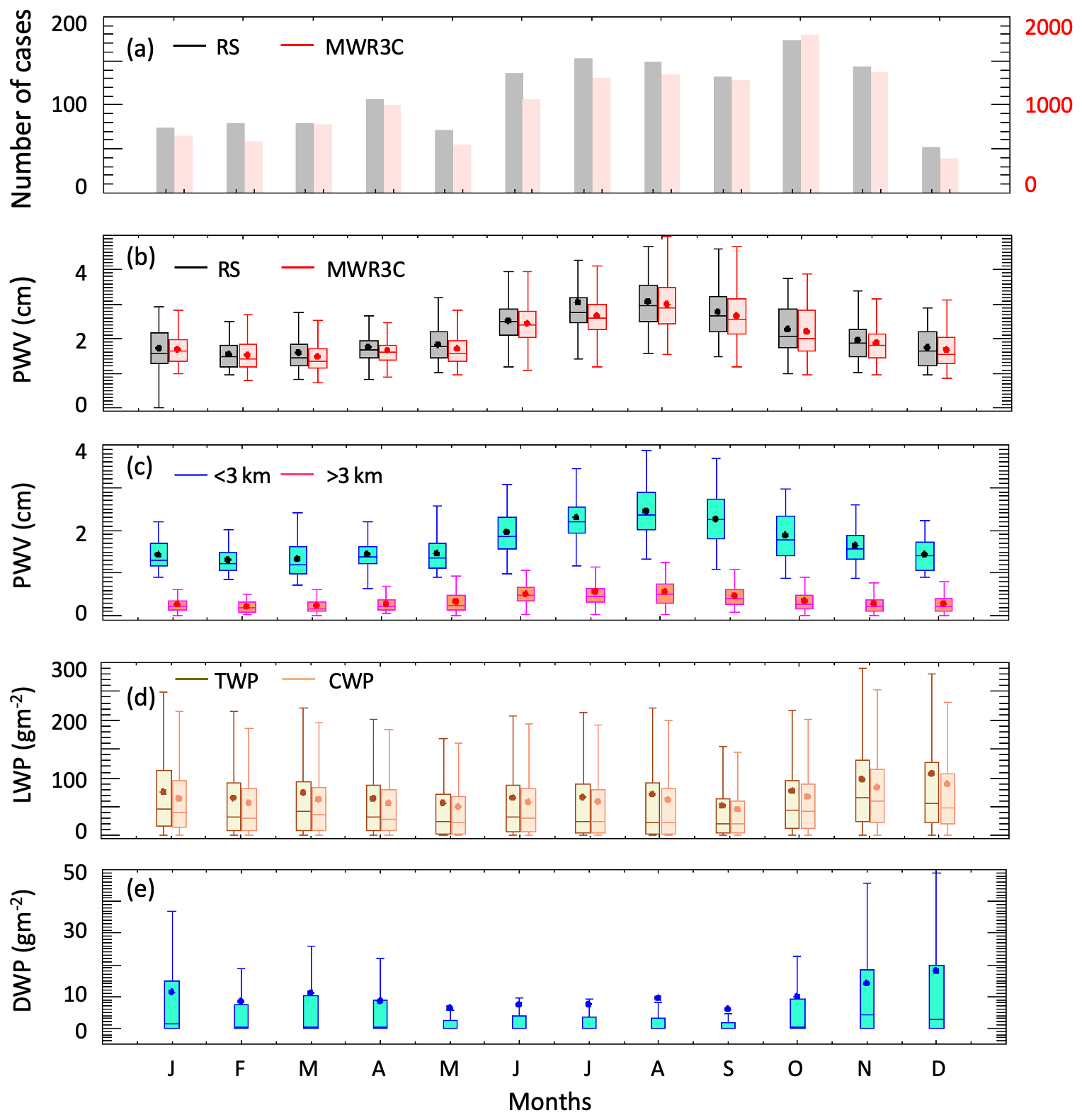
Figure 2 (a) Number of cases. (b) Annual cycle of total PWV from radiosondes (RSs) in grey and from the microwave radiometer in red. (c) Monthly mean of PWV below 3 km in cyan and above 3 km in pink from radiosondes. (d) Monthly mean total (dark brown) and cloud (light brown) water path derived from the MWR3C. (e) Monthly mean drizzle water path derived from the MWR3C. The dots denote the means, the boxes enclose the interquartile range (IQR), and whiskers extend to 1.5 times the IQR.

4 ENA site regional moisture budget

The 5 years of data, together with output from the ERA5 model, are used to estimate the boundary layer moisture budget at the ENA site. Before going into the details of the analysis we investigate the validity of the mixed-layer assumption. To this end, we examined 1825 soundings, of which 681 were marine conditions, and calculated a decoupling index (DI; Sena et al., 2016) defined as ($Z_{\mathrm{CB}}-Z_{\mathrm{LCL}})/Z_{\mathrm{CB}}$. We then classified strongly coupled cases as those with DI < 0.25 and weakly coupled cases as those with 0.25 ≤ DI < 0.4. According to this classification, most marine cases (68 %) are weakly or strongly coupled. The decoupling index is generally smaller when the cloud base is lower, and cases with cloud base <1.2 km have DI ≤ 0.4 in 80 % of the cases. A comparison between the decoupling index used in this study and the one proposed by Jones et al. (2011) is shown in Fig. S1 in the Supplement. The two indexes show that the boundary layer at the ENA site is weakly decoupled for about 60 % of the time. Examples of single profiles associated with coupled, weakly decoupled, and decoupled conditions are shown in Fig. S2.

The observations are used to investigate which large-scale processes control the moisture variability at the site on monthly and seasonal temporal scales during marine conditions. For the estimation of the moisture budget, we use the total mixing ratio ${\mathit{q}}_{\mathrm{t}}={\mathit{q}}_{\mathrm{v}}+{\mathit{q}}_{\mathrm{l}}$, which is the sum of water vapor mixing ratio (q_v) and liquid mixing ratio (q_l), including rain, when clouds are present and follow the formulation of Caldwell et al. (2005). We therefore express the boundary-layer-averaged formulation as follows (in units of W m⁻²):

$$\begin{array}{}\text{(1)}& {\displaystyle \frac{L}{g}}\widehat{p}\left({\displaystyle \frac{\partial \langle {\mathit{q}}_{\mathrm{t}}\rangle }{\partial t}}+\langle \mathit{v}\cdot \mathrm{\nabla }{\mathit{q}}_{\mathrm{t}}\rangle \right)-\mathrm{LHF}-LP-{\displaystyle \frac{L}{g}}{\widehat{\mathit{\omega }}}_{\mathrm{e}}\mathrm{\Delta }{q}_{\mathrm{t}}=\mathrm{0},\end{array}$$

where L and g are the latent heat of vaporization (2.5×10⁶ J kg⁻¹) and the acceleration due to gravity (9.8 m s⁻²), 〈x〉 indicates averages between the surface and the top of the boundary layer, and $\widehat{p}=p_{\mathrm{0}}-p_{\mathrm{t}}$ is the difference between surface pressure and pressure at the top of the boundary layer. The first two terms represent the time change in the PBL-averaged moisture (local tendency) and the large-scale horizontal advection to the region with v being the wind vectors and ∇q_t the horizontal gradient. The third and fourth terms represent the surface latent heat fluxes (LHFs) as reported by ERA5 and the precipitation fluxes obtained from the disdrometer rain rate (P; expressed in kg m⁻² s⁻¹) and multiplied by the latent heat of vaporization (L). The last term in Eq. (1) is related to the turbulent fluxes due to entrainment of dry air at the top of the boundary layer. Specifically, ${\widehat{\mathit{\omega }}}_{\mathrm{e}}$ is the entrainment velocity and Δq_t the gradient of the total water mixing ratio across the top of the boundary layer. Some quantities necessary in Eq. (1) are not available from measurements and are therefore calculated using ERA5 reanalysis data as shown in Table 1. Below we provide an overview of the data and details on the methodology used to calculate each term. All the terms were estimated on an hourly basis and averaged each month. All components were screened for outliers eliminating points beyond 2 standard deviations from the monthly mean and were passed through a 24 h running average. The vertically gridded data (radiosondes and ERA5 profiles) were interpolated on a common vertical grid of 50 m vertical resolution. Values for the quantities in Eq. (1) are shown in units of watts per square meter (W m⁻²) in all the subsequent analysis.

4.1 Datasets used for each term

The PBL height is used to determine the highest limit for integrating the water vapor profiles and to calculate the entrainment rate. The ARM value added product (VAP) available from the ARM archive (Sivaraman et al., 2013) reports PBL heights from the radiosondes based on the Heffter (1980) method that identifies the base of the inversion from the gradient of the potential temperature. Because the ENA site only launches two radiosondes per day (at 00:00 and 12:00 UTC), we assume the PBL height to be as reported by the radiosonde within ±6 h of each radiosonde. If PBL height data were not available for 1 entire day, the day was flagged as missing. Uncertainty in the estimation of PBL height from radiosondes is estimated to be 100–200 m (Sivaraman et al., 2013). This is a lower-limit estimate in our case because the PBL height is kept constant for 12 h.

The local change $\frac{\partial \langle {\mathit{q}}_{\mathrm{t}}\rangle }{\partial t}$ in the moisture profile at the site was estimated as follows: vertical profiles of q_v are available from radiosondes twice a day. The vertical distribution of humidity between 00:00–12:00 UTC (12:00–24:00 UTC) was kept constant and equal to the morning (evening) radiosonde reported values. The profiles were scaled to the MWR3C-retrieved hourly PWV using a height-independent scale factor (e.g., Turner et al., 2003). For the estimation of q_l, the hourly averaged cloud LWP from the SPARCL retrieval was distributed adiabatically between cloud base and cloud top. Because the PBL height is only available twice per day or less, monthly profiles of PBL heights were used to identify the top of the boundary layer. The errors introduced by this approximation are small because of the limited variability in the PBL height, as shown later. Profiles of ${\mathit{q}}_{\mathrm{t}}={\mathit{q}}_{\mathrm{v}}+{\mathit{q}}_{\mathrm{l}}$ were then averaged between the surface and the top of the boundary layer, and the difference between successive hours was calculated and multiplied by $\widehat{p}$. The uncertainty of this term is driven by the uncertainty of the microwave radiometer retrievals that is estimated as 0.5 mm for water vapor and 15 g m⁻² for the LWP. This translates into an uncertainty of less than 0.25 g kg⁻¹ for the average q_t.

The large-scale moisture advection 〈v⋅∇q_t〉 was estimated from ERA5 data by calculating the horizontal gradient of the moisture field across grid points adjacent to the ENA site using the following equation:

$$\begin{array}{}\text{(2)}& \mathit{v}\cdot \mathbf{\nabla }{q}_{\mathrm{t}}={\mathit{v}}_{\mathrm{NS}}{\displaystyle \frac{\partial {\mathit{q}}_{\mathrm{NS}}}{\partial {\mathit{x}}_{\mathrm{NS}}}}+{\mathit{u}}_{\mathrm{EW}}{\displaystyle \frac{\partial {\mathit{q}}_{\mathrm{EW}}}{\partial {\mathit{x}}_{\mathrm{EW}}}},\end{array}$$

where v_NS and u_EW are the boundary-layer-averaged meridional and zonal components of the wind, and gradients denote differences – ${\mathit{q}}_{XY}={\mathit{q}}_Y-{\mathit{q}}_X$ – between grid points (0.25 × 0.25^∘) adjacent to the ENA site. The bold notation indicates that the differences are calculated at all vertical points before averaging over the boundary layer. Note that only the vapor component was estimated, and the contribution of liquid water advection was neglected. As we selected only marine conditions for our analysis, we expect this component to be dominated by a prevalence of colder and drier air from the north. The uncertainty of the advection term is hard to estimate. From a comparison of ERA5 and radiosondes profiles at the ENA site the mixing ratio uncertainty is expected to be around 10 % with higher uncertainty of 15 % near the top of the boundary layer, where the humidity gradient is located. Hourly values of surface latent heat flux from the ERA5 reanalysis model data are used for this analysis. Precipitation data from the disdrometer at the site were hourly averaged and passed through a 24 h running average to eliminate excessive noise. The last term of the budget in Eq. (1) requires the evaluation of the moisture gradient at the top of the boundary layer and of the entrainment rate (see Sect. 4.2). The term Δq_t was defined as the difference between the total mixing ratio above the boundary layer inversion and the PBL-averaged q_t and was therefore estimated from radiosondes, retrieved water vapor, and cloud LWP. The largest uncertainty in this term is the PBL height that is estimated to be 100–200 m. The annual cycle of all the quantities described above is shown in Fig. 3.

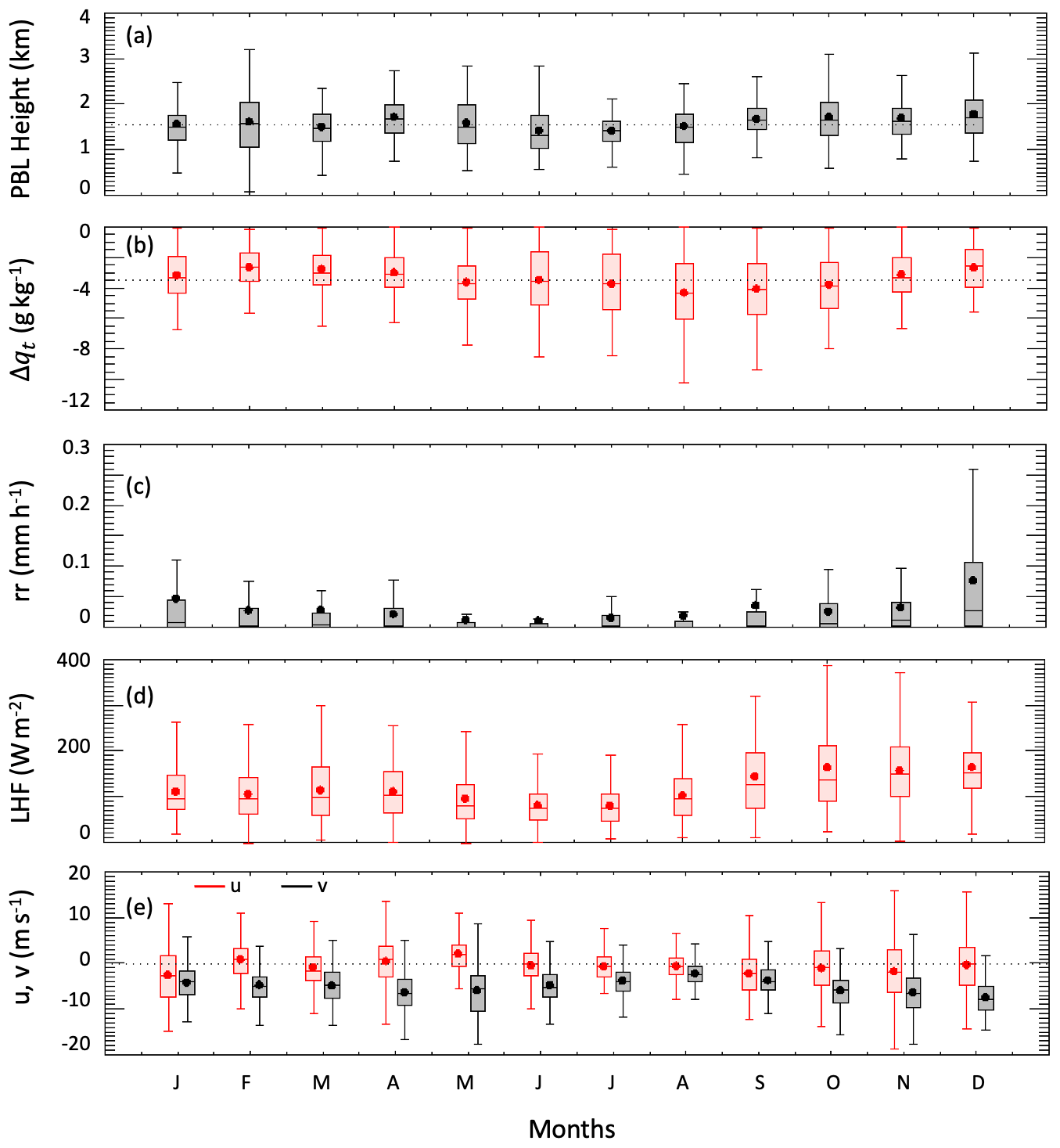
Figure 3 Monthly box and whisker values of (a) PBL height, (b) humidity gradient at the boundary layer top, (c) rain rate, (d) latent heat fluxes, and (e) zonal (u) and meridional (v) components of the wind. Dotted lines represent the annual mean in (a) and (b) and the zero line in (e).

The monthly mean PBL height did not display a marked annual cycle but rather small perturbations around an annual mean value of 1.6±0.5 km. On average a deeper boundary layer (1.7 km) is found in fall, and a shallower boundary layer (1.4 km) is found in June and July. During summer months, the humidity gradient at the PBL top was strongest and exhibited the greatest variability. Conversely, a deeper average boundary layer in fall and winter had weaker humidity gradients at the PBL top. The southward boundary layer winds were stronger in the winter months compared to the summer months and so were the surface LHF fields and rain rates. Collectively, this figure suggests that winter months exhibit on average a deeper boundary layer, weaker boundary layer inversion, and higher winds, fluxes, and rain rates compared to the summer months. This is consistent with the finding in Ghate et al. (2021), who observed higher boundary layer turbulence in winter than in summer.

4.2 Boundary layer mass budget and entrainment rates

Assuming a near-constant air density within the boundary layer, the mass budget can be written in terms of the changes in PBL height. Here we utilize the boundary layer mass budget to calculate the entrainment rates on monthly timescales. The entrainment velocity at the boundary layer top is balanced by local changes in the boundary layer height, advection of the PBL top, and large-scale vertical air motion at the PBL top (Eq. 3).

$$\begin{array}{}\text{(3)}& {\mathit{\omega }}_{\mathrm{e}}={\displaystyle \frac{\partial \widehat{p}}{\partial t}}+\mathit{v}\cdot \mathbf{\nabla }\widehat{p}-{\widehat{\mathit{\omega }}}_{\mathrm{s}}\end{array}$$

Following Wood and Bretherton (2004), all terms were averaged monthly before being used in Eq. (3), and the monthly averages of the terms were additionally filtered to eliminate outliers beyond 2 standard deviations from the mean and unphysical values and to reduce the large noise of the dataset. The term $\frac{\partial \widehat{p}}{\partial t}$ was computed taking the difference between two successive soundings (12 h time step). Advection of the PBL top $\mathit{v}\cdot \mathbf{\nabla }\widehat{p}$ and the large-scale vertical air motion were estimated from ERA5. Although the mass budget was computed in pressure units (Pa s⁻¹) for the calculations of the fluxes in Eq. (1), we convert it to millimeters per second (mm s⁻¹) for the figures and in the following discussion to facilitate comparison with previous work.

The monthly mean components of the mass budget and resulting entrainment rates are reported in Table S1 in the Supplement. The annual mean local tendency of the PBL top, advection, and large-scale subsidence at PBL top were −0.0061, 0.012, and 0.036 Pa s⁻¹, which translate approximately into 0.6, −1.0, and −3.2 mm s⁻¹ respectively. The values of the local tendency of the PBL top and advection were small during all months, and the advection of the boundary layer height was less than 40 % of the entrainment rate in winter but was somewhat more prominent in summer. The small contributions of the local tendency and of the advection term resulted in a near balance between entrainment velocity and subsidence (Fig. 4). Entrainment rates exceeded subsidence of ∼ 20 % in January, and for the rest of the months entrainment was balanced or was slightly weaker than subsidence. However, the high standard deviation indicates a large variability throughout the year. The near balance of entrainment and large-scale subsidence is consistent with the observed small variability in the PBL height. On average, the entrainment rates found here are slightly lower than what was reported in Wood and Bretherton (2004) along the Pacific coast; the variability is, however, well in the range of values found in previous studies. The calculated entrainment rates (ω_e) display a weak annual cycle with higher values in fall and winter and lower values in summer, with averages varying from 1.7 mm s⁻¹ in July to 4.1 mm s⁻¹ in January. The annual cycle is consistent with higher turbulence during the winter months compared to the summer months. These values are also in broad agreement with those found in previous studies at different locations (e.g., Painemal et al., 2017; Ghate and Cadeddu, 2019; Albrecht et al., 2016) for stratocumulus clouds.

Figure 4 Monthly entrainment rates ω_e and subsidence rates ω_s with associated 1 standard deviation.

4.3 Monthly and seasonal moisture budget

With all the terms in Eq. (1) accounted for, the annual cycle of the moisture budget is shown in Fig. 5. Because the focus is on marine conditions, the large-scale advection is predominantly from the north and hence represents a boundary layer drying along with entrainment and precipitation. The local tendency term is often assumed to be zero (e.g., Caldwell et al., 2005; Kalmus et al., 2014) but here is calculated explicitly for each month. The term is small and, except for the months of January and May, acted as a weak moisture sink. Annually, the surface latent heat flux, which constitutes the only moisture source, is balanced by the local change, advection, entrainment, and precipitation with a residual term of −1.4 W m⁻². The fluxes are highest in the winter months and lowest in the summer months, anti-correlated to the boundary layer vapor annual cycle shown in Figs. 1 and 2a and b. This largely represents the meteorological correlation of calmer winds, lower sea-air temperature difference, shallower boundary layers, and weaker advection with increased vapor loading during the summer months compared to the winter months. At this point we are in the condition to evaluate the impact of including decoupled conditions in the analysis. We repeated the budget computations including only a subset with cloud base <1.2 km, which presents mostly coupled conditions. The results showed a diminished contribution of the entrainment fluxes that decreased annually from 26 % to 18 %. It is therefore likely that the inclusion of decoupled conditions in the analysis leads to an overestimation of the moisture sink due to entrainment fluxes.

The large-scale advection term is the largest moisture sink. The contribution from advection in October and December is almost twice the contribution in June and July. Corresponding to the advection of colder and dry air from the north, latent heat fluxes increase from September to December. In November and December, the monthly vapor source and sink budget are not entirely balanced with higher residuals in November and December. To better summarize the dataset, Fig. 5b and Table 2 show the seasonal values of all terms and the residuals. Seasonally the positive (LHF) and negative terms of the moisture budget balance to within ±20 W m⁻². As shown in Table 2 there are large standard deviations associated with the single components of the budget. These standard deviations are partially a result of the uncertainty associated with the computations of the terms (model, measurements, retrievals, approximations, etc.) and are also due to the broad range of atmospheric conditions encountered in the dataset used. The budget closure is well within the estimated uncertainty. Averaged annually, the moistening from the surface is primarily balanced by advection drying (∼ 50 %) and entrainment drying (∼ 25 %) with the rest compensated through precipitation removal. Overall, the budget analysis highlights the complexity of the moisture variability in the region as advection is determined by large-scale features external to the boundary layer, while the entrainment and precipitation are determined by boundary layer internal properties. This point is discussed further in the last section.

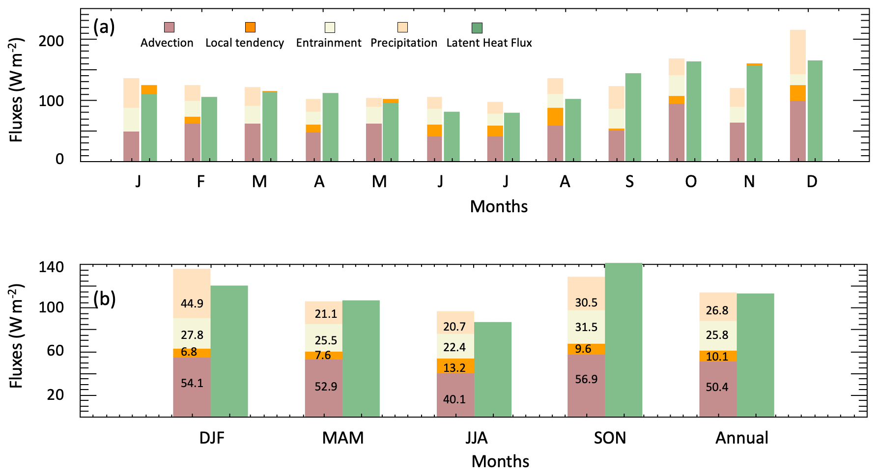
Figure 5 Monthly (a) and seasonal (b) components of the moisture budget. The left bars are moisture sinks, and the right bars are moisture sources. Color bars represent advection (brown), local tendency (orange), entrainment (cream), precipitation (pink), and latent heat fluxes (green). Numbers in the bottom plot are percent values. The residual terms are not shown in this figure.

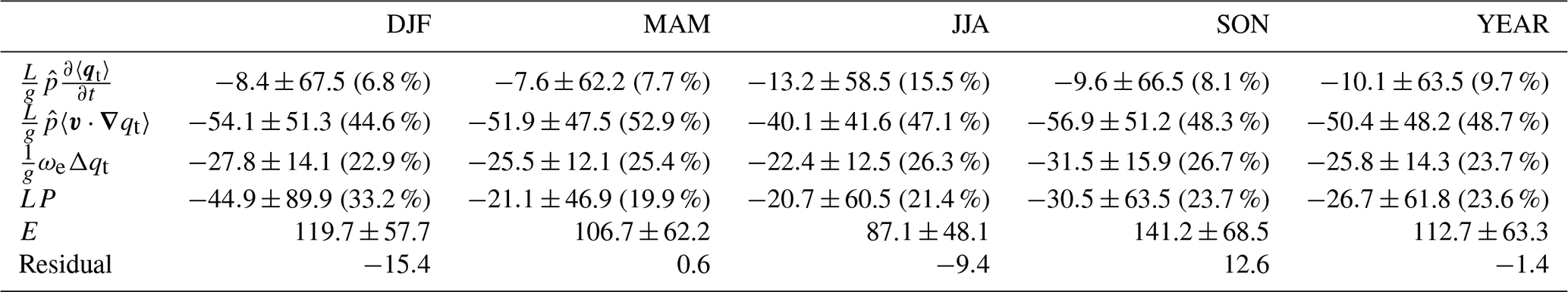
Table 2 Seasonal average values and standard deviation of the budget components. In parenthesis are the contributions of each negative term to the total boundary layer drying. Residuals are computed as the difference between source and sinks (W m⁻²).

5 Mesoscale variability in water vapor

Besides the annual variability, water vapor also presents a mesoscale variability that is strongly connected to clouds and precipitation. Therefore we now focus on shorter timescales (days and hours) to understand how mesoscale perturbations of water vapor locally affect boundary layer radiative cooling, clouds, turbulence, and precipitation. Mesoscale organizations of clouds are visible from satellites and have been extensively studied to understand how they affect or are affected by water vapor and precipitation (Stevens et al., 2020; Wood and Hartmann, 2006; Bretherton and Blossey, 2017). Mesoscale self-aggregation is not, however, easily discernible with ground-based observations, and some attempts have been made at gathering observational evidence from satellites (Lebsock et al., 2017) and from specific sites and reanalysis (Schulz and Stevens, 2018). Here we focus on the spatial organization of water vapor on a scale of 10 km by identifying its perturbations over a background state, similarly to the framework recently developed by Zhou and Bretherton (2019).

5.1 Hourly spatial and temporal distribution of moisture

To analyze the mesoscale (10 km) distribution of water vapor, we use 1 min averaged PWV and LWP from the radiometer and rain rate from the disdrometer during 10 selected days at the ENA site between 2016 and 2019. A list of selected cases is in Table S2 in the Supplement. The selected days displayed persistent boundary layer cloudiness and at times precipitation. We also use vertical profiles of mixing ratio below the cloud base from the combined RL, AERI, and two-channel microwave radiometer (MWR) observations (see TROPO-OE in Table 1) produced every 10 min and then linearly interpolated over 1 min. When compared to radiosondes at the site, the coincident TROPO-OE retrievals reproduce the mean profile well. The bias between radiosondes and retrievals is less than 0.35 g kg⁻¹ (or less than 6 %) from 150 m to the cloud base, and the standard deviation of the differences is about 0.1 g kg⁻¹ (Fig. S3). Hence the retrieved vertical profiles of mixing ratio are well suited to investigate the mesoscale variability in the moisture field.

The background water vapor value is found by implementing a running average window with a width of 100 km on the PWV, and a (sub-mesoscale) perturbed field is found by implementing a running average window with a width of 10 km. Because the data are on a uniform 1 min time grid (= 60 s), the number of minutes over which the averages are performed is determined through the daily average wind speed at cloud base as derived from the interpolated sondes at the site. For example, if the average wind speed is 7 m s⁻¹, the full mesoscale window is obtained by averaging over 24 min. The background field is subtracted from the perturbed field to identify the magnitude of the mesoscale perturbations. Mesoscale regions with positive differences are “moist” cells, and those with negative differences are “dry” cells. The statistics of the 345 identified perturbations are shown in Fig. 6.

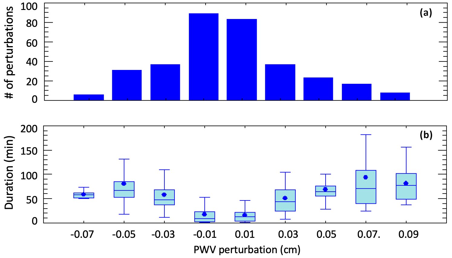
Figure 6 (a) Distribution of the 345 water vapor perturbations found in the 10 d analyzed. (b) Duration of water vapor perturbations binned by the amplitude of the perturbation: N = 6, 31, 37, 89, 83, 37, 23, 17, and 8 for a total of 331 points. The 14 missing cases are distributed in the bins below −0.07 cm and above 0.09 cm with fewer than five points in each bin. A duration of ∼ 30 min corresponds to a wind speed of 5 m s⁻¹, and a duration of 50 min corresponds to a wind speed of ∼ 3 m s⁻¹.

About half (57 %) of the mesoscale perturbations are weak and of short duration (∼ 25 min), 37 % of the perturbations are of medium magnitude (±0.05 cm), and about 6 % of them can be classified as strong (±0.1 cm). Positive and negative perturbations balance each other in strength with a slight prevalence of positive perturbations for the strongest cases as shown later. The duration of the perturbations is proportional to their strength. Medium and strong perturbations last on average 68 and 129 min (1.1 and 2.15 h) respectively indicating a marked difference in the wind speed at the cloud base.

Examples of a case with strong and weak mesoscale organization are shown in Fig. 7. The day of 4 April 2019 was characterized by intermittent precipitation and areas of higher localized moisture in regions of precipitating shafts. The vertical distribution of the mixing ratio perturbations from the background state clearly shows a spatial structure where columns of moist and dry cells alternate over the site. Moist regions are located below the cloud base and inside the precipitating shafts. The moist columns correspond to regions of increased LWP and precipitation. In the absence of precipitation (as for example towards the end of 8 June 2019) mesoscale perturbations from the background state are absent, and the spatial structure of the mixing ratio perturbations is less defined.

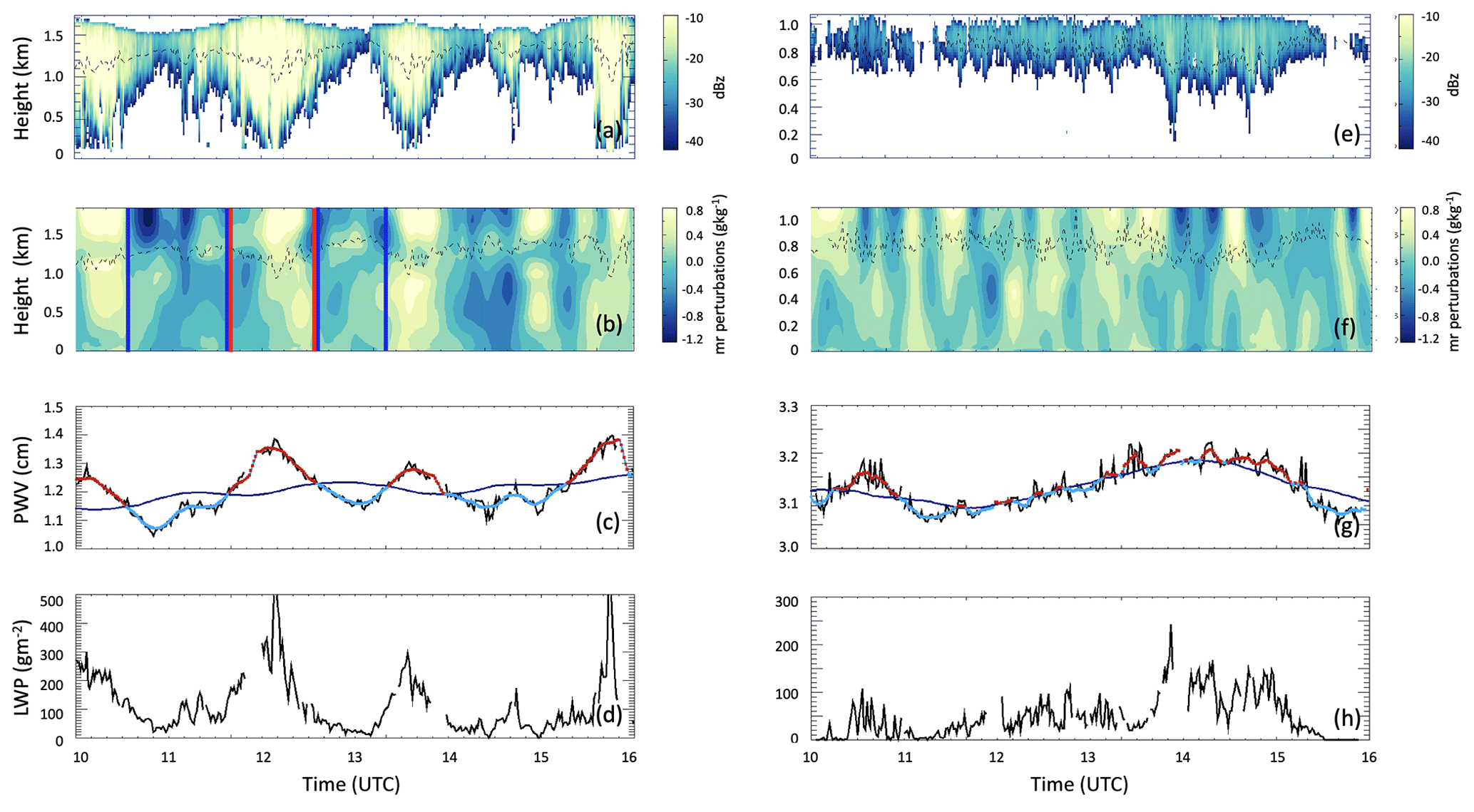
Figure 7 From the top: radar backscatter, mixing ratio (mr) perturbations, PWV, and LWP on 4 April 2019 (a–d) and 8 June 2019 (e–h). The blue and red vertical bars in (b) represent examples of the beginning and the end of dry (blue) and moist (red) adjacent columns. The dark blue line in (c) is the background state, and red and cyan segments mark moist and dry perturbations.

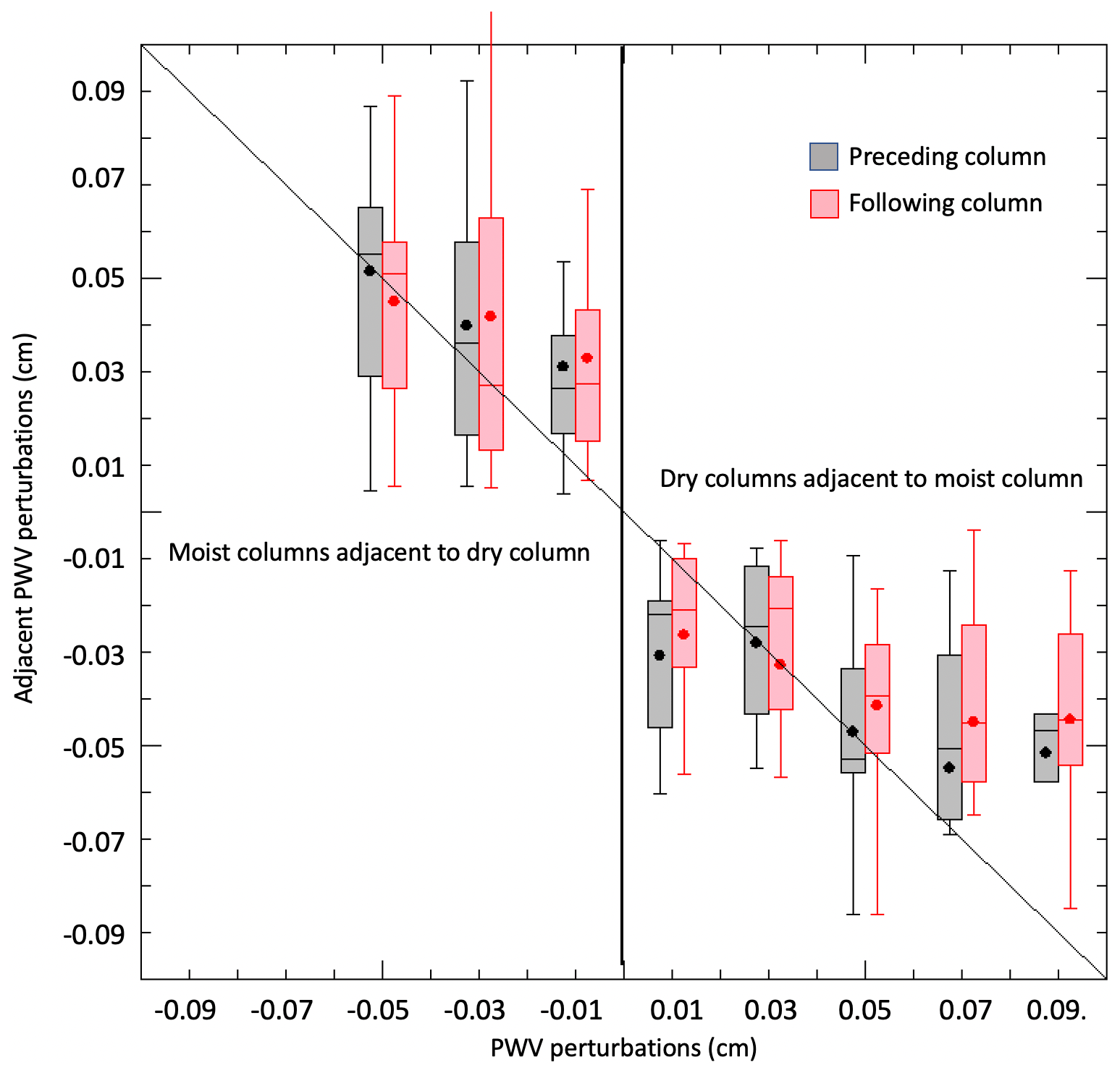
Figure 8 Average water vapor perturbations in the columns preceding (black) and following (red) a central perturbation identified on the x axis. The diagonal line indicates the point where vapor perturbations in adjacent columns have the same magnitude as the central column: N = 25, 22, 19, 15, 20, 15,13, and 5 for a total of 134 points. The nine missing cases are distributed in the bins below −0.05 cm and above 0.09 cm with fewer than five points in each bin.

Moist and dry neighboring columns lasting longer than 10 min for a total of 143 columns were identified, and the average properties of each cell were compared to those of its preceding and following neighbors. The turbulence forcing (cloud-top cooling, surface fluxes, etc.) varied greatly between the cases, and hence we chose to characterize the differences between neighboring columns rather than aggregate them solely based on the water vapor perturbations as was done in Zhou and Bretherton (2019). Our results are, however, consistent with theirs.

Figure 8 shows that dry and moist columns are preceded and followed by perturbations of the opposite sign and similar amplitude. The exception are cases in which there are strong positive perturbations represented by the last two bins on the right (PWV perturbations >0.05 cm). In this case the dry neighbors on each side of the moist cell are weaker and present a weak asymmetry between the preceding and the following dry columns, with the preceding column being somewhat drier than the following column.

The few cases in the last bin are not sufficient to provide a valid sample from which to draw definite conclusions. We calculated cloud-top radiative cooling, rain rate, cloud, and drizzle water path in each dry and moist mesoscale column. These are shown in Fig. 9 as differences between the central and the two adjacent columns. Moist patches always have stronger (more negative) cloud-top cooling compared to the adjacent dry regions, even when the water vapor perturbation is weak, but a dependence on the magnitude of the vapor perturbation is only visible in the last three bins where average differences as high as −60 W m⁻² can be reached. Similarly, there are substantial differences between adjacent dry and moist cells in cloud water path, drizzle water path, and rain rate.

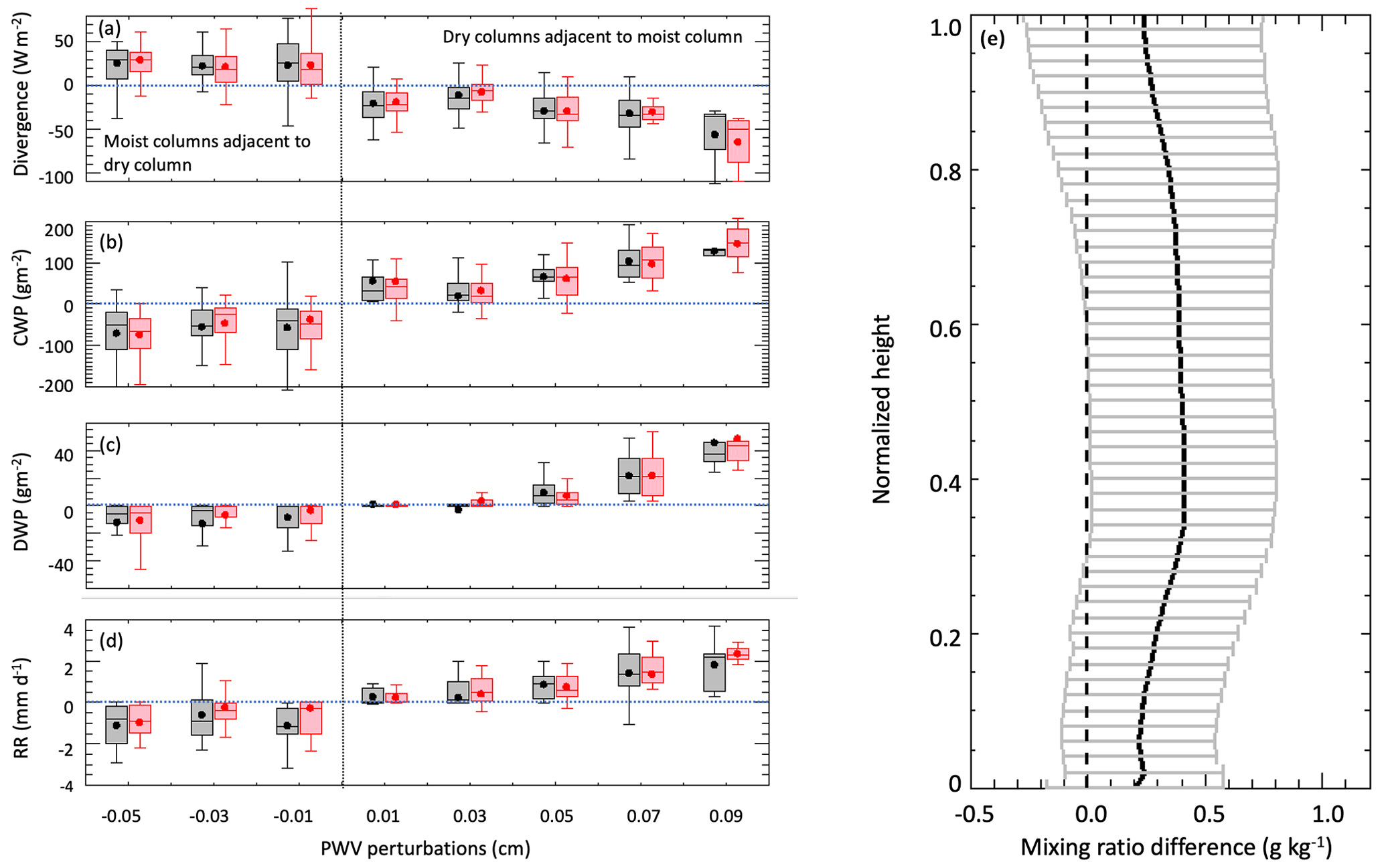
Figure 9 (a–d) Differences in cloud-top radiative cooling, cloud water path, drizzle water path, and rain rate at cloud base between each identified region (x axis) and the two adjacent regions binned by the strength of the region's PWV perturbation: N = 25, 22, 19, 15, 20, 15, 13, and 5. Differences are computed as center-minus-preceding (black) and center-minus-following (red) columns. (e) Vertical distribution of the mixing ratio differences between moist and dry columns. The height is normalized to the cloud-base height.

Moist cells always have a higher LWP and precipitation. Small differences in drizzle water path and rain rate between positive and negative columns are still noticeable in the presence of weak vapor perturbations (< 0.03 cm). This weak drizzle associated with a modest increase in the LWP may be driven by the stronger radiative cooling (∼ 25 W m⁻²) in the positive columns. In the presence of strong (>0.03 cm) positive vapor perturbations, differences between moist and dry columns increase proportionally to the vapor perturbations indicating some correlation between the amount of moisture in the boundary layer and the amount of drizzle and rain rate in the mesoscale column. Mixing ratio differences between moist and dry columns are not uniformly distributed but are instead higher in the middle of the boundary layer as shown by the average vertical distribution in Fig. 9.

5.2 Vertical air motion and moist static energy

Among the mechanisms proposed for mesoscale aggregation, shallow convection is one in which vertical air motion promotes moisture transfer from the dry to the moist columns, thereby increasing moisture variance (Bretherton and Blossey, 2017; Geet et al., 2022). In the theoretical framework, a mesoscale circulation is characterized by updrafts in the moist columns and subsiding dry air in the dry columns. With the help of the DL we therefore examine the vertical velocities in moist and dry cells and compare them among adjacent regions in the sub-cloud layer. Only heights where at least 80 % of the DL readings are valid in a layer are used in calculating these averages. This resulted in a total number of updrafts between 10³ and 10⁴ in the lower half of the boundary layer and between 10² and 10³ in the sub-cloud level. The samples were averaged inside each of the 143 moist and dry columns. Figure 10 points to increased updraft frequency in the moist columns and increased downdraft frequency in the dry columns immediately below the cloud base. In the same vertical range, downdrafts are slightly stronger in dry columns (10 %–15 %) but not in a statistically significant way. Similarly, in the sub-cloud layer (Fig. 10c) the variance of vertical velocity is 20 %–60 % higher in the dry columns than in the moist columns. Looking at the relative contribution of updrafts and downdrafts in moist and dry columns, Fig. 10d shows that updrafts in moist and dry columns contribute to the total variance mostly in the bottom part of the boundary layer. In the dry columns the contribution of downdrafts increases from 40 % near the surface to 60 % below the cloud base. Although the shown differences are not statistically significant due to limited samples, these observations point towards the existence of a subsidence region of increased turbulence in the sub-cloud layer of the dry patches where dry air may be entrained and eventually mixed in the boundary layer, eventually reinforcing the drying. On the other end there may be a reinforcing of the moistening in the moist columns through the lower troposphere and the lifting up of moist air in the sub-cloud layer. To examine this part, we show in Fig. 11 curves of moist static energy (MSE) and virtual liquid static energy for the moist columns and adjacent dry columns in the 2 d shown in Fig. 7. The MSE in moist and dry columns is similar between the surface and the lower boundary layer. As previously mentioned, in a well-mixed boundary layer, conserved quantities such as the liquid water potential temperature are constant, and the moist static energy is also conserved. Dry columns have a similar MSE compared to moist columns near the surface but a lower MSE in the upper part of the boundary layer, starting in the layers immediately below the cloud base. This appears to confirm the concave nature of the MSE and virtual liquid static energy relationship shown by the previous modeling study of Bretherton and Blossey (2017).

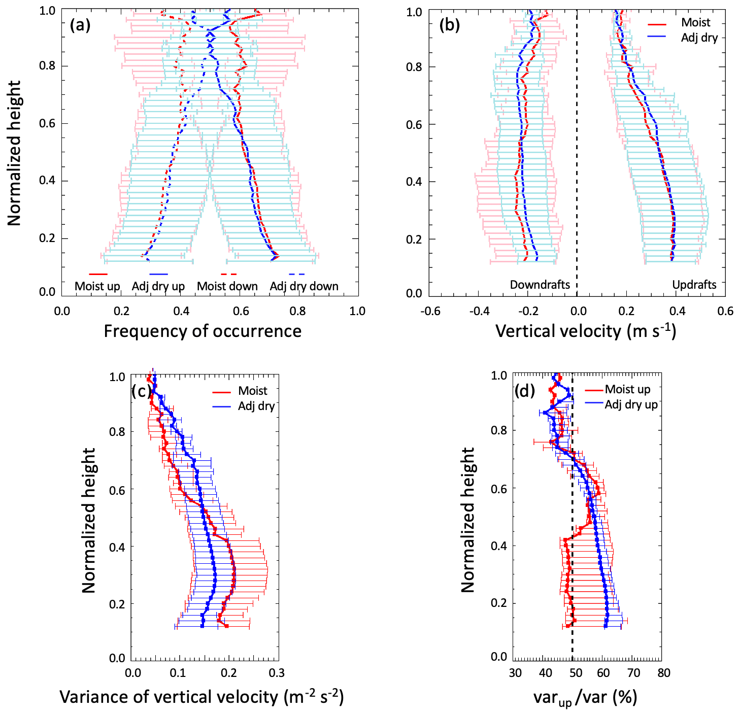
Figure 10 (a) Frequency of updrafts and downdrafts, (b) vertical velocity, (c) variance of vertical velocity in moist (red) and adjacent dry (blue) columns, and (d) contribution of updrafts to total variance in moist and dry columns. The contribution of downdrafts can be estimated as 100 − 100 ⋅ ${\mathrm{var}}_{\mathrm{up}}/\mathrm{var}$. The height is normalized to the cloud-base height.

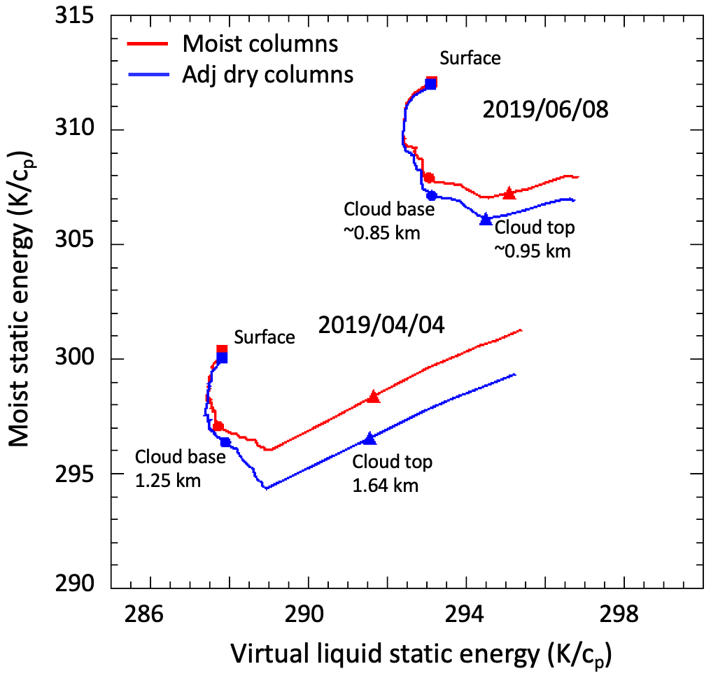
Figure 11 Average moist static energy versus virtual liquid static energy in moist and adjacent dry columns of the 2 d shown in Fig. 9. Squares, circles, and triangles indicate surface, cloud base, and cloud top.

6 Discussion and conclusions

In this work we have examined the factors that control marine boundary layer moisture at the ARM ENA site on a seasonal and daily temporal scale using 5 years of ground-based observations and reanalysis data. Unlike LWP, water vapor at the site does not present a diurnal cycle but presents an annual and mesoscale variability that is strongly connected with cloud and precipitation at the site. To our knowledge, the present analysis is also the first study to characterize and determine the controls of moisture variability at a subtropical marine location, such as the ENA site, using a long-term dataset of ground-based data. The boundary layer water vapor was highest during the summer months and lowest during the winter months. The mid-tropospheric humidity was also highest during the summer months and lowest during the winter months. The annual cycle of boundary layer (BL) water vapor is anti-correlated to the annual cycle of cloud and drizzle water path, highlighting the complex interaction between water vapor and clouds in the region. During winter months, turbulence, rather than water vapor, appears to be the primary controlling factor of cloudiness in the region (Ghate et al., 2021). An analysis of cloud adiabaticity shown in Appendix A also shows that clouds are slightly more adiabatic in winter. This could be associated with deeper boundary layers, stronger turbulence, and a higher prevalence of thermodynamically coupled boundary layers during the winter months as compared to the summer months (Wang et al., 2022).

Monthly marine boundary layer water budgets were estimated using the mixed-layer framework. Although the majority of marine cases at the site can be classified as coupled or weakly coupled, the inclusion of decoupled cases in the analysis introduces uncertainties leading to an overestimation of the contribution of entrainment fluxes to the budget. The analysis shows that moistening from the latent heat flux is balanced mostly by the large-scale advection of colder and drier air (∼ 50 %), followed by entrainment drying (20 %) and precipitation removal (∼ 15 %). Latent heat fluxes are enhanced in fall and winter, resulting in average fluxes that are 26 % stronger in winter and 22 % weaker in summer compared to the annual mean. Although significant effort was spent in producing high-quality retrievals with low uncertainty bounds (Cadeddu et al., 2020), the moisture budgets could not be fully closed with an annual residual term of ∼ 9 W m⁻² and larger monthly residuals. This primarily stems from the lack of PBL height and BL inversion strength observations at hourly timescales, as they are derived from the radiosonde launches made every 12 h. Additional uncertainty is introduced due to the direct measurement of BL entrainment rates that are derived from the mass budget and necessitate reanalysis-predicted PBL depth. Measurements of surface and BL thermodynamic properties around the site, such as those available at the ARM Southern Great Plains (SGP) site, can possibly alleviate this issue.

On a daily temporal scale, we examined the mesoscale (10–100 km) organization of water vapor for 10 d, characterized by stratocumulus cloud conditions. Differences in water vapor mixing ratio, LWP, rain rate, cloud-top radiative cooling, moist static energy, and vertical air motion between adjacent moist and dry mesoscale columns of vapor passing over the site were calculated. In these mostly drizzling systems, there are sharp differences between moist and dry patches, with moist cells always displaying stronger cloud-top cooling and higher LWP and precipitation. Differences between moist and dry patches increase when the vapor perturbations are stronger, suggesting some control of water vapor over the amount of precipitation; however, even in the presence of weak moist perturbations, there are detectable differences in precipitation and LWP suggesting a role of turbulence in drizzle initiation. Moist and dry patches present differences in vertical velocity with dry regions (dashed blue lines in Fig. 10a) displaying more frequent downdrafts than moist regions (dashed red lines) immediately below the cloud base. In the same layers, downdrafts in the dry columns appear 10 %–15 % stronger and the variance of vertical velocity 10 %–28 % higher. Finally, profiles of moist static energy in adjacent moist and dry columns show a similar MSE in the lower boundary layer, decreasing in the dry cells near the cloud base. Additionally, the departure of MSE versus liquid static energy from a straight line implies a difference in the vertical mixing between moist and dry columns, conditions that would be favorable to the maintenance and amplification of the moisture variance and the mesoscale organization. These results suggest the presence of mesoscale convective aggregation in marine low clouds, as hypothesized in the previously cited works, which is not represented in current ESMs that have spatial resolutions of 100 km or greater. However, as the ESMs increase in spatial resolution (e.g., Caldwell et al., 2021), the cloud parameterizations will have to account for the small-scale processes that cause this mesoscale aggregation.

As a final consideration we would like to spend a few words to highlight how the separation of cloud and drizzle water path in the new retrievals reveals the ubiquitous presence of drizzle throughout the year even in seasons when the average LWP is low. By looking only at the total LWP, only a weak annual variation appears; however, the drizzle LWP shows a more pronounced seasonal variability, pointing to the fact that LWP is only one of the factors influencing drizzle formation. These results can be useful for future observational studies aimed at understanding the combined effects of aerosols and turbulence in the development of precipitation, pointing to the importance of looking at processes seasonally. With the presence of mesoscale cellularity and with turbulence being higher in the winter as compared to the summer, we expect the aerosol effects on the low clouds to be more dominant in the summer months compared to the winter months. In addition, the characterization of changes in cloud and rain properties due to aerosols will also need to involve the proper characterization of the water vapor fields as mesoscale changes in water vapor fields can potentially mask the aerosol effects. Finally, based on these results, an examination of the annual regional moisture budget resulting from an earth system model (ESM) will inform whether the ESM is accurately capturing the water vapor variability in the region and its sources and sinks at different spatial and temporal scales.

Appendix A: Microwave retrievals and cloud adiabaticity

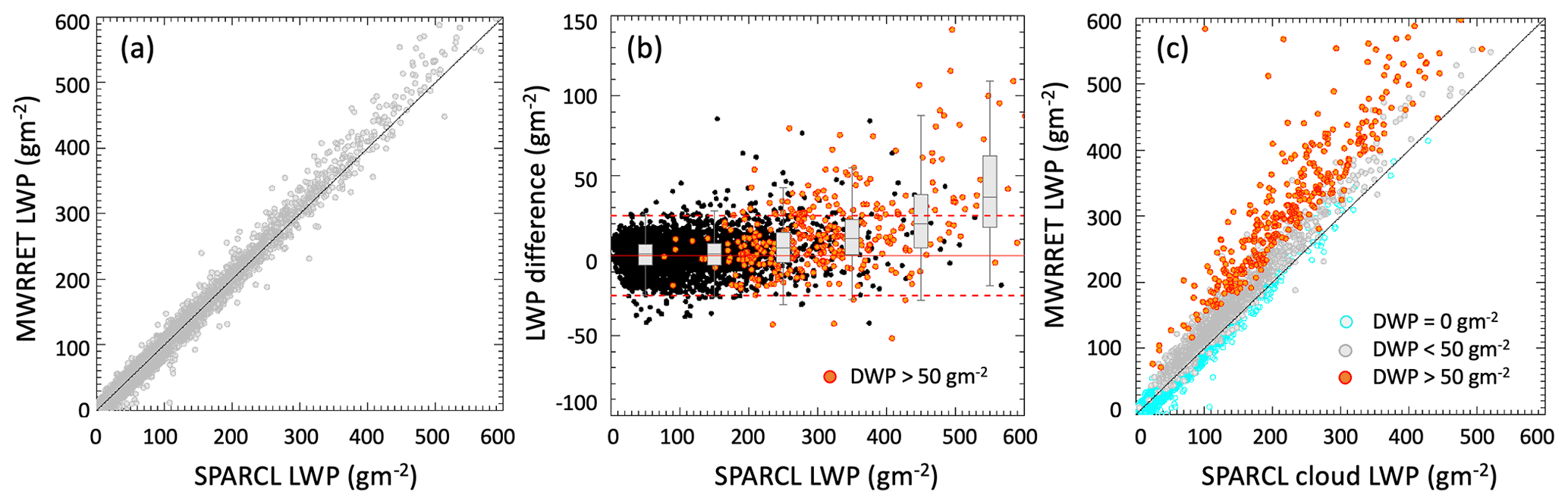
Figure A1 (a) Scatterplot between total LWP in this work (SPARCL) and physical retrieval (MWRRET) LWP. (b) Difference between the two retrievals (MWRRET minus SPARCL) for all samples (black) and samples with below-cloud drizzle water path greater than 50 g m⁻² (orange). The dashed horizontal orange lines indicate ±25 g m⁻². (c) Scatterplot between SPARCL cloud water path and MWRRET LWP. Colors represent cases with no drizzle (cyan), drizzle water path below the cloud base less than 50 g m⁻² (grey), and drizzle water path below the cloud base greater than 50 g m⁻².

Because the retrieved column integrated values of liquid water and water vapor form the basis of this work, we compare SPARCL retrievals to the traditional LWP product (MWRRET; Turner et al., 2007) available in the ARM archive. Traditionally, the total LWP retrieved by radiometers is assumed to represent the cloud water path; however, in the presence of drizzle, cloud liquid water is only a component of the total LWP, and the radiometric retrievals cannot distinguish between the cloud and the below-cloud drizzle part. In the presence of drizzle drops with a diameter larger than ∼ 100 µm, the brightness temperature at 90 GHz is affected by Mie scattering effects that, if not interpreted properly, can result in an overestimation of the LWP. A comparison between the two retrievals is shown in Fig. A1. In the following discussion only boundary layer clouds with a cloud fraction from the ceilometer greater than 0.99 were selected (total of 3580 h). As evident from Fig. A1a, the new LWP compares very well with the traditional optimal estimation retrieval (MWRRET) available in the ARM archive (Turner et al., 2007; Cadeddu et al., 2013). Looking closer, the subtle differences between the two retrievals are apparent when the LWP is higher than 300 g m⁻². This is better visualized in Fig. A1b where differences between the retrievals are displayed as a function of LWP. When the drizzle water path below cloud is higher than 50 g m⁻², MWRRET (which assumes all the hydrometeors are in the Rayleigh scattering regime) overestimates LWP because of the neglect of scattering effects from larger hydrometeors. As shown in Fig. A1c, even in the presence of light precipitation, the amount of drizzle water in clouds is non-negligible, and the total LWP coincides with the cloud water path only in non-drizzling clouds (cyan points in Fig. A1c). When drizzle is formed, however, attributing the entire column to cloud drops leads to an incorrect interpretation of the data. It should be noted that the SPARCL retrieval algorithm also derives the in-cloud drizzle water path, and hence the total drizzle water path (in cloud and below cloud) is greater than that derived from the retrievals using data from active sensors such as the radars and lidars.

The large dataset gives us an opportunity to analyze cloud adiabaticity at the site by estimating the ratio between the retrieved LWP and the LWP calculated using the adiabatic assumption for cases coincident to radiosondes (Zuidema et al., 2005; Albrecht et al., 1990). The quantities necessary for the computation of the adiabatic LWP, such as cloud-top height, temperature, pressure, and humidity profiles, are taken from radiosondes, and the cloud-base height is taken from the ceilometer. A total of 304 points satisfied all the necessary requirements for the comparison (absent or weak precipitation, marine condition, coincident radiosonde, cloud fraction >0.99) and are shown in Fig. A2 and in Table A1.

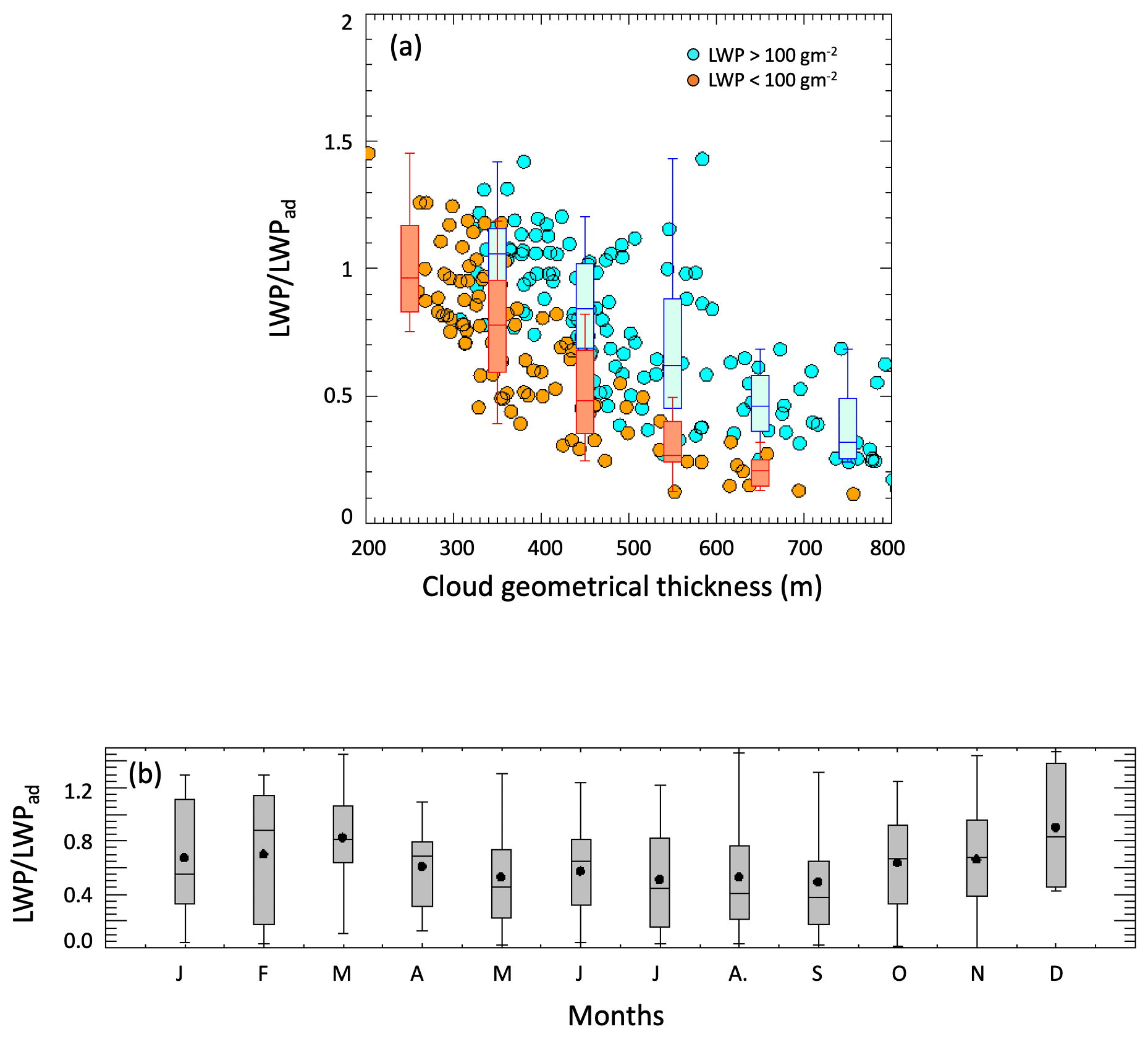
Figure A2 (a) Adiabaticity of sampled clouds against geometrical thickness for cloud with 50 < LWP < 100 g m⁻² (orange) and >100 g m⁻² (cyan). (b) Annual cycle of adiabaticity.

Table A1 Adiabaticity of sampled clouds and geometrical thickness (H). LWP_ad is the liquid water path calculated using the adiabatic assumption.

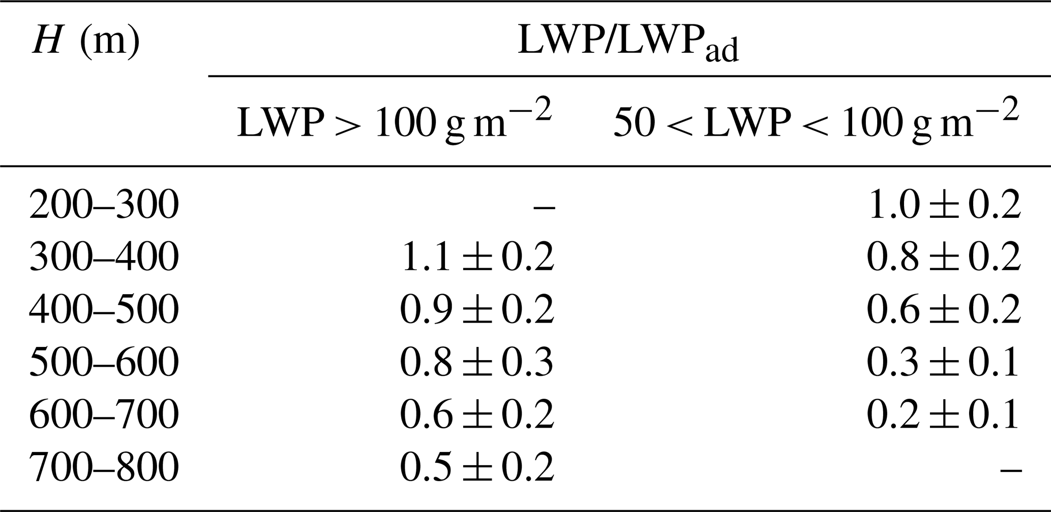
Clouds appear to be increasingly sub-adiabatic with increasing cloud geometrical thickness, are on average slightly more adiabatic, and display higher variability in winter than in summer (Fig. A2, bottom).

These results are consistent with previous observations that evidenced the mostly sub-adiabatic nature of marine clouds (e.g., Min et al., 2012, over the south pacific and Wu et al., 2020, at the ENA site). In this dataset precipitation does not seem to influence the degree of sub-adiabaticity, leading to the speculation that entrainment of dry upper-tropospheric air may be the main reason for the departure from adiabatic behavior. Uncertainties in the estimation of the cloud boundaries and LWP are likely responsible for the small percentage of clouds that become super-adiabatic. Increasing the cloud thickness of 50 m decreased the mean LWP/LWP_ad from 0.56 to 0.45 or 20 % of the calculated value. Similarly decreasing the cloud thickness of 50 m increased the mean LWP/LWP_ad from 0.56 to 0.67 or 50 %. It is therefore likely that, in addition to the uncertainty in LWP, uncertainty in cloud boundaries affects the calculations.