the Creative Commons Attribution 4.0 License.
the Creative Commons Attribution 4.0 License.
 | 10 Jan 2023
A change in the relation between the Subtropical Indian Ocean Dipole and the South Atlantic Ocean Dipole indices in the past four decades
Lejiang Yu
Shiyuan Zhong
Timo Vihma
Cuijuan Sui
Bo Sun
We utilized the global atmospheric reanalysis ERA5 and reconstructed sea surface temperature (SST) data from 1979 through 2020 to examine the stability of the relationship between the SST oscillations in the southern Indian Ocean and the Atlantic Ocean, as described by the Subtropical Indian Ocean Dipole (SIOD) and South Atlantic Ocean Dipole (SAOD) indices, respectively. We note a significant positive correlation between the two indices prior to the year 2000 but practically no correlation afterwards. We show that in the two decades prior to 2000, a positive phase of the SAOD is associated with more convective activities over the subtropical southern Atlantic Ocean and eastern Brazil, which trigger a stronger upper-atmosphere wavetrain. This produces stronger southern subtropical highs and surface anti-cyclonic circulations and therefore a stronger correlation between the two indices. The situation is reversed after 2000. Our results are potentially applicable to predictions of precipitation in southern Africa and South America.
- Article
(11043 KB) - Full-text XML
-
Supplement
(558 KB) - BibTeX
- EndNote


A southwest–northeast-oriented dipole mode characterizes the anomalous sea surface temperature (SST) patterns over the subtropical South Indian and Atlantic oceans (Wang, 2010). The former is referred to as the Subtropical Indian Ocean Dipole (SIOD) mode (Behera and Yamagata, 2001) and the latter is named the South Atlantic Ocean Dipole (SAOD) mode (Venegas et al., 1997). The two subtropical modes display similar seasonal variabilities, with their peaks occurring in austral summer (Morioka et al., 2012). Surface latent heat flux anomalies play a vital role in their variability (Sterl and Hazeleger, 2003; Suzuki et al., 2004; Hermes and Reason, 2005). Moreover, the interannual variability of the two modes has been linked to the El Niño–Southern Oscillation (ENSO) (Boschat et al., 2013). The two subtropical modes exert a great influence on precipitation in Africa and South America (Reason, 2001, 2002; Vigaud et al., 2009; Nnamchi and Li, 2011; Morioka et al., 2012; Wainer et al., 2020) and, therefore, understanding the relationship between the two modes has practical implications for precipitation forecasts in Africa and South America on a seasonal scale and beyond.
Using observational data, Fauchereau et al. (2003) noted the co-variability of the SIOD and SAOD indices in austral summer. Hermes and Reason (2005) confirmed the co-variability of the two indices and attributed it to an anomalous subtropical high. Both studies suggested a linkage between the two indices and an atmospheric zonal wavenumber-4 pattern in the Southern Hemisphere. Lin (2019) also suggested that an atmospheric zonal wavenumber-4 pattern controls the South Atlantic–South Indian Ocean SST pattern. The atmospheric wavenumber-4 pattern was also observed in other studies (Chiswell, 2021; Senapati et al., 2022a). The global wavenumber-4 SST pattern includes southern subtropical Indian Ocean and Atlantic Ocean components that resemble the two subtropical dipole modes (Senapati et al., 2021). The linkage between the SST patterns in the Southern Hemisphere ocean basins and their relation with the atmospheric wavenumber-4 pattern is a challenging and active research topic worthy of further investigation.
Although previous studies have suggested that a relationship exists between the SIOD and SAOD indices, few have focused on the stability of this relationship. In this study, we examine the SIOD–SAOD relationship over the past four decades, from 1979 through 2020. We underscore a change in the relationship that occurred around 2000 and provide a physical explanation for the change.
Monthly SST data from the United States National Oceanic and Atmospheric Administration (NOAA) Extended Reconstructed SST V5 (Huang et al., 2017) are the primary dataset utilized to calculate the SIOD and SAOD indices. A secondary SST dataset, the Kaplan Extended SST V2 dataset from the UK Met Office (Kaplan et al., 1998), is also used to confirm the results. Following previous studies, we derive the SIOD index as the difference in SST anomalies between the western (55–65∘ E, 37–27∘ S) and eastern (90–100∘ E, 28–18∘ S) subtropical Indian Ocean (Behera and Yamagata, 2001), and the SAOD index as the difference in SST anomalies between the south-western (10–30∘ W, 30–40∘ S) and north-eastern (0–20∘ W, 15–25∘ S) South Atlantic Ocean (Morioka et al., 2011). Atmospheric data from the European Centre for Medium-Range Weather Forecasts (ECMWF) fifth-generation reanalysis (ERA5, Hersbach et al., 2020) provide the upper-level (200 hPa) and surface atmospheric variables used in our analyses except for the monthly top-of-atmosphere (TOA) outgoing long-wave radiation (OLR), which is from the NOAA Interpolated OLR dataset (Liebmann and Smith, 1996). For SST or atmospheric variables, the anomalies refer to the departure from their climatology computed as the 42-year averaged value.
Correlation and regression analyses are utilized to examine the relationship between the SIOD and the SAOD indices. The confidence levels are determined by the two-tailed Student's t test. Before the correlation or regression analyses are applied to the data, the variables and indices are detrended. We also remove the influence from the ENSO signal using the method proposed by An (2003), where the ENSO signal is represented by the Niño 3.4 index. The generation and propagation of planetary waves are identified on the basis of the Rossby wave source (RWS) and the wave activity flux (WAF). The RWS is calculated following Sardeshmukh and Hoskins (1988), and the WAF is derived using the method of Takaya and Nakamura (2001). Notice that, because the peaks in the SIOD and SAOD occur in February (Morioka et al., 2012), the austral seasons in this study refer to summer (January–March), autumn (April–June), winter (July–September), and spring (October–December).
The detrended SST anomalies regressed onto the SIOD and SAOD display southwest–northeast-oriented dipoles in the subtropical southern Indian Ocean (Fig. 1a) and Atlantic Ocean (Fig. 1b). The correlation between the SIOD and SAOD indices over the 42-year period is 0.56 for austral summer (p<0.05), but it becomes insignificant in other seasons, with correlation coefficients dropping by nearly half to 0.23 for austral autumn and winter and 0.25 for austral spring. Removing the ENSO signal resulted in small changes in the correlations and their seasonal variations, with summer being the only season when the two indices are significantly correlated (0.45, p<0.01) (Fig. 1c). The Kaplan Extended SST V2 data yielded similar results, with slightly lower summertime correlation coefficients of 0.49 (with the ENSO signal) and 0.38 (without the ENSO signal, p<0.05). Henceforth, we focus on the summer time series without the ENSO signal.
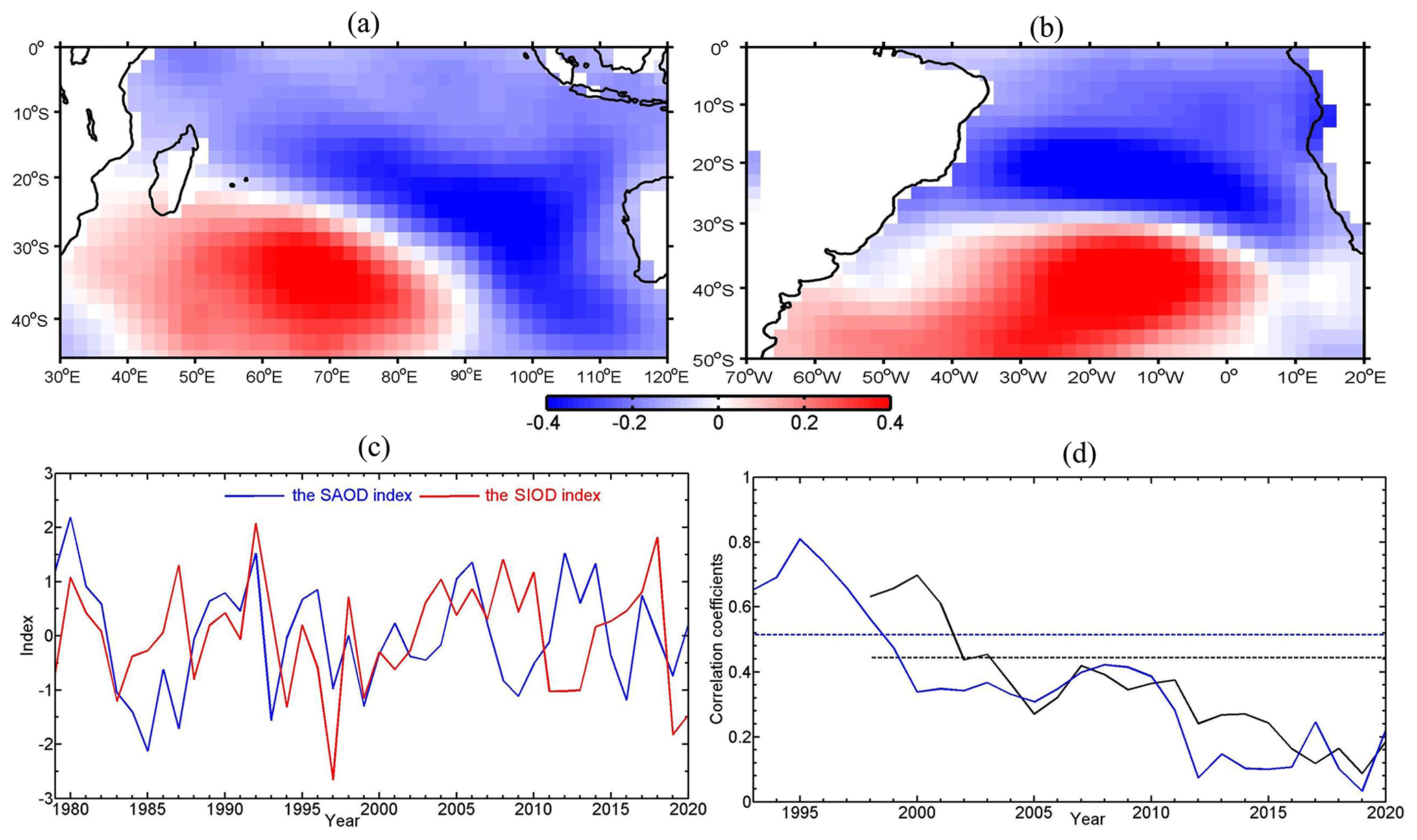
Figure 1Regression patterns of austral summer (JFM) SST anomalies (∘C) on the positive phases of the summertime indices of (a) the Subtropical Indian Ocean Dipole (SIOD) and (b) the South Atlantic Ocean Dipole (SAOD), (c) their time coefficients, and (d) the moving correlations between the detrended and ENSO-signal-removed SIOD and SAOD indices (time coefficients) using a 20-year (solid black line) and a 15-year (solid blue line) sliding window. In (d), the dashed lines denote the correlation coefficients with the 95 % confidence level for 20 (black) and 15 (blue) samples, and the abscissa indicates the end year of the moving correlations. The above results were derived using the NOAA Extended Reconstructed SST V5 data.
To assess the stability of the SIOD–SAOD correlation over the past four decades, we calculate the moving correlation of the two indices using 15-year and 20-year sliding windows (Fig. 1d). For the 15-year window, the correlation is above (below) the 95 % confidence level before (after) 1998, and for the 20-year sliding window, the shifting occurs in 2003. Similar results are obtained using the Kaplan Extended SST V2 data (Fig. 2). There is a remarkable difference in the correlation between the two indices prior to and after 1999 (Fig. 1d). For the 1979–1999 period, the correlation coefficient is 0.64 (p<0.01), but it drops sharply to only 0.19 (p>0.05) for the 2000–2020 period. Results derived using the Kaplan Extended SST V2 data are very similar, with correlation coefficients of 0.60 (p<0.01) for the 1979–1999 period and 0.20 (p>0.05) for the 2000–2020 period. This notable drop in the correlation between the SIOD and SAOD indices from the first two decades to the next two warrants further investigation. Below we explore the reasons behind the change.
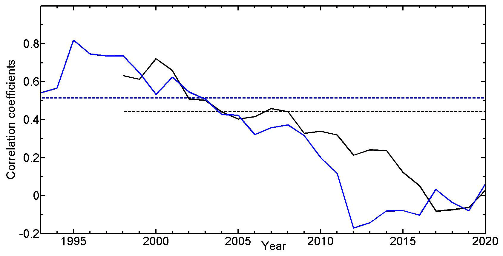
Figure 2Moving correlations of the detrended and ENSO-signal-removed SIOD and SAOD indices using a 20-year (solid black line) and a 15-year (solid blue line) sliding window. Dashed lines denote the correlation coefficients with the 95 % confidence level for 20 (black) and 15 (blue) samples. The abscissa indicates the end year of the moving correlations. The above results were obtained using the Kaplan Extended SST V2 data.
We compare the regression maps of the Southern Hemisphere SST anomalies on the summertime SAOD and SIOD indices for the 1979–1999 period with those for the 2000–2020 period (Fig. 3). There are clear differences in the anomalous SST patterns between the two periods. As a response to the positive phase of the SAOD index, significant SST anomalies occur in the southern subtropical Indian Ocean during the 1979–1999 period, with the spatial pattern (Fig. 3a) closely resembling the positive-phase SIOD index (Fig. 1a); however, the SST anomalies for the 2000–2020 period are not significant in the southern subtropical Indian Ocean (Fig. 3b). Similarly, corresponding to the SIOD index, a dipole of significant SST anomalies that appears in the South Atlantic Ocean (Fig. 3c) for the 1979–1999 period bears a strong resemblance to the positive-phase SAOD pattern (Fig. 1b), whereas for the 2000–2020 period, the SST anomalies are insignificant (Fig. 3d). These results confirm the strong correlation between the SAOD and SIOD indices during the first two decades and the lack of correlation in the last two decades (i.e. since the turn of the century). The SST anomalies in Fig. 3 display the appearance of the SST wavenumber-4 mode (Senapati et al., 2021), including the SIOD and SAOD patterns. Senapati et al. (2022b) suggested that the weakening of the SST wavenumber-4 pattern after 2000 is related to the South Pacific Meridional Mode. In addition, the weaker SIOD–SAOD relationship after 2000 may be related to the decadal variability of a warm pool dipole, with opposite SST anomalies in the southeastern Indian Ocean and the western-central tropical Pacific Ocean (Zhang et al., 2021).
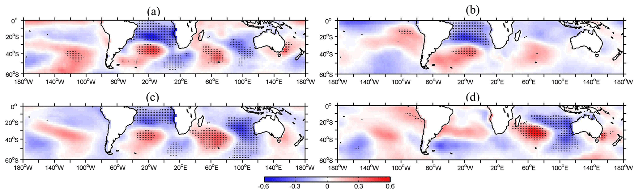
Figure 3Regression maps of the SST anomalies (∘C) on the summertime indices of (a, b) SAOD and (c, d) SIOD over the periods of (a, c) 1979–1999 and (b, d) 2000–2020. Dots denote the regions where the confidence level is above 95 %.
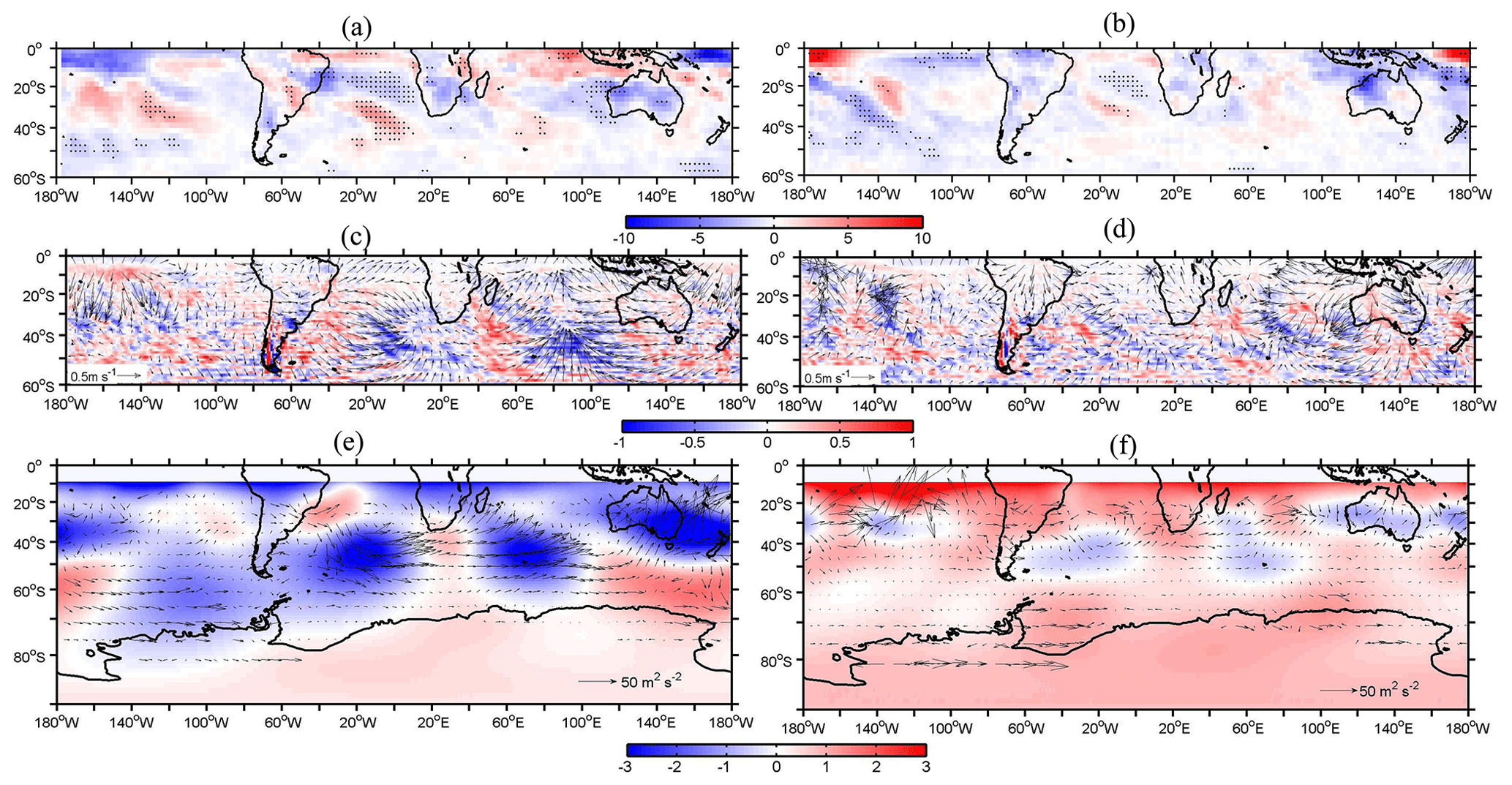
Figure 4Regression maps of (a, b) the anomalous outgoing long-wave radiation (OLR) (W m−2) at the top of the atmosphere, (c, d) the Rossby wave sources (RWSs) (10−10 s−2) and 200 hPa divergent wind (vectors), and (e, f) the wave activity flux (WAF) (vector) and streamfunction (m2 s−1) on the summertime SAOD index over the periods of (a, c, e) 1979–1999 and (b, d, f) 2000–2020.
Lin (2019) related a South Atlantic–South Indian Ocean pattern to a wavetrain induced by the South Atlantic Convergence Zone anomaly. We hypothesize that the stability of the SAOD–SIOD relation may also be related to the strength of the wavetrain. To test this hypothesis, we examine the regression patterns of several atmospheric variables related to convective and wave activities (OLR, RWS, WAF, 200 hPa divergent wind, and streamfunction) to the SAOD index in austral summer separately for the 1979–1999 period and the 2000–2020 period (Fig. 4). Over the 1979–1999 period, corresponding to the positive phase of the SAOD index, convective activities are enhanced over the southern subtropical Atlantic Ocean and eastern Brazil, which are flanked by suppressed convective activities over the tropical and mid-latitude South Atlantic Ocean (Fig. 4a). The convective activities over the western subtropical southern Atlantic Ocean and eastern Brazil produce a positive RWS and 200 hPa divergent wind (Fig. 4c), which trigger a wavetrain propagating south-eastwards into the South Atlantic Ocean and then eastwards into the South Indian Ocean, Australia and the South Pacific Ocean (Fig. 4e). The wavetrain generates negative streamfunction anomalies over the South Indian and Atlantic oceans (Fig. 4e). In contrast, over the 2000–2020 period, the magnitude of the anomalous OLR is less significant than that over the 1979–1999 period (Fig. 4b). A weaker RWS and upper-level divergent wind (Fig. 4d) indicate a weaker wavetrain, which results in weaker streamfunction anomalies over the South Atlantic and Indian oceans (Fig. 4f). To clearly show the RWS, upper-level divergent wind and Rossby wavetrain, we show the significant areas in Fig. 4c–f in a supplementary file (Fig. S1 in the Supplement).

Figure 5Climatological OLR anomalies (W m−2) during (a) 1979–1999 and (b) 2000–2020 with respect to the 42-year climatology over the 1979–2020 period.
Although the magnitudes of the OLR anomalies related to the SAOD index are comparable over the two periods (Fig. 4a and b), the anomalous OLR and RWS and the related wavetrain associated with the SAOD index are substantially different between the two periods. The differences in the climatological conditions over the two periods may provide a plausible explanation. For example, over the subtropical southern Atlantic Ocean and most of Brazil, the climatological OLR anomalies are generally negative during the 1979–1999 period, suggesting stronger convective activity, which is favourable for the generation of the wavetrain (Fig. 5a); in contrast, OLR anomalies are mostly positive during 2000–2020, indicating suppressed convective activities, which is unfavourable for the formation of the wavetrain (Fig. 5b). Thus, the interdecadal variability of the OLR activities can modulate the effect of the SAOD mode on atmospheric circulation patterns over other ocean basins.
The SAOD and SIOD modes are related to the subtropical highs in the South Atlantic and Indian Oceans, with stronger highs corresponding to the positive phases of the two indices due to wind-induced evaporation (Wang, 2010; Behera and Yamagata, 2001; Venegas et al., 1997). We now proceed to examine the climatological mean sea level pressure and surface wind field related to the aforementioned wavetrain over the two periods (Fig. 6). The positions and strengths of the climatological subtropical highs and the associated surface winds in the southern Indian Ocean and the Atlantic Ocean show little difference when the two periods are compared (Fig. 6a and b). However, the regression of the mean sea level pressure on the SAOD index for the two periods shows considerably stronger subtropical highs and anti-cyclonic circulations in the South Atlantic and the Indian Ocean over the 1979–1999 period than the 2000–2020 period (Fig. 6c and d). According to the study of Hermes and Reason (2005), a stronger subtropical high favours larger magnitudes of the SST anomalies represented by the SAOD and SIOD indices. The large decrease in the strength of the summertime subtropical high associated with SAOD from the first two decades to the next two (Fig. 6c and d) corroborates the sharp drop in the SAOD–SIOD correlation (Fig. 1d). Prior to 2000, the stronger wavetrain associated with SAOD induced stronger summertime subtropical highs, which produced larger subtropical SST anomalies in both basins, strengthening the SASD–SIOD relationship. After 2000, the weaker wavetrain induced weaker subtropical highs. The SST anomalies in each basin are largely determined by the physical processes in each basin, which are not directly related to the wavetrain. Thus, the SAOD–SIOD relationship is weaker after 2000.
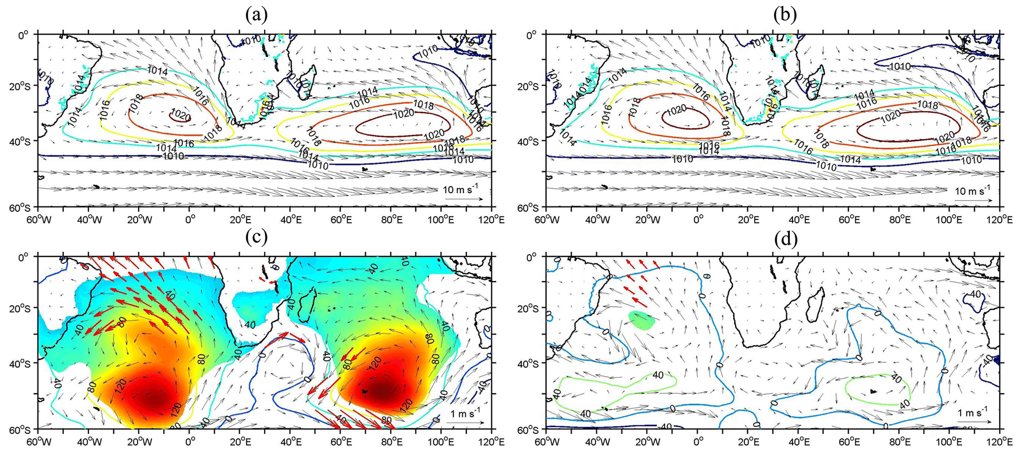
Figure 6Climatological mean sea level pressure (MSLP, in hPa) and the 10 m wind field (vector) over the periods of (a) 1979–1999 and (b) 2000–2020, and regression maps of MSLP (in Pa) and the 10 m wind field (vector) on the summertime SAOD index over the periods of (c) 1979–1999 and (d) 2000–2020. Shaded regions and red vectors indicate that the confidence level is above 95 %.
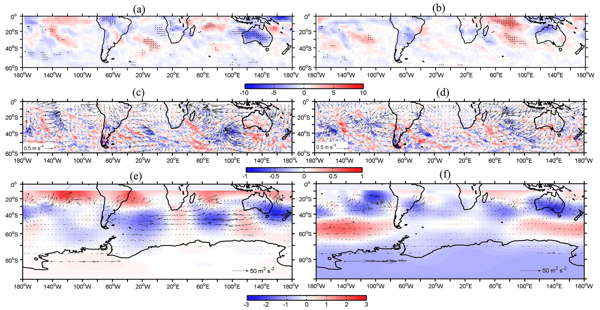
Figure 7Regression maps of (a, b) the OLR (W m−2), (c, d) the RWS (10−10 s−2) and the 200 hPa divergent wind (vector), and (e, f) the WAF (vector) and streamfunction (m2 s−1) on the summertime SIOD index over the 1979–1999 period (a, c, e) and the 2000–2020 period (b, d, f).
Similarly, we have also obtained the patterns of the aforementioned atmospheric circulation variables associated with the SIOD index separately for the two periods (Fig. 7). During 1979–1999, negative OLR anomalies occur over northern South America, corresponding to upper-level divergent wind and positive RWS anomalies, while positive OLR anomalies exist over the southern Atlantic Ocean, leading to upper-level convergent wind and negative RWS anomalies (Fig. 7a and c). Those anomalous RWSs produce an anomalous Rossby wavetrain propagating from the southern Atlantic Ocean to the southern Indian Ocean (Fig. 7e). During 2000–2020, negative (positive) OLR anomalies over the tropical (subtropical) central Pacific Ocean generate anomalous upper-level winds and RWSs, which excite a wavetrain propagating from the Pacific to South America and the southwestern South Atlantic Ocean (Fig. 7b, d, and f). Meanwhile, stronger convective activities over the southwestern Indian Ocean and weaker convective activities over the central Indian Ocean also produce anomalous RWSs, which trigger a local wavetrain propagating eastwards into Australia. However, the two wavetrains are controlled by different factors and are not connected to each other over the South Atlantic Ocean. We also examine the MSLP and surface wind field related to the SIOD index in austral summer for the 1979–1999 and 2000–2020 periods (Fig. 8). Over the 1979–1999 period, stronger subtropical highs develop over the South Indian and Atlantic oceans, which induce the positive phases of the SIOD and SAOD modes, respectively (Fig. 8a), suggesting that the SIOD and SAOD indices are connected to each other through the aforementioned wavetrain (Fig. 7e). Over the 2000–2020 period, positive MSLP anomalies and anomalous anti-cyclonic circulation dominate over the South Indian Ocean, though negative MSLP anomalies and anomalous cyclonic circulation occur over the southwestern South Indian Ocean (Fig. 8b). The atmospheric circulation anomalies over the South Indian Ocean are related to the OLR anomalies and induce a local wavetrain (Fig. 7b, d and f). Similarly, the significant areas in Fig. 7c–f are shown in a supplementary file (Fig. S1). The positive MSLP anomalies and anti-cyclonic circulation anomalies are absent over the South Atlantic Ocean (Fig. 8b). These results indicate that the SIOD mode over the 2000–2020 period is related to local convective activities, not to those over the South Atlantic Ocean.
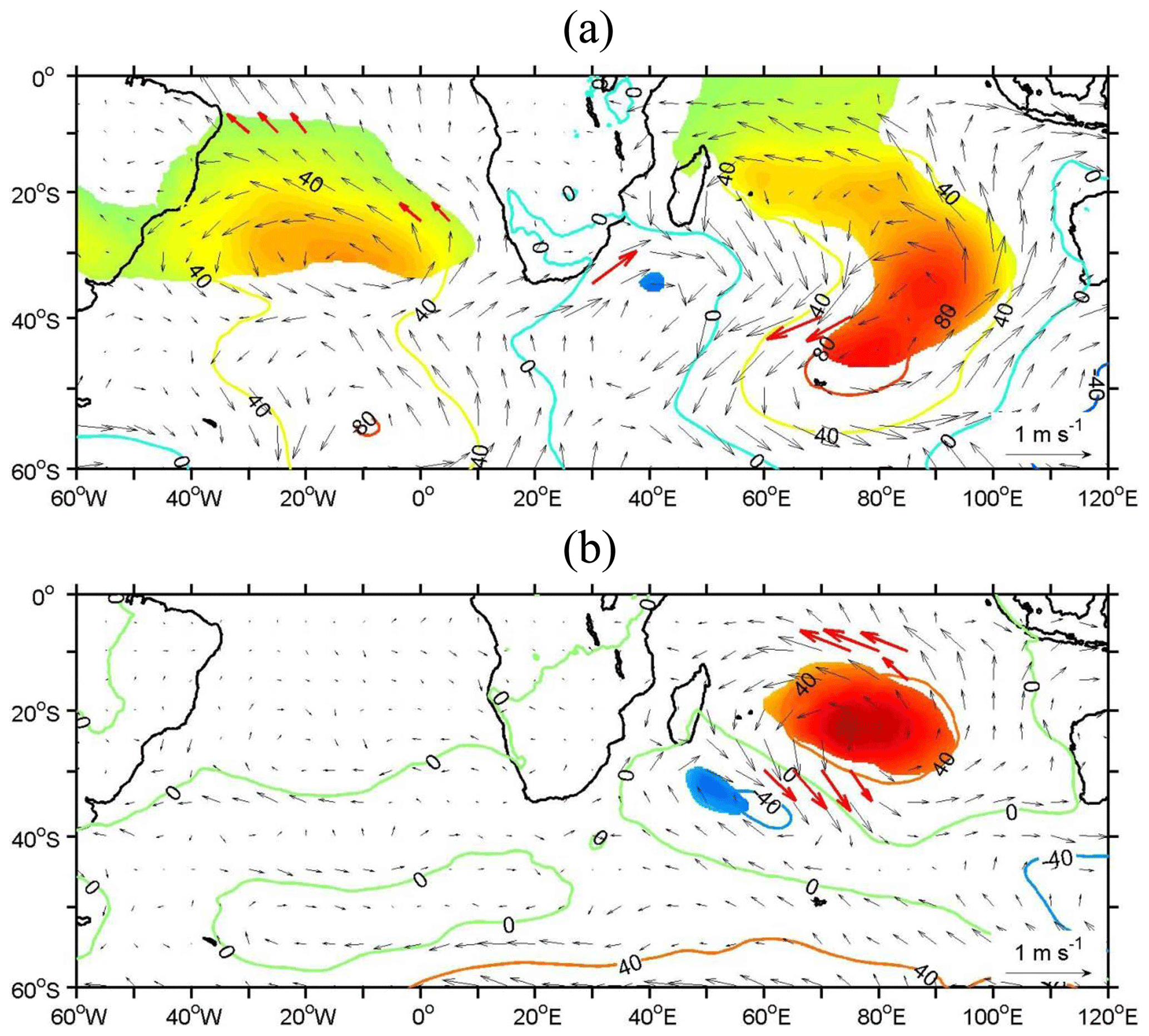
Figure 8Regression maps of MSLP (in Pa) and the 10 m wind field (vector) onto the summertime SIOD index over the periods of (a) 1979–1999 and (b) 2000–2020. Shaded regions and red vectors indicate that the confidence level is above 95 %.
In this study, we examined the relation between the oscillations of the SST in the subtropical South Indian and Atlantic oceans – described by the SIOD and SAOD indices, respectively – and the stability of this relation using the ERA5 global atmospheric reanalysis and reconstructed SST data from 1979 through 2020. We found a significant relation between the two indices in austral summer. Through moving correlation analyses, we discovered that the relation in austral summer was not stable for the past four decades. Specifically, the correlation between the two indices was significant prior to 2000 but insignificant afterwards. The change in the relation between the two indices is attributed to a change in the strength of the atmospheric wavetrain induced by anomalous convective activity over the subtropical southern Atlantic Ocean and eastern Brazil. More frequent and stronger convective activities prior to 2000 excited a stronger wavetrain, which produced stronger subtropical highs during the positive phase of the SAOD, resulting in a stronger relation between the two indices. The opposite occurred after 2000.
The interdecadal variability of the OLR over the subtropical South America and Atlantic Ocean is the key to the relation between the SAOD and SIOD indices. What determined the OLR anomalies in the region prior to and after 2000 needs to be further investigated. Hermes and Reason (2005) suggested that the southern subtropical high is related to the Antarctic Oscillation (AAO), and the linkage strengthened after the mid-1970s. The influence of the change in the AAO index on the relation between the SAOD and the SIOD indices needs to be assessed. Yu et al. (2017) noted a phase change of the Atlantic Multidecadal Oscillation (AMO) and the Pacific Decadal Oscillation (PDO) indices in the late 1990s, with the PDO shifting from positive to negative and the AMO switching from negative to positive around 1999. Dong and Dai (2015) noted the influence of the IPO (interdecadal pacific oscillation) on precipitation in Brazil. However, the influence from the same phase of the IPO has great uncertainty and depends on the period and dataset (Dong and Dai, 2015). Jones and Carvalho (2018) suggested that there was more precipitation in Brazil during the negative phase of the AMO than during its positive phase. Longer datasets are utilized to examine the effects of the IPO and AMO on convective activity over the subtropical South America and Atlantic Ocean at the interdecadal timescale. Although our results are only based on statistical analyses, they have the potential to improve the prediction of precipitation in southern Africa and South America.
The monthly SST data from the US NOAA Extended Reconstructed Sea Surface Temperature (ERSST) version 5 (ERSST v5) are available online (https://www1.ncdc.noaa.gov/pub/data/cmb/ersst/v5/netcdf/; NOAA, 2021). Kaplan Extended SST V2 data are derived from the website https://psl.noaa.gov/cgi-bin/db_search/DBSearch.pl?Dataset=Kaplan+Extended+SST+V2&Variable=Sea+Surface+Temperature (NOAA, 2022). The monthly ERA5 reanalysis data are available from the Copernicus Climate Data Store (https://www.ecmwf.int/en/forecasts/datasets/reanalysis-datasets/era5; ECMWF, 2022). The monthly OLR data are derived from the NOAA Interpolated OLR (https://psl.noaa.gov/cgi-bin/db_search/DBSearch.pl?Dataset=NOAA+Interpolated+OLR&Variable=Outgoing+Longwave+Radiation; NOAA, 2020).
Codes are available from the corresponding author on reasonable request.
The supplement related to this article is available online at: https://doi.org/10.5194/acp-23-345-2023-supplement.
LY designed the research, analysed the data, and wrote the first draft of the paper. SZ and TV revised the first draft and provided useful insights during various stages of the work. CS and BS provided some comments and helped with editing the paper.
The contact author has declared that none of the authors has any competing interests.
Publisher's note: Copernicus Publications remains neutral with regard to jurisdictional claims in published maps and institutional affiliations.
We thank the European Centre for Medium-Range Weather Forecasts (ECMWF) for the ERA-5 data.
This study is financially supported by the National Key R & D Program of China (2022YFE0106300), the National Science Foundation of China (41941009), and the European Commission H2020 project Polar Regions in the Earth System (PolarRES; Grant 101003590).
This paper was edited by Peter Haynes and reviewed by two anonymous referees.
An, S. I.: Conditional maximum covariance analysis and its application to the tropical Indian Ocean SST and surface wind stress anomalies, J. Climate, 16, 2932–2938, 2003.
Behera, S. K. and Yamagata, T.: Subtropical SST dipole events in the southern Indian Ocean, Geophys. Res. Lett., 28, 327–331, 2001.
Boschat, G, Terray, P., and Masson, S.: Extratropical forcing of ENSO, Geophys. Res. Lett., 40, 1605–1611, 2013.
Chiswell, S. M.: Atmospheric wavenumber-4 driven South Pacific marine heat waves and marine cool spells, Nat. Commun., 12, 4779, https://doi.org/10.1038/s41467-021-25160-y, 2021.
Dong, B. and Dai, A.: The influence of the Interdecadal Pacific Oscillation on temperature and precipitation over the global, Clim. Dynam., 45, 2667–2681, 2015.
ECMWF: ERA5, https://www.ecmwf.int/en/forecasts/datasets/reanalysis-datasets/era5, last access: 10 August 2022.
Fauchereau, N., Trzaska, S., Richard, Y., Roucou, P., and Camberlin, P.: Sea Surface temperature co-variability in the Southern Atlantic and Indian Oceans And its connections with the atmospheric circulation in the Southern Hemisphere, Int. J. Climatol., 23, 663–677, 2003.
Hermes, J. C. and Reason, C. J. C.: Ocean model diagnosis of interannual coevoling SST variability in the South Indian and South Atlantic Oceans, J. Climate, 18, 2864–2882, 2005.
Hersbach, H., Bell, B., Berrisford, P., Hirahara, S., Horányi, A., Muñoz-Sabater, J., Nicolas, J., Peubey, C., Radu, R., Schepers, D., Simmons, A., Soci, C., Abdalla, S., Abellan, X., Balsamo, G., Bechtold, P., Biavati, G., Bidlot, J., Bonavita, M., De Chiara, G., Dahlgren, P., Dee, D., Diamantakis, M., Dragani, R., Flemming, J., Forbes, R., Fuentes, M., Geer, A., Haimberger, L., Healy, S., Hogan, J. R., Hólm, E., Janisková, M., Keeley, S., Laloyaux, P., Lopez, P., Lupu, C., Radnoti, G., de Rosnay, P. Rozum, I., Vamborg, F., Villaume, S., and Thépaut J.-N.: The ERA5 global reanalysis, Q. J. Roy. Meteorol. Soc., 146, 1999–2049, 2020.
Huang, B., Thorne, P. W., Banzon,V. F., and Zhang, H. M.: Extended Reconstructed SeaSurface Temperature version 5 (ERSSTv5), Upgrades, validations, and Intercomparisons, J. Climate, 30, 8179–8205, 2017.
Jones, C. and Carvalho, L. M. V.: The influence of the Atlantic multidecadal oscillation on the eastern Andes low-level jet and precipitation in South America, npj Clim. Atmos. Sci., 1, 40, https://doi.org/10.1038/s41612-018-0050-8, 2018.
Kaplan, A., Cane, M., Kushnir, Y., Clement, A., Blumenthal, M., and Rajagopalan, B.: Analyses of global sea surface temperature 1856–1991, J. Geophys. Res., 103, 18567–18589, 1998.
Liebmann, B. and Simth, C. A.: Description of a complete (interpolated) outgoinglongwave radiation dataset, B. Am. Meteorol. Soc., 77, 1275–1277, 1996.
Lin, Z.: The South Atlantic-South Indian Ocean: a zonally oriented teleconnection along the Southern Hemisphere westerly jet in austral summer, Atmosphere, 10, 259, https://doi.org/10.3390/atmos10050259, 2019.
Morioka, Y., Tozuka, T., and Yamagata, T.: On the growth and decay of the subtropical dipole mode in the south Atlantic, J. Climate, 24, 5538–5554, 2011.
Morioka, Y., Tozuka, T., Masson, S., Terray, P., Luo, J.-J., and Yamagata, T.: Subtropical dipole modes simulated in a coupled general circulation mode, J. Climate, 25, 4029–4047, 2012.
Nnamchi, H. C. and Li, J. P.: Influence of the South Atlantic Ocean Dipole on West African summer precipitation, J. Climate, 24, 1184–1197, 2011.
NOAA: Gridded Climate Data, https://psl.noaa.gov/cgi-bin/db_search/DBSearch.pl?Dataset=NOAA+Interpolated+OLR&Variable=Outgoing+Longwave+Radiation, last access: 6 July 2020.
NOAA: Index of /pub/data/cmb/ersst/v5/netcdf, NOAA [data set] https://www1.ncdc.noaa.gov/pub/data/cmb/ersst/v5/netcdf/, last access: 20 December 2021.
NOAA: Gridded Climate Data, https://psl.noaa.gov/cgi-bin/db_search/DBSearch.pl?Dataset=Kaplan+Extended+SST+V2&Variable=Sea+Surface+Temperature, last access: 29 June 2022.
Reason, C. J. C.: Subtropical Indian Ocean SST dipole events and southern African rainfall, Geophys. Res. Lett., 28, 2225–2227, 2001.
Reason, C. J. C.: Sensitivity of the southern African circulation to dipole sea-surface temperature patterns in the South Indian Ocean, Int. J. Climatol., 22, 377–393, 2002.
Sardeshmukh, P. D. and Hoskins, B. J.: The generation of global rotational flow by steady idealized tropical divergence, J. Atmos. Sci., 45, 1228–1251, 1988.
Senapati, B., Dash, M. K., and Behera, S. K.: Global wave number-4 pattern in the southern subtropical sea surface temperature, Scient. Rep., 11, 142, https://doi.org/10.1038/s41598-020-80492-x, 2021.
Senapati, B., Deb, P., Dash, M. K., and Behera, S. K.: Origin and dynamics of global atmospheric wavenumber-4 in the Southern mid-latitude during austral summer, Clim. Dynam., 59, 1309–1322, 2022https://doi.org/10.1007/s00382-021-06040-z, 2022a.
Senapati, B., Dash, M. K., and Behera, S. K.: Decadal variability of southern subtropical SST wavenumber-4 pattern and its impact, Geophys. Res. Lett., 49, e2022GL099046, https://doi.org/10.1029/2022GL099046, 2022b.
Sterl, A. and Hazeleger, W.: Coupled variability and air-sea interaction in the South Atlantic Ocean, Clim. Dynam., 21, 559–571, 2003.
Suzuki, R.,Behera, S. K., Iizuka, S., and Yamagata, T.: IndianOcean Subtropical dipoles simulated using a coupled general circulation model, J. Geophys. Res., 109, C09001, https://doi.org/10.1029/2003JC001974, 2004.
Takaya, K. and Nakamura, H.: A formulation of a phase in dependent wave-activity flux for stationary and migratory quasi geostrophic eddies on a zonally varying basic flow, J. Atmos. Sci., 58, 608–627, 2001.
Venegas, S. A., Mysak, L. A., and Straub, D. N.: Atmosphere–ocean coupled variability in the South Atlantic, J. Climate, 10, 2904–2920, 1997.
Vigaud, N., Richard, Y., Rouault, M., and Fauchereau, N.: Moisture transport between The South Atlantic Ocean and southern Africa: Relationships with summer rainfall and associated dynamics, Clim. Dynam., 32, 113–123, 2009.
Wainer, I., Prado, L. F., Khodri, M., and Otto-Bliesner, B.: The South Atlantic subtropical dipole mode since the last deglaciation and changes in rainfall, Clim. Dynam., 56, 109–122, https://doi.org/10.1007/s00382-020-05468-z, 2020.
Wang, F.: Subtropical dipole mode in the Southern Hemisphere: A global view, Geophys. Res. Lett., 37, L10702, https://doi.org/10.1029/2010GL042750, 2010.
Yu, L., Zhong, S., Winkler, J. A., Zhou, M., Lenschow, D. H., Li, B., Wang, X., and Yang, Q.: Possible connection of the opposite trends in Arctic and Antarctic sea ice cover, Scient. Rep., 7, 45804, https://doi.org/10.1038/srep45804, 2017.
Zhang, L., Han, W., Karnauskas, K. B., Li, Y., and Tozuka, T.: Eastward shift of Interannual climate variability in the South Indian Ocean since 1950, J. Climate, 35, 561–575, 2021.