the Creative Commons Attribution 4.0 License.
the Creative Commons Attribution 4.0 License.
 | 20 Mar 2023
Vehicle-based in situ observations of the water vapor isotopic composition across China: spatial and seasonal distributions and controls
Di Wang
Camille Risi
Xuejie Wang
Jiangpeng Cui
Gabriel J. Bowen
Kei Yoshimura
Zhongwang Wei
Laurent Z. X. Li
Stable water isotopes are natural tracers in the hydrological cycle and have been applied in hydrology, atmospheric science, ecology, and paleoclimatology. However, the factors controlling the isotopic distribution, both at spatial and temporal scales, are debated in low and middle latitude regions, due to the significant influence of large-scale atmospheric circulation and complex sources of water vapor. For the first time, we made in situ observations of near-surface vapor isotopes over a large region (over 10 000 km) across China in both pre-monsoon and monsoon seasons, using a newly designed vehicle-based vapor isotope monitoring system. Combined with daily and multiyear monthly mean outputs from the isotope-incorporated global spectral model (Iso-GSM) and infrared atmospheric sounding interferometer (IASI) satellite to calculate the relative contribution, we found that the observed spatial variations in both periods represent mainly seasonal mean spatial variations, but are influenced by more significant synoptic-scale variations during the monsoon period. The spatial variations of vapor δ18O are mainly controlled by Rayleigh distillation along air mass trajectories during the pre-monsoon period, but are significantly influenced by different moisture sources, continental recycling processes, and convection during moisture transport in the monsoon period. Thus, the North–South gradient observed during the pre-monsoon period is counteracted during the monsoon period. The seasonal variation of vapor δ18O reflects the influence of the summer monsoon convective precipitation in southern China and a dependence on temperature in the North. The spatial and seasonal variations in d-excess reflect the different moisture sources and the influence of continental recycling. Iso-GSM successfully captures the spatial distribution of vapor δ18O during the pre-monsoon period, but the performance is weaker during the monsoon period, maybe due to the underestimation of local or short-term high-frequency synoptic variations. These results provide an overview of the spatial distribution and seasonal variability of water isotopic composition in East Asia and their controlling factors, and they emphasize the need to interpret proxy records in the context of the regional system.
- Article
(12082 KB) - Full-text XML
-
Supplement
(2108 KB) - BibTeX
- EndNote


Stable water isotopes have been applied to study a wide range of hydrological and climatic processes (Gat, 1996; Bowen et al., 2019; West et al., 2009). This is because water isotopes vary with the water phases (e.g., evaporation, condensation), and therefore produce a natural labeling effect within the global water cycle. Stable isotopic signals recorded in natural precipitation archives are used in the reconstructions of ancient continental climate and hydrological cycles due to their strong relationship with local meteorological conditions. Examples include ice cores (Thompson, 2000; Yao et al., 1991; Tian et al., 2006), tree-ring cellulose (Liu et al., 2017), stalagmites (Van Breukelen et al., 2008), and lake deposits (Hou et al., 2007). However, unlike in polar ice cores, isotopic records in ice cores from low and middle latitude regions have encountered challenges as temperature proxies (Brown et al., 2006; Thompson et al., 1997).
The East Asian country of China is the main distribution area of ice cores in the low and middle latitudes (Schneider and Noone, 2007), where the interpretation of isotopic variations in natural precipitation archives are debated, because they can be interpreted as recording temperature (Thompson et al., 1993, 1997, 2000; Thompson, 2000), regional-scale rainfall or strength of the Indian monsoon (Pausata et al., 2011), or the origin of air masses (Aggarwal et al., 2004; Risi et al., 2010). This is because China has a typical monsoon climate, and moisture from several sources mix in this region (Wang, 2002; Domrös and Peng, 2012). In general, large parts of the country are affected by the Indian monsoon and the East Asian monsoon in summer, which bring humid marine moisture from the Indian Ocean, South China Sea, and northwestern Pacific Ocean (Fig. 1). During the non-monsoon seasons, the westerlies influence most of northern China (Fig. 1). Westerlies brings extremely cold and dry air masses. Occasional moisture flow from the Indian Ocean and/or Pacific Ocean brings moisture to southern China. Continental recycling, i.e., the moistening of the near-surface air by the evapotranspiration from the land surface (transpiration by plants, evaporation of bare soil or standing water bodies; Brubaker et al., 1993), is also an important source of water vapor in both seasons. Some of the spatial and seasonal patterns of water vapor transport are imprinted in the observed station-based precipitation isotopes (Araguás-Araguás et al., 1998; Tian et al., 2007; Gray and Wright, 1993; Mei'e et al., 1985; Tan, 2014). However, precipitation isotopes can only be obtained at a limited number of stations and only on rainy days. The lack of continuous information makes it limited to analyze the effects of water vapor propagation and alternating monsoon and westerlies. In addition, the seasonal pattern and the spatial variation of water isotopes can strongly influenced by synoptic-scale processes, through their influence on moisture source, transport, convection, and mixing processes (Klein et al., 2015; Sánchez-Murillo et al., 2019; Wang et al., 2021), which requires higher frequency observations. For example, some studies found the impact of tropical cyclones (Gedzelman, 2003; Bhattacharya et al., 2022), the boreal summer intraseasonal oscillation (BSISO) (Kikuchi, 2021), local or large-scale convections (Shi et al., 2020), cold front passages (Aemisegger et al., 2015), depressions (Saranya et al., 2018), and anticyclones (Khaykin et al., 2022) on water isotopes in the Asian region. Additional data and analysis refining our understanding of controls on the spatial and temporal variation of water isotopes in low-latitude regions therefore are needed.
Unlike precipitation, water vapor enters all stages of the hydrological cycle, experiencing frequent and intensive exchange with other water phases; in particular, it is directly linked with water isotope fractionation. Furthermore, vapor isotopes can be measured in regions and periods without precipitation, and therefore have significant potential to trace how water is transported, mixed, and exchanged (Galewsky et al., 2016; Noone, 2008), as well as to diagnose large-scale water cycle dynamics. Water vapor isotope data have been applied to various applications ranging from the marine boundary layer to continental recycling and to various geographical regions from tropical convection to polar climate reconstructions (Galewsky et al., 2016). The development of laser-based spectroscopic isotope analysis made the precise, high-resolution, and real-time measurements of both vapor δ18O and δ2H available in recent decades. However, most of the in situ observations of water vapor isotopes are also station based (e.g., Li et al., 2020; Tian et al., 2020; Steen-Larsen et al., 2017; Aemisegger et al., 2014) or performed during ocean cruises (Thurnherr et al., 2020; Bonne et al., 2019; Liu et al., 2014; Kurita, 2011; Benetti et al., 2017). One study made vehicle-based in situ observations to document spatial variations, but this was restricted to the Hawai'i island (Bailey et al., 2013). These observations provided new insight on moisture sources, synoptic influences, and sea surface evaporation fractionation processes. However, in situ observations documenting continuous spatial variations at the large continental scale do not exist. This paper presents the first isotope dataset documenting the spatial variations of vapor isotopes over a large continental region (over 10 000 km), both during the pre-monsoon and monsoon periods, based on vehicle-based in situ observations.
After describing our observed time series along the route (Sect. 3.1 and 3.2), we quantify the relative contributions of seasonal mean spatial variations and synoptic-scale variations that locally disturb the seasonal mean to our observed time series (Sect. 3.3). We show that our observed variations in both seasons are dominated by spatial variations but are influenced by significant synoptic-scale variations during the monsoon period. On the basis of this we then focus on analyzing the main mechanisms underlying these distributions (Sect. 4). Collectively, these data and analyses provide a refined understanding of how the interaction of the summer monsoon and westerly circulation controls water isotope ratios in East Asia.
2.1 Geophysical description
We conducted two campaigns to monitor vapor isotopes across a large part of China during the pre-monsoon (3 to 26 March 2019) and the monsoon (28 July to 18 August 2018) periods, using a newly designed vehicle-based vapor isotope monitoring system (Fig. S1). The two campaigns run along almost the same route, with slight deviation in the far northeast of China (Fig. 1). Our vehicle started from Kunming city in southwestern China, traveled northeast to Harbin, then turned to northwestern China (Hami), and returned to Kunming. The expedition traversed most of East Asia, with a total distance of above 10 000 km for each campaign.
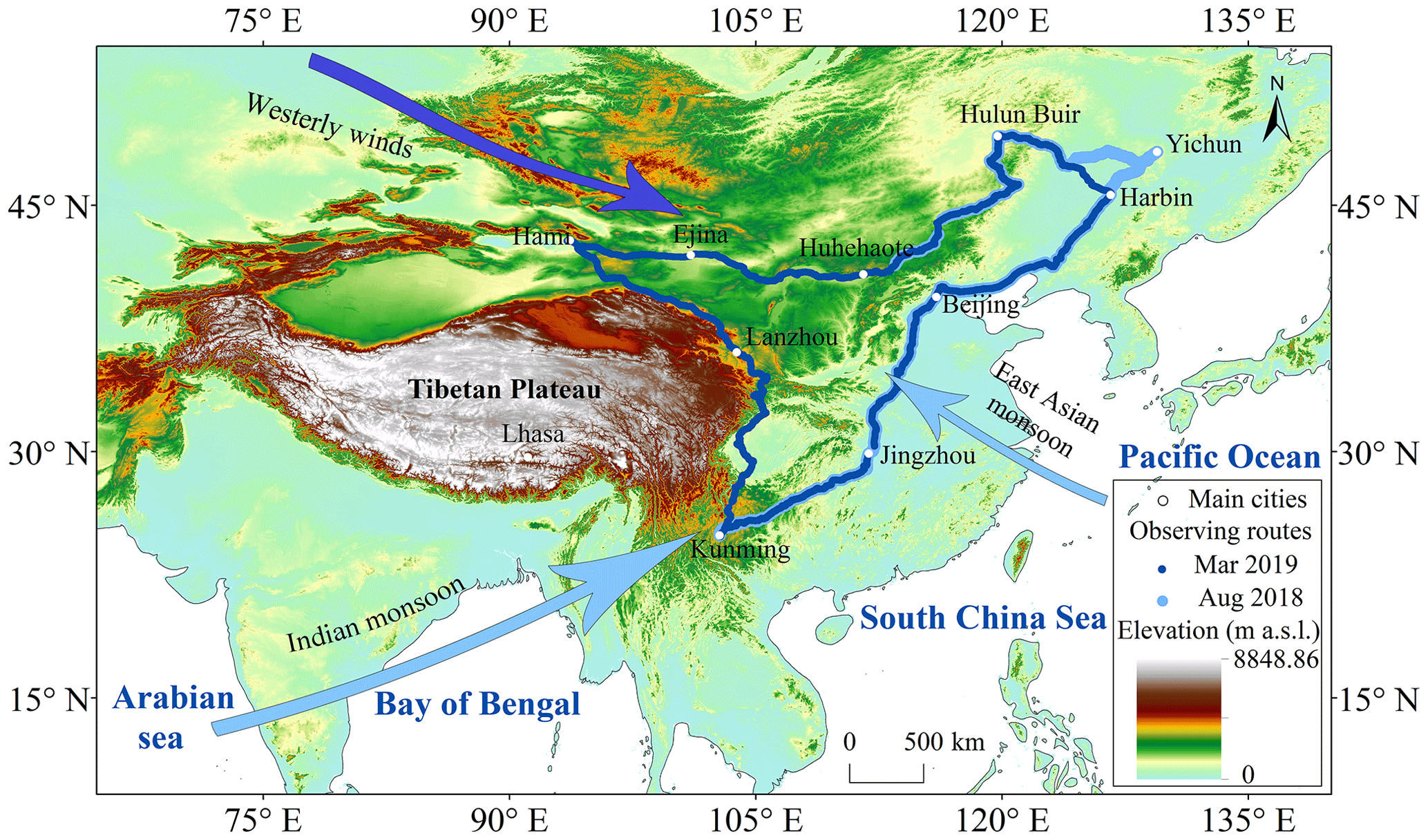
Figure 1Topographical map of China, showing survey routes and the main atmospheric circulation systems (arrows). Dark blue dots indicate the observation route for the 2019 pre-monsoon period, and light blue dots show the observation route for the 2018 monsoon period, with a slight deviation in the northeast.
2.2 Vapor isotope measurements
2.2.1 Isotopic definitions
Isotopic compositions of samples were reported as the relative deviations from the standard water (Vienna Standard Mean Ocean Water, VSMOW), using the δ notion (McKinney et al., 1950), where Rsample and RVSMOW are the isotopic ratios ( for δ18O and for δ2H) of the sample and of the VSMOW, respectively, as follows:
The second-order d-excess parameter is computed based on the commonly used definition (Dansgaard, 1964). The d-excess is usually interpreted as reflecting the moisture source and evaporation conditions (Jouzel et al., 1997), since the d-excess is more sensitive to non-equilibrium fractionation occurring than δ18O:
2.2.2 Instrument
We used a Picarro 2130i cavity ring-down spectroscopy (CRDS) water vapor isotope analyzer fixed on a vehicle to obtain large-scale in situ measurements of near-surface vapor isotopes along the route. The analyzer was powered by a lithium battery on the vehicle, enabling over 8 h operation with a full charge. Therefore, we only made measurements in daytime and recharged the battery at night. The ambient air inlet of the instrument was connected to the outside of the vehicle, which was 1.5 m a.g.l. (meters above ground level), with a waterproof cover to keep large liquid droplets from entering. A portable GPS unit was used to record position data along the route. The measured water vapor mixing ratio and the δ18O and δ2H were obtained with a temporal resolution of ∼ 1 s. The dataset present in this study had been averaged to a 10 min temporal resolution after calibration, with a horizontal footprint of about 15 km.
A standard delivery module (SDM) was used for the vapor isotope calibration during the surveys. The calibration protocols consist of humidity calibration (Sect. 2.2.3), standard water calibration (Sect. 2.2.4), and error estimation (Sect. 2.2.5), following the methods of Steen-Larsen et al. (2013).
2.2.3 Humidity-dependent isotope bias correction
The measured vapor isotopes are sensitive to air humidity (Liu et al., 2014; Galewsky et al., 2016), which varies substantially across our sampling route. The specific humidity measured by Picarro is very close to that measured by an independent sensor installed in the vehicle (Fig. 4). The correlation between the humidity measured by the Picarro and the independent sensor are over 0.99, the slopes are approximately 1, and the average deviations are less than 1 g kg−1 both during pre-monsoon and monsoon periods. We develop a humidity-dependent isotope bias correction by measuring a water standard at different water concentration settings using the SDM. We define a reference level of 20 000 ppm of vapor humidity for our analysis (Eq. 3), since the water vapor isotope measurement by Picarro is generally most accurate at this humidity. The calibrated vapor isotope with different air humidity would be as follows (Liu et al., 2014; Schmidt et al., 2010):
where δ_measured represents the measured vapor isotopes (the raw data), δ_humidity calibration denotes the calibrated vapor isotopes, f is the equation of δ as a function of humidity , and humidity is in ppm. For example, if we measured that f is ) by measuring standard water with different humidity, then the full equation for humidity-dependent isotope bias correction would be ).
We performed the humidity calibration before and after each campaign. In the calibration, the setting of humidity covered the actual range of humidity in the field. In the dry pre-monsoon period of 2019, the humidity was less than 5000 ppm along a large part of the route. In this case, we performed additional calibration tests with the humidity less than 5000 ppm after the field observations, to guarantee the accuracy of the calibration results. The humidity-dependence calibration function is considered constant throughout each campaign (which each lasted less than 24 d).
2.2.4 Measurement normalization
All measured vapor isotope values were calibrated to the VSMOW scale using two laboratory standard waters (δ18O = −10.33 ‰ and δ2H = −76.95 ‰, δ18O = −29.86 ‰ and δ2H = −222.84 ‰) covering the range of the expected ambient vapor values. We made the normalization test prior to the daily measurements (two humidity levels for each standard water). We adjusted the amount of the liquid standard injected everyday to keep the humidity of the standard waters consistent with the outside vapor measurements. Our calibration shows that no significant drift of the standard values were observed over time in the observation periods. For two standard waters, the standard deviation of standard measurements are 0.2 ‰ and 0.11 ‰ for δ18O, and 1.16 ‰ and 1.2 ‰ for δ2H during the pre-monsoon period of 2019. During the monsoon period of 2018, the standard deviation of standard measurements are 0.09 ‰ and 0.06 ‰ for δ18O and 0.6 ‰ and 0.33 ‰ for δ2H).
2.2.5 Error estimation
We estimate the uncertainty based on the error between the measured (after calibration) and true values of the two standards used during the campaigns. The estimated uncertainty is in the range of −0.05 to 0.17 for δ18O, 0.11 to 1.19 for δ2H, and −0.81 ‰ to 1.23 ‰ for d-excess during the pre-monsoon period of 2019, with the humidity ranges from 2000 to 29 000 ppm. During the monsoon period of 2018, the range of uncertainty is −0.10 ‰–0.55 ‰ for δ18O, −0.94 ‰–3.74 ‰ for δ2H, and −1.18 ‰–1.49 ‰ for d-excess, with the humidity ranges from 4000 to 34 000 ppm.
2.2.6 Data processing
A few isotope measurements with missing GPS information were excluded from the analysis. Since we want to focus on large-scale variations, we also removed the observations during rain or snow, to avoid situations where hydrometeor evaporation significantly influenced the observations (Tian et al., 2020). Such data represent only 0.03 % and 0.05 % of our observations, respectively (totally, 48 data during the pre-monsoon season and 59 data during the monsoon season). We observed several d-excess pulses with extremely low values, as low as −18.0 ‰, during the pre-monsoon period and −4.9 ‰ during the monsoon period. These low values are unusual in previous natural vapor isotope studies and occurred mostly when the measurement vehicle was entering or leaving cities and/or stuck in traffic jams, and they have a much lower intercept in the linear δ18O–δ2H relationship (Fig. S6). Previous studies on urban vapor isotopes (Gorski et al., 2015; Fiorella et al., 2018, 2019) showed that the vapor d-excess closely tracked changes in CO2 through inversion events and during the daily cycle dominated by patterns of human activity, and combustion-derived water vapor is characterized by a low d-excess value due to its unique source. We also find that the d-excess values are especially low when the vehicle was in cities in the afternoon. The values increased to normal during the night. This diurnal cycle is likely related to the emission intensity and atmospheric processes (Fiorella et al., 2018). Some of these d-excess anomalies are not excluded from being affected by the baseline effects emerging from rapid changes in concentrations of different trace gases (Johnson and Rella, 2017; Gralher et al., 2016). We therefore excluded these data (133 data points during the pre-monsoon period and 62 data points during the monsoon period represent 0.10 % and 0.06 % of our observations, respectively) in the discussion on the general spatial feature (except Fig. 4). Outside of towns, country sources, such as irrigation, farms, and power plants, cannot be completely ruled out. However, we expect their influence to be much smaller than large-scale spatial variations.
2.3 Meteorological observations
We fixed a portable weather station on the roof of the vehicle to obtain air temperature (T), dew-point temperature (Td), air pressure (Pres), and relative humidity (RH). All sensors were located near the ambient air intake. The specific humidity (q) of the near-surface air was calculated from Td and Pres. Meteorological data, GPS location data, and vapor isotope data were synchronized according to their measurement times. And all of them also had been averaged to a 10 min temporal resolution.
National Centers for Environmental Prediction/National Center for Atmospheric Research (NCEP/NCAR) 2.5∘ global reanalysis data are used to determine the large-scale factors influencing the spatial pattern of the vapor isotopes, including the surface T, q, U wind and V wind, and RH, which are available at https://psl.noaa.gov/data/gridded/data.ncep.reanalysis.surface.html (last access: March 2022). Some missing meteorological data (during the pre-monsoon period: q on 8 and 18 March 2019; during the monsoon period: T and q from 28 to 31 July 2018, and q on 5 August 2018) along the survey routes due to instrument failure are acquired from the NCEP/NCAR reanalysis data. To match the vapor isotope data along the route, we linearly interpolate the NCEP/NCAR data to the location and time of each measurement. The interpolated T and q from NCEP/NCAR are highly correlated with our measurement, as shown in Fig. 4h and j. The 1∘ precipitation amount (P) from the Global Precipitation Climatology Project (GPCP) is used (https://www.ncei.noaa.gov/data/global-precipitation-climatology-project-gpcp-daily/access/, last access: March 2022). When comparing the time series of GPCP data with our observed isotopes, we linearly interpolate the daily GPCP data to the location of each observation location (P daily). We also used the average of the GPCP precipitation over the entire observation period of about 1 month for each observation location (P mean). The 2.5∘ outgoing longwave radiation (OLR) data can be obtained from NOAA (http://www.esrl.noaa.gov/psd/data/gridded/data.interp_OLR.html, last access: March 2022).
2.4 Back-trajectory calculation and categorizing regions based on air mass origin
The vapor isotope composition is a combined result of moisture source (Tian et al., 2007; Araguás-Araguás et al., 1998), condensation, and mixing processes along the moisture transport route (Galewsky et al., 2016). To interpret the observed spatial–temporal distribution of vapor isotopes, we start with a diagnosis of the geographical origin of the air masses and then analyze the processes along the back trajectories.
To trace the geographical origin of the air masses, the HYSPLIT-compatible meteorological dataset of the global data assimilation system (GDAS) is used (available at ftp://arlftp.arlhq.noaa.gov/pub/archives/gdas1/, last access: March 2022). We select the driving locations every 2 h as starting points for the backward trajectories and make 10 d back trajectories from 1000 m a.g.l. using the Hybrid Single Particle Lagrangian Integrated Trajectory model 4 (HYSPLIT4) (Draxler and Hess, 1998). This is representative of the water vapor near the ground (Guo et al., 2017; Bershaw et al., 2012), since most water vapor in the atmosphere is within 0–2 km a.g.l. (Wallace and Hobbs, 2006). The T, q, P, and RH along the back trajectories are also interpolated by the HYSPLIT4 model (Fig. 2).
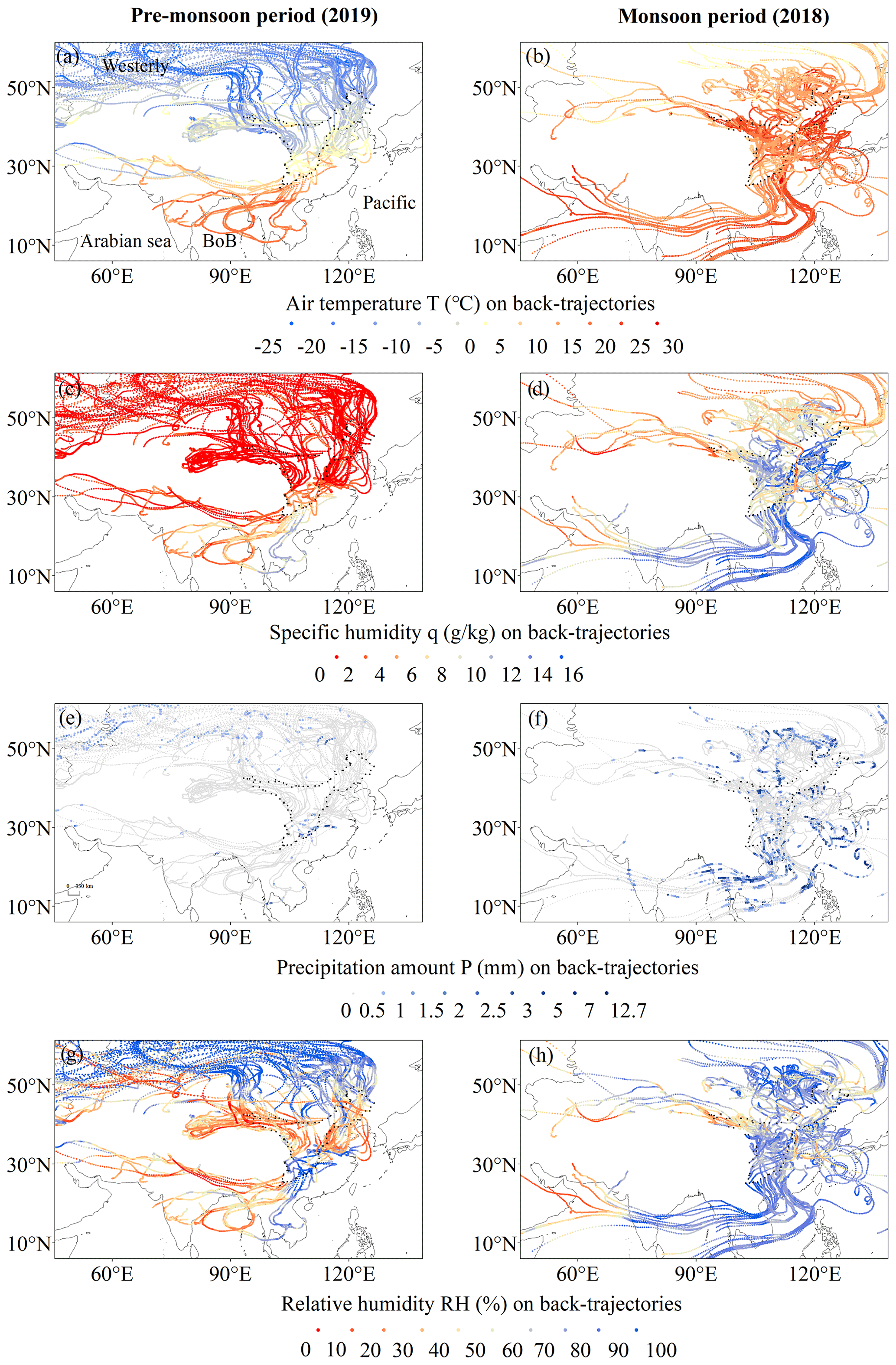
Figure 2Meteorological conditions simulated by the HYSPLIT4 model along the 10 d air back trajectories for the on-route sampling positions during the two surveys: (a, b) air temperature T (∘C), (c, d) specific humidity q (g kg−1), (e, f) precipitation amount P (mm), and (g, h) relative humidity RH (%). The left panel is for the pre-monsoon period, and the right is for the monsoon period. The driving locations and time every 2 h are used as starting points. Note: BoB is the abbreviation for the Bay of Bengal.
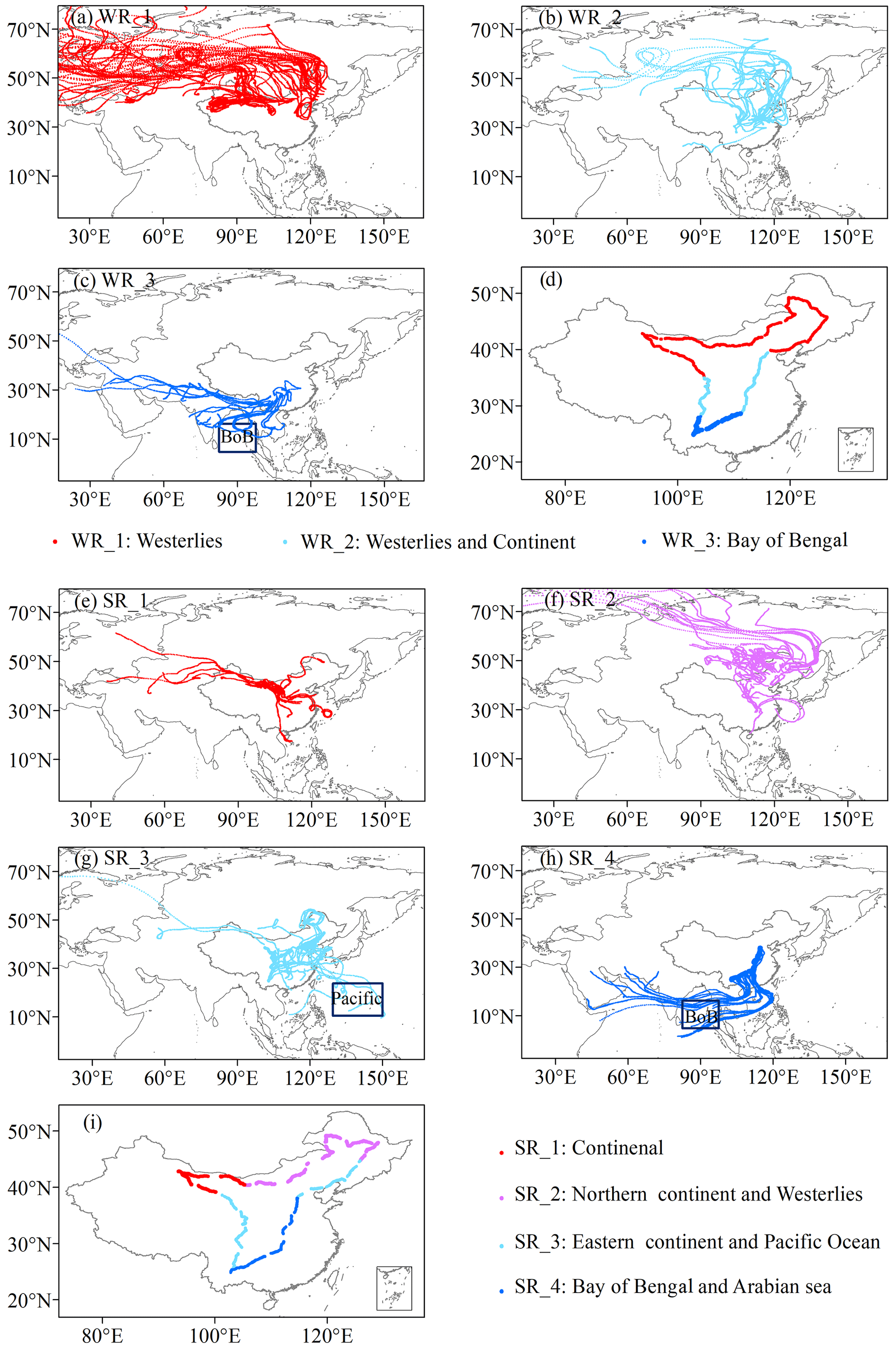
Figure 3The backward trajectory results (a, b, and c for the pre-monsoon period, and e, f, g, and h for the monsoon period) and the dividing of the study zones based on geographical origin of the air masses (d for the pre-monsoon period and i for the monsoon period). Note: BoB is the abbreviation for the Bay of Bengal.
Based on the tracing results from HYSPLIT4 model, we speculate on the potential water vapor sources (Fig. 3 and Table 1):
During the pre-monsoon period, we categorize our domain into three regions (Table 1) as follows:
-
In northern China (WR_1), the air is mainly advected by the westerlies.
-
In central China (WR_2), the air also comes from the westerlies but with a slower wind speed (as shown by the shorter trajectories in 10 d), suggesting the potential for greater interaction with the land surface and more continental recycling as the moisture source.
-
In southern China (WR_3), trajectories come from the southwest and South with marine moisture sources from the Bay of Bengal (BoB).
During the monsoon period, we categorize our domain into four regions (Table 1) as follows:
-
In northwestern China (SR_1), most air masses also spend considerable time over the continent, suggesting some of the vapor can be recycled by continental recycling.
-
In northeastern China (SR_2), trajectories mainly come from the North and though the westerlies.
-
In central China (SR_3), both in its eastern (from Beijing to Harbin) and western part, trajectories mainly come from the East. This suggests that vapor mainly comes from the Pacific Ocean or from continental recycling over eastern and central China.
-
In southeastern China (SR_4), trajectories come from the South, suggesting marine moisture sources from the Arabian Sea and the BoB.
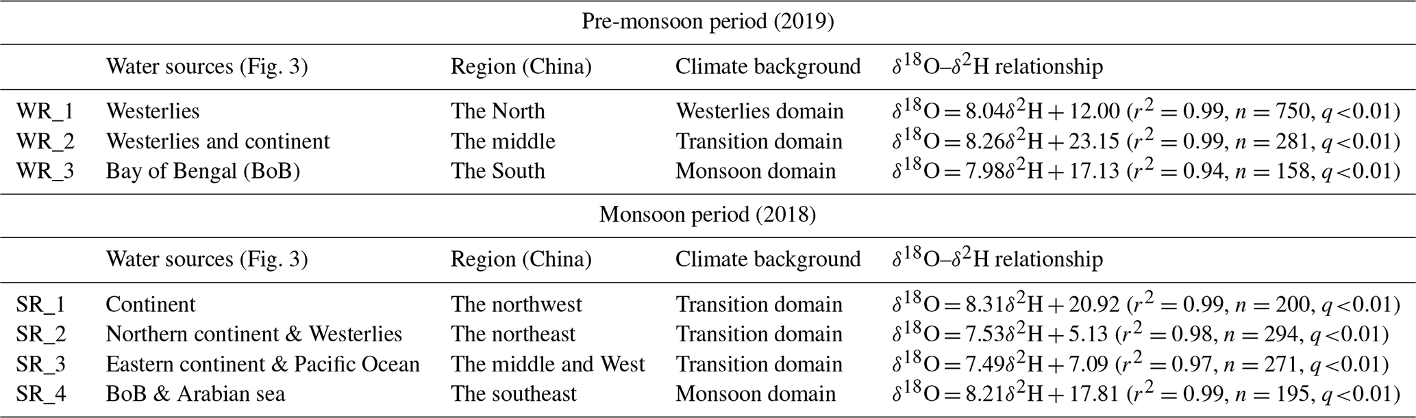
Table 1The dividing of the study zones based on moisture sources and corresponding vapor δ18O–δ2H relationship.
2.5 General circulation model simulation and satellite measurements
To disentangle the spatial and synoptic influences, we use surface layer variables from an isotope-enabled general circulation model (Iso-GSM) simulations (Yoshimura and Kanamitsu, 2009) at 1.915∘ × 1.875∘ and the lowest level (the altitude is about 2950 m) isotope retrievals from satellite infrared atmospheric sounding interferometer (IASI) at 1∘ × 1∘. For both datasets, we use the outputs corresponding to the observation location and the observation date (daily outputs) and the multiyear monthly mean outputs (March monthly for the pre-monsoon period and August monthly for the monsoon period) for each observation location from 2015 to 2020. When interpolating daily/multiyear monthly outputs, we select the nearest grid point for a given latitude and longitude of each measurement. For Iso-GSM simulations, because of the coarse resolution of the model, there is a difference between the altitude observed along the sampling route and that of the nearest grid point. Therefore, we correct the outputs of Iso-GSM for this altitude difference (the method is given in the Supplement under “III. Supplementary Text”). Since the satellite only retrieves δ2H, we just use δ2H outputs of Iso-GSM and satellite to quantify the relative contributions of seasonal mean and synoptic-scale variations (Sect. 3.3). Other than that, our discussion focuses on δ18O and d-excess. The variations of δ2H are consistent with those of δ18O. We also interpret the biases in Iso-GSM after we understand the factors influencing the spatial and seasonal variation of vapor isotopes (Sect. 4.6).
2.6 Method to decompose the observed daily variations
The temporal variations observed along the route for a given period represent a mixture of synoptic-scale perturbations and of seasonal mean spatial distribution as follows:
The first term represents the contribution of seasonal mean spatial variations, whereas the second term represents the contribution of synoptic-scale variations. Since these relative contributions are unknown, we use outputs from Iso-GSM and IASI. The daily variations of δ2H simulated by Iso-GSM also represent a mixture of synoptic-scale perturbations and seasonal mean spatial distribution, but with some errors relative to reality:
where δ2H_daily_Iso-GSM is the daily outputs of δ2H for each location, δ2H_seaso_Iso-GSM is the multiyear monthly outputs of δ2H for each location, and δ2H_synoptic_Iso-GSM= δ2H_daily_Iso-GSM−δ2H_seaso_Iso-GSM; each of these terms are affected by errors relative to observations as follows:
where ∈_seaso and ∈_synoptic are the errors on δ2H_seao_Iso-GSM and δ2H_synoptic_Iso-GSM relative to reality, respectively, and ∈ is the sum of ∈_seaso and ∈_synoptic.
Correspondingly,
These individual error components ∈_seaso and ∈_synoptic are unknown, but we know the sum of them (∈), i.e., the difference between daily outputs and observations. For the decomposition, we made two extreme assumptions to estimate upper and lower bounds on the contribution values as follows:
-
If we assume that the error is purely synoptic, i.e., , and ∈_seaso = 0, then
To evaluate the contribution of these two terms, we calculate the slopes of δ2H_daily as a function of δ2H_seaso_Iso-GSM (a_seaso) and of δ2H_daily−δ2H_seaso_Iso-GSM (a_synoptic). The relative contributions of spatial and synoptic variations correspond to a_seaso and a_synoptic, respectively. This will be the upper bound for the contribution of synoptic-scale variations, since some of the systematic errors of Iso-GSM will be included in the synoptic component. This is equivalent to using the seasonal mean of Iso-GSM and the raw time series of observations.
-
If we assume that the error is purely seasonal mean, i.e., and ∈_synoptic = 0, then
To evaluate the contribution of these two terms, we calculate the slopes of δ2H_daily_Iso-GSM as a function of δ2H (a_seaso) and of δ2H_daily−(δ2H (a_synoptic). This will be the lower bound for the contribution of synoptic-scale variations, since we expect Iso-GSM to underestimate the synoptic variations.
The same analysis is also performed for δ2H retrieved from IASI and the Iso-GSM simulation q (Table 2) and reanalysis q (Table 3).
3.1 Raw time series
Our survey of the vapor isotopes yields two snapshots of the isotopic distribution along the route (Figs. 4 and 5). Figure 4 shows the variations of observed 10 min averaged surface vapor δ18O and d-excess along the survey route across China during the pre-monsoon and monsoon campaigns. The figure also shows the concurrent meteorological data from the weather station installed on the vehicle, and the water vapor content recorded by the Picarro water vapor isotope analyzer as a comparison. We extract daily precipitation amount (P daily) and average precipitation amount over the entire observation period of about 1 month for each observation location (P mean) (mm d−1) from GPCP. The vapor δ18O shows high magnitude variations in both seasons. A general decreasing–increasing trend overlapped with short-term fluctuations is observed during the pre-monsoon period, whereas no general trend but frequent fluctuations characterized the monsoon period. The δ18O range is much larger during the pre-monsoon period (varying between −44 ‰ and −8 ‰) than during the monsoon period (from −11 ‰ to −23 ‰). Most measured vapor d-excess values range from 5 ‰ to 25 ‰ during the pre-monsoon period and from 10 ‰ to 22 ‰ during the monsoon period.
Comparison with the concurrently observed meteorological data shows a robust air temperature (T) dependence of the vapor δ18O variations. In particular, the general trend of δ18O is roughly consistent with T variation during the pre-monsoon period (Fig. 4a and g). During the pre-monsoon period, humidity (Fig. 4e and i), P mean (Fig. 4k), and vapor δ18O (Fig. 4a) are much higher in southwestern China (at the beginning and end of the campaign) than in any other regions. Humidity, q, and P mean also vary consistently throughout the route during the monsoon period (Fig. 4f, j, and l). Synoptic effects on the observed vapor isotopes are discussed in detail in Sect. 4.3 and 4.6.

Figure 4Measured vapor isotopic compositions and concurrent meteorological conditions along the survey routes during the pre-monsoon period (the left panel) and monsoon period (the right panel). (a, b) Vapor δ18O (‰); (c, d) vapor d-excess (‰); (e, f) specific humidity q (g kg−1) measured by sensor (in green), measured by Picarro (in blue), and linearly interpolated from NCAR reanalysis (in gray); (g, h) air temperature T (∘C) measured by Picarro (in orange) and linearly interpolated from NCAR reanalysis (in gray); and (i, j) the daily precipitation amount P daily (in green, mm d−1) and average precipitation amount over the entire observation period of about 1 month for each observation location P mean (in blue, mm d−1) extracted from GPCP. Note that the vertical gray lines space the observations for 1 d.
3.2 Spatial variations
The spatial distribution of the observed vapor δ18O and d-excess during the two surveys in different seasons are presented in Figure 5. During the pre-monsoon period, we find a South–North gradient of vapor δ18O (Fig. 5a). The vapor δ18O ranges from −8 ‰ to −16 ‰ in southern China to as low as −24 ‰ to −44 ‰ in the North. A roughly similar spatial pattern is observed for the vapor d-excess during the pre-monsoon period (Fig. 5c). The d-excess value ranges from 10 ‰ to 30 ‰ in southern China and from −10 ‰ to +20 ‰ (most observations with values from 5 ‰ to +20 ‰) in northern China. In previous studies, a higher precipitation d-excess during the pre-monsoon period was also observed in the Asian monsoon region owing to the lower relative humidity (RH) at the surface in the moisture source region (Tian et al., 2007; Jouzel et al., 1997). The same reason probably explains the higher vapor d-excess in southern China observed here. Alternatively, the high d-excess in South China could also result from the moisture flow from the Indian/Pacific Ocean, or from the deeper convective mixed layer in South China compared to North China. The lower d-excess values (as low as −10 ‰ to 10 ‰) in northern China (between 38 and 51∘ N) have rarely been reported in earlier studies. The spatial distribution of the observed vapor d-excess could reflect the general latitudinal gradient of d-excess observed at the global scale, with a strong poleward decrease in midlatitudes (between around 20 to 60∘), which was found in previous studies on the large-scale distribution of d-excess in vapor (Thurnherr et al., 2020; Benetti et al., 2017) and precipitation (Risi et al., 2013a; Terzer-Wassmuth et al., 2021; Pfahl and Sodemann, 2014; Bowen and Revenaugh, 2003), based on both observations and modeling. During the monsoon period, the lowest values of vapor δ18O are found in southwestern and northeastern China, with a range of −23 ‰ to −19 ‰ (Fig. 5b). Higher vapor δ18O values up to −11 ‰ are found in central China. The vapor d-excess values (Fig. 5d) in western and northwestern China (91–109∘ E, 24–43∘ N) are roughly between 16 ‰ and 22 ‰, higher than in eastern China (mostly between 0 ‰ and 16 ‰).
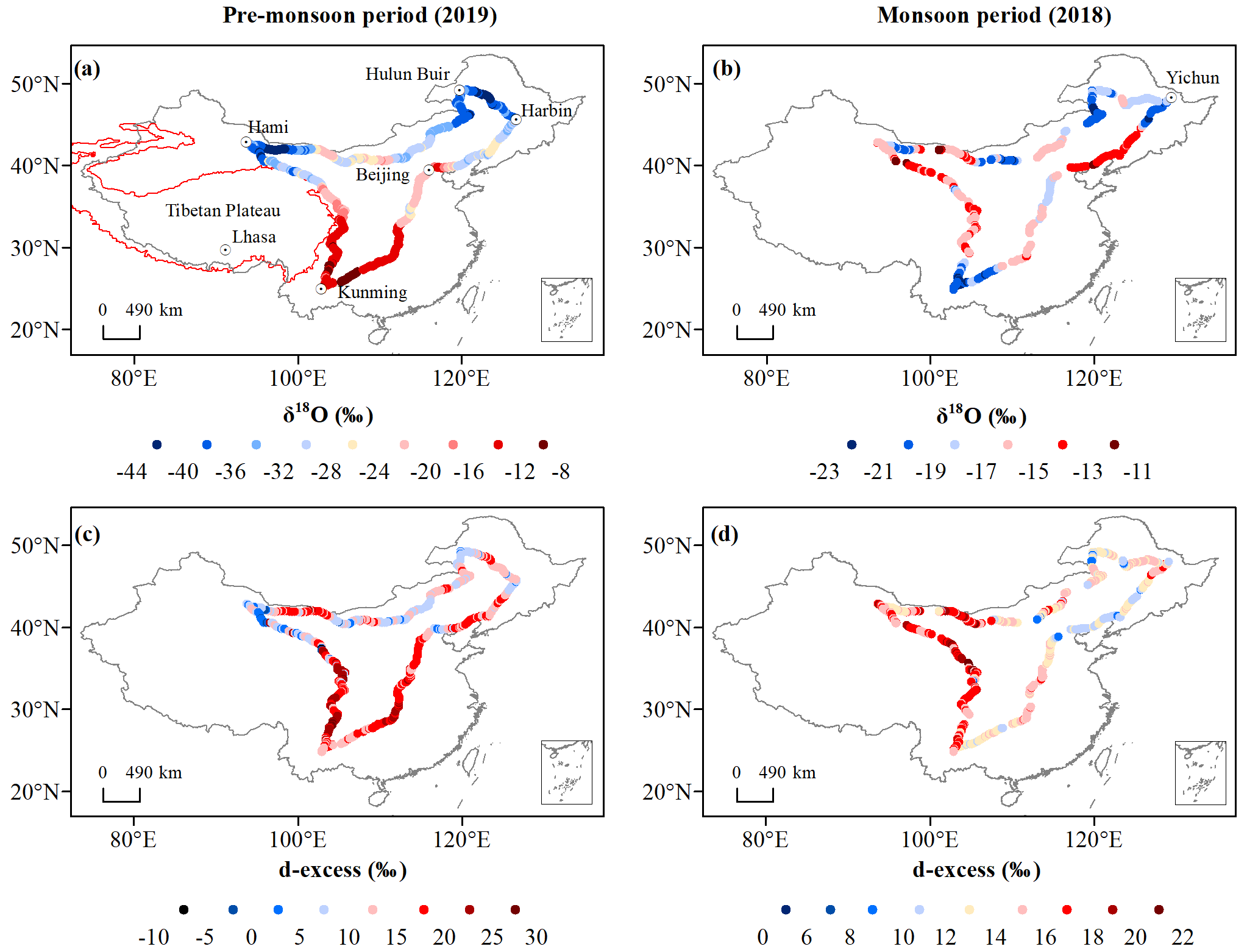
Figure 5Spatial distribution of vapor δ18O (a, b) and d-excess (c, d) during the pre-monsoon period (a, c) and the monsoon period (b, d).
We do not know whether these apparent spatial variations represent the seasonal mean or whether it is mainly affected by synoptic perturbations. We therefore use Iso-GSM simulation results and IASI satellite measurements to quantify the relative contributions of seasonal mean and synoptic perturbations in Sect. 3.3.
3.3 Disentangling seasonal mean and synoptic variations
Figure 6 shows the comparison of the measured vapor δ2H, simulated δ2H from Iso-GSM, and the δ2H retrieved from IASI. Iso-GSM captures the variations in observed vapor δ2H well during the pre-monsoon period, with a correlation coefficient of r=0.84 (p<0.01) (Table S3). The daily simulation results during the monsoon period are roughly in the range of observations, but detailed fluctuations are not well captured, with r=0.24 (p>0.05) (Table S3). The largest differences occur in the SR_1 zone. IASI captures variations better than Iso-GSM during the monsoon period, with r=0.42 (p>0.05). IASI observes over a broad range of altitudes above the ground level, so we expect lower δ2H in IASI relative to ground-surface observations, but the variations of vapor isotopes are vertically coherent (Fig. 6). The systematic differences between IASI and ground-level observations do not impact the slope of the correlation, and thus does not impact the contribution estimation.
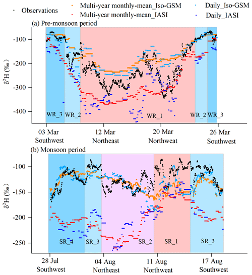
Figure 6Comparison of observed vapor δ2H (observations) with outputs of isotope-enabled general circulation model Iso-GSM and satellite IASI during the pre-monsoon period (a) and monsoon period (b). The results in this graph are from the daily and multiyear monthly outputs for the sampling locations.
The multiyear monthly means of δ2H are smoother but similar to those for the daily outputs both from Iso-GSM and IASI (Fig. 6). Using the method in Sect. 2.6, taking into account the error, we calculate the relative contribution ranges of the seasonal mean and synoptic scale on our observed variations using q and δ2H from Iso-GSM simulations, q from NCEP/NCAR reanalysis, and δ2H from IASI.
Table 2The relative contribution (in fraction) of spatial variations for a given season (a_seaso) and of synoptic-scale variations (a_synoptic) to the daily variations of q and δ2H simulated by Iso-GSM and retrievals from IASI. We checked that the sum of a_seaso and a_synoptic is always 1. The two values indicate the lower and upper bounds as calculated from Eqs. (8) and (9).
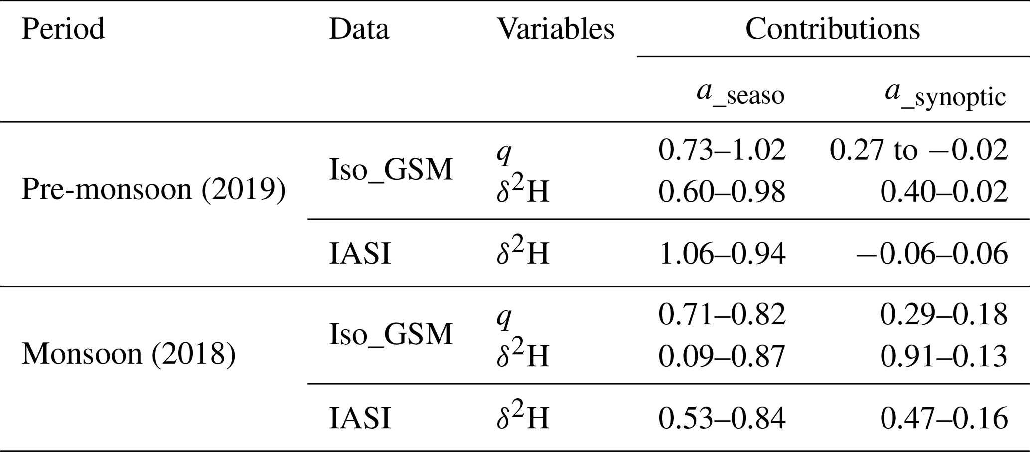
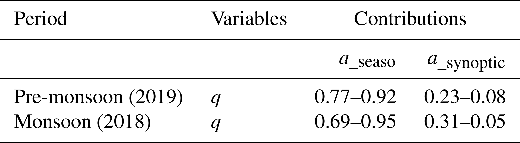
During the pre-monsoon period, based on both the Iso-GSM simulation and NCEP/NCAR reanalysis, we can find that the seasonal mean contribution to the measured q is higher than the synoptic-scale contribution: a_seaso is 73 %–102 % from Iso-GSM and 77 %–92 % from reanalysis, whereas a_synoptic is 27 % to −2 % from Iso-GSM and 23 %–8 % from reanalysis (Tables 2 and 3). The relative contribution of seasonal mean spatial variations to the total measured variations in δ2H (60 %–98 %) is also higher than that of synoptic-scale variations (40 %–2 %). This suggests that the observed variability in q and δ2H is mainly due to spatial variability and marginally due to synoptic-scale variability. During the monsoon, seasonal mean spatial variations are also the main contributions to the observed variations of q (a_seaso is 71 %–82 % from Iso-GSM and 69 %–95 % from reanalysis, whereas a_synoptic is 29 %–18 % from Iso-GSM and 31 %–5 % from reanalysis). Since Iso-GSM does not capture daily variations of δ2H very well during the monsoon period, the relative contribution has a large threshold range (a_seaso is 9 %–87 %, a_synoptic is 91 %–13 %) after accounting for the errors. Therefore, we can not conclude the dominant contribution on δ2H from Iso-GSM outputs. IASI, which has a higher correlation with observations, provides an more credible range of a_seaso, about 53 %–84 %, and a_synoptic is 47 %–16 %. These suggest that during the monsoon period, the synoptic contribution can be significant but not dominant. Having understood the factors influencing the spatial and seasonal variation of vapor isotopes in Sect. 4, we will be able to better understand the reasons for the inconsistent performance of Iso-GSM during the pre-monsoon and monsoon periods (in Sect. 4.6).
3.4 Seasonal variations
During the monsoon season, synoptic-scale and intra-seasonal variations contribute significantly to the apparent spatial patterns. However, since these variations are not dominant and have a smaller amplitude than seasonal differences, the comparison of the two snapshots do provide a representative picture of the climatological seasonal difference.
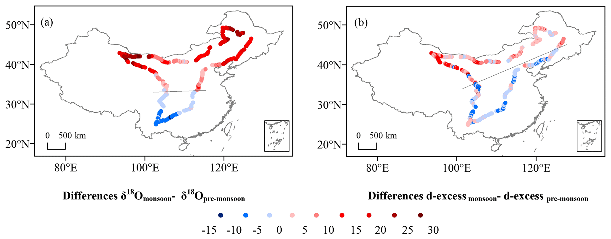
Figure 7Spatial distribution of the isotope differences (δ18Omonsoon−δ18Opre-monsoon (a) and d-excessmonsoon− d-excesspre-monsoon (b)) for the observation locations. The solid black lines separate the areas of positive and negative values of the differences.
The climate in China features strong seasonality, and it is captured in the snapshots of vapor isotopes (Fig. 7). Since the observation routes of the two surveys are almost identical, we make a seasonal comparison of the observed vapor isotopes during the two surveys. The lines are drawn to distinguish between positive and negative values of seasonal isotopic differences. The seasonal differences δ18Omonsoon−δ18Opre-monsoon (Fig. 7a) show opposite signs in northern and southern China. In northern China, water vapor δ18O values are higher during the monsoon period than during the pre-monsoon period, while the opposite is true in southern China. The boundary is located around 35∘ N. The largest seasonal contrasts occur in southwest, northwest, and northeast China, with seasonal δ18O differences of −15 ‰, 30 ‰, and 30 ‰, respectively.
We also find a spatial pattern of vapor d-excess seasonality (Fig. 7b). The line separating the areas of positive and negative values of the d-excessmonsoon− d-excesspre-monsoon differences coincides with the 120 mm mean precipitation line (Fig. S2f). In southeastern China, the water vapor d-excess is lower during the monsoon period than during the pre-monsoon period. The pattern of seasonal water vapor d-excess in northwestern China is the opposite. The two boundary lines separating the seasonal variations of δ18O and d-excess do not overlap, suggesting different controls on water vapor δ18O and d-excess.
To interpret the spatial and seasonal variations observed both across China and in each region defined in Sect. 2.4, we investigate q–δ diagrams (Sect. 4.1), δ18O–δ2H relationships (Sect. 4.2), relationships with meteorological conditions at the local and regional scale (Sect. 4.3 and 4.4), the impact of air mass origin (Sect. 4.5), and synoptic events (Sect. 4.6).
4.1 q–δ diagrams
The progressive condensation of water vapor from an air parcel from the source region to the sampling site and the subsequent removal of condensate results in a gradual reduction of humidity and vapor isotope ratios. This relationship can be visualized in a q–δ diagram, which has been used in many studies of the vapor isotopic composition (Noone, 2012; Galewsky et al., 2016). Observations along the Rayleigh distillation line indicate progressive dehydration by condensation. Observations above the Rayleigh line indicate either mixing between air masses of contrasting humidity (Galewsky and Hurley, 2010) or evapotranspiration (Galewsky et al., 2011; Samuels-Crow et al., 2015; Noone, 2012; Worden et al., 2007). Observations below the Rayleigh line, even when considering the most depleted initial vapor conditions (light blue Rayleigh curve in Fig. 8b), indicate the influence of rain evaporation from depleted precipitation (Noone, 2012; Worden et al., 2007). Figure 8 shows the observed vapor q–δ2H for different regions during the pre-monsoon (a) and monsoon (b) period. This figure will be interpreted in the light of meteorological variables along back trajectories (Fig. 2).
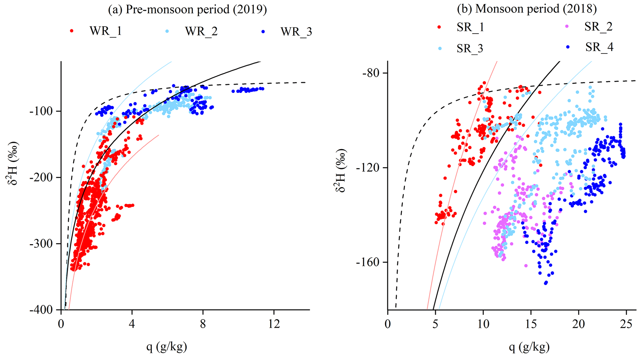
Figure 8Scatterplot of observed vapor δ2H (‰) versus specific humidity q (g kg−1) during the pre-monsoon period (a) and monsoon (b) period. The solid black curves show the Rayleigh distillation line calculated for the initial conditions of δ2H ‰ and T=15 ∘C during the pre-monsoon period and δ2H ‰ and T=25 ∘C during the monsoon period. The mixing lines (dashed black curves) are calculated using a dry endmember with q=0.2 g kg−1 and δ2H ‰ and air parcels for the corresponding Rayleigh curve as a wet endmember. The solid colored curves show the uncertainty range of the Rayleigh curve, calculated for different initial conditions of key moisture source regions: during March 2019, light red and light blue Rayleigh curves are calculated for key moisture source regions of westerlies (δ2H ‰, T=5 ∘C) and BoB (δ2H ‰, T=26.46 ∘C) separately in (a); during July–August 2018, light red and light blue Rayleigh curves are calculated for key moisture source regions of westerlies (δ2H ‰, T=6.16 ∘C) and BoB (δ2H ‰, T=27.69 ∘C) separately in (b). These initial δ2H are derived from Iso-GSM, and the initial temperature and RH are derived from NCAR/NCEP 2.5∘ global reanalysis data.
During the pre-monsoon period, most q–δ2H measurements are located surrounding or overlapping the Rayleigh curve (the solid black curve in Fig. 8a). Therefore, the observed spatial pattern can mostly be explained by the gradual depletion of vapor isotopes by condensation. The data for the three moisture sources are distributed in different positions of the Rayleigh curve, and they relate to different moisture origins or different original vapor isotope values. This is confirmed by the back-trajectory analysis: the westerlies bring cold and dry air to northern China (WR_1, Figs. 3a, 2a and c), consistent with the vapor further along the Rayleigh distillation, and are thus very depleted (Fig. 5a). The observations in the WR_1 region (Fig. 3c) are closer to the q–δ2H Rayleigh distillation curve calculated for the key moisture source regions of westerlies, providing further evidence of the influence of water vapor source on vapor isotopes. The relatively high T and q along the ocean-sourced air trajectory reaching southern China (WR_3, Figs. 3c, 2a and c) is consistent with an early Rayleigh distillation phase during moisture transport and thus higher water vapor δ18O in southern China (Fig. 5a). Some observations in the WR_3 region (Fig. 3c) are located below the q–δ2H Rayleigh distillation curve, indicating the influence of rain evaporation (Noone, 2012; Worden et al., 2007). This is consistent with the fact that air originates from the BoB, where deep convection begins to be active, and thus rain evaporation become a source of water vapor.
During the monsoon period, we find a scattered relationship in the q–δ2H diagram for different regions, implying different moisture sources and/or water recycling patterns during moisture transport. Data measured in the SR_1 region (Fig. 3i) fall above the Rayleigh distillation line (solid black curve in Fig. 8b), likely due to the presence of moisture originating from continental recycling. A larger number of q–δ2H measurements (most of the measurements from the SR_2, SR_3, and SR_4 regions, Fig. 3i) are located below the Rayleigh curve, indicating moisture originating from the evaporation of raindrops within and below convective systems (Noone, 2012; Worden et al., 2007). In SR_3 and SR_4 regions, this is consistent with the high precipitation rate along southerly and easterly back trajectories (Fig. 2f). The convection is active over the Bay of Bengal, Pacific Ocean, and southeastern Asia, as shown by the low OLR (<240 W m−2) in these regions (Fig. S3) (Wang and Xu, 1997). Therefore, a significant fraction of the water vapor originates from the evaporation of raindrops in convective systems. These results support recent studies showing that convective activity depleted the vapor during transport by the Indian and East Asian monsoon flow (Cai et al., 2018; He et al., 2015; Gao et al., 2013). In the SR_2 region, the relatively low water vapor δ18O, below the Rayleigh curve, is also probably associated with the evaporation of raindrops under deep convective systems. This is confirmed by the high precipitation rates along northerly back trajectories (Fig. 2f), reflecting summer continental convection.
In northern China, q–δ diagrams show stronger distillation during the pre-monsoon period (red dots in Fig. 8a). This suggests a “temperature-dominated” control. Very low regional T during the pre-monsoon period (Figs. S2a and 2a) are associated with low saturation vapor pressures and enhanced distillation, producing lower vapor δ18O. The T in summer is higher (Figs. S2b and 2b), allowing for higher vapor δ18O (red dots in Fig. 8b). The δ18Omonsoon−δ18Opre-monsoon values in this region are therefore positive (Fig. 7a). In the South, q–δ diagrams suggest the stronger influence of rain evaporation during the monsoon period. Higher precipitation amounts significantly reduce δ18O in the South (Fig. 2f), even though T was higher during the monsoon period than in pre-monsoon. This suggests a precipitation-dominated control in this region, explaining the negative values of δ18Omonsoon−δ18Opre-monsoon. This seasonal pattern in δ18O is consistent with the results in precipitation isotopes (Araguás-Araguás et al., 1998; Wang and Wang, 2001). The boundary line separating the seasonal variations of δ18O is also consistent with a previous study on the seasonal difference in vapor δ2H retrieved by the Technology Experiment Satellite (TES) and Greenhouse Gases Observing Satellite (GOSAT; Shi et al., 2020).
4.2 The δ18O–δ2H relationship
The δ18O–δ2H relationship is usually applied to diagnose the moisture source and water cycling processes related to evaporation. Figure 9 and Table 1 show the δ18O–δ2H relationship for different regions in the two seasons. We also plot the East Asian meteoric water line (EAMWL) for a reference. Vapor δ18O–δ2H is usually located above the meteoric water line owing to the liquid water and vapor fractionation.
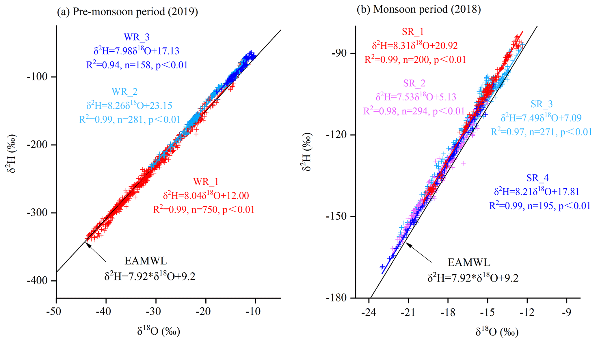
Figure 9Regional patterns of vapor δ18O–δ2H relation during pre-monsoon period (a) and monsoon (b) period, compared with the East Asia meteoric water line (EAMWL) (Araguás-Araguás et al., 1998).
During the pre-monsoon period (Fig. 9a), the data in northern China (WR_1, Fig. 3a) are located at the lower left area in the δ18O–δ2H graph, with a similar slope and intercept as EAMWL (δ2H = 8.04 δ18O + 12.00). This corresponds to air brought by the westerlies and following Rayleigh distillation. The linear relationship for the vapor in middle China (WR_2, Fig. 3b) has the steepest slope and highest intercept (δ2H = 8.26δ18O + 23.15). These properties are associated with a high d-excess, consistent with strong continental recycling by evapotranspiration (Aemisegger et al., 2014), as continental recycling is known to enrich the water vapor (Salati et al., 1979) and is associated with high d-excess (Gat and Matsui, 1991; Winnick et al., 2014). The high intercept is further consistent with a correlation between δ18O and d-excess, which can typically result from continental recycling (Putman et al., 2019). The data for vapor originating from the BoB (WR_3, Fig. 3c) are located to the upper right of the EAMWL. Their regression correlation shows similar features (δ2H = 7.98 δ18O + 17.13) to that of the monsoon season (with a slope of 8.21 and an intercept of 17.81). We find similar atmospheric conditions in the BoB (with the region marked as the rectangle in Fig. 3c and h) during the two observation periods, with T=26 ∘C and RH = 76 % during the pre-monsoon period and T=28 ∘C and RH = 78 % during the monsoon period, suggesting that the BoB source may have similar signals on vapor δ18O and δ2H in both seasons. These observed vapor δ18O–δ2H patterns are consistent with the back-trajectory results indicating that the westerlies persist in northern China during the pre-monsoon period while moisture from the BoB has already reached southern China.
During the monsoon period (Fig. 9b), the data in northwestern China (SR_1, Fig. 3e) with continental moisture sources are located in the upper right of the graph but above the EAMWL, with the steepest slope and highest intercept for the linear δ18O–δ2H relationship (δ2H = 8.31δ18O + 20.92). In contrast, the observations in southeastern China with BoB sources (SR_4, Fig. 3h) are located in the lower left of the graph, with a relatively lower intercept (δ2H = 8.21δ18O + 17.81). This is the opposite pattern compared to the pre-monsoon season. The observations from the SR_3 region (Fig. 3g) also have a low slope and low intercept (δ2H = 7.49 δ18O + 7.09). This is consistent with the oceanic moisture from the Pacific Ocean. Also, these δ18O–δ2H data are located in the upper right of the graph with a more scattered relation (with the lowest correlation coefficient), suggesting more diverse moisture sources. This is consistent with the mixing of water vapor from continental recycling and the Pacific Ocean (Fig. 3g). The observations in northeastern China (SR_2, Fig. 3f) are located at the lower left of the graph, suggesting the influence of condensation along trajectories in northern Asia (Fig. 2f). Compared to the SR_3 and SR_4 regions, the slope and intercept of the observations in SR_2 region are lower (δ2H = 7.53δ18O + 5.13), reflecting different origins of moisture.
4.3 Relationship with local meteorological variables
Here we analyze the relationship between vapor δ18O, d-excess, and local meteorological parameters for all observations and separately for the different regions (Fig. 10 and Table S1).
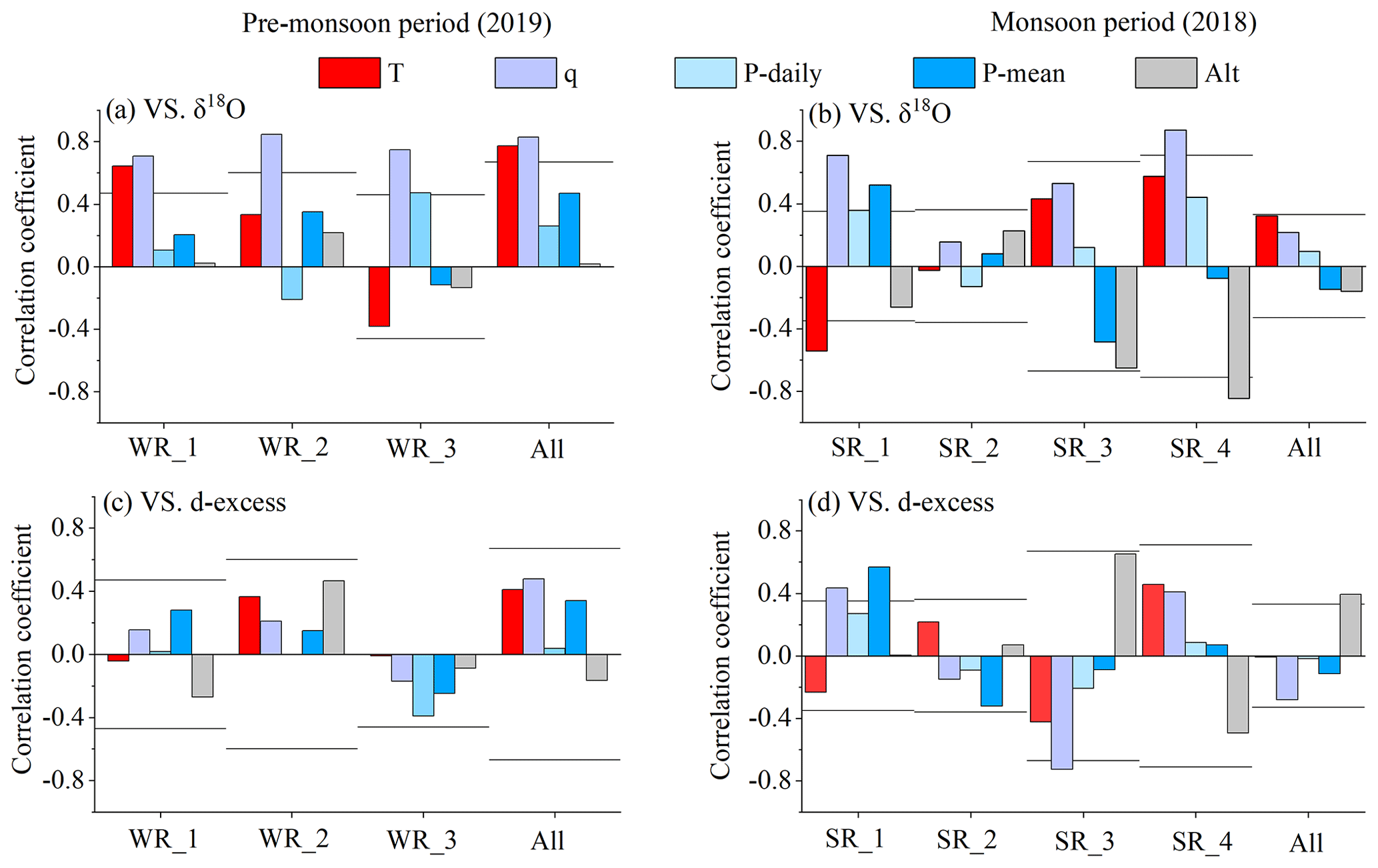
Figure 10Regional patterns of the correlation between δ18O (a, b), d-excess, (c, d) and various local factors (temperature (T), specific humidity (q), daily precipitation amount (P daily), and average precipitation amount over the entire observation period for each observation location (P mean), and altitude (Alt)). (a, c) is for the pre-monsoon period and (b, d) is for the monsoon period. Horizontal lines indicate the correlation threshold for statistical significance (p<0.05), considered the degree of freedom.
We have taken particular care to estimate the statistical significance of
the correlation coefficients. The statistical significance of a correlation
depends on the correlation coefficient and on the degree of freedom D of the
observed δ18O and d-excess time series. Since these variables
evolve smoothly in time and are sampled at a high frequency, the total
number of samples overestimates the degree of freedom D of the time series.
We thus estimated the degree of freedom D as , where ![]() is the length of
the sampling period and
is the length of
the sampling period and ![]() is the characteristic autocorrelation timescale
of the time series (an example of this calculation is given in “III” of the
Supplement). A similar method was used to calculate the degree of
freedom of the signal in Roca et al. (2010). Table S2 summarizes the
threshold for the correlation coefficient to be statistically significant at
95 % for the two seasons, the different regions, and the variable of
interest.
is the characteristic autocorrelation timescale
of the time series (an example of this calculation is given in “III” of the
Supplement). A similar method was used to calculate the degree of
freedom of the signal in Roca et al. (2010). Table S2 summarizes the
threshold for the correlation coefficient to be statistically significant at
95 % for the two seasons, the different regions, and the variable of
interest.
During the pre-monsoon period, all observations taken together exhibit a “temperature effect” (the δ's decreasing with temperature, Dansgaard, 1964) (Fig. 10a), with significant and positive correlation between δ18O and T (r=0.77, p<0.05, Table S1). This results from the high correlation between δ18O and q (r=0.83, p<0.05, Table S1), consistent with the Rayleigh distillation, and between T and q (r=0.54, p<0.05), consistent with the Clausius Clapeyron relationship. The vapor δ18O in the WR_1 (Fig. 3a) region shows similar correlations with T and q as for all observations. Rayleigh distillation thus contributes to the relationship between δ18O and T observed in northern China. In contrast, no significant positive correlation between vapor δ18O and T is observed in the WR_3 region with the BoB water source. This is consistent with the fact that the moisture from the BoB has already influenced southern China during the pre-monsoon period (Fig. 3c). The weak positive correlation in most regions between δ18O and P daily and P mean might simply reflect the control of q q on observed vapor δ18O, due to the relatively high correlation between observed P mean and q, with r=0.58 for all observations (Fig. 4).
During the monsoon period (Fig. 10b), no significant correlation emerges when considering all observations. Vapor δ18O is still significantly correlated with q in the SR_1 (Fig. 3e, r=0.71, p<0.05, Table S1) and SR_4 (Fig. 3h, r=0.87, p<0.05, Table S1) regions. This is consistent with different degrees of rainout. This may reflect the synoptic-scale variations of convection. The absence of correlation with T suggests that the variations in q mainly reflect variations in relative humidity that are associated with different air mass origins or rain evaporation. The δ18O is significantly anti-correlated with Alt in the SR_4 region (, p<0.05, Table S1), consistent with the “altitude effect” (the heavy isotope concentrations in fresh water decreasing with increasing altitude) in precipitation and water vapor (Dansgaard, 1964; Galewsky et al., 2016).
The vapor d-excess for all observations during the monsoon period (Fig. 10d) is positively correlated with Alt (r=0.39, p<0.05, Table S1). One possible reason is that the vapor d-excess is lower in coastal areas at lower altitudes, while at higher altitudes in the West, more continental recycling of moisture leads to higher d-excess (Aemisegger et al., 2014). The positive correlation between d-excess and altitude is consistent with previous studies in region (Acharya et al., 2020). In the SR_1 region (Fig. 3e), in arid northwestern China, vapor d-excess is positively correlated with q (r=0.43, p<0.05, Table S1) and P mean (r=0.57, p<0.05, Table S1) during the monsoon period, suggesting that rain evaporation may also contribute to high d-excess (Kong and Pang, 2016). Other than these examples, the correlation coefficients between the d-excess and T, q, P, and Alt are not significant (Fig. 10c and d), indicating that the local meteorological variables are not strongly related to vapor d-excess, as was reported in previous studies for precipitation isotopes (Guo et al., 2017; Tian et al., 2003).
4.4 Relationship with meteorological variables along trajectories
Reconstructions of paleoclimates using ice core isotopes have relied on relationships with local temperatures, but many previous studies have suggested that water isotopes are driven by remote processes along air mass trajectories. In particular, they emphasized the importance of upstream convection in controlling the isotopic composition of water (Gao et al., 2013; He et al., 2015; Vimeux et al., 2005; Cai and Tian, 2016). We therefore perform a correlation analysis between vapor isotope observations and the temporal mean meteorological conditions along air mass trajectories. The meteorological conditions are averaged over the previous days (N from 1 to 10) prior to the observations.

Figure 11Correlation between δ18O (a, b), d-excess (c, d), and various meteorological factors (air temperature (T), specific humidity (q), precipitation (P), and mixing depth (MixDep)) along the air mass trajectories during the pre-monsoon period (a, c) and monsoon period (b, d). The x axis “N” represents the number of days prior to the observations (from 1 to 10 d). For example, when the number of days is 2, the correlations are calculated with the temporal mean of meteorological data along the air mass trajectories during the 2 d before the observations. Horizontal solid lines indicate the correlation threshold for statistical significance (p<0.05).
The δ18O values have the strongest correlations with T and q along air mass trajectories during the pre-monsoon period (Fig. 11a). The results show gradually increasing positive correlation coefficients as N changes from 10 to 3. This reflects the role of temperature and humidity along air mass trajectories and the large spatial and temporal coherence of T variations during the pre-monsoon period. During the monsoon period, the negative correlation coefficients between δ18O and P (Fig. 11b) become more significant as N increases from 1 to 4 and less significant as N increases from 5 to 10. This result indicates a maximum impact of P during a few days prior to the observations, as observed also for precipitation isotopes (Gao et al., 2013; Risi et al., 2008a). It is further consistent with the influence of precipitation along back trajectories (Fig. 2f). Mixing depth (MixDep) is stably and positively correlated with d-excess. A hypothesis to explain this correlation is that when the MixDep is higher, stronger vertical mixing of convective system transports vapor with higher d-excess values from higher altitude to the surface (Galewsky et al., 2016; Salmon et al., 2019).
4.5 Relationship between water vapor isotopes and moisture sources
In Sect. 4.1 to 4.4, we have discussed that different moisture sources and corresponding processes on transport pathways are related to the observed spatial patterns both in vapor δ18O and d-excess.
We also identify different isotopic values of vapor from different ocean sources during the monsoon period. The vapor δ18O in the zone from Beijing to Harbin and western China with the Pacific Ocean and continental origins (SR_3 region, about −17 ‰ to −13 ‰) are higher than those in the southeast with BoB sources (SR_4 region, about −23 ‰ to −15 ‰) (Figs. 3i and 5b). In Sect. 4.1 and 4.2, we have shown that it is related to the extent of the Rayleigh distillation and rain evaporation associated with convection along trajectories. Earlier studies suggest that lower δ18O values were observed from the Indian monsoon source than from Pacific Asian monsoon moisture due to the different original isotope values in the source regions (Araguás-Araguás et al., 1998). To better isolate the direct effect of moisture sources, we extract the initial vapor isotopes of the Indian and East Asian monsoon systems (the regions are marked as annotated rectangles in Fig. 3g and h) for the sampling dates of 2018 from the Iso-GSM model. The values are about δ18O = −12 ‰ and δ2H = −83 ‰ in the northern BoB and δ18O = −14 ‰ and δ2H = −97 ‰ in the eastern Pacific Ocean. The initial vapor isotope values of the two vapor sources are not significantly different. The initial vapor isotopes in the BoB are even slightly higher than those in the Pacific Ocean, contrary to moisture source hypothesis. The OLR was significantly lower in the BoB than in the Pacific Ocean (Fig. S3). This suggests that the deeper convection in the Indian Ocean leads to lower water vapor isotope ratios (Liebmann and Smith, 1996; Bony et al., 2008; Risi et al., 2008b, a) in southeastern China, rather than the initial composition of the moisture source.
Continental recycling probably also contribute to higher δ18O in the SR_3 region (Figs. 3i and 5b) (Salati et al., 1979), especially in western China (Fig. 3i), which can be confirmed by the higher d-excess in this region (Fig. 5d) (Gat and Matsui, 1991; Winnick et al., 2014). Except the SR_3 region, continental recycling also has a strong influence on isotopes in the WR2 and SR1 regions, which is suggested by the high values of δ18O and d-excess, back trajectories, the location on the q–δ diagram, and the higher slopes and intercepts of the δ18O–δ2H relationship. In the opposite, in the zone from Beijing to Harbin (Fig. 3i), a greater proportion of water vapor from Pacific sources than continental recycling and in the early stage of Rayleigh distillation could result in high vapor δ18O (Fig. 5b) but relatively low d-excess (Fig. 5d).
In previous studies, the d-excess has been interpreted as reflecting moisture source and evaporation conditions (Jouzel et al., 1997). During the pre-monsoon period, lower T and higher RH over evaporative regions for the vapor transported by the westerlies (Figs. 2a and g, S2a and g) reduces the non-equilibrium fractionation at the moisture source and produces lower vapor d-excess in the WR_1 region (Figs. 3a and 5c) (Jouzel et al., 1997; Merlivat and Jouzel, 1979). In contrast, higher T and lower RH over evaporative regions (Figs. 2a and g, S2a and g) for the vapor coming from the South leads to higher d-excess in southern China (WR_3, Figs. 3c and 5c). This is consistent with the global-scale poleward decrease in T and increase in surface RH over the oceans (despite the occurrence of very low RH at the sea ice edge during cold air outbreaks (Thurnherr et al., 2020; Aemisegger and Papritz, 2018)), resulting in global-scale poleward decrease in d-excess at mid-latitudes (Risi et al., 2013a; Bowen and Revenaugh, 2003). Alternatively, the low d-excess during the night over the continent in Northern China during the pre-monsoon could also have contributions (Li et al., 2021). During the monsoon period, the lower vapor d-excess observed in eastern China (Fig. 5d) is likely a sign of the oceanic moisture, derived from source regions where RH at the surface is high (Figs. 2h and S2h), and thus reduces non-equilibrium fractionation and lower d-excess. The high d-excess values observed in western and northwestern China (Fig. 5d) reflect the influence of continental recycling (Fig. 3e and g).
The seasonal variation of moisture sources also results in a seasonal difference in d-excess (Fig. 8b). In southeastern China, RH over the ocean surface in summer is higher than in winter (Figs. S2g and h, and 2g and h), resulting in negative values of d-excessmonsoon− d-excesspre-monsoon (Fig. 8b). Northwestern China has an opposite pattern of seasonal vapor d-excess. This result is largely due to the extremely low vapor d-excess during the pre-monsoon period (Fig. 5c). Also, we speculate that a greater contribution of continental recycling leads to higher d-excess during the monsoon period than during the pre-monsoon period (Risi et al., 2013b) and the positive values of the d-excessmonsoon− d-excesspre-monsoon (Fig. 8b).

Figure 12Spatial distribution of the differences between the outputs of Iso-GSM (subscripts are Iso-GSM) and observations (subscripts are Obser) during the pre-monsoon period (the left panel) and monsoon period (the right panel): δ18O (a and b, ‰), specific humidity q (c and d, g kg−1), average precipitation amount over the entire observation period for each observation location P mean e and f, mm d−1), and temperature T (g and h, ∘C). Note that P mean Obser are interpolated from the GPCP dataset.
4.6 Possible reasons for the biases in Iso-GSM
In Sect. 3.3, we showed that Iso-GSM captured the isotopic variations during the pre-monsoon season better than during the monsoon season. We hypothesize that this mainly could be due to the larger contribution of synoptic-scale variations to the observed variations during the monsoon season. Iso-GSM performs well during the pre-monsoon season, when seasonal mean spatial variability dominates q and isotope. In contrast, it performs less well during the monsoon season, when isotopic variations are significantly influenced by the synoptic-scale variability. Among the synoptic influences, tropical cyclones, the BSISO and local processes probably played a role. For example, during our monsoon observations, the landfall of tropical cyclones Jongdari and Yagi corresponds to the low values of δ18O we observed in eastern China (Fig. S7a). Bebinca corresponds to the low values of δ18O we observed in southwestern China (Fig. S7a). Typhoons are known to be associated with depleted rain and vapor (Bhattacharya et al., 2022; Gedzelman, 2003). Three BSISO events occurred in China during about 28–31 July, 5–8 August, and 14–16 August (Fig. S8). The northward propagation of the NSISO is associated with strong convection (Kikuchi, 2021) (Fig. S8). Moreover, short-lived convective events frequently occurred during our observation period (Wang and Zhang, 2018). It is possible that these rapid high-frequency synoptic events are not fully captured by Iso-GSM. We expect that Iso-GSM captures the large-scale circulation. Yet, we notice that Iso-GSM underestimates the depletion associated with tropical cyclones (Fig. 12b). We hypothesize that given its coarse resolution, it underestimates the depletion associated with the mesoscale structure. This might contribute to the overestimation of vapor δ18O in southeastern China (Fig. 12b). In northwestern China, Iso-GSM underestimates vapor δ18O, but also underestimates precipitation, q, and T (Figs. 12b, d, f, and h and S4). It is possible that Iso-GSM underestimates the latitudinal extent of the monsoonal influence, which brings moist conditions, while overestimating the influence of continental air, bringing dry conditions associated with depleted vapor through Rayleigh distillation. It is also possible that Iso-GSM underestimates the enriching effect of continental recycling. During the pre-monsoon period, Iso-GSM overestimates the observed δ18O along most of the survey route (Fig. 12a), with the largest difference in northwestern China, and underestimates the vapor δ18O in the southern part of the study region. Our results are consistent with previous studies showing that many models underestimate the heavy isotope depletion in pre-monsoon seasons in subtropical and mid-latitudes, especially in very dry regions (Risi et al., 2012). This was interpreted as overestimated vertical mixing. The differences in δ18O (Fig. 12a) and q (Fig. 12c) are spatially consistent. The overestimation of δ18O therefore could be due to the overestimation of q and vice versa. These biases could be associated with shortcomings in the representation of convection or in continental recycling. Despite this, the good agreement during the pre-monsoon period is probably due to the dominant control by Rayleigh distillation on seasonal mean spatial variations of isotopes in this season, as concluded in the above. The q variation, in relation with T, drives vapor isotope variations and is well captured by Iso-GSM spatially, with significant correlations between observed and simulated q (r=0.84, slope = 0.70 in Table S3) and T (r=0.87, slope = 0.70 in Table S3), though q is overestimated in the North and underestimated in the South.
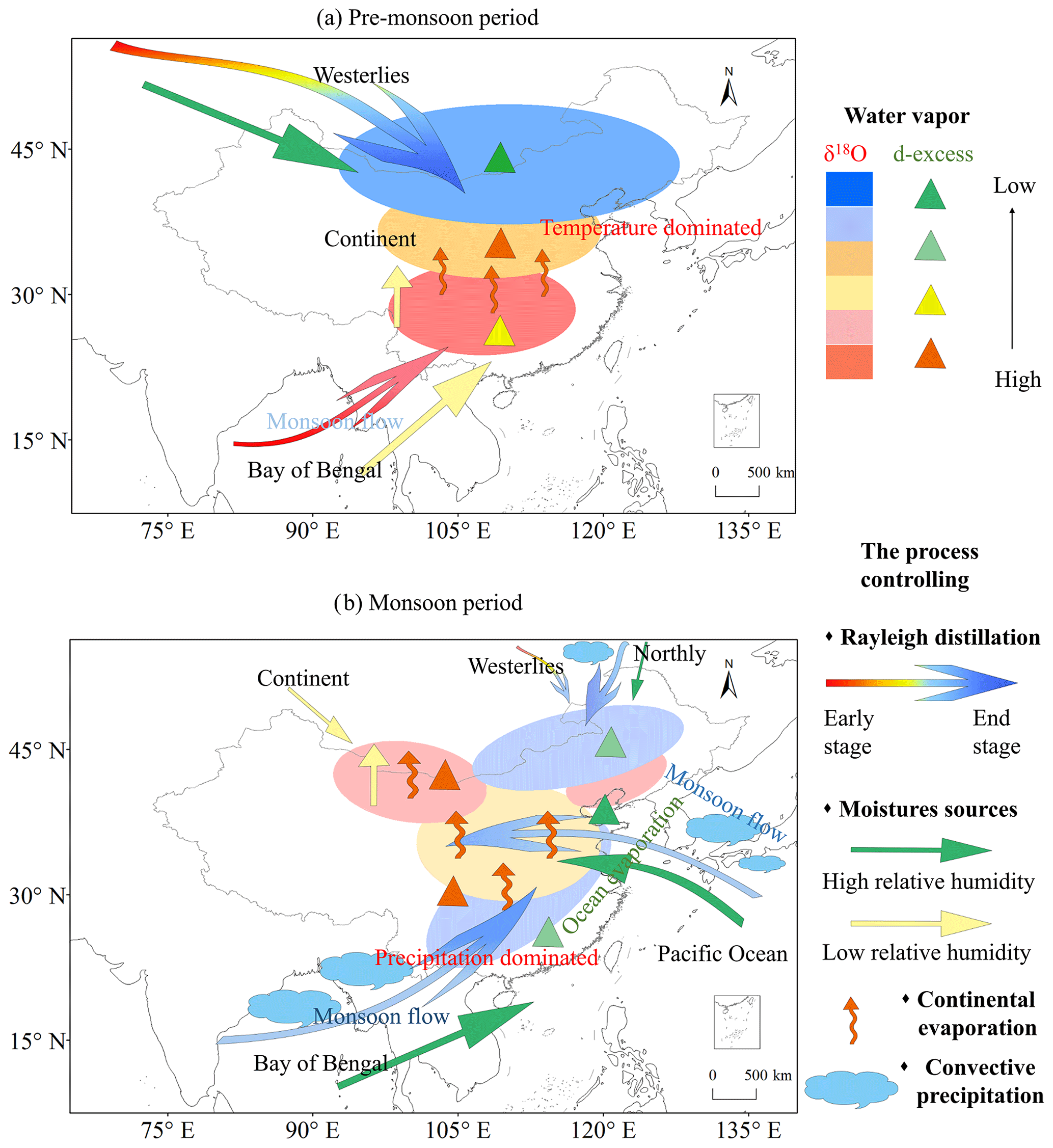
Figure 13Schematic picture summarizing the different processes controlling the observed spatial patterns and seasonality of vapor isotopes. Color gradient arrows from red to blue represent the initial to subsequent extension of the Rayleigh distillation process along the water vapor trajectory, corresponding to high to low values of δ18O. The green arrows represent high relative humidity, the yellow arrows represent low relative humidity, the orange twisted arrows represent continental recycling, blue clouds represent strong and weak convective processes, green triangle series represents low values of d-excess; and the yellow triangle series represents high values of d-excess.
Our new vehicle-based observations document spatial and seasonal variability in surface water vapor isotopic composition across a large part of China. Both during the pre-monsoon and monsoon periods, it is clear that different moisture sources and corresponding processes on transport pathways explain the spatial patterns both in vapor δ18O and d-excess (summarized in Fig. 13) as follows:
-
During the pre-monsoon period (Fig. 13a), the latitudinal gradient of vapor δ18O and d-excess were observed. The gradient in δ18O reflects the “temperature effect”, and the Rayleigh distillation appears to be the dominant control, roughly consistent with earlier studies on precipitation. Vapor in northern China, derived from westerlies, and subject to stronger Rayleigh distillation (arrows fading from red to blue), is characterized by very low isotope ratios (blue shades). Less complete Rayleigh distillation (arrows fading from red to light red) results in less depleted vapor in southern China (light red shades). The vapor d-excess in northern China is low (green triangles series), probably due to the high RH over high-latitude oceanic moisture sources for the vapor transported by the westerlies (green arrow), reducing the kinetic fractionation during ocean evaporation. In contrast, the lower RH over low-latitude moisture sources (yellow arrow) for the vapor transported to southern China leads to higher d-excess (yellow triangles series). Additional vapor sourced from continental recycling (twisted orange arrows) further increases the d-excess values in middle China. This distribution is consistent with the back-trajectory results showing that during the pre-monsoon period, the vapor in southwestern China comes from the BoB, whereas westerly moisture sources still persist in northern China.
-
During the monsoon period (Fig. 13b), the lowest vapor δ18O occurred in southwestern and northeastern China, and higher vapor δ18O values were observed in between, while the d-excess features a West–East contrast. The relatively lower vapor δ18O results from deep convection along the moisture transport pathway (blue clouds, arrows fading to blue). Meanwhile, the mixing with moisture from continental recycling (twisted orange arrows) increases the vapor δ18O values in middle and northwestern China. We observed lower vapor δ18O values when the moisture originates from the BoB than from the Pacific Ocean, consistent with stronger convection during transport. The dominance of oceanic wet moisture (green arrows) results in the lower vapor d-excess (green triangle series) in eastern China, whereas continental recycling produces higher vapor d-excess in western and northwestern China (yellow triangle series).
-
Variation in temperature drives the seasonal variations of vapor δ18O in northern China, whereas convective activity along trajectories produces low vapor δ18O during the monsoon season and drives the seasonal variation in South China. Seasonal d-excess variation reflects different conditions in the sources of vapor: in southeastern China, it is mainly due to differences in the RH over the adjacent ocean surface, while in northwestern China, it is mainly due to the vapor transported by the westerlies during the pre-monsoon period and a great contribution of continental recycling during the monsoon period.
Iso-GSM simulations and IASI satellite measurements indicate that during the pre-monsoon period, the observed temporal variations along the route across China are mainly due to multiyear seasonal mean spatial variations and marginally due to synoptic-scale variations. During the monsoon season, synoptic-scale and intraseasonal variations might contribute significantly to the apparent spatial patterns. However, since these variations have a smaller amplitude than seasonal differences, the comparison of the two snapshots do provide a representative picture of the climatological seasonal difference.
Our study on the processes governing water vapor isotopic composition at the regional scale provides an overview of the spatial distribution and seasonal variability of water isotopes and their controlling factors, providing an improved framework for interpreting the paleoclimate proxy records of the hydrological cycle in low and mid-latitudes. In particular, our results suggest a strong interaction between local factors and circulation, emphasizing the need to interpret proxy records in the context of the regional system. This also suggests the potential for changes in circulation to confound interpretations of proxy data.
The data acquired during the field campaigns can be accessed via the following: (1) https://doi.org/10.1594/PANGAEA.947606 (Wang and Tian, 2022a) and (2) https://doi.org/10.1594/PANGAEA.947627 (Wang and Tian, 2022b). Other data used can be downloaded from the corresponding websites which are listed in the text.
The supplement related to this article is available online at: https://doi.org/10.5194/acp-23-3409-2023-supplement.
LT and DW designed the research. DW, and XW conducted the field observations. JC and GJB contributed to the data calibration. ZW and KY performed the Iso-GCM simulations. DW, CR, and LT performed the analysis. All authors contributed to the discussion of the results and the final article. DW drafted the paper with contributions from all co-authors. CR, LT, GJB, LZXL, ZW and JC checked and modified the paper.
The contact author has declared that none of the authors has any competing interests.
Publisher's note: Copernicus Publications remains neutral with regard to jurisdictional claims in published maps and institutional affiliations.
The authors gratefully acknowledge NCAR/NCEP, GPCP and NOAA for provision of regional and large-scale meteorological data. We are grateful to the NOAA Air Resources Laboratory (ARL) that provided the HYSPLIT transport and dispersion model (http://ready.arl.noaa.gov/HYSPLIT.php, last access: March 2022) and the HYSPLIT-compatible meteorological dataset from GDAS. We thankfully acknowledge Yao Zhang, Xiaowen Zeng, and Min Gan for technical assistance. We thank Mingxing Tang and Ruoqun Zhang for partly participating in the field observations. We thank to Zhaowei Jing for the discussions on Rayleigh distillation lines, and we thankfully acknowledge Yao Li, Zhongyin Cai, and Rong Jiao for sharing some methods to use the Hysplit4 model. This work has been supported by the National Natural Science Foundation of China (grant nos. U2202208 and 42271143), the Applied Basic Research Foundation of Yunnan Province (grant no. 202201BF070001-021), and the Research Innovation Project for Graduate Students of Yunnan University (grant nos. 2018Z098 and 2021Y040).
This research has been supported by the National Natural Science Foundation of China (grant nos. U2202208 and 42271143), the Applied Basic Research Foundation of Yunnan Province (grant no. 202201BF070001-021), and the Research Innovation Project for Graduate Students of Yunnan University (grant nos. 2018Z098 and 2021Y040).
This paper was edited by Eliza Harris and reviewed by two anonymous referees.
Acharya, S., Yang, X., Yao, T., and Shrestha, D.: Stable isotopes of precipitation in Nepal Himalaya highlight the topographic influence on moisture transport, Quatern. Int., 565, 22–30, https://doi.org/10.1016/j.quaint.2020.09.052, 2020.
Aemisegger, F., Pfahl, S., Sodemann, H., Lehner, I., Seneviratne, S. I., and Wernli, H.: Deuterium excess as a proxy for continental moisture recycling and plant transpiration, Atmos. Chem. Phys., 14, 4029–4054, https://doi.org/10.5194/acp-14-4029-2014, 2014.
Aemisegger, F., Spiegel, J., Pfahl, S., Sodemann, H., Eugster, W., and Wernli, H.: Isotope meteorology of cold front passages: A case study combining observations and modeling, Geophys. Res. Lett., 42, 5652–5660, https://doi.org/10.1002/2015gl063988, 2015.
Aemisegger, F. and Papritz, L.: A climatology of strong large-scale ocean evaporation events. Part I: Identification, global distribution, and associated climate conditions, J. Climate, 31, 7287–7312, https://doi.org/10.1175/jcli-d-17-0591.1, 2018.
Aggarwal, P. K., Fröhlich, K., Kulkarni, K. M., and Gourcy, L. L.: Stable isotope evidence for moisture sources in the asian summer monsoon under present and past climate regimes, Geophys. Res. Lett., 31, 239–261, https://doi.org/10.1029/2004gl019911, 2004.
Araguás-Araguás, L., Froehlich, K., and Rozanski, K.: Stable isotope composition of precipitation over southeast Asia, J. Geophys. Res.-Atmos., 103, 28721–28742, https://doi.org/10.1029/98jd02582, 1998.
Bailey, A., Toohey, D., and Noone, D.: Characterizing moisture exchange between the Hawaiian convective boundary layer and free troposphere using stable isotopes in water, J. Geophys. Res.-Atmos., 118, 8208–8221, https://doi.org/10.1002/jgrd.50639, 2013.
Benetti, M., Steen-Larsen, H. C., Reverdin, G., Sveinbjörnsdóttir, Á. E., Aloisi, G., Berkelhammer, M. B., Bourlès, B., Bourras, D., De Coetlogon, G., and Cosgrove, A.: Stable isotopes in the atmospheric marine boundary layer water vapour over the Atlantic Ocean, 2012–2015, Scientific Data, 4, 160128, https://doi.org/10.1038/sdata.2016.128, 2017.
Bershaw, J., Penny, S. M., and Garzione, C. N.: Stable isotopes of modern water across the Himalaya and eastern Tibetan Plateau: Implications for estimates of paleoelevation and paleoclimate, J. Geophys. Res.-Atmos., 117, D02110, https://doi.org/10.1029/2011jd016132, 2012.
Bhattacharya, S. K., Sarkar, A., and Liang, M. C.: Vapor isotope probing of typhoons invading the Taiwan region in 2016, J. Geophys. Res.-Atmos., 127, e2022JD036578, https://doi.org/10.1029/2022jd036578, 2022.
Bonne, J.-L., Behrens, M., Meyer, H., Kipfstuhl, S., Rabe, B., Schönicke, L., Steen-Larsen, H. C., and Werner, M.: Resolving the controls of water vapour isotopes in the Atlantic sector, Nat. Commun., 10, 1632, https://doi.org/10.1038/s41467-019-09242-6, 2019.
Bony, S., Risi, C., and Vimeux, F.: Influence of convective processes on the isotopic composition (δ18O and δD) of precipitation and water vapor in the tropics: 1. Radiative-convective equilibrium and Tropical Ocean–Global Atmosphere–Coupled Ocean-Atmosphere Response Experiment (TOGA-COARE) simulations, J. Geophys. Res.-Atmos., 113, D19305, https://doi.org/10.1029/2008jd009942, 2008.
Bowen, G. J. and Revenaugh, J.: Interpolating the isotopic composition of modern meteoric precipitation, Water Resour. Res., 39, 1299, https://doi.org/10.1029/2003wr002086, 2003.
Bowen, G. J., Cai, Z., Fiorella, R. P., and Putman, A. L.: Isotopes in the Water Cycle: Regional-to Global-Scale Patterns and Applications, Annu. Rev. Earth Pl. Sc., 47, 457–479, https://doi.org/10.1146/annurev-earth-053018-060220, 2019.
Brown, J., Simmonds, I., and Noone, D.: Modeling δ18O in tropical precipitation and the surface ocean for present-day climate, J. Geophys. Res.-Atmos., 111, D05105, https://doi.org/10.1029/2004jd005611, 2006.
Brubaker, K. L., Entekhabi, D., and Eagleson, P.: Estimation of continental precipitation recycling, J. Climate, 6, 1077–1089, https://doi.org/10.1175/1520-0442(1993)006<1077:eocpr>2.0.co;2, 1993.
Cai, Z. and Tian, L.: Processes governing water vapor isotope composition in the Indo-Pacific region: Convection and water vapor transport, J. Climate, 29, 8535–8546, https://doi.org/10.1175/JCLI-D-16-0297.1, 2016.
Cai, Z., Tian, L., and Bowen, G. J.: Spatial-seasonal patterns reveal large-scale atmospheric controls on Asian Monsoon precipitation water isotope ratios, Earth Planet. Sc. Lett., 503, 158–169, https://doi.org/10.1016/j.epsl.2018.09.028, 2018.
Dansgaard, W.: Stable isotopes in precipitation, Tellus, 16, 436–468, https://doi.org/10.1111/j.2153-3490.1964.tb00181.x, 1964.
Domrös, M. and Peng, G.: The climate of China, 1st edn., Springer Science & Business Media, 56–77, ISBN 9781315202068, https://doi.org/10.4324/9781315202068-4, 2012.
Draxler, R. R. and Hess, G.: An overview of the HYSPLIT_4 modelling system for trajectories, Aust. Meteorol. Mag., 47, 295–308, 1998.
Fiorella, R. P., Bares, R., Lin, J. C., Ehleringer, J. R., and Bowen, G. J.: Detection and variability of combustion-derived vapor in an urban basin, Atmos. Chem. Phys., 18, 8529–8547, https://doi.org/10.5194/acp-18-8529-2018, 2018.
Fiorella, R. P., Bares, R., Lin, J. C., and Bowen, G. J.: Wintertime decoupling of urban valley and rural ridge hydrological processes revealed through stable water isotopes, Atmos. Environ., 213, 337–348, https://doi.org/10.1016/j.atmosenv.2019.06.022, 2019.
Galewsky, J. and Hurley, J. V.: An advection-condensation model for subtropical water vapor isotopic ratios, J. Geophys. Res.-Atmos., 115, D16116, https://doi.org/10.1029/2009jd013651, 2010.
Galewsky, J., Rella, C., Sharp, Z., Samuels, K., and Ward, D.: Surface measurements of upper tropospheric water vapor isotopic composition on the Chajnantor Plateau, Chile, Geophys. Res. Lett., 38, 198–205, https://doi.org/10.1029/2011gl048557, 2011.
Galewsky, J., Steen-Larsen, H. C., Field, R. D., Worden, J., Risi, C., and Schneider, M.: Stable isotopes in atmospheric water vapor and applications to the hydrologic cycle, Rev. Geophys., 54, 809–865, https://doi.org/10.1002/2015rg000512, 2016.
Gao, J., MassonDelmotte, V., Risi, C., He, Y., and Yao, T.: What controls precipitation δ18O in the southern Tibetan Plateau at seasonal and intra-seasonal scales? A case study at Lhasa and Nyalam, Tellus B, 65, 21043, https://doi.org/10.3402/tellusb.v65i0.21043, 2013.
Gat, J. R.: Oxygen and hydrogen isotopes in the hydrologic cycle, Annu. Rev. Earth Planet. Sc., 24, 225–262, https://doi.org/10.1146/annurev.earth.24.1.225, 1996.
Gat, J. R. and Matsui, E.: Atmospheric water balance in the Amazon Basin: an isotopic evapotranspiration model, J. Geophys. Res.-Atmos., 96, 13179–13188, https://doi.org/10.1029/91jd00054, 1991.
Gedzelman, S.: Probing hurricanes with stable isotopes of rain and water vapor, Mon. Weather Rev., 131, 1112–1127, https://doi.org/10.1175/1520-0493(2003)131<1112:phwsio>2.0.co;2, 2003.
Gorski, G., Strong, C., Good, S. P., Bares, R., Ehleringer, J. R., and Bowen, G. J.: Vapor hydrogen and oxygen isotopes reflect water of combustion in the urban atmosphere, P. Natl. Acad. Sci. USA, 112, 3247–3252, https://doi.org/10.1073/pnas.1424728112, 2015.
Gralher, B., Herbstritt, B., Weiler, M., Wassenaar, L. I., and Stumpp, C.: Correcting laser-based water stable isotope readings biased by carrier gas changes, Environ. Sci. Technol., 50, 7074–7081, https://doi.org/10.1021/acs.est.6b01124, 2016.
Guo, X., Tian, L., Wen, R., Yu, W., and Qu, D.: Controls of precipitation δ18O on the northwestern Tibetan Plateau: A case study at Ngari station, Atmos. Res., 189, 141–151, https://doi.org/10.1016/j.atmosres.2017.02.004, 2017.
He, Y., Risi, C., Gao, J., Masson-Delmotte, V., Yao, T., Lai, C. T., Ding, Y., Worden, J., Frankenberg, C., and Chepfer, H.: Impact of atmospheric convection on south Tibet summer precipitation isotopologue composition using a combination of in situ measurements, satellite data, and atmospheric general circulation modeling, J. Geophys. Res.-Atmos., 120, 3852–3871, https://doi.org/10.1002/2014jd022180, 2015.
Hou, J., Huang, Y., Oswald, W. W., Foster, D. R., and Shuman, B.: Centennial-scale compound-specific hydrogen isotope record of Pleistocene–Holocene climate transition from southern New England, Geophys. Res. Lett., 34, L19706, https://doi.org/10.1029/2007gl030303, 2007.
Johnson, J. E. and Rella, C. W.: Effects of variation in background mixing ratios of N2, O2, and Ar on the measurement of δ18O–H2O and δ2H–H2O values by cavity ring-down spectroscopy, Atmos. Meas. Tech., 10, 3073–3091, https://doi.org/10.5194/amt-10-3073-2017, 2017.
Jouzel, J., Alley, R., Cuffey, K., Dansgaard, W., Grootes, P., Hoffmann, G., Johnsen, S., Koster, R., Peel, D., and Shuman, C.: Validity of the temperature reconstruction from water isotopes in ice cores, J. Geophys. Res.-Oceans, 102, 26471–26487, https://doi.org/10.1029/97jc01283, 1997.
Khaykin, S. M., Moyer, E., Krämer, M., Clouser, B., Bucci, S., Legras, B., Lykov, A., Afchine, A., Cairo, F., Formanyuk, I., Mitev, V., Matthey, R., Rolf, C., Singer, C. E., Spelten, N., Volkov, V., Yushkov, V., and Stroh, F.: Persistence of moist plumes from overshooting convection in the Asian monsoon anticyclone, Atmos. Chem. Phys., 22, 3169–3189, https://doi.org/10.5194/acp-22-3169-2022, 2022.
Kikuchi, K.: The boreal summer intraseasonal oscillation (BSISO): A review, J. Meteorol. Soc. Jpn. Ser. II, 99, 933–972, https://doi.org/10.2151/jmsj.2021-045, 2021.
Klein, E. S., Cherry, J., Young, J., Noone, D., Leffler, A., and Welker, J.: Arctic cyclone water vapor isotopes support past sea ice retreat recorded in Greenland ice, Scientific Reports, 5, 10295, https://doi.org/10.1038/srep10295, 2015.
Kong, Y. and Pang, Z.: A positive altitude gradient of isotopes in the precipitation over the Tianshan Mountains: Effects of moisture recycling and sub-cloud evaporation, J. Hydrol., 542, 222–230, https://doi.org/10.1016/j.jhydrol.2016.09.007, 2016.
Kurita, N.: Origin of Arctic water vapor during the ice-growth season, Geophys. Res. Lett., 38, L02709, https://doi.org/10.1029/2010gl046064, 2011.
Li, Y., An, W., Pang, H., Wu, S. Y., Tang, Y., Zhang, W., and Hou, S.: Variations of Stable Isotopic Composition in Atmospheric Water Vapor and their Controlling Factors – A 6-Year Continuous Sampling Study in Nanjing, Eastern China, J. Geophys. Res.-Atmos., 125, e2019JD031697, https://doi.org/10.1029/2019jd031697, 2020.
Li, Y., Aemisegger, F., Riedl, A., Buchmann, N., and Eugster, W.: The role of dew and radiation fog inputs in the local water cycling of a temperate grassland during dry spells in central Europe, Hydrol. Earth Syst. Sci., 25, 2617–2648, https://doi.org/10.5194/hess-25-2617-2021, 2021.
Liebmann, B. and Smith, C. A.: Description of a complete (interpolated) outgoing longwave radiation dataset, B. Am. Meteorol. Soc., 77, 1275–1277, 1996.
Liu, J., Xiao, C., Ding, M., and Ren, J.: Variations in stable hydrogen and oxygen isotopes in atmospheric water vapor in the marine boundary layer across a wide latitude range, J. Environ. Sci., 26, 2266–2276, https://doi.org/10.1016/j.jes.2014.09.007, 2014.
Liu, Y., Cobb, K. M., Song, H., Li, Q., Li, C.-Y., Nakatsuka, T., An, Z., Zhou, W., Cai, Q., and Li, J.: Recent enhancement of central Pacific El Niño variability relative to last eight centuries, Nat. Commun., 8, 15386, https://doi.org/10.1038/ncomms15386, 2017.
McKinney, C. R., McCrea, J. M., Epstein, S., Allen, H., and Urey, H. C.: Improvements in mass spectrometers for the measurement of small differences in isotope abundance ratios, Rev. Sci. Instrum., 21, 724–730, https://doi.org/10.1063/1.1745698, 1950.
Mei'e, R., Renzhang, Y., and Haosheng, B.: An outline of China's physical geography, The World in Outline, 497–520, https://doi.org/10.1017/cbo9781316530399.026, 1985.
Merlivat, L. and Jouzel, J.: Global climatic interpretation of the deuterium-oxygen 18 relationship for precipitation, J. Geophys. Res.-Oceans, 84, 5029–5033, https://doi.org/10.1029/jc084ic08p05029, 1979.
Noone, D.: The influence of midlatitude and tropical overturning circulation on the isotopic composition of atmospheric water vapor and Antarctic precipitation, J. Geophys. Res.-Atmos., 113, D04102, https://doi.org/10.1029/2007jd008892, 2008.
Noone, D.: Pairing Measurements of the Water Vapor Isotope Ratio with Humidity to Deduce Atmospheric Moistening and Dehydration in the Tropical Midtroposphere, J. Climate, 25, 4476–4494, https://doi.org/10.1175/jcli-d-11-00582.1, 2012.
Pausata, F. S. R., Battisti, D. S., Nisancioglu, K. H., and Bitz, C. M.: Chinese stalagmite δ18O controlled by changes in the Indian monsoon during a simulated Heinrich event, Nat. Geosci., 4, 474–480, https://doi.org/10.1038/ngeo1169, 2011.
Pfahl, S. and Sodemann, H.: What controls deuterium excess in global precipitation?, Clim. Past, 10, 771–781, https://doi.org/10.5194/cp-10-771-2014, 2014.
Putman, A. L., Fiorella, R. P., Bowen, G. J., and Cai, Z.: A global perspective on local meteoric water lines: Meta-analytic insight into fundamental controls and practical constraints, Water Resour. Res., 55, 6896–6910, https://doi.org/10.1029/2019wr025181, 2019.
Risi, C., Bony, S., and Vimeux, F.: Influence of convective processes on the isotopic composition (δ18O and δD) of precipitation and water vapor in the tropics: 2. Physical interpretation of the amount effect, J. Geophys. Res.-Atmos., 113, D19306, https://doi.org/10.1029/2008jd009943, 2008a.
Risi, C., Bony, S., Vimeux, F., Descroix, L., Ibrahim, B., Lebreton, E., Mamadou, I., and Sultan, B.: What controls the isotopic composition of the African monsoon precipitation? Insights from event-based precipitation collected during the 2006 AMMA field campaign, Geophys. Res. Lett., 35, 851–854, https://doi.org/10.1029/2008gl035920, 2008b.
Risi, C., Bony, S., Vimeux, F., and Jouzel, J.: Water-stable isotopes in the LMDZ4 general circulation model: Model evaluation for present-day and past climates and applications to climatic interpretations of tropical isotopic records, J. Geophys. Res.-Atmos., 115, D12118, https://doi.org/10.1029/2009jd013255, 2010.
Risi, C., Noone, D., Worden, J., Frankenberg, C., Stiller, G., Kiefer, M., Funke, B., Walker, K., Bernath, P., Schneider, M., Wunch, D., Sherlock, V., Deutscher, N., Griffith, D., Wennberg, P. O., Strong, K., Smale, D., Mahieu, E., Barthlott, S., Hase, F., Garcia, O., Notholt, J., Warneke, T., Toon, G., Sayres, D., Bony, S., Lee, J., Brown, D., Uemura, R., and Sturm, C.: Process-evaluation of tropospheric humidity simulated by general circulation models using water vapor isotopologues: 1. Comparison between models and observations, J. Geophys. Res.-Atmos., 117, D05303, https://doi.org/10.1029/2011jd016621, 2012.
Risi, C., Landais, A., Winkler, R., and Vimeux, F.: Can we determine what controls the spatio-temporal distribution of d-excess and 17O-excess in precipitation using the LMDZ general circulation model?, Clim. Past, 9, 2173–2193, https://doi.org/10.5194/cp-9-2173-2013, 2013a.
Risi, C., Noone, D., Frankenberg, C., and Worden, J.: Role of continental recycling in intraseasonal variations of continental moisture as deduced from model simulations and water vapor isotopic measurements, Water Resour. Res., 49, 4136–4156, https://doi.org/10.1002/wrcr.20312, 2013b.
Roca, R., Chambon, P., Jobard, I., Kirstetter, P.-E., Gosset, M., and Bergès, J. C.: Comparing satellite and surface rainfall products over West Africa at meteorologically relevant scales during the AMMA campaign using error estimates, J. Appl. Meteorol. Clim., 49, 715–731, https://doi.org/10.1175/2009jamc2318.1, 2010.
Salati, E., Dall'Olio, A., Matsui, E., and Gat, J. R.: Recycling of water in the Amazon basin: an isotopic study, Water Resour. Res., 15, 1250–1258, https://doi.org/10.1029/wr015i005p01250, 1979.
Salmon, O. E., Welp, L. R., Baldwin, M. E., Hajny, K. D., Stirm, B. H., and Shepson, P. B.: Vertical profile observations of water vapor deuterium excess in the lower troposphere, Atmos. Chem. Phys., 19, 11525–11543, https://doi.org/10.5194/acp-19-11525-2019, 2019.
Samuels-Crow, K. E., Galewsky, J., Sharp, Z. D., and Dennis, K. J.: Deuterium excess in subtropical free troposphere water vapor: Continuous measurements from the Chajnantor Plateau, northern Chile, Geophys. Res. Lett., 41, 8652–8659, https://doi.org/10.1002/2014gl062302, 2015.
Sánchez-Murillo, R., Durán-Quesada, A. M., Esquivel-Hernández, G., Rojas-Cantillano, D., Birkel, C., Welsh, K., Sánchez-Llull, M., Alonso-Hernández, C. M., Tetzlaff, D., and Soulsby, C.: Deciphering key processes controlling rainfall isotopic variability during extreme tropical cyclones, Nat. Commun., 10, 4321, https://doi.org/10.1038/s41467-019-12062-3, 2019.
Saranya, P., Krishan, G., Rao, M., Kumar, S., and Kumar, B.: Controls on water vapor isotopes over Roorkee, India: Impact of convective activities and depression systems, J. Hydrol., 557, 679–687, https://doi.org/10.1016/j.jhydrol.2017.12.061, 2018.
Schmidt, M., Maseyk, K., Lett, C., Biron, P., Richard, P., Bariac, T., and Seibt, U.: Concentration effects on laser-based δ18O and δ2H measurements and implications for the calibration of vapour measurements with liquid standards, Rapid Commun. Mass Sp., 24, 3553–3561, https://doi.org/10.1002/rcm.4813, 2010.
Schneider, D. P. and Noone, D. C.: Spatial covariance of water isotope records in a global network of ice cores spanning twentieth-century climate change, J. Geophys. Res.-Atmos., 112, D18105, https://doi.org/10.1029/2007jd008652, 2007.
Shi, X., Risi, C., Pu, T., Lacour, J. l., Kong, Y., Wang, K., He, Y., and Xia, D.: Variability of isotope composition of precipitation in the southeastern Tibetan Plateau from the synoptic to seasonal time scale, J. Geophys. Res.-Atmos., 125, e2019JD031751, https://doi.org/10.1029/2019jd031751, 2020.
Steen-Larsen, H. C., Johnsen, S. J., Masson-Delmotte, V., Stenni, B., Risi, C., Sodemann, H., Balslev-Clausen, D., Blunier, T., Dahl-Jensen, D., Ellehøj, M. D., Falourd, S., Grindsted, A., Gkinis, V., Jouzel, J., Popp, T., Sheldon, S., Simonsen, S. B., Sjolte, J., Steffensen, J. P., Sperlich, P., Sveinbjörnsdóttir, A. E., Vinther, B. M., and White, J. W. C.: Continuous monitoring of summer surface water vapor isotopic composition above the Greenland Ice Sheet, Atmos. Chem. Phys., 13, 4815–4828, https://doi.org/10.5194/acp-13-4815-2013, 2013.
Steen-Larsen, H. C., Risi, C., Werner, M., Yoshimura, K., and Masson-Delmotte, V.: Evaluating the skills of isotope-enabled General Circulation Models against in-situ atmospheric water vapor isotope observations, J. Geophys. Res., 122, 246–263, https://doi.org/10.1002/2016jd025443, 2017.
Tan, M.: Circulation effect: response of precipitation delta δ18O to the ENSO cycle in monsoon regions of China, Clim. Dynam., 42, 1067–1077, https://doi.org/10.1007/s00382-013-1732-x, 2014.
Terzer-Wassmuth, S., Wassenaar, L. I., Welker, J. M., and Araguás-Araguás, L. J.: Improved high-resolution global and regionalized isoscapes of δ18O, δ2H and d-excess in precipitation, Hydrol. Process., 35, e14254, https://doi.org/10.1002/hyp.14254, 2021.
Thompson, L. G.: Ice core evidence for climate change in the Tropics: implications for our future, Quaternary Sci. Rev., 19, 19–35, https://doi.org/10.1016/s0277-3791(99)00052-9, 2000.
Thompson, L. G., Yao, T., Mosley-Thompson, E., Davis, M., Henderson, K., and Lin, P.-N.: A high-resolution millennial record of the South Asian monsoon from Himalayan ice cores, Science, 289, 1916–1919, https://doi.org/10.1126/science.289.5486.1916, 2000.
Thompson, L. O., Mosley-Thompson, E., Davis, M., Lin, P., Yao, T., Dyurgerov, M., and Dai, J.: “Recent warming”: ice core evidence from tropical ice cores with emphasis on Central Asia, Global Planet. Change, 7, 145–156, https://doi.org/10.1016/0921-8181(93)90046-q, 1993.
Thompson, L. O., Yao, T., Davis, M., Henderson, K., Mosley-Thompson, E., Lin, P.-N., Beer, J., Synal, H.-A., Cole-Dai, J., and Bolzan, J.: Tropical climate instability: The last glacial cycle from a Qinghai-Tibetan ice core, Science, 276, 1821–1825, https://doi.org/10.1126/science.276.5320.1821, 1997.
Thurnherr, I., Kozachek, A., Graf, P., Weng, Y., Bolshiyanov, D., Landwehr, S., Pfahl, S., Schmale, J., Sodemann, H., Steen-Larsen, H. C., Toffoli, A., Wernli, H., and Aemisegger, F.: Meridional and vertical variations of the water vapour isotopic composition in the marine boundary layer over the Atlantic and Southern Ocean, Atmos. Chem. Phys., 20, 5811–5835, https://doi.org/10.5194/acp-20-5811-2020, 2020.
Tian, L., Yao, T., Schuster, P. F., White, J. W. C., Ichiyanagi, K., Pendall, E., Pu, J., and Yu, W.: Oxygen-18 concentrations in recent precipitation and ice cores on the Tibetan Plateau, J. Geophys. Res.-Atmos., 108, 4293, https://doi.org/10.1029/2002jd002173, 2003.
Tian, L., Yao, T., Li, Z., MacClune, K., Wu, G., Xu, B., Li, Y., Lu, A., and Shen, Y.: Recent rapid warming trend revealed from the isotopic record in Muztagata ice core, eastern Pamirs, J. Geophys. Res.-Atmos., 111, D13103, https://doi.org/10.1029/2005jd006249, 2006.
Tian, L., Yao, T., MacClune, K., White, J. W. C., Schilla, A., Vaughn, B., Vachon, R., and Ichiyanagi, K.: Stable isotopic variations in west China: A consideration of moisture sources, J. Geophys. Res.-Atmos., 112, D10112, https://doi.org/10.1029/2006jd007718, 2007.
Tian, L., Yu, W., Schuster, P. F., Wen, R., Cai, Z., Wang, D., Shao, L., Cui, J., and Guo, X.: Control of seasonal water vapor isotope variations at Lhasa, southern Tibetan Plateau, J. Hydrol., 580, 124237, https://doi.org/10.1016/j.jhydrol.2019.124237, 2020.
Van Breukelen, M., Vonhof, H., Hellstrom, J., Wester, W., and Kroon, D.: Fossil dripwater in stalagmites reveals Holocene temperature and rainfall variation in Amazonia, Earth Planet. Sc. Lett., 275, 54–60, https://doi.org/10.1016/j.epsl.2008.07.060, 2008.
Vimeux, F., Gallaire, R., Bony, S., Hoffmann, G., and Chiang, J. C.: What are the climate controls on δD in precipitation in the Zongo Valley (Bolivia)? Implications for the Illimani ice core interpretation, Earth Planet. Sc. Lett., 240, 205–220, https://doi.org/10.1016/j.epsl.2005.09.031, 2005.
Wallace, J. M. and Hobbs, P. V.: Atmospheric science: an introductory survey, International Geophysics Series, ISSN 0074-6142, Elsevier Academic Press, 483 pp., ISBN 012732951X, 9780127329512 2006.
Wang, B.: Rainy season of the Asian–Pacific summer monsoon, J. Climate, 15, 386–398, https://doi.org/10.1175/1520-0442(2002)015<0386:rsotap>2.0.co;2, 2002.
Wang, B. and Xu, X.: Northern Hemisphere summer monsoon singularities and climatological intraseasonal oscillation, J. Climate, 10, 1071–1085, https://doi.org/10.1175/1520-0442(1997)010<1071:nhsmsa>2.0.co;2, 1997.
Wang, D. and Tian, L.: Vehicle-based in-situ observations of the water vapor isotopic composition across China during the monsoon season 2018, PANGAEA [data set], https://doi.org/10.1594/PANGAEA.947606, 2022a.
Wang, D. and Tian, L.: Vehicle-based in-situ observations of the water vapor isotopic composition across China during the pre-monsoon season 2019, PANGAEA [data set], https://doi.org/10.1594/PANGAEA.947627, 2022b.
Wang, D. and Wang, K.: Isotopes in precipitation in China (1986–1999), Sci. China Ser. E, 44, 48–51, https://doi.org/10.1007/bf02916789, 2001.
Wang, G., Lan, H., and Liu, Z.: Stable isotope record of super typhoon Lekima (2019), Atmos. Res., 264, 105822, https://doi.org/10.1016/j.atmosres.2021.105822, 2021.
Wang, Q. and Zhang, L.: Analysis of the August 2018 atmosphere circulation and weather, Meteorological Monthly, 44, 1501–1508, 2018.
West, J. B., Bowen, G. J., Dawson, T. E., and Tu, K. P.: Isoscapes: understanding movement, pattern, and process on Earth through isotope mapping, Springer Nature, 511 pp., ISBN 9789048133536, 2009.
Winnick, M. J., Chamberlain, C. P., Caves, J. K., and Welker, J. M.: Quantifying the isotopic “continental effect”, Earth Planet. Sc. Lett., 406, 123–133, https://doi.org/10.1016/j.epsl.2014.09.005, 2014.
Worden, J., Noone, D., Bowman, K., and Tropospheric Emission, S.: Importance of rain evaporation and continental convection in the tropical water cycle, Nature, 445, 528–532, https://doi.org/10.1038/nature05508, 2007.
Wright, H. E.: Global climates since the last glacial maximum, University of Minnesota Press Minneapolis, 569 pp., ISBN 97808166214530816621454, 1993.
Yao, T., Ding, L., Pu, J., Liu, J., and Yang, Z.: Characteristic of δ18O in snow and its relation with moisture sources in Tanggula Mountains, Tibetan Plateau, Chinese Sci. Bull., 36, 1570–1573, 1991.
Yoshimura, K. and Kanamitsu, M.: Specification of External Forcing for Regional Model Integrations, Mon. Weather Rev., 137, 1409–1421, https://doi.org/10.1175/2008mwr2654.1, 2009.
- Abstract
- Introduction
- Data and methods
- Spatial and seasonal variations
- Understanding the factors controlling the spatial and seasonal distributions
- Conclusion
- Data availability
- Author contributions
- Competing interests
- Disclaimer
- Acknowledgements
- Financial support
- Review statement
- References
- Supplement