the Creative Commons Attribution 4.0 License.
the Creative Commons Attribution 4.0 License.
 | 13 Mar 2023
Profile-based estimated inversion strength
Zhenquan Wang
Jian Yuan
Yifan Chen
Tiancheng Tong
To better measure the planetary boundary layer inversion strength (IS), a novel profile-based method of estimated inversion strength (EISp) is developed using the ERA5 daily reanalysis data. The EISp is designed to estimate the IS based on the thinnest possible reanalysis layer above the lifting condensation level encompassing the inversion layer. At a ground-based site in North America, the EISp correlates better with the radiosonde-detected IS (R=0.74) than the lower-tropospheric stability (LTS, R=0.53) and the estimated inversion strength (EIS, R=0.45). The daily variance in low cloud cover (LCC) explained by the EISp is twice that explained by the LTS and EIS. Higher correlations between the EISp and the radiosonde-detected IS are also found at other radiosonde stations of the subtropics and midlatitudes.
Analysis of LCC observed by geostationary satellites and the Moderate Resolution Imaging Spectroradiometer shows that the EISp explains 78 % of the annual mean LCC spatial variance over global oceans and land, which is larger than that explained by the LTS and EIS (48 % and 13 %). Over tropical and subtropical low-cloud-prevailing eastern oceans, the LCC range is more resolved by the EISp (48 %) than by the LTS and EIS (37 % and 36 %). Furthermore, the EISp explains a larger fraction (32 %) in the daily LCC variance as compared to that explained by the LTS and EIS (14 % and 16 %). The seasonal LCC variance explained by the EISp is 89 %, which is larger than that explained by the LTS and EIS (80 % and 70 %). The LCC–EISp relationship is more uniform across various timescales than the LCC–LTS and LCC–EIS relationships. It is suggested that the EISp is a better cloud-controlling factor for LCC and is likely a useful external environmental constraint for process-level studies in which there is a need to control for large-scale meteorology in order to isolate the cloud responses to aerosols on short timescales.
- Article
(6856 KB) - Full-text XML
- BibTeX
- EndNote


The inversion strength (IS) of the planetary boundary layer (PBL) is an important factor that affects PBL moisture trapping and low-cloud formation. Strong IS inhibits the dry air above the inversion from being incorporated into the PBL and traps moisture below the inversion to favor greater cloud cover (Wood and Bretherton, 2006; Mauger and Norris, 2010). In contrast, weak IS promotes the drying effect of entrained air from the free troposphere and reduces the PBL moisture to decrease cloud cover (Bretherton and Wyant, 1997; Myers and Norris, 2013). Currently, two approximate measures of the IS based on reanalysis data are widely used as meteorological constraints on low cloud cover (LCC): the lower-tropospheric stability (LTS; Klein and Hartmann, 1993) and the estimated inversion strength (EIS; Wood and Bretherton, 2006). They are both defined as a two-level potential temperature (θ) difference between the 700 hPa level and the surface, but for the EIS the moist adiabatic θ increase above the lifting condensation level (LCL) is additionally removed. The EIS can be combined with the moisture difference between the 700 hPa and surface to form a new stability index, the estimated cloud-top entrainment index (ECTEI). The ECTEI and the EIS have similar correlations with LCC on the seasonal timescales (Kawai et al., 2017).
The LTS and EIS are the best known and most widely used cloud-controlling factors for the explanation of LCC variations. Enhanced LTS can moisten PBLs and has been shown to precede LCC changes by about 24–36 h (Mauger and Norris, 2010; Klein, 1997). Similarly, Myers and Norris (2013) found that the EIS is the main cause of LCC variations, and enhanced subsidence actually decreases LCC for the same value of the EIS. These LCC–LTS and LCC–EIS relationships are vital for not only separating observational aerosol effects on clouds from meteorological influences (L'ecuyer et al., 2009; Rosenfeld et al., 2019; Murray-Watson and Gryspeerdt, 2022; Coopman et al., 2016) but also estimating low cloud climate feedbacks (Klein et al., 2017; Sherwood et al., 2020). In terms of aerosol–cloud interactions, the LTS and EIS can be used to constrain meteorological influences and thus largely reduce the confounding influence of meteorology to separate aerosol effects on low clouds (Mauger and Norris, 2007; Coopman et al., 2016), since LCC variations are most explained by the LTS and EIS among all the LCC-controlling meteorological factors (Stevens and Brenguier, 2009). Without strong cloud-controlling factors, the confounding influence of meteorology is poorly constrained, and over half of the relationship between aerosol optical depth and LCC results from meteorological covariations (Gryspeerdt et al., 2016). Besides, in climate projections, Webb et al. (2012) found that most climate models cannot reproduce the observational LCC–LTS and LCC–EIS relationship, and thus low cloud feedbacks have the largest spread among climate models. To help constrain future climate projections, the LTS- and EIS-induced low cloud feedback can be more accurately estimated by multiplying the observational LCC–LTS and LCC–EIS sensitivity by the LTS and EIS changes of climate model projections (Webb et al., 2012; Qu et al., 2014; Myers and Norris, 2016; Klein et al., 2017; Mccoy et al., 2017; Myers et al., 2021; Seethala et al., 2015; Kawai et al., 2017).
Although the LTS and EIS are best correlated with LCC among all meteorological factors, the LTS and EIS only explain a small portion of LCC variance on short timescales. A total of 12 % of daily LCC variance are explained by the LTS, but when the monthly means are subtracted from the data, only 4.8 % of the daily LCC variance are explained by the LTS at the subtropical ocean weather station (OWS) N (Klein, 1997). Similarly, when the monthly means are removed, only 4 % of daily LCC variance are explained by the EIS over the typical subtropical eastern oceans (Szoeke et al., 2016). LCC on daily time scales is not as well explained by the LTS/EIS as the LCC on longer time scales. But the LCC sensitivity to LTS/EIS is assumed to be time-scale invariant to estimate the LTS/EIS-induced low cloud feedback and thus leads to some uncertainty (Klein et al., 2017). The explanation for the variant relationship between LCC and LTS/EIS across different time scales is not clear. And it is also not known whether the LTS and EIS can approximate the IS with the same accuracy across different time scales.
Grounded on the well-mixed condition, the PBL's thermal structure is relatively simple, and both the LTS and EIS are likely to be good measures of IS. However, the actual PBL thermal stratification may not always be well mixed. In deep decoupled PBLs, a strong stratification with a large θ increase between cloud layers and surface-mixed layers would exist (Jones et al., 2011; Nicholls, 1984). In this case, both the LTS and EIS likely count the stable layer of the decoupling into the IS estimates and thus overestimate the real IS atop the PBL. Previous studies also showed that the free-tropospheric lapse rate has small biases and large spreads, although on average it is close to the moist adiabat on daily timescales (Wood and Bretherton, 2006). Thus, further refinements of the algorithm for IS estimations are possible if we can reduce the biases and errors resulting from the deviations from the well-mixed conditions. Given the importance of the LTS and EIS for studies of cloud–aerosol interactions and climate predictions, a better measure of the IS can lead to more accurate quantification and increasing confidence in these fields. Based on the previous EIS framework, this study further establishes a profile-based EIS (EISp) algorithm to take advantages of the reanalysis and thus to estimate more accurately the IS.
This paper is laid out as follows: Sect. 2 briefly describes the observation and reanalysis data and introduces methodologies used in our analysis; Sect. 3 illustrates the development and validation of the new EISp; Sect. 4 evaluates the relationship between LCC and EISp at the global scale, with conclusions in Sect. 5.
Data used in this study include the following: (1) high-vertical-resolution radiosondes and cloud radar and lidar observations from the ground site of the Atmospheric Radiation Measurement (ARM) Program; (2) radiosondes of several subtropical and midlatitude stations from the Integrated Global Radiosonde Archive (IGRA) of the National Oceanic and Atmospheric Administration (NOAA); (3) global satellite observations of LCC; (4) the fifth-generation atmospheric reanalysis from the European Centre for Medium-Range Weather Forecasts (ECMWF). Methodologies of data processing are also introduced.
2.1 Radiosonde and cloud observations at the ground-based sites
Long-term ground-based observations are from two sites of the ARM Program at the southern Great Plains (SGP) and the eastern North Atlantic (ENA) (Ackerman and Stokes, 2003). ARM was established by the US Department of Energy's Office of Biological and Environmental Research to provide an observational basis for studying the Earth's climate. At the SGP observatory (97.5∘ W, 36.6∘ N and 318 m above sea level) and the ENA observatory (28.1∘ W, 39.5∘ N and 30 m a.s.l.), high-quality radiosondes and cloud radar and lidar observations are provided to validate the new algorithm of EISp and to investigate the relationship of IS and IS estimates (i.e., LTS, EIS and EISp) with LCC. However, the ENA is located on Graciosa Island in the midlatitude ocean, where low clouds frequently occur but with no inversion (Norris, 1998) so that it is not an ideal site to investigate the relationship of LCC with IS. Thus, the observations at the ENA are only used to validate the accuracy of EISp by comparing with the radiosonde-measured IS.
The atmospheric temperature, relative humidity (RH) and pressure profiles measured by the SGP balloon-borne sounding system (SONDE) from 2002 to 2011 are used. The sondes at the SGP are launched four times a day at 05:30, 11:30, 17:30 and 23:30 UTC. To avoid the diurnal-cycle influence on our analysis, only the sondes launched at 17:30 UTC (11:00 LT) are used. At this time, the PBL is relatively more well mixed by turbulence with more uniform vertical distribution of θ than at the other times of the day (Liu and Liang, 2010). The data at different times are also tested, and they come to similar results. The precision of the sonde-measured temperature, RH and pressure is 0.1 K, 1 % and 0.1 hPa (Ken, 2001), respectively. Their accuracy is 0.2 K, 2 % and 0.5 hPa, respectively (Ken, 2001). Its vertical resolution is normally about 10 m from the ground level up to 30 km. The sonde temporal resolution is less than 2.5 s with 6m s−1 ascent rate at the 1000 hPa level. The θ profile is computed from the sonde temperature and pressure profiles as follows:
where Ra is the specific gas constant of dry air, and cpa is the specific heat capacity for dry air at constant pressures. T and p are the sonde temperature and pressure. The θ vertical-gradient ( profile is derived from the θ difference between two adjacent levels:
where z is the height above the ground level (AGL). The subscript “i” indicates the ith level detected by the sonde.
Cloud profiles are observed every 10 s by the 35 GHz millimeter-wavelength cloud radar and the micro-pulse lidar from 2002 to 2011 at the SGP. The ARM best-estimate cloud radiation measurement (ARMBECLDRAD) product is used (Chen and Xie, 1996), which provides radar and lidar cloud profiles derived from the Active Remote Sensing of Clouds (ARSCL). Its vertical resolution is 45 m. To match the sonde launched at 17:30 UTC, the hourly segment of cloud measurements during 17:00–18:00 UTC is used. The cloud base and top heights of an hourly segment are recognized as the lowest and highest levels of cloud layers (non-zero cloud fraction) detected in that hourly segment. In a cloud profile, distinct cloud layers are separated by a minimum distance threshold of 250 m (Li et al., 2011). Low clouds are defined as having a cloud base height of less than 3 km and a top height of less than 4 km. These low clouds are dominated by stratus, stratocumulus and shallow cumulus clouds (Dong et al., 2005). Segments of solely other types of clouds but no low cloud are excluded in our analysis. Segments that have low clouds but with other clouds aloft are kept. The LCC of an hourly segment is defined as the ratio of the number of cloudy profiles to the total number of profiles in that segment.
These hourly segments are further sorted into three categories: clear sky, coupled cloudy and decoupled cloudy segments. Clear sky segments are those in which no cloud is present within that segment. The coupled and decoupled cloudy segments are segments containing low clouds in coupled and decoupled PBLs, respectively. A straightforward indicator to distinguish coupled and decoupled PBLs is the height difference between the cloud base and the LCL (Δzb) (Jones et al., 2011). When the PBL is well mixed, Δzb is close to zero, but in the decoupled PBLs the cloud and subcloud layers would be separated by a stable layer, and the LCL may diverge from the cloud base by hundreds of meters with large Δzb (Nicholls, 1984; Jones et al., 2011). The threshold value of Δzb is empirical; for different instrument capability, vertical resolution and locations, the threshold may be a little different. In reference to the linear least-squares fit between Δzb and Δθ in Jones et al. (2011), where 150 m of Δzb correspond to 0.5 K of the θ difference in the subcloud layer, a similar linear relationship is found, but the slope is a little different in that 180 m of Δzb corresponds to 0.5 K of the θ difference at the SGP site. Thus, at the SGP site, a threshold value of 180 m for Δzb is used to distinguish coupled and decoupled PBLs.
At the ENA, data of radiosondes and LCC from 2014 to 2020 are used. The data product and processing method of the ENA site are the same as those of the SGP. The ENA site is characterized by marine stratocumulus clouds but at midlatitudes, where the correlation between LCC and IS is much weaker as compared to that at the SGP. This will be verified and discussed later.
2.2 Radiosonde stations of subtropics and midlatitudes
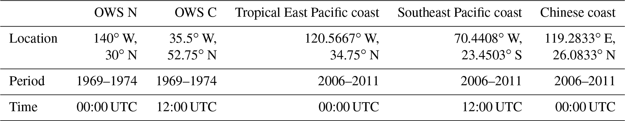
The IGRA of NOAA collects radiosondes from globally distributed stations (Durre et al., 2018; Durre et al., 2006). The radiosonde temperature, RH, pressure and geopotential height profiles in the IGRA are used. The θ and θ gradient profiles are computed from Eqs. (1) and (2). These atmospheric parameters of radiosondes are available at the standard pressure levels (1000, 925, 850, 700 and 500 hPa) or variable levels. It provides reliable instantaneous observations for the PBL IS (see definitions in Sect. 2.5). However, most low-cloud-dominated regions are over the ocean with no available radiosondes in the IGRA. Thus, five radiosonde stations with relatively higher occurrence frequencies of low clouds are selected: the OWS N in the subsidence and steady trade wind circulation of the northeast Pacific (Klein, 1997; Klein et al., 1995), the OWS C in the frequently decoupled PBLs of the North Atlantic (Norris, 1998), the tropical East Pacific coast with the classic stratocumulus condition (Albrecht et al., 1995), the southeast Pacific coast with the stratocumulus-capped PBLs (Bretherton et al., 2004) and the southeast Chinese coast of subtropical low-cloud domains (Klein and Hartmann, 1993). Locations, observational period and time of data for each station are listed in Table 1.
Table 1The location, observational period and time of the IGRA radiosonde stations.
2.3 Global LCC observations
Global LCC observations of the geostationary satellites (GEOs) and the Moderate Resolution Imaging Spectroradiometer (MODIS) on board the Aqua and Terra satellites are provided by the Clouds and the Earth's Radiant Energy System (CERES) project (Doelling et al., 2013, 2016; Trepte et al., 2019). Global hourly LCC between 60∘ S and 60∘ N during 2006–2011 is used. It is available in the Synoptic 1 ∘ (SYN1deg) edition 4.1 product of the CERES project (Doelling et al., 2013, 2016; Trepte et al., 2019). The GEO-MODIS LCC here refers to the cloud area fraction of the identified cloudy pixels with cloud top pressure above 700 hPa divided by the total number of pixels in the 1 grids. The MODIS pixel-level cloud identification is based on the CERES MODIS cloud algorithm (Minnis et al., 2008, 2011). The sampling frequency of clouds derived from the MODIS narrowband radiance is four times a day (two from each of the Aqua Terra). GEOs with radiances calibrated against the MODIS provide hourly cloud retrievals between MODIS observations (Doelling et al., 2013). The GEO cloudy pixel identification is also based on the CERES-MODIS-like cloud algorithm to achieve more uniform MODIS and GEO clouds. An advantage of this product over cloud retrievals of the first-generation GEO is that the CERES project uses the latest generation of the GEO imager capability with more additional channels to enhance the accuracy of cloud retrievals (Doelling et al., 2016). Hourly LCC is used to match the IGRA radiosondes. Daily LCC used in Sect. 4 is the mean of the full-day hourly GEO-MODIS LCC from the CERES SYN1deg edition 4.1 product (Doelling et al., 2016).
2.4 The fifth-generation ECMWF atmospheric reanalysis (ERA5)
Reanalysis data from the ECMWF are to provide the atmospheric profile information. The ERA5 combines observations with model outputs by the 4D-Var assimilation to achieve the 1 h resolution (Hersbach et al., 2020). The hourly atmospheric temperature, RH, geopotential profiles in the ERA5 dataset are used to match the SGP, IGRA and GEO-MODIS observations. The θ and θ gradient profiles are computed based on Eqs. (1) and (2). Atmospheric profiles at the 16 pressure levels between 500 and 1000 hPa are available. At the SGP site, the ERA5 atmospheric profiles between the years 2002 and 2011 at the grid point (97.5∘ W, 36.625∘ N) nearest to the SGP site (within about 2.8 km) are used. For the IGRA radiosonde stations, the ERA5 hourly data of the 0.125∘ grid point nearest to them during the same observational period are used. At the global scale, the ERA5 atmospheric profiles are averaged to 1∘ resolution data, centered at 0.5∘, 1.5 during the years between 2006 and 2011. This resolution is consistent with the global LCC data. Those three metrics, LTS, EIS and EISp, are then computed based on the 3 h 1∘ ERA5 atmospheric profiles. All metrics at longer (i.e., from daily to seasonal) timescales are computed from the 3 h metrics.
2.5 LTS, EIS and radiosonde-measured IS
The LTS and EIS over the ocean are defined as follows:
where θ and z are, respectively, the potential temperature and the height. The subscripts “700 hPa”, “0” and “LCL” indicate the levels of 700 hPa, 1000 hPa and the LCL, respectively. zLCL is calculated using temperature and RH at 1000 hPa based on the exact expression in Romps (2017), indicating the height at which an air parcel would saturate if lifted adiabatically. Γm is the moist adiabatic θ gradient at 850 hPa calculated using the mean temperature of the 1000 and 700 hPa levels. Γm can be calculated as follows:
qs is the saturated mass fraction of water vapor. Lv is the latent heat of vaporization. Rv is the specific gas constant for water vapor.
Over land, the LTS and EIS are computed following Eqs. (3)–(5) but based on the heights of 0.15 and 3 km a.g.l. The height of the initial air parcel, set as 0.15 km a.g.l., is to avoid noisy and contaminated readings of the RH near the surface from the radiosondes and the influence of surface layers (Liu and Liang, 2010). The temperature, RH and pressure at 0.15 and 3 km a.g.l. over land can be directly derived from the radiosondes or linearly interpolated from the ERA5 profiles. zLCL over land is calculated using the temperature and RH at 0.15 km a.g.l. Γm over land is computed using the mean temperature and pressure of the two heights.
To derive the IS from the radiosonde profiles, the layer of the greatest θ gradient () between the LCL and 5 km a.g.l. is firstly identified, similarly to Mohrmann et al. (2019) but with an LCL constraint to guarantee that it is above the cloud layer. For the SGP high-resolution (10 m) radiosondes, the inversion top and base are defined as the nearest levels above and below the layer of maximum , where is equal to three-fourths of maximum . The IS is defined as the θ jump across the inversion layer after removing the θ increase due to the moist adiabat in this layer:
The subscripts “IST” and “ISB” indicate the identified top and base heights of the corresponding layers, respectively. is the moist adiabatic computed from Eq. (5) using the temperature and pressure at the identified inversion base. The method that determines the IS in low-resolution soundings of IGRA is exactly the same as the new profile-based method of EIS and will be introduced in detail in Sect. 3.1.
2.6 t test and multiple timescale analysis
In our study, the Pearson's correlation coefficient (R) and the slope of the least-squares linear fit are used. R square is used with a minus or plus sign for a negative or positive correlation. The existence of a correlation and confidence interval for the true mean value (μ) is estimated based on the t test. The number of independent samples is determined by dividing the total length of samples by the distance between independent samples (Bretherton et al., 1999). All correlations listed in this study are at the 95 % significance level if there is no mention of their significance. The confidence bound of R is computed based on the Fisher z transformation. The confidence interval of the slope is computed from the residual error of the least-squares linear fit. Besides, for isolating the correlation and the regression slope on different timescales, window anomalies are defined as being consistent with those in Szoeke et al. (2016):
The brackets represent the mean of x over the window of length Δ. The superscripts Δi and Δi+1 are the ith window length and the next longer window length.
In this section, the new EISp algorithm is established based on ground-based observations at the SGP and validated at other radiosonde stations of the subtropics and midlatitudes. In Sect. 3.1, the new EISp algorithm is described. In Sect. 3.2, at the SGP site with long-term 10 m resolution radiosondes, two questions are discussed: (1) why and how is EISp a better estimate for the IS than LTS and EIS? (2) How well does EISp control LCC as compared to LTS and EIS when it is a better estimate for the IS? In Sect. 3.3, the EISp is further validated at radiosonde stations of the subtropics and midlatitudes.
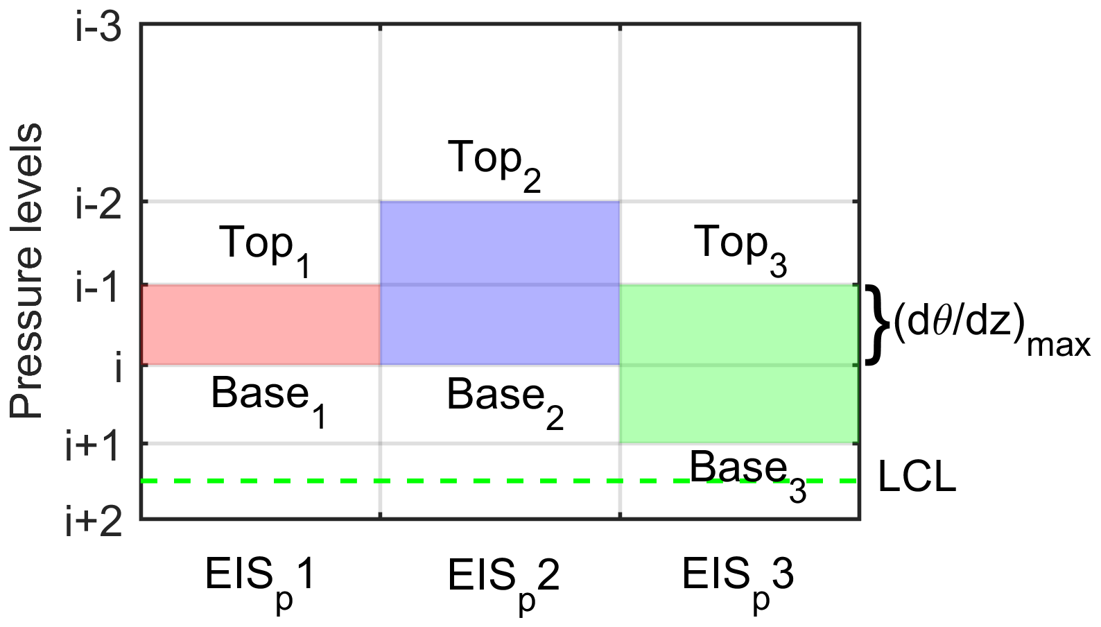
Figure 1An illustration of finding the location of three possible layers encompassing the inversion between the LCL and 5 km a.g.l. in ERA5 or coarse sounding profiles. The red block is one single layer of that includes the inversion. The blue and green blocks are a combination of two adjacent layers if the inversion is distributed into the two layers but not just in the layer of . EISp 1–3 are computed accordingly, and the largest value among them is regarded as the true EISp.
3.1 The algorithm of the new EISp
The EISp is designed to capture the IS information from the thinnest layer encompassing the inversion in low-resolution (hundreds of meters) atmospheric profiles. For these coarse-resolution profiles (e.g., ERA5), it is difficult to accurately locate the exact place of the inversion because, usually, the thickness of the inversion is much smaller than the distance between two adjacent vertical levels. Thus, only one or two adjacent layers that could encompass the inversion are located. The latter is for the consideration that an inversion layer may be across two adjacent layers of the ERA5. Specifically, the EISp is computed as follows:
-
Locating the layer of the maximum θ vertical gradient .
For each hourly ERA5 profile, the layer of is firstly located between the LCL and 5 km a.g.l. (the red zone in Fig. 1), since the inversion only features strong gradients in thermodynamical properties.
-
Finding the layers encompassing the full inversion.
The layer of may not encompass the full inversion if the inversion crosses two adjacent layers of the ERA5. Thus, the layer of is combined with an adjacent layer just above and below it, respectively, to constitute another two candidate layers that could encompass the full inversion (the blue and green zones in Fig. 1).
-
Calculating the EISp.
The EISp is calculated for the three possible layers identified in the second stage, respectively:
where subscripts “top” and “base” represent the top and base levels of a candidate layer. Γm is computed using Eq. (5) at the base level. The θ increase of the moist adiabat is removed to extract the strength of the inversion between the top and base levels, which is consistent with the EIS framework in Wood and Bretherton (2006). The final EISp is determined by which layer in Fig. 1 encompasses the stronger inversion computed from Eq. (8) and thus refers to the largest value among the three candidates EISp 1–3.
The EIS (Wood and Bretherton, 2006) assumes that the PBL is well mixed (dry adiabat below the LCL and moist adiabat above the LCL) for estimating the IS. If that is the case, EISp would give the same results as EIS. However, it will be shown in the following sections that the actual PBL often deviates from the well-mixed conditions, where the EISp provides a physically more reasonable estimate for the IS than the EIS and thus a stronger cloud-controlling factor.
When high-resolution radiosondes are available, the exact IS can be obtained fairly straightforwardly (Sect. 2.5, Eq. 6). The computation of EISp is in fact adapted from the algorithm for obtaining the IS from high-resolution radiosondes but is adjusted to suit coarse-resolution atmospheric profiles in reanalysis. Because high-resolution soundings are rare, an applicable metric derived from reanalysis would be much more beneficial. Because the IGRA soundings have similar vertical resolutions as ERA5 in the lower troposphere, the IS of these soundings (used in Sect. 3.3) is derived in exactly the same way as the EISp.
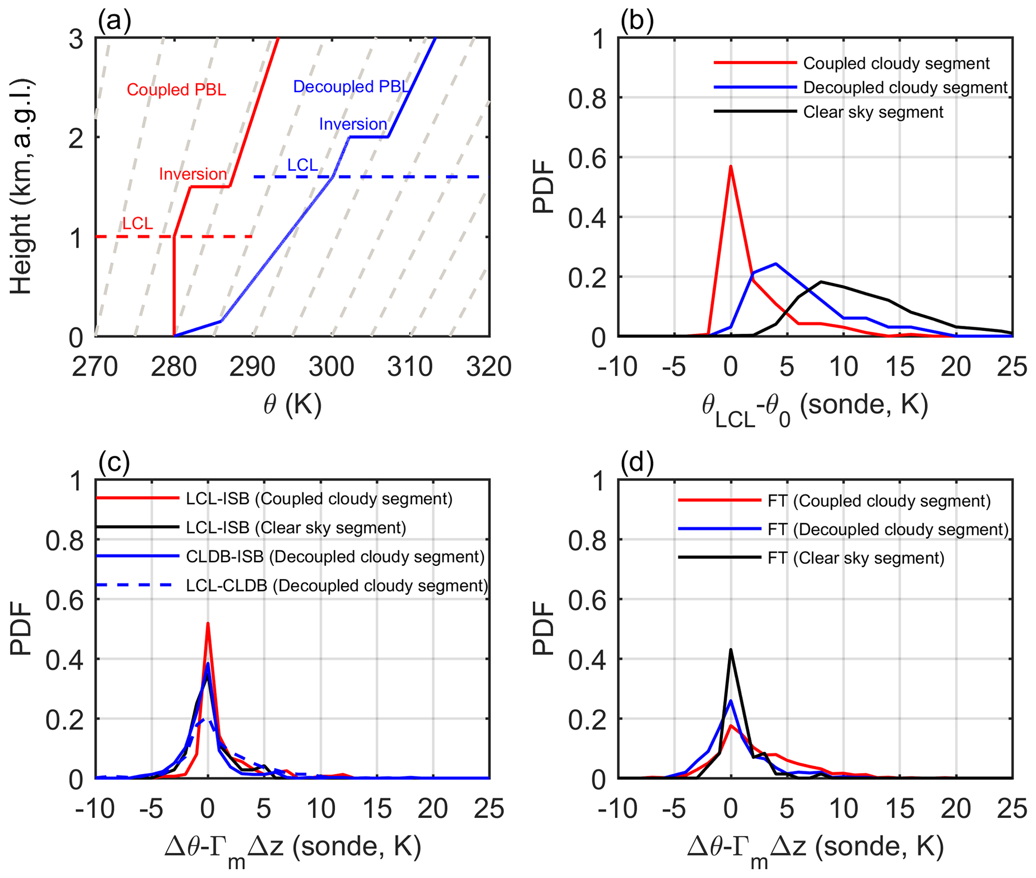
Figure 2Illustrations of PBL θ profiles (a), with the LCL heights indicated by dashed horizontal lines and the moist adiabat represented by light dashed lines. PDFs of the θ difference between the LCL and 150 m a.g.l. (b), the θ difference with the moist adiabat removed between the LCL and the inversion base (c), and the θ difference with the moist adiabat removed for the free troposphere between the inversion top and 3 km a.g.l. (d). The red, blue and black lines are for coupled cloudy, decoupled cloudy and clear-sky segments, respectively. In (c), the θ differences of decoupled cloudy segments are further separated into those between the LCL and the cloud base (dashed blue line) and those between the cloud base and the inversion base (solid blue line).
3.2 PBL stratification and the establishment of the EISp at the SGP
The characteristics of PBL thermal structures are examined by using the SGP high-resolution radiosondes as shown in Fig. 2. Figure 2a illustrates an idealized θ profile of the well-mixed condition consistent with Wood and Bretherton (2006) and an idealized θ profile of the decoupled PBLs based on the observations in Jones et al. (2011). The primary difference in the θ profiles between the coupled and decoupled PBLs is whether a stable layer exists to decouple the cloud and subcloud layers (Nicholls, 1984). Hence, under the decoupled conditions, the LTS and EIS would include the sum of the PBL IS and the θ increase from the ground to the LCL (the blue line in Fig. 2a). The LTS and EIS can be separated into different terms:
The subscripts of “3 km”, “0” and “LCL” indicate the levels of 3 km, 150 m a.g.l. and LCL. If over oceans, the levels of 3 km and 150 m can be replaced with 700 and 1000 hPa. In Eq. (9a), the LTS can be regarded as the sum of the θ difference between the LCL and 150 m a.g.l. (θLCL−θ0), the θ increase (Δθ) due to the actual θ gradient above the LCL, and the PBL IS. Similarly, in Eq. (9b), the EIS is similar to the LTS, except for the fact that the θ increase due to the moist adiabat (ΓmΔz) above the LCL is removed. It can be seen that the first two terms on the right-hand side of Eq. (9a) and (9b) contribute to the LTS and EIS even though they are not a part of the IS. In the well-mixed PBLs, the two terms θLCL−θ0 and Δθ−ΓmΔz are both equal to zero. Thus, the EIS defined by Eq. (9b) is exactly the IS, and the LTS defined by Eq. (9a) is equal to IS+ΓmΔz under perfectly well-mixed conditions.
At the SGP site, 29 %, 32 % and 39 % observational samples are classified into the coupled cloudy, decoupled cloudy and clear-sky segments, respectively. Note that the Δzb method cannot distinguish whether the PBL is coupled or decoupled when a segment has no low cloud. Thus, the clear-sky segments might contain both coupled and decoupled PBLs. The following is noted about Fig. 2b: (1) the probability distribution functions (PDFs) of θLCL−θ0 for the coupled cloudy segments peak at zero and have relatively positive skewness. The exact reason for the positive skewness is not clear. Because the height of the LCL being close to the simultaneously observed cloud base height is only a necessary condition of a PBL being coupled, a decoupled surface layer and overlaying cloud layer coincidently having the height of an LCL close to the cloud base is not a surprise. Either the advection of clouds from other places or the development of a new surface stable layer while clouds that were formed earlier are still left above might result in positive θLCL−θ0. (2) Strong stratification below the LCL (large positive θLCL−θ0) frequently occurs in the decoupled cloudy and clear-sky segments, with mean values of 6.3 and 11.5 K, respectively. Thus, the non-zero term of θLCL−θ0 will cause LTS and EIS to largely deviate from the real value of IS in the decoupled cloudy and clear-sky segments.
Besides, a premise of using LTS and EIS to measure the IS is that the lower-tropospheric θ gradient can be predicted by the moist adiabat above the LCL. This moist adiabatic assumption is supported in previous studies but still with some uncertainties on the daily timescales (Stone, 1972; Wood and Bretherton, 2006; Schneider and O'Gorman, 2008). According to PDFs of the θ difference between the LCL and inversion base or between the inversion top and 3 km a.g.l. with the moist adiabat removed (Δθ−ΓmΔz), θ likely follows the moist adiabat above the LCL (Fig. 2c and d), with a peak at zero, but all PDFs of Δθ−ΓmΔz have broad distributions. The standard deviation of Δθ−ΓmΔz above the LCL is about 4 K. Note that, here, the Γm is computed using Eq. (5) but is based on the temperature and pressure at the base level of each layer.
Typically, the real IS is less than 10 K. Thus, the term θLCL−θ0 in Eq. (9a) and (9b) will cause a strong overestimation of the IS by the LTS and EIS. Furthermore, the variation of the LTS and EIS is attributed not only to variations of IS but also to variations of the systematical deviations of temperature profiles from the dry adiabat below the LCL. As a result, at the SGP site, the decoupled cloudy and clear-sky segments (with weak IS but large θLCL−θ0) are mixed with the coupled cloudy segments with strong IS when using the LTS and EIS to sort data. Large values of LTS and EIS correspond not only to strong IS but also to weak IS with strong stratification below the LCL. On short timescales (like the daily scale), the spread of Δθ−ΓmΔz (Fig. 2c and d) resulting from the θ gradient deviating from the moist adiabat above the LCL could add additional uncertainty into the LTS and EIS. Hence, weak and even unphysical relationships of clouds and moisture with the LTS and EIS might exist.

Figure 3(a–c) LCC composites of the coupled cloudy (red line) and decoupled cloudy segments (blue line) and the occurrence frequency of the clear-sky segments (black line). (d–f) Composited RH profiles. Composites are based on the SGP radiosonde-measured LTS (a and d), EIS (b, and e) and IS (c and f), respectively. Error bars in (a–c) show the 95 % confidence interval of the mean based on the t test. The solid and dashed black lines in (d–f) indicate the average height of the inversion center and the LCL, respectively. All composites are based on daily data of all seasons for the full period at the SGP.
Figure 3a–c shows that the composited LCCs of cloudy segments are all positively proportional to the radiosonde-measured LTS, EIS and IS. However, the composites of LCC are slightly (significantly) more sensitive to the changes of IS than the changes of LTS (EIS). The occurrence frequency of the clear-sky segments (the number of clear-sky segments divided by the number of total segments) is investigated separately. Figure 3c shows that clear-sky segments are rarely observed when the IS is very strong (∼0 % at 10 K) and more frequently exist with weaker IS (60 % at 0 K). This is consistent with the fact that stronger IS inhibits the entrainment of dry air from the free troposphere and thus favors the formation and maintenance of low clouds and corresponds to less occurrence of the clear sky. On the contrary, such a physically reasonable expectation is not seen (even qualitatively) in the composites of the clear-sky segments based on the LTS and EIS. Figure 3a–b shows that the occurrence frequency of clear-sky segments changes little (even increases) with increasing LTS (EIS). This is also expected based on Fig. 2b showing the existence of a large positive skewness in the term θLCL−θ0 in the clear-sky segments. This strong static stability below the LCL results in large LTS and EIS, even when the real IS is weak.
Composited moisture distribution shows information that is consistent with the LCC composites. Figure 3f shows that the composited RH has an increasing trend towards stronger IS, and high values of RH (RH>80 %) are restricted below 1 km a.g.l. at the large IS value bins. However, the composited RH distribution is completely reversed when sorted by the EIS, with high (low) RH being related to weak (strong) EIS (Fig. 3d). The RH distribution sorted by the LTS has a similar dependence on the magnitude of the LTS (Fig. 3c) as the IS does, but with weaker variations and smaller PBL RH as compared to the composites based on the IS (Fig. 3e). Thus, respectively, the LTS and EIS poorly and incorrectly represent the IS at the SGP site; hence, the dependence of the PBL moisture conditions and LCC on the IS are weakly and erroneously reproduced by the LTS and EIS.
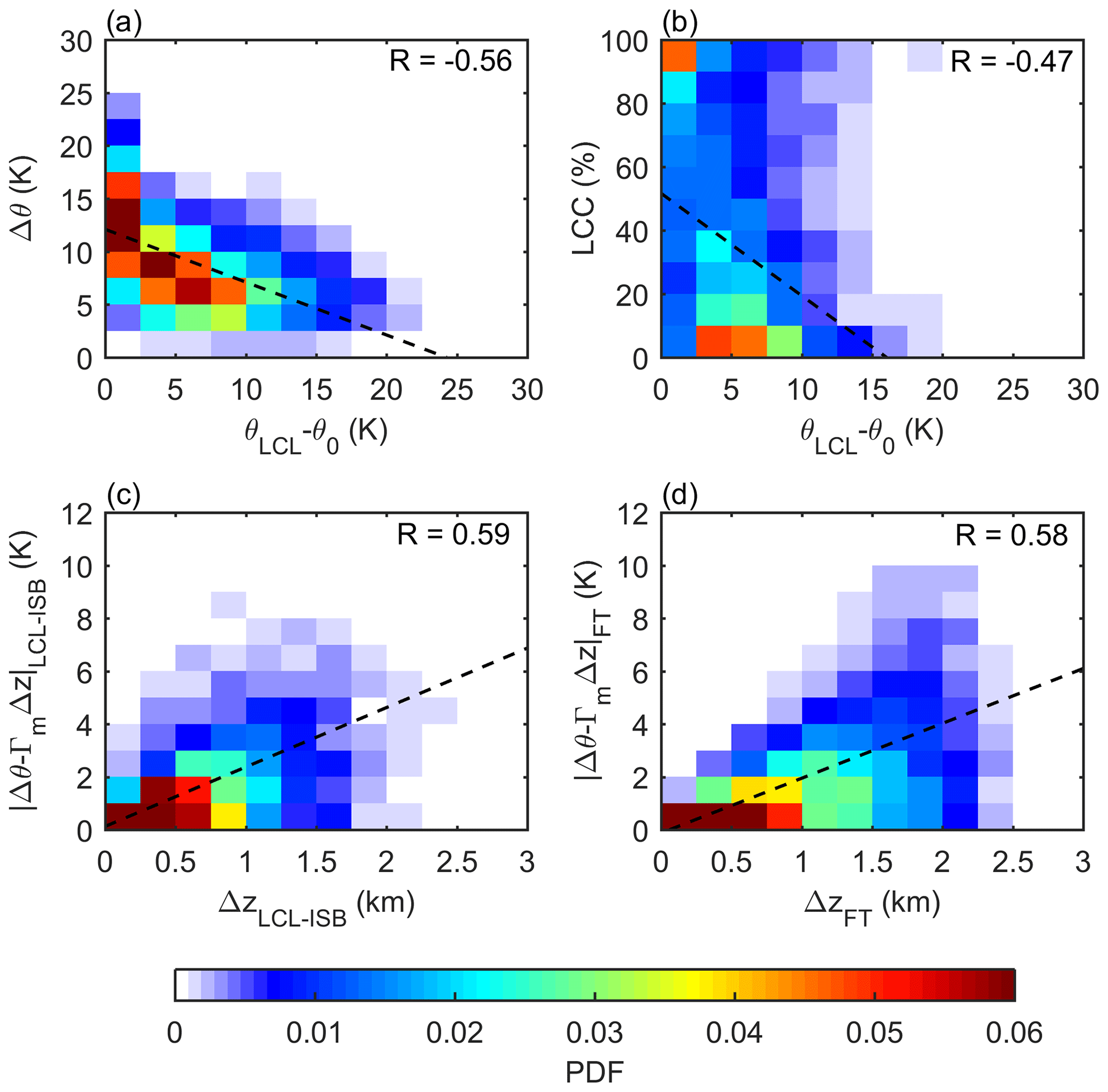
Figure 4Joint PDFs of the θ difference (Δθ) between the levels of 3 km and the LCL (with the IS excluded) and θLCL−θ0 (a), and PDFs of LCC and θLCL−θ0 (b). Joint PDFs of the absolute value of the θ difference with the moist adiabat removed (Δθ−ΓmΔz) and the height difference (Δz) from the LCL to the inversion base (c) and from the inversion top to 3 km in the free troposphere (d). Correlation coefficients (R) are listed in the upper-right corner of each panel. The dashed black lines indicate the least-squares fit.
An interesting phenomenon is that the LTS overall performs better than the EIS with respect to constraining LCC at the SGP site. To understand why this happens, the LTS and EIS in Eq. (9) both have been separated into three terms to discuss. For the LTS, the two terms θLCL−θ0 and Δθ of Eq. (9a) usually offset each other, with a negative correlation of −0.56 and a slope of the least-squares fit of −0.5 K K−1 (Fig. 4a). In contrast, the slope of the least-squares fit between Δθ−ΓmΔz and θLCL−θ0 is only −0.05 K K−1 (not shown). Furthermore, the LTS and EIS equation can be transformed into the following:
On average, the coefficient before θLCL−θ0 for the LTS in Eq. (10a) is 0.5, while that for EIS in Eq. (10b) is 0.95. The variations of LTS and EIS result from both the changes of IS (positively correlated with LCC, as shown in Fig. 3c) and the changes of θLCL−θ0 (negatively correlated with LCC, as shown in Fig. 4b). According to Eq. (10a) and (10b), the LTS actually only involves half of the bias caused by θLCL−θ0 and is thus not as strongly influenced by θLCL−θ0 as the EIS. As a result, removing only the moist adiabat (ΓmΔz) does not make the EIS a better estimate for the IS at the SGP but instead makes the EIS more influenced by θLCL−θ0. This explains why the LTS is better correlated with LCC and RH (Fig. 3a and d) than the EIS (Fig. 3b and e) at the SGP. However, the physical reason why the PBL stratification changes in this way is unclear to us, and it is beyond the scope of this study.
As shown in Fig. 2c and d, the θ difference between the actual environmental θ gradient and the moist adiabatic θ gradient (Δθ−ΓmΔz) is another source of uncertainty in the EIS based on Eq. (9b), especially on short timescales. However, Fig. 4c and d suggest that the spread of increases with the layer thickness, either between the LCL and the inversion base or between the inversion top and 3 km a.g.l. (with a correlation of 0.59 or 0.58, respectively). Thus, the thicker the layer encompassing inversion involved in the EIS calculation is, the larger the uncertainty is. Including more layers around the inversion layer in estimating the IS likely results in more uncertainty. This suggests a possible way of better estimating the IS if we can reduce the layer thickness (Δz) associated with the second term on the right-hand side of Eq. (9b), which also makes the IS estimate less dependent on the moist adiabatic assumption.
The above results suggest that there are two major bias and error sources when estimating the IS using the LTS and EIS metrics. One is caused by systematic deviations from the dry adiabat below the LCL, and the other is the errors resulting from the spread of the actual θ gradient around the moist adiabat above the LCL. To exclude the former source, we can locate the LCL and only consider the inversion above the LCL to drop the first term on the right-hand side of Eq. (9b). The impact of the latter one can be indirectly reduced by finding the thinnest layer encompassing the inversion that is involved in the computation of the second term on the right-hand side of Eq. (9b). Thus, the new EISp (as described in Sect. 3.1) is proposed accordingly to achieve a better estimate of the IS.
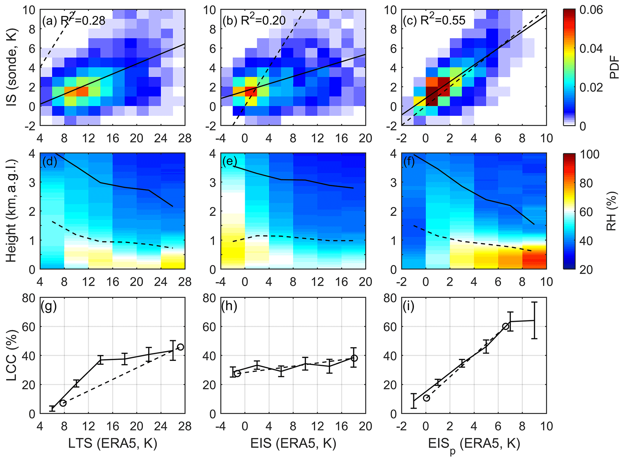
Figure 5Joint PDFs of the SGP radiosonde-measured IS and the ERA5-derived LTS (a), EIS (b) and EISp (c), respectively. In (a–c), the solid black line is the least-squares fit, and the dashed line is the reference line of y=x. The composites of the radiosonde RH profiles based on the ERA5-derived LTS (d), EIS (e) and EISp (f). The solid black and dashed lines in (d–f) are the heights of the IS and the LCL, respectively. The LCCs composited based on the LTS, EIS and EISp are shown in (g–i), respectively. The cycles in (g–i) correspond to the 5 % and 95 % quantiles of LTS, EIS and EISp and the composited value of LCC in the bins of the smallest and largest 10 % of LTS, EIS and EISp values. Error bars in (g–i) show the 95 % confidence interval of the mean based on the t test.
The LTS, EIS and EISp derived from the hourly ERA5 reanalysis are directly compared against the SGP radiosonde-measured IS. In Fig. 5c, the R square between the EISp estimated from the ERA5 and the IS measured by radiosondes is 0.55, which is much larger than those of the LTS (0.28, Fig. 5a) and EIS (0.20, Fig. 5b). The slope of the least-squares fit of the IS to the EISp is 0.86 K K−1. This indicates that the value of the EISp is much closer to the IS as compared to the LTS (0.26 K K−1) and EIS (0.19 K K−1). The composites of LCC and RH based on the EISp (Fig. 5f) show similar results to that based on the IS (Fig. 3f). Stronger EISp corresponds to larger RH trapped below about 1 km, and with the EISp weakening and the inversion layer lifting, RH decreases but distributes to higher levels. However, the LCC and RH composites based on the LTS and EIS (Fig. 5d, e, g and h) show weak or erroneous relationships similar to the results based on the radiosonde-measured LTS and EIS (Fig. 3a, b, d and e). Thus, the EISp offers a better fit to the real IS and better constrains the PBL moisture distribution and LCC. The slope of the composited LCC to the EISp is 6 % per kelvin, in contrast to that of the LTS (1.9 % per kelvin) and the EIS (0.4 % per kelvin). Since the ranges of the LTS and EIS are larger than that of the EISp, larger slopes of the LCC to the EISp than those to the LTS and EIS are expected. To measure the sensitivity of LCC to changes of LTS, EIS and EISp, we consider the effective range of LCC resolved by changes in a metric. The sensitivity of LCC to a metric here is defined as the difference between the composited LCC values associated with the largest and smallest 10 % of that metric:
The bar over the LCC head represents the mean value of LCC sorted by x quantile. x90% and x10% are the 90 % and 10 % quantiles of x. The LCC sensitivity of all segments to the EISp is 50 %, which is larger than that to the LTS (39 %) and EIS (12 %). These weaker and erroneous dependences of LCC on the LTS and EIS, respectively, are expected, since large errors (Fig. 2b–d) are carried in the LTS and EIS. Although the vertical resolution of the ERA5 profiles may not always suffice to resolve the inversion layer, the IS estimated from the ERA5 profile-based algorithm (EISp) is highly consistent with the IS directly derived from the SGP 10 m resolution radiosondes, and they present similar relationships with the PBL RH and LCC.
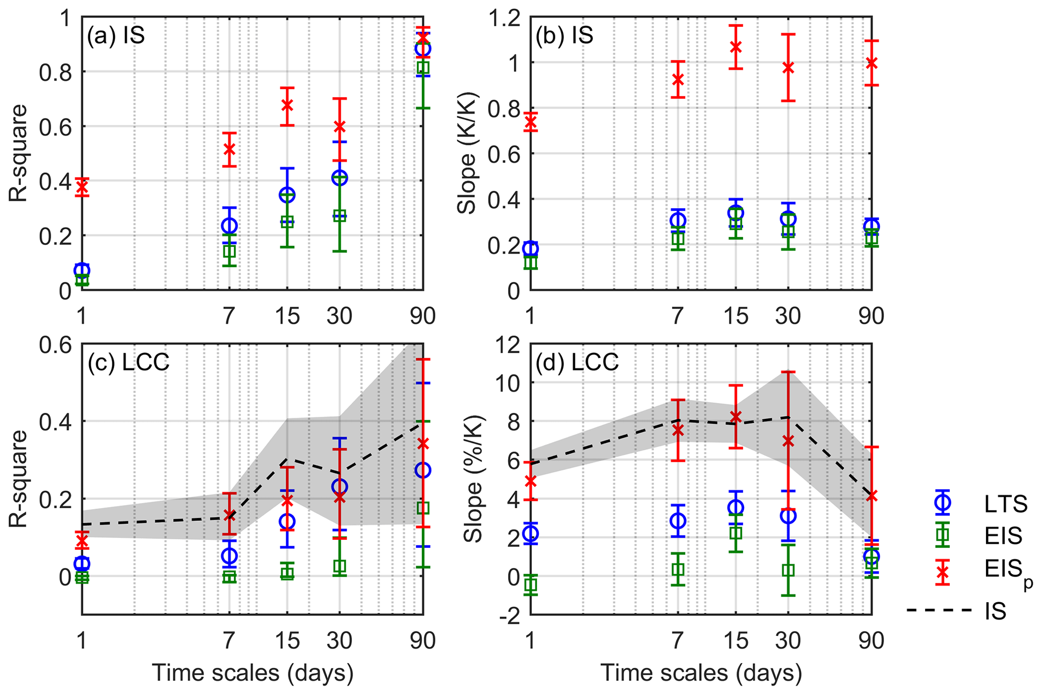
Figure 6R square (a) and slope of the least-squares fit (b) of the SGP radiosonde-derived IS to the ERA5 reanalysis-based LTS (blue cycle), EIS (green square) and EISp (red cross) on daily, 7, 15, 30 and 90 d timescales, respectively. R square (c) and slope (d) of LCC to the LTS, EIS, EISp and IS (dashed black line) on daily to seasonal timescales, respectively. Error bars and shadows show the 95 % confidence interval of the mean based on the t test.
The ERA5-based LTS, EIS and EISp are further examined on the different timescales with respect to their relationships with radiosonde-measured IS and LCC (Fig. 6). Overall, the R square and the slope of the EISp with the IS are the largest throughout all timescales as compared to those of the LTS and EIS. Particularly on the daily, 7 and 15 d timescales, the lower bounds of the 95 % confidence interval of the EISp–IS R square are much higher than the upper bounds for the LTS and EIS. On the seasonal timescale, three metrics have similar correlations with the IS, but as shown in Fig. 6b, the slope of the IS to the EISp (nearly 1) is still much larger than those to the LTS (0.28 K K−1) and EIS (0.23 K K−1). The limited accuracy restricts the LTS and EIS in reproducing the relationship between the true IS and LCC. In Fig. 6c, on daily timescales, the LTS explains 3.1 % of variance in LCC, which is comparable to the 4.8 % variance explained by the LTS at OWS N (a typical low-cloud-dominated site over the ocean) in Klein (1997)). For the EISp, it explains 9.1 % of the daily LCC variance, which is remarkably close to that explained by the IS. Similar conclusions can be drawn from weekly timescales. On longer timescales, the EISp and the LTS both explain comparable variance in LCC but much larger variance than that explained by the EIS. In Fig. 6d, the slope of LCC composited based on the IS is nearly reproduced by the EISp consistently. The slopes of LCC composited based on the LTS and EIS are much smaller than those based on the EISp and IS.
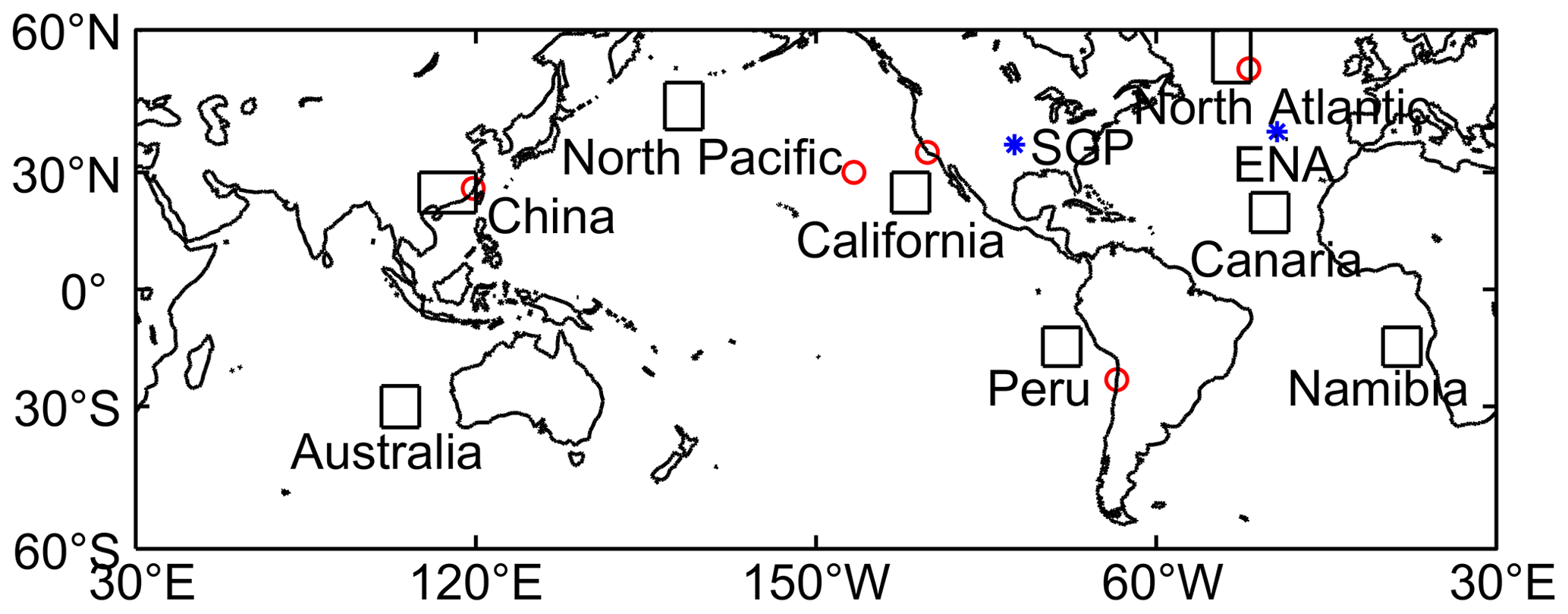
Figure 7Blue asterisk marks the SGP and ENA sites. Red cycles mark the locations of radiosonde stations from the IGRA. Eight boxes are the most typical low-cloud-dominated regions defined in Klein and Hartmann (1993).
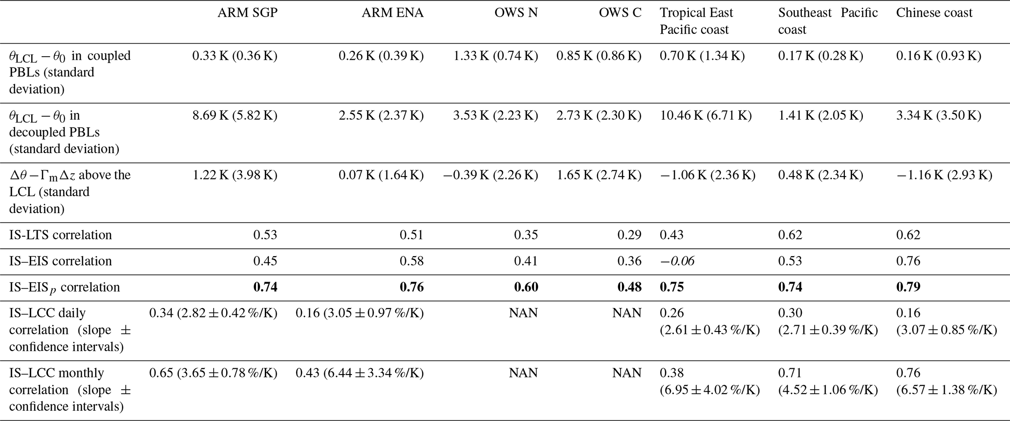
Table 2The characteristics of the PBL thermal structures and evaluation of the LTS, EIS and EISp in terms of estimating the IS and the IS–LCC relationships of the six radiosonde stations. Coupled and decoupled PBLs of all stations are distinguished by αθ. Italics indicate not-significant correlations. Bold indicates the largest correlation. The daily IS–LCC correlation is based on the data after subtracting 7 d means.
3.3 Validation of the EISp at radiosonde stations of the subtropics and midlatitudes
As shown in Sect. 3.2, at the ARM SGP site, the EISp estimates the PBL IS better than both the LTS and EIS when the PBL thermal structure is largely deviated from the idealized structure of well-mixed PBLs. Next, we want to see if such a deviation exists at other radiosonde stations of the subtropics and midlatitudes. The ARM ENA site and another five ground-based radiosonde stations are selected to examine their characteristics of PBL thermal structures. Their locations are shown in Fig. 7. Because the cloud base height information is not available at the radiosonde stations of IGRA, the method used at the SGP to distinguish the coupled cloudy, decoupled cloudy and clear-sky segments is not accessible. Thus, an alternative indicator, the decoupling degree (αθ), is used to distinguish coupled and decoupled PBL according to the PBL thermal structures. The definition of αθ is introduced in Wood and Bretherton (2004) by using the liquid potential temperature (θL) as the conserved variable during the moist adiabat. Here, θ is used to construct the moist adiabatic conserved variable by removing the moist adiabatic θ increase above the LCL to express the αθ parameter:
The subscripts “ISB”, “IST”, “0”, “700 hPa” and “LCL” indicate the base and top of the inversion layers, the levels of 1000 and 700 hPa, and the LCL, respectively. To understand its meaning, Eq. (12) can be transformed as follows:
The numerator of αθ can be understood as the strength of the PBL thermal structures deviating from the coupled conditions. The denominator of αθ can be understood as the sum of the deviation strength of the PBL thermal structure from the coupled conditions and the IS (or EIS). By Eq. (13), the EIS can also be expressed as IS. Thus, whether the EIS is the real IS is actually determined by the decoupling parameter αθ. In perfectly coupled conditions, αθ is zero and the EIS is exactly equal to the IS. In decoupled PBLs, when αθ is larger, the EIS actually accounts more for the deviation of the PBL thermal structure from the coupled condition. A small value of αθ would suggest a state very close to the coupled condition, and here, a threshold value of 0.2 is used to distinguish the coupled and decoupled PBLs based on Eq. (12). αθ has been tested for the high-resolution soundings, and it comes to similar results. In fact, results listed in Table 2 at the SGP based on αθ show consistent results with that based on Δzb.
As shown in Table 2, it is found that the two terms θLCL−θ0 and Δθ−ΓmΔz in Eq. (9) are non-negligible, even over the subtropical oceans. Both the mean and standard deviation of θLCL−θ0 are very small in the coupled PBLs. The mean of θLCL−θ0 at the other sites in the decoupled PBLs is usually smaller (about 1–4 K) as compared to that at the SGP (8.69 K), except at the tropical East Pacific coast, where it is larger (10.46 K) than that at the SGP. Theoretically, a constant shift on the θ difference between the LCL and the ground level will not change the correlation coefficient and regression slope between the LTS and EIS and the IS and LCC. However, the term θLCL−θ0 is systematically different between the coupled and decoupled PBLs. Thus, using the LTS and EIS to sort the PBL structures will unequally mix the coupled and decoupled conditions in their different composite bins. Moreover, this bias is distinct for different places, and thus, the regional difference would make the LTS and EIS not uniform in terms of their accuracies when estimating the IS. In contrast, this will not happen in the EISp, since this bias caused by the term θLCL−θ0 in the LTS and EIS is completely excluded from the EISp.
The standard deviation of the term Δθ−ΓmΔz, as shown in Table 2, suggests that the errors in estimating the IS based on Eq. (9) due to the moist adiabatic assumption above the LCL of the ENA and the other five radiosonde sites range from 57 %–74 % of that of the SGP site (3.98 K). Thus, the term Δθ−ΓmΔz at these six sites will likely also be reduced when measuring the IS by the EISp. Thus, it is not surprising that the ERA5 EISp is best correlated with the IS directly derived from the radiosondes over all stations (Table 2). Regional differences of the correlations with the IS still exist for all metrics to measure the IS but are relatively small for the EISp.
In this section, the relationship of global LCC with LTS, EIS and EISp is discussed through daily to seasonal timescales. Since ground-based observations of radiosondes from ARM and IGRA are all assimilated in the ERA5 reanalysis (Hersbach et al., 2020), it is not surprising that the assimilated output can capture well the PBL thermal structures to estimate the IS for these locations where ground-based observations are available. However, for most areas of the oceans, only limited radiosondes are available over scattered islands or during short-term campaigns of field experiments to be used in ERA5 assimilation, and thus, whether the IS can be rightly captured from the ERA5 profiles needs further examination. In this section, whether the EISp derived from the ERA5 profiles at the global scale (especially for oceans with few radiosondes assimilated into the ERA5) can better constrain LCC than LTS and EIS is explored.
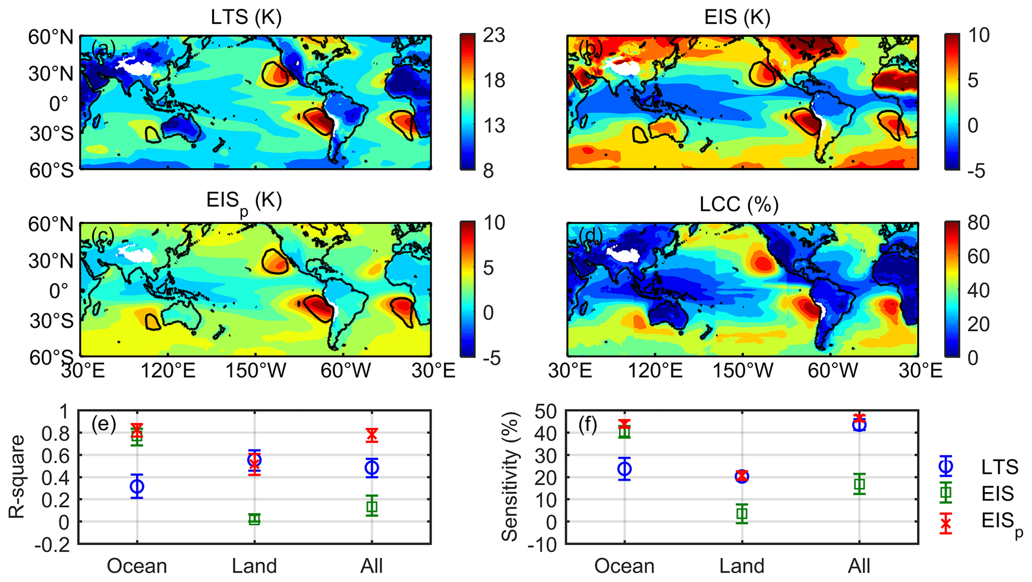
Figure 8Spatial distribution of the ERA5 reanalysis-based LTS (a), EIS (b), EISp (c) and the GEO-MODIS LCC (d) between 60∘ S and 60∘ N. The black contours enclose regions with LCC larger than 60 %. The specific R square and LCC sensitivity to the LTS (blue cycle), EIS (green square) and EISp (red cross) over the ocean, land and all is shown in (e) and (f), respectively. The error bars show the 95 % confidence interval of the mean based on the t test.
Figure 8 shows the 6-year mean map of the ERA5-based LTS, EIS and EISp. The GEO-MODIS LCC global pattern is also used to examine its spatial correlation with the above three metrics. For the LTS, EIS and EISp, the plateau regions with surface pressures smaller than 700 hPa are not investigated here, where no GEO-MODIS LCC is observed. Overall, the annual mean values of LTS and EIS are obviously larger than the EISp value, except in the inner tropical convective zone, where the EIS value is largely negative. In addition, there are three differences between the spatial distributions of LTS, EIS and EISp.
-
Over the subtropical eastern oceans, the center locations of LTS, EIS and EISp are different. For LTS and EIS, their center locations are more eastward and adjacent to the coast as compared with the center locations of EISp and LCC. For EISp, its center locations are relatively far away from the coast and more consistent with the center locations of LCC.
-
Over midlatitude oceans, the contrast of the values between the midlatitudes and the tropics is different for LTS, EIS and EISp. The midlatitude LTS reduces to the minimum but still corresponds to about 40 % of LCC. The midlatitude EIS is as strong as the EIS over the subtropical eastern oceans but corresponds to a much smaller LCC than the subtropical LCC. Only the variation of EISp from the tropics to midlatitudes is more reasonably consistent with the spatial variation of LCC.
-
Over land, the LTS and EISp explain over half of the LCC spatial variance according to their linear fit, but the EIS only explains 2 % of the LCC spatial variance. This implies that the IS is still a controlling factor for LCC distribution over land. The EIS barely correlates to continental LCC, possibly because the EIS poorly estimates IS due to the strong influence of the term θLCL−θ0, as discussed in Sect. 3.
On the whole, the performance of EISp is better and less dependent on surface types. Over all global oceans and land, the EISp explains 78 % of the spatial variance in LCC, which is significantly higher than that explained by the LTS (48 %) and the EIS (13 %). The spatial variations of LCC are also more sensitive to the EISp (Fig. 8f).
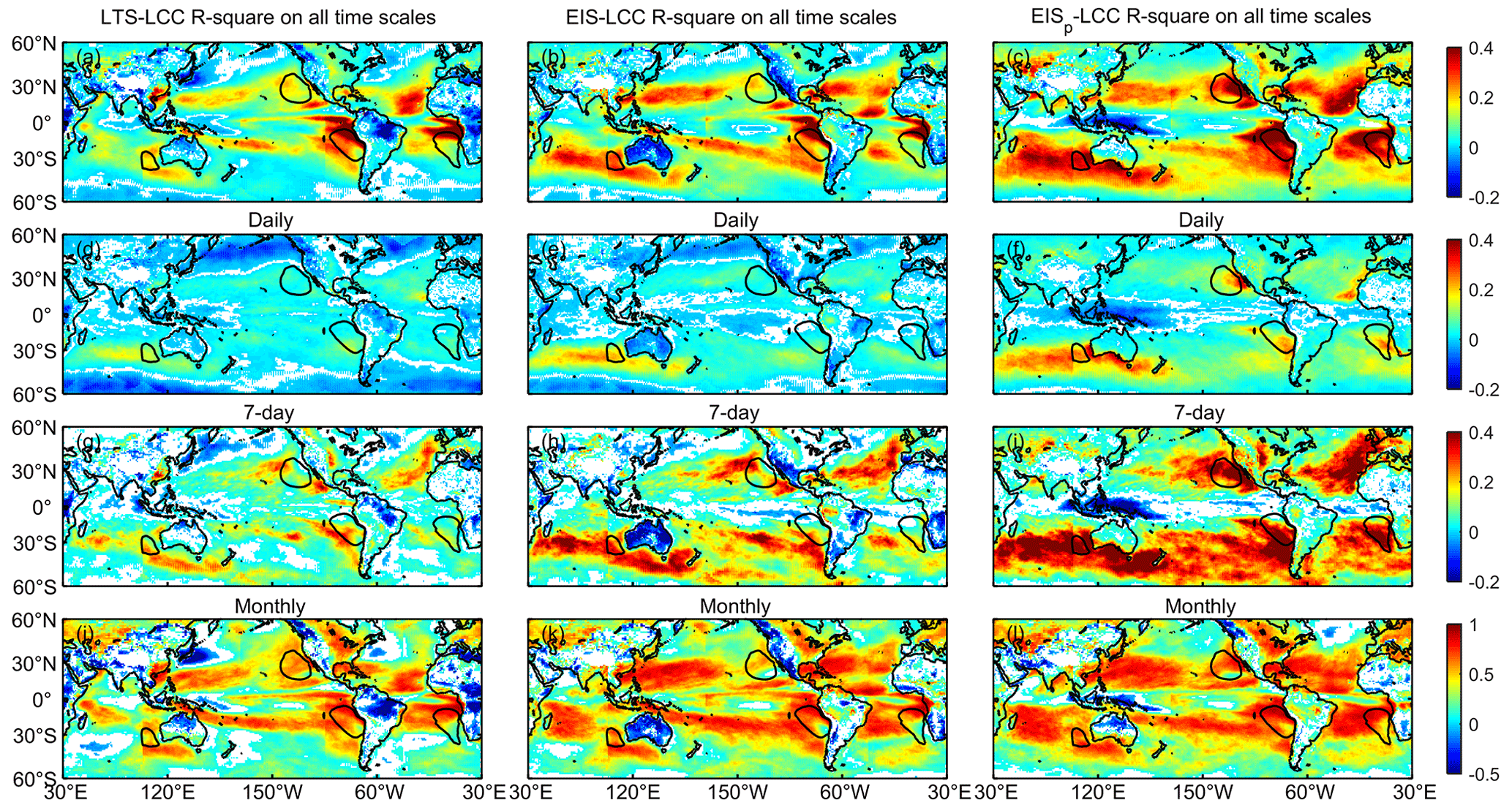
Figure 9R square between the GEO-MODIS LCC and the ERA5 reanalysis-based LTS (left column), EIS (middle column) and EISp (right column) at the all timescales (a–c), daily timescale (d–f), 7 d timescale (g–i) and monthly time scale (j–l). The black contours enclose regions with LCC larger than 60 %. Only R squares at the 95 % significance level are shown. The minus (plus) sign of R square indicates negative (positive) correlations.
In Fig. 9, the dependence of LCC on the LTS, EIS and EISp is further examined globally for the full daily time series (i.e., all timescales) and for the daily, 7 d window-averaged anomalies and monthly means (i.e., daily, 7 d and monthly timescales). It is noted that the dependence of LCC on the three ERA5-based metrics varies across different regions. LCC is best correlated with three metrics over the subtropical eastern oceans and some land regions that are most dominated by low clouds. Over midlatitude oceans and the inner Tropical Convergence Zone, the LCC is weakly or negatively correlated with three metrics. Thus, it is discussed separately for the most LCC-dominated regions over subtropical oceans, midlatitude oceans and land.
-
Over the subtropical eastern oceans with more than 60 % of LCC, on all timescales (Fig. 9a–c), the EISp explains 36 % of the variance in LCC on average, which is larger than that explained by the LTS (21 %) and the EIS (20 %). The fact that EIS does not provide a stronger correlation with LCC than LTS was also recognized by Park and Shin (2019) and by Cutler et al. (2022). In contrast, the explained variance of the linear fitting between LCC and EISp is 1.8 times that with LTS and EIS. Besides, the mean LCC sensitivity (defined in Eq. 11 and not shown in the figure) to the EISp on all timescales is 48 % over these regions, which is significantly higher than that to the LTS (37 %) and the EIS (36 %). Although radiosondes are rare and the ERA5 profiles are mostly from the model output over these regions, the EISp still provides a much stronger constraint on LCC than LTS and EIS. As shown in Fig. 9d–i through daily to monthly timescales, the EISp robustly explains larger LCC variance, more so than the LTS and EIS, especially on short timescales.
-
Over midlatitude oceans, weak and not-significant correlations between LCC and the three metrics exist through all of the timescales in Fig. 9. This poor relationship is also found at the ENA site (Table 2), even when using the radiosonde to derive the IS, and thus, it is not caused by using the ERA5 to estimate the IS. This suggests that the IS–LCC relationship is indeed not uniform but varies with regions. Klein et al. (2017) also indicated that the LCC relationship with cloud-controlling factors (e.g., the IS and sea surface temperature) is systematically different between the subtropical stratocumulus region and other regions (e.g., trade cumulus and midlatitude regions). Thus, when the IS is used to constrain the environmental influence on LCC variations, it should be noted that LCC is not all uniformly constrained by the IS for different regions. For some regions such as midlatitude oceans, the IS might not be a good constraint on LCC. But by more accurately estimating the IS, the EISp is more correlated with LCC than the LTS and EIS over midlatitude oceans such as the North Pacific and North Atlantic on all timescales in Fig. 9a–c.
-
Over land regions of relatively more LCC (about 15 %–25 % in South America, China and Europe), the correlation between EISp and LCC is comparable to the subtropical oceanic regions through all of the timescales in Fig. 9. This suggests that the EISp is also an important controlling factor for continental LCC over these regions. Besides, the EISp is more correlated with LCC than the LTS and EIS over most land regions, except over China, where the LTS explains larger LCC variance than the EIS and EISp. The higher correlation of LTS with LCC over China might not be attributed only to the IS (LTS is not a direct measure of inversion but static stability). But more comprehensive and in-depth investigations on the LTS–LCC dependence are needed to understand the exact reason for this phenomenon.

Figure 10R square (left panel), slope (middle panel) and relative sensitivity (right panel) of the GEO-MODIS LCC to the ERA5-based regional mean LTS (blue cycle), EIS (green square) and EISp (red cross) through daily to seasonal timescales over the five typical eastern oceans defined in Klein and Hartmann (1993). The error bars show the 95 % confidence interval based on the t test. The dashed black lines in the left panel are the fraction of the LCC variance on different timescales divided by the total variance.
In Klein and Hartmann (1993), several key low-cloud regions are defined. Those regions are of a particular interest in climate projections due to their strong low cloud albedo effects. As shown in Fig. 7, we pick eight key low-cloud regions according to Klein and Hartmann (1993), and the linear relationships between LCC and the three metrics are investigated. These regions lack radiosondes for long-term observations of IS. They are separated into a group of five typical tropical and subtropical low-cloud-prevailing eastern oceans (Fig. 10) and a group of midlatitude oceans and subtropical land (Fig. 11).
As shown in Fig. 10 (the dashed line in the left panel), over the five key tropical and subtropical eastern oceans, the daily and seasonal window-averaged LCC anomalies account for a larger portion of the total LCC variance, indicating that the LCC variation mainly happens at the daily and seasonal timescales. Over the Peruvian, Namibian and Canarian regions, over 50 % of LCC variances are from the seasonal variations, and much smaller LCC variances are from other four shorter timescales. But over the Californian and Australian regions, 40 % and 51 % of the LCC variances are from the daily timescale, which are larger than those on other timescales. Although the LCC variances on the 7 d, 15 d and monthly timescales are relatively smaller, the sum of them still accounts for about 20 % ∼ 30 % of the total LCC variance.
In Fig. 10, the LCC variance explained by the LTS, EIS and EISp and the LCC slopes of the linear regression to them are examined through daily to seasonal timescales. In addition, the relative LCC sensitivity to those three metrics refers to the LCC sensitivity as defined in Eq. (11) divided by the LCC range. Here, the LCC range is the difference between the mean values of the largest and the smallest 10 % of LCC. The LCC variance is explained most by the EISp among the three metrics (left panel of Fig. 10), and LCC is most sensitive to the EISp (right panel of Fig. 10) through all of these timescales, except in the cases of the monthly timescale over the Peruvian region and the seasonal timescale over the Namibian region. On the daily timescale, 32 % of LCC variances are explained by the EISp on average over the five eastern oceans, which is more than 2 times the variance explained by the LTS (14 %) and EIS (16 %). On the longer timescales (30–90 d), overall, the EISp explains 89 % of the LCC seasonal variance on average over the five eastern oceans, in contrast to 80 % for the LTS and 70 % for the EIS. Only the EISp can robustly explain the seasonal variance of LCC exceeding 80 % for all locations. However, the EIS cannot explain well the seasonal variation of LCC over the Californian and Canarian regions, and the LTS cannot explain well the seasonal variation of LCC over the Australian region.
It is also noted that the slopes of LCC associated with each metric are not uniform across these key low-cloud regions or on different timescales. A similar regional and temporal difference is also found in the LCC–IS relationships (Table 2). Klein et al. (2017) and Szoeke et al. (2016) also found the LCC slopes to the LTS and EIS are variant on different timescales, and this timescale dependence would lead to uncertainties in the final estimates of low cloud feedbacks. Thus, the error estimates of the LCC slopes to the LTS, EIS and EISp are needed for the final uncertainty estimates of low cloud feedbacks. To quantify the relative variation (or the uniformness) of the LCC slope to LTS, EIS and EISp, we compute the ratio between the standard deviation and the mean of grouped slopes. For the temporal relative variation, slopes on different timescales of each region are grouped together, while for the regional relative variation, on each timescale, slopes over different regions are grouped together. The temporal relative variation of the LCC slope to the LTS and EIS is 32 % and 29 % on average over the five eastern oceans. In contrast, the temporal relative variation of the LCC slope to the EISp is 21 %. Besides, the regional relative variation of the LCC slope to the LTS, EIS and EISp is 24 %, 21 % and 18 % between the five eastern oceans, respectively. This suggests that the regional and temporal dependence of the LCC slope in the estimate of low cloud feedbacks is also non-negligible and needs to be considered in the final error estimates or to estimate low cloud feedbacks by separating regions.
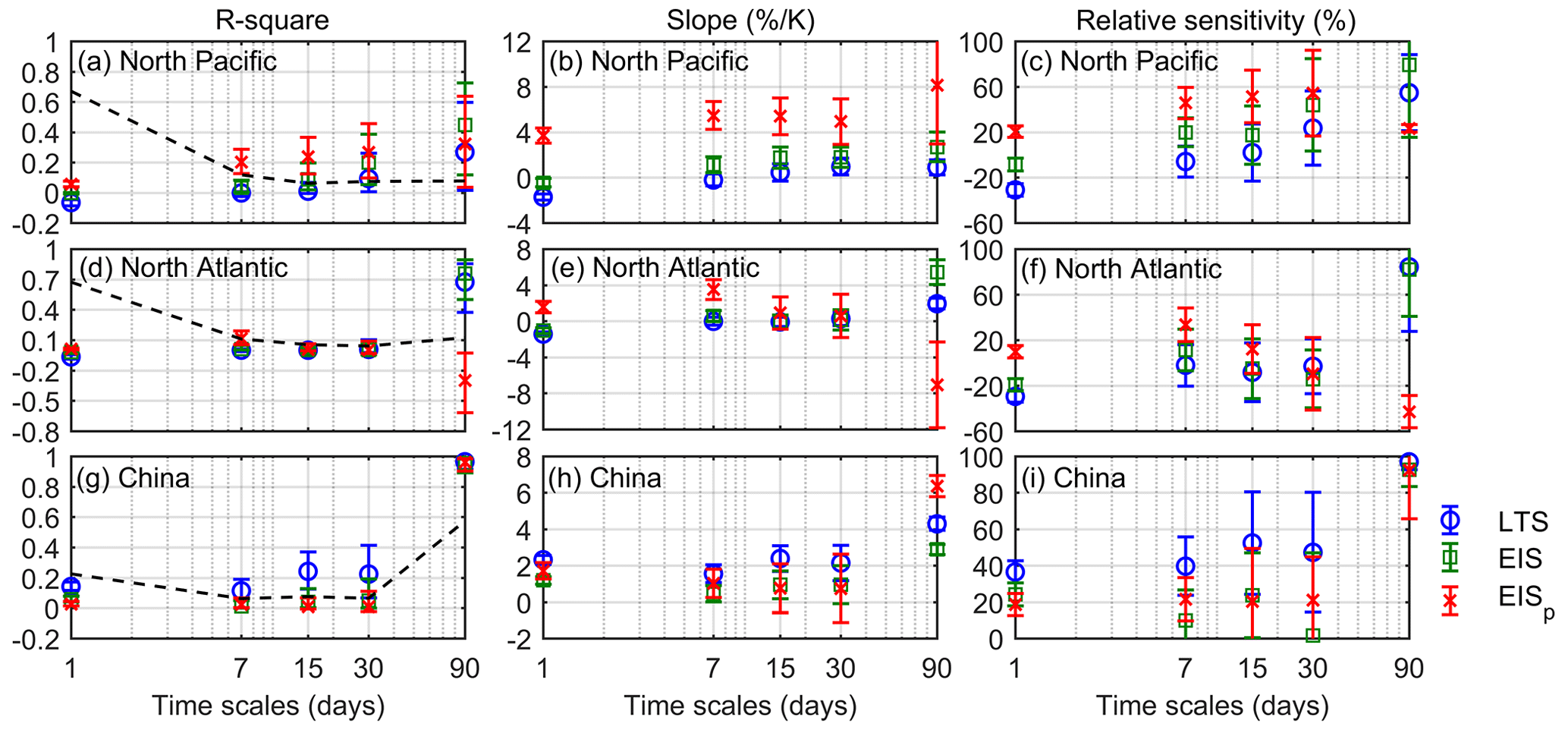
Figure 11Similar to Fig. 10 but for the other three regions defined in Klein and Hartmann (1993), including two midlatitude oceans and one subtropical land. The minus (plus) sign of R square indicates negative (positive) correlations.
Figure 11a and d (the dashed line) show that, over the North Pacific and North Atlantic regions, 67 % of the LCC variance is from the daily timescale, while over the China region in Fig. 11g, variance is mostly from the seasonal timescale (57 %). Over the North Pacific and North Atlantic regions, LCC is not necessarily correlated with the IS. Norris (1998) has found that fogs and bad-weather stratus clouds frequently occur over the midlatitude ocean but with less inversion and poor IS–LCC relationships. Similarly, poor correlations (Fig. 11a and d) and sensitivity (Fig. 11c and f) between LCC and LTS, EIS and EISp are found over the North Pacific and North Atlantic. However, the EISp is closest to the radiosonde-detected IS as compared with the LTS and EIS at the ENA and OWS C, as shown in Table 2. This suggests that the EISp is still a reliable estimation for the IS to represent the true IS–LCC relationship. But the LTS–LCC and EIS–LCC relationships are not necessarily due to the IS influence on LCC. Figure 11a, d, c and f also show that the LTS–LCC and EIS–LCC correlations and sensitivities are very different from those between LCC and EISp on the daily and seasonal timescales. Unfortunately, the midlatitude LCC–IS relationship has not been well explored. The poor EISp–LCC relationship is representative of the fact that the IS cannot be a cloud-controlling factor that is as important as that over subtropical oceans. Over the Chinese region, the EIS and EISp are both better correlated with the IS, as shown in Table 2. Figure 11g and i show that LCC is slightly more correlated with and sensitive to the LTS through all timescales. These higher correlations and sensitivities are not related to the IS, since the LTS correlates the least with the IS. Since the LTS not only includes the IS but actually represents the total static stability from 1000 to 700 hPa to influence the amount and liquid water path of low clouds (Klein and Hartmann, 1993; Kawai and Teixeira, 2010), it may imply that there are other thermal factors in addition to the IS in LTS that contribute to these higher correlations and sensitivities. Overall, it should be noted that the IS may not be a strong cloud-controlling factor over the midlatitude oceans and subtropical land, but EISp is still the best estimation for the IS. The IS is not the only LCC-controlling factor, and other factors (e.g., sea surface temperature, cold advection, free-tropospheric humidity and vertical velocity) are also important for influencing LCC (Myers and Norris, 2013; Klein et al., 2017).
All the above analyses (Figs. 8–11) are based on the daily averaged LTS, EIS and EISp data, which are computed based on the 3 h 1∘ ERA5 atmospheric profiles. Based on the monthly mean atmospheric profiles, over the region of LCC larger than 60 %, the LTS and EIS explain 50 % and 48 % of LCC variance, which is similar to the value of 53 % based on the 3 h ERA5 atmospheric profiles. However, the EISp based on the monthly mean ERA5 profiles explains 49 % of the LCC variance, which is significantly lower than the 65 % based on the 3 h profiles. Thus, for accurately computing the EISp on either short or long timescales, a high temporal resolution of reanalysis data is necessary.
In this paper, a novel profile-based estimated IS (EISp) is developed based on the thinnest possible layer that contains the inversion layer in the ERA5 profiles. By this method, the effects of the static stability below the LCL are completely removed. The errors due to the spread of the environmental θ gradient around the moist adiabat above the LCL are reduced.
At the ARM SGP site, the EISp more accurately estimates the IS, with a correlation of 0.74, than the LTS (0.53) and EIS (0.45). Thus, the EISp reasonably replicates the constraints of IS on the PBL moisture distribution and LCC, while the LTS and EIS respectively have a weak and erroneous relationship with the PBL moisture and LCC. The LCC sensitivity to LTS, EIS and EISp is 39 %, 12 % and 50 %, respectively. On the daily timescale (7 d mean excluded), the variance in LCC explained by the EISp (9.1 %) is more than twice that explained by both the LTS (3.1 %) and EIS (−0.4 %). At the ARM ENA site, the EISp has similar advantages when estimating the IS. At other available oceanic and coastal observation stations, the EISp is still a better estimation for the IS than the LTS and EIS are.
At the global scale, according to the GEO-MODIS LCC observations, the EISp explains the spatial and temporal variations of LCC better than the LTS and EIS do. Over oceans, the EISp distribution is more consistent with the LCC pattern compared with those of the LTS and EIS. The locations of the strongest EISp are consistent with the centers of the largest LCC relatively far away from the coast, while the centers of the strongest LTS and EIS are over the coast. Over the subtropical LCC domains, the LCC sensitivity to the EISp is 48 %, which is larger than that to the LTS (37 %) and EIS (36 %) on all timescales. Furthermore, the increased LCC sensitivity to EISp primarily comes from timescales shorter than a month. Over the typical low-cloud-prevailing eastern oceans, as defined in Klein and Hartmann (1993), the LCC daily variance explained by the EISp is 32 % and twice that explained by the LTS and EIS. Furthermore, the LCC seasonal variance explained by the EISp increases to 89 % as compared with that explained by the LTS (80 %) and EIS (70 %).
No uniform relationship between the LCC and any of the IS, LTS, EIS and EISp is found across timescales or different regions. As compared to the LTS and EIS, the temporal relative variation of the LCC slopes to the EISp is reduced from 32 % and 29 % to 21 %. The regional relative variation of the LCC slope to the EISp is slightly smaller than that of the LTS and EIS. This non-uniform LCC sensitivity to cloud-controlling factors across different regions and timescales suggests that using a single observational multi-linear regression between LCC and cloud-controlling factors to estimate the global low cloud feedbacks is not recommended.
Overall, the EISp is an improved measure of the IS and better constrains LCC, especially on timescales shorter than a month. On short timescales, the enhanced dependence of LCC on the EISp makes the EISp more suitable to resolving process-oriented studies associated with LCC variations. Therefore, the EISp is likely a better constraint to reduce the meteorological covariations to separate the aerosol effects in aerosol–cloud interactions.
The code for determining the EISp of an atmospheric profile can be obtained by request to the authors.
All data used in this study are available online. The ARM SGP and ENA radiosonde and cloud observations were obtained from the ARM Research Facility and are available at https://doi.org/10.5439/1595321 (Ken, 2001) and https://doi.org/10.5439/1333228 (Chen and Xie, 1996). The IGRA radiosondes (Durre et al., 2006, 2018) are available from the NOAA National Centers for Environmental Information at https://www.ncei.noaa.gov/products/weather-balloon/integrated-global-radiosonde-archive (NOAA, 2021). The GEO-MODIS LCC product (Doelling et al., 2013; Doelling et al., 2016; Trepte et al., 2019) is provided by the NASA Langley Research Center at https://doi.org/10.5067/TERRA+AQUA/CERES/SYN1DEG-1HOUR_L3.004A (NASA et al., 2021). The ERA5 reanalysis (Hersbach et al., 2020) used in this study is from the ECMWF and available at https://doi.org/10.24381/cds.bd0915c6 (Copernicus Climate Change Service, 2021).
JY and RW designed the experiments, and ZW carried them out. JY and ZW prepared the first version of the paper with contributions from all co-authors. YC prepared the ERA5 data, and TT inspected some individual profiles and cloud images. All authors verified the final version of the paper.
The contact author has declared that none of the authors has any competing interests.
Publisher’s note: Copernicus Publications remains neutral with regard to jurisdictional claims in published maps and institutional affiliations.
This research has been supported by the NSFC-41875004, the National Key R&D Program of China-2016YFC0202000 and the Jiangsu Collaborative Innovation Center for Climate Change. The first author thanks the “Double First-class” initiative program for providing an opportunity for him to visit the University of Washington. We thank two anonymous referees for their helpful comments.
This research has been supported by the National Natural Science Foundation of China (grant no. 41875004) and the National Key Research and Development Program of China (grant no. 2016YFC0202000).
This paper was edited by Johannes Quaas and reviewed by two anonymous referees.
Ackerman, T. P. and Stokes, G. M.: The Atmospheric Radiation Measurement Program, Physics Today, 56, 38–44, https://doi.org/10.1063/1.1554135, 2003.
Albrecht, B. A., Jensen, M. P., and Syrett, W. J.: Marine boundary layer structure and fractional cloudiness, J. Geophys. Res., 100, 14209–14222, https://doi.org/10.1029/95jd00827, 1995.
Bretherton, C. S. and Wyant, M. C.: Moisture Transport, Lower-Tropospheric Stability, and Decoupling of Cloud-Topped Boundary Layers, J. Atmos. Sci., 54, 148–167, https://doi.org/10.1175/1520-0469(1997)054<0148:Mtltsa>2.0.Co;2, 1997.
Bretherton, C. S., Widmann, M., Dymnikov, V. P., Wallace, J. M., and Bladé, I.: The Effective Number of Spatial Degrees of Freedom of a Time-Varying Field, J. Climate, 12, 1990–2009, https://doi.org/10.1175/1520-0442(1999)012<1990:Tenosd>2.0.Co;2, 1999.
Bretherton, C. S., Uttal, T., Fairall, C. W., Yuter, S. E., Weller, R. A., Baumgardner, D., Comstock, K., Wood, R., and Raga, G. B.: The Epic 2001 Stratocumulus Study, Bull. Am. Meteorol. Soc., 85, 967–978, https://doi.org/10.1175/bams-85-7-967, 2004.
Chen, X. and Xie, S.: ARM Best Estimate Data Products (ARMBECLDRAD), Atmospheric Radiation Measurement (ARM) user facility, ARM [data set], https://doi.org/10.5439/1333228, 1996.
Coopman, Q., Garrett, T. J., Riedi, J., Eckhardt, S., and Stohl, A.: Effects of long-range aerosol transport on the microphysical properties of low-level liquid clouds in the Arctic, Atmos. Chem. Phys., 16, 4661–4674, https://doi.org/10.5194/acp-16-4661-2016, 2016.
Copernicus Climate Change Service: ERA5 hourly data on pressure levels from 1940 to present, Climate Data Store [data set], https://doi.org/10.24381/cds.bd0915c6, 2021.
Cutler, L., Brunke, M. A., and Zeng, X.: Re-Evaluation of Low Cloud Amount Relationships With Lower-Tropospheric Stability and Estimated Inversion Strength, Geophys. Res. Lett., 49, e2022GL098137, https://doi.org/10.1029/2022gl098137, 2022.
Doelling, D. R., Loeb, N. G., Keyes, D. F., Nordeen, M. L., Morstad, D., Nguyen, C., Wielicki, B. A., Young, D. F., and Sun, M.: Geostationary Enhanced Temporal Interpolation for CERES Flux Product, J. Atmos. Ocean. Tech., 30, 1072–1090, https://doi.org/10.1175/jtech-d-12-00136.1, 2013.
Doelling, D. R., Sun, M., Nguyen, L. T., Nordeen, M. L., Haney, C. O., Keyes, D. F., and Mlynczak, P. E.: Advances in Geostationary-Derived Longwave Fluxes for the CERES Synoptic (SYN1deg) Product, J. Atmos. Ocean. Tech., 33, 503–521, https://doi.org/10.1175/jtech-d-15-0147.1, 2016.
Dong, X. Q., Minnis, P., and Xi, B. K.: A climatology of midlatitude continental clouds from the ARM SGP Central Facility: Part I: Low-level cloud macrophysical, microphysical, and radiative properties, J. Climate, 18, 1391–1410, https://doi.org/10.1175/Jcli3342.1, 2005.
Durre, I., Vose, R. S., and Wuertz, D. B.: Overview of the Integrated Global Radiosonde Archive, J. Climate, 19, 53–68, https://doi.org/10.1175/Jcli3594.1, 2006.
Durre, I., Yin, X., Vose, R. S., Applequist, S., and Arnfield, J.: Enhancing the Data Coverage in the Integrated Global Radiosonde Archive, J. Atmos. Ocean. Tech., 35, 1753–1770, https://doi.org/10.1175/jtech-d-17-0223.1, 2018.
Gryspeerdt, E., Quaas, J., and Bellouin, N.: Constraining the aerosol influence on cloud fraction, J. Geophys. Res.-Atmos., 121, 3566–3583, https://doi.org/10.1002/2015jd023744, 2016.
Hersbach, H., Bell, B., Berrisford, P., Hirahara, S., Horányi, A., Muñoz-Sabater, J., Nicolas, J., Peubey, C., Radu, R., Schepers, D., Simmons, A., Soci, C., Abdalla, S., Abellan, X., Balsamo, G., Bechtold, P., Biavati, G., Bidlot, J., Bonavita, M., Chiara, G., Dahlgren, P., Dee, D., Diamantakis, M., Dragani, R., Flemming, J., Forbes, R., Fuentes, M., Geer, A., Haimberger, L., Healy, S., Hogan, R. J., Hólm, E., Janisková, M., Keeley, S., Laloyaux, P., Lopez, P., Lupu, C., Radnoti, G., Rosnay, P., Rozum, I., Vamborg, F., Villaume, S., and Thépaut, J. N.: The ERA5 global reanalysis, Q. J. Roy. Meteor. Soc., 146, 1999–2049, https://doi.org/10.1002/qj.3803, 2020.
Jones, C. R., Bretherton, C. S., and Leon, D.: Coupled vs. decoupled boundary layers in VOCALS-REx, Atmos. Chem. Phys., 11, 7143–7153, https://doi.org/10.5194/acp-11-7143-2011, 2011.
Kawai, H. and Teixeira, J.: Probability Density Functions of Liquid Water Path and Cloud Amount of Marine Boundary Layer Clouds: Geographical and Seasonal Variations and Controlling Meteorological Factors, J. Climate, 23, 2079–2092, https://doi.org/10.1175/2009jcli3070.1, 2010.
Kawai, H., Koshiro, T., and Webb, M. J.: Interpretation of Factors Controlling Low Cloud Cover and Low Cloud Feedback Using a Unified Predictive Index, J. Climate, 30, 9119–9131, https://doi.org/10.1175/jcli-d-16-0825.1, 2017.
Ken, B.: Balloon-Borne Sounding System (SONDEWNPN), Atmospheric Radiation Measurement (ARM) user facility, ARM [data set], https://doi.org/10.5439/1595321, 2001.
Klein, S. A.: Synoptic Variability of Low-Cloud Properties and Meteorological Parameters in the Subtropical Trade Wind Boundary Layer, J. Climate, 10, 2018–2039, https://doi.org/10.1175/1520-0442(1997)010<2018:SVOLCP>2.0.CO;2, 1997.
Klein, S. A. and Hartmann, D. L.: The Seasonal Cycle of Low Stratiform Clouds, J. Climate, 6, 1587–1606, https://doi.org/10.1175/1520-0442(1993)006<1587:Tscols>2.0.Co;2,, 1993.
Klein, S. A., Hartmann, D. L., and Norris, J. R.: On the Relationships among Low-Cloud Structure, Sea Surface Temperature, and Atmospheric Circulation in the Summertime Northeast Pacific, J. Climate, 8, 1140–1155, https://doi.org/10.1175/1520-0442(1995)008<1140:OTRALC>2.0.CO;2, 1995.
Klein, S. A., Hall, A., Norris, J. R., and Pincus, R.: Low-Cloud Feedbacks from Cloud-Controlling Factors: A Review, Surv. Geophys., 38, 1307–1329, https://doi.org/10.1007/s10712-017-9433-3, 2017.
L'Ecuyer, T. S., Berg, W., Haynes, J., Lebsock, M., and Takemura, T.: Global observations of aerosol impacts on precipitation occurrence in warm maritime clouds, J. Geophys. Res., 114, D09211, https://doi.org/10.1029/2008jd011273, 2009.
Li, J., Yi, Y., Minnis, P., Huang, J., Yan, H., Ma, Y., Wang, W., and Kirk Ayers, J.: Radiative effect differences between multi-layered and single-layer clouds derived from CERES, CALIPSO, and CloudSat data, J. Quant. Spectrosc. Ra., 112, 361–375, https://doi.org/10.1016/j.jqsrt.2010.10.006, 2011.
Liu, S. Y. and Liang, X. Z.: Observed Diurnal Cycle Climatology of Planetary Boundary Layer Height, J. Climate, 23, 5790–5809, https://doi.org/10.1175/2010jcli3552.1, 2010.
Mauger, G. S. and Norris, J. R.: Meteorological bias in satellite estimates of aerosol-cloud relationships, Geophys. Res. Lett., 34, L16824, https://doi.org/10.1029/2007gl029952, 2007.
Mauger, G. S. and Norris, J. R.: Assessing the Impact of Meteorological History on Subtropical Cloud Fraction, J. Climate, 23, 2926–2940, https://doi.org/10.1175/2010jcli3272.1, 2010.
McCoy, D. T., Eastman, R., Hartmann, D. L., and Wood, R.: The Change in Low Cloud Cover in a Warmed Climate Inferred from AIRS, MODIS, and ERA-Interim, J. Climate, 30, 3609–3620, https://doi.org/10.1175/jcli-d-15-0734.1, 2017.
Minnis, P., Trepte, Q. Z., Sun-Mack, S., Chen, Y., Doelling, D. R., Young, D. F., Spangenberg, D. A., Miller, W. F., Wielicki, B. A., Brown, R. R., Gibson, S. C., and Geier, E. B.: Cloud Detection in Nonpolar Regions for CERES Using TRMM VIRS and Terra and Aqua MODIS Data, IEEE T. Geosci. Remote, 46, 3857–3884, https://doi.org/10.1109/tgrs.2008.2001351, 2008.
Minnis, P., Sun-Mack, S., Young, D. F., Heck, P. W., Garber, D. P., Chen, Y., Spangenberg, D. A., Arduini, R. F., Trepte, Q. Z., Smith, W. L., Ayers, J. K., Gibson, S. C., Miller, W. F., Hong, G., Chakrapani, V., Takano, Y., Liou, K.-N., Xie, Y., and Yang, P.: CERES Edition-2 Cloud Property Retrievals Using TRMM VIRS and Terra and Aqua MODIS Data – Part I: Algorithms, IEEE T. Geosci. Remote, 49, 4374–4400, https://doi.org/10.1109/tgrs.2011.2144601, 2011.
Mohrmann, J., Bretherton, C. S., McCoy, I. L., McGibbon, J., Wood, R., Ghate, V., Albrecht, B., Sarkar, M., Zuidema, P., and Palikonda, R.: Lagrangian Evolution of the Northeast Pacific Marine Boundary Layer Structure and Cloud during CSET, Month. Weather Rev., 147, 4681–4700, https://doi.org/10.1175/mwr-d-19-0053.1, 2019.
Murray-Watson, R. J. and Gryspeerdt, E.: Stability-dependent increases in liquid water with droplet number in the Arctic, Atmos. Chem. Phys., 22, 5743–5756, https://doi.org/10.5194/acp-22-5743-2022, 2022.
Myers, T. A. and Norris, J. R.: Observational Evidence That Enhanced Subsidence Reduces Subtropical Marine Boundary Layer Cloudiness, J. Climate, 26, 7507–7524, https://doi.org/10.1175/jcli-d-12-00736.1, 2013.
Myers, T. A. and Norris, J. R.: Reducing the uncertainty in subtropical cloud feedback, Geophys. Res. Lett., 43, 2144–2148, https://doi.org/10.1002/2015gl067416, 2016.
Myers, T. A., Scott, R. C., Zelinka, M. D., Klein, S. A., Norris, J. R., and Caldwell, P. M.: Observational constraints on low cloud feedback reduce uncertainty of climate sensitivity, Nat. Clim. Change, 11, 501–507, https://doi.org/10.1038/s41558-021-01039-0, 2021.
NASA Langley Atmospheric Science Data Center, CERES, and GEO-Enhanced TOA: Within-Atmosphere and Surface Fluxes, Clouds and Aerosols 1-Hourly Terra-Aqua Edition 4A, NASA Langley Atmospheric Science Data Center, CERES, and GEO-Enhanced TOA [data set], https://doi.org/10.5067/TERRA+AQUA/CERES/SYN1DEG-1HOUR_L3.004A, 2021.
Nicholls, S.: The dynamics of stratocumulus: Aircraft observations and comparisons with a mixed layer model, Q. J. Roy. Meteor. Soc., 110, 783–820, https://doi.org/10.1002/qj.49711046603, 1984.
NOAA: National Centers for Environmental Information, Weather Balloon, Integrated global radiosonde archive (IGRA), NOAA [data set], https://www.ncei.noaa.gov/products/weather-balloon/integrated-global-radiosonde-archive (last access: 10 March 2023), 2021.
Norris, J. R.: Low Cloud Type over the Ocean from Surface Observations. Part I: Relationship to Surface Meteorology and the Vertical Distribution of Temperature and Moisture, J. Climate, 11, 369–382, https://doi.org/10.1175/1520-0442(1998)011<0369:Lctoto>2.0.Co;2,, 1998.
Park, S. and Shin, J.: Heuristic estimation of low-level cloud fraction over the globe based on a decoupling parameterization, Atmos. Chem. Phys., 19, 5635–5660, https://doi.org/10.5194/acp-19-5635-2019, 2019.
Qu, X., Hall, A., Klein, S. A., and Caldwell, P. M.: The strength of the tropical inversion and its response to climate change in 18 CMIP5 models, Clim. Dynam., 45, 375–396, https://doi.org/10.1007/s00382-014-2441-9, 2014.
Romps, D. M.: Exact Expression for the Lifting Condensation Level, J. Atmos. Sci., 74, 3891–3900, https://doi.org/10.1175/jas-d-17-0102.1, 2017.
Rosenfeld, D., Zhu, Y., Wang, M., Zheng, Y., Goren, T., and Yu, S.: Aerosol-driven droplet concentrations dominate coverage and water of oceanic low-level clouds, Science, 363, eaav0566, https://doi.org/10.1126/science.aav0566, 2019.
Schneider, T. and O'Gorman, P. A.: Moist Convection and the Thermal Stratification of the Extratropical Troposphere, J. Atmos. Sci., 65, 3571–3583, https://doi.org/10.1175/2008jas2652.1, 2008.
Seethala, C., Norris, J. R., and Myers, T. A.: How Has Subtropical Stratocumulus and Associated Meteorology Changed since the 1980s?, J. Climate, 28, 8396–8410, https://doi.org/10.1175/jcli-d-15-0120.1, 2015.
Sherwood, S. C., Webb, M. J., Annan, J. D., Armour, K. C., Forster, P. M., Hargreaves, J. C., Hegerl, G., Klein, S. A., Marvel, K. D., Rohling, E. J., Watanabe, M., Andrews, T., Braconnot, P., Bretherton, C. S., Foster, G. L., Hausfather, Z., von der Heydt, A. S., Knutti, R., Mauritsen, T., Norris, J. R., Proistosescu, C., Rugenstein, M., Schmidt, G. A., Tokarska, K. B., and Zelinka, M. D.: An Assessment of Earth's Climate Sensitivity Using Multiple Lines of Evidence, Rev. Geophys., 58, e2019RG000678, https://doi.org/10.1029/2019RG000678, 2020.
Stevens, B. and Brenguier, J.-L.: Cloud-controlling Factors: Low Clouds, in: Clouds in the Perturbed Climate System: Their Relationship to Energy Balance, Atmospheric Dynamics, and Precipitation, edited by: Heintzenberg, J., and Charlson, R. J., Cambridge, MA, The MIT Press, 173–196, https://doi.org/10.7551/mitpress/9780262012874.003.0008, 2009.
Stone, P. H.: A Simplified Radiative-Dynamical Model for the Static Stability of Rotating Atmospheres, J. Atmos. Sci., 29, 405–418, https://doi.org/10.1175/1520-0469(1972)029<0405:Asrdmf>2.0.Co;2,, 1972.
Szoeke, S. P., Verlinden, K. L., Yuter, S. E., and Mechem, D. B.: The Time Scales of Variability of Marine Low Clouds, J. Climate, 29, 6463–6481, https://doi.org/10.1175/jcli-d-15-0460.1, 2016.
Trepte, Q. Z., Bedka, K. M., Chee, T. L., Minnis, P., Sun-Mack, S., Yost, C. R., Chen, Y., Jin, Z., Hong, G., Chang, F.-L., and Smith, W. L.: Global Cloud Detection for CERES, Edition 4, Using Terra and Aqua MODIS Data, IEEE T. Geosci. Remote, 57, 9410–9449, https://doi.org/10.1109/tgrs.2019.2926620, 2019.
Webb, M. J., Lambert, F. H., and Gregory, J. M.: Origins of differences in climate sensitivity, forcing and feedback in climate models, Clim. Dynam., 40, 677–707, https://doi.org/10.1007/s00382-012-1336-x, 2012.
Wood, R. and Bretherton, C. S.: Boundary Layer Depth, Entrainment, and Decoupling in the Cloud-Capped Subtropical and Tropical Marine Boundary Layer, J. Climate, 17, 3576–3588, https://doi.org/10.1175/1520-0442(2004)017<3576:Bldead>2.0.Co;2, 2004.
Wood, R. and Bretherton, C. S.: On the Relationship between Stratiform Low Cloud Cover and Lower-Tropospheric Stability, J. Climate, 19, 6425–6432, https://doi.org/10.1175/jcli3988.1, 2006.