the Creative Commons Attribution 4.0 License.
the Creative Commons Attribution 4.0 License.
 | 23 Feb 2023
Satellite remote sensing of regional and seasonal Arctic cooling showing a multi-decadal trend towards brighter and more liquid clouds
Luca Lelli
Marco Vountas
Narges Khosravi
John Philipp Burrows
Two decades of measurements of spectral reflectance of solar radiation at the top of the atmosphere and a complementary record of cloud properties from satellite passive remote sensing have been analyzed for their pan-Arctic, regional, and seasonal changes. The pan-Arctic loss of brightness, which is explained by the retreat of sea ice during the current warming period, is not compensated by a corresponding increase in cloud cover. A systematic change in the thermodynamic phase of clouds has taken place, shifting towards the liquid phase at the expense of the ice phase. Without significantly changing the total cloud optical thickness or the mass of condensed water in the atmosphere, liquid water content has increased, resulting in positive trends in liquid cloud optical thickness and albedo. This leads to a cooling trend by clouds being superimposed on top of the pan-Arctic amplified warming, induced by the anthropogenic release of greenhouse gases, the ice–albedo feedback, and related effects. Except over the permanent and parts of the marginal sea ice zone around the Arctic Circle, the rate of surface cooling by clouds has increased, both in spring (−32 % in total radiative forcing for the whole Arctic) and in summer (−14 %). The magnitude of this effect depends on both the underlying surface type and changes in the regional Arctic climate.
- Article
(19134 KB) - Full-text XML
- BibTeX
- EndNote


During the past 4 decades, near-surface Arctic temperatures have reached double (Södergren and McDonald, 2022) or greater (Rantanen et al., 2022) than that of the global average. This phenomenon is referred to as “Arctic amplification” (Serreze and Francis, 2006). As a consequence, the most recent climate projections indicate that the Arctic may be free of sea ice by the summer of 2035 (Guarino et al., 2020; Notz and Community, 2020).
Clouds play an important role in determining the climate of the Arctic. Modeling the changing behavior of clouds with sufficient accuracy is identified as the most uncertain factor in the climate projections of greenhouse gas forcing (Zelinka et al., 2020). This is particularly the case in the Arctic, where the modulation of radiation by clouds in the shortwave (SW) and longwave (LW) spectral regions is not adequately simulated by state-of-the-art models. Changes in the temperature, water vapor, and the availability of condensation nuclei of liquid and ice cloud particles result in changes in the scattering and absorption of both SW and LW radiation. Consequently, improved knowledge of the changes in optical and radiative properties of the Earth's surface and the clouds is needed to test and thereby improve the accuracy of climate model projections.
To achieve these objectives, synergistic measurements (Wendisch et al., 2019; Shupe et al., 2021; Wendisch et al., 2022) using on-ground, ship, and airborne sensors have been exploited. Another complementary source of knowledge is measurements by satellite sensors that provide synoptic coverage of the Arctic clouds over long timescales. Instruments aboard satellites measure radiation at the top of atmosphere (TOA) across the whole electromagnetic spectrum, both SW and LW. The former is scattered back to space by the Arctic surface as well as from atmospheric constituents, such as gases, aerosols, and clouds (Serreze and Barry, 2014; Kokhanovsky and Tomasi, 2020). LW radiation (≳ 4 µm) is emitted from both the Earth's surface and atmospheric gases and clouds (Kiehl and Trenberth, 1997; Stamnes et al., 2017).
Each form of radiation may be modulated by the properties and thermodynamic phase of surface and atmospheric matter. Ice, snow, and clouds amplify the scattering of incoming solar SW radiation, whilst open water results in increased absorption. However, LW radiation flux is most prominently affected by clouds, which may warm or cool both the TOA and the surface.
Cloud fractional cover (CFC) is the primary parameter modulating radiation, and it is the only one that has been systematically studied from space for long periods of time over the Arctic. CFC may reach 70 % throughout the year (Karlsson and Devasthale, 2018), and rather than having a latitudinal dependence, it appears to be dependent on the underlying surface type (He et al., 2019), topography, and meteorology (Hofer et al., 2017).
Changes in CFC have an impact on the Arctic climate. This is observed in the accelerated loss of ice mass in Greenland, which is attributed to a decrease in summer cloudiness and a corresponding increase in SW downwelling fluxes at the surface. This effect is then observed as a decrease of the albedo and spectral reflectance at TOA (). The factors contributing to variation in albedo at TOA may be categorized according to the changes occurring at the surface or in the atmosphere, respectively. While the majority of the variability is determined by surface reflection, 84 % of the total Arctic albedo is due to atmospheric reflection (Sledd and L'Ecuyer, 2019). This finding is important when interpreting the behavior of a melting cryosphere, in which the changes in surface reflection are offset by changes in atmospheric reflection. The latter, although wavelength dependent, is dominated by the reflectance of clouds (Donohoe and Battisti, 2011). Consequently and as expected, the presence of clouds reduces the impact of changes in surface reflectance on the albedo at TOA (Sledd and L’Ecuyer, 2021a).
Distinctive patterns in CFC trends have been identified in the Arctic, having different signs and magnitudes. However, the interpretation of CFC data can vary greatly between different authors, despite the use of identical source data – for example, the study of Boccolari and Parmiggiani (2018), in which CFC data, derived from observations of AVHRR (see Table A1 for the meaning of all technical acronyms) over the Arctic between 1982 and 2009, disagree unexpectedly with results from Schweiger (2004), Wang and Key (2005b), Boisvert and Stroeve (2015), and Devasthale et al. (2020), even though all research groups use the same set of radiances.
The influence of temperature on Arctic cloud formation and property changes has already been reported in early studies (e.g., Herman and Goody, 1976; Curry et al., 1996). As a result, clouds have been proposed to positively contribute to the amplified warming in the Arctic (Taylor et al., 2013), although disagreements about their impact remain. For example, Screen and Simmonds (2010) reported that changes in CFC do not strongly contribute to the Arctic amplification despite their role in “enhanced warming in the lower part of the atmosphere during summer and early autumn”. Conversely, Francis and Hunter (2006) relate the loss rate of the perennial sea ice floes to CFC and the downwelling LW during spring months.
Indeed, Curry et al. (1996) emphasize the impact of an underlying cold, bright surface and frequent temperature inversions on the atmospheric radiation budget. The impact is being driven by the formation of water condensate in the form of liquid and ice clouds as a function of the temperature profile. In a warming Arctic, it is expected that clouds will increase their liquid water content and thus reflect more SW radiation (Boisvert and Stroeve, 2015; Ceppi et al., 2016; Cesana and Storelvmo, 2017). The thermodynamic equilibrium between water vapor, liquid water, and ice is altered as a function of temperature. Correspondingly, this leads to a phase change of water within the cloud when aerosol particulate such as cloud condensation nuclei (CCN) and ice-nucleating particles (INPs) are also present. This affects cloud particle radii (reff) with liquid droplets typically being smaller than ice crystals (Mioche et al., 2017) and, eventually, changes the average optical thickness of clouds (COT, τ).
Regardless of changes in CFC, the optical properties of clouds, such as COT and reff of droplets/crystals and liquid/ice water path (LWP/IWP), regulate both the downwelling and upwelling LW radiation. Model projections show that Arctic clouds during summer are weakly influenced by sea ice variability. However, their response to sea ice loss is to become optically thicker, to have higher LWP, and to be more frequently in the liquid phase within the Arctic boundary layer (Morrison et al., 2019). In summary, the changes in τ and the thermodynamic phase of clouds enhance or suppress cloud radiative forcing (CRF) at the surface. This behavior has been identified through continuous surface measurements above the Beaufort and Chukchi seas (Shupe and Intrieri, 2004), at Ny-Ålesund, Svalbard (Ebell et al., 2019), and in the data products retrieved from AVHRR (Francis and Hunter, 2006).
Thus, according to current knowledge of the changing conditions in the Arctic, we conclude that investigations of the and the cloud properties over the past 2 decades provide insights into the evolution of the Arctic climate. We have prepared a consolidated data set from 1995 to 2018 (https://doi.pangaea.de/10.1594/PANGAEA.933905, last access: 18 February 2023). This data set from satellite sensors comprises backscattered radiation at TOA in the SW solar spectral range. Consequently, this study focuses on the months between April and September. The Arctic seasons considered are spring, defined for our purposes as April–May–June (AMJ), and summer, July–August–September (JAS).
The investigation of involved the determination of trends of 20 years of cloud properties from the observations of AVHRR, retrieved with the most recent algorithms (Stengel et al., 2020). They supersede older popular data sets, for which specific errors have been found (Zygmuntowska et al., 2012). We build on the heritage of the earlier studies describing the Arctic state and extend the trend analyses limited previously to 1982–1999 (Wang and Key, 2003, 2005b).
The objectives of this paper are fourfold. Firstly, we provide evidence that spaceborne measured spectral is a valuable indicator of the changing atmospheric composition and surface properties of the Arctic (Sect. 2.1). Secondly, we determine trends at regional and seasonal scales and identify unexpected patterns of behavior (Sect. 3.1). Thirdly, we attribute the trends in above clouds to changes in the thermodynamic phase of clouds (Sect. 3.2). Lastly, we quantify the average cloud radiative forcing and its changes (Sect. 3.3). We relate the latter to the changes in the physical properties of clouds in response to climate change (Sect. 4). All technical solutions adopted for the harmonization of the time series and for the detection of trends, their statistical significance and time of emergence, and the uncertainty propagation of cloud properties can be found in the Appendix.
The study of the Arctic by remote sensing requires sensors having broad spectral coverage and sufficient spectral resolution to separate the spectral features of gases, surfaces, liquid water, and ice or snow. We define the spectral reflectance measured at TOA – – to be
where Iλ is the Earthshine, i.e., the upwelling scalar radiance measured at TOA (units of photons × s−1 cm−2 nm−1 sr−1); the unpolarized downwelling solar irradiance (photons × s−1 cm−2 nm−1); and θ0 the solar zenith angle in degrees.
Parameters of relevance for the analysis are shown in Fig. 1. The y axis on the left of Fig. 1a shows Iλ, for a GOME measurement above the Kara Sea, whereas the y axis on the right side shows modeled , in satellite perspective, representing the TOA signal for typical Arctic geophysical conditions. Figure 1b shows the wavelength dependence, at the GOME spectral resolution, of the spectral reflectance for different surface types. The almost flat Earthshine between 450 and 800 nm reveals the presence of a cloud deck or snow surface in the satellite field of view. Ten wavelength bands of spectral width 5–10 nm have been selected satisfying the following requirements: (1) they are chosen to be similar to those of sensor channels used in the literature for comparative purposes, (2) their coverage from the UV to the NIR provides differential sensitivity for the atmospheric constituents and surface types of the Arctic atmosphere–surface, and (3) they exclude spectral regions of strong absorption by atmospheric trace gases to avoid misinterpretation of the observed behavior. Two exceptions to the latter are the spectral regions of the broadband O3 Chappuis band (525–675 nm) and the narrow O2 A-band (centered at 760 nm). The former, even if smoothed at 5–10 nm resolution, still contains information about the total column of ozone and the structure of the upper troposphere and lower stratosphere. Well-mixed gases, such as oxygen, provide valuable diagnostics about the depth of the atmospheric column, as seen from space. The A-band is used to assess the surface topography in a cloud-free atmosphere (van Diedenhoven et al., 2005) as well as altitude and geometrical and optical depth of clouds over dark (Rozanov and Kokhanovsky, 2004; Lelli et al., 2012, 2014) and bright (Schlundt et al., 2013) surfaces.
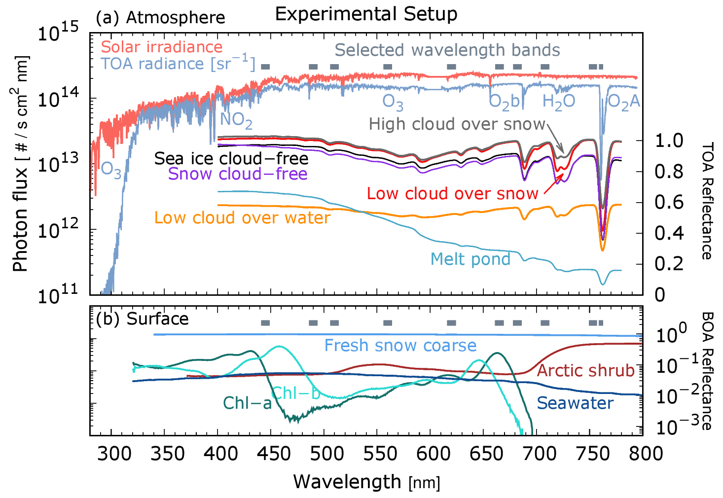
Figure 1Plots of the solar irradiance, the radiance of a cloud (Earthshine), and reflectances at the top (TOA) and bottom (BOA) of the atmosphere as a function of wavelength from 280 to 800 nm. The cloud radiance was observed by GOME on 15 May 2001, over the Kara Sea (80.53∘ N, 75.99∘ E). Modeled (nadir, solar zenith 40∘) displays a water cloud, placed at 3 km and optically dense 30, above seawater and snow, with cloud-free sea ice, snow, and melt pond spectrum. The lower panel shows the black-sky hemispherical reflectance at the ground of relevant Arctic surface components. Chlorophyll absorption is taken from Clementson and Wojtasiewicz (2019) and plotted for a May 2016 concentration of 12 mg m−3 observed in the Bering Sea (Frey et al., 2018). Arctic shrub and coarse snow data are taken from the ECOSTRESS and ASTER spectral libraries (Meerdink et al., 2019; Baldridge et al., 2009). Melt pond and sea ice albedos are from Istomina et al. (2013).
2.1 Reflectance data at TOA
To detect changes on daily, monthly, seasonal, and decadal scales, several measurements per day at an adequate spatial resolution must be made over several decades. The polar-orbiting spectrometer suite comprising GOME, SCIAMACHY, and GOME-2 (Table C1 for their specifications) makes measurements of at the same solar zenith angle and at several times per day as a result of the instruments' swath widths. They are a suitable choice, given the length and coverage of their records and their high spectral resolution, for the creation of the time series. Description of GOME can be found in Burrows et al. (1999), while SCIAMACHY and GOME-2 are, respectively, described in Burrows et al. (1995) and Munro et al. (2016). The detailed steps to harmonize measured by sensors of different technical specifications are given in Appendix C.

Figure 2Annual cycle of spectral RTOA at three wavelengths (λ = 510, 560, 760 nm) for the full record from 1996 to 2018. All sets exhibit the demarcation between months of steep (April–May–June) and flat (July–August–September) gradient of RTOA. This shift leads by 1 month melt onset (6 June), followed by sea ice opening, breakup, minimum (16 July–September inclusive), and freeze onset (4 October) as observed with satellite brightness temperatures (Smith et al., 2020). In the rightmost panel is the terminator location of the three sensors with the 85∘ N (grey line) common threshold used for monthly RTOA aggregation.
While the measurement of solar radiation scattered back to the TOA by GOME, SCIAMACHY, or GOME-2 takes place only during daylight, radiation in the thermal infrared (λ ≳ 4 µm), required to record the thermal emission from the surface and the atmosphere, is not measured by these sensors. Because of the different sensors' swath widths, the measurements in the solar spectral range have a northern latitude boundary (or terminator). This boundary is illustrated by plotting the pan-Arctic annual cycle of in Fig. 2. At the three wavelengths 510, 560, and 760 nm, the seasonality shows that summer months have lower and is higher otherwise. This darkening of the Arctic can also be seen by comparing the years at the beginning of the recording from 1996 with the most recent ones. However, this behavior occurs only between April and September. These are the months when the individual terminator of the three sensors reaches the latitude 85∘ N, this being the spatial threshold of common spatial coverage we set in the monthly average. As shown in Fig. 2, the other months (October to March inclusive) show that recent years are brighter (higher ) than those at the beginning of the time series. This is because the individual terminators move further south (Fig. 2c) and the coverage is considered insufficient for this to be studied further.
From Fig. 2 we identify two distinct behaviors of . The first is a period of steepest decrease, from April to June, and the second is a plateau of relatively flat , between July and September. The changes in surface reflectance between April and May are attributed to snow cover changes and those in June to sea ice changes (Smith et al., 2020). Over water, the timing of such transitions increasingly approaches the summer solstice, which is the day of strongest solar insolation, while it moves further away from it over land (Letterly et al., 2018). It is therefore reasonable to regard this day as a demarcation point between Arctic spring and summer.
In summary, we group April–May–June (AMJ) as Arctic spring and July–August–September (JAS) as Arctic summer. This distinction is explained by the sensors' measurement strategies and by the time-dependent physical processes leading to the transition from high to low Arctic reflectance in June to the minimum sea ice extent in September. We note that the definition of seasons is arbitrary and is determined by the breakpoints of the variable under consideration. In general, seasons can be astronomical, meteorological, or climatological. Ignoring the astronomical definition, the meteorological seasons are not suitable for our purposes because in May and June (respectively, the last month of meteorological spring and the first of summer) multiple scattering between the surface and the atmosphere still prevails, thus coupling both radiatively. The definition of ad hoc Arctic seasons ensures that the computed trends describe only those changes of caused by distinct underlying processes, which in turn determine the breakpoints in the time series of shown in Fig. 2.
2.2 Cloud products
In our study, the data are complemented by a record of cloud properties and broadband fluxes at TOA and the surface (see Sect. 2.3). These are inferred from the afternoon orbit (PM) of AVHRR sensors on board the POES missions. Despite the availability of the morning orbit (AM) AVHRR series, we found that only the AVHRR PM series fulfilled the calibration stability requirements which allow trend assessment to be made. Inspection of the time series of cloud properties and fluxes for the AM series shows that the drifts in local overpass time of the NOAA-12 platform before 2003 led to calibration offsets and that the scan motor errors of the NOAA-15 platform led to data gaps (Cloud_CCI Working Group, 2020).
One good reason for choosing this AVHRR record is the number of studies using these data in the Arctic. Our choice is driven by the maturity of the AVHRR data set of measurements; by its popularity; and by its successful use by the advanced, most recent, retrieval algorithm exploiting it. This AVHRR data set is in its third reprocessing, and the algorithm used to generate it has 15 years of development starting with ATSR-2 on board ERS-2. While improvements and validation have been documented in traceable documents (https://climate.esa.int/en/projects/cloud/key-documents/, last access: 23 February 2022), the cloud and flux records are presented by Stengel et al. (2020, and references therein). Recently, Vinjamuri et al. (2023) compared CFC, COT, LWP, and cloud top height (CTH) of this record with colocated measurements from four high-latitude stations across the Arctic and found no scale biases for the large majority of satellite-derived cloud products, except for the site located at Summit, Greenland (72.59∘ N, 38.42∘ W).
Some features that distinguish this data record from older AVHRR records are as follows: (1) the channels in the solar spectral range have been cross-calibrated with SCIAMACHY channels. SCIAMACHY is recognized for its accurate radiometric and spectral calibration. Because the part of our study dealing with is conceived in a way that the record is radiometrically coherent with SCIAMACHY (see Appendix C), this intra-band correction relates reflectance changes at visible wavelengths detected by SCIAMACHY to those by AVHRR, ingested in the cloud retrieval algorithm, which calculates τ and cloud albedo. (2) The cloud mask uses a neural network, trained on CALIOP data to take into account the extent of the underlying bright Arctic surface. (3) CTH has been calibrated using CALIOP profiles to account for the penetration depth of radiation inside a cloud. This is needed because the retrievals of CTH from all infrared thermal channels are influenced by this effect and yield a radiative cloud top height lower than the physical cloud top (Platnick, 2000; Rozanov and Kokhanovsky, 2005)
In this AVHRR satellite record, the cloud phase can be only liquid or ice. The input signal for AVHRR comes from the reflectances measured at 0.6, 0.8, and 3.7 µm. Given the different complex refractive indices of the water and ice phase across the SWIR wavelengths, the method is effective in separating the two phases. It is worth noting that Arctic cloud tops are predominantly in the liquid phase, whereas the mixed phase occurs in the middle of the clouds. This is the outcome of four airborne measurement campaigns, totaling 18 flights, reported in Mioche et al. (2017). Nonetheless, the mixed phase is not identified, despite its all-season occurrence (Morrison et al., 2012) and role in the Arctic climate (Tan and Storelvmo, 2019). This is because the data set is a neural network trained on the CALIOP cloud phase, which does not natively provide information on the mixed phase in clouds.
The application of the cloud algorithm to MODIS measurements, which take place in the same wavelengths as the AVHRR channels, has shown that the retrieval scheme is well aligned with the reference standards of CloudSat and CALIPSO data for CFC, CTH, τ, and the liquid thermodynamic phase. While agreeing on the sorting of cloud tops between water and ice phases, higher variability for IWP values lower than 50 g m−2 is found as compared to that in the reference DARDAR cloud data products (Delanoë and Hogan, 2010), but IWP histograms across the full range do not substantially differ (Stengel et al., 2015). Version 3 has improved version 2 in terms of precision, accuracy, and stability (Stengel et al., 2017). Even more relevant to our purpose is the scheme adopted to calculate broadband fluxes with the cloud properties described above.
2.3 Broadband flux products
The broadband fluxes in the solar and IR spectral regions are computed by solving the radiative transfer combining the two-stream approximation by Stephens et al. (2001) for the bulk bidirectional reflectance, transmission, and source terms within a plane-parallel atmospheric slab and the spectral band model by Fu and Liou (1992) for gaseous absorption. Six bands in the SW and 12 bands in the LW are calculated sequentially, ingesting local properties of clouds retrieved with a Bayesian technique (Sus et al., 2018; McGarragh et al., 2018), which provides estimates of the individual uncertainty at pixel level.
Specifically, effective radius and cloud optical thickness are the primary inputs for flux calculations together with solar zenith angle and ancillary data from MODIS climatologies of visible and near-infrared surface albedo, linearly interpolated to each spectral band center. Local vertical atmospheric profiles from ERA-Interim account for the p–T variations, while a constant aerosol optical depth of 0.05 and concentrations of well-mixed gases are assumed, the latter being linearly interpolated for their time-dependent increase. The combination of the above factors yields an accuracy of ± 3 W m−2 in outgoing LW radiation (OLR) when compared with observations by the broadband radiometer GERB on board the MSG-2 platform (Christensen et al., 2016). This value is in line with the radiometric accuracy of GERB, which is 1 % for clear-sky fluxes at TOA (Clerbaux et al., 2009) and with biases of 4–5 W m−2 against CERES observations, when a similar algorithm for the derivation of broadband fluxes is applied to CloudSat, CALIPSO, and MODIS measurements (Kay and L'Ecuyer, 2013). Specifically for the Arctic and for latitudes north of 66∘ N, winter OLR from AVHRR has been compared to the multi-model CMIP6 average (Linke et al., 2023). Based on their data we calculate an all-sky average bias of ± 3.59 W m−2.
The physical boundaries of clouds are additionally required to correctly compute scattering and absorption along the vertical. From the retrieved CTH and effective radius, the bottom cloud layer is calculated assuming a subadiabatic variation of cloud water path, separately for the liquid and ice phases. While this approach is appropriate for the shallow case (Merk et al., 2016), the thickness of deeper clouds is computed by combining a variable increase of water content matching within-cloud temperature profiles. The nominal accuracy limit, in this case, is reached at temperatures of less than 217 K (−56 ∘C), which exceeds the yearly climatological range for the Arctic (−25 ∘C February, +2.5 ∘C July; Hersbach et al., 2020), and AVHRR-derived cloud bottom height is found to be in good agreement within ± 369 m against ceilometer observations (Meerkötter and Zinner, 2007).
Radiative transfer is solved twice. First, all-sky fluxes are calculated with retrieved cloud properties and then the clear-sky fluxes, assuming that the pixel is devoid of clouds. This approach is in contrast to that employed with the MODIS cloud record and the CERES-EBAF radiation measurements at TOA, by which the interpolation of the measured clear-sky pixels serves as gap filling of all-sky pixels for the monthly aggregation of fluxes at BOA (Kato et al., 2013). AVHRR-derived fluxes at BOA have been validated by comparison with BSRN stations and the CERES-EBAF product (Stengel et al., 2020; Cloud_CCI Working Group, 2020).
Given the standard notation (all: all-sky, clr: clear-sky, +: upwelling, and −: downwelling fluxes), average comparisons with independent data show a good agreement for all downward fluxes and LW+. The average long-term relative bias of AVHRR-derived fluxes against CERES ranges from +2.9 % for SW to −2.7 % for LW. Validation with BSRN measurements in the period 2003–2016 shows that the bias (correlation) for SW is in the range [−6.16, +1.99] W m−2 () and [−3.02, +7.60] W m−2 () for LW. The average AVHRR-based estimates tend to be biased high at ≈ 20 W m−2 for SW+ < 100 W m−2, while the opposite holds for SW+ > 250 W m−2 with an average underestimation of up to −50 W m−2. In both ranges, the average relative bias amounts to ≈ 20 % (Stengel et al., 2020). This bias of higher spread can be due to the surface heterogeneity around the validation site, which influences the comparison of SW+ because of the difference in spatial scales between the satellite footprint and the BSRN effective point measurement.
The surface treatment in the satellite record is also a potential source of error because SW+ is equal to SW− times the surface albedo. While the actual sea ice extent is taken from measurements in the microwave (Henderson et al., 2013), a fixed value of spectral surface albedo is assumed throughout the record. The albedo of snow- and ice-covered surfaces is set to 0.958 at wavelength 630 nm, 0.868 (910 nm), 0.0364 (1.6 µm), and 0.0 (3.74 µm). The albedo is additionally area-weighted for fractional sea ice or snow cover scenes (Sus et al., 2018). Consequently, intra-annual variability and long-term changes in surface reflectivity are not accounted for. This would lead to an underestimate of actual surface albedos in those months having fresh snow and ice (spring) and overestimating during months of melting surface upper layers (summer). In the case of underestimation of surface albedo (or sea ice extent), we expect an overestimation of CRF and thus warming by the clouds and vice versa.
We do not expect differences in BOA fluxes as a function of solar zenith angles because the instantaneous fluxes are corrected for the diurnal cycle of solar illumination by adjusting the surface albedo and the atmospheric path lengths. The LW fluxes have been also corrected by using a cosine function derived from measurements of the geostationary SEVIRI sensor. The final aggregation is a good approximation to a true 24 h average (Stengel et al., 2020), needed to determine the true climatological mean of SW and LW fluxes and thus CRF. Consequently, also the seasonal averages (i.e., AMJ and JAS) are not expected to exhibit variations induced by solar zenith angle and directionality of surface reflection.
Misclassified cloudy scenes especially over dynamically bright surfaces (i.e., marginal and fractional sea ice zones) impact the calculation of broadband fluxes. This has been already noted in the first studies comparing ERBE and AVHRR cloud radiative forcing derived with different scene classification schemes (Li and Leighton, 1991). The conversion of directional radiance, measured at TOA, to irradiance requires the knowledge of the angular light redistribution function of the surface and atmospheric components. If this conversion is not accurately performed, the irradiance and SW above reflecting surfaces cannot optimally be calculated. Using the same data as that of our study, a low sensitivity of trends in cloud radiative forcing to the biases in cloud properties over surfaces of changing brightness has been found (Appendix D in Philipp et al., 2020, p. 7499).
Specifically, Philipp et al. (2020) assessed possible uncertainties in CRF trends by analyzing CFC biases as a function of sea ice concentrations (SICs) for the seasons defined in Sect. 2.1. For season AMJ, the bias is systematically flat from SIC 0 % to SIC 100 %. Given that our trend model is based on anomalies and not absolute values (see Appendix D), any additive component of the bias cancels out and the resulting trend is not affected by it. For season JAS, the bias is not flat and a multiplicative bias in CFC can propagate to CRF via SIC changes. However, the SIC bins of Philipp et al. (2020, Fig. A1) can also be regarded as the SIC variance over one location in time; therefore this effect is relevant only for those locations with a large dynamic in SIC (e.g., the marginal sea ice zone). If the SIC anomalies over one location in the marginal sea ice zone are not equally distributed about zero, irrespective of any trend, but progressively change over time, their distribution is not Gaussian but skewed. This leads to the addition of the time-dependent component in the CRF trend via CFC. Looking at Philipp et al. (2020, Fig. 8), the SIC anomalies for the marginal sea ice zone of the enlarged Chukchi Sea are normally distributed. Upon regression, any possible residual of a non-normal SIC distribution, reflected in CFC and propagating into CRF, would still be captured by the trend model (see Appendix D) which accounts for the length of the effective independent sample in the record.
3.1 TOA spectral reflectance
The time series, measured by GOME, SCIAMACHY, and GOME-2A over the Arctic region (60–85∘ N); anomalies; trends; and significance were harmonized (for more details see Appendix C and D). They are shown for wavelengths 510, 560, and 620 nm in Figs. 3 and 4. The values retrieved from the sensors MERIS (on Envisat) and GOME-2B (on MetOp-B) confirm that the correction scheme is successful for the spring (AMJ) and summer (JAS) months. The discrepancy between MERIS and SCIAMACHY in the fall and winter months, as long as sunlight is available, can be tracked to the different swath widths of the respective sensors. MERIS has a swath of 1150 km, whereas SCIAMACHY has a swath of 1000 km. This implies that with the onset of the polar night at high latitudes, the western part of the scan of both sensors (which are polar orbiters in descending node) will include increasingly dark Arctic areas, the MERIS scan being more northward leaning. Therefore, any averages of MERIS measurements will include more dark scenes than those in an average calculated from SCIAMACHY measurements. For this reason, the MERIS reflectances in the fall and winter months are generally lower than those by SCIAMACHY.
A consistent and consolidated data set results from the measurements of the three instruments. Seasonality is the dominant feature of Fig. 3. Maximum occurs in early AMJ when the polar day results in the Arctic being fully illuminated and the ice extent is close to its maximum. Analogously, minimum occurs from August to September when the days are shortening and sea ice coverage is at its minimum. The observed seasonal cycle of agrees with that calculated by models as do the observations of sea ice extent over the Arctic (Holland et al., 2008). This provides evidence to confirm that one dominant parameter in variability is surface reflectance (Sledd and L'Ecuyer, 2019).
Figure 3 shows that the standard deviation of for GOME is smaller than the other sensors. GOME has a considerably coarser pixel size than the follow-on sensors (see Table C1). This leads to different mean and standard deviations because the integration time of acquiring onboard electronics for a coarser pixel is longer than for a finer pixel. This averages out sub-pixel heterogeneity differently. We account for this effect by assessing trends not from mean values but from anomalies (see Appendix D) instead. The anomalies are customarily normalized with the standard deviation as a common technique for the analysis of records which might be heterogenous in scale, without changing the underlying sample distribution because standardization of anomalies is a linear transformation (Wilks, 2020).
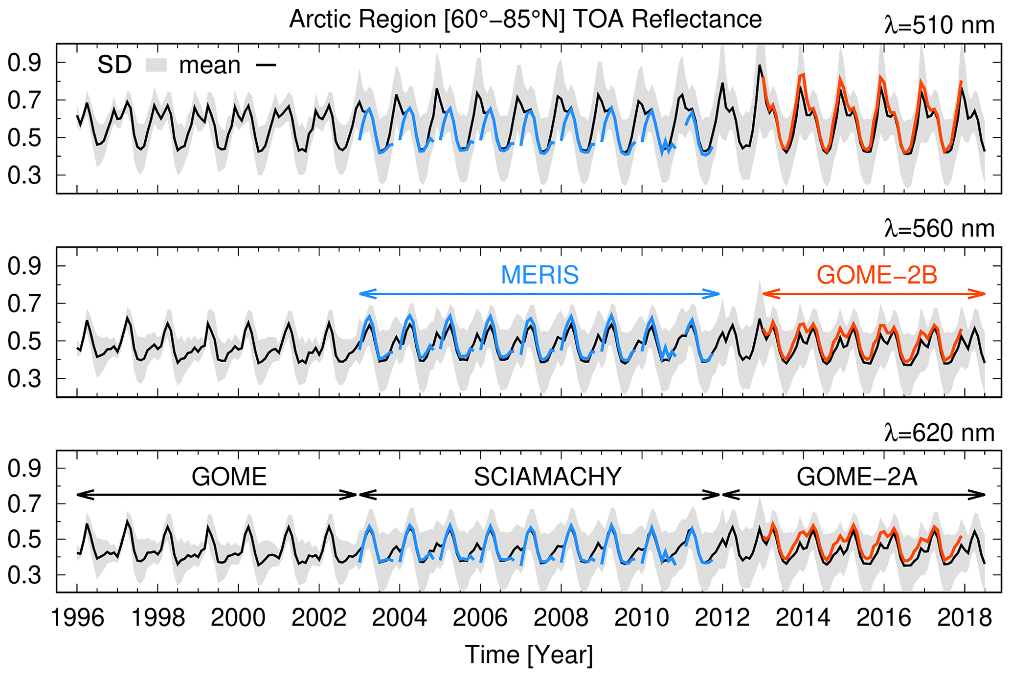
Figure 3Time series of mean absolute RTOA (red lines) and standard deviation (shaded grey) for the three wavelength bands 510, 560, and 620 nm derived from measurements of GOME, SCIAMACHY, and GOME-2A between 60–85∘ N. The companion sensors MERIS on board Envisat (blue) and GOME-2B on board MetOp-B (red) have been superimposed for comparison.
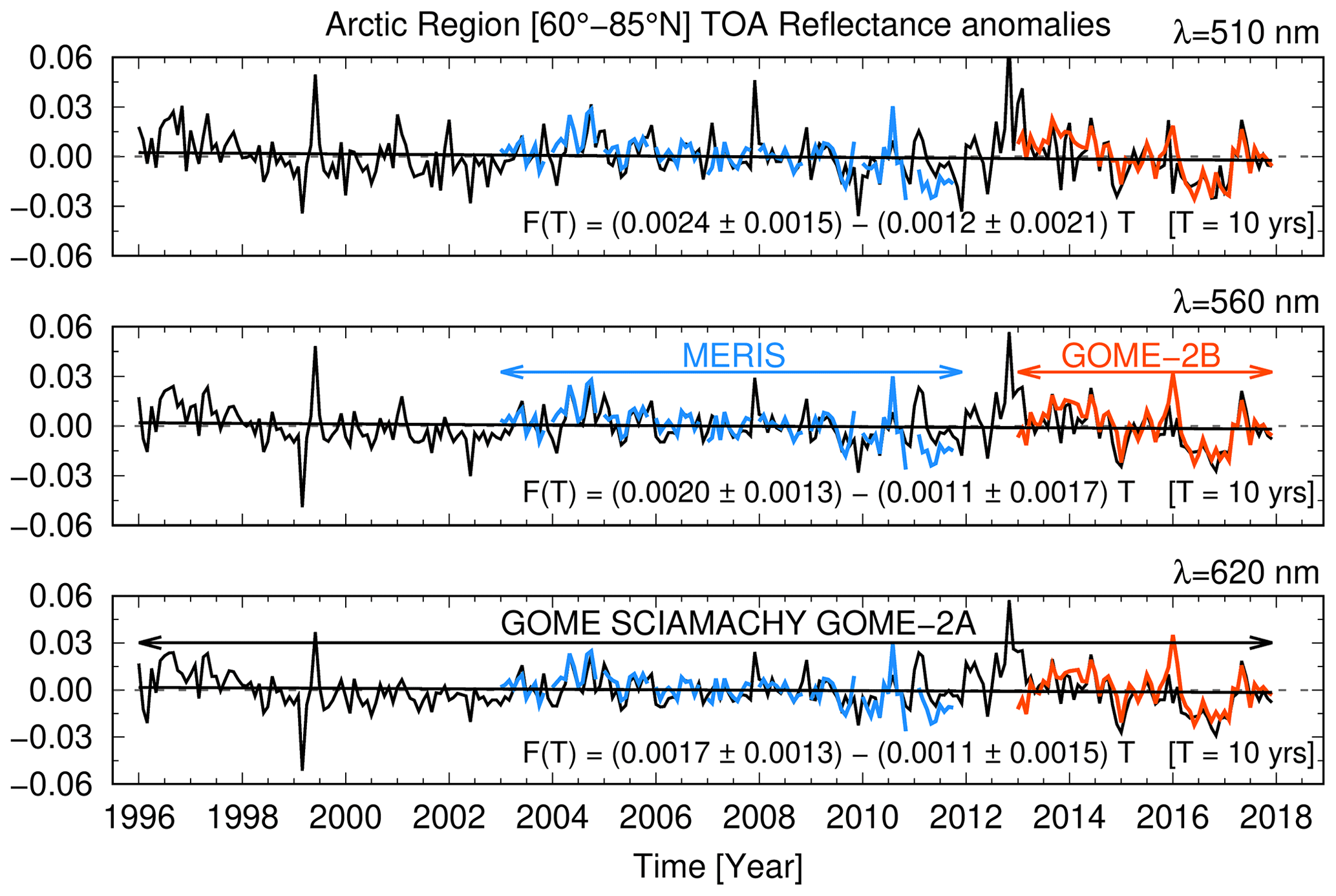
A negligibly small and statistically insignificant downward trend of for the three wavelengths in the solar range is seen in the anomalies of Fig. 4. The anomaly of is the difference between the value of and the climatological average value of at the given time of the year t (see Appendix D). In a warming Arctic, a substantial decrease in reflectance would have been expected due to sea ice loss.
In Pistone et al. (2014), a downward trend of all-sky albedo across the Arctic is reported. This is not compensated by an opposite trend in albedo as a result of increased cloudiness, which thus levels the recent pan-Arctic reflectance trend. However, their analysis is limited to oceanic regions (for open and ice-covered regions) and additional uncertainties are caused by the conversion from clear-sky to all-sky albedo at the beginning of their record. As the clear-sky signal is derived from the sea ice record with sensors for which the atmosphere is almost entirely transparent, the all-sky albedo is computed with a post hoc method adding the atmospheric part and is not the outcome of direct satellite measurements.
Moreover, Morrison et al. (2019) state that no significant relationship between CFC patterns and sea ice loss is observed during summer, but some are identified in fall months (Morrison et al., 2018). Such changes are not observable in the pan-Arctic RTOA anomalies. Rather, the reduction in reflectance is small and not attributable to a specific season. As a consequence, we need to ask whether the loss of reflectance associated with sea ice reduction is compensated by increasing CFC or brighter clouds, at the pan-Arctic and regional scale as well, and which processes lead to the small pan-Arctic RTOA trends.

Figure 5Sea ice concentration (SIC) for Arctic spring (a, b) and Arctic summer (c, d) for 1996 and 2017. Data from Walsh et al. (2019). The orange and red contours indicate SIC of 15 % and 75 %.
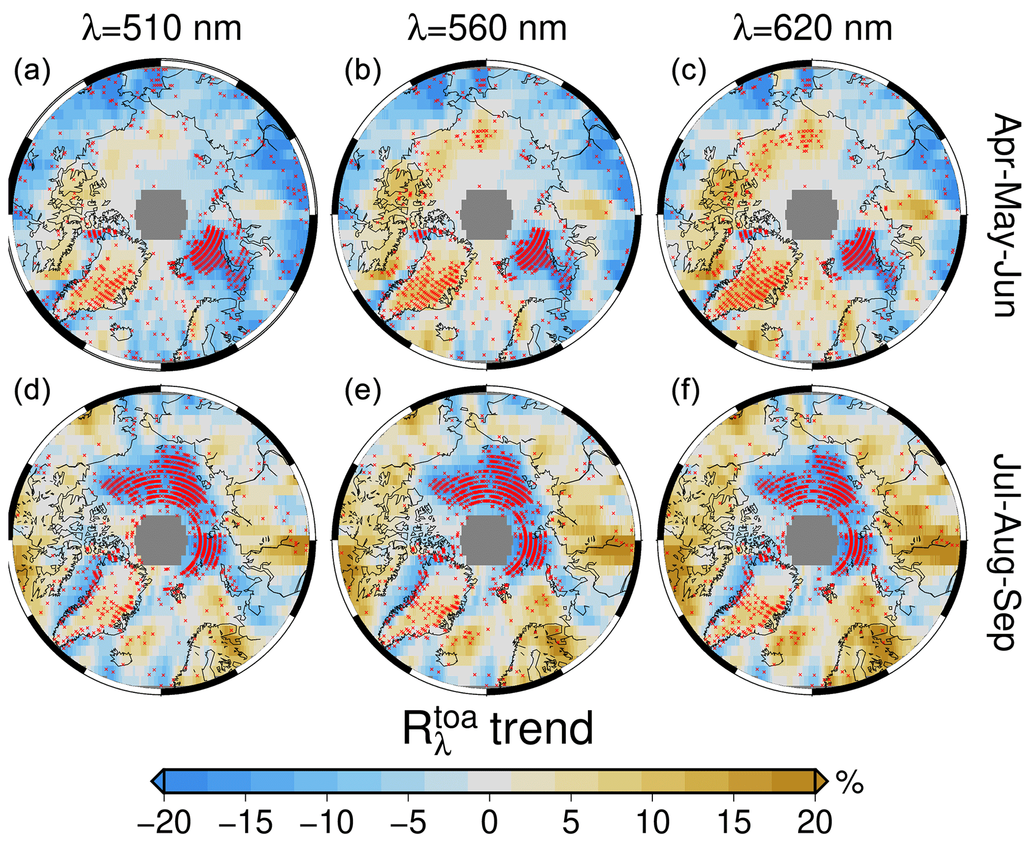
Figure 6Seasonal trends for 1996–2018 at selected λ for Arctic spring (AMJ, a–c) and summer (JAS, d–f). The values are relative to the leading season of the record. Stippling in red indicates significant trends at 95 % confidence.
To answer these questions in the following, we show the Arctic sea ice concentration (SIC) in 1996 and 2017 for AMJ and JAS in Fig. 5 and the trends for the wavelengths 510, 560, and 620 nm in Fig. 6. The mean seasonal sea ice extent (SIE) at 15 % and 75 % SIC is, respectively, coded in orange and red contours. While SIE is usually identified by a SIC threshold of 15 %, a value of 75 % better represents the geographical contours identified using . Moreover, Philipp et al. (2020) identify the 75 % SIE threshold as the demarcation between two distinct regimes of accuracy in broadband fluxes, which depends on the misclassification of satellite-derived CFC above bright surfaces.
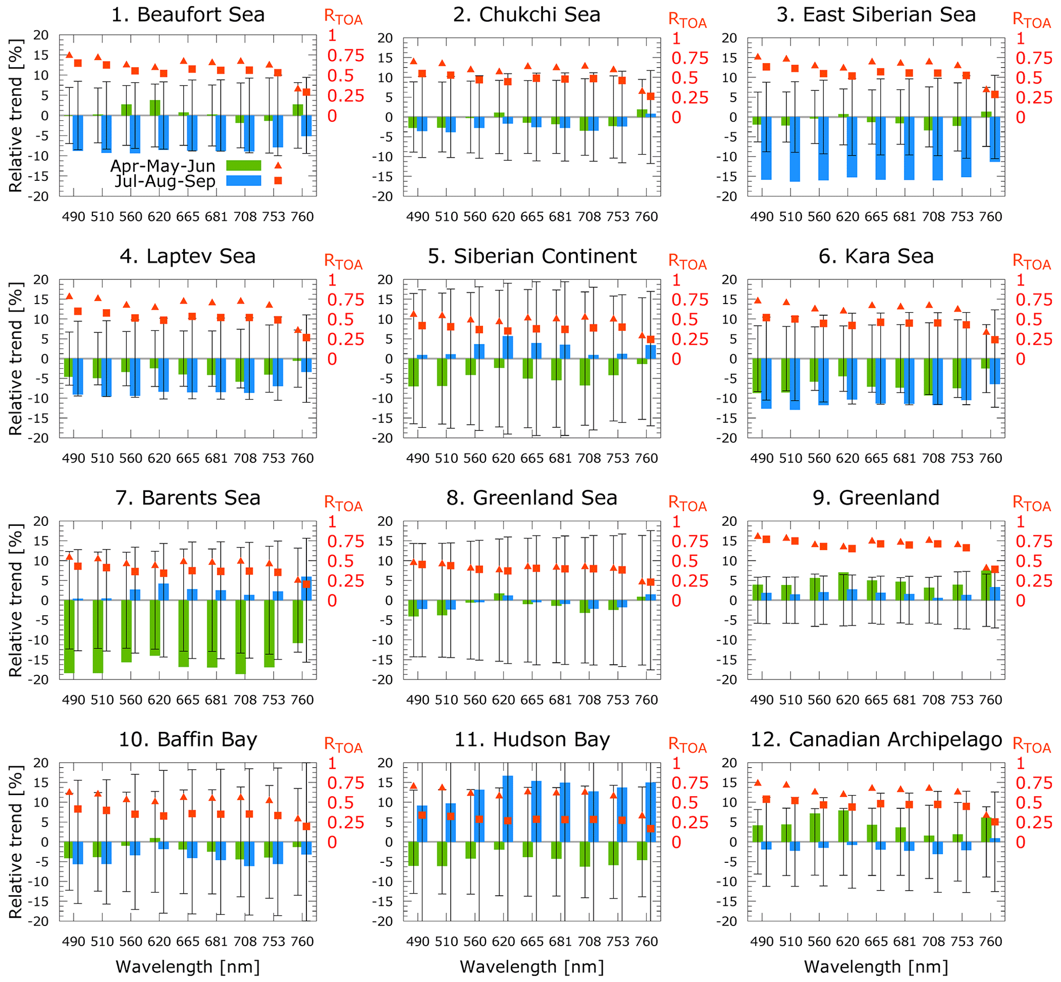
Figure 7 trends for the 12 regions defined in Fig. B1 for spring (AMJ, green bars) and summer (JAS, blue) months. The black bars represent the 2σ standard deviation of the trend. The secondary y axis displays the absolute mean values of reflectance for each Arctic sector. The trend values are relative to the respective lead season and express the total change throughout the record.
Similarly, Fig. 7 shows trends for the analyzed wavelengths for the 12 Arctic regions that are defined using the geographical subdivision proposed by Serreze and Barry (2014) and Wang and Key (2005a) (see Fig. B1). Trends for AMJ are shown in green, and the JAS trends for selected spectral bands are shown in blue. The red symbols show the absolute averages of the values at the beginning of the record for the respective seasons.
There are marked regional differences (Fig. 6). Those that are statistically significant (at 95 % confidence level) are shown with red crosses. For AMJ a significant negative trend over the Barents Sea is balanced by a positive trend at all three wavelength bands over Greenland, the Canadian Archipelago, and the western Arctic seas, such that the pan-Arctic trend remains almost unchanged. In JAS, the negative trend shifts towards areas of the Kara, Laptev, and Chukchi seas. These are Arctic areas having open oceans and are experiencing significant sea ice loss during the period of study (Fig. 5).
In general, the trends are negative and statistically significant in both seasons where sea ice retreats, such as in AMJ for the Barents Sea (Onarheim et al., 2018) and the perennial sea ice zone around the North Pole. For the remaining areas that cannot be directly explained by the difference in sea ice extent, we assume patchy residual sea ice concentrations below 50 % closer to Eurasia and the occurrence of melt ponds on the sea ice pack. In both cases, open ocean areas and freshwater lower the albedo of the scene sensed by the satellites, as can be seen comparing the 15 % and 75 % SIC contours in Fig. 5. The areas that do not show statistical significance are generally above the perennial sea ice during AMJ. These months are characterized by a small standard deviation and by a non-existent SIC trend (not shown).
The spectral dependence of the trends in Fig. 6 differs as a function of the sign. The negative trends are spectrally neutral in both magnitude and statistical significance. On the contrary, the areas of positive trends like the belt from the Canadian Archipelago and Beaufort and Chukchi seas in AMJ and, to a smaller extent, Greenland in both seasons show an increase in values and spatial statistical significance from 510 to 620 nm.
While we cannot completely rule out the broadband influence of ozone trends (see Appendix F) on reflectances, the spectral patterns are coherent with an increase in some cloud properties conducive to snowfall and a brighter surface. Despite its proximity to the Canadian Archipelago, Baffin Bay has changes in trends that would more closely match the eastern Arctic seas region. Over Hudson Bay, the trends show unusual patterns. They are largely positive in JAS and relatively strongly negative in AMJ.
Although not of the same magnitude, almost all regions show a reflectance change at 760 nm. This wavelength is the only channel with a very strong gaseous absorption and is not in the broadband continuum like all other channels. The 760 nm wavelength bears more information on light scattering aloft than at the surface because of the strong columnar absorption of atmospheric oxygen largely extinguishing photons before they impinge on the ground. Oxygen absorption is modulated primarily by CTH and, to a lesser extent, by CFC and optical properties such as cloud albedo (CA) and τ. In this context, where a positive trend value of at 760 nm is observed, greater than the other channels, we deduce a clear change in the occurrence of clouds or one of their physical or scattering properties. This is the case for Greenland during AMJ and JAS; for the Canadian Archipelago and the Barents, Chukchi, and East Siberian seas only in AMJ; and for the Barents Sea, Hudson Bay, the Atlantic corridor, and the Siberian continent only in JAS. Knowing that RTOA is influenced by scattering and absorption in the atmosphere (Sledd and L'Ecuyer, 2019; Donohoe and Battisti, 2011) and that the atmospheric RTOA can be additionally partitioned into the cloud, aerosol, and gas contributions, this prompted us to examine changes in those cloud properties which directly influence the spectral RTOA trends.
3.2 Cloud properties
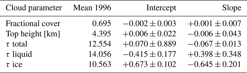
The globally validated and consolidated cloud record (Stengel et al., 2020) has first been analyzed across the Arctic (60–85∘ N). The top panel of Fig. 8 shows the time series of CFC and CTH. Both parameters show small, statistically insignificant, trends over the last 20 years. CFC has slightly increased by about 0.001 (+0.14 %) per decade, while cloud tops are lower by ≈ 6 m (−0.14 %) per decade. This finding excludes an explanation that reflectance loss at visible wavelengths, due to shrinking sea ice extent, is offset by more CFC or that the loss of CFC reveals more underlying bright surfaces. However, the bottom plot of Fig. 8 shows that the temporal trend over 2 decades for τ of liquid clouds has the opposite sign of that of ice clouds. τ of liquid clouds increases, statistically significantly, by about 0.4 (+2.85 %) per decade while the ice cloud τ decreases by 0.65 (−6.15 %) per decade in the same period. Altogether, the total τ of clouds has not changed, meaning that clouds have experienced a net shift from the ice to the liquid phase without changing their total opacity. The mean values for 1996 and trends of the above cloud properties are given in Table 1.
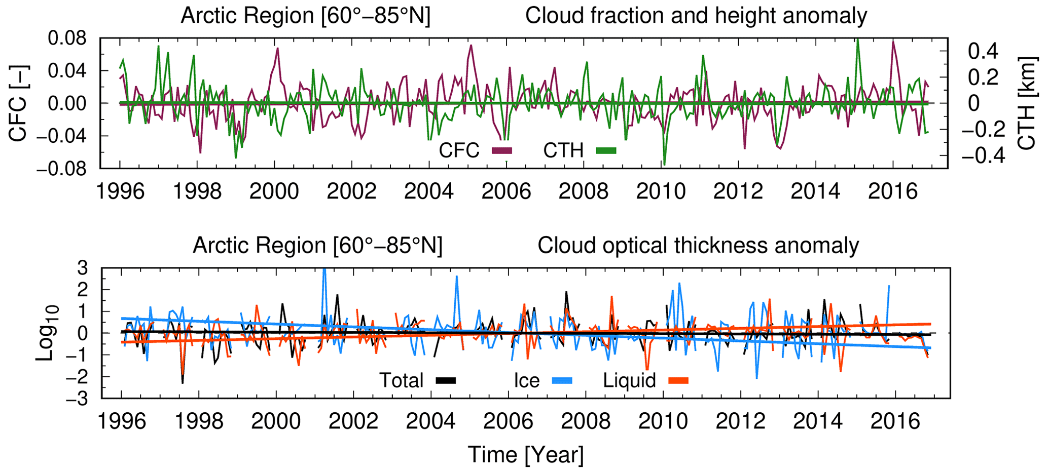
Figure 8Pan-Arctic anomalies and linear trends of cloud fractional cover (CFC), top height (CTH), and optical thickness (COT, τ) of all, liquid, and ice clouds.
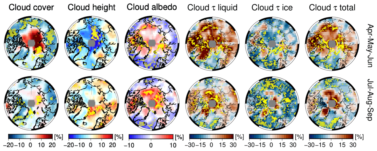
Figure 9For cloud cover (CFC), height (CTH), cloud albedo (CA) at 600 nm, and optical thickness (COT, τ) of all, liquid, and ice clouds, the panels show their seasonal breakdown. The trend values in percent (%) are relative to the property value at the start year (1996) in the record. Stippling in yellow indicates statistical significance at 95 % confidence.
Table 1Pan-Arctic mean values in 1996, trend intercept, slope, and bootstrapped 1σ (given for 10-year time interval) for cloud fractional cover, top height, and optical thickness τ of Fig. 8.
Similarly to the approach we used for the trends regionally and qualitatively, we map cloud parameters in the bottom panel of Fig. 9, adding also the albedo of clouds at λ = 600 nm. CFC trends are regionally partitioned and are seen to increase in the range of 5 %–20 %, where the greatest sea ice losses are observed. This occurs during AMJ and less extensively in JAS. Examples of this behavior are found in the Barents, the Kara, and the Laptev seas. On the contrary, large areas of a statistically significant decrease in the range of 2.5 %–10 % are homogeneously observed across land masses circling the inner polar belt. This includes Greenland and the Atlantic corridor, confirming past results (Hofer et al., 2017). More pronounced trends of the different cloud parameters, irrespective of their sign, occur in AMJ rather than in JAS. Hudson Bay is one of the few regions experiencing a seasonal trend reversal. The AMJ period is characterized by less cloudiness (−5 %), whereas the JAS period exhibits an increase of the order of almost 10 % over the last 2 decades. The resemblance to the trend reversal of all RTOA channels (Fig. 7) indicates that CFC changes primarily modulate over Hudson Bay. This is inferred from the absence of a change in trend sign for those cloud parameters that influence the reflectance in the solar spectrum, such as τ of liquid water and ice clouds in Fig. 9.
CTH decreases, especially where statistically significant trends are observed, during AMJ across almost all sectors of permanent and marginal sea ice (Beaufort, Chukchi, East Siberian, Laptev, and Kara seas) and over Baffin Bay. In the last 2 decades, CTH in these regions has decreased by 10 % on average. In JAS, however, CTH increases significantly from the Fram Strait, throughout the Barents and Laptev seas poleward, and in western Siberia. This is coupled with a slightly negative trend for Greenland and the surrounding waters, the southern Baffin Bay (the Davis Strait), the Beaufort Sea, and the East Siberian Sea.

Figure 10Trends (and 2σ standard deviation) of cloud fractional cover (CFC), top height (CTH), the optical thickness of liquid (COTL) and ice phase (COTI), albedo (CA), and liquid and ice water path (LWP and IWP) for the 12 sectors defined in Fig. B1 for spring (April–May–June, red bars) and summer (July–August–September, purple) months. The y axis displays the change relative to the leading season in 1996 and expresses the total change throughout the full record.
Total τ is split into liquid and solid cloud phases. The geographic distribution of the trends in Fig. 9 provides insight into which areas are responsible for the positive pan-Arctic trend in τ of liquid clouds (τ-liquid) and the negative trend for ice clouds (τ-ice). τ-liquid increases across the whole Arctic in AMJ except over the Atlantic sector and the southern part of Baffin Bay. The positive trend is maintained over northern Greenland and the Canadian Archipelago, around the North Pole, and on part of the Eurasian continent also during JAS. A positive trend of τ-liquid is correlated with a trend of opposite sign for τ-ice: this holds for all regions of permanent and marginal sea ice, the Canadian Archipelago, and Hudson Bay. Greenland, Baffin Bay, and the Atlantic sector show a different behavior: there is a 34 % increase in τ-liquid during AMJ and a 22 % increase in JAS. Notwithstanding the increase over certain areas (e.g., north Greenland), mean τ-ice over the Arctic regions remains nearly unchanged in different seasons. The liquid phase of clouds does not increase across the Fram Strait, whereas the ice phase decreases by roughly 20 % in both AMJ and JAS periods. Finally, the Atlantic sector (Greenland and the Norwegian seas) shows decreases in the τ for both the liquid and solid cloud phases during AMJ and JAS.
The polar plots of seasonal trends in cloud albedo (CA) in Fig. 9 show that the magnitude of the positive trends in JAS is larger than those of AMJ, but the spatial extent of the CA trend values are similar in both seasons. To a certain extent, the CA trends are geographically correlated with those of CFC and τ-liquid. Individual regions are grouped similarly to the RTOA polar plots: comparable distribution of CA are found over the most eastern and most western Arctic seas (Beaufort and Chukchi, East Siberian, Laptev, and Kara seas). Positive trends are almost invariably distributed over water masses, the Canadian Archipelago, and the northern part of Greenland, irrespective of the season. In contrast, clouds become less reflective at lower latitudes, southern Greenland, and the Atlantic sector. Over the Siberian land masses, this is not observed, and CA changes in the region are attributed to a competition between changes in CFC and τ-liquid. The loss of albedo due to cloud dissipation is compensated by the increment in albedo through increased τ-liquid.
Figure 10 shows the trends and the standard error (i.e., 2σ standard deviation) of five cloud properties (CFC, CTH, τ of liquid and ice phase, CA) together with the trend of liquid (LWP) and ice water path (IWP), from the same cloud record (Stengel et al., 2020). Changes in depend in the first place on changes in cloudiness and τ (irrespective of the phase), which in turn is a function of LWP, droplet or crystal effective radius (reff), and air density ρ (i.e., )). The sign of LWP and IWP trends confirms the τ trends. We infer that τ-liquid has increased as a result of the positive change of LWP.
3.3 Cloud radiative forcing
We compute the net radiative forcing derived only from clouds at the surface, or at the bottom of atmosphere (BOA), CRFBOA, from the differences between the downward and upward fluxes of SW and LW for all-sky and clear-sky conditions as follows:
The multi-year mean and trends of SWBOA, LWBOA, and total CRFBOA for AMJ and JAS are plotted in Fig. 11. The pan-Arctic and regional values are reported in Table 2 for AMJ and in Table 3 for JAS. Although not the focus of the current study because of the observational limitations of and the retrievals of optical cloud properties during the polar night, an annual perspective on mean CRF can be found in Fig. G1 and on CRF trends in Fig. G2, at both the surface and TOA.
The climatological annual pan-Arctic total CRF (see Fig. G1) is positive at the surface with the sole exception of the Greenland Sea. Minimum values are found over Baffin Bay and the Barents Sea. Over the Arctic Ocean, the total CRF is positive and amounts to ∼ 7.0 W m−2, which is lower than the 10 W m−2 reported by Kay and L'Ecuyer (2013, KE-13 hereafter), while over land masses clouds warm the surface by ∼ 11 W m−2. Our results are directly comparable to those of KE-13 because the algorithm computing the broadband fluxes is based on the same radiative transfer (Henderson et al., 2013), and the CRF is inferred from the difference between the all-sky and clear-sky atmospheric state, as in Eq. (2).
Among the differences that may explain the bias in CRF between our results and those in KE-13, we consider differences in spatial coverage of the Arctic and the spectral albedo of ice- and snow-covered surfaces. KE-13 defines the Arctic as the region between 70 and 82∘ N, while in this study the Arctic is defined between 60 and 85∘ N. The spectral surface albedo in this AVHRR record is 6 % higher for wavelengths in the visible and NIR (0.958 at 630 nm and 0.868 at 910 nm vs. 0.9/0.85 for the dry/melt months in KE-13), while it is lower for wavelengths in the SWIR (0.036 at 1.6 µm and 0.0 at 3.7 µm vs. 0.15/0.05 and 0.05/0.05 for the dry/melt months in KE-13). This means that the Arctic albedo in our record is indicative of dry and bright surfaces at shorter wavelengths but appropriate for melt and darker surfaces towards the infrared. This would lead to an overall underestimation of the (negative) CRF in the SW when compared to KE-13.
Having defined the Arctic as all those areas north of 60∘ N encompassing also low-latitude areas of the relatively dark surface, at a pan-Arctic scale clouds exert a negative SW radiative forcing in both AMJ and JAS, which is larger than the LW component by ∼ 12 and ∼ 18 W m−2 in the same seasons (Tables 2 and 3). However, the seasonal climatological mean CRF is highly variable across the Arctic and is regionally partitioned: clouds' total radiative forcing at the surface is positive over bright areas as a result of LW effects being larger than SW effects. For instance, this holds for the Beaufort, East Siberian, and Laptev seas and over Greenland, where total CRF becomes positive in both seasons and which corresponds to those Arctic areas over which the SW and LW CRF are also the smallest.
The combined effect of the brighter surface and comparatively low τ (irrespective of the phase) over Greenland (τ-liquid ∼ 8 in AMJ and ∼ 7 in JAS) increases SW reflectivity and damps upwelling LW. Minimum values in mean total CRF are seen over Baffin Bay, the Atlantic corridor, and the Barents Sea in both AMJ and JAS. For the same seasons, darker surfaces of the Atlantic corridor and Baffin Bay imply the presence of open water masses, which have higher temperatures and, therefore, emit LW more effectively. However, SW offsets LW and total CRF turns negative owing to larger average values of τ-liquid over the Greenland Sea (τ-liquid ∼ 15 in AMJ and ∼ 16 in JAS) or the Baffin Bay (∼ 15 in AMJ and ∼ 13 in JAS) (see Table G1).
At low surface albedos, typically less than 0.2, SW CRF outweighs LW CRF for the great majority of clouds, irrespective of their water content, τ-liquid, and sun illumination. Typical values of solar zenith > 65∘ correspond to latitudes north of 75∘ N, encompassing the Arctic Ocean in both AMJ and JAS. Resorting to Shupe and Intrieri (2004, Fig. 7), we obtain a lowest LWP threshold of ∼ 20 g m−2 at surface albedo 0.5 and ∼ 250 g m−2 at albedo 0.8. This means that, with increasing surface albedo, SW radiative effects may offset those by LW only at specific values of LWP and sun illumination angles, thus making CRF more sensitive to changes in cloud τ-liquid.
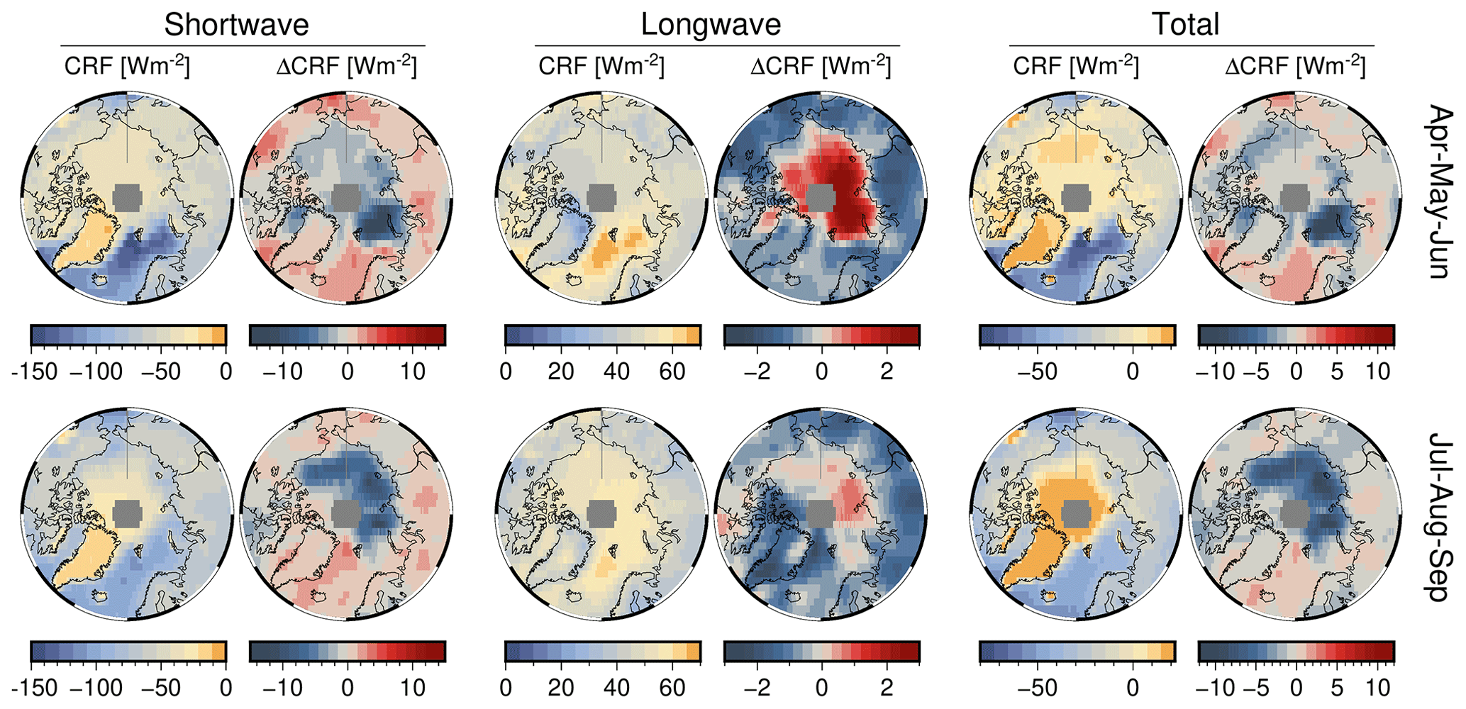
Figure 11For Arctic spring (AMJ, top) and summer (JAS, bottom), the multiyear mean cloud radiative forcing (CRF) and total change ΔCRF at the surface. None of the trends within the 2 decades of the record is statistically significant at 95 % confidence. The time of trend emergence (ToE) for each spectral interval is plotted in Fig. D1, and the first year of seasonal ToE is reported in Tables 2 and 3 for the 12 Arctic regions of this study.
Table 2For Arctic spring (AMJ), the pan-Arctic and regional climatological mean (1996–2016) of cloud radiative forcing (CRF in W m−2) at the surface (BOA, bottom of atmosphere) and total trend (W m−2 over 20 years) with 1 standard deviation. In parentheses, the time of emergence (in years) for the CRF trends to become statistically significant at 95 % confidence.

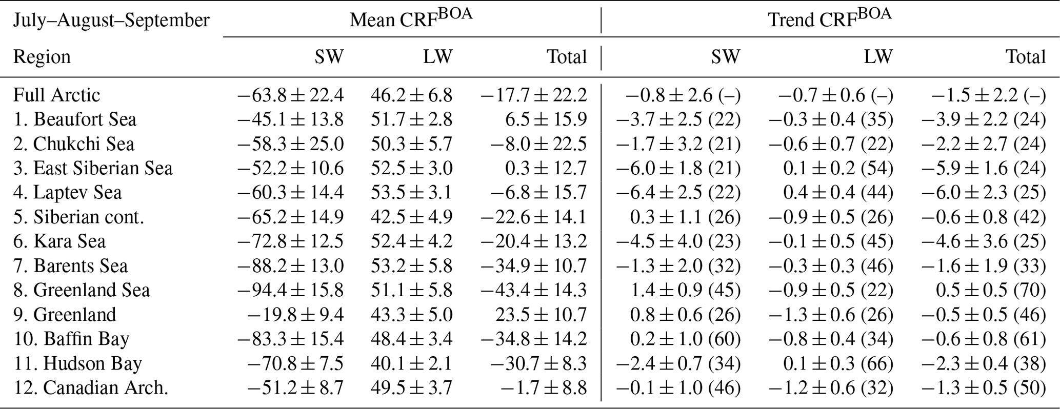
Consequently, the majority of clouds warm the Arctic surface, and our results are qualitatively consistent with current knowledge (Zygmuntowska et al., 2012; Kay and L'Ecuyer, 2013; Intrieri et al., 2002). The maximum cloud warming at the surface occurs over Greenland and to a lesser extent above sea-ice-covered regions in AMJ (East Siberian, Beaufort, and Laptev seas) and JAS (East Siberian and Beaufort seas). Otherwise, the other Arctic regions show a negative total CRF, from a minimum over the Greenland and Barents seas in AMJ to a less negative CRF over those regions influenced by the climate of the low latitudes (Baffin Bay, Greenland and Barents seas). Hudson Bay and the Kara Sea in JAS, respectively, show a total negative CRF of similar magnitude.
From the CRF trends of the last 2 decades (Fig. 11), clouds over the perennial sea ice zone increasingly cool TOA (see Fig. G2) and the surface (bottom of atmosphere, BOA) alike, while being neutral to positive over the Atlantic corridor and land masses at low latitudes. In AMJ months, maximal cooling trends at TOA (BOA) are for Kara and Laptev and extend along the Arctic Circle up to the northern section of the Baffin Bay through the Chukchi Sea, albeit dropping in magnitude to −0.9 (−0.8) W m−2 per decade. During AMJ, clouds have increasingly cooled the Siberian land masses and the marginal sea ice zones at an average rate, with the Barents Sea undergoing the strongest CRF drop by 2.5 W m−2 per decade.
Otherwise, the CRF trend at TOA and BOA during JAS varies from slightly positive over land masses, such as Eurasia, and over open waters in the Atlantic sector, the southernmost portion of Baffin Bay, and the Bering Strait. Cooling trends due to clouds are identified over Greenland for both seasons, having a rate of −0.5 W m−2 per decade. The influence of changes in surface albedo is manifested in these results. Where surface albedo remains almost constant (land masses, Greenland, and the Atlantic corridor) then CRF trends are of lesser magnitude. Instead, where the surface experiences more substantial changes, both seasonally and over the long term, trends in CRF are amplified, due to a greater influence of SW over LW.
None of the trends in CRF in Fig. 11 are statistically significant at 95 % confidence over the 20-year time frame of this data set. Thus, we estimate the time of emergence (ToE) in years for a trend to become statistically significant (see Appendix D, Fig. D1). The seasonal ToE and regional ToE are reported in Tables 2 and 3.
In the last 2 decades, the set of analyzed parameters provides a coherent geophysical picture: the Arctic has negligibly declined. This decline is less than that expected as a result of the loss of sea ice. We attribute the reason for the weak trend to a decrease in sea ice, compensated for by more liquid Arctic clouds and a concurrent simultaneous decreasing ice content in the clouds. Therefore, the thermodynamic phase separation of clouds manifests itself not only in the integral optical quantities (Figs. 8–9) but also in the water mass amount, considering Fig. 12.
To some extent, Wang and Key (2005b) anticipate the results of our work. The downward trend in the broadband albedo of −1.40 % per decade between 1982–1999 is confirmed by our weak all-sky trends, implying a sustained sea ice loss after 2000 and general darkening of the Arctic surface. However, the regional patterns in Wang and Key (2005b) match neither our results nor most recent knowledge (Hofer et al., 2017). The annual increase of 0.6 % in CFC over the Canadian Archipelago, Chukchi Sea, and Siberia and, in JAS, over Greenland reported in Wang and Key (2005b) is probably explained by the limited length of the analyzed record. For instance, CFC trends over Greenland level out before 1995 but turn strongly negative afterward, contributing to a significant loss of the ice shield mass (Hofer et al., 2017). This might explain the non-existent clouds' τ trends in Wang and Key (2005b), which is in contrast to the significant moistening across most of the Arctic of Figs. 8, 9 and 10.
4.1 Cloud-phase considerations
The cloud water path (CWP) is defined as the weighted sum of the two phases, whose relative occurrence is 0.54/0.46 % in AMJ and 0.63/0.37 % in JAS for the liquid/ice clouds, respectively. The seasonal correlation between CWP and its liquid/ice component is, respectively, 0.79/0.75 in AMJ and 0.57/0.84 in JAS, showing that the loss in ice water content is the main driver for the loss of total water condensate in clouds, more in summer than in spring. While highly variable at the pan-Arctic scale, the total change in CWP amounts to −0.51 ± 11.01 % in AMJ and −3.66 ± 7.29 % in JAS.
Notably, the majority of water path changes exceeding natural variability are those of LWP or IWP decrease over areas of sea ice loss and only partly of LWP increase over land masses, the Canadian Archipelago, some spots of Greenland, and the Beaufort Sea in JAS. Additionally, from Fig. 12 it can be seen that only those CWP trends in both seasons are statistically significant where the LWP and IWP trends are statistically significant too. This holds for the Fram Strait, the northernmost area of the Canadian Archipelago, the Bering Strait, and the coastal area of the Siberian continent. Only in AMJ do more statistically significant patterns of CWP trend emerge, these comprising areas from the Laptev, from the Kara, and throughout the northernmost part of the Barents seas.
In light of the results presented so far regarding the optical thickness and separation of the two cloud phases, it is reasonable to assume that this trend will continue in the future, allowing more patterns of statistical significance to emerge even where they have not been detected with 20 years of data.
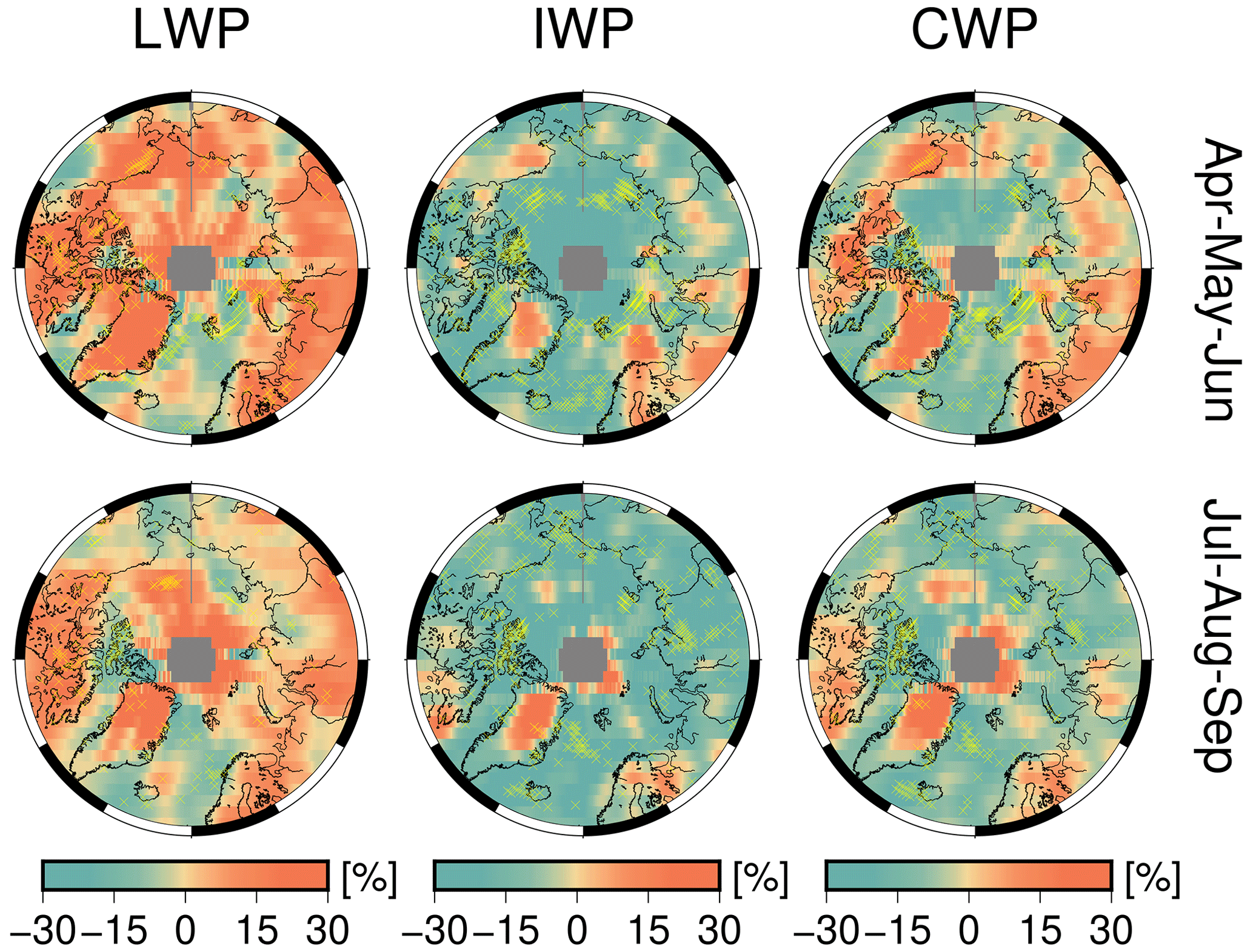
Figure 12Seasonal total trend, from the first season in the record, of liquid, ice, and total cloud water path (CWP). Stippling in yellow indicates areas of statistical significance at 95 %.
Atmospheric moisture fluxes are increasing as a result of more open waters and transport (Boisvert and Stroeve, 2015; Rinke et al., 2019). Marked regionality and seasonality of , cloud properties, and CRF across the Arctic are identified in four macro-regions, consistently exhibiting similar behavior: Greenland, the permanent and marginal sea ice areas, the Atlantic sector, and the land masses at lower latitudes.
Greenland has a unique behavior: trends at all wavelengths are positive, irrespective of the season (Fig. 7). The AMJ trends, up to 5 %, are even larger than those for JAS. This result is particularly surprising, given the insignificant CFC trend at the pan-Arctic scale and the local negative CFC trend in both seasons (Figs. 9, 10). Thus, these factors do not contribute to an increase in the overall reflectance. Therefore, we conclude that the increase in is due to the enhanced exposure of reflective surface in the southern part of Greenland, while a similar increase in the northern part is due to the simultaneous increase of τ-total (Fig. 9) and CWP (Fig. 12).
Similar behavior is found in Hudson Bay and the Canadian Archipelago, which show an increase in reflectance, in contrast to a general darkening of the Arctic. The mechanism by which these regions increase lies in the link between LWP and CA, through τ-liquid. In fact, τ-liquid changes sustain the correlated changes because of the non-linear relationship of CA to τ-liquid via LWP. It follows that a loss is overcompensated by more liquid clouds in the northern sector and by increased snowfall in the southern part of the Greenland continent. Cloud LWP has increased by 28 %–30 % over Greenland and by 14 %–16 % over Hudson Bay. The Canadian Archipelago also displays positive τ-liquid trends of 30 %, 14 %, and 22 %, respectively. Notably, the seasonal behavior of τ-liquid, increasing over Greenland, is not associated with CFC loss and a positive CRF change in the last 20 years. In contrast, cloud dissipation, increased by anticyclonic activity and concurrent temperature inversion strengths, is responsible for enhanced insolation at the ground and its concurrent melting effects (Hofer et al., 2017). In addition to cloud loss (Figs. 10 and 9 and Hofer et al., 2019), extensive ice melt in Greenland is also known to be enhanced by low-altitude liquid water clouds that have sufficient opacity to enhance downward LW flux but are also optically thin enough to allow a significant amount of SW flux to pass through. This results in the surface being warmed (Bennartz et al., 2013). Such clouds occur in the LWP region between 10 and 60 g m−2.
Figure 10 shows that the increase in τ-liquid of clouds and LWP over Greenland in spring and summer is among the largest in the entire Arctic (ΔLWP > 20 %–40 %). In both seasons, the cloud fraction decreases, and τ-liquid (as well as the LWP) increases spatially on average. Both effects impact upon the downward SW flux at BOA, but in the opposite direction, resulting in a small net positive change in SW CRF. For decreasing CFC over Greenland and in presence of an increase in near-surface temperatures, we expect a decreasing downward LW flux which might not be compensated by the LW enhancement by more liquid water in the clouds (Fig. 11, middle panel).
The changes in cloud properties and over Hudson Bay are exceptional. A 9 % increase in τ-liquid and minimal CRF changes are correlated to the greatest increase in the record in JAS. This area shows one of the largest CFC increases during summer months (Fig. 10), also corroborated by similar significant changes in AMJ and JAS observed in the reanalysis data (Fazel-Rastgar, 2020). The total CRF is −30.7 W m−2, while it is 2.7 W m−2 during AMJ. CRF trends point to a cloud cooling of Hudson Bay at a rate of −2.9 (AMJ) and −1.3 (JAS) W m−2 over the last 2 decades.
4.2 Dependencies of cloud radiative forcing
Cloud forcing at the surface depends on cloud property changes. The behavior is summarized in the seasonal and regional charts of Fig. 13, in which mean value and trend of SW, LW, and total CRF are shown as a function of τ-liquid of clouds, LWP, and CFC changes. The relationships between total CRF, τ, and LWP are more important in modulating radiation in JAS than in AMJ. This is the case when the underlying surface still has an albedo high enough to modulate CRF, as in the spring months over regions with sea ice. With a decreasing surface albedo, as in the summer months, SW CRF cooling dominates over LW CRF warming. As a consequence, Arctic regionality emerges from the clustering of the regions, especially in AMJ and to a lesser extent in JAS. We conclude that in the last 2 decades the net radiative effect of clouds on the surface is decreasing.
Those regions characterized by a darkening surface undergo a relative increase in SW reflection by more liquid clouds, leading to an increased cooling by clouds (ΔCRF < 0). This takes place over the Barents Sea, a region characterized by early sea ice loss in AMJ, and over the perennial sea ice zone (Beaufort, Laptev, and East Siberian seas), where a CRF decrease at a rate of −1 to 2 W m−2 is associated with greater cloudiness in AMJ and increasing τ-liquid in JAS.

Figure 13From left to right, regional and seasonal mean CRF, SW, LW, and total CRF trends at the surface as a function of τ trends for liquid clouds. The concurrent change in LWP is color coded while the increase (decrease) in cloudiness is given by a filled (outlined) circle.
From Fig. 13 we note that any positive τ-liquid trend corresponds to positive LWP changes for both seasons. Although not surprising, the AMJ changes in CRF do not correlate with either LWP or τ. In the JAS months, however, larger cloud optical densities and LWPs are matched by a decrease in CRF at the surface. This is the effect of darkening the surface that lowers the LWP value necessary for the CRFSW to dominate CRFLW. Excluding the Barents Sea, the variability of ΔCRF during AMJ is narrower (−4.2 to +0.9 W m−2) than during JAS (−6 to +0.4 W m−2). This is evidence of the importance of radiance from the underlying surface, which is larger in AMJ than in JAS. Overall, the radiative effect of CFC and τ is expected to be similar, provided that their changes in time agree in sign. Because CFC and τ change in opposite directions, the decreases in LW CRF and increases in SW CRF suggest a dominant influence of CFC rather than by water content in the clouds over Greenland. This CFC influence is still modulated, but not offset, by the changes in τ and CWP.
One exception is the East Siberian Sea in JAS where τ-liquid of clouds grows despite a lower content of liquid water. Notwithstanding the unexplained contribution of reff, we note that in JAS the East Siberian Sea has experienced a decrease in cloud altitude (see Fig. 10), which is a well-behaved parameter in the AVHRR record over most of the Arctic (Vinjamuri et al., 2023). Assuming that the cloud bases are unchanged, any change in CTH can influence the relationship through changes in ρ.
Figure 13 shows also that CFC changes (i.e., outlined vs. filled circles) modulate mainly the LW portion of cloud radiation in both seasons. The seasonal coefficients of determination r2 of SW CRF by CFC trends are comparable to those by τ-liquid trends. However, for the LW CRF, r2 by CFC is higher than that by τ-liquid (CFC: AMJ 0.98 for both above ocean and all areas; JAS 0.87 above the ocean and 0.94 above all areas. τ-liquid: AMJ 0.39/0.02 above ocean/all areas; JAS 0.65/0.19 above ocean/all areas). This is the case when clouds become optically denser and hence more reflective.
Quantitatively, with values of ΔCRFTotal= −1.4 W m−2 and ΔCF=3.03 %, we obtain the total long-term sensitivity −0.48 W m−2 %−1 over the Beaufort Sea in AMJ. The sensitivities of the SW and LW parts of CRF amount to −0.56 and +0.84 W m−2 %−1. Although averaged over one multi-year season only, our estimation is in line with measurements reported at the same location during the SHEBA campaign. The SHEBA sensitivity of W m−2 %−1 was seen to offset the SW for most of the year (with W m−2 %−1), thereby warming the surface, while cloud cooling took place only in midsummer months with the highest sun illumination and lowest surface albedo in late summer (Shupe and Intrieri, 2004).
Accordingly, we report a net total (SW + LW) sensitivity of −0.13 W m−2 %−1 in JAS, meaning that the SW cooling takes over LW warming during the Arctic JAS in the record. The warming effect from increased CFC in AMJ over these regions is directly linked not only to the retreat of sea ice, the onset of which is in late May (Smith et al., 2020), but also to the enhanced convergence of atmospheric water content originating from open Arctic oceans during years with anomalously low sea ice extent. Provided that the ocean cannot be an appreciable source of water vapor in the Arctic boundary layer, Kapsch et al. (2013) attribute an increased downwelling LW flux to the increased atmospheric opacity as a result of the convergence of moisture, in the form of clouds and/or water vapor (Rinke et al., 2019). Our results imply that this mechanism is evident in the year-to-year variability of exceptional sea ice lows and is also a long-term component at decadal timescales, during which atmosphere–ocean coupling effects are predominant.
4.3 Modeling considerations
From a modeling standpoint, we can validate past results (Morrison et al., 2019) for which the increases in cloud τ-liquid and LWP are projected to extend well beyond the middle of the present century. Constraining the cloud microphysics and thermodynamic phase will be crucial to project future Greenland melting (Hofer et al., 2019) and assess the sign and strengths of total cloud feedbacks (Gettelman and Sherwood, 2016; Ceppi et al., 2016). Given the actual and future Arctic temperatures, ice in the clouds will be increasingly depleted. Hence, τ-liquid and LWP will increasingly determine net cloud feedbacks (Bjordal et al., 2020).
When the cloud ice phase turns to liquid water, negative feedback is expected due to the offsetting of LW by SW. This is especially true in those months characterized by low surface albedo, under a stronger interaction with atmospheric radiation by liquid cloud droplets rather than ice crystals. For the rest of the year when the surface albedo is high and sun illumination is low or absent, the cloud feedback is expected to be more positive, which is a warming effect. If climate models do not correctly capture this behavior, i.e., they do not incorporate more supercooled liquid and mixed-phase clouds (Lohmann, 2002), unrealistically large amounts of ice result, effectively contributing to the uncertainty in determining the sign of the net cloud feedback.
We consider that this is one reason which may explain in part the discrepancy between the atmospheric components (CAM) of the Community Earth System Model (Gettelman et al., 2019, Fig. 2). While Huang et al. (2021) show that prescribing in the CESM1-CAM5 weaker scavenging of supercooled liquid droplets by ice crystals in spring months leads to an increase in available atmospheric liquid water and a concurrent increase in downwelling LW flux at the surface, we note that the CAM5 positive cloud feedback at Arctic latitudes becomes negative in CESM2-CAM6 as a result of improved modeling of the cloud phase. Coherently, CAM6 projects increased rainfall rates within a warmer Arctic in JAS at the expense of snow precipitation (McCrystall et al., 2021), as the outcome of poleward moisture streams and more liquid Arctic clouds.
Nevertheless, an improved representation of supercooled liquid clouds in CAM6 models (McIlhattan et al., 2020) does not necessarily result in better accuracy in describing cloud feedback. Although there is consensus that clouds, twice as bright in CAM6 than in CAM5, increasingly reduce the amount of SW energy accumulated at the surface through optical thickness and phase feedbacks (Goosse et al., 2018), thereby slowing the Arctic sea ice albedo feedback by 5 years over oceans and 2 years over land (Sledd and L’Ecuyer, 2021a), there are indications that clouds might accelerate the albedo feedback in some CMIP6 models (Sledd and L'Ecuyer, 2021b). This holds in summer months when the atmospheric contribution to Arctic TOA albedo, dominated by cloud reflectance, is higher than that of the surface. While suboptimal prescribed co-variability of clouds with the underlying sea ice is not ruled out, Sledd and L'Ecuyer (2021b) indicate that future efforts should focus on understanding the parameterization of the cloud microphysics, especially for those models that show a decrease in atmospheric reflectance.
4.4 Observational advances
Advances in observational techniques and process-level research are needed to assess unambiguously the relative roles of temperature and atmospheric particulate matter in determining cloud thermodynamic changes. In the absence of a systematic, pan-Arctic, aerosol indirect effect due to decreasing trends of ice-nucleating particles or cloud condensation nuclei (INPs or CCN), higher condensation rates (i.e., positive LWP trends) of small-sized cloud droplets can only nucleate and grow by a combination of changes in Arctic boundary layer depth within a saturated air volume. Different temperature regimes influence cloud albedo by changing the τ–reff–LWP relationship (Tselioudis et al., 1992) and favor droplet growth over condensation rates and vice versa (Lohmann et al., 2000).
To this end, the role of reff remains the unexplained factor in the relationship between τ and the water path. The reff size spectrum is modulated by the amount of water vapor and available particulate. While model and satellite data show a general moistening of the Arctic (Boisvert and Stroeve, 2015; Rinke et al., 2019), local on-ground (Graßl and Ritter, 2019; Schmale et al., 2022) evidence of a recent decrease in total aerosol burden is growing. However, INP or CCN cannot be directly inferred from changes in column-integrated extinction of total aerosol load, assuming a CCN decrease is in contradiction with the reff reduction via the Twomey effect. Alternatively, we speculate that the change in size spectrum or aerosol type might lead to optimal INP/CCN size and hygroscopicity (Heslin-Rees et al., 2020), although the total aerosol amount has decreased. This could be the case when anthropogenic aerosols decrease because of emission policy but natural aerosols increase due to more frequent boreal forest fires, increased sea spray, and marine biogenetic activity as a result of more open waters (Schmale et al., 2021).
Satellite-derived single reff values, such as those in the record analyzed in this work, are only representative of the droplet/crystal population at a level of ≈ 1τ from the cloud top (Platnick, 2000). We recommend that the available and relevant spectral observations are exploited (Kokhanovsky and Rozanov, 2012; King and Vaughan, 2012) to generate a pan-Arctic picture of in-cloud reff(z) profiles, which would optimally complement surveys based on spaceborne active techniques (Chan and Comiso, 2013; Matus and L'Ecuyer, 2017). reff(z) profiles, together with aerosol speciation at high latitudes (Schmale et al., 2021) and cloud bases (Lelli and Vountas, 2018), are essential in two ways. First, they constrain INP/CCN activation, supersaturation, and cloud particle number concentrations (Zheng et al., 2015; Grosvenor et al., 2018). Second, cloud fields will be more accurately separated according to their phase (liquid, ice, and mixed phase) and layering (low, mid, high level and multi-layered). We consider our results as upper bounds, and more vertical resolution will improve our understanding of the evolution of clouds in the Arctic.
Finally, a better estimation of the cloud-free surface albedo would enable us to pinpoint the broadband radiative interactions between the surface and the clouds. Recent results suggest that the SW effects of clouds at the surface almost double even in the presence of sea ice and snow. As a result, the total cloud radiative forcing shifts from warming to neutral values already at the beginning of the melt season in mid June (Stapf et al., 2020). This would imply that the results presented here underestimate the cooling effect of clouds.
This paper investigates clouds' roles in modulating Arctic radiation during sunlit months. We made use of 20 years of satellite data derived from a number of complementary sensors. The quantities investigated include spectral reflectance in the solar range. One of their advantages is that they are direct measurements and realizations of basic physical processes that do not depend on algorithmic assumptions. Two distinct changes in spectral reflectance were observed, which could be explained by sea ice retreat, particularly in Arctic spring, and changes in cloudiness during summer. This led us to analyze clouds' macro- and microphysical and optical properties, preparatory to understanding the radiative forcing of clouds at the surface.
Trend analysis of the above quantities composed a consistent picture: due to sea ice retreat, the loss in Arctic albedo at the top of the atmosphere was balanced by the increase in atmospheric reflectivity. This is explained by a statistically significant increase in the liquid phase of the clouds, balanced by a similar decrease in the ice phase. Since neither the total mass of condensed water in the clouds nor the cloud cover changed appreciably, it is inferred that the changes in Arctic atmospheric reflectance can be attributed to the increase in cloud reflectance due to the larger population of liquid droplets than ice crystals.
However, this behavior does not always apply to the entire Arctic but is regional and seasonal. The breakdown of the trends reveals common patterns. The perennial and marginal sea ice zones (from the Beaufort Sea until the Laptev Sea) have increasingly reflected less light in both Arctic spring and summer, while in summer months a generally greater decrease in spectral reflectance is observed. The Barents Sea exhibits statistically significant losses already in spring and a moderate increase of reflectance in summer, both indications of sea ice loss and subsequent change in cloud properties. Greenland showed a statistically significant increase in spectral reflectance, irrespective of the season, which could not only be explained by greater exposure of glaciated ground upon loss in cloud cover.
The resulting changes of total cloud radiative forcing at the surface indicate that over regions of marginal sea ice loss of transitional (high) albedo, the net effect is to increasingly cool the surface. This is the result of SW (cooling) effects offsetting LW (warming) effects in both seasons; this is less pronounced in Arctic spring than in summer. Locally, clouds have increasingly warmed the surface over the perennial sea ice pack, the North Atlantic, and the land masses at lower latitudes in both seasons, albeit at different rates, due to the relatively stable albedo of the surface. We have found a distinct relationship between trends in cloud radiative forcing and cloud properties. Cooling trends are attributed to the increase in cloud optical thickness, mostly driven by positive trends in liquid water path, over increasingly less reflective areas. At the same time, cloud cover changes seem to regulate mostly LW effects rather than SW effects.
In conclusion, while the climatological effect of Arctic clouds over sea ice is to warm the near-surface air and positively contribute to Arctic amplification, clouds also largely explain the trends in spectral reflectance through changes in their optical properties, which implies an increasing amount of supercooled cloud droplets. At the same time, the occurrence of cloud droplets at temperatures above the freezing point might also increase, especially over regions where sea ice has retreated. The higher reflectance of clouds results in a more negative radiative forcing at the surface, thereby locally dampening Arctic amplification, especially where sea ice retreats and most notably in summer. In this paper, we see a corresponding first signature of this tendency, which will become even more obvious and statistically significant in the future because the sea ice is expected to decrease even further in the years to come.
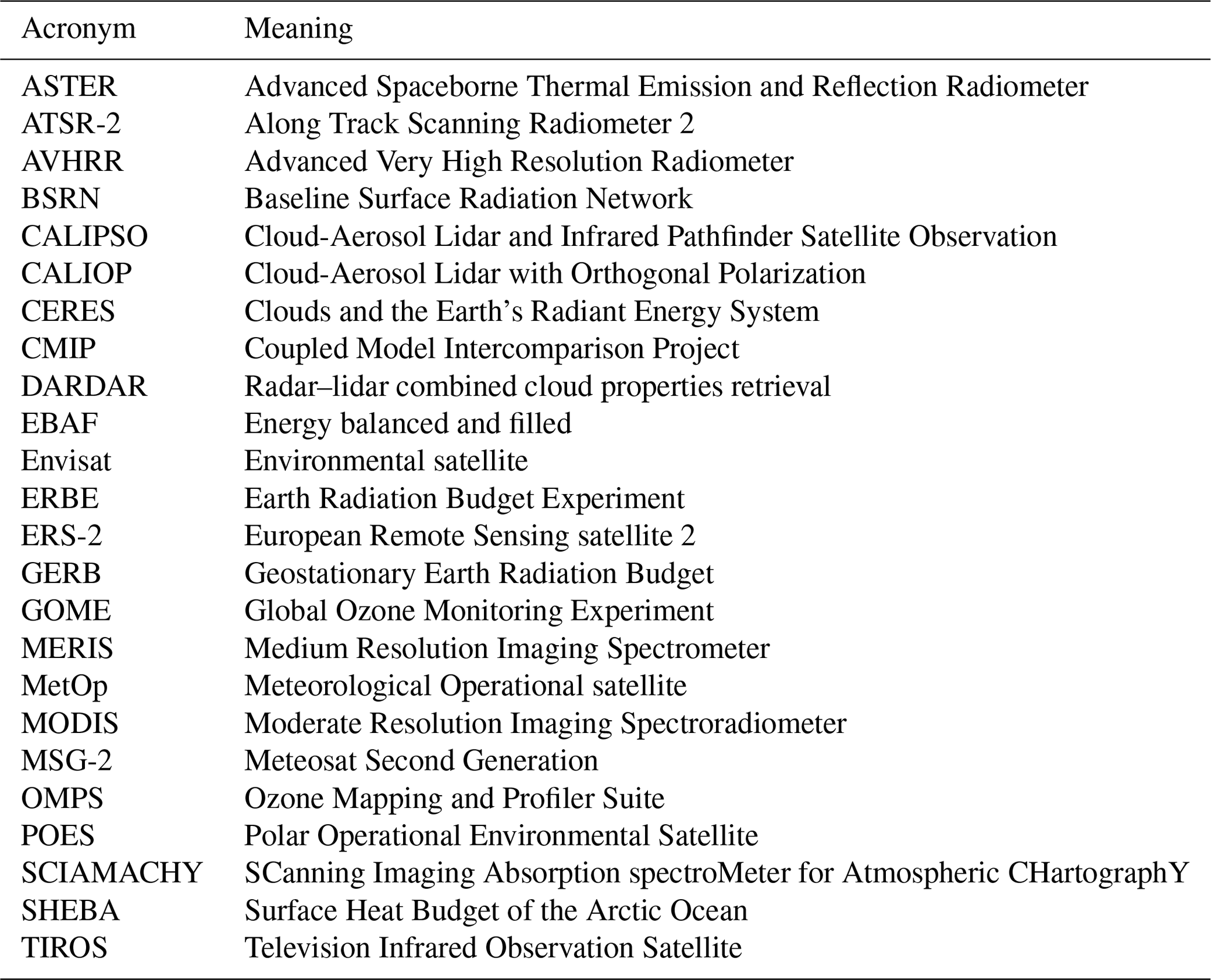
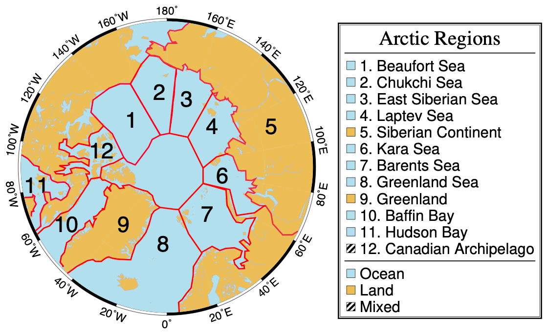
Figure B1Definition of the Arctic climate zones, identified by distinct geophysical settings, that will be used in this study to derive local trends of , cloud properties, and forcing. The geographical subdivision follows that of Serreze and Barry (2014) and Wang and Key (2005a).
Table C1 shows that overpass time, swath, and footprint size differ among the sensors used in this work. These sensors are payloads on satellites that fly in sun-synchronous orbits having different Equator crossing times. Errors in the in the Arctic arising from the 30 min time lag are considered negligible for averaged . Monthly aggregation leads to higher means for finer spatially resolved instruments than otherwise. Thus, intra-sensor radiometric harmonization is a prerequisite for the creation of calibrated time series and the detection of trends.
Different application-dependent approaches have already been employed. Krijger et al. (2007) derive gain correction factors based on the number of cloud-free scenes as a function of spatial resolution for maximization of usable trace-gas retrievals. Tilstra et al. (2012) separate the influence of scattering geometry and cloud occurrence to correct SCIAMACHY reflectances for the computation of the aerosol absorbing index at UV wavelengths. Both approaches are not suited to our goal. The former aims at the removal of the influence of clouds, which are a primary component of the Arctic environment. The latter examines instrumental performance in a spectral region that is not of direct interest as a result of potential radiometric degradation of sensors and of higher sensitivity to aerosols, whose radiative effects are comparatively small in the troposphere.
Conversely, Hilboll et al. (2013) elaborate a method to explicitly take into account the difference in the ground pixel size and spatial misalignment across sensors. This is achieved by projecting the orbit of one instrument onto that of a second instrument. In our case, we select SCIAMACHY as the reference sensor due to its well-calibrated spectral behavior and because it overlaps with both GOME and GOME-2A. A conservative area-weighted remapping scheme (Jones, 1999) is employed to derive the factor matrix transforming GOME-2A reflectances as they were measured by SCIAMACHY. Due to the frequent overlaps at high latitudes, only those GOME-2A orbits closest in time to SCIAMACHY are remapped. To extend the time series beyond the loss of Envisat on 8 April 2012, full SCIAMACHY geolocations, comprising 431 orbits per month, have been used as target tessellation for the rest of the GOME-2A record.
The downside of mimicking SCIAMACHY orbits, due to its design of alternating nadir and limb swath states, is the reduction of the GOME-2A sampling rate. This is compensated for in part by the inherently different cross-swath viewing geometries and changes in illumination. GOME projection onto SCIAMACHY has not been implemented. Not only do the two sensors overlap for a limited period of 6 months, but the relatively low sampling rate of GOME would have resulted in suboptimal statistics, even at a monthly scale. Validation has shown that GOME values are consistent with those of SCIAMACHY (see Fig. 3 in the main text). Remaining intra-sensor inconsistencies that cannot be compensated for, such as changes due to the dynamic radiometric response over dark-to-bright surfaces, will eventually be accounted for by the trend model.
Table C1Specifications of the instruments and data set versions selected for this work.

a Full coverage until May 2003. b Payload switched off since July 2011. c Lost contact on 8 April 2012. d Nominal end of GOME-2C record. e GOME-2A configuration change for tandem mode with GOME-2B on 15 July 2013. Foreseen extended lifetimes: November 2021 (GOME-2A), 2025 (GOME-2B), 2031 (GOME-2C).
We tested the assumption that bidirectional surface effects do not introduce error in the detection of the temporal trends of by inspecting monthly distributions of the scattering angle throughout the record, separately for each sensor. This is needed because is, by definition, a directional quantity and depends on the scattering geometry, that is on the phase function of different surface types and the thermodynamic cloud phase. Across the Arctic, the mean value of the scattering angle of 98.48∘ in 1996 shifts to 98.41∘ in 2018 for AMJ (−0.08 %) and from 97.03 to 96.55∘ for JAS (−0.51 %). These shifts are due to a change in the configuration of GOME-2A on 15 July 2013, allowing tandem operation with GOME-2B. The GOME-2A swath width of 1920 km has been reduced to 960 km, halving the across-track pixel size and, consequently, sampling differently the viewing zenith (Munro et al., 2016). However, these shifts are considered uncritical for this study and do not introduce artifacts in the record.
Trend detection is performed with the same technique for all the variables and parameters in this study. We illustrate the steps with reflectances. Dropping the subscript λ for readability, the values, measured by sensor i and aggregated at month t, Y(t,i), are modeled with
The μiC(t,i) denotes the intercept of the regression line, S(t,i) is the seasonal component of the time series, ωi is the desired trend value, and N(t,i) is the noise residuals embedded in the model after the regression is carried out. The term δ U(t,i) stands for the product of the level shift δ among the respective sensor records (Hilboll et al., 2013) with the step function U(t,i) needed to concatenate the individual time series at time Ti(t=0) (Lelli et al., 2014). The seasonality S(t,i) is accounted for by subtracting the average of each month from the respective monthly value. This method is similar to the harmonic expansion in the Fourier series, in which the coefficients are derived in the least squares sense. Both methods are equivalent and the choice of one method rather than the other does not introduce significant errors (Mieruch, 2009). The term δ U(t,i) is embedded by calculating the seasonality separately for each instrument. Its function is to correct possible artifacts due to the different overpass times of the respective spaceborne platforms.
While the offsets μiC(t), centered about their mean absolute value at the beginning of the time series, tend to zero upon the anomaly calculation, the last unexplored portion of the data is the noise component N(t,i), in which autocorrelative effects are buried. The time series are persistent in time and the autocorrelation for all Arctic regions after one lag. Thus, not all noise components of the record are random and they cannot be treated as Gaussian. This limits the informative value of any significance test and hinders the detection of trends.
Block bootstrap resampling (Efron and Tibshirani, 1993), belonging to the group of nonparametric methods, does not require prior knowledge of the analytical form of the underlying statistics of potentially non-normal data (Mudelsee, 2010). They rest on the block length of the effective independent random sample (Wilks, 1997, Eq. 19). An empirical sample distribution of the trend magnitude ω is then computed by scrambling n times the blocks of the original record. The resulting empirical distribution approximates the unknown ω probability density function. This allows finding the 2σω interval needed for a confidence level at 95 %. For all locations where the ratio , the trend magnitude ω exceeds natural variability and is termed statistically significant.

The CRF trends of Fig. 11 are not statistically significant within the 20 years of the record. Therefore, we estimate the time of trend emergence (ToE) by finding the time T (in years) needed for the measured trend to become twice as great as its standard deviation . The results are plotted in Fig. D1, and the first year of ToE is reported in Tables 2–3 for the 12 Arctic regions of Fig. B1. The is related to the standard deviation of the respective CRF time series σN, which can be regarded as the natural CRF variability, as follows (Weatherhead et al., 1998):
In Eq. (D2), we set dt=1 because ToE is expressed in years and the autocorrelation ϕ=0 because we have measured the trend from the independent sample of the record for which autocorrelative effects vanish already at the first lag of the monthly sampled original time series.
The cloud data set is generated using an optimal estimation framework, which allows the propagation of random and systematic uncertainties into the pixel-based retrievals. Following Eqs. (2)–(5) in Stengel et al. (2017), for each location i at time t, we calculate the true variability σtrue(i,t) and the uncertainty of the mean σ〈x〉(i,t) for the cloud property x from the mean of the squared pixel-based uncertainties 〈σ2(i,t)〉 and its standard deviation σSD(i,t).
Further, aggregation into monthly averages requires the uncertainty correlation c, or heterogeneity, relating σSD(i,t) to σtrue(i,t). Because c is not known beforehand, setting it to a fixed value is an arbitrary choice that does not account for the spatial and temporal relationship of algorithmic errors at the pixel level throughout wide-scale cloud fields. Hence, we exploit the fact that σSD→σtrue when c→1. This holds when the spatial sampling is the highest; thus we scale the number of successful retrievals of the cloud property x to c ∈ (0,1] and compute the c-dependent σtrue(i,t) and σ〈x〉(i,t).
Temporally, both σtrue and σ〈x〉 change as a function of c. Seasonal trends of c reveal an overall increase of a maximum of 3 % in AMJ and 1.9 % in JAS over the Barents Sea and throughout the East Siberian Sea, whereas c over Greenland, Hudson Bay, and the Canadian Archipelago exhibits a decrease of 0.6 % in both seasons. This translates into a change of ± 0.5 % and ± 0.4 % in σtrue and σ〈x〉, respectively. With this approach, the clouds' heterogeneity of the monthly averages is related to retrieval errors predominantly in the spatial but not in the temporal dimension. Limited to an observational analysis of the cloud record, while uncritical for trend assessments only, σ〈x〉 can be then successively used to label as meaningful those sensitivities of CRF to susceptible cloud property x, whose trend exceeds σ〈x〉.
RTOA trends at 560 and 620 nm capture the Chappuis ozone absorption band having a broadband maximum centered about 602 nm and two wings stretching between 525 and 675 nm (Gorshelev et al., 2014). Analyzing seasonal stratospheric and total column ozone, we can determine an effective modulation of RTOA trends by ozone. Ozone data in Fig. F1 are locally derived from GOME, SCIAMACHY, and GOME-2A for the total column values (Coldewey-Egbers et al., 2005) and with SCIAMACHY and the OMPS Limb Profiler measurements for the stratospheric column portion (Flittner et al., 2000; von Savigny et al., 2003; Arosio et al., 2019) in the time window 2003–2018. The tangent height of 41.3 km is selected due to its highest sensitivity to stratospheric ozone concentrations, which peaks at about that altitude.
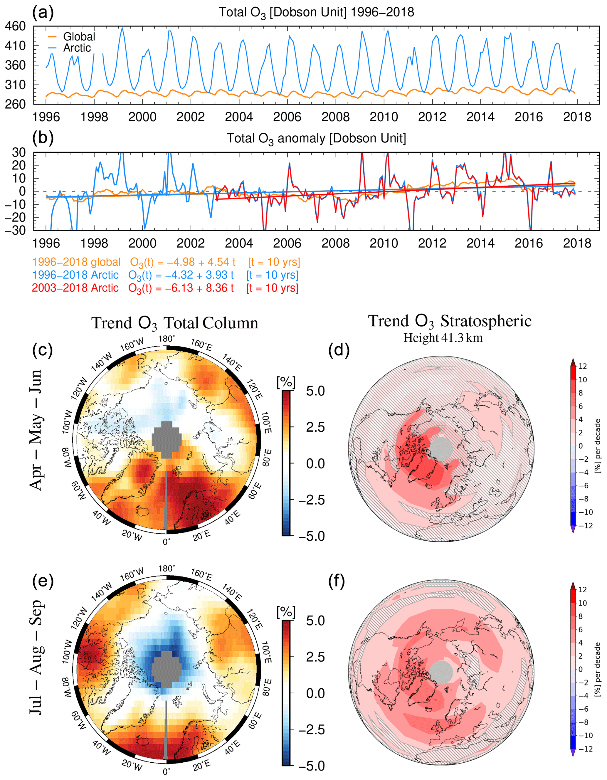
Figure F1(a, b) Global and Arctic record of total ozone with the respective anomalies and trends. The Arctic time series has been additionally shortened to match the length of the stratospheric ozone column. (c–f) Trends (% per decade) of total (c, e) and stratospheric (d, f) ozone between 2003 and 2018 are plotted for spring (AMJ) and summer (JAS) months.
Ozone is produced in the tropics, and circulation patterns transport it poleward. It is usually located above the tropopause, and its concentrations are higher during the winter months and lowest in the summer months. Despite its high variability through the year, total ozone trends are generally small in the order of ± 1 %. Focusing on the Arctic, the average total ozone is 353 DU and also exhibits a distinct maximum in spring months and a minimum in summer months. The Arctic-wide trend of total ozone is positive by 3.9 DU (+1.1 %) per decade, in line with global values.
Greater significant positive trends, ranging from +4 % to +10 % per decade, are found in stratospheric ozone. They are centered above Greenland and stretch out along the 75∘ N parallel from the Greenland Sea through the Beaufort Sea in spring (AMJ) with a long tongue over the Siberian continent in summer (JAS). Contrasting the total with the stratospheric column yields the influence of the tropospheric ozone only. For those locations where the trend in total ozone is absent but positive in the stratosphere, a negative tropospheric trend can be deduced. This mechanism is consistently found above 70∘ N from the Canadian Archipelago through to the East Siberian Sea, irrespective of the season, together with the sustained positive trend above the Atlantic (the Greenland Sea), the neighboring Barents Sea, and the northern part of mainland Greenland (Gaudel et al., 2020). This reverses in a dipole fashion in JAS, when patterns of positive trends in total ozone are advected southward. In summary, when analyzing trends at λ = 620 nm, and to a lesser extent 560 and 665 nm, changes in ozone contribute to those Arctic sectors affected by the meridional dynamics of air masses in which the stratospheric ozone is increasing. The most eastern Arctic sectors (East Siberian, Laptev, and Kara seas) have a smaller contribution from ozone changes than the western sectors. This is consistent with a neutral ozone trend observed over these areas.
Finally, we speculate that a surface warming of the Arctic might inflate the tropopause, inducing the production of polar stratospheric clouds as a result of colder temperatures. Lower ozone would absorb less UV and visible radiation, cooling the stratosphere further and potentially accelerating further its depletion. Albeit within natural variability, Turner et al. (2009) held stratospheric ozone depletion responsible for a change in the wind flows and patterns across the South Pole, stimulating anti-correlated changes in sea ice extent of the Antarctic continent. This hypothesis could also be tested for the Arctic, using the results from this investigation.
Table G1Multiyear seasonal means (± standard deviation) of cloud properties for the full Arctic and 12 regions of Fig. B1.
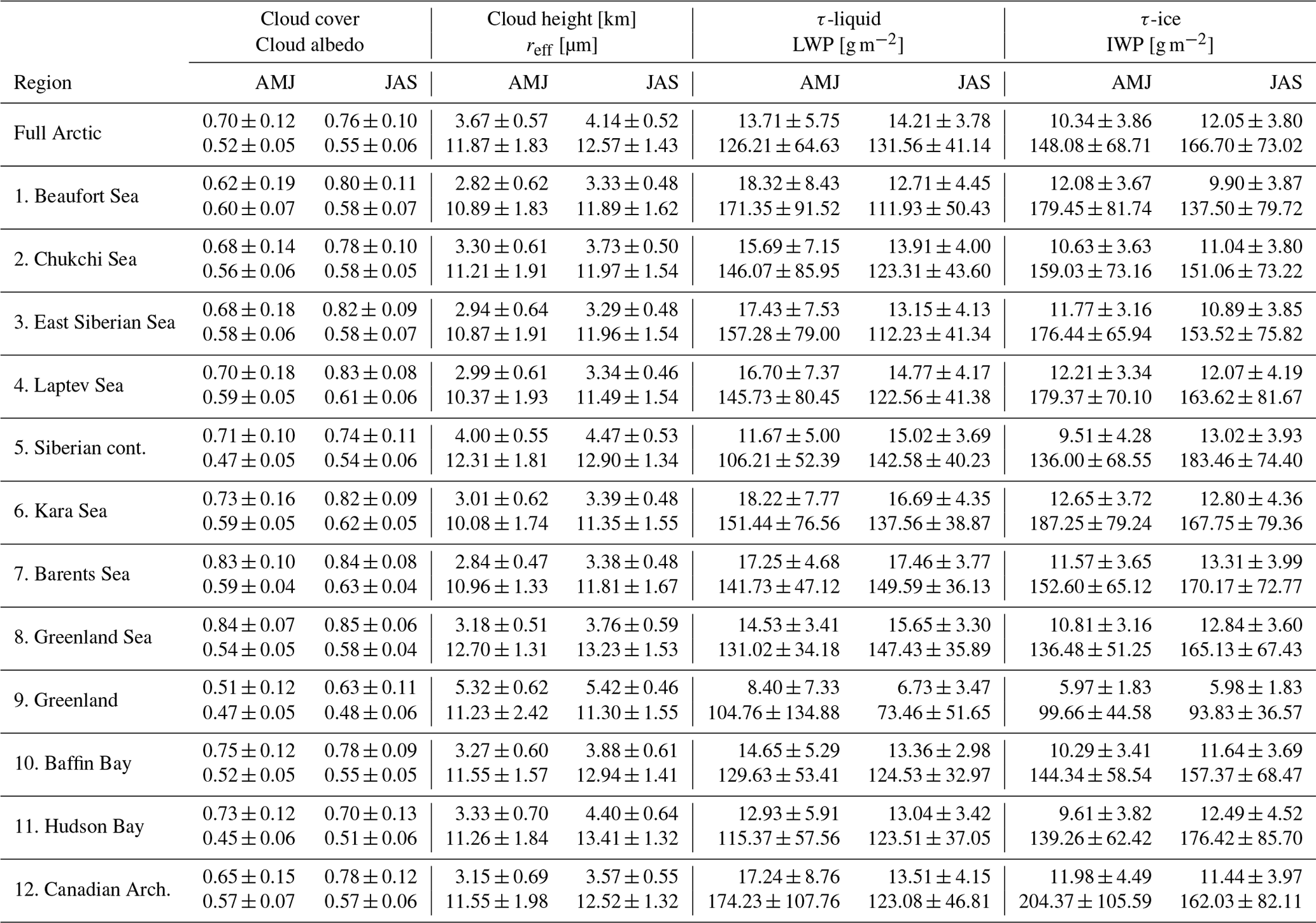
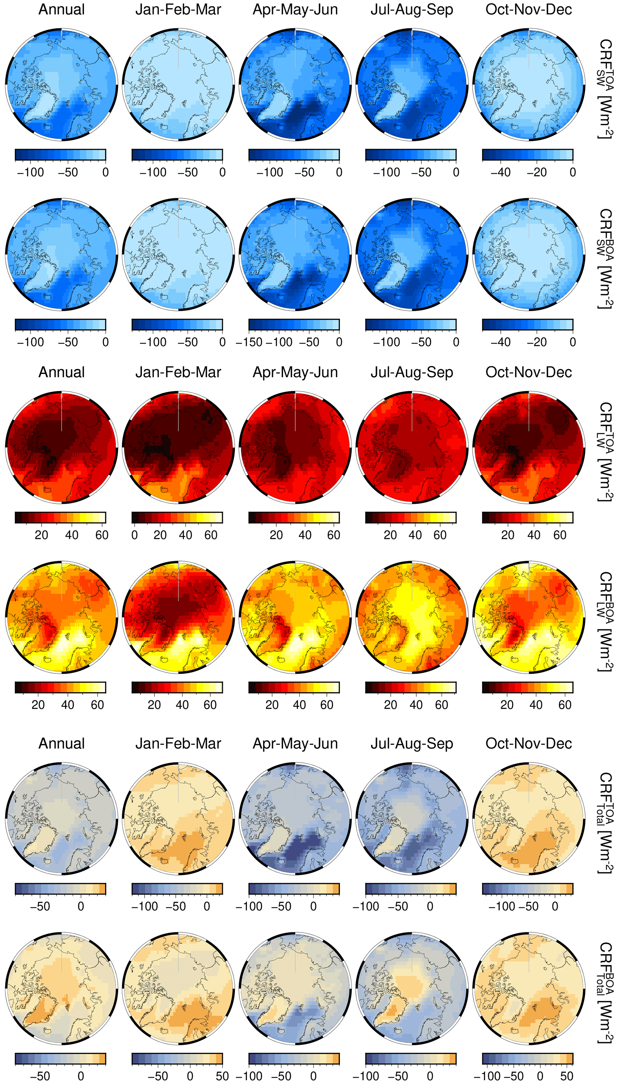
Figure G1From left to right, annual and seasonal average values of SW (rows 1–2), LW (3–4), and total (5–6) cloud radiative forcing (CRF, W m−2) at TOA and BOA, respectively. Note the different color scales to match the CRF ranges.
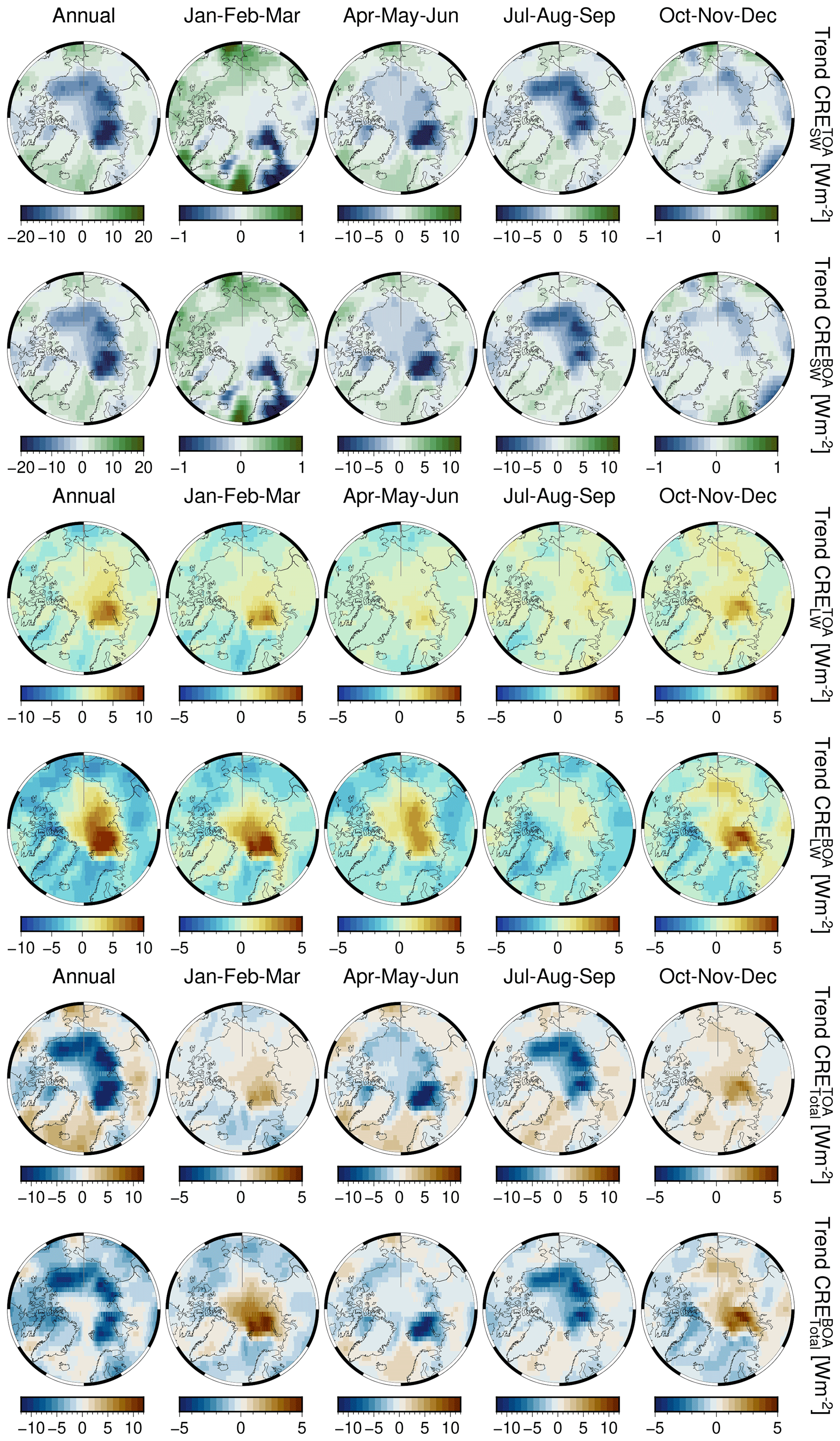
Figure G2From left to right, annual and seasonal trends of SW (rows 1–2), LW (3–4), and total (5–6) cloud radiative forcing (CRF, W m−2) at TOA and BOA.
Perl and Bash code to extract, harmonize, grid, and analyze all data records is available from the first author upon request. Essential software such as Generic Mapping Tools (GMT, https://www.generic-mapping-tools.org/, Wessel et al., 2019) and Climate Data Operators (CDO, https://code.mpimet.mpg.de/projects/cdo, Schulzweida, 2022) is available on the respective websites.
Native L1 orbital data (versioned with total size) of spectral reflectance are available at https://earth.esa.int/eogateway/catalog/, last access: 18 February 2023 for GOME (v5.1, 2.47 TB), SCIAMACHY (v9.01, 16.98 TB), and MERIS (v8, 23.75 TB in Reduced Resolution). GOME-2A and GOME-2B (v5.3 until June 2014, v6.x afterward, 58.28 TB each) have been accessed via EUMETCast. We recommend users download the newly reprocessed GOME-2 Fundamental Data Record (FDR) v3 available at http://doi.org/10.15770/EUM_SEC_CLM_0039, last access: 18 February 2023 (EUMETSAT, 2022). The Arctic spectral subset (10 wavelength bands north of the 60∘ latitude, ≈ 13 TB) of L1 orbital data is available upon request. Due to obvious size limitations, we have prepared a monthly spectral reflectance data set available at https://doi.org/10.1594/PANGAEA.933905 (Lelli et al., 2021). Cloud and flux data are available at the Deutscher Wetterdienst (DWD) website https://doi.org/10.5676/DWD/ESA_Cloud_cci/AVHRR-PM/V003, last access: 23 July 2022 (Stengel et al., 2019). Spectral albedo of sea ice and ponds is taken from Istomina et al. (2013).
LL, MV, and JPB conceived the research. LL led code development, processed orbital reflectance data, analyzed all records, and wrote the paper. NK and MV processed the orbital reflectance data and analyzed the record. Funding acquisition was done by LL, MV, and JPB. All authors contributed to the interpretation of the results and the final drafting of the paper.
The authors declare that they have no competing interests.
Publisher’s note: Copernicus Publications remains neutral with regard to jurisdictional claims in published maps and institutional affiliations.
We thank Kamesh Vinjamuri (IUP Bremen) for the validation of AVHRR radiance and cloud optical properties, Carlo Arosio (IUP Bremen) for provision of stratospheric ozone data, Alessandra Cacciari (EUMETSAT) for the interpretation of GOME-2A sensing geometry, and the ESA Cloud CCI working group for processing the AVHRR data set. For valuable discussions, we acknowledge Ann Fridlind (NASA/GISS), Tido Semmler, Felix Pithan (AWI Bremerhaven), and especially Kerstin Ebell (University of Cologne). Luca Lelli, as a visiting scientist within the NASA/Goddard Space Flight Center PACE (Plankton, Aerosol, Cloud, ocean Ecosystem) project, was supported by the Alexander von Humboldt Foundation. Zhanqing Li (UMD – University of Maryland), Jeremy Werdell (OEL – Ocean Ecology Laboratory, NASA/GSFC), and Andrew Mark Sayer (NASA/GSFC and USRA – Universities Space Research Association) have been instrumental in the establishment of this cooperation. Luca Lelli thanks Theofanis Stamoulis for the initial steps with reflectances, which eventually evolved in this paper. The time devoted by the two reviewers in scrutinizing our work and the competence of the editor in handling the review process are greatly appreciated.
This research has been supported by the Deutsche Forschungsgemeinschaft (grant no. 268020496) within the project “ArctiC Amplification: Climate Relevant Atmospheric and SurfaCe Processes, and Feedback Mechanisms (AC)3” as the Transregional Collaborative Research Center (TRR) 172 and the Alexander von Humboldt Stiftung (Feodor Lynen Research Fellowship 2020).
The article processing charges for this
open-access publication were covered by the University
of Bremen.
This paper was edited by Timothy Garrett and reviewed by two anonymous referees.
Arosio, C., Rozanov, A., Malinina, E., Weber, M., and Burrows, J. P.: Merging of ozone profiles from SCIAMACHY, OMPS and SAGE II observations to study stratospheric ozone changes, Atmos. Meas. Tech., 12, 2423–2444, https://doi.org/10.5194/amt-12-2423-2019, 2019. a
Baldridge, A., Hook, S., Grove, C., and Rivera, G.: The ASTER spectral library version 2.0, Remote Sens. Environ., 113, 711–715, https://doi.org/10.1016/j.rse.2008.11.007, 2009. a
Bennartz, R., Shupe, M., Turner, D., Walden, V., Steffen K., Cox, C., Kulie, M., Miller, N., and Pettersen, C.: Greenland melt extent enhanced by low-level liquid clouds, Nature, 496, 83–86, https://doi.org/10.1038/nature12002, 2013. a
Bjordal, J., Storelvmo, T., Alterskjær, K., and Carlsen, T.: Equilibrium climate sensitivity above 5 ∘C plausible due to state-dependent cloud feedback, Nat. Geosci., 13, 718–721, https://doi.org/10.1038/s41561-020-00649-1, 2020. a
Boccolari, M. and Parmiggiani, F.: Trends and variability of cloud fraction cover in the Arctic, 1982–2009, Theor. Appl. Climatol., 132, 739–749, https://doi.org/10.1007/s00704-017-2125-6, 2018. a
Boisvert, L. N. and Stroeve, J. C.: The Arctic is becoming warmer and wetter as revealed by the Atmospheric Infrared Sounder, Geophys. Res. Lett., 42, 4439–4446, https://doi.org/10.1002/2015GL063775, 2015. a, b, c, d
Burrows, J., Hölzle, E., Goede, A., Visser, H., and Fricker, W.: SCIAMACHY, Scanning Imaging Absorption spectroMeter for Atmospheric CHartographY, Acta Astronaut., 35, 445–451, https://doi.org/10.1016/0094-5765(94)00278-T, 1995. a
Burrows, J. P., Weber, M., Buchwitz, M., Rozanov, V., Ladstätter-Weissenmayer, A., Richter, A., DeBeek, R., Hoogen, R., Bramstedt, K., Eichmann, K.-U., Eisinger, M., and Perner, D.: The Global Ozone Monitoring Experiment (GOME): Mission Concept and First Scientific Results, J. Atmos. Sci., 56, 151–175, https://doi.org/10.1175/1520-0469(1999)056<0151:TGOMEG>2.0.CO;2, 1999. a
Ceppi, P., McCoy, D. T., and Hartmann, D. L.: Observational evidence for a negative shortwave cloud feedback in middle to high latitudes, Geophys. Res. Lett., 43, 1331–1339, https://doi.org/10.1002/2015GL067499, 2016. a, b
Cesana, G. and Storelvmo, T.: Improving climate projections by understanding how cloud phase affects radiation, J. Geophys. Res.-Atmos., 122, 4594–4599, https://doi.org/10.1002/2017JD026927, 2017. a
Chan, M. A. and Comiso, J. C.: Arctic Cloud Characteristics as Derived from MODIS, CALIPSO, and CloudSat, J. Clim., 26, 3285–3306, https://doi.org/10.1175/JCLI-D-12-00204.1, 2013. a
Christensen, M., Poulsen, C., McGarragh, G., and Grainger, R.: Algorithm Theoretical Basis Document (ATBD) of the Community Code for CLimate (CC4CL) Broadband Radiative Flux Retrieval (CC4CL-TOAFLUX) module – Cloud_CCI Working Group, Tech. rep., European Space Agency, https://climate.esa.int/media/documents/ (last access: July 2019), 2016. a
Clementson, L. A. and Wojtasiewicz, B.: Dataset on the absorption characteristics of extracted phytoplankton pigments, Data in Brief, 24, 103875, https://doi.org/10.1016/j.dib.2019.103875, 2019. a
Clerbaux, N., Russell, J., Dewitte, S., Bertrand, C., Caprion, D., De Paepe, B., Gonzalez Sotelino, L., Ipe, A., Bantges, R., and Brindley, H.: Comparison of GERB instantaneous radiance and flux products with CERES Edition-2 data, Remote Sens. Environ., 113, 102–114, https://doi.org/10.1016/j.rse.2008.08.016, 2009. a
Cloud_CCI Working Group: Product Validation and Intercomparison Report (PVIR), Tech. rep., European Space Agency, https://climate.esa.int/media/documents/Cloud_Product-Validation-and-Intercomparison-Report-PVIR_v6.0.pdf (last access: July 2020), 2020. a, b
Coldewey-Egbers, M., Weber, M., Lamsal, L. N., de Beek, R., Buchwitz, M., and Burrows, J. P.: Total ozone retrieval from GOME UV spectral data using the weighting function DOAS approach, Atmos. Chem. Phys., 5, 1015–1025, https://doi.org/10.5194/acp-5-1015-2005, 2005. a
Curry, J. A., Schramm, J. L., Rossow, W. B., and Randall, D.: Overview of Arctic Cloud and Radiation Characteristics, J. Clim., 9, 1731–1764, https://doi.org/10.1175/1520-0442(1996)009<1731:OOACAR>2.0.CO;2, 1996. a, b
Delanoë, J. and Hogan, R. J.: Combined CloudSat-CALIPSO-MODIS retrievals of the properties of ice clouds, J. Geophys. Res.-Atmos., 115, D00H29, https://doi.org/10.1029/2009JD012346, 2010. a
Devasthale, A., Sedlar, J., Tjernström, M., and Kokhanovsky, A.: A Climatological Overview of Arctic Clouds, Springer International Publishing, Cham, 331–360, https://doi.org/10.1007/978-3-030-33566-3_5, 2020. a
Donohoe, A. and Battisti, D. S.: Atmospheric and Surface Contributions to Planetary Albedo, J. Clim., 24, 4402–4418, https://doi.org/10.1175/2011JCLI3946.1, 2011. a, b
Ebell, K., Nomokonova, T., Maturilli, M., and Ritter, C.: Radiative Effect of Clouds at Ny-Ålesund, Svalbard, as Inferred from Ground-Based Remote Sensing Observations, J. Appl. Meteorol. Clim., 59, 3–22, https://doi.org/10.1175/JAMC-D-19-0080.1, 2019. a
Efron, B. and Tibshirani, R. J.: An Introduction to the Bootstrap, Chapman & Hall, New York, https://doi.org/10.1201/9780429246593, 1993. a
EUMETSAT: GOME-2 Level 1B Fundamental Data Record Release 3 – Metop-A and -B, European Organisation for the Exploitation of Meteorological Satellites [data set], https://doi.org/10.15770/EUM_SEC_CLM_0039, 2022. a
Fazel-Rastgar, F.: Seasonal Analysis of Atmospheric Changes in Hudson Bay during 1998–2018, Am. J. Clim. Change, 9, 100–122, https://doi.org/10.4236/ajcc.2020.92008, 2020. a
Flittner, D. E., Bhartia, P. K., and Herman, B. M.: O3 profiles retrieved from limb scatter measurements: Theory, Geophys. Res. Lett., 27, 2601–2604, https://doi.org/10.1029/1999GL011343, 2000. a
Francis, J. A. and Hunter, E.: New insight into the disappearing Arctic sea ice, Eos, Trans. Am. Geophys. Union, 87, 509–511, https://doi.org/10.1029/2006EO460001, 2006. a, b
Frey, K. E., Comiso, J., Cooper, L. W., Grebmeier, J. M., and Stock, L. V.: Arctic Ocean primary productivity: The response of marine algae to climate warming and sea ice decline, in: Arctic Report Card, Vol. 100, NOAA, https://www.arctic.noaa.gov/Report-Card (last access: 10 January 2022), 2018. a
Fu, Q. and Liou, K. N.: On the Correlated k-Distribution Method for Radiative Transfer in Nonhomogeneous Atmospheres, J. Atmos. Sci., 49, 2139–2156, https://doi.org/10.1175/1520-0469(1992)049<2139:OTCDMF>2.0.CO;2, 1992. a
Gaudel, A., Cooper, O. R., Chang, K.-L., Bourgeois, I., Ziemke, J. R., Strode, S. A., Oman, L. D., Sellitto, P., Nédélec, P., Blot, R., Thouret, V., and Granier, C.: Aircraft observations since the 1990s reveal increases of tropospheric ozone at multiple locations across the Northern Hemisphere, Sci. Adv., 6, eaba8272, https://doi.org/10.1126/sciadv.aba8272, 2020. a
Gettelman, A. and Sherwood, S.: Processes responsible for cloud feedback, Curr. Clim. Change Rep., 2, 179–189, https://doi.org/10.1007/s40641-016-0052-8, 2016. a
Gettelman, A., Hannay, C., Bacmeister, J. T., Neale, R. B., Pendergrass, A. G., Danabasoglu, G., Lamarque, J.-F., Fasullo, J. T., Bailey, D. A., Lawrence, D. M., and Mills, M. J.: High Climate Sensitivity in the Community Earth System Model Version 2 (CESM2), Geophys. Res. Lett., 46, 8329–8337, https://doi.org/10.1029/2019GL083978, 2019. a
Goosse, H., Kay, J. E., Armour, K. C., Bodas-Salcedo, A., Chepfer, H., Docquier, D., Jonko, A., Kushner, P. J., Lecomte, O., Massonnet, F., Park, H.-S., Pithan, F., Svensson, G., and Vancoppenolle, M.: Quantifying climate feedbacks in polar regions, Nat. Commun., 9, 1–13, https://doi.org/10.1038/s41467-018-04173-0, 2018. a
Gorshelev, V., Serdyuchenko, A., Weber, M., Chehade, W., and Burrows, J. P.: High spectral resolution ozone absorption cross-sections – Part 1: Measurements, data analysis and comparison with previous measurements around 293 K, Atmos. Meas. Tech., 7, 609–624, 10.5194/amt-7-609-2014, 2014. a
Graßl, S. and Ritter, C.: Properties of Arctic Aerosol Based on Sun Photometer Long-Term Measurements in Ny-Ålesund, Svalbard, Remote Sens., 11, 1362, https://doi.org/10.3390/rs11111362, 2019. a
Grosvenor, D. P., Sourdeval, O., Zuidema, P., Ackerman, A., Alexandrov, M. D., Bennartz, R., Boers, R., Cairns, B., Chiu, J. C., Christensen, M., Deneke, H., Diamond, M., Feingold, G., Fridlind, A., Hünerbein, A., Knist, C., Kollias, P., Marshak, A., McCoy, D., Merk, D., Painemal, D., Rausch, J., Rosenfeld, D., Russchenberg, H., Seifert, P., Sinclair, K., Stier, P., van Diedenhoven, B., Wendisch, M., Werner, F., Wood, R., Zhang, Z., and Quaas, J.: Remote sensing of droplet number concentration in warm clouds: A review of the current state of knowledge and perspectives, Rev. Geophys., 56, 409–453, https://doi.org/10.1029/2017RG000593, 2018. a
Guarino, M.-V., Sime, L. C., Schröeder, D., Malmierca-Vallet, I., Rosenblum, E., Ringer, M., Ridley, J., Feltham, D., Bitz, C., Steig, E. J., Wolff, E., Stroeve, J., and Sellar, A.: Sea-ice-free Arctic during the Last Interglacial supports fast future loss, Nat. Clim. Change, 10, 928–932, https://doi.org/10.1038/s41558-020-0865-2, 2020. a
He, M., Hu, Y., Chen, N., Wang, D., Huang, J., and Stamnes, K.: High cloud coverage over melted areas dominates the impact of clouds on the albedo feedback in the Arctic, Sci. Rep., 9, 9529, https://doi.org/10.1038/s41598-019-44155-w, 2019. a
Henderson, D. S., L'Ecuyer, T., Stephens, G., Partain, P., and Sekiguchi, M.: A Multisensor Perspective on the Radiative Impacts of Clouds and Aerosols, J. Appl. Meteorol. Clim., 52, 853–871, https://doi.org/10.1175/JAMC-D-12-025.1, 2013. a, b
Herman, G. and Goody, R.: Formation and persistence of summertime Arctic stratus clouds, J. Atmos. Sci., 33, 1537–1553, https://doi.org/10.1175/1520-0469(1976)033<1537:FAPOSA>2.0.CO;2, 1976. a
Hersbach, H., Bell, B., Berrisford, P., Hirahara, S., Horányi, A., Muñoz-Sabater, J., Nicolas, J., Peubey, C., Radu, R., Schepers, D., Simmons, A., Soci, C., Abdalla, S., Abellan, X., Balsamo, G., Bechtold, P., Biavati, G., Bidlot, J., Bonavita, M., De Chiara, G., Dahlgren, P., Dee, D., Diamantakis, M., Dragani, R., Flemming, J., Forbes, R., Fuentes, M., Geer, A., Haimberger, L., Healy, S., Hogan, R. J., Hólm, E., Janisková, M., Keeley, S., Laloyaux, P., Lopez, P., Lupu, C., Radnoti, G., de Rosnay, P., Rozum, I., Vamborg, F., Villaume, S., and Thépaut, J.-N.: The ERA5 global reanalysis, Q. J. Roy. Meteorol. Soc., 146, 1999–2049, https://doi.org/10.1002/qj.3803, 2020. a
Heslin-Rees, D., Burgos, M., Hansson, H.-C., Krejci, R., Ström, J., Tunved, P., and Zieger, P.: From a polar to a marine environment: has the changing Arctic led to a shift in aerosol light scattering properties?, Atmos. Chem. Phys., 20, 13671–13686, https://doi.org/10.5194/acp-20-13671-2020, 2020. a
Hilboll, A., Richter, A., and Burrows, J. P.: Long-term changes of tropospheric NO2 over megacities derived from multiple satellite instruments, Atmos. Chem. Phys., 13, 4145–4169, https://doi.org/10.5194/acp-13-4145-2013, 2013. a, b
Hofer, S., Tedstone, A. J., Fettweis, X., and Bamber, J. L.: Decreasing cloud cover drives the recent mass loss on the Greenland Ice Sheet, Sci. Adv., 3, e1700584, https://doi.org/10.1126/sciadv.1700584, 2017. a, b, c, d, e
Hofer, S., Tedstone, A. J., Fettweis, X., and Bamber, J. L.: Cloud microphysics and circulation anomalies control differences in future Greenland melt, Nat. Clim. Change, 9, 523–528, https://doi.org/10.1038/s41558-019-0507-8, 2019. a, b
Holland, M. M., Bitz, C. M., Tremblay, B., and Bailey, D. A.: The role of natural versus forced change in future rapid summer Arctic ice loss, Arctic Sea Ice Decline: Observations, Projections, Mechanisms, and Implications, Geophys. Monogr. Ser, 180, 133–150, https://doi.org/10.1029/180GM10, 2008. a
Huang, Y., Dong, X., Kay, J. E., Xi, B., and McIlhattan, E. A.: The climate response to increased cloud liquid water over the Arctic in CESM1: a sensitivity study of Wegener–Bergeron–Findeisen process, Clim. Dynam., 56, 3373–3394, https://doi.org/10.1007/s00382-021-05648-5, 2021. a
Intrieri, J. M., Fairall, C. W., Shupe, M. D., Persson, P. O. G., Andreas, E. L., Guest, P. S., and Moritz, R. E.: An annual cycle of Arctic surface cloud forcing at SHEBA, J. Geophys. Res.-Ocean., 107, 8039, https://doi.org/10.1029/2000JC000439, 2002. a
Istomina, L., Nicolaus, M., and Perovich, D. K.: Spectral albedo of sea ice and melt ponds measured during POLARSTERN cruise ARK-XXVII/3 (IceArc) in 2012, PANGAEA [data set], https://doi.org/10.1594/PANGAEA.815111, 2013. a, b
Jones, P. W.: First-and second-order conservative remapping schemes for grids in spherical coordinates, Mon. Weather Rev., 127, 2204–2210, https://doi.org/10.1175/1520-0493(1999)127<2204:FASOCR>2.0.CO;2, 1999. a
Kapsch, M.-L., Graversen, R. G., and Tjernström, M.: Springtime atmospheric energy transport and the control of Arctic summer sea-ice extent, Nat. Clim. Change, 3, 744–748, https://doi.org/10.1038/NCLIMATE1884, 2013. a
Karlsson, K.-G. and Devasthale, A.: Inter-comparison and evaluation of the four longest satellite-derived cloud climate data records: CLARA-A2, ESA Cloud CCI V3, ISCCP-HGM, and PATMOS-x, Remote Sens., 10, 1567, https://doi.org/10.3390/rs10101567, 2018. a
Kato, S., Loeb, N. G., Rose, F. G., Doelling, D. R., Rutan, D. A., Caldwell, T. E., Yu, L., and Weller, R. A.: Surface Irradiances Consistent with CERES-Derived Top-of-Atmosphere Shortwave and Longwave Irradiances, J. Clim., 26, 2719–2740, https://doi.org/10.1175/JCLI-D-12-00436.1, 2013. a
Kay, J. E. and L'Ecuyer, T.: Observational constraints on Arctic Ocean clouds and radiative fluxes during the early 21st century, J. Geophys. Res.-Atmos., 118, 7219–7236, https://doi.org/10.1002/jgrd.50489, 2013. a, b, c
Kiehl, J. T. and Trenberth, K. E.: Earth's Annual Global Mean Energy Budget, Bull. Am. Meteorol. Soc., 78, 197–208, https://doi.org/10.1175/1520-0477(1997)078<0197:EAGMEB>2.0.CO;2, 1997. a
King, N. and Vaughan, G.: Using passive remote sensing to retrieve the vertical variation of cloud droplet size in marine stratocumulus: An assessment of information content and the potential for improved retrievals from hyperspectral measurements, J. Geophys. Res.-Atmos., 117, D15206, https://doi.org/10.1029/2012JD017896, 2012. a
Kokhanovsky, A. and Rozanov, V. V.: Droplet vertical sizing in warm clouds using passive optical measurements from a satellite, Atmos. Meas. Tech., 5, 517–528, https://doi.org/10.5194/amt-5-517-2012, 2012. a
Kokhanovsky, A. and Tomasi, C.: Physics and Chemistry of the Arctic Atmosphere, Springer, https://doi.org/10.1007/978-3-030-33566-3, 2020. a
Krijger, J. M., van Weele, M., Aben, I., and Frey, R.: Technical Note: The effect of sensor resolution on the number of cloud-free observations from space, Atmos. Chem. Phys., 7, 2881–2891, https://doi.org/10.5194/acp-7-2881-2007, 2007. a
Lelli, L. and Vountas, M.: Chap. 5 – Aerosol and Cloud Bottom Altitude Covariations From Multisensor Spaceborne Measurements, in: Remote Sensing of Aerosols, Clouds, and Precipitation, edited by: Islam, T., Hu, Y., Kokhanovsky, A., and Wang, J., 109–127, Elsevier, https://doi.org/10.1016/B978-0-12-810437-8.00005-0, 2018. a
Lelli, L., Kokhanovsky, A. A., Rozanov, V. V., Vountas, M., Sayer, A. M., and Burrows, J. P.: Seven years of global retrieval of cloud properties using space-borne data of GOME, Atmos. Meas. Tech., 5, 1551–1570, https://doi.org/10.5194/amt-5-1551-2012, 2012. a
Lelli, L., Kokhanovsky, A. A., Rozanov, V. V., Vountas, M., and Burrows, J. P.: Linear trends in cloud top height from passive observations in the oxygen A-band, Atmos. Chem. Phys., 14, 5679–5692, https://doi.org/10.5194/acp-14-5679-2014, 2014. a, b
Lelli, L., Vountas, M., Khosravi, N., Burrows, J. P.: Pan-Arctic spectral reflectances at the top-of-atmosphere between 1996 and 2018, PANGAEA [data set], https://doi.org/10.1594/PANGAEA.933905, 2021. a
Letterly, A., Key, J., and Liu, Y.: Arctic climate: changes in sea ice extent outweigh changes in snow cover, The Cryosphere, 12, 3373–3382, https://doi.org/10.5194/tc-12-3373-2018, 2018. a
Li, Z. and Leighton, H. G.: Scene identification and its effect on cloud radiative forcing in the Arctic, J. Geophys. Res.-Atmos., 96, 9175–9188, https://doi.org/10.1029/91JD00529, 1991. a
Linke, O., Quaas, J., Baumer, F., Becker, S., Chylik, J., Dahlke, S., Ehrlich, A., Handorf, D., Jacobi, C., Kalesse-Los, H., Lelli, L., Mehrdad, S., Neggers, R. A. J., Riebold, J., Saavedra Garfias, P., Schnierstein, N., Shupe, M. D., Smith, C., Spreen, G., Verneuil, B., Vinjamuri, K. S., Vountas, M., and Wendisch, M.: Constraints on simulated past Arctic amplification and lapse-rate feedback from observations, Atmos. Chem. Phys. Discuss. [preprint], https://doi.org/10.5194/acp-2022-836, in review, 2023. a
Lohmann, U.: A glaciation indirect aerosol effect caused by soot aerosols, Geophys. Res. Lett., 29, 1052, https://doi.org/10.1029/2001GL014357, 2002. a
Lohmann, U., Tselioudis, G., and Tyler, C.: Why is the cloud albedo–particle size relationship different in optically thick and optically thin clouds?, Geophys. Res. Lett., 27, 1099–1102, https://doi.org/10.1029/1999GL011098, 2000. a
Matus, A. V. and L'Ecuyer, T. S.: The role of cloud phase in Earth's radiation budget, J. Geophys. Res.-Atmos., 122, 2559–2578, https://doi.org/10.1002/2016JD025951, 2017. a
McCrystall, M. R., Stroeve, J., Serreze, M., Forbes, B. C., and Screen, J. A.: New climate models reveal faster and larger increases in Arctic precipitation than previously projected, Nat. Commun., 12, 1–12, https://doi.org/10.1038/s41467-021-27031-y, 2021. a
McGarragh, G. R., Poulsen, C. A., Thomas, G. E., Povey, A. C., Sus, O., Stapelberg, S., Schlundt, C., Proud, S., Christensen, M. W., Stengel, M., Hollmann, R., and Grainger, R. G.: The Community Cloud retrieval for CLimate (CC4CL) – Part 2: The optimal estimation approach, Atmos. Meas. Tech., 11, 3397–3431, https://doi.org/10.5194/amt-11-3397-2018, 2018. a
McIlhattan, E. A., Kay, J. E., and L'Ecuyer, T. S.: Arctic Clouds and Precipitation in the Community Earth System Model Version 2, J. Geophys. Res.-Atmos., 125, e2020JD032521, https://doi.org/10.1029/2020JD032521, 2020. a
Meerdink, S. K., Hook, S. J., Roberts, D. A., and Abbott, E. A.: The ECOSTRESS spectral library version 1.0, Remote Sens. Environ., 230, 111196, https://doi.org/10.1016/j.rse.2019.05.015, 2019. a
Meerkötter, R. and Zinner, T.: Satellite remote sensing of cloud base height for convective cloud fields: A case study, Geophys. Res. Lett., 34, L17805, https://doi.org/10.1029/2007GL030347, 2007. a
Merk, D., Deneke, H., Pospichal, B., and Seifert, P.: Investigation of the adiabatic assumption for estimating cloud micro- and macrophysical properties from satellite and ground observations, Atmos. Chem. Phys., 16, 933–952, https://doi.org/10.5194/acp-16-933-2016, 2016. a
Mieruch, S.: Identification and statistical analysis of global water vapour trends based on satellite data, PhD thesis, University of Bremen, http://nbn-resolving.de/urn:nbn:de:gbv:46-diss000115889 (last access: 12 January 2022), 2009. a
Mioche, G., Jourdan, O., Delanoë, J., Gourbeyre, C., Febvre, G., Dupuy, R., Monier, M., Szczap, F., Schwarzenboeck, A., and Gayet, J.-F.: Vertical distribution of microphysical properties of Arctic springtime low-level mixed-phase clouds over the Greenland and Norwegian seas, Atmos. Chem. Phys., 17, 12845–12869, https://doi.org/10.5194/acp-17-12845-2017, 2017. a, b
Morrison, A. L., Kay, J. E., Chepfer, H., Guzman, R., and Yettella, V.: Isolating the Liquid Cloud Response to Recent Arctic Sea Ice Variability Using Spaceborne Lidar Observations, J. Geophys. Res.-Atmos., 123, 473–490, https://doi.org/10.1002/2017JD027248, 2018. a
Morrison, A. L., Kay, J. E., Frey, W. R., Chepfer, H., and Guzman, R.: Cloud Response to Arctic Sea Ice Loss and Implications for Future Feedback in the CESM1 Climate Model, J. Geophys. Res.-Atmos., 124, 1003–1020, https://doi.org/10.1029/2018JD029142, 2019. a, b, c
Morrison, H., De Boer, G., Feingold, G., Harrington, J., Shupe, M. D., and Sulia, K.: Resilience of persistent Arctic mixed-phase clouds, Nat. Geosci., 5, 11–17, https://doi.org/10.1038/ngeo1332, 2012. a
Mudelsee, M.: Climate Time Series Analysis: Classical Statistical and Bootstrap Methods, Atmospheric and Oceanographic Sciences Library, Vol. 42, Springer, Dordrecht Heidelberg London New York, https://doi.org/10.1007/978-90-481-9482-7, 2010. a
Munro, R., Lang, R., Klaes, D., Poli, G., Retscher, C., Lindstrot, R., Huckle, R., Lacan, A., Grzegorski, M., Holdak, A., Kokhanovsky, A., Livschitz, J., and Eisinger, M.: The GOME-2 instrument on the Metop series of satellites: instrument design, calibration, and level 1 data processing – an overview, Atmos. Meas. Tech., 9, 1279–1301, https://doi.org/10.5194/amt-9-1279-2016, 2016. a, b
Notz, D. and Community, S.: Arctic Sea Ice in CMIP6, Geophys. Res. Lett., 47, e2019GL086749, https://doi.org/10.1029/2019GL086749, 2020. a
Onarheim, I. H., Eldevik, T., Smedsrud, L. H., and Stroeve, J. C.: Seasonal and regional manifestation of Arctic sea ice loss, J. Clim., 31, 4917–4932, https://doi.org/10.1175/JCLI-D-17-0427.1, 2018. a
Philipp, D., Stengel, M., and Ahrens, B.: Analyzing the Arctic Feedback Mechanism between Sea Ice and Low-Level Clouds Using 34 Years of Satellite Observation, J. Clim., 33, 7479–7501, https://doi.org/10.1175/JCLI-D-19-0895.1, 2020. a, b, c, d, e
Pistone, K., Eisenman, I., and Ramanathan, V.: Observational determination of albedo decrease caused by vanishing Arctic sea ice, P. Natl. Acad. Sci. USA, 111, 3322–3326, https://doi.org/10.1073/pnas.1318201111, 2014. a
Platnick, S.: Vertical photon transport in cloud remote sensing problems, J. Geophys. Res.-Atmos., 105, 22919–22935, https://doi.org/10.1029/2000JD900333, 2000. a, b
Rantanen, M., Karpechko, A. Y., Lipponen, A., Nordling, K., Hyvärinen, O., Ruosteenoja, K., Vihma, T., and Laaksonen, A.: The Arctic has warmed nearly four times faster than the globe since 1979, Commun. Earth Environ., 3, 1–10, https://doi.org/10.1038/s43247-022-00498-3, 2022. a
Rinke, A., Segger, B., Crewell, S., Maturilli, M., Naakka, T., Nygård, T., Vihma, T., Alshawaf, F., Dick, G., Wickert, J., and Keller, J.: Trends of vertically integrated water vapor over the Arctic during 1979–2016: Consistent moistening all over?, J. Clim., 32, 6097–6116, https://doi.org/10.1175/JCLI-D-19-0092.1, 2019. a, b, c
Rozanov, V. and Kokhanovsky, A.: The average number of photon scattering events in vertically inhomogeneous atmospheres, J. Quant. Spectros. Ra., 96, 11–33, https://doi.org/10.1016/j.jqsrt.2004.12.026, 2005. a
Rozanov, V. V. and Kokhanovsky, A. A.: Semianalytical cloud retrieval algorithm as applied to the cloud top altitude and the cloud geometrical thickness determination from top-of-atmosphere reflectance measurements in the oxygen A band, J. Geophys. Res.-Atmos., 109, D05202, https://doi.org/10.1029/2003JD004104, 2004. a
Schlundt, C., Kokhanovsky, A. A., Rozanov, V. V., and Burrows, J. P.: Determination of cloud optical thickness over snow using satellite measurements in the oxygen A-Band, IEEE Geosci. Remote Sens. Lett., 10, 1162–1166, https://doi.org/10.1109/LGRS.2012.2234720, 2013. a
Schmale, J., Zieger, P., and Ekman, A. M.: Aerosols in current and future Arctic climate, Nat. Clim. Change, 11, 95–105, https://doi.org/10.1038/s41558-020-00969-5, 2021. a, b
Schmale, J., Sharma, S., Decesari, S., Pernov, J., Massling, A., Hansson, H.-C., von Salzen, K., Skov, H., Andrews, E., Quinn, P. K., Upchurch, L. M., Eleftheriadis, K., Traversi, R., Gilardoni, S., Mazzola, M., Laing, J., and Hopke, P.: Pan-Arctic seasonal cycles and long-term trends of aerosol properties from 10 observatories, Atmos. Chem. Phys., 22, 3067–3096, https://doi.org/10.5194/acp-22-3067-2022, 2022. a
Schulzweida, U.: CDO User Guide, Zenodo [code], https://doi.org/10.5281/zenodo.7112925, 2022. a
Schweiger, A. J.: Changes in seasonal cloud cover over the Arctic seas from satellite and surface observations, Geophys. Res. Lett., 31, L12207, https://doi.org/10.1029/2004GL020067, 2004. a
Screen, J. A. and Simmonds, I.: The central role of diminishing sea ice in recent Arctic temperature amplification, Nature, 464, 1334–1337, https://doi.org/10.1038/nature09051, 2010. a
Serreze, M. C. and Barry, R. G.: The Arctic Climate System, Cambridge Atmospheric and Space Science Series, Cambridge University Press, 2nd Edn., https://doi.org/10.1017/CBO9781139583817, 2014. a, b, c
Serreze, M. C. and Francis, J. A.: The Arctic amplification debate, Climatic Change, 76, 241–264, https://doi.org/10.1007/s10584-005-9017-y, 2006. a
Shupe, M. D. and Intrieri, J. M.: Cloud radiative forcing of the Arctic surface: The influence of cloud properties, surface albedo, and solar zenith angle, J. Clim., 17, 616–628, https://doi.org/10.1175/1520-0442(2004)017<0616:CRFOTA>2.0.CO;2, 2004. a, b, c
Shupe, M. D., Rex, M., Dethloff, K., Damm, E., Fong, A. A., Gradinger, R., Heuze, C., Loose, B., Makarov, A., Maslowski, W., Nicolaus, M., Perovich, D., Rabe, B., Rinke, A., Sokolov, V., and Sommerfeld, A.: The MOSAiC Expedition: A Year Drifting with the Arctic Sea Ice, Arctic Report Card, https://doi.org/10.25923/9g3v-xh92, 2021. a
Sledd, A. and L'Ecuyer, T.: How Much Do Clouds Mask the Impacts of Arctic Sea Ice and Snow Cover Variations? Different Perspectives from Observations and Reanalyses, Atmosphere, 10, 1–26, https://doi.org/10.3390/atmos10010012, 2019. a, b, c
Sledd, A. and L'Ecuyer, T. S.: A Cloudier Picture of Ice-Albedo Feedback in CMIP6 Models, Front. Earth Sci., 9, 769844, https://doi.org/10.3389/feart.2021.769844, 2021b. a, b
Sledd, A. and L’Ecuyer, T. S.: Emerging Trends in Arctic Solar Absorption, Geophys. Res. Lett., 48, e2021GL095813, https://doi.org/10.1029/2021GL095813, 2021a. a, b
Smith, A., Jahn, A., and Wang, M.: Seasonal transition dates can reveal biases in Arctic sea ice simulations, The Cryosphere, 14, 2977–2997, https://doi.org/10.5194/tc-14-2977-2020, 2020. a, b, c
Södergren, A. H. and McDonald, A. J.: Quantifying the Role of Atmospheric and Surface Albedo on Polar Amplification Using Satellite Observations and CMIP6 Model Output, J. Geophys. Res.-Atmos., 127, e2021JD035058, https://doi.org/10.1029/2021JD035058, 2022. a
Stamnes, K., Thomas, G. E., and Stamnes, J. J.: The Role of Radiation in Climate, Cambridge University Press, 2nd Edn., 278–346, https://doi.org/10.1017/9781316148549.008, 2017. a
Stapf, J., Ehrlich, A., Jäkel, E., Lüpkes, C., and Wendisch, M.: Reassessment of shortwave surface cloud radiative forcing in the Arctic: consideration of surface-albedo–cloud interactions, Atmos. Chem. Phys., 20, 9895–9914, https://doi.org/10.5194/acp-20-9895-2020, 2020. a
Stengel, M., Mieruch, S., Jerg, M., Karlsson, K.-G., Scheirer, R., Maddux, B., Meirink, J., Poulsen, C., Siddans, R., Walther, A., and Hollmann, R.: The Clouds Climate Change Initiative: Assessment of state-of-the-art cloud property retrieval schemes applied to AVHRR heritage measurements, Remote Sens. Environ., 162, 363–379, https://doi.org/10.1016/j.rse.2013.10.035, 2015. a
Stengel, M., Stapelberg, S., Sus, O., Schlundt, C., Poulsen, C., Thomas, G., Christensen, M., Carbajal Henken, C., Preusker, R., Fischer, J., Devasthale, A., Willén, U., Karlsson, K.-G., McGarragh, G. R., Proud, S., Povey, A. C., Grainger, R. G., Meirink, J. F., Feofilov, A., Bennartz, R., Bojanowski, J. S., and Hollmann, R.: Cloud property datasets retrieved from AVHRR, MODIS, AATSR and MERIS in the framework of the Cloud_cci project, Earth Syst. Sci. Data, 9, 881–904, https://doi.org/10.5194/essd-9-881-2017, 2017. a, b
Stengel, M., Sus, O., Stapelberg, S., Finkensieper, S., Würzler, B., Philipp, D., Hollmann, R., and Poulsen, C.: ESA Cloud Climate Change Initiative (ESA Cloud_cci) data: Cloud_cci AVHRR-PM L3C/L3U CLD_PRODUCTS v3.0, Deutscher Wetterdienst (DWD) [data set], https://doi.org/10.5676/DWD/ESA_Cloud_cci/AVHRR-PM/V003, 2019. a
Stengel, M., Stapelberg, S., Sus, O., Finkensieper, S., Würzler, B., Philipp, D., Hollmann, R., Poulsen, C., Christensen, M., and McGarragh, G.: Cloud_cci Advanced Very High Resolution Radiometer post meridiem (AVHRR-PM) dataset version 3: 35-year climatology of global cloud and radiation properties, Earth Syst. Sci. Data, 12, 41–60, https://doi.org/10.5194/essd-12-41-2020, 2020. a, b, c, d, e, f, g
Stephens, G. L., Gabriel, P. M., and Partain, P. T.: Parameterization of Atmospheric Radiative Transfer, Part I: Validity of Simple Models, J. Atmos. Sci., 58, 3391–3409, https://doi.org/10.1175/1520-0469(2001)058<3391:POARTP>2.0.CO;2, 2001. a
Sus, O., Stengel, M., Stapelberg, S., McGarragh, G., Poulsen, C., Povey, A. C., Schlundt, C., Thomas, G., Christensen, M., Proud, S., Jerg, M., Grainger, R., and Hollmann, R.: The Community Cloud retrieval for CLimate (CC4CL) – Part 1: A framework applied to multiple satellite imaging sensors, Atmos. Meas. Tech., 11, 3373–3396, https://doi.org/10.5194/amt-11-3373-2018, 2018. a, b
Tan, I. and Storelvmo, T.: Evidence of Strong Contributions From Mixed-Phase Clouds to Arctic Climate Change, Geophys. Res. Lett., 46, 2894–2902, https://doi.org/10.1029/2018GL081871, 2019. a
Taylor, P. C., Cai, M., Hu, A., Meehl, J., Washington, W., and Zhang, G. J.: A decomposition of feedback contributions to polar warming amplification, J. Clim., 26, 7023–7043, https://doi.org/10.1175/JCLI-D-12-00696.1, 2013. a
Tilstra, L. G., de Graaf, M., Aben, I., and Stammes, P.: In-flight degradation correction of SCIAMACHY UV reflectances and Absorbing Aerosol Index, J. Geophys. Res.-Atmos., 117, D06209, https://doi.org/10.1029/2011JD016957, 2012. a
Tselioudis, G., Rossow, W. B., and Rind, D.: Global patterns of cloud optical thickness variation with temperature, J. Clim., 5, 1484–1495, https://doi.org/10.1175/1520-0442(1992)005<1484:GPOCOT>2.0.CO;2, 1992. a
Turner, J., Comiso, J. C., Marshall, G. J., Lachlan-Cope, T. A., Bracegirdle, T., Maksym, T., Meredith, M. P., Wang, Z., and Orr, A.: Non-annular atmospheric circulation change induced by stratospheric ozone depletion and its role in the recent increase of Antarctic sea ice extent, Geophys. Res. Lett., 36, L08502, https://doi.org/10.1029/2009GL037524, 2009. a
van Diedenhoven, B., Hasekamp, O. P., and Aben, I.: Surface pressure retrieval from SCIAMACHY measurements in the O2 A Band: validation of the measurements and sensitivity on aerosols, Atmos. Chem. Phys., 5, 2109–2120, https://doi.org/10.5194/acp-5-2109-2005, 2005. a
Vinjamuri, K. S., Vountas, M., Lelli, L., Stengel, M., Shupe, M. D., Ebell, K., and Burrows, J. P.: Validation of the Cloud_CCI cloud products in the Arctic, Atmos. Meas. Tech. Discuss. [preprint], https://doi.org/10.5194/amt-2022-312, in review, 2023. a, b
von Savigny, C., Haley, C. S., Sioris, C. E., McDade, I. C., Llewellyn, E. J., Degenstein, D., Evans, W. F. J., Gattinger, R. L., Griffioen, E., Kyrölä, E., Lloyd, N. D., McConnell, J. C., McLinden, C. A., Mégie, G., Murtagh, D. P., Solheim, B., and Strong, K.: Stratospheric ozone profiles retrieved from limb scattered sunlight radiance spectra measured by the OSIRIS instrument on the Odin satellite, Geophys. Res. Lett., 30, 1755, https://doi.org/10.1029/2002GL016401, 2003. a
Walsh, J. E., Chapman, W. L., Fetterer, F., and Stewart, J. S.: Gridded Monthly Sea Ice Extent and Concentration, 1850 Onward, Version 2, Boulder, Colorado USA, NSIDC: National Snow and Ice Data Center, https://doi.org/10.7265/jj4s-tq79, 2019. a
Wang, X. and Key, J. R.: Recent trends in Arctic surface, cloud, and radiation properties from space, Science, 299, 1725–1728, https://doi.org/10.1126/science.1078065, 2003. a
Wang, X. and Key, J. R.: Arctic Surface, Cloud, and Radiation Properties Based on the AVHRR Polar Pathfinder Dataset, Part I: Spatial and Temporal Characteristics, J. Clim., 18, 2558–2574, https://doi.org/10.1175/JCLI3438.1, 2005a. a, b
Wang, X. and Key, J. R.: Arctic Surface, Cloud, and Radiation Properties Based on the AVHRR Polar Pathfinder Dataset, Part II: Recent Trends, J. Clim., 18, 2575–2593, https://doi.org/10.1175/JCLI3439.1, 2005b. a, b, c, d, e, f
Weatherhead, E. C., Reinsel, G. C., Tiao, G. C., Meng, X.-L., Choi, D., Cheang, W.-K., Keller, T., DeLuisi, J., Wuebbles, D. J., Kerr, J. B., Miller, A. J., Oltmans, S. J., and Frederick, J. E.: Factors affecting the detection of trends: Statistical considerations and applications to environmental data, J. Geophys. Res.-Atmos., 103, 17149–17161, https://doi.org/10.1029/98JD00995, 1998. a
Wendisch, M., Macke, A., Ehrlich, A., Lüpkes, C., Mech, M., Chechin, D., Dethloff, K., Velasco, C. B., Bozem, H., Brückner, M., et al.: The Arctic Cloud Puzzle: Using ACLOUD/PASCAL Multiplatform Observations to Unravel the Role of Clouds and Aerosol Particles in Arctic Amplification, Bull. Am. Meteorol. Soc., 100, 841–871, https://doi.org/10.1175/BAMS-D-18-0072.1, 2019. a
Wendisch, M., Brückner, M., Ehrlich, A., Notholt, J., Lüpkes, C., Macke, A., Burrows, J., Rinke, A., Quaas, J., et al.: Atmospheric and Surface Processes, and Feedback Mechanisms Determining Arctic Amplification: A Review of First Results and Prospects of the (AC)3 Project, Bull. Am. Meteorol. Soc., 104, E208–E242, https://doi.org/10.1175/BAMS-D-21-0218.1, 2022. a
Wessel, P., Luis, J. F., Uieda, L., Scharroo, R., Wobbe, F., Smith, W. H. F., and Tian, D.: The Generic Mapping Tools Version 6, Geochem. Geophy. Geosy., 20, 5556–5564, https://doi.org/10.1029/2019GC008515, 2019 (code available at: https://www.generic-mapping-tools.org/, last access: 18 June 2022). a
Wilks, D. S.: Resampling Hypothesis Tests for Autocorrelated Fields, J. Clim., 10, 65–82, https://doi.org/10.1175/1520-0442(1997)010<0065:RHTFAF>2.0.CO;2, 1997. a
Wilks, D. S.: Statistical methods in the atmospheric sciences, 4th Edn., Elsevier, https://doi.org/10.1016/C2017-0-03921-6, 2020. a
Zelinka, M. D., Myers, T. A., McCoy, D. T., Po-Chedley, S., Caldwell, P. M., Ceppi, P., Klein, S. A., and Taylor, K. E.: Causes of higher climate sensitivity in CMIP6 models, Geophys. Res. Lett., 47, e2019GL085782, https://doi.org/10.1029/2019GL085782, 2020. a
Zheng, Y., Rosenfeld, D., and Li, Z.: Satellite inference of thermals and cloud-base updraft speeds based on retrieved surface and cloud-base temperatures, J. Atmos. Sci., 72, 2411–2428, https://doi.org/10.1175/JAS-D-14-0283.1, 2015. a
Zygmuntowska, M., Mauritsen, T., Quaas, J., and Kaleschke, L.: Arctic Clouds and Surface Radiation – a critical comparison of satellite retrievals and the ERA-Interim reanalysis, Atmos. Chem. Phys., 12, 6667–6677, https://doi.org/10.5194/acp-12-6667-2012, 2012. a, b
- Abstract
- Introduction
- Data and methods
- Results
- Discussion
- Summary and conclusions
- Appendix A: List of abbreviations used in this paper.
- Appendix B: Arctic regions
- Appendix C: Detailed description of reflectance data harmonization
- Appendix D: Estimation of the trend, statistical significance, and time of emergence
- Appendix E: Uncertainty propagation in the cloud record and sensitivity
- Appendix F: Additional description of ozone trends
- Appendix G: Climatological values of cloud properties and CRF at TOA and BOA
- Code availability
- Data availability
- Author contributions
- Competing interests
- Disclaimer
- Acknowledgements
- Financial support
- Review statement
- References