Heavy snowfall event over the Swiss Alps: did wind shear impact secondary ice production?

The change in wind direction and speed with height, referred to as vertical wind shear, causes enhanced turbulence in the atmosphere. As a result, there are enhanced interactions between ice particles that break up during collisions in clouds which could cause heavy snowfall. For example, intense dual-polarization Doppler signatures in conjunction with strong vertical wind shear were observed by an X-band weather radar during a wintertime high-intensity precipitation event over the Swiss Alps. An enhancement of differential phase shift (K_dp>1^∘ km⁻¹) around −15 ^∘C suggested that a large population of oblate ice particles was present in the atmosphere. Here, we show that ice–graupel collisions are a likely origin of this population, probably enhanced by turbulence. We perform sensitivity simulations that include ice–graupel collisions of a cold frontal passage to investigate whether these simulations can capture the event better and whether the vertical wind shear had an impact on the secondary ice production (SIP) rate. The simulations are conducted with the Consortium for Small-scale Modeling (COSMO), at a 1 km horizontal grid spacing in the Davos region in Switzerland. The rime-splintering simulations could not reproduce the high ice crystal number concentrations, produced too large ice particles and therefore overestimated the radar reflectivity. The collisional-breakup simulations reproduced both the measured horizontal reflectivity and the ground-based observations of hydrometeor number concentration more accurately (∼20 L⁻¹). During 14:30–15:45 UTC the vertical wind shear strengthened by 60 % within the region favorable for SIP. Calculation of the mutual information between the SIP rate and vertical wind shear and updraft velocity suggests that the SIP rate is best predicted by the vertical wind shear rather than the updraft velocity. The ice–graupel simulations were insensitive to the parameters in the model that control the size threshold for the conversion from ice to graupel and snow to graupel.

1 Introduction

In clouds, ice particles play an important role for Earth’s radiation budget and precipitation formation. Precipitation originates predominantly from mixed-phase clouds (MPCs) in the midlatitudes, especially over continental regions (Mülmenstädt et al., 2015; Heymsfield et al., 2015, 2020). The formation of ice particles, therefore, needs to be described adequately if any attempt is made to understand the evolution of MPCs and ice clouds.

Ice formation can occur through primary and secondary ice production (SIP) processes. Primary ice production includes homogeneous freezing of supercooled liquid water at temperatures (T) $<\sim -\mathrm{38}$ ^∘C, while heterogeneous ice nucleation of supercooled liquid water dominates at warmer subzero temperatures ($T>\sim -\mathrm{38}$ ^∘C). After the first formation of ice particles, secondary ice processes may occur. In a narrow temperature range, $-\mathrm{3}\ge T\ge -\mathrm{8}$ ^∘C, rime splintering (Hallett and Mossop, 1974) can occur when supercooled cloud droplets collide with ice particles, freeze from the outside in and shatter as a result of internal pressure buildup. Rime splintering has been studied extensively in models but has been shown to be inadequate to capture SIP in wintertime orographic MPCs (Henneberg et al., 2017; Dedekind et al., 2021; Georgakaki et al., 2022), producing ice number concentrations that are orders of magnitude less than observed. Ice–ice collisions have been more widely used in models in the last decade (Yano and Phillips, 2011; Phillips et al., 2017; Sullivan et al., 2018; Hoarau et al., 2018; Sotiropoulou et al., 2020; Zhao et al., 2021) since they were first studied in the laboratory about 4 decades ago (Vardiman, 1978; Takahashi et al., 1995). SIP as a result of ice–ice collisions was shown to contribute significantly to the ice crystal number concentrations and thereby explain the discrepancy between models and observations in the Arctic (Sotiropoulou et al., 2020; Zhao et al., 2021), Antarctic (Sotiropoulou et al., 2021) and midlatitudes (Sullivan et al., 2018; Dedekind et al., 2021; Georgakaki et al., 2022). The enhancement of smaller ice particles triggers an increase in the combined growth rates (reduced riming due to the smaller ice crystals but strong enhancement of deposition) of up to 33 %, resulting in larger latent heat release and stronger updraft velocities (Dedekind et al., 2021). When ice–ice collisions occur in wintertime orographic MPCs, the general tendency is for riming to decrease. Hence, the depositional growth rate dominates the growth rates of ice particles. Due to the stronger updrafts, ice particles are lofted to higher regions within the cloud reducing the local precipitation rates.

The impact of turbulence associated with baroclinic waves on cloud water and precipitation formation is well known (Baumgartner and Reichel, 1975; Houze and Medina, 2005; Medina and Houze, 2015). Updrafts on the scale of ∼10 km from baroclinic waves have properties of shear-induced turbulence, and it is these small cells of enhanced updraft and turbulence that drive orographic precipitation (Medina and Houze, 2015). In regions associated with mountainous terrain, strong shear layers at low levels approaching a barrier were emphasized by Houze and Medina (2005) to set up turbulence which in turn aids in precipitation growth (by accretion) on the windward side of a mountain. Medina et al. (2005) showed in idealized simulations that a shear layer can develop as a response to flow over the terrain, by which they concluded that this mechanism, in actual topography, caused turbulent overturning which enhanced precipitation formation. In their simulation, the precipitation formation was linked to enhanced accretion (see also Medina and Houze, 2015). The probability of interactions between cloud hydrometeors, whether through riming and/or aggregation, increases with increasing turbulence and aids in the rapid formation of precipitation regardless of whether the turbulence is associated with orographic flow regimes or with warm conveyor belts (Houze and Medina, 2005; Gehring et al., 2020). These interactions are not limited to the accretional growth of cloud hydrometeors but also include the fracturing of ice particles in ice–ice collisions, enhancing SIP. Dedekind et al. (2021) hypothesized that ice–graupel collisions are sensitive to the rate at which graupel forms, which is a function of the ice particle size and the riming rate. In the Seifert and Beheng (2006) two-moment (2M) cloud microphysics scheme used in this study, ice crystals or snow particles undergoing riming can only be converted to graupel once they reach a size of 200 µm.

Remote sensing from weather radars is used to study snowfall microphysics and hydrometeor habit (e.g., shape, phase or hydrometeor type). Although radar observations do not provide direct information on SIP, a few studies leveraged the Doppler and/or dual-polarization capabilities of weather radars to identify the occurrence of SIP and to speculate, case by case, on the possible mechanisms behind its origin. Two approaches can be found in the literature. Zawadzki et al. (2001), Oue et al. (2015) and Luke et al. (2021) exploited Doppler spectra collected by vertically pointing radars to identify the appearance of secondary populations of particles at given altitudes or temperature levels. Other approaches (Hogan et al., 2002; Andrić et al., 2013; Sinclair et al., 2016; Kumjian and Lombardo, 2017) focused on the interpretation of the signature of dual-polarization variables and their respective evolution over the vertical column of precipitation. This second approach, also used in this study, leverages the fact that dual-polarization variables are complementary and impacted differently by changes in number, shape, size and density of hydrometeors. Additional information (in situ data, models or a combination of more radars) is typically needed to increase confidence in the retrievals collected.

In this paper, we propose that the vertical wind shear associated with a cold front passage over the mountains of eastern Switzerland enhanced the formation of small and numerous oblate ice particles through ice–ice collisions. The ice–ice collisions explain the peculiar signatures in the data collected by a Doppler dual-polarization radar deployed in the region. We address the following questions:

• Can these radar signatures be attributed to high ice crystal number concentrations linked to SIP other than rime splintering?

• By including ice–graupel collisions in the model, can we simulate the high ice crystal number concentrations that were observed?

• Was there a correlation between the vertical wind shear and SIP?

• How sensitive are SIP rates to the conversion rate of ice particles to graupel?

2 Methods

2.1 Weather radar and two-dimensional video disdrometer (2DVD)

The principle of dual-polarization for weather radars relies on radars transmitting pulsed horizontally and vertically polarized waves (Field et al., 2016). The waves interact with precipitation, and by looking at the differences in power and phase of the echoes in each polarization, information about the orientation, size and number concentration (and phase) of the hydrometeors being sampled can be retrieved. Horizontal (vertical) reflectivity Z_H (Z_V) and differential reflectivity Z_DR are variables that exploit the power intensity of the echoes. Z_H [dBz] increases as particles get larger, denser and/or more numerous. Z_DR [dB] is the difference Z_H−Z_V and can be used to distinguish oblate particles (Z_DR>0) from prolate ones (Z_DR<0), while it has near-zero values for spherical particles. In an environment where preferentially oriented anisotropic ice particles are dominant, Z_DR deviations from near-zero values are frequently observed (Bader et al., 1987; Kumjian et al., 2014). When ice particles form aggregates and become larger and less oblate, Z_DR decreases while Z_H increases (Schneebeli et al., 2013; Kumjian et al., 2014; Grazioli et al., 2015a). The backscattered power is different for horizontal and vertical polarizations in the presence of anisotropic particles, as is the propagation speed of the waves.

The rate of change in phase shift between the horizontal and vertical polarized echoes is expressed by the specific differential phase shift K_dp [^∘ km⁻¹]. This variable is complementary and not redundant; it is in fact not affected by the absolute calibration of a radar and is less affected than Z_DR by the eventual presence of large isotropic particles within the sampling volume. For instance, local K_dp enhancements during snowfall have been documented (Schneebeli et al., 2013; Bechini et al., 2013) and in some cases been associated with SIP (e.g., Andrić et al., 2013; Grazioli et al., 2015a; Sinclair et al., 2016). Grazioli et al. (2015a) suggested in a case study that an increase of K_dp can be due to very large number concentrations of rimed anisotropic ice crystals resulting from ice–ice collisions. A recent study (von Terzi et al., 2022) suggested that the K_dp enhancement was due to a combination of secondary ice production and an appropriate temperature range $T\approx -\mathrm{15}$ ^∘C (where growth of planar crystals by vapor deposition, dendrites in particular, is maximized). Dendrites have very low densities, favor aggregation (hence the increase of Z_H below K_dp peaks) and can easily fracture on impact with other ice particles.

An X-band dual-polarization mobile Doppler weather radar (MXPol) of the École Polytechnique Fédérale de Lausanne Environmental Remote Sensing Laboratory (EPFL-LTE) was set up at 2133 m above mean sea level (a.m.s.l.) on a ski slope overseeing the valley of Davos (Schneebeli et al., 2013) from the southern side as shown in Fig. 1. Its exact location was 46.789^∘ N, 9.843^∘ E (see Sect. 2.1). MXPol is well suited for deployment in complex Alpine terrain or remote locations (e.g., Schneebeli et al., 2013; Grazioli et al., 2015a, 2017) and was operated from September 2009 to July 2011. The radar was routinely scanning over the valley of Davos in a sequence including pseudo-horizontal scans (fixed elevation and variable azimuth) and 2D vertical cross sections (fixed azimuth scans with elevation ranging from 0 to 90^∘, known as range height indicator or RHI scans). One RHI scan in particular, used as a data source of this study, was conducted every 5 min towards the NE, at an azimuth of 22^∘. Only observations collected at elevation angles below 40^∘ are used, in order to limit the effect of elevation dependencies on the polarimetric variables (Ryzhkov et al., 2005). MXPol provides single (Z_H) and dual-polarization (Z_DR, K_dp, ρ_HV) measurements as well as Doppler data which have proven useful in several snowfall microphysics studies (e.g., Schneebeli et al., 2013; Grazioli et al., 2015a; Kumjian and Lombardo, 2017; Oue et al., 2021). Additionally, retrieval algorithms adapted to polarimetric data allow for estimated properties such as hydrometeor type (Grazioli et al., 2015b, as used in this work) or, under given assumptions, microphysical quantities such as ice crystal number concentration N_t, median volume diameter ${\stackrel{\mathrm{‾}}{D}}_{\mathrm{m}}$ or ice water content (IWC). The hydrometeor classification method discriminates between three ice-phase dominant hydrometeor types: individual ice crystals, aggregates and rimed particles.

The microphysical quantities can be estimated from a combination of Z_H, Z_DR, K_dp and the radar wavelength following  Murphy et al. (2020):

$$\begin{array}{}\text{(1)}& {\displaystyle }\text{IWC}=\mathrm{4}\times {\mathrm{10}}^{-\mathrm{3}}{\displaystyle \frac{K_{\mathrm{dp}}\mathit{\lambda }}{\mathrm{1}-Z_{\mathrm{dr}}^{-\mathrm{1}}}},\text{(2)}& {\displaystyle }{\log }_{\mathrm{10}}\left(N_{\mathrm{t}}\right)=\mathrm{0.1}{Z}_H-\mathrm{2}{\log }_{\mathrm{10}}\left({\displaystyle \frac{Z_{\mathrm{dp}}}{K_{\mathrm{dp}}\mathit{\lambda }}}\right)-\mathrm{1.11},\text{(3)}& {\displaystyle }{\stackrel{\mathrm{‾}}{D}}_{\mathrm{m}}=-\mathrm{0.1}+\mathrm{2}{\left({\displaystyle \frac{Z_{\mathrm{dp}}}{K_{\mathrm{dp}}\mathit{\lambda }}}\right)}^{\mathrm{0.5}}.\end{array}$$

In these equations, IWC is expressed in [g m⁻³], N_t in [L⁻¹] and ${\stackrel{\mathrm{‾}}{D}}_{\mathrm{m}}$ in [mm]. λ is the radar wavelength in [mm], $Z_{\mathrm{dr}}={\mathrm{10}}^{\mathrm{0.1}{Z}_{\mathrm{DR}}}$ is the differential reflectivity in linear units and $Z_{\mathrm{dp}}={\mathrm{10}}^{\mathrm{0.1}{Z}_{\mathrm{H}}}-{\mathrm{10}}^{\mathrm{0.1}{Z}_{\mathrm{V}}}$ is the reflectivity difference in linear units [mm⁶ m⁻³]. More details about the derivations of these equation can be found in Ryzhkov and Zrnic (2019) and Murphy et al. (2020). The main assumptions are the following:

• The equations are derived assuming to be in the Rayleigh regime, which may not be fulfilled for the X-band wavelength and large hydrometeors.

• The density and the size of the hydrometeors are assumed to be inversely proportional, which is not fulfilled for hail.

The retrievals have shown to be most reliable at $T<-\mathrm{10}$ ^∘C, for low riming degrees and in regions where the K_dp and Z_DR signals are not close to 0. As recognized by Murphy et al. (2020), the errors may be large, and in situ validation efforts are needed to refine these techniques. As a final caveat, the equations developed theoretically are in practice very sensitive to the accuracy of the polarimetric variables, which can be very noisy. K_dp in particular is an estimated variable affected by mean errors on the order of 30 % (Grazioli et al., 2014a).

An additional ground-based source of information for this event is provided by a two-dimensional video disdrometer, 2DVD (for more information about this instrument at this location, see Grazioli et al., 2014b), which was deployed on the opposite side of the Davos valley with respect to MXPol (46.830^∘ N, 9.810^∘ E; 2543 m a.m.s.l.). The 2DVD measures the size and fall velocity of hydrometeors captured within its measurement area of 11 cm × 11 cm. The 2DVD is used in this study as ground reference to quantify the number concentration of snowflakes (larger than 0.2 mm in terms of maximum dimension, according to the sensitivity of the instrument itself) at a temporal resolution of 5 min.

2.2 Model setup

2.2.1 Spatial and temporal resolution

The Consortium for Small-scale Modeling (COSMO; Baldauf et al., 2011) non-hydrostatic model, version 5.4.1b, was used for this case study. COSMO has been used to study wintertime (Lohmann et al., 2016; Henneberg et al., 2017; Dedekind et al., 2021) and summertime (Dedekind, 2021; Eirund et al., 2021) orographic MPCs in the Swiss Alps. The model domain roughly covers a region of 500 km × 600 km (44.5 to 49.5^∘ N and 4 to 13^∘ E) at a horizontal grid spacing of 1.1 km × 1.1 km (Fig. 1). A height-based hybrid smoothed level vertical coordinate system (Schär et al., 2002) with 80 levels is used and stretched from the surface to 22 km. For this study, we simulate the cold front passage between 11:00 and 18:00 UTC and analyze the results between 13:00 and 18:00 UTC on 26 March 2010. COSMO is forced with initial and hourly boundary conditions from reanalysis data at a horizontal resolution of 7 km × 7 km, supplied by MeteoSwiss. The model time step is 4 s with an output frequency every 15 min.

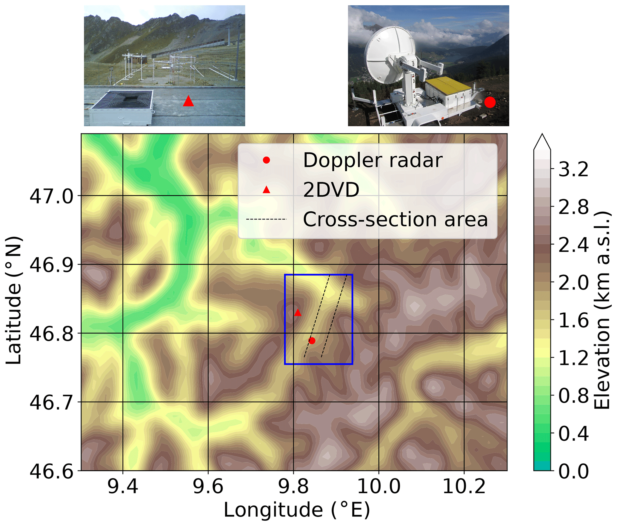
Figure 1 Overview of the model orography and the instrument location setup. The parallelogram (dashed black lines) is the domain of the flow-oriented vertical cross-section analysis in Sect. 3.1 following the direction of the dual-polarized Doppler radar MXPol (red dot located at 46.789^∘ N, 9.843^∘ E) data. The blue box is the domain used for analysis in Sect. 3.2 and 3.3. The red triangle is the location of the ground-based video disdrometer.

Simulations were conducted including several SIP processes, which consisted of ice–graupel collisions (as thoroughly discussed in Sect. 2.2.2 below) and a control simulation, referred to as the rime-splintering (RS) simulation, where only rime splintering was active. For each of these setups, five ensemble simulations are conducted by perturbing the initial temperature conditions at each grid point through the model domain with unbiased Gaussian noise at a zero mean and a standard deviation of 0.01 ^∘C (Selz and Craig, 2015; Keil et al., 2019). To account for the uncertainty associated with simulating atmospheric processes in mountainous terrain, three cross sections were interpolated from the model output (only the outer two cross sections are shown in Fig. 1). Each cross section, of which one cross section cuts more or less through the location of the radar, is separated by 1 km which is similar to the model resolution. The direction of each of the cross sections is similar to the direction of the generated RHI cross section from the weather radar. The three cross sections are then averaged and compared to the radar data. To generate the Hovmöller diagrams, we further took the mean along the length of the cross section for both the simulations and the radar data.

2.2.2 Cloud microphysics scheme

We use a detailed two-moment bulk cloud microphysics scheme within COSMO with six hydrometeor categories, including cloud droplets, rain, ice, snow, graupel and hail (Seifert and Beheng, 2006). The 2M scheme has been used extensively to study the evolution, lifetime, persistence and aerosol–cloud interactions of MPCs (Seifert et al., 2006; Baldauf et al., 2011; Lohmann et al., 2016; Possner et al., 2017; Henneberg, 2017; Glassmeier and Lohmann, 2018; Sullivan et al., 2018; Eirund et al., 2019, 2021). We refer to ice particles as any combination of the hail, graupel, snow or ice categories. Cloud droplet activation is based on an empirical activation spectrum which depends on the cloud-base vertical velocity and the prescribed number concentration of cloud condensation nuclei (Seifert and Beheng, 2006). The application is appropriate in atmospheric models with a horizontal grid size and time resolution of Δx≤1 km and Δt<10 s, respectively. The warm-phase autoconversion process from Seifert and Beheng (2001) was updated with the collision efficiencies from Pinsky et al. (2001) and also takes into account the decrease in terminal velocity associated with an increase in air density. A better approximation of the collision rate between hydrometeors was also introduced by Seifert and Beheng (2006), which makes use of the Wisner approximation (Wisner et al., 1972).

Primary production of ice occurs via homogeneous and heterogeneous nucleation pathways. Homogeneous freezing of cloud droplets, parameterized from the homogeneous freezing rates of Cotton and Field (2002), is calculated for $\mathrm{0}>T\ge -\mathrm{50}$ ^∘C. At −38 ^∘C most cloud droplets will freeze given the enhanced homogeneous nucleation rates at colder temperatures. As a lower bound, the homogeneous freezing of all cloud droplets occurs at $T=-\mathrm{50}$ ^∘C. The homogeneous nucleation of solution droplets, typically associated with cirrus cloud formation, follows Kärcher et al. (2006). Here, the number density and size of nucleated ice crystals are determined by the vertical wind speed, temperature and pre-existing cloud ice. Heterogeneous nucleation is empirically derived, which depends on the chemical composition and surface area of multiple species of aerosols, namely, organics, soot and dust (Phillips et al., 2008).

Table 1 Sensitivity settings for the collisional-breakup (BR) parameterization. The conversion rate (conv) is the size (in µm) at which rimed ice crystals or snowflakes are converted to graupel, α is the scale factor, F_BR is the fragments generated, and γ_BR is the decay rate of fragment number at warmer temperatures. When γ_BR=5, as used in the Takahashi parameterization (Sullivan et al., 2018), then T is included in the simulation name. The bold numbers represent the sensitivity simulations pertaining to the different conversion sizes of 300, 400 and 500 µm.

Secondary ice production through rime splintering, which is widely used in numerical weather prediction models, is the only process that is included in the standard version of COSMO (Blyth and Latham, 1997; Ovtchinnikov and Kogan, 2000; Phillips et al., 2006; Milbrandt and Morrison, 2016; Phillips et al., 2017). In COSMO, rime splintering occurs at $-\mathrm{3}\ge T\ge -\mathrm{8}$ ^∘C (Hallett and Mossop, 1974) when supercooled droplets and rain drops ($D_{\mathrm{c},\mathrm{r}}\ge \mathrm{25}$ µm) collide with ice hydrometeors ($D_{\mathrm{i},\mathrm{s},\mathrm{g}}\ge \mathrm{100}$ µm) (e.g., Seifert and Beheng, 2006). A default value of 350 fragments per milligram of rime is used in the rime-splintering parameterization. Another SIP process, collisional breakup, was added to COSMO and tested in several studies (Sullivan et al., 2018; Dedekind et al., 2021). Generally, collisional breakup refers to the collision of any two frozen hydrometeors with different densities in which the collisional kinetic energy is sufficient that the collisional impact causes shattering. Here, collisional breakup is when either ice or snow particles collide with graupel and fracture. This can increase the number of ice particles at temperatures warmer than −21 ^∘C. Almost no empirical constraint – apart from Takahashi et al. (1995), who used collisions between hail-sized particles – exists for the efficiency of any form of collisional breakup. The collisional kinetic energy and the density between hydrometeors are important parameters for this efficiency. In this study of the heavy snowfall event during which high K_dp values were recorded, we use the parameterizations for ice–graupel collisional breakup (BR) from Dedekind et al. (2021, BR28 and BR2.8T) and Sotiropoulou et al. (2021, BR-Sot) in COSMO in different forms:

$$\begin{array}{}\text{(4)}& {\displaystyle }\begin{array}{rl}& \mathrm{\aleph }{}_{\mathrm{BR}}={\displaystyle \frac{F_{\mathrm{BR}}}{\mathit{\alpha }}}(T-\mathrm{252}{)}^{\mathrm{1.2}}\exp \left[\begin{array}{c}-(T-\mathrm{252})/{\mathit{\gamma }}_{\mathrm{BR}}\end{array}\right]\\ & \text{for BR28}(F_{\mathrm{BR}},\mathit{\alpha },{\mathit{\gamma }}_{\mathrm{BR}})=(\mathrm{280},\mathrm{10},\mathrm{2.5}),\end{array}\text{(5)}& {\displaystyle }\begin{array}{rl}& \mathrm{\aleph }{}_{\mathrm{BR}}={\displaystyle \frac{F_{\mathrm{BR}}}{\mathit{\alpha }}}(T-\mathrm{252}{)}^{\mathrm{1.2}}\exp \left[\begin{array}{c}-(T-\mathrm{252})/{\mathit{\gamma }}_{\mathrm{BR}}\end{array}\right]\\ & \text{for BR2.8T}(F_{\mathrm{BR}},\mathit{\alpha },{\mathit{\gamma }}_{\mathrm{BR}})=(\mathrm{280},\mathrm{100},\mathrm{5}),\end{array}\text{(6)}& {\displaystyle }\begin{array}{rl}& \mathrm{\aleph }{}_{\mathrm{BR}}=F_{\mathrm{BR}}(T-\mathrm{252}{)}^{\mathrm{1.2}}\exp \left[\begin{array}{c}-(T-\mathrm{252}/{\mathit{\gamma }}_{\mathrm{BR}})\end{array}\right]{\displaystyle \frac{\stackrel{\mathrm{‾}}{D}}{{\stackrel{\mathrm{‾}}{D}}_{\mathrm{0}}}}\\ & \text{for BR-Sot}(F_{\mathrm{BR}},{\stackrel{\mathrm{‾}}{D}}_{\mathrm{0}},{\mathit{\gamma }}_{\mathrm{BR}})=(\mathrm{280},\mathrm{0.02},\mathrm{5}),\end{array}\end{array}$$

where ℵ_BR is the number of fragments generated per collision, α is the scale factor, F_BR is the leading coefficient, T is the temperature in kelvin, γ_BR is the decay rate of the fragment number at warmer temperatures, $\stackrel{\mathrm{‾}}{D}$ is the diameter of particles undergoing fracturing and ${\stackrel{\mathrm{‾}}{D}}_{\mathrm{0}}$ is the diameter of the hail particles used in Takahashi et al. (1995) (Table 1). Because of the inconsistency between the hail particles and their corresponding fall velocity used in Takahashi et al. (1995), which is described in more detail in Dedekind et al. (2021), all the parameterizations (Eqs. 4, 5 and 6) have scaling factors. Equations (4) and (5) were applied in Dedekind et al. (2021) for the BR28 and BR2.8T simulations, respectively. Equation (4) is scaled by α=10 and has a slower decay rate of fragment number at warmer temperatures represented by γ_BR=2.5, and Eq. (5) is scaled by 100 while using the same decay rate of fragment numbers of γ_BR=5 as used in Sullivan et al. (2018), which was derived from Takahashi et al. (1995) (Table 1). Equation (6), for the BR-Sot simulation, was applied in Sotiropoulou et al. (2021). They used a scaling parameter, $\stackrel{\mathrm{‾}}{D}/{\stackrel{\mathrm{‾}}{D}}_{\mathrm{0}}$, that was applied to the breakup parameterization from Sullivan et al. (2018) where ${\stackrel{\mathrm{‾}}{D}}_{\mathrm{0}}=\mathrm{0.02}$ m.

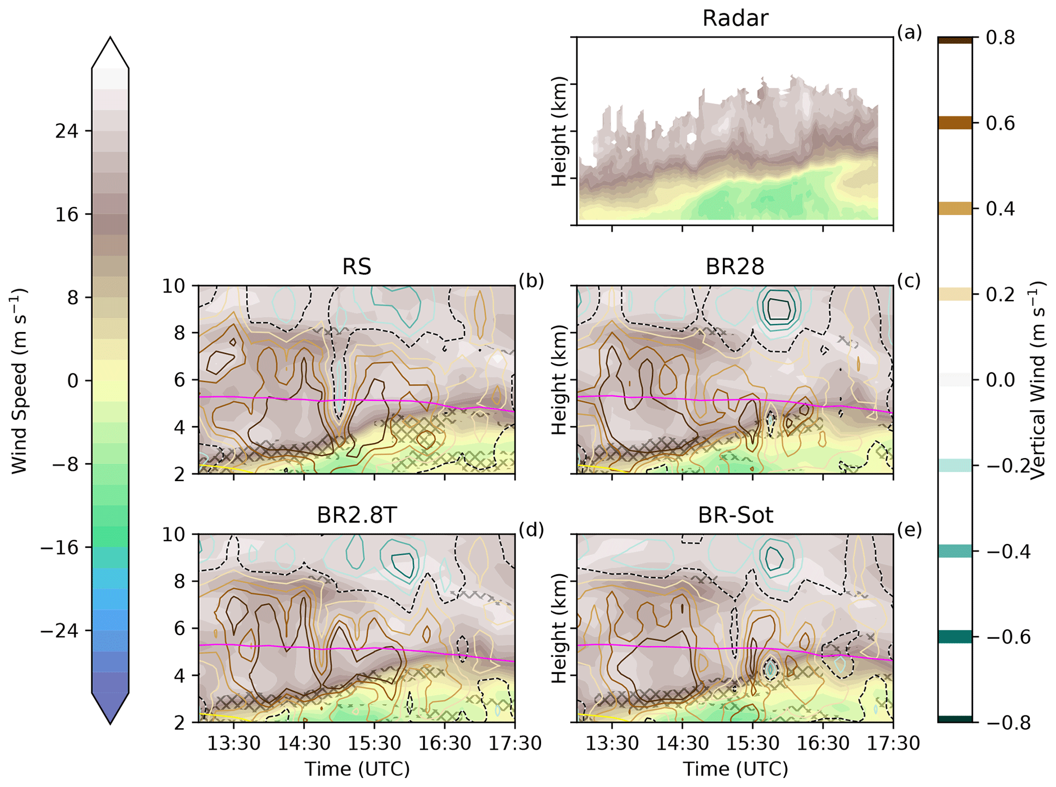
Figure 2 Hovmöller diagrams of wind speed and vertical velocity for panels (a) Doppler radar, (b) RS, (c) BR28, (d) BR2.8T and (e) BR-Sot between 13:00 and 17:30 UTC. The filled contours denote wind blowing towards (blue and green) and away (white and brown) from the radar, respectively. The pink line is the −21 ^∘C isotherm. At warmer temperatures collisional breakup occurs. Hatching denotes the region where the air layer is dynamically unstable, determined by a bulk Richardson number of less than 0.25.

Similar to Dedekind (2021), the ice crystal number concentration (ICNC) in COSMO is limited to 2000 L⁻¹. Furthermore, Dedekind (2021) concluded that the conversion rate from ice crystals or snow to graupel, which is a function of the riming rate of ice crystals or snow with raindrops, may contribute to enhanced collisional breakup (Seifert et al., 2006). In Eq. (70) of Seifert and Beheng (2006), they specify that ice and snow crystals can only be converted to graupel once they reach ${\stackrel{\mathrm{‾}}{D}}_{\mathrm{i},\mathrm{s}}\ge \mathrm{500}$ µm. However, in the current version of the 2M scheme (as used in this study), ice and snow crystals are converted to graupel already once they exceed ${\stackrel{\mathrm{‾}}{D}}_{\mathrm{i},\mathrm{s}}\ge \mathrm{200}$ µm. Therefore, earlier graupel formation is promoted in the current version, which should lead to enhanced SIP though ice–graupel collisions. To test the model's sensitivity to these different thresholds for graupel formation, we set up sensitivity studies with graupel formation at ${\stackrel{\mathrm{‾}}{D}}_{\mathrm{i},\mathrm{s}}\ge \mathrm{300}$, 400 and 500 µm to understand how the conversion rate impacts SIP processes. To accomplish this, we change the ice category conversion size requirement, ${\stackrel{\mathrm{‾}}{D}}_{\mathrm{i},\mathrm{s}}$, during riming from 200 µm (BR2.8T) to 300 µm (BR2.8T_300), 400 µm (BR2.8T_400) or lastly 500 µm (BR2.8T_500) (Table 1). The results of these sensitivity simulations can be found in Appendix C.

To investigate the impact of vertical wind shear and updraft on SIP, the probability density functions (PDFs) for the variables from the collisional-breakup simulations are analyzed. Furthermore, the joint PDFs are calculated along with the mutual information (MI, Shannon and Weaver, 1949) score, which quantifies the strengths of dependencies between the SIP rate and cloud properties (e.g., Dawe and Austin, 2013). For this purpose, a 10 km × 10 km region was selected and masked by the levels in which SIP occurred ($T>-\mathrm{21}$ ^∘C, blue box in Fig. 1) from 15:15 to 16:30 UTC. This resulted in the 16 121 data points for which an expression from Hacine-Gharbi et al. (2013) was used for finding the optimal number of bins (17 bins in our case) to estimate the MI for continuous random variables.

3 Results

3.1 The case study

A synoptic system passed over Switzerland on 26 March 2010, during which we analyzed the evolution of a cold front from 13:00 to 17:30 UTC with intense precipitation from 15:00 to 17:30 UTC. Furthermore, the cold front was associated with a surface temperature drop of ∼7 ^∘C (Fig. S1 in the Supplement), a southwesterly wind flow at higher altitudes, vertical wind shear closer to the surface below 4 km a.m.s.l. and the development of peculiar polarimetric radar signatures. In particular, K_dp reached values around 1.5^∘ km⁻¹ at certain height levels, and towards the end of the event it was exceeding 2^∘ km⁻¹ (Fig. 3a). A statistical analysis of K_dp in snowfall conducted with this radar and in this location over a long observation period (Schneebeli et al., 2013) showed that the 80th percentile of K_dp at every height level is lower than 0.5^∘ km⁻¹. Considering that the distribution of K_dp is very skewed, values above 1^∘ km⁻¹ in snow can be considered unusually large.

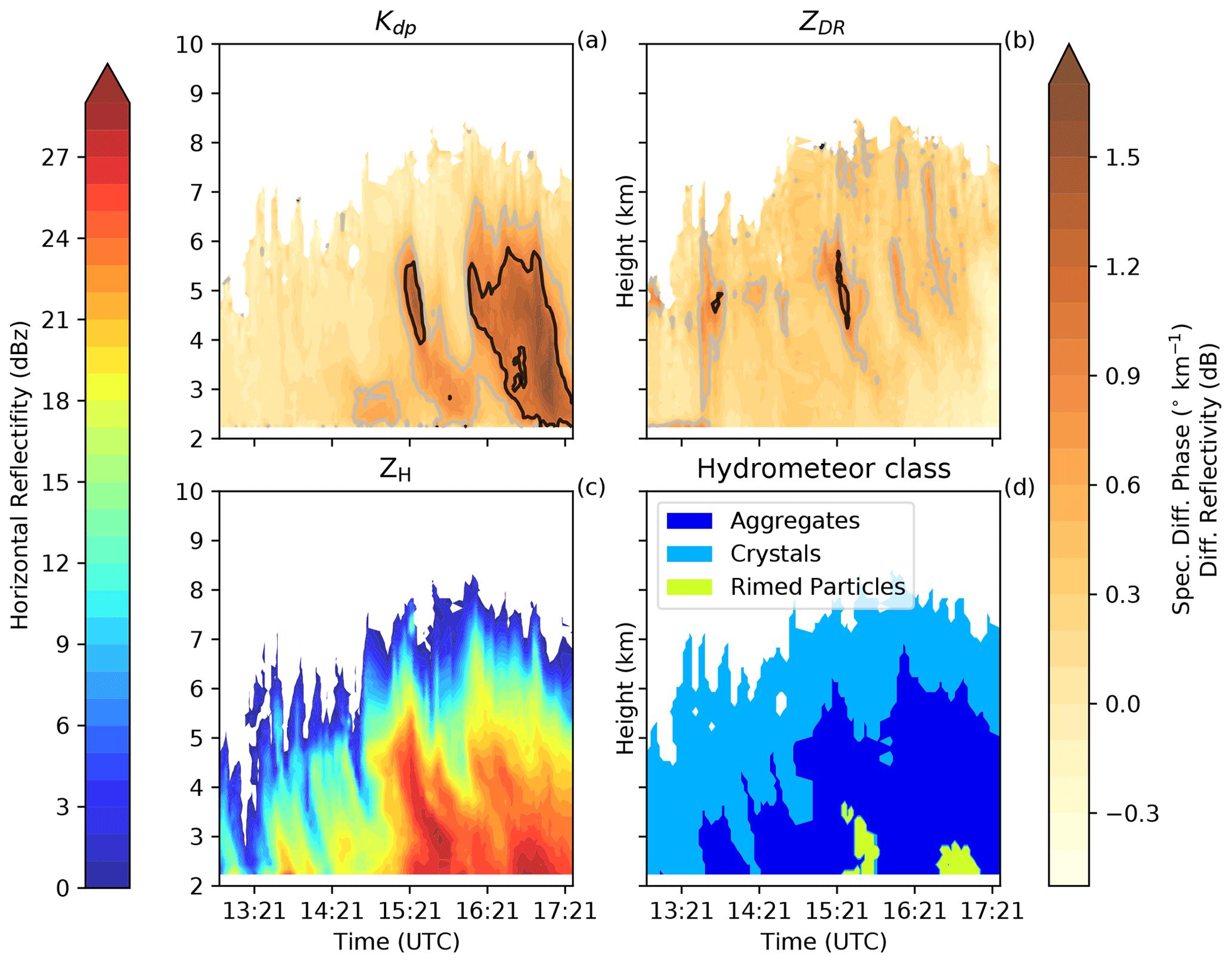
Figure 3 Hovmöller diagrams of the (a) spectral differential phase (K_dp), the (b) differential reflectivity (Z_DR), (c) the horizontal reflectivity (Z_H) and (d) the hydrometeor class categories derived from the Doppler radar between 13:00 and 17:30 UTC. The gray and black lines in panels (a) and (b) are where both K_dp and Z_DR are larger than 0.5 and 1, respectively.

Wind shear, observed by the dual-polarization Doppler radar, was visible between 2 and 5 km a.m.s.l. (Fig. 2a). The wind velocity at lower altitudes shifted from southerly to northerly, which was captured in all simulations, albeit not as prominent as the observations (Figs. 2b–e). The wind shear and the associated updrafts may have contributed to an enhanced SIP rate between 3 and 5 km in the collisional-breakup simulations (Fig. 2c–e). Here, the bulk Richardson number, which is a ratio of the buoyant energy to shear-kinetic energy, is determined to assess the dynamic stability of the air layer. An air layer becomes turbulent if the Richardson number is less than the critical Richardson number of 0.25 (e.g., Stull, 2016). Figure 2b–e shows where the air layer was turbulent with enhanced interactions between ice particles that could have caused enhanced ice–graupel collisions. Regions of enhanced updraft, where hydrometeors can grow to larger sizes, were mostly seen immediately above the turbulent layer.

The subzero temperature in the region of enhanced K_dp was warmer than −21 ^∘C, which is in the temperature range favorable for ice–graupel collisions (Takahashi et al., 1995). We thus hypothesize that the in situ cloud conditions together with the vertical wind shear could have triggered higher secondary ice production rates that can be reflected in radar measurements, as K_dp is a possible indicator of high number concentrations of oblate hydrometeors in the radar sampling volume (Kennedy and Rutledge, 2011; Bechini et al., 2013; Grazioli et al., 2015a; von Terzi et al., 2022).

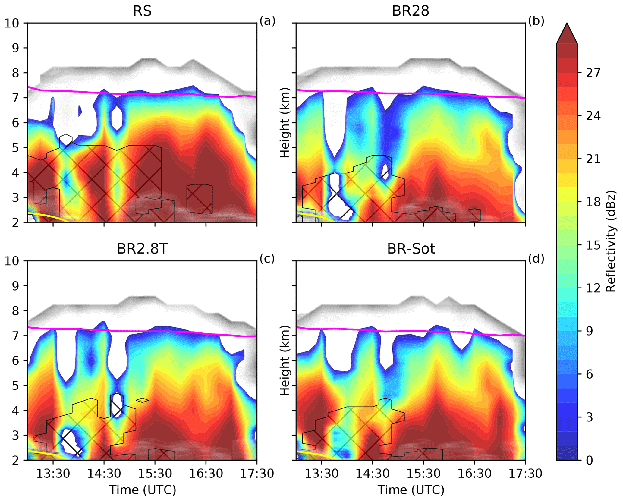
Figure 4 Hovmöller diagrams of the simulated reflectively for panels (a) RS, (b) BR28, (c) BR2.8T and (d) BR-Sot between 13:00 and 17:30 UTC. The hatched area is defined as the MPC where the cloud droplet mass concentration and ice mass concentration are greater than 10 and 0.1 mg m⁻³, respectively. The pink line is the homogeneous freezing line at −38 ^∘C, and the shaded gray area is the cloud area fraction.

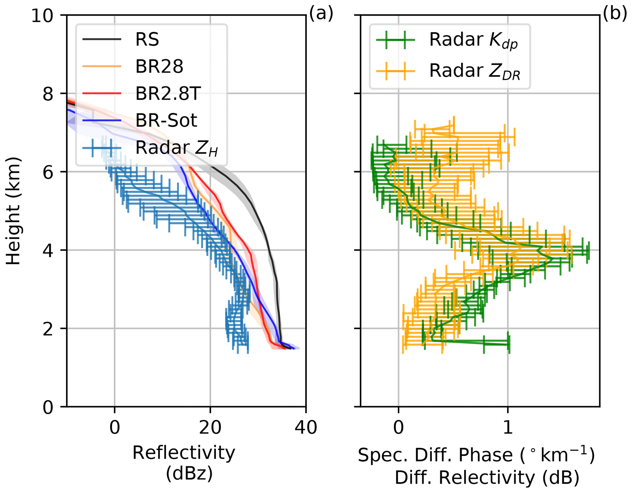
Figure 5 Vertical profiles of the (a) horizontal reflectivity (Z_H), (b) specific differential phase (K_dp) and differential reflectivity (Z_DR). The solid lines are the mean, with shaded areas and error bars showing the 10th and 90th percentiles for the model simulations and Doppler radar, respectively, at 15:30 UTC.

3.2 Simulated vs. observed radar reflectivity

3.2.1 Model and Doppler radar comparison

Horizontal reflectivity Z_H is used to compare the model to the observations throughout the cloud and to analyze the impact of secondary ice production on the simulated radar reflectivity. During the early afternoon, the median of Z_H remained mostly below 20 dBz. At around 15:15 UTC larger ice hydrometeors were present (either as a result of enhanced aggregation or depositional growth) between 4 and 6 km a.m.s.l., which then started to sediment (Fig. 3c and d). A peak in Z_H at 3 km a.m.s.l. was observed in the fall streaks when the cloud droplets rimed onto the sedimenting ice hydrometeors. The RS simulation overestimated Z_H by at least 8 dBz throughout the vertical profile at 15:30 UTC, while all the collisional-breakup simulations captured Z_H more accurately, especially between 3 and 5 km a.m.s.l. (Figs. 4 and 5a). The radar-derived hydrometeor classification showed that much of the ice hydrometeor growth occurred through aggregation and riming. At 15:30 UTC, very high median K_dp>1^∘ km⁻¹ and Z_DR>1 dB were observed (Fig. 5b). The vertical evolution of K_dp and Z_DR is similar, with a peak observed about 4 km a.m.s.l., which is 1 km above the peak in Z_H (Fig. 5b). The large and colocated values of Z_DR and K_dp suggest that a large population of oblate and rimed particles, without a significant presence of large isotropic hydrometeors, was present.

Later, during the event (Fig. 3) the peak of Z_DR was more often above the peak of K_dp, suggesting that the population of particles in the areas of enhanced K_dp also included larger isotropic aggregates. The occurrence of peaks in polarimetric variables at certain heights above ground (K_dp in particular) has been observed during intense snowfall events (e.g., Kennedy and Rutledge, 2011; Schneebeli et al., 2013; Grazioli et al., 2015a). The K_dp enhancement in particular has often been observed near the −15 ^∘C isotherm and has been interpreted as the signature of enhanced dendritic growth (Kennedy and Rutledge, 2011; Bechini et al., 2013) in combination with secondary ice production (von Terzi et al., 2022). Dendrites are prone to aggregation; therefore, the K_dp peak disappears (and Z_H increases) as particles approach the ground level.

Figure 6 Vertical profiles for the (a) ice number concentration (NICE), (b) secondary ice production (SIP) and (c) ice water content (IWC). The solid lines are the mean, with shaded areas and error bars showing the 10th and 90th percentiles for the model simulations and Doppler radar, respectively, at 15:30 UTC. The green triangle is the 2DVD surface observations for hydrometeors D>0.2 mm.

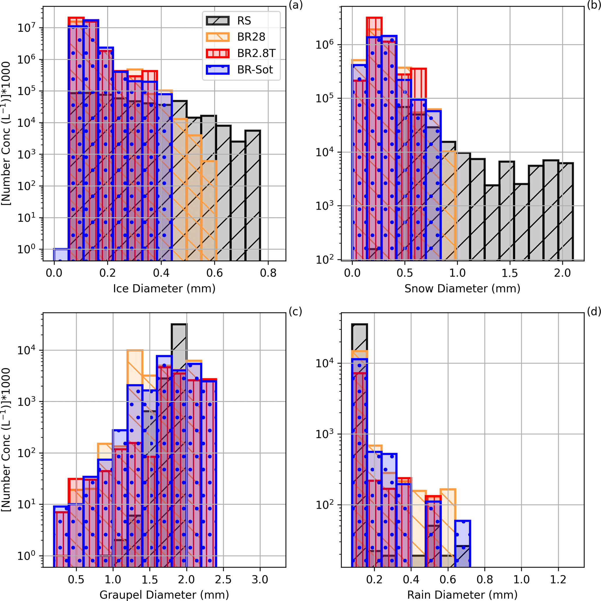
Figure 7 Particle size distribution for panels (a) ice, (b) snow, (c) graupel and (d) raindrops for all the simulations at 15:30 UTC.

Figure 8 Hovmöller diagrams of graupel and rain mixing ratio for panels (a) RS, (b) BR28, (c) BR2.8T and (d) BR-Sot between 13:00 and 17:30 UTC. The hatched area is defined as the MPC where the cloud droplet mass concentration and ice mass concentration are greater than 10 and 0.1 mg m⁻³, respectively. The pink line is the homogeneous freezing line at −38 ^∘C, and the shaded gray area is the cloud area fraction.

3.2.2 Modeled and measured cloud properties

Throughout the vertical profile below 6 km at 15:30 UTC, the ice crystal number concentration was at least an order of magnitude larger than expected from the RS simulation with a SIP rate in excess of 20 L⁻¹ s⁻¹ (Fig. 6). In both Figs. 6 and S2 the observed ice crystal number concentration recorded by the disdrometer (∼20 L⁻¹) was remarkably well represented at the surface by the BR2.8T and BR-Sot simulations (similar results are shown in Dedekind et al., 2021). The ice crystal and snow number concentrations were orders of magnitudes larger for ${\stackrel{\mathrm{‾}}{D}}_{\mathrm{i}}<\mathrm{0.4}$ mm and ${\stackrel{\mathrm{‾}}{D}}_{\mathrm{s}}<\mathrm{0.8}$ mm, respectively, compared to the RS simulation (Fig. 7a and b).

During the late stage of the snowfall event, at 17:00 UTC, the replenishment of graupel diminished rapidly (Figs. 8 and S2c), causing a substantial reduction in the SIP rate (Fig. S2). Less collisional breakup allowed the ice and snow crystals to grow to larger sizes, ${\stackrel{\mathrm{‾}}{D}}_{\mathrm{i}}\sim \mathrm{1.2}$ mm and ${\stackrel{\mathrm{‾}}{D}}_{\mathrm{s}}\sim \mathrm{3.3}$ mm, respectively, primarily through deposition and/or aggregation (Fig. S3a and b). A lower Z_DR is consistent with less anisotropic particles produced by aggregation and/or riming. However, the enhanced concentration of oblate particles (increase in K_dp) was in contrast to the simulations, showing a reduction in cloud content as the cloud began to dissipate earlier than in the observations. None of the simulations were able to describe the high ice particle formation event that was most likely triggered through ice–ice collisions of aggregates of dendrites given the favorable temperature range.

3.2.3 Microphysical explanations

Z_H was significantly overestimated by the RS simulation between 13:00 and 17:30 UTC, which most likely was a result of the following chain of events. (1) Insufficient droplets of size 25 µm (Fig. 7d), within the narrow temperature range ($-\mathrm{3}\ge T\ge -\mathrm{8}$ ^∘C), led to a limitation in ice particle growth by riming and therefore limited rime splintering (Fig. 6b). (2) Because rime splintering was not that active, typical for wintertime MPCs (e.g., Henneberg et al., 2017; Dedekind et al., 2021), the ice and snow crystals grew mainly by depositional growth and aggregation. (3) The ice and snow crystal size distributions widened substantially (Figs. 7a, b and S3a, b). Both of these categories had number concentrations of less than 100 L⁻¹ with particle diameters of up to 0.8 and 5.1 mm, respectively, at 15:30 UTC. (4) The larger ice and snow crystal diameters resulted in enhanced Z_H. These observations are consistent with other times during the day which showed even larger-sized ice and snow crystals of 0.9 and 5.2 mm, respectively (Figs. S4a and S5a), as well as higher rain mass mixing ratios (e.g., Fig. 8a). There were single grid points where snowflakes even reached diameters of 13 to 17 mm during the latter part of the day (not shown here). Additionally, excessive size sorting in the model most likely contributed to the overestimation in Z_H. Size sorting typically occurs within the sedimentation parameterization of 2M schemes in regions of vertical wind shear or updraft cores (Milbrandt and McTaggart-Cowan, 2010; Kumjian and Ryzhkov, 2012). All these factors contributed to the RS simulation overestimating Z_H compared to the observations (Fig. 5a).

When collisional breakup was allowed to occur in the BR28, BR2.8T and BR-Sot simulations, the ice and snow crystals did not have time to grow as large compared to the ice and snow crystals in the RS simulation. The smaller ice particles were associated with a reduced Z_H which compared better to the observations than the RS simulations.

Comparing the collisional-breakup simulations showed that the BR28 simulation still generated 8 times more ice particles than the BR2.8T and BR-Sot simulations at 4 km a.m.s.l. at $T\approx -\mathrm{15}$ ^∘C (Fig. 6b). At temperatures of −10 ^∘C (3 km a.m.s.l.), the SIP rate decreased rapidly from 100 L⁻¹ s⁻¹ to almost 0 L⁻¹ s⁻¹ at the surface. The lower SIP rates (less ice–graupel collisions) compared to the BR2.8T and BR-Sot simulations had several implications: (1) ice crystals and snow particles had more time to grow to larger sizes as seen in the wider particle size distributions (Fig. 7); (2) the number of ice hydrometeors was an order of magnitude below (worst in the collisional-breakup simulations) the observed ground-based video disdrometer observations of ∼20 L⁻¹ (for particles less than 0.2 mm) at 15:30 and 17:00 UTC (Figs. 6a and S2c); and (3) interestingly, the simulated Z_H compared slightly better with the radar observations, although the ice hydrometeors were overestimated (Figs. 5a, 6a, S2c and S2d). Because the BR2.8T and BR-Sot simulations showed similar results, which were better than the BR28 simulation, only the BR2.8T simulation is used in the next section to link the simulated wind shear to SIP.

3.3 Linking simulated wind shear to SIP

In this section, the dependence of the SIP rate on wind patterns is examined over the region (blue box) depicted in Fig. 1 during three time periods: 13:00–14:15 UTC (early, Fig. S6), 14:30–15:45 UTC (middle, Fig. 9) and 16:00–17:15 UTC (late, Fig. S7). The early period was categorized with strong wind shear and a turbulent layer below 3 km (Fig. 2a–e). During the middle period, the turbulent layer extended to 4 km during which graupel increased in the MPC. The late period was categorized by less wind shear, causing the dissipation of the turbulent layer. The cloud entered a glaciated state during this time. We analyzed the middle period as it was the most important period, according to the model, in terms of SIP and is therefore shown in Fig. 9. Regions in which SIP did not occur (e.g., $T<-\mathrm{21}$ ^∘C) were masked out for this analysis.

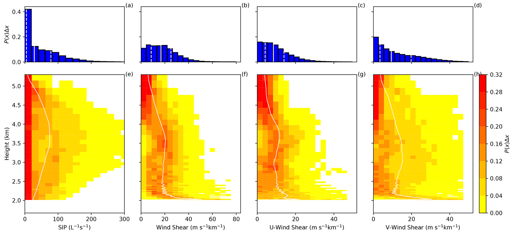
Figure 9 Probability density functions of different variables (P(x)) from the BR2.8T simulation from all model levels (top row) and at each model level (bottom row) for (a, e) secondary ice production (SIP) rate, (b, f) wind shear, (c, g) U-wind shear and (d, h) V-wind shear between 14:30–15:45 UTC. The solid and dashed white lines are the horizontal 50th percentile and the 25th and 75th percentiles, respectively, of each variable over the 10 km×10 km domain.

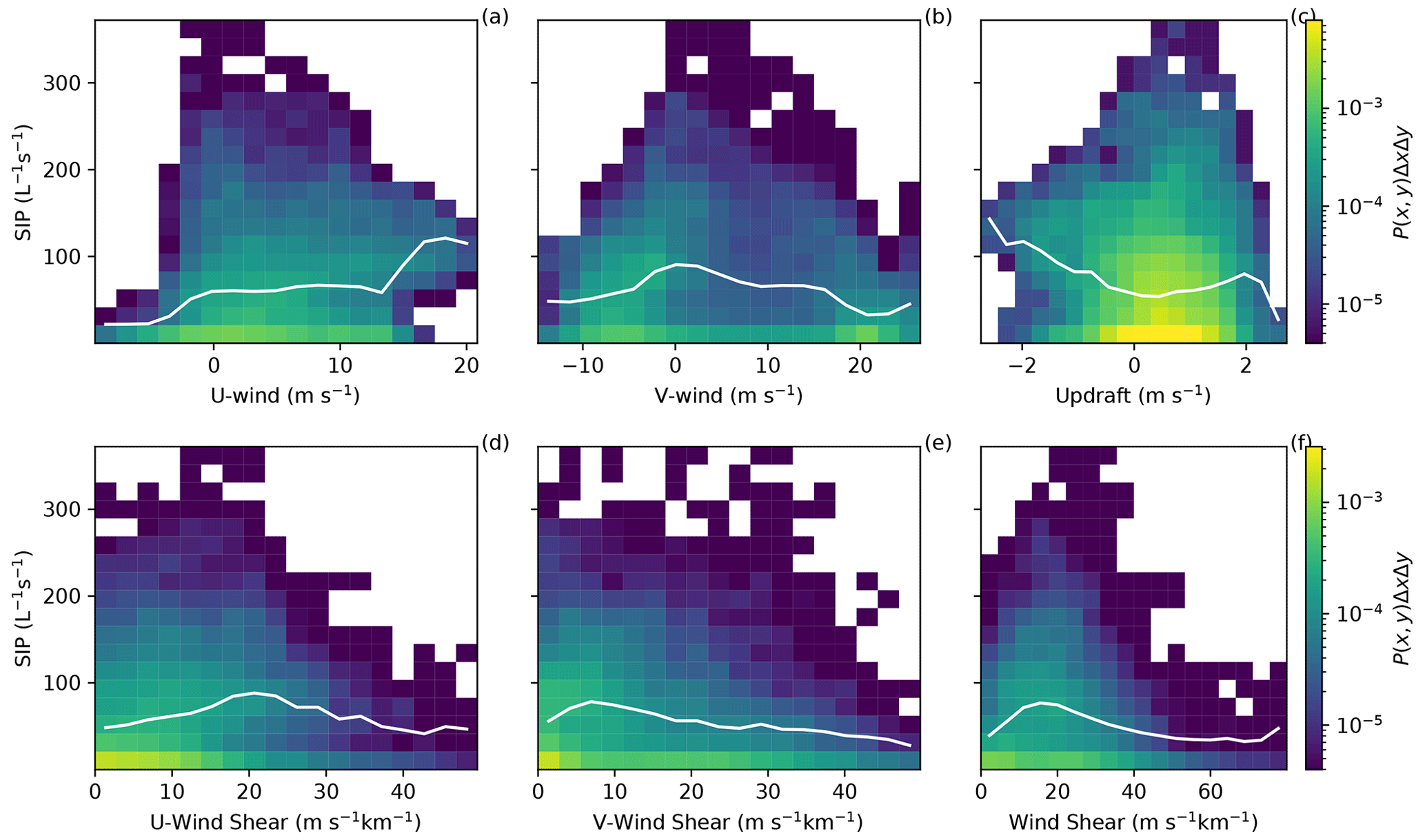
Figure 10 Joint probability density function multiplied by bin area (P(x,y)ΔxΔy) for the model output of SIP versus (a) U wind, (b) V wind, (c) updraft, (d) U-wind shear, (e) V-wind shear and (f) wind shear for the BR2.8T simulation. White lines are the 50th percentile as a function of the x-axis variable.

Figure 11 Normalized median values of the PDFs of the variables in Table 2 for the three different time periods for the BR2.8T simulation.

A strong shift between the early and middle period in the V-wind median and interquartile range occurred from 20.5 to −0.7 m s⁻¹ and 6.6 to 21.3 m s⁻¹, respectively, compared to the U wind (Table 2). In fact, the U wind had a small variability between the early and middle periods (Table 2). As the afternoon progressed, the median of the strongest V-wind shear extended from near the surface at 14:30 to 5 km a.m.s.l. at 16:30 UTC (Figs. 2 and 9). Updraft cells developed above this level of strong vertical wind shear between 10 and 20 m s⁻¹ km⁻¹. Our observation is consistent with Houze and Medina (2005) and Medina and Houze (2015), who also showed that updraft cells occurred at times and locations where the shear was strongest ($>\sim \mathrm{10}$ m s⁻¹ km⁻¹). During the middle time period, the variability in the V-wind shear was the largest with an interquartile range of 16.3 m s⁻¹ km⁻¹, which coincided with the highest SIP rate (Fig. 9d and Table 2). The joint probability density functions (PDFs) (P(SIP rate, V-wind shear)) illustrate that the correlation median between the V-wind shear and SIP rate peaked at 9 m s⁻¹ km⁻¹ and 80 L⁻¹ s⁻¹ (Fig. 10e). This peak coincided with the region where the wind shifted from southwesterly to northerly (along the valley) between the early and middle periods. This shift was a result of the change in the V-wind speed from negative to positive at 2.9 km a.m.s.l. The joint PDF between the V wind and SIP (Fig. 10b) was highest at this altitude. Here, an environment of stronger meridional wind shear tends to coincide with the environment for high secondary ice production (Fig. 10f and Table 2).

The contribution of the updraft velocity to SIP is not as clear. The increase (early to middle period) and decrease (middle to late period) of the median of the SIP rates poorly co-varied with the U-wind shear or updraft compared to the V-wind shear (Fig. 11).

Table 2 The 25th, 50th and 75th percentiles and the interquartile range (IQR) between the 10th and 90th percentiles of the vertical profiles for the BR2.8T simulations.

To further highlight this role, we calculated the mutual information shared between different sets of variables. The mutual information (MI: I(X;Y)) between variables X and Y was further analyzed for non-linear relationships (Shannon and Weaver, 1949), where X∈ [SIP rate] and Y∈ [U wind, V wind, updraft, U-wind shear, V-wind shear, wind shear]. I(X;Y)) of 0 bits means no information is shared between X and Y; therefore, Y cannot be inferred from X. (Further information about MI can be found in Appendix A and also in Dawe and Austin (2013).) For instance, during the last period the relationship of I(SIP rate; wind shear) weakened drastically to 0.021 bits to below the level of significance (Table 3) compared to earlier periods. This was expected as the diminishing cloud liquid water caused a reduction in the riming rates. Lower riming rates limited graupel formation which in turn reduced ice–graupel collisions.

The significantly higher MI score between I(SIP rate; wind shear) during the early and middle periods was a result of the strengthening of the northerly valley winds during the early afternoon hours when the predominant wind aloft was southwesterly (generating the dominant V-wind shear). The development of the northerly winds could have been a result of low-level blocking that generated the shear layer (Medina et al., 2005). The sharp change in the wind speed and direction enhanced the turbulent overturning and therefore promoted the riming of ice crystals and snow, leading to the formation of graupel which in turn enhanced the SIP rates. The higher MI score between I(SIP rate; wind shear) implies there is a stronger relationship between wind shear and SIP than the other variables analyzed here.

Table 3 Mutual information between SIP rate and wind properties of the vertical profiles for the BR2.8T simulations. The significance level is calculated by taking the maximum of 1000 Monte Carlo simulations of mutual information between a random permutation of SIP rates and each variable.

4 Conclusions

A cold front passage on 26 March 2010, over the Swiss Alps, associated with strong vertical wind shear and intense polarimetric signatures was observed with a dual-polarization Doppler weather radar deployed at Davos. This study investigates the role of vertical wind shear on the rate of SIP by making simulations of wintertime orographic MPCs with a non-hydrostatic, limited-area model, COSMO, which has a two-moment bulk microphysics scheme with six hydrometeor categories, as well as two additional parameterizations for ice–graupel collisions (e.g., Sotiropoulou et al., 2020; Dedekind, 2021) based on Takahashi et al. (1995). To conclude, our main findings can be summarized as follows:

• Large values of K_dp>1^∘ km⁻¹ suggest that a large population of oblate particles was present, most likely originating from ice–ice collisions, at 4 km a.m.s.l. This level coincided with the −15 ^∘C isotherm. At −15 ^∘C dendritic growth is very fast, causing low-density dendrites to fracture and aggregate. At this time, Z_DR was also positive, indicating that large isotropic particles were less present. At lower altitudes, Z_H increased while K_dp (and Z_DR) decreased, suggesting aggregation and/or riming were occurring.

• The rime-splintering simulations overestimated Z_H throughout the vertical profile and underestimated the disdrometers’ number concentration of hydrometeors at the surface. Both shortcomings could be explained by omission of ice–graupel collisions.

• The breakup simulations (BR28, BR2.8T and BR-Sot) caused narrower ice crystal and snow distributions (enhanced number concentrations of smaller ice particles), resulting in a better representation of Z_H. The enhanced number concentrations of ice particles meant that these simulations, in particular BR2.8T and BR-Sot, captured the disdrometer observations of ∼20 L⁻¹ (considering the 0.2 mm observation limit) at 15:30 and 17:00 UTC.

• During the middle period, 14:30–15:45 UTC, the V-wind shear increased by 60 %, causing conditions favorable for accretion and leading to enhanced graupel formation and SIP in the region favorable for SIP.

• Another time period with high K_dp but low Z_DR was observed at 17:00 UTC, which was not captured by the breakup simulations as the graupel mixing ratio was depleted. The breakup parameterization does not include ice–ice collisions and relies only on graupel as the colliding species. At this time, the radar signatures suggested that collisions of dendrites caused the formation of small oblate particles (increasing K_dp) but also the formation of a few, larger, isotropic aggregates (decreasing Z_DR).

• The mutual information between the SIP rate and other variables like vertical wind shear and updraft velocity suggested that the SIP rate is best predicted by the overall wind shear.

• The sensitivity of the ice–graupel simulations to the conversion rate size restriction was measured using the Kullback–Leibler divergence. The sensitivity simulations were not sensitive to the conversion rate size thresholds.

Turbulent overturning, whether it is associated with baroclinic waves (Gehring et al., 2020) or low-level blocking (Medina et al., 2005; Houze and Medina, 2005; Medina and Houze, 2015), has been shown to play an important role in accreting hydrometeors to form precipitation. Here, we considered that the interactions of ice hydrometeors can lead to ice–graupel collisions, causing enhanced small ice fragments, as opposed to only growing larger through aggregation. These smaller fragments fall slower against updraft and may decrease local precipitation rates, enhancing precipitation downstream of the flow (Dedekind et al., 2021). Wind shear plays a significant role in ice–graupel collisions and may even be more important when all ice–ice collisions are considered in more physically robust collisional-breakup parameterizations (Yano and Phillips, 2011; Phillips et al., 2017). By only considering ice–graupel collisions, we are limited to mainly investigating collisional breakup in MPCs where riming can occur to form graupel. In the case where a cloud becomes glaciated and graupel cannot form through riming, our parameterization will not be able to simulate SIP, which may still prove to be very important.

Appendix A: Derivation of the simulated radar reflectivity

Here we briefly show the calculation of the simulated Z_H (Appendix B, Seifert, 2002). Calculating Z_H from the two-moment cloud microphysics scheme would not be possible without approximations and assumptions. The following relationship for the radar reflectivity of drops (Z_w), using the Rayleigh approximation for the cross section of drops (Eq. A1), results in

$$\begin{array}{}\text{(A1)}& {\mathit{\eta }}_{\mathrm{w}}={\displaystyle \frac{{\mathit{\pi }}^{\mathrm{5}}{\left|K_{\mathrm{w}}\right|}^{\mathrm{2}}}{{\mathit{\lambda }}_R^{\mathrm{4}}}}\underset{\mathrm{0}}{\overset{\mathrm{\infty }}{\int }}{D}^{\mathrm{6}}{f}_{\mathrm{w}}\left(D\right)\mathrm{d}D,\end{array}$$

where D is the particle diameter, λ_R is the wavelength of radar radiation, η_w is the volumetric liquid water content, f_w(D) is the number density distribution function for liquid water and $K_{\mathrm{w}}^{\mathrm{2}}=\mathrm{0.93}$ is the dielectric constant of liquid water. The reflectivity factor for cloud water is given by the following:

$$\begin{array}{}\text{(A2)}& \begin{array}{rl}{\stackrel{\mathrm{̃}}{Z}}_{\mathrm{w}}& ={\displaystyle \frac{{\mathit{\lambda }}_R^{\mathrm{4}}}{{\mathit{\pi }}^{\mathrm{5}}{\left|K_{\mathrm{w}}\right|}^{\mathrm{2}}}}{\mathit{\eta }}_{\mathrm{w}}=\underset{\mathrm{0}}{\overset{\mathrm{\infty }}{\int }}{D}^{\mathrm{6}}{f}_{\mathrm{w}}\left(D\right)\mathrm{d}D\\ & ={\left({\displaystyle \frac{\mathrm{6}}{\mathit{\pi }{\mathit{\rho }}_{\mathrm{w}}}}\right)}^{\mathrm{2}}\underset{\mathrm{0}}{\overset{\mathrm{\infty }}{\int }}{x}^{\mathrm{2}}{f}_{\mathrm{w}}\left(x\right)\mathrm{d}x={\left({\displaystyle \frac{\mathrm{6}}{\mathit{\pi }{\mathit{\rho }}_{\mathrm{w}}}}\right)}^{\mathrm{2}}{Z}_{\mathrm{w}},\end{array}\end{array}$$

where ρ_w is the water density. Because of the backscatter behavior for the mass-equivalent diameter with regards to ρ_w and ρ_i (ice density), the same applies to graupel, which is described as a spherical ice particle

$$\begin{array}{}\text{(A3)}& {\mathit{\eta }}_{\mathrm{g}}={\displaystyle \frac{{\mathit{\pi }}^{\mathrm{5}}{\left|K_{\mathrm{i}}\right|}^{\mathrm{2}}}{{\mathit{\lambda }}_R^{\mathrm{4}}}}{\left({\displaystyle \frac{\mathrm{6}}{\mathit{\pi }{\mathit{\rho }}_{\mathrm{i}}}}\right)}^{\mathrm{2}}\underset{\mathrm{0}}{\overset{\mathrm{\infty }}{\int }}{x}^{\mathrm{2}}{f}_{\mathrm{g}}\left(x\right)\mathrm{d}{x}_{\mathrm{1}},\end{array}$$

where x is the particle mass, f_g(x) is the number density distribution function for graupel and $K_{\mathrm{i}}^{\mathrm{2}}=\mathrm{0.176}$ is the dielectric constant of ice. The radar reflectivity factor for ice particles (e.g., graupel) is given by the following:

$$\begin{array}{}\text{(A4)}& \begin{array}{rl}{\stackrel{\mathrm{̃}}{Z}}_{\mathrm{g}}& ={\displaystyle \frac{{\mathit{\lambda }}_R^{\mathrm{4}}}{{\mathit{\pi }}^{\mathrm{5}}{\left|K_{\mathrm{w}}\right|}^{\mathrm{2}}}}{\mathit{\eta }}_{\mathrm{g}}={\displaystyle \frac{{\left|K_{\mathrm{i}}\right|}^{\mathrm{2}}}{{\left|K_{\mathrm{w}}\right|}^{\mathrm{2}}}}{\left({\displaystyle \frac{\mathrm{6}}{\mathit{\pi }{\mathit{\rho }}_{\mathrm{i}}}}\right)}^{\mathrm{2}}\underset{\mathrm{0}}{\overset{\mathrm{\infty }}{\int }}{x}^{\mathrm{2}}{f}_{\mathrm{g}}\left(x\right)\mathrm{d}x\\ & ={\displaystyle \frac{{\left|K_{\mathrm{i}}\right|}^{\mathrm{2}}}{{\left|K_{\mathrm{w}}\right|}^{\mathrm{2}}}}{\left({\displaystyle \frac{\mathrm{6}}{\mathit{\pi }{\mathit{\rho }}_{\mathrm{i}}}}\right)}^{\mathrm{2}}{Z}_{\mathrm{g}}.\end{array}\end{array}$$

For melting ice particles, however, K_w must be used instead of K_i. In our study, the surface and in situ cloud temperatures were below 0 ^∘C. More information on the reflectivity calculations for melting ice particles can be found in Seifert (2002, Appendix B). Finally, the radar reflectivity factor is given by

$$\begin{array}{}\text{(A5)}& \text{dBZ}={\displaystyle \frac{\mathrm{10}}{\ln \mathrm{10}}}\ln \left[{\displaystyle \frac{Z_{\mathrm{radar}}}{{\mathrm{mm}}^{\mathrm{6}}{\mathrm{m}}^{-\mathrm{3}}}}\right],\end{array}$$

where Z_radar is the sum of the reflectivity calculated for each individual cloud particle category (e.g., cloud drops, raindrops, ice crystals, snow crystals, graupel and hail):

$$\begin{array}{}\text{(A6)}& Z_{\mathrm{radar}}={\left({\displaystyle \frac{\mathrm{6}}{\mathit{\pi }{\mathit{\rho }}_{\mathrm{w}}}}\right)}^{\mathrm{2}}\left[Z_{\mathrm{c}}+Z_{\mathrm{r}}+{\displaystyle \frac{{\mathit{\rho }}_{\mathrm{w}}^{\mathrm{2}}}{{\mathit{\rho }}_{\mathrm{i}}^{\mathrm{2}}}}{\displaystyle \frac{\left|K_{\mathrm{i}}^{\mathrm{2}}\right|}{\left|K_{\mathrm{w}}^{\mathrm{2}}\right|}}\left(Z_{\mathrm{ic}}+Z_{\mathrm{s}}+Z_{\mathrm{g}}\right)\right].\end{array}$$

Appendix B: Mutual Information

The entropy H of the variable x's probability density function P(x) is defined by Shannon and Weaver (1949) to be

$$\begin{array}{}\text{(B1)}& H=-\int P\left(x\right)\ln \left(P\right(x\left)\right)\mathrm{d}x,\end{array}$$

where x is the information content of a single measurement of $P\left(x\right)=-\ln P\left(x\right)$. The entropy is a measure of the amount of information that is required to represent the PDF. From here, both the Kullback–Leibler divergence and the mutual information can be calculated.

The Kullback–Leibler divergence, also known as the relative entropy, measures the distance between two probability distributions, P(x) and Q(x), over a discrete random variable X. The Kullback–Leibler divergence is defined as follows:

$$\begin{array}{}\text{(B2)}& D_{\mathrm{KL}}(P\parallel Q)=\int P\left(x\right)\ln \left({\displaystyle \frac{P\left(x\right)}{Q\left(x\right)}}\right)\mathrm{d}x.\end{array}$$

The mutual information (MI) is a measure of the mutual dependence between two random variables X and Y (e.g., the entropy of X subtracted from the entropy of X conditioned on Y):

$$\begin{array}{}\text{(B3)}& I(X;Y)=H\left(X\right)-H\left(X\right|Y).\end{array}$$

MI describes, therefore, how different the joint distribution of the pair (X, Y) is from the distribution of X and Y. Combining Eqs. (B1) and (B3) yields

$$\begin{array}{}\text{(B4)}& I(X;Y)=\int \left[P\right(x\left)\ln \right(P\left(x\right))-P(x,y\left)\ln \right(P\left(x\right|y\left)\right)]\mathrm{d}x\mathrm{d}y,\end{array}$$

and because $P\left(x\right|y)=P(x,y)/P(y)$, Eq. (B5) can be reduced to

$$\begin{array}{}\text{(B5)}& I(X;Y)=-\int P(x,y)\ln \left({\displaystyle \frac{P(x,y)}{P\left(x\right)P\left(y\right)}}\right)\mathrm{d}x\mathrm{d}y.\end{array}$$

The range of the MI is described as follows:

$$\begin{array}{}\text{(B6)}& \mathrm{MI}=\left\{\begin{array}{rl}{\displaystyle }\mathrm{0},& {\displaystyle }\text{ if }P(x,y)=P\left(x\right)P\left(y\right)\\ {\displaystyle }& {\displaystyle }\left(X\text{ and }Y\text{ are completely independent}\right),\\ {\displaystyle }H\left(X\right),& {\displaystyle }\text{ if }P(x,y)=P\left(x\right)=P\left(y\right)\\ {\displaystyle }& {\displaystyle }\left(X\text{ and }Y\text{ are perfectly correlated}\right).\end{array}\right.\end{array}$$

Appendix C: SIP sensitivity to conversion rates

Figure C1 Particle size distribution over the number concentrations for panels (a) ice, (b) snow, (c) graupel, (d) cloud droplets and (e) raindrops for all the sensitivity simulations at 15:30 UTC. BR2.8T, BR2.8T_300, BR2.8T_400 and BR2.8T_500 represents the size restriction of 200, 300, 400 and 500 µm, respectively, before ice crystals and snow can be converted to graupel.

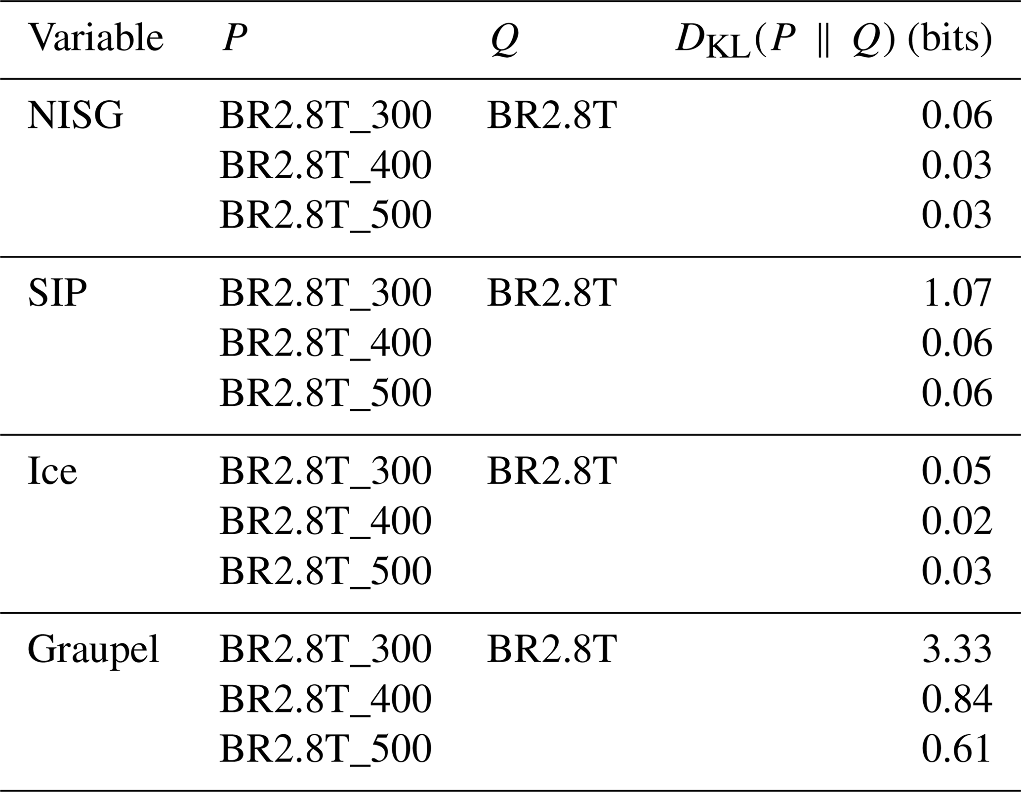
In this section the sensitivity of SIP to the rate of graupel formation, which is dependent on ice or snow crystals being larger than a given size when riming occurs, is analyzed. Figure C1 shows the particle size distribution (PSD) for the sensitivity studies during which the size restrictions are modified, which could slow the conversion process of the ice crystals and snow particles to graupel. The PSD over the cross section at 15:30 UTC showed little difference in the ice crystal number concentrations where we expected higher ice crystal number concentration for BR2.8T and consequently higher snow number concentrations due to enhanced aggregation (Fig. C1a and b). The largest differences from the BR2.8T_300 simulation were in the form of enhanced snow (for diameters $\mathrm{0.14}<{\stackrel{\mathrm{‾}}{D}}_{\mathrm{s}}<\mathrm{0.42}$ mm) and graupel number concentrations (for diameters $\mathrm{1.2}<{\stackrel{\mathrm{‾}}{D}}_{\mathrm{g}}<\mathrm{2.2}$ mm). However, at 15:30 UTC there is no clear signal beyond model variability, showing that the slower conversion rates to graupel affect the simulations (Fig. C1b and c). We compared the probability distributions of the total number of ice hydrometeors (NISG, i.e., ice crystals, snow and graupel), SIP rate, ice crystal and graupel number concentrations of the BR2.8T_500, BR2.8T_400 and BR2.8T_300 simulations, respectively, to that of the reference simulation, BR2.8T, between 14:15 and 15:45 UTC (Fig. 8b). We chose this time period as the largest graupel concentrations were present. The Kullback–Leibler divergence (D_KL(P ∥ Q)), which measures how one probability distribution P is different from a second probability distribution Q, shows little information loss between variables in Table C1, except for graupel. A value of 0 bits means that the probability distributions are the same (e.g., no information loss). The largest D_KL(BR2.8T_300 ∥ BR2.8T) was 3.33 bits for the graupel distribution and was reflected in larger differences in the SIP rate of 1.07 bits and ice number concentration of 0.05 bits (Table C1 and Fig. C1c). If the SIP rate was sensitive to the conversion rate, it is expected that the information loss would be the greatest between BR2.8T_500 and BR2.8T and not between BR2.8T_300 and BR2.8T (e.g., D_KL(BR2.8T_500 ∥ BR2.8T) >D_KL(BR2.8T_400 ∥ BR2.8T) >D_KL(BR2.8T_300 ∥ BR2.8T)). This result leads us to conclude that the different conversion rate size thresholds from ice crystals and snow to graupel, used in the paper in conjunction with the collisional-breakup parameterization, were not significant for SIP.

Table C1 The Kullback–Leibler divergence, D_KL(P ∥ Q), between two probability distributions P and Q from 14:14 to 15:45 UTC. P (BR2.8T_300, BR2.8T_400 and BR2.8T_500) is the measured probability distribution against the reference probability distribution Q (BR2.8T). Each distribution consist of ∼10 800 grid points separated into 24 bins over the cross section in Fig. 1.